A Metapopulation Model of Chagas Disease in Colombia with HumanMobility

Jasmine Jackson1, Diana Carolina Erazo2, Luisa Rodriguez2, Juliana Noguera2, Liliana Piñeros21Arizona State University, Tempe, AZ

2Universidad de Los Andes, Bogotá, Colombia

July 20, 2015

1 Introduction

Chagas disease, also known as American trypanosomiasis, is a zoonose and a tropical parasitic infection that orig-inated in the Americas and is caused by the flagellate protozoan Trypanosoma cruzi [11]. Discovered in 1909,Chagas disease was progressively shown to be widespread throughout Latin America, affecting millions of ruralregions with a high impact on morbidity and mortality. In the last few years, the disease has become an emergingimport and has spread to countries in North America, Asia, and Europe due to the migration from Latin Amer-icas [10]. There are approximately 8 to 10 million people in Latin America, who suffer from Chagas disease andanother 28 million who are at risk of contracting it [18].

The most domestic specie is Triatoma infestans and it is the principal vector of the Southern cone. In northernSouth America geographical insect distribution changes, the Rhodnius prolixus, a blood-sucking triatomine withdomiciliary anthropophilic habits, is the main vector of Chagas disease. The current paradigm of Trypanosomacruzi (T. cruzi) transmission in Colombia includes a sylvatic and domiciliary cycle co-existing with domestic andsylvatic populations of reservoirs. The eco-epidemiological factors shape the transmission dynamics of T. cruzi,creating diverse scenarios of disease transmission [22]. Infection cycle occurs when an infected triatomine insectvector (or "kissing" bug) takes a blood meal and releases trypomastigotes in its feces near the site of the bitewound. Trypomastigotes enter the host through the wound or through intact mucosal membranes, such as theconjunctiva.

In Colombia, the prevalence of Chagas disease has been estimated as 1,300,000 habitants infected and 3,500,000habitants at risk of infection depending on the geographical distribution of the vector [13]; hence, establishingendemic areas throughout the country. The principal endemic areas are: Caribbean coastal region, Orinoquiaregion, and Andes mountain region. The risk of infection varies in each endemic area in the country (Figure1). There are several reasons for this change. The principal reason is the difference among the environmentalcharacteristics in each region that affect the life cycle of the vector. Furthermore, allowing for the creation ofvariable interactions between vector and host in these specific areas increasing or decreasing the risk of infection.There has been a reasonable number of cases confirmed in Bogotá where there are no parasites. This is an alarmingfinding. We would like to mathematically ascertain if human mobility is contributing to the dispersal and incidenceof Chagas disease.

1

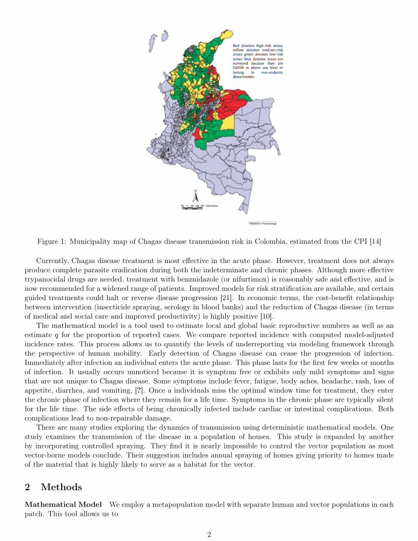
Figure 1: Municipality map of Chagas disease transmission risk in Colombia, estimated from the CPI [14]

Currently, Chagas disease treatment is most effective in the acute phase. However, treatment does not alwaysproduce complete parasite eradication during both the indeterminate and chronic phases. Although more effectivetrypanocidal drugs are needed, treatment with benznidazole (or nifurtimox) is reasonably safe and effective, and isnow recommended for a widened range of patients. Improved models for risk stratification are available, and certainguided treatments could halt or reverse disease progression [21]. In economic terms, the cost-benefit relationshipbetween intervention (insecticide spraying, serology in blood banks) and the reduction of Chagas disease (in termsof medical and social care and improved productivity) is highly positive [10].

The mathematical model is a tool used to estimate local and global basic reproductive numbers as well as anestimate q for the proportion of reported cases. We compare reported incidence with computed model-adjustedincidence rates. This process allows us to quantify the levels of underreporting via modeling framework throughthe perspective of human mobility. Early detection of Chagas disease can cease the progression of infection.Immediately after infection an individual enters the acute phase. This phase lasts for the first few weeks or monthsof infection. It usually occurs unnoticed because it is symptom free or exhibits only mild symptoms and signsthat are not unique to Chagas disease. Some symptoms include fever, fatigue, body aches, headache, rash, loss ofappetite, diarrhea, and vomiting, [?]. Once a individuals miss the optimal window time for treatment, they enterthe chronic phase of infection where they remain for a life time. Symptoms in the chronic phase are typically silentfor the life time. The side effects of being chronically infected include cardiac or intestinal complications. Bothcomplications lead to non-repairable damage.

There are many studies exploring the dynamics of transmission using deterministic mathematical models. Onestudy examines the transmission of the disease in a population of houses. This study is expanded by anotherby incorporating controlled spraying. They find it is nearly impossible to control the vector population as mostvector-borne models conclude. Their suggestion includes annual spraying of homes giving priority to homes madeof the material that is highly likely to serve as a habitat for the vector.

2 Methods

Mathematical Model We employ a metapopulation model with separate human and vector populations in eachpatch. This tool allows us to

2

• study within and across patch transmission dynamics,

• assess potential heterogeneity contributions on epidemics, and

• synchrony between populations (leader-follower regions), [23].

The model is inspired by the two-patch model incorporating resident time by Lee & Castillo-Chavez, [17]. Inthe analysis of Lee & Castillo-Chavez, they focused on the influence of human mobility between two patches onthe temporal sequence of disease spread between patches, thus, showing the influence of movement and the basicreproduction number R0 on the relative timing of epidemic peaks.For our model, each patch is derived on the basis of ecological and epidemiological reasoning. Furthermore, eachpatch has a principle vector with an unique transmission rate. We will define a deterministic model for the diseasein each patch.

1

23

4

5

67

89

10

Model patches

illustration of model connections

Figure 2: Patches with heterogeneous environments that could affect the transmission Chagas disease.

Natural regionsAmazon forest Orinoquia lowlands Pacific coast Caribean lowlands Andean region Sierra Nevada

Figure 3: Principle vectors for each region in Colombia REFERENCE?

The rate of change for susceptible, acutely infectious, chronically infectious, and treated humans are considered.Also, the susceptible and infectious vectors’ rate of change are included. This is the first time, to our knowledge,the infectious class for humans have been subdivided while modeling Chagas disease. Pathologically, the infectionstage is divided into three phases: acute, latent, and chronic. We consider the acute and latent phase as one statebecause the latent stage is completely asymptomatic and coined as indeterminate. After several months, yearsor decades, about 30% of infected humans enter into a chronic stage consisting of severe cardiomyopathy and/orgastrointestinal dysfunctions [9]. During the acute phase, there is evidence of high levels of parasitemia followed

3

by a significant decrease during the chronic stage. Experimental rat data suggests that after the initial spikein parasitemia, the host does not experience the same spiked level of parasitemia again and a remarkable lesseramount of blood circulating parasites were recorded during this period of observation. Hence, hinting at somesort of immunity where the host immune system is able to control the parasite proliferation through mediatingmechanisms as the humoral response [3]. The parasitemia levels alter the effective transmission from an infectioushuman to susceptible vector. We explore this phenomena closely.

State Variable Description

Sh Population of susceptible humans

Ih Population of acutely infected humans

Ch Population of chronically infected humans

Th Population of humans in treatment

Sv Population of susceptible vectors

Iv Population of infected vectors

Table 1: Subpopulations of the model and descriptions

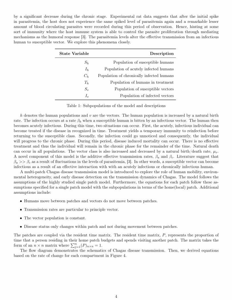
h denotes the human populations and v are the vectors. The human population is increased by a natural birthrate. The infection occurs at a rate βh when a susceptible human is bitten by an infectious vector. The human thenbecomes acutely infectious. During this time, two situations can occur. First, the acutely, infectious individual canbecome treated if the disease in recognized in time. Treatment yields a temporary immunity to reinfection beforereturning to the susceptible class. Secondly, the infection could go unnoticed and consequently, the individualwill progress to the chronic phase. During this period, disease induced mortality can occur. There is no effectivetreatment and thus the individual will remain in the chronic phase for the remainder of the time. Natural deathcan occur in all populations. The vector class is also increased and decreased by a natural birth/death rate, µv.A novel component of this model is the additive effective transmission rates, βa and βc. Literature suggest thatβa >> βc as a result of fluctuations in the levels of parasitemia, [3]. In other words, a susceptible vector can becomeinfectious as a result of an effective interaction with with an acutely infectious or chronically infectious human.

A multi-patch Chagas disease transmission model is introduced to explore the role of human mobility, environ-mental heterogeneity, and early disease detection on the transmission dynamics of Chagas. The model follows theassumptions of the highly studied single patch model. Furthermore, the equations for each patch follow these as-sumptions specified for a single patch model with the subpopulations in terms of the home(local) patch. Additionalassumptions include:

• Humans move between patches and vectors do not move between patches.

• Transmission rates are particular to principle vector.

• The vector population is constant.

• Disease status only changes within patch and not during movement between patches.

The patches are coupled via the resident time matrix. The resident time matrix, P , represents the proportion oftime that a person residing in their home patch budgets and spends visiting another patch. The matrix takes theform of an n× n matrix where

∑nj=1(P )n×n = 1.

The flow diagram demonstrates the schematics of Chagas disease transmission. Then, we derived equationsbased on the rate of change for each compartment in Figure 4.

4

Figure 4: Schematics of Chagas disease transmission.

The multi-patch model dynamics are captured by the following patch-specific system of nonlinear ordinarydifferential equations:Humans

S′hi = µhNhi − Shin∑j=1

βhjpijIvj + ηThi − µhShi (1)

I ′hi = Shi

n∑j=1

βhjpijIvj − qγIhi − (1− q)γIhi − µhIhi (2)

C ′hi = qiγIhi − (µh + δc)Chi (3)T ′hi = (1− qi)γIhi − µhThi − ηThi (4)

Vectors

S′vi = µvNvi − Svi

βa n∑j=1

pjiIhj + βc

n∑j=1

pjiChj

− µvSvi (5)

I ′vi = Svi

βa n∑j=1

pjiIhj + βc

n∑j=1

pjiChj

− µvIvi (6)

for i = 1, 2. Chagas disease has a very long infectious period that ranges from 10 to 30 years in the chronic stage.As a result, we believe it is inappropriate to assume a constant human population. On the other hand, assuminga constant vector population seems reasonable. The model should consist of both natural and disease inducedmortality.

Human Mobility We are assuming that human travel contributes to the spread of the disease, as the vectorsonly travel a very limited distance. The idea of modeling human movement using the resident time matrix approachis inspired by the work of Lee & Castillo-Chavez [17]. We assume that individuals do not move permanently fromtheir patch of residence to another patch, but may visit other patches. The rate at which individuals becomeinfected then depends upon the fraction of their time that they spend in each patch together with the transmissionrates in those patches. This approach is the Lagrangian in that it labels and, in some sense, tracks individualhumans or vectors [7].

5

3 Quantities of Interest

4 Disease Free Equilibrium and Basic Reproduction Number

4.1 Single Patch Analysis

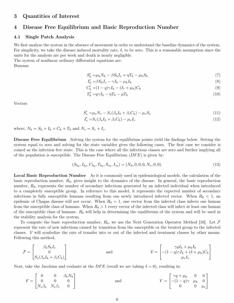
We first analyze the system in the absence of movement in order to understand the baseline dynamics of the system.For simplicity, we take the disease induced mortality rate, δ, to be zero. This is a reasonable assumption since theunits for the analysis are per week and death is nearly negligible.The system of nonlinear ordinary differential equations are:Humans

S′h =µhNh − βShIv + ηTh − µhSh (7)I ′h =βShIv − γIh − µhIh (8)C ′h =(1− q)γIh − (δc + µh)Ch (9)T ′h =qγIh − ηTh − µTh (10)

Vectors

S′v =µvNv − Sv(βaIh + βcCh)− µvSv (11)I ′v =Sv(βaIh + βcCh)− µvIv (12)

where, Nh = Sh + Ih + Ch + Th and Nv = Sv + Iv.

Disease Free Equilibrium Solving the system for the equilibrium points yield the findings below. Setting thesystem equal to zero and solving for the state variables gives the following cases. The first case we consider iscoined as the infection free state. This is the case where all the infectious classes are zero and further implying allof the population is susceptible. The Disease Free Equilibrium (DFE) is given by:

(Sh0 , Ih0 , Ch0 , Th0 , Sv0 , Iv0) = (Nh, 0, 0, 0, Nv, 0, 0). (13)

Local Basic Reproduction Number As it is commonly used in epidemiological models, the calculation of thebasic reproduction number, R0, gives insight to the dynamics of the disease. In general, the basic reproductionnumber, R0, represents the number of secondary infections generated by an infected individual when introducedto a completely susceptible group. In reference to this model, it represents the expected number of secondaryinfections in fully susceptible humans resulting from one newly introduced infected vector. When R0 < 1, anepidemic of Chagas disease will not occur. When R0 = 1, one vector from the infected class infects one humanfrom the susceptible class of humans. When R0 > 1 every vector of the infected class will infect at least one humanof the susceptible class of humans. R0 will help in determining the equilibrium of the system and will be used inthe stability analysis for the system.

To compute the basic reproduction number, R0, we use the Next Generation Operator Method [16]. Let Frepresent the rate of new infections caused by transition from the susceptible or the treated group to the infectedclasses. V will symbolize the rate of transfer into or out of the infected and treatment classes by other means.Following this method,

F =

βhShIv0

Sv(βaIh + βcCh)

and V =

γqIh + µhIh−(1− q)γIh + (δ + µh)Ch

µvIv

Next, take the Jacobian and evaluate at the DFE (recall we are taking δ = 0), resulting in:

F =

0 0 βhNh

0 0 0Nvβa Nvβc 0

and V =

γq + µh 0 0−(1− q)γ µh 0

0 0 µv

6

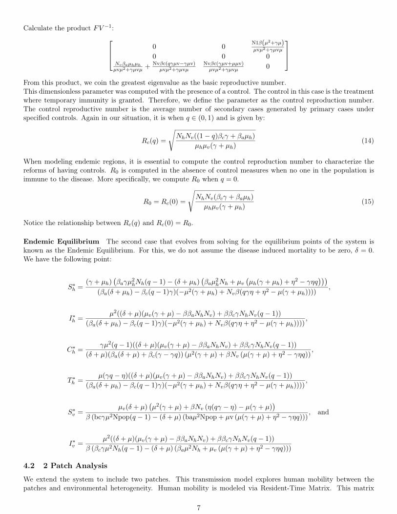
Calculate the product FV −1: 0 0N1β(µ2+γµ)µvµ2+γµvµ

0 0 0Nvβaµhµhµvµ2+γµvµ + Nvβc(qγµv−γµv)

µvµ2+γµvµNvβc(γµv+µµv)µvµ2+γµvµ 0

From this product, we coin the greatest eigenvalue as the basic reproductive number.This dimensionless parameter was computed with the presence of a control. The control in this case is the treatmentwhere temporary immunity is granted. Therefore, we define the parameter as the control reproduction number.The control reproductive number is the average number of secondary cases generated by primary cases underspecified controls. Again in our situation, it is when q ∈ (0, 1) and is given by:

Rc(q) =

√NhNv((1− q)βcγ + βaµh)

µhµv(γ + µh)(14)

When modeling endemic regions, it is essential to compute the control reproduction number to characterize thereforms of having controls. R0 is computed in the absence of control measures when no one in the population isimmune to the disease. More specifically, we compute R0 when q = 0.

R0 = Rc(0) =

√NhNv(βcγ + βaµh)

µhµv(γ + µh)(15)

Notice the relationship between Rc(q) and Rc(0) = R0.

Endemic Equilibrium The second case that evolves from solving for the equilibrium points of the system isknown as the Endemic Equilibrium. For this, we do not assume the disease induced mortality to be zero, δ = 0.We have the following point:

S∗h =(γ + µh)

(βaγµ

2hNh(q − 1)− (δ + µh)

(βaµ

2hNh + µv

(µh(γ + µh) + η2 − γηq

)))(βa(δ + µh)− βc(q − 1)γ)(−µ2(γ + µh) +Nvβ(qγη + η2 − µ(γ + µh))))

,

I∗h =µ2((δ + µ)(µv(γ + µ)− ββaNhNv) + ββcγNhNv(q − 1))

(βa(δ + µh)− βc(q − 1)γ)(−µ2(γ + µh) +Nvβ(qγη + η2 − µ(γ + µh)))),

C∗h =γµ2(q − 1)((δ + µ)(µv(γ + µ)− ββaNhNv) + ββcγNhNv(q − 1))

(δ + µ)(βa(δ + µ) + βc(γ − γq)) (µ2(γ + µ) + βNv (µ(γ + µ) + η2 − γηq)),

T ∗h =µ(γq − η)((δ + µ)(µv(γ + µ)− ββaNhNv) + ββcγNhNv(q − 1))

(βa(δ + µh)− βc(q − 1)γ)(−µ2(γ + µh) +Nvβ(qγη + η2 − µ(γ + µh)))),

S∗v =µv(δ + µ)

(µ2(γ + µ) + βNv (η(qγ − η)− µ(γ + µ)

)β (bcγµ2Npop(q − 1)− (δ + µ) (baµ2Npop + µv (µ(γ + µ) + η2 − γηq)))

, and

I∗v =µ2((δ + µ)(µv(γ + µ)− ββaNhNv) + ββcγNhNv(q − 1))

β (βcγµ2Nh(q − 1)− (δ + µ) (βaµ2Nh + µv (µ(γ + µ) + η2 − γηq)))

4.2 2 Patch Analysis

We extend the system to include two patches. This transmission model explores human mobility between thepatches and environmental heterogeneity. Human mobility is modeled via Resident-Time Matrix. This matrix

7

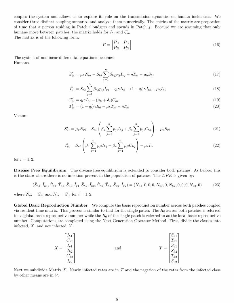
couples the system and allows us to explore its role on the transmission dynamics on human incidences. Weconsider three distinct coupling scenarios and analyze them numerically. The entries of the matrix are proportionof time that a person residing in Patch i budgets and spends in Patch j. Because we are assuming that onlyhumans move between patches, the matrix holds for Ihi and Chi.The matrix is of the following form:

P =

[P11 P12

P21 P22

](16)

The system of nonlinear differential equations becomes:Humans

S′hi = µhNhi − Shin∑j=1

βhjpijIvj + ηThi − µhShi (17)

I ′hi = Shi

n∑j=1

βhjpijIvj − qiγIhi − (1− qi)γIhi − µhIhi (18)

C ′hi = qiγIhi − (µh + δc)Chi (19)T ′hi = (1− qi)γIhi − µhThi − ηThi (20)

Vectors

S′vi = µvNvi − Svi

βa n∑j=1

pjiIhj + βc

n∑j=1

pjiChj

− µvSvi (21)

I ′vi = Svi

βa n∑j=1

pjiIhj + βc

n∑j=1

pjiChj

− µvIvi (22)

for i = 1, 2.

Disease Free Equilibrium The disease free equilibrium is extended to consider both patches. As before, thisis the state where there is no infection present in the population of patches. The DFE is given by:

(Sh1, Ih1, Ch1, Th1, Sv1, Iv1, Sh2, Ih2, Ch2, Th2, Sv2, Iv2) = (Nh1, 0, 0, 0, Nv1, 0, Nh2, 0, 0, 0, Nv2, 0) (23)

where Nhi = Shi and Nvi = Svi for i = 1, 2.

Global Basic Reproduction Number We compute the basic reproduction number across both patches coupledvia resident time matrix. This process is similar to that for the single patch. The R0 across both patches is referredto as global basic reproductive number while the R0 of the single patch is referred to as the local basic reproductivenumber. Computations are completed using the Next Generation Operator Method. First, divide the classes intoinfected, X, and not infected, Y .

X =

Ih1Ch1Iv1Ih2Ch2Iv2

and Y =

Sh1Th1Sv1Sh2Th2Sv2

Next we subdivide Matrix X. Newly infected rates are in F and the negation of the rates from the infected classby other means are in V.

8

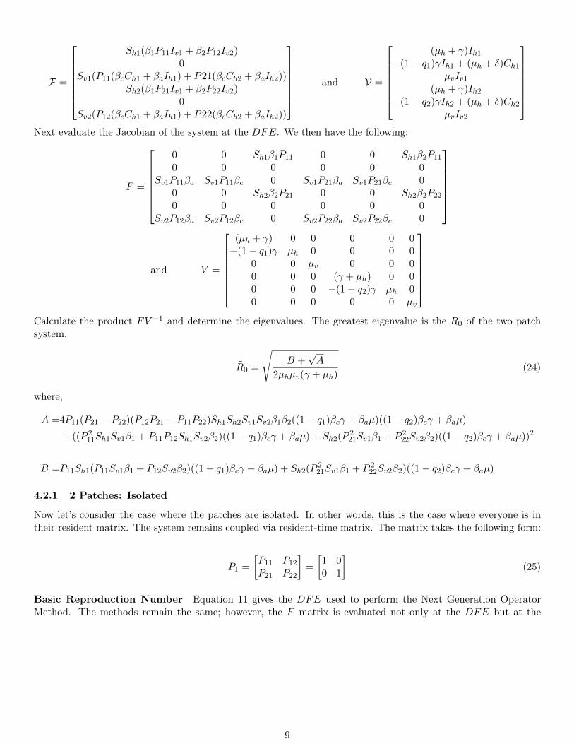
F =

Sh1(β1P11Iv1 + β2P12Iv2)0

Sv1(P11(βcCh1 + βaIh1) + P21(βcCh2 + βaIh2))Sh2(β1P21Iv1 + β2P22Iv2)

0Sv2(P12(βcCh1 + βaIh1) + P22(βcCh2 + βaIh2))

and V =

(µh + γ)Ih1−(1− q1)γIh1 + (µh + δ)Ch1

µvIv1(µh + γ)Ih2

−(1− q2)γIh2 + (µh + δ)Ch2µvIv2

Next evaluate the Jacobian of the system at the DFE. We then have the following:

F =

0 0 Sh1β1P11 0 0 Sh1β2P11

0 0 0 0 0 0Sv1P11βa Sv1P11βc 0 Sv1P21βa Sv1P21βc 0

0 0 Sh2β2P21 0 0 Sh2β2P22

0 0 0 0 0 0Sv2P12βa Sv2P12βc 0 Sv2P22βa Sv2P22βc 0

and V =

(µh + γ) 0 0 0 0 0−(1− q1)γ µh 0 0 0 0

0 0 µv 0 0 00 0 0 (γ + µh) 0 00 0 0 −(1− q2)γ µh 00 0 0 0 0 µv

Calculate the product FV −1 and determine the eigenvalues. The greatest eigenvalue is the R0 of the two patchsystem.

R0 =

√B +

√A

2µhµv(γ + µh)(24)

where,

A =4P11(P21 − P22)(P12P21 − P11P22)Sh1Sh2Sv1Sv2β1β2((1− q1)βcγ + βaµ)((1− q2)βcγ + βaµ)

+ ((P 211Sh1Sv1β1 + P11P12Sh1Sv2β2)((1− q1)βcγ + βaµ) + Sh2(P

221Sv1β1 + P 2

22Sv2β2)((1− q2)βcγ + βaµ))2

B =P11Sh1(P11Sv1β1 + P12Sv2β2)((1− q1)βcγ + βaµ) + Sh2(P221Sv1β1 + P 2

22Sv2β2)((1− q2)βcγ + βaµ)

4.2.1 2 Patches: Isolated

Now let’s consider the case where the patches are isolated. In other words, this is the case where everyone is intheir resident matrix. The system remains coupled via resident-time matrix. The matrix takes the following form:

P1 =

[P11 P12

P21 P22

]=

[1 00 1

](25)

Basic Reproduction Number Equation 11 gives the DFE used to perform the Next Generation OperatorMethod. The methods remain the same; however, the F matrix is evaluated not only at the DFE but at the

9

’identity’ ,P1, as well.

F(P11=1,P12=0,P21=0,P22=1) =

0 0 Sh1β1P11 0 0 Sh1β2P11

0 0 0 0 0 0Sv1P11βa Sv1P11βc 0 Sv1P21βa Sv1P21βc 0

0 0 Sh2β2P21 0 0 Sh2β2P22

0 0 0 0 0 0Sv2P12βa Sv2P12βc 0 Sv2P22βa Sv2P22βc 0

V =

(µh + γ) 0 0 0 0 0−(1− q1)γ µh 0 0 0 0

0 0 µv 0 0 00 0 0 (γ + µh) 0 00 0 0 −(1− q1)γ µh 00 0 0 0 0 µv

After solving the product FV −1 and the eigenvalues. We find that the basic reproductive number for the twopatch, isolated case is below:

R0 = max

{β2Sh2Sv2(βaµh + βcγ(1− q2))

µhµv(γ + µh),β1Sh1Sv1(βaµh + βcγ(1− q1))

µhµv(γ + µh)

}(26)

5 Results

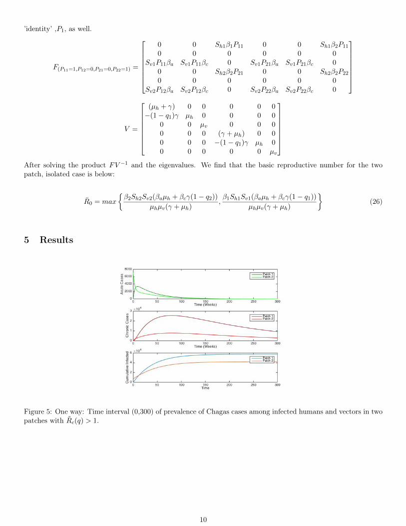
Figure 5: One way: Time interval (0,300) of prevalence of Chagas cases among infected humans and vectors in twopatches with Rc(q) > 1.

10

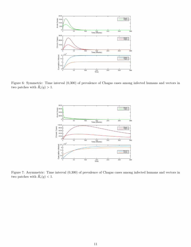
Figure 6: Symmetric: Time interval (0,300) of prevalence of Chagas cases among infected humans and vectors intwo patches with Rc(q) > 1.

Figure 7: Asymmetric: Time interval (0,300) of prevalence of Chagas cases among infected humans and vectors intwo patches with Rc(q) < 1.

11

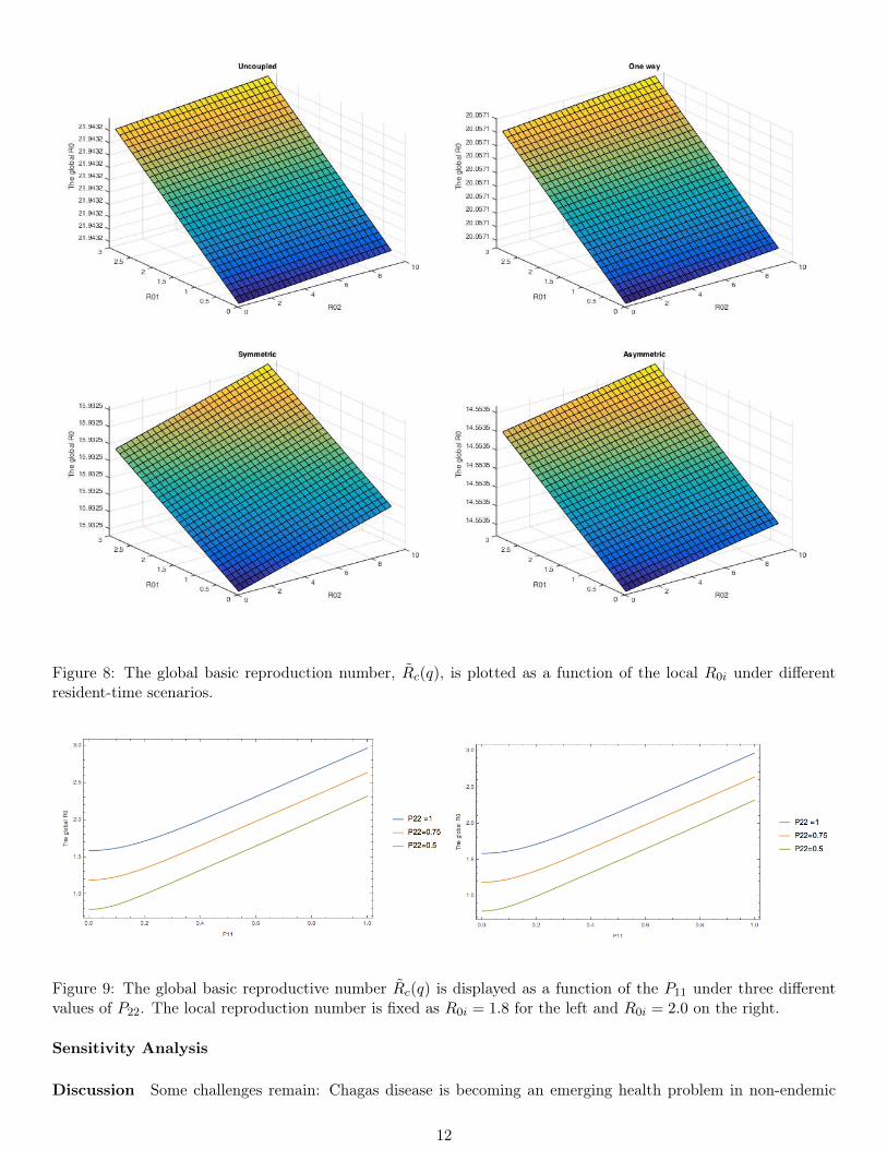
Figure 8: The global basic reproduction number, Rc(q), is plotted as a function of the local R0i under differentresident-time scenarios.

Figure 9: The global basic reproductive number Rc(q) is displayed as a function of the P11 under three differentvalues of P22. The local reproduction number is fixed as R0i = 1.8 for the left and R0i = 2.0 on the right.

Sensitivity Analysis

Discussion Some challenges remain: Chagas disease is becoming an emerging health problem in non-endemic

12

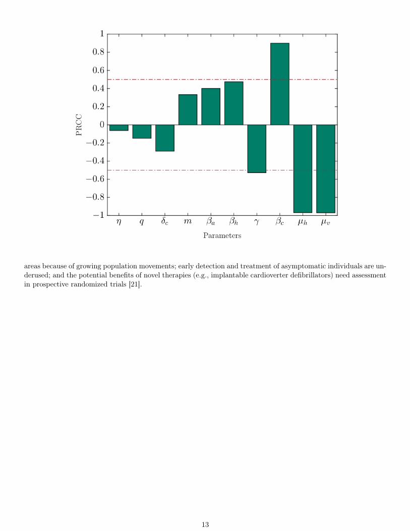
areas because of growing population movements; early detection and treatment of asymptomatic individuals are un-derused; and the potential benefits of novel therapies (e.g., implantable cardioverter defibrillators) need assessmentin prospective randomized trials [21].

13

6 Acknowledgements

We would like to thank the Universidad de los Andes in Bogotà and the Simon A. Levin Mathematical, Compu-tational and Modeling Sciences Center at Arizona State University for sponsoring the first International ResearchExperience (IRES) Program. We would also like to Juan Manuel Cordovez and Carlos Castillo-Chavez for theirinvaluable support and insights into this paper.

14

References

[1] Miguel A Acevedo, Olivia Prosper, Kenneth Lopiano, Nick Ruktanonchai, T Trevor Caughlin, Maia Martcheva,Craig W Osenberg, and David L Smith. Spatial heterogeneity, host movement and vector-borne disease.

[2] Elaine T Alexander, Savanah D McMahon, Nicholas Roberts, Emilio Sutti, Daniel Burkow, Miles Manning,Kamuela E Yong, and Sergei Suslov. The effects of regional vaccination heterogeneity on measles outbreakswith france as a case study. arXiv preprint arXiv:1408.0695, 2014.

[3] Néstor Añez, María Luisa Martens, Maximiliano Romero, and Gladys Crisante. Trypanosoma cruzi primaryinfection prevents severe re-infection in mice primoinfección por trypanosoma cruzi previene re-infeccionesseveras en ratones. 2011.

[4] Crystal Bennett. Dynamics of triatomine infestation in a population of houses. 2013.

[5] Samuel Bowong, Yves Dumont, and Jean Jules Tewa. A patchy model for chikungunya-like diseases. Biomath,2(1):Article–ID, 2013.

[6] Marianela Castillo-Riquelme, Felipe Guhl, Brenda Turriago, Nestor Pinto, Fernando Rosas, Mónica FlórezMartínez, Julia Fox-Rushby, Clive Davies, and Diarmid Campbell-Lendrum. The costs of preventing andtreating chagas disease in colombia. PLoS Negl Trop Dis, 2(11):e336, 2008.

[7] C Cosner, JC Beier, RS Cantrell, D Impoinvil, L Kapitanski, MD Potts, A Troyo, and S Ruan. The effects ofhuman movement on the persistence of vector-borne diseases. Journal of theoretical biology, 258(4):550–560,2009.

[8] Britnee Crawford and Christopher Kribs-Zaleta. A metapopulation model for sylvatic t. cruzi transmissionwith vector migration. Mathematical biosciences and engineering: MBE, 11(3):471–509, 2014.

[9] Hugo Devillers, Jean Raymond Lobry, and Frédéric Menu. An agent-based model for predicting the prevalenceof trypanosoma cruzi i and ii in their host and vector populations. Journal of theoretical biology, 255(3):307–315, 2008.

[10] João Carlos Pinto Dias, Antonio Carlos Silveira, and Christopher John Schofield. The impact of chagas diseasecontrol in latin america: a review. Memórias do Instituto Oswaldo Cruz, 97(5):603–612, 2002.

[11] Nelson Ferreira Fé, Maria das Graças Vale Barbosa, Flávio Augusto Andrade Fé, MV de F Guerra, andWilson Duarte Alecrim. Fauna de culicidae em municípios da zona rural do estado do amazonas, com incidênciade febre amarela. Rev Soc Bras Med Trop, 36:343–348, 2003.

[12] Marcel Munoz Figueroa, Xavier Martınez Rivera, Thomas Seaquist, Britnee Crawford, Anuj Mubayi, KehindeSalau, and Christopher Kribs-Zaleta. Two strain competition: Trypanosoma cruzi. Technical report, Tech.Rep., MTBI-06-07M, Arizona State University, 2009. Available at mtbi. asu. edu.

[13] Felipe Guhl, Germán Aguilera, Néstor Pinto, and Daniela Vergara. Actualización de la distribución geográficay ecoepidemiología de la fauna de triatominos (reduviidae: Triatominae) en colombia. Biomédica, 27:143–162,2007.

[14] Felipe Guhl, Marco Restrepo, Victor Manuel Angulo, Carlos MF Antunes, Diarmid Campbell-Lendrum, andClive R Davies. Lessons from a national survey of chagas disease transmission risk in colombia. TRENDS inParasitology, 21(6):259–262, 2005.

[15] Ilkka Hanski. Metapopulation dynamics. Nature, 396(6706):41–49, 1998.

[16] JAP Heesterbeek. Mathematical epidemiology of infectious diseases: model building, analysis and interpreta-tion, volume 5. John Wiley & Sons, 2000.

[17] Sunmi Lee and Carlos Castillo-Chavez. The role of residence times in two-patch dengue transmission dynamicsand optimal strategies. Journal of theoretical biology, 374:152–164, 2015.

15

[18] Juan Diego Maya, Myriam Orellana, Jorge Ferreira, Ulrike Kemmerling, Rodrigo López-Muñoz, and AntonioMorello. Chagas disease: Present status of pathogenic mechanisms and chemotherapy. Biological research,43(3):323–331, 2010.

[19] Djamila Moulay and Yoann Pigné. A metapopulation model for chikungunya including populations mobilityon a large-scale network. Journal of theoretical biology, 318:129–139, 2013.

[20] Víctor H Peña-García, Andrés M Gómez-Palacio, Omar Triana-Chávez, and Ana M Mejía-Jaramillo. Eco-epidemiology of chagas disease in an endemic area of colombia: Risk factor estimation, trypanosoma cruzicharacterization and identification of blood-meal sources in bugs. The American journal of tropical medicineand hygiene, 91(6):1116–1124, 2014.

[21] Anis Rassi and José Antonio Marin-Neto. Chagas disease. The Lancet, 375(9723):1388–1402, 2010.

[22] Lina María Rendón, Felipe Guhl, Juan Manuel Cordovez, and Diana Erazo. New scenarios of trypanosomacruzi transmission in the orinoco region of colombia. Memórias do Instituto Oswaldo Cruz, (AHEAD):00–00,2015.

[23] Marta Sarzynska, Oyita Udiani, and Na Zhang. A study of gravity-linked metapopulation models for thespatial spread of dengue fever. arXiv preprint arXiv:1308.4589, 2013.

[24] Anna Maria Spagnuolo, Meir Shillor, and Gabrielle A Stryker. A model for chagas disease with controlledspraying. Journal of Biological Dynamics, 5(4):299–317, 2011.

[25] Min Su, Wenlong Li, Zizhen Li, Fengpan Zhang, and Cang Hui. The effect of landscape heterogeneity onhost–parasite dynamics. Ecological research, 24(4):889–896, 2009.

16