a method for testing anisotropy and quantifying its direction in digital images

Computers & Graphics 26 (2002) 771–784

Technical section

A method for testing anisotropy and quantifying its directionin digital images

Andr!es Molina, Francisco R. Feito*

Dpto de Inform !atica, Escuela Polit!ecnica Superior, Universidad de Ja!en. Avda. de Madrid 35, 23071 Ja!en, Spain

Abstract

The identification of appropriate spatial models requires the previous knowledge of the process exploratory

properties such as the degree of homogeneity in local and global effects, and the existence of a directional component

which determines an anisotropic behaviour of the phenomenon. This will allow the assumption of some form of

stationarity that reduces the number of parameters involved in the model so that it becomes manageable. The methods

for exploring stationarity both from global and local levels are varied and well-known. Techniques used for analysing

anisotropy are, on the contrary, limited and they are only devoted to examining ‘‘by eye’’ experimental variograms in

different directions. In this paper, we present a method based on second-order bivariate circular statistics that allows us

to determine the anisotropy existence in digital images and the quantification of the direction in which this appears. A

study about the flow of seawater through the Strait of Gibraltar, based on a remotely sense image, is presented as an

example of the potential use of the proposed method. r 2002 Elsevier Science Ltd. All rights reserved.

Keywords: Statistical model; Model validation and analysis; Circular statistics; Standard and confidence ellipses

1. Introduction and motivation

The specification of a statistical spatial model requires

first of all, the visualization of data in an adequate way,

usually by a map. In order to acquire a greater

knowledge of the phenomenon behaviour, exploratory

techniques will be applied on this map. From the

information obtained, we will try to generate a statistical

model by the specification of one or more probability

functions for each of the random variables involved in

the process. This task can be difficult or even impossible;

so, when a formal specification of the phenomenon is

necessary, the researcher employs artefacts that, not

being real, allow him to design a model that reproduces

the phenomenon in a approximate way. In general, the

behaviour of spatial phenomena is often the result of a

mixture of both first-order and second-order effects.

First-order effects relate to variation in the mean value

of the process in the space (a global or large-scale trend).

Second-order effects result from the spatial correlation

structure, or the spatial dependence in the process, and

they are concerned with the behaviour of stochastic

deviations from this mean (local or small scale effects).

The second-order component is often modelled as a

stationary spatial process. Informally, a spatial process

fZðsÞ; sADg; is stationary or homogeneous if there are no

links between the value of the statistics that describe it

(especially mean and variance) and its location in the

space. Consequently, stationarity implies that mean

EðZðsÞÞ; and variance VARðZðsÞÞ; are constant and

independent of their location in D: Stationarity also

implies that given two points s1 and s2; their covariancevalue CovðZðs1Þ;Zðs2ÞÞ; between values at any two sites,

si; sj ; depends only on the relative locations of these

sites, and not on their absolute location in D: If, in

addition to stationarity, the covariance depends only on

the distance between si and sj ; and not on the direction

in which they are separated, ZðsÞ is isotropic. If, on the

contrary, the covariance presents dependence on the

direction that si and sj form, ZðsÞ is anisotropic [1].

*Corresponding author.

E-mail address: [email protected], [email protected]

(F.R. Feito).

0097-8493/02/$ - see front matter r 2002 Elsevier Science Ltd. All rights reserved.

PII: S 0 0 9 7 - 8 4 9 3 ( 0 2 ) 0 0 1 3 2 - 2

More formally, a spatial process fZðsÞ; sADg satis-

fying

EðZðsÞÞ ¼ m for all sAD;

CovðZðs1Þ;Zðs2ÞÞ ¼ Cðs1 � s2Þ for all s1; s2ADð1Þ

is defined to be second-order stationary. The function

CðhÞ is called a covariogram or a stationary covariance

function. Furthermore, if Cðs1 � s2Þ is function only of

s1 � s2j j; ZðsÞ is isotropic [2]. If the mean, or variance, or

the covariance structure ‘‘drift’’ over D then we say that

the process exhibits non-stationarity or heterogeneity.

Spatial dependence is a special case of homogeneity. It

implies that the data for particular spatial units are

related and similar to data for other nearby spatial units

in a spatially identifiable way [3]. The existence of spatial

dependence is equivalent to the fulfilment of Tobler’s

first law of geography, that establishes that ‘‘everything

is related to everything else but near things are more

related than distant things’’ [4].

The design of spatial models is only possible under the

assumption of stationarity in global and/or local effects.

If no kind of stationarity is assumed, it would be

extremely complex to model the phenomenon due to the

high number of parameters necessary for the mathema-

tical formalization of its behaviour. Besides, it is

necessary to determine if the phenomenon presents

anisotropy, since this fact would invalidate the employ-

ment of models defined for isotropic random functions.

For this reason, the spatial processes modelling requires

not only an analysis of stationarity in global and local

variations, but also a directional study to determine the

existence of an anisotropic component. Many and

varied tools are used for analysing homogeneity [5]:

methods based on tessellation (Delaunay triangulation,

natural neighbourhood interpolation) of the observed

samples to estimate the mean of the parent population,

smoothing methods (spatial moving averages, median

polish) and kernel estimation (kernel density estimation,

adaptive kernel density estimation) to delimit homo-

geneous areas and to identify possible models, k-

functions and covariance functions (covariograms) to

describe, respectively, second-order properties of point

patterns and spatially continuous data, variograms,

statistics of spatial autocorrelation (Moran’s I, Geary’s

C, Getis’ G), autocorrelograms, spatial trend, etc.

Statistical models are widely used in computer graphics,

especially, if not exclusively, in pattern recognition and

computer vision. There is a long history of image

processing algorithms that identify objects in images

with different degrees of uncertainty. These include the

well-known PicHunter System at NEC [6], the eigenface

algorithm for recognizing faces in images at MIT [7,8],

and numerous other probabilistic approaches [9,10].

Statistical models provide important analysis tools

to optimize urban walkthrough algorithms [11],

image processing algorithms for vehicle surveillance

applications [12,13], and compression rates of large

binary images [14].

Anisotropy has been widely applied to obtain an

enhanced image [15–17] or, as a precursor to higher–

level processing, such as shape description [18], edge

detection [19], image segmentation [20], and object

identification and tracking [21]. However, the techniques

used in order to determine the existence of anisotropy in

images are limited, and they just detect directional

effects by inspecting experimental variograms in differ-

ent directions [22]. The examination of these variograms

‘‘by eye’’ only allows a purely informal assessment of the

existence of directedness and an approximate estimation

of the direction in which the anisotropy is revealed.

In this paper, we summarize some of the most

interesting results of our investigation on the application

of circular statistics to handle angles measuring direc-

tions. We present a method that allows, given a digital

image, to determine the existence of anisotropy and to

quantify the direction in which this appears, making

possible the design of anisotropic random functions

from isotropic models [23]. This paper is organized as

follows: Section 2 explains, with an example, the

necessity of establishing a method to test anisotropy

and to measure its direction, describing in Sections 2.1

and 2.2 the tools that will be used for it: standard and

confidence ellipses. Section 3 presents an illustrative

example of directional analysis, studying the global and

local variations previously. Finally, Section 4 completes

the paper.

2. Testing directedness

Fig. 1A is a 17� 17 pixel image, where each pixel has

a light value on the 0–255 grey scale. The lighter

intensities represent values of any random variable ZðsÞ(density of vegetation, concentration of pollen grains in

air, etc.). If 3D plot (Fig. 1B) of the image is displayed,

we can assert that the process behaviour in the north-

west–southeast direction is different from the one

observed in the northeast–southwest one. This fact

highlights two important questions:

* Does an anisotropic behaviour of ZðsÞ really exist, or

on the contrary, is the directional trend observed

caused by random fluctuations?* If anisotropy exits, in which direction is it produced?

The answer to these questions requires the develop-

ment of methods and the use of tools that allow us to

study the spatial variability of the phenomenon, to

establish the existence of anisotropy in a pattern and to

calculate the direction in which this appears. For this,

we will use a parametric procedure based on the

calculation of standard and confidence ellipses.

A. Molina, F.R. Feito / Computers & Graphics 26 (2002) 771–784772

Let Zn;n the matrix that keeps the values of a random

variable ZðsÞ obtained from an image:

Zl;l ¼

z1;l y zl;l

^ ^

z1;1 ? zl;1

264

375: ð2Þ

From Zl;l ; we draw N ¼ fz1; z2;y; zmg; a random

sample of m elements. The vector zizj�! represents a

variation of ZðsÞ with intensity zj � zi

�� in the direction

g; being

g ¼

artanzjy � ziy

zjx � zix

; if zj � zi

� �g0;

Null; if zj � zi

� �¼ 0;

arctanzjy � ziy

zjx � zix

þ p; if zj � zi

� �!0;

8>>>>><>>>>>:

ð3Þ

where ðzix; ziyÞ and ðzjx; zjyÞ are the spatial co-ordinates

of intensities zi and zj ; respectively.

Taking the vectors zizj�!½i ¼ 1;y; ðl � 1Þ; j ¼

ði þ 1Þ;y; l�; we obtain the set

G ¼ gi; i ¼ 1;y; n; n ¼m

2

!( );

that contains the orientations in the plane of vectors

above.

It is evident that, from observations made for a

concrete sample, we cannot draw a conclusion about the

behaviour of values in the image for other samples no

matter how much data is available and how sophisti-

cated the analysis is. For this reason, the statistical

analysis must be performed in two steps, called first and

second-order analysis or first and second stage of

analysis [24]:

* For each sample we reduce the angles gi by

calculating appropriate statistics.* We combine the statistics of the above step and test

their significance. Only then can we make statistical

inference about the directional behaviour of the

population to which the group belongs.

The most suitable measure for our purposes is the

mean vector %m: Given a sample G ¼ fgi; i ¼ 1;y; ng;its mean vector %m (of length r and mean angle %F) is

calculated as follows [25]:

%x ¼1

n

Xn

i

bi cos gi ; %y ¼1

n

Xn

i

bi sin gi ð4Þ

r ¼ffiffiffiffiffiffiffiffiffiffiffiffiffiffiffi%x2 þ %y2

p; %F ¼

arctan%y

%x; if %x > 0;

180þ arctan%y

%x; if %xo0;

8><>: ð5Þ

where

bi ¼0; If gi is Null;

1; If gi is not Null:

(ð6Þ

For each sample G1;y; Gd we determine by first-

order analysis a mean vector of length r and mean angle%F; obtaining the pairs fðri; %FiÞ; i ¼ 1;y; dg: These pairsare supposed to be mutually independent and calculated

from samples with the same number of observations.

Table 2 shows the mean vectors f %mi; i ¼ 1;y; 6gcalculated from the samples N1;y; N6 (Table 1) drawn

from Z17;17 (Fig. 1B).

The vector %m is described by an angle %F and a module

r; in other words, both the angles and the amplitude of

its module have to be considered. Under this condition,

the pairs ðr1; %F1Þ; ðr2; %F2Þ;y; ðrd ; %Fd Þ become a bivariate

and second-order sample, and their treatment is

considered a second-order analysis.

Fig. 1. (A) 17� 17 pixel image, where each pixel has a light

value on the 0–255 grey scale. (B) 3D plot of the image.

A. Molina, F.R. Feito / Computers & Graphics 26 (2002) 771–784 773

2.1. Standard ellipse

Among the tools used for second-order analysis we

can find the standard ellipse. It is exclusively used for

descriptive purposes. The tips of the vectors of a second-

order sample form a scatter diagram of data with

standard deviations in the X and Y directions and a

certain trend upward or downward. The standard ellipse

describes this behaviour in a condensed way: assuming

normality, roughly 40% of data points fall inside the

ellipse and 60% of them outside. The parent population

does not need to be normal, although it is desirable that

it does not deviate from normality too much.

Let ðx1; y1Þ; ðx2; y2Þ;y; ðxd ; yd Þ be a random sample

from a bivariate population. In general, x and y depend

on each other. However, we assume that different pairs

ðxi; yiÞ and ðxk; ykÞ are independent of each other. We

define the standard ellipse in the following way:

* Its centre is at ð %x; %yÞ:* We construct a rectangle with centre at ð %x; %yÞ and

sides parallel to the X and Y axes. The sides are of

length 2s1 and 2s2; respectively.* Standard ellipse is embedded in the rectangle above,

the points of tangency being %x þ rs1; %x � rs1; %x þ s1;%x � s1; %y þ rs2; %y � rs2; %y þ s2; %y � s2:

When drawing the standard ellipse, two means, two

standard deviations and a correlation coefficient are

required:

s21 ¼1

d � 1

Xd

i¼1

ðxi � %xÞ2; s22 ¼1

d � 1

Xd

i¼1

ðyi � %yÞ2; ð7Þ

Covðx; yÞ ¼1

d � 1

Xd

i¼1

ðxi � %xÞðyi � %yÞ;

r ¼ Corrðx; yÞ ¼Covðx; yÞ

s1s2: ð8Þ

The equation of the standard ellipse is

s22ðx � %xÞ2 � 2rs1s2ðx � %xÞðy � %yÞ þ s21ðy � %yÞ2

¼ ð1� r2Þs21s22: ð9Þ

The implicit equation of an ellipse with centre at ð %x; %yÞ is

Aðx � %xÞ2 þ 2Bððx � %xÞðy � %yÞÞ þ Cðx � %xÞ2 ¼ D: ð10Þ

For a standard ellipse, the coefficients are given by

A ¼ s22; B ¼ �rs1s2; C ¼ s21; D ¼ ð1� r2Þs21s22:

ð11Þ

The semi-axes a and b (aob) are

a ¼2D

A þ C � R

1=2; b ¼

2D

A þ C þ R

1=2; ð12Þ

where

R ¼ ½ðA � CÞ2 þ 4B2�1=2: ð13Þ

The sample shows the maximum variability in a

direction of angle y: This is the angle by which the major

axis is inclined versus the X axis (�901oyo901).

y ¼ arctan2B

A � C � R

: ð14Þ

The values of the parameters described, calculated

from Table 2 are the ones shown in Table 3. Fig. 2 shows

the representation of the ellipse.

As we have commented in this section, standard

ellipse is exclusively used for descriptive purposes.

Nevertheless, we can estimate from it, if the assumption

of normality in the parent population is reasonable. If

the mean angles are uniformly spaced around the co-

ordinates origin, we can consider that the population

from which the sample is drawn does not differ from

randomness or one-sideness, avoiding normality. When

this occurs, the confidence ellipse described in the next

subsection is not applicable.

Table 1

Samples N1;y; N6 drawn from Z17;17 in Fig. 1B

z1 z2 z3 z4 z5 z6 z7 z8

N1 (9, 5) (17, 13) (1, 11) (17, 6) (9, 12) (9, 17) (3, 6) (11, 1)

N2 (5, 6) (16, 11) (11, 9) (13, 5) (4, 9) (9, 7) (13, 3) (9, 13)

N3 (13, 15) (4, 5) (4, 13) (9, 2) (4, 4) (8, 9) (12, 16) (17, 7)

N4 (9, 10) (8, 14) (13, 6) (17, 12) (11, 15) (13, 9) (15, 1) (7, 10)

N5 (16, 17) (8, 12) (2, 8) (3, 16) (6, 10) (12, 6) (14, 12) (1, 15)

N6 (7, 7) (5, 4) (9, 16) (14, 3) (3, 10) (17, 8) (2, 17) (14, 17)

Table 2

Mean vectors %mi ; i ¼ 1;y; 6 calculated from the samples

N1; :::; N6 (Table 1), by applying Eqs. (4–6)

i 1 2 3 4 5 6

ri 0.53 0.60 0.49 0.53 0.70 0.59%Fi 30.7 36.4 50.5 65 8.5 14.5


2.2. Confidence ellipse

By standard ellipse, we have described the spatial

behaviour of the mean vectors, quantifying, by the

calculation of y; the direction of maximum variability.

Nevertheless, we must assess whether the directional

variation is caused by random fluctuations of the vectors

or, on the contrary, this is caused by the existence of

directedness. The confidence ellipse is used for testing

anisotropy.

Confidence ellipse includes a region in the XY -plane

that covers the unknown population centre ðm1; m2Þ witha preassigned probability Q ¼ 1� a; being therefore, a

tool for statistical inference. Assuming normality, this

region has an elliptical shape which has the same centre

as the standard ellipse and the same inclination of the

major axis ðyÞ: The problem when determining the

existence of directedness is solved by generating the

confidence ellipse and testing if the origin is inside it. If

this fact does not happen, the population centre ðm1;m2Þcannot coincide with the origin, and ð %x; %yÞ is significantlydifferent from it, concluding that the mean vectors as a

group are oriented in the direction c:

c ¼ arctan%y

%x

: ð15Þ

We seek a two-dimensional region in which the point

ðm1; m2Þ falls with probability Q ¼ 1� a: For a univariatesample, we know that

�t ¼%x � m

s

� �n1=2 ð16Þ

is t-distributed with critical values tðaÞ and tð�aÞ:Therefore, the deviation of m from %x is limited by the

inequality

ðm� %xÞ2ps2

nt2ðaÞ: ð17Þ

The bivariate problem was solved by Hotelling [26] and

explained in [27]. Let

t1 ¼%x � m1

s1

� �n1=2; t2 ¼

%y � m2s2

� �n1=2: ð18Þ

Hotelling found, by methods which go beyond the scope

of this paper, that the point ðm1; m2Þ is limited by the

inequality

t21 � 2rt1t2 þ t22pð1� r2ÞT2; ð19Þ

where

T2ðaÞ ¼ 2d � 1

d � 2F2;d�2ðaÞ: ð20Þ

Here, F2;d�2ðaÞ denotes the critical F value with 2 and

d � 2 degrees of freedom and significance level a:Replacing in Eq. (18) the point ðm1; m2Þ by ðx; yÞ; we

obtain a new expression of t1; t2: Substituting these in

Eq. (19), and dividing by 1� r2

1

1� r2ðx � %xÞ

s21

2

� 2rðx � %xÞðy � %yÞ

s1s2þ

ðy � %yÞ2

s22

p

T2

n:

ð21Þ

If we remove the fractions in Eq. (21) and we compare

them with the implicit Eq. (10) of an ellipse, the

coefficients A;B and C have the same values for

standard ellipse in Eq. (11), the coefficient being

D ¼ ð1� r2Þs21s22d�1T2ðaÞ: ð22Þ

Confidence ellipse has the same centre and the same yvalue as the standard one since it is independent of the

variable D; as Eq. (14) reveals. In both ellipses, main

axes coincide. Only the semi-axes are variable. Let a1; b1be the semi-axes with the special parameter D ¼ 1: Thenwe obtain from Eq. (12) for arbitrary values D/S0

a ¼ a1D1=2; b ¼ b1D1=2; ð23Þ

Since a and b are proportional to D1=2; we obtain from

Eqs. (22) and (23)

a ¼ asd1=2TðaÞ; b ¼ bsd

1=2TðaÞ: ð24Þ

where as and bs are the semi-axes of the standard ellipse.

From Eq. (10) we can deduce that points which are

inside the region limited by the confidence ellipse fulfil

the inequality

Aðx � %xÞ2 þ 2Bððx � %xÞðy � %yÞÞ þ Cðy � %yÞ2oD: ð25Þ

If the origin falls within the ellipse, the population centre

could coincide with the origin and the sample is not

directed. In this case, inequality (25) is fulfilled with the

special values x ¼ 0 and y ¼ 0: From Eqs. (22) and (25),

the condition for the existence of directedness with a

level of significance a is

T2 > T2ðaÞ ð26Þ

0.2 0.4 0.6 0.8

0.1

0.2

0.3

0.4

0.5

0.6

Fig. 2. Representation of the standard ellipse depicted with the

parameters of Table 3.


the statistical test being

T2 ¼d

1� r2%x2

s21�

2r %x %y

s1s2þ

%y2

s22

: ð27Þ

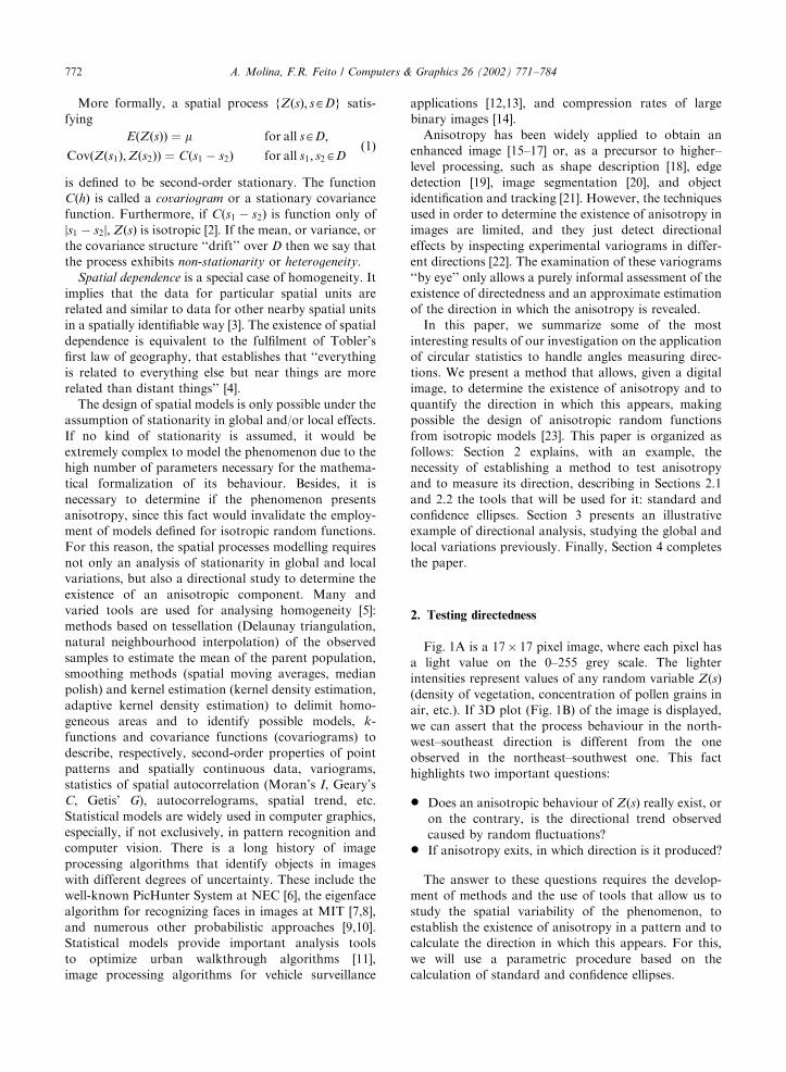
When analysing the standard ellipse obtained (Fig. 2),

we observe that the assumption of normality is reason-

able, so that, a confidence ellipse is applicable to it. We

want to determine the confidence ellipse at a level of

significance a ¼ 5% from mean vectors shown in Table

2. As a first step, we calculate T2ð0:05Þ using Eq. (20).

From a table of the F-distribution we read F2;4 ¼ 6:94:Hence, T2ð0:05Þ ¼ 17:35: From Eqs. (22) and (24) we

obtain the parameters D ¼ 0:00007; a ¼ 0:221 and b ¼0:038 (Table 3). Our confidence ellipse (Fig. 3) is

somewhat bigger than the standard ellipse (dashed

curve). Since the confidence ellipse does not contain

the origin inside, ð %x; %yÞ differs significantly from the

origin. Therefore, the mean vectors are oriented as a

group, the direction being at c ¼ 321:

3. An illustrative example

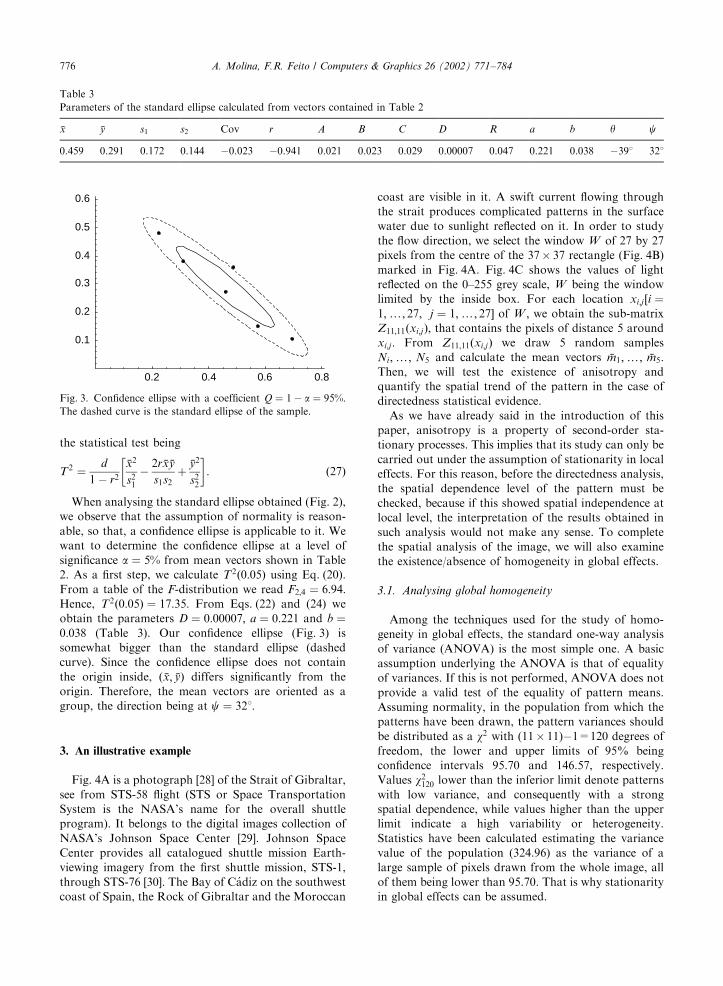
Fig. 4A is a photograph [28] of the Strait of Gibraltar,

see from STS-58 flight (STS or Space Transportation

System is the NASA’s name for the overall shuttle

program). It belongs to the digital images collection of

NASA’s Johnson Space Center [29]. Johnson Space

Center provides all catalogued shuttle mission Earth-

viewing imagery from the first shuttle mission, STS-1,

through STS-76 [30]. The Bay of C!adiz on the southwest

coast of Spain, the Rock of Gibraltar and the Moroccan

coast are visible in it. A swift current flowing through

the strait produces complicated patterns in the surface

water due to sunlight reflected on it. In order to study

the flow direction, we select the window W of 27 by 27

pixels from the centre of the 37� 37 rectangle (Fig. 4B)

marked in Fig. 4A. Fig. 4C shows the values of light

reflected on the 0–255 grey scale, W being the window

limited by the inside box. For each location xi;j ½i ¼1;y; 27; j ¼ 1;y; 27� of W ; we obtain the sub-matrix

Z11;11ðxi;jÞ; that contains the pixels of distance 5 around

xi;j : From Z11;11ðxi;jÞ we draw 5 random samples

Ni;y; N5 and calculate the mean vectors %m1;y; %m5:Then, we will test the existence of anisotropy and

quantify the spatial trend of the pattern in the case of

directedness statistical evidence.

As we have already said in the introduction of this

paper, anisotropy is a property of second-order sta-

tionary processes. This implies that its study can only be

carried out under the assumption of stationarity in local

effects. For this reason, before the directedness analysis,

the spatial dependence level of the pattern must be

checked, because if this showed spatial independence at

local level, the interpretation of the results obtained in

such analysis would not make any sense. To complete

the spatial analysis of the image, we will also examine

the existence/absence of homogeneity in global effects.

3.1. Analysing global homogeneity

Among the techniques used for the study of homo-

geneity in global effects, the standard one-way analysis

of variance (ANOVA) is the most simple one. A basic

assumption underlying the ANOVA is that of equality

of variances. If this is not performed, ANOVA does not

provide a valid test of the equality of pattern means.

Assuming normality, in the population from which the

patterns have been drawn, the pattern variances should

be distributed as a w2 with (11� 11)�1=120 degrees of

freedom, the lower and upper limits of 95% being

confidence intervals 95.70 and 146.57, respectively.

Values w2120 lower than the inferior limit denote patterns

with low variance, and consequently with a strong

spatial dependence, while values higher than the upper

limit indicate a high variability or heterogeneity.

Statistics have been calculated estimating the variance

value of the population (324.96) as the variance of a

large sample of pixels drawn from the whole image, all

of them being lower than 95.70. That is why stationarity

in global effects can be assumed.

0.2 0.4 0.6 0.8

0.1

0.2

0.3

0.4

0.5

0.6

Fig. 3. Confidence ellipse with a coefficient Q ¼ 1� a ¼ 95%:The dashed curve is the standard ellipse of the sample.

Table 3

Parameters of the standard ellipse calculated from vectors contained in Table 2

%x %y s1 s2 Cov r A B C D R a b y c

0.459 0.291 0.172 0.144 �0.023 �0.941 0.021 0.023 0.029 0.00007 0.047 0.221 0.038 �391 321


3.2. Analysing local spatial dependence

The analysis of spatial dependence is carried out by

the exploration of the spatial covariance structure of the

pattern. For that, the most commonly used technique is

the autocorrelation test based on any of the statistics

designed for it, such Moran’s I ; Geary’s C; Getis’ G or

Lagrange multiplier [31]. Moran’s I is the most widely

used of them. For a matrix Zn;n; these statistics at k lag is

estimated as

I ðkÞ ¼nPn

i¼1

Pnj¼1 d

ðkÞi;j ðzi � %zÞðzj � %zÞPn

i¼1ðzi � %zÞ2P

iaj

PdðkÞi;j

: ð28Þ

Fig. 4. (A) Strait of Gibraltar, seen from STS-58 flight. (B) Window of 37� 37 pixels marked in the image. (C) Values of reflected light

on the 0–255 grey scale. W is the squared window of 27� 27 pixels. The dashed rectangle is the window of locations fxi;j ; i ¼2;y; 17; j ¼ 21;y; 26g used in Tables 5 and 7.


The expected value EðIÞ and variance VarðIÞ are

EðIÞ ¼ �1

n � 1; VarðIÞ ¼

n2S1 � nS2 þ 3S20

S20ðn

2 � 1Þ; ð29Þ

where

S0 ¼1

2

Xn

i¼1

Xn

j¼1

ðdi;j þ dj;iÞ2;

S1 ¼Xn

i¼1

Xn

i¼1

di;j þXn

j¼1

dj;i

!2

: ð30Þ

Here, dðkÞi;j denotes the spatial connection between the ith

and jth cells. Although the correlation coefficients are

usually restricted to (�1, 1) range, this is not Moran’s I

case. In order to force the (�1, 1) range, I must be

divided by a correction factor c:

cðkÞ ¼nP

iaj

PdðkÞi;j

Pni¼1

Pnj¼1 d

ðkÞi;j ðzi � %zÞ

� �2Pn

i¼1ðzi � %zÞ2

0B@

1CA

1=2

: ð31Þ

A larger positive value is associated with a clustered

pattern. On the contrary, a negative value different from

zero implies a scattered pattern. Values near to zero

represent lack of spatial dependence and consequently

they are associated with random spatial patterns. If

Eq. (28) is observed, we can see how I is not a sound

measure for patterns in which all their cells have the

same value, since we find 00indeterminations.

A common practice for exploring spatial dependence

is estimating spatial correlation at different lags for the

construction of a correlogram where I ðkÞ is plotted

against the k lag. The observation of this correlogram,

and specially its peaks, allows us to obtain information

about the level and direction of autocorrelation and the

lags on which this reaches its maximum and minimum

values. Another method for analysing the variation of

the spatial dependence level of a pattern is calculating

I 1ð Þ from the matrices fZ2kþ1;2kþ1ðxi;j ; kÞ; k ¼ 1;y; 5g;where Z2kþ1;2kþ1ðxi;j ; kÞ is the matrix that contains the

pixels of distance k around the xi;j : For each location xi;j ;we will obtain 5 indexes fI ð1Þðxi;j ; kÞ; k ¼ 1;y; 5g of

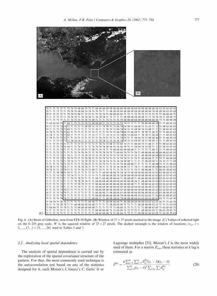
autocorrelation. Table 5 shows these indexes for the

window of locations fxi;j ; i ¼ 2;y; 17; j ¼ 21;y; 26g(dashed rectangle in Fig. 4C). Each one of these groups

of 5 indexes is fitted, after removing the detected

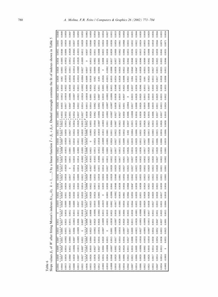
indeterminations, by a linear function #I ¼ b1 þ b2x:The values of the slope b2 for each location in W are

represented in Table 6.

From Eq. (29) the expected indexes fEðIðkÞÞ; k ¼1y5g ¼ �1

8; �124; �148; �180; �1120

# $are obtained. Table 4 shows

the parameters of the linear fit of these values and their

confidence intervals calculated with a signification a ¼5%: Among the 729 cells, only 15 of them (Fig. 5) can be

considered spatially independent, since they present

values of slope out of the confidence interval.

3.3. Analysing directedness

As was said in Section 2, the first step when analysing

directedness is testing if there is statistical evidence of

anisotropic behaviour. For each Z11;11ðxi;jÞ of W ; wedraw 5 random samples Ni;y; N5 and calculate its

mean vectors f %mi; i ¼ 1;y; 5g by applying Eqs. (4) and

(6). The length r and mean angle %F of the cells belonging

to the rectangle dashed in Fig. 4C are shown in Table 7.

After obtaining the mean vectors of each cell of W ; wedetermine the parameters of the confidence ellipse that

allow us to obtain the statistic T2 (Eq. (27)) and we will

apply condition Eq. (26) for testing the anisotropy. All

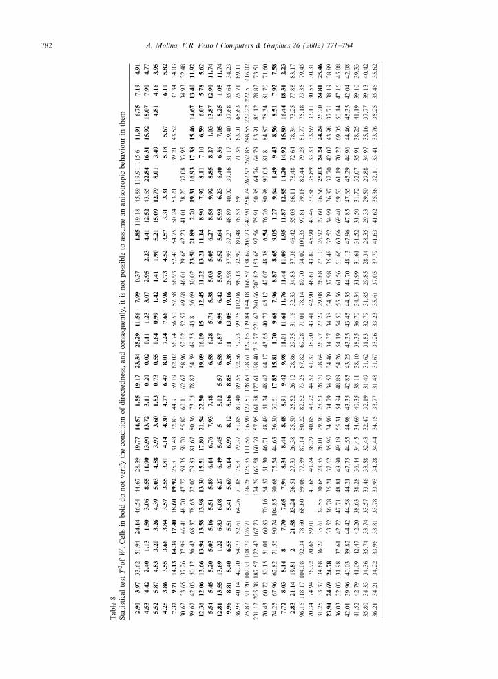
confidence ellipses have been calculated with d ¼ 5

vectors, so that the critical value T2ð0:05Þ (Eq. (20)) forall cells is 25.47. Table 8 shows the values of the statistics

Fig. 5. Behaviour of W cells. The symbols have the following

interpretation: * Homogeneity in global effects and lack of

spatial dependence in local ones. K Homogeneity in global

effects and spatial dependence in local ones with isotropic

behaviour. Arrows represent homogeneity in global effects and

spatial dependence in local ones, with anisotropic behaviour in

direction c calculated with d ¼ 5 mean vectors.

Table 4

Fit parameters of the expected indexes EðIðkÞÞ; k ¼ 1;y; 5 ¼�18; �124;�148;�180; �1120

# $by a linear function #I ¼ b1 þ b2h

Best Fit Parameters

Parameter Estimate Standard error Confidence interval

1 �0.1204 0.0300 (�0.0216, �0.0250)

X 0.0262 0.0090 (�0.0025, 0.0550)

Note: Confidence intervals have been calculated with a

significance a ¼ 5%:


Table

5

Moran’sindexes

Iðx

i;j;

kÞ;

k¼

1;y

;5forthewindow

oflocations

xi;

j;i¼

2;y

;17;

j¼

21;y

;26(dashed

rectangle

inFig.4C)

�0.0130

�0.0004

0.0016

0.0036

�0.0033

�0.0058

�0.0096

�0.0038

0.0020

�0.0055

0.0100

�0.0110

0.0100

0.0097

�0.0029

0.0031

0.0024

0.0066

0.0110

0.0120

0.0140

0.0120

0.0120

0.0070

�0.0009

0.0110

0.0150

0.0110

0.0110

0.0120

0.0016

0.0038

0.0060

0.0087

0.0110

0.0130

0.0100

0.0090

0.0085

0.0076

0.0065

0.0080

0.0091

0.0079

0.0053

0.0037

0.0074

0.0068

0.0074

0.0078

0.0093

0.0087

0.0085

0.0067

0.0061

0.0062

0.0076

0.0071

0.0068

0.0070

0.0063

0.0073

0.0080

0.0110

0.0082

0.0087

0.0079

0.0080

0.0081

0.0081

0.0059

0.0062

0.0073

0.0077

0.0077

0.0073

0.0083

0.0086

0.0095

0.0110

�0.0074

0.0024

Indet.

Indet.

�0.0009

0.0016�

0.0038

0.0038

�0.0073

�0.0029

0.0120

�0.0069

0.0100

0.0130

�0.0150

�0.0034

0.0008

0.0023

0.0066

0.0002

�0.0003

�0.0001

�0.0009

�0.0018

�0.0009

0.0062

0.0120

0.0097

0.0095

0.0110

0.0009

0.0023

0.0034

0.0062

0.0084

0.0098

0.0074

0.0075

0.0068

0.0055

0.0058

0.0087

0.0099

0.0090

0.0064

0.0027

0.0042

0.0024

0.0062

0.0068

0.0084

0.0076

0.0073

0.0062

0.0059

0.0058

0.0073

0.0063

0.0057

0.0054

0.0040

0.0049

0.0055

0.0100

0.0068

0.0071

0.0060

0.0061

0.0060

0.0063

0.0050

0.0056

0.0057

0.0061

0.0052

0.0044

0.0055

0.0059

0.0075

0.0095

�0.0230

0.0017

Indet.

Indet.

Indet.

Indet.

0.0016

�0.0073

�0.0007

��0.0008

0.0030

�0.0034

00.0093

�0.0072

�0.0150

0.0021

0.0021

0.0047

00.0018

0.0034

0.0047

0.0028

�0.0009

0.0033

0.0095

0.0077

0.0110

0.0110

0.0029

0.0021

0.0031

0.0044

0.0036

0.0036

0.0014

0.0008

�0.0001

0.0006

0.0030

0.0072

0.0065

0.0071

0.0053

0.0032

0.0050

0.0019

0.0056

0.0055

0.0066

0.0061

0.0061

0.0050

0.0058

0.0054

0.0072

0.0064

0.0063

0.0055

0.0037

0.0034

0.0025

0.0069

0.0059

0.0061

0.0049

0.0049

0.0053

0.0060

0.0050

0.0063

0.0058

0.0061

0.0048

0.0033

0.0043

0.0044

0.0066

0.0092

�0.0110

0.0047

�0.0031

0.0008

Indet.

Indet.

0.0016

�0.0067

�0.0029

0.0016

�0.0009

�0.0007

�0.0008

�0.0017

�0.006

�0.0058

0.0069

0.0092

0.0097

0.0064

0.0051

0.0009

0.0016

0.0001

0.0028

0.0009

0.0050

0.0047

0.0042

0.0052

0.0017

�0.0005

0.0064

0.0063

0.0062

0.0072

0.0055

0.0046

0.0021

0.0050

0.0050

0.0059

0.0044

0.0069

0.0056

0.0033

0.0044

0.0016

0.0042

0.0026

0.0026

0.0028

0.0032

0.0027

0.0044

0.0040

0.0067

0.0058

0.0063

0.0050

0.0035

0.0039

0.0022

0.0064

0.0052

0.0050

0.0039

0.0040

0.0049

0.0059

0.0049

0.0064

0.0061

0.0061

0.0056

0.0041

0.0042

0.0041

0.0058

0.0078

00.0087

0.0031

0.0058

�0.0008

Indet.

�0.0008

�0.0031

�0.0029

0.0038

�0.0009

0.003

0.0057

�0.0008

Indet.

�0.0017

0.0070

0.0110

0.0100

0.0091

0.0095

0.0018

�0.0002

0.0003

0.0044

0.0023

0.0062

0.0073

0.0035

0.0035

�0.0006

�0.0030

0.0066

0.0065

0.0066

0.0073

0.0044

0.0040

0.0044

0.0086

0.0049

0.0073

0.0064

0.0073

0.0063

0.0009

0.0026

�0.0013

0.0042

0.0044

0.0045

0.0043

0.0047

0.0046

0.0065

0.0055

0.0076

0.0069

0.0067

0.0059

0.0048

0.0048

0.0036

0.0067

0.0050

0.0044

0.0035

0.0035

0.0045

0.0057

0.0045

0.0058

0.0057

0.0058

0.0055

0.0047

0.0045

0.0045

0.0058

0.0074

�0.0059

0.0031

�0.0050

0.0052

0.0016

Indet.

�0.0008

�0.0031

�0.0012

�0.0034

0.0060

0.0026

0.0026

0.0025

�0.0017

�0.0060

0.0021

0.0062

0.0077

0.0069

0.0086

0.0022

0.0027

0.0071

0.0091

0.0055

0.0130

0.0130

0.0100

0.0110

�0.0027

�0.0039

0.0053

0.0055

0.0061

0.0066

0.0040

0.0031

0.0053

0.0081

0.0060

0.0086

0.0079

0.0088

0.0092

0.0029

0.0041

0.0022

0.0062

0.0074

0.0073

0.0068

0.0063

0.0060

0.0076

0.0061

0.0072

0.0062

0.0067

0.0074

0.0060

0.0054

0.0029

0.0053

0.0056

0.0059

0.0056

0.0054

0.0062

0.0073

0.0060

0.0070

0.0067

0.0068

0.0059

0.0044

0.0041

0.0043

0.0056

0.0070


Table

6

Slopevalues

b 2of

Wafter

fittingMoran’sindexes

Iðx

i;j;

kÞ;

k¼

1;y

;5byalinearfunction

# I¼

b 1þ

b 2x:Dashed

rectangle

containsthefitofindexes

shownin

Table

5

0.00

41

0.00

40

0.00

09

0.00

07

0.00

10

0.00

11

0 -0

.001

9 0.

0032

0.

0046

0.

0036

-0

.000

4 0.

0023

0.

0022

0.

0018

0.

0031

0.

0033

-0

.000

1 -0

.002

6 -0

.002

2 0.

0023

0.

0039

0.

0028

0.

0034

0.

0055

0.

0043

0.

0048

0.00

43

0.00

47

0.00

20

0.00

11

0.00

05

0.00

17

0.00

23

0.00

26

0.00

19

0.00

19

0.00

23

-0.0

013

0.00

33

-0.0

008

-0.0

007

0.00

31

0.00

22

0.00

33

0.00

35

-0.0

012

0.00

10

0.00

2 0.

0003

-0

.000

5 0.

0040

0.

0029

0.

0049

0.00

13

0.00

34

0.00

14

-0.0

002

0.00

15

0.00

21

0.00

16

0.00

09

0.00

11

0.00

34

0.00

18

-0.0

020

0.00

18

-0.0

015

-0.0

020

0.00

50

0.00

33

0.00

32

0.00

17

-0.0

018

0.00

22

-0.0

018

-0.0

023

-0.0

032

0.00

06

0.00

34

0.00

58

0.00

12

0.00

60

0.00

12

0.00

04

0.00

17

0.00

15

0.00

12

0.00

08

0.00

30

0.00

21

0.00

17

0 0.

0011

0.

0001

-0

.001

7 0.

0027

0.

0052

0.

0055

0.

0047

-0

.000

6 0.

0030

-0

.003

4 -0

.001

1 -0

.001

2 -0

.002

8 0.

0041

0.

0047

0.00

08

0.00

30

-0.0

006

0.00

07

0.00

06

-0.0

003

0.00

13

0.00

09

0.00

30

0.00

22

0.00

14

0.00

14

0.00

10

0.00

09

0.00

10

0.00

24

0.00

34

0.00

540.

0049

-0

.000

7 0.

0022

-0

.003

6 -0

.001

4 -0

.001

6 -0

.004

5 0.

0037

0.

0049

0.00

13

0.00

07

-0.0

015

-0.0

005

-0.0

009

0.00

06

0.00

12

0.00

17

0.00

23

0.00

20

0.00

09

0.00

14

0.00

14

-0.0

001

0.00

12

0.00

20

0.00

28

0.00

37

0.00

22

-0.0

021

0.00

13

-0.0

024

-0.0

009

-0.0

028

-0.0

033

0.00

36

0.00

50

0.00

21

0.00

27

0.00

07

0.00

21

0 0.

0007

0.

0018

0.

0019

0.

0019

0.

0014

0.

0021

-0

.000

7 -0

.000

2 -0

.000

1 -0

.000

2 0.

0020

0.

0035

0.

0027

0.

0014

-0

.002

4 -0

.000

2 -0

.000

4 0.

0027

-0

.000

9 0.

0012

0.

0028

0.

0050

0.00

36

0.00

30

-0.0

001

0.00

04

0.00

20

0.00

08

0.00

12

0.00

17

0.00

15

0.00

08

0.00

29

-0.0

026

-0.0

023

0.00

06

-0.0

010

0.00

06

0.00

52

0.00

30

0.00

13

-0.0

018

0.00

04

0.00

09

0.00

37

0 0.

0037

0.

0034

0.

0063

0.00

33

0.00

26

0.00

19

0.00

04

0.00

23

0.00

07

0.00

08

0.00

25

0.00

28

0.00

22

0.00

46

-0.0

027

-0.0

015

0.00

21

0 -0

.000

1 0.

0055

0.

0024

0.

0014

0.

0001

0.

0026

0.

0018

0.

0032

0.

0013

0.

0034

0.

0040

0.

0058

0.00

29

0.00

36

0.00

27

0.00

10

-0.0

002

0.00

20

-0.0

006

0.00

19

0.00

24

0.00

13

0.00

33

-0.0

001

-0.0

015

0.00

13

0.00

24

0.00

24

0.00

44

0.00

62

0.00

62

0.00

33

0.00

12

0.00

2 0.

0009

0.

0002

0.

0011

0.

0028

0.

0034

0.00

12

0.00

24

0.00

27

0.00

16

-0.0

016

0.00

26

-0.0

002

-0.0

009

0.00

05

0.00

13

0.00

18

0.00

15

-0.0

006

-0.0

012

-0.0

018

-0.0

010

-0.0

007

-0.0

006

0.00

02

0.00

07

0.00

11

-0.0

01

0.00

04

0.00

05

0.00

08

0.00

34

0.00

47

-0.0

002

0.00

16

0.00

04

0.00

20

-0.0

007

-0.0

009

0.00

13

-0.0

019

0 0.

0019

0.

0024

0.

0014

0.

0011

-0

.000

2 -0

.000

9 -0

.001

1 -0

.000

3 0.

0010

-0

.000

3 0.

0010

0.

0005

-0

.002

6 0

0.00

08

0.00

25

0.00

24

0.00

34

-0.0

010

0.00

34

-0.0

008

0.00

15

0 -0

.003

1 0.

0019

0.

0002

0.

0003

0.

0030

0.

0030

0.

0027

0.

0013

0.

0003

-0

.000

1 0.

0001

0.

0011

-0

.000

2 -0

.000

7 -0

.000

2 -0

.000

1 -0

.001

5 -0

.000

2 0.

0021

0.

0030

0.

0028

0.

0027

-0.0

008

0.00

40

-0.0

007

0.00

15

0.00

01

-0.0

030

0.00

21

0.00

02

-0.0

006

0.00

41

0.00

28

0.00

28

0.00

22

0.00

17

0.00

24

0.00

11

0.00

04

-0.0

007

-0.0

007

-0.0

006

0.00

15

0.00

19

0.00

08

0.00

17

0.00

39

0.00

36

0.00

15

0.00

10

0.00

20

0.00

02

0.00

17

-0.0

008

-0.0

007

0.00

16

-0.0

017

-0.0

002

0.00

48

0.00

40

0.00

29

0.00

16

0.00

17

0.00

27

0.00

22

0.00

07

0.00

27

0.00

38

0.00

38

0.00

48

0.00

34

0.00

38

0.00

57

0.00

60

0.00

54

0.00

19

0.00

43

0.00

09

0.00

20

0.00

14

-0.0

016

0.00

28

0.00

05

-0.0

001

0.00

19

0.00

38

0.00

61

0.00

26

0.00

17

0.00

13

0.00

15

0.00

36

0.00

23

0.00

270.

0013

0.

0019

0.

0035

0.

0028

0.

0026

0.

0037

0.

0062

0.

0061

0.

0058

0.00

34

0.00

06

0.00

24

0.00

16

-0.0

007

0.00

20

0.00

04

0.00

34

0.00

61

0.00

56

0.00

56

0.00

27

0.00

21

0.00

16

0.00

09

0.00

32

0.00

43

0.00

500.

0051

0.

0037

0.

0025

0.

0008

0.

0022

0.

0050

0.

0066

0.

0068

0.

0058

0.00

42

0.00

22

0.00

13

0.00

27

0.00

17

0.00

20

0.00

25

0.00

52

0.00

66

0.00

68

0.00

45

0.00

25

0.00

27

0.00

26

0.00

11

0.00

2 0.

0037

0.

0006

-0

.000

4 0

0.00

06

0.00

21

0.00

42

0.00

42

0.00

53

0.00

33

0.00

33

0.00

07

0.00

21

0.00

16

0.00

08

0.00

09

0.00

13

0.00

30

0.00

44

0.00

50

0.00

47

0.00

42

0.00

27

0.00

27

0.00

16

0.00

19

0.00

04

0.00

15

-0.0

008

0.00

17

0.00

33

0.00

37

0.00

4 0.

0040

0.

0048

0.

0036

0.

0032

0.

0035

0.00

14

0.00

06

0.00

09

-0.0

010

-0.0

021

-0.0

026

-0.0

001

0.00

35

0.00

39

0.00

39

0.00

31

0.00

25

0.00

36

0.00

29

0.00

29

0.00

06

0.00

19

0.00

16

0.00

08

0.00

28

0.00

36

0.00

19

0.00

47

0.00

25

0.00

23

0.00

22

0.00

44

0.00

06

0.00

20

-0.0

006

-0.0

016

0.00

27

-0.0

003

-0.0

008

0.00

30

0.00

31

0.00

38

0.00

35

0.00

28

0.00

32

0.00

36

0.00

12

0.00

31

0.00

35

0.00

30

0.00

26

0.00

20

0.00

46

0.00

18

0.00

38

0.00

46

0.00

13

0.00

24

0.00

30

0.00

22

0.00

08

0.00

02

-0.0

032

-0.0

005

-0.0

009

-0.0

003

0.00

29

0.00

28

0.00

24

0.00

23

0.00

32

0.00

32

0.00

17

0.00

27

0.00

26

0.00

26

0.00

28

0.00

19

0.00

15

0.00

15

0.00

1 0.

0033

0.

0049

0.

0014

0.

0033

0.

0018

0.00

21

0.00

26

0.00

18

-0.0

010

-0.0

007

-0.0

011

0.00

17

0.00

38

0.00

28

0.00

21

0.00

21

0.00

29

0.00

25

0.00

20

0.00

08

0.00

13

0.00

21

0.00

16

0.00

08

0.00

18

0.00

17

0.00

24

0.00

39

0.00

42

0.00

08

0.00

18

0.00

29

0.00

33

0.00

17

0.00

14

0.00

30

0.00

34

0.00

31

0.00

13

0.00

27

0.00

29

0.00

20

0.00

23

0.00

23

0.00

20

0.00

12

0.00

13

0.00

03

0.00

33

0.00

06

0.00

19

0.00

19

0.00

10

0.00

13

0.00

27

0.00

28

0.00

24

0.00

18

0.00

36

0.00

47

0.00

14

0.00

28

0.00

54

0.00

52

0.00

47

0.00

51

0.00

33

0.00

28

0.00

23

0.00

32

0.00

28

0.00

27

0.00

20

0.00

06

0.00

15

0.00

19

0.00

17

0.00

11

0.00

29

0.00

25

0.00

17

0.00

15

0.00

25

0.00

50

0.00

44

0.00

44

0.00

34

0.00

14

0.00

13

0.00

38

0.00

53

0.00

37

0.00

25

0.00

31

0.00

17

0.00

30

0.00

21

0.00

21

0.00

22

0.00

16

0.00

06

0.00

16

0.00

26

0.00

17

0.00

13

0.00

33

0.00

38

0.00

28

0.00

35

0.00

25

0.00

45

0.00

74

0.00

33

-0.0

002

-0.0

003

0 0.

0033

0.

0025

0.

0001

0.

0015

0.

0004

0.

0018

0.

0016

0.

0005

0.

0001

0.

0002

0.

0001

0.

0019

0.

0006

0.

0058

0.

0010

0.

0024

0.

0022

0.

0033

0.

0008

0.

0013

0.

0046

0.

0035

0.

0071

0.

0034


Table

7

Meanvectors

(length

randmeanangle

% F)ofcellsbelongingto

rectangle

dashed

inFig.4C

(0.011,226)(0.007,241)(0.004,236)(0.002,158)(0.007,109)(0.012,107)(0.015,111)(0.012,107)(0.007,119)(0.004,140)(0.004,7)

(0.006,348)(0.002,289)(0.004,158)(0.005,108)(0.007,68)

(0.006,36)

(0.011,51)

(0.018,49)

(0.022,55)

(0.026,62)

(0.026,68)

(0.026,72)

(0.026,78)

(0.025,78)

(0.024,64)

(0.024,58)

(0.025,53)

(0.025,57)

(0.024,62)

(0.024,67)

(0.024,67)

(0.032,91)

(0.034,88)

(0.037,85)

(0.041,81)

(0.041,83)

(0.042,83)

(0.042,85)

(0.043,86)

(0.044,83)

(0.044,81)

(0.043,79)

(0.042,80)

(0.040,77)

(0.037,77)

(0.033,80)

(0.029,85)

(0.040,244)(0.035,247)(0.032,246)(0.030,243)(0.025,244)(0.022,240)(0.020,238)(0.017,246)(0.015,248)(0.014,244)(0.015,239)(0.016,247)(0.018,246)(0.021,252)(0.023,251)(0.026,245)

(0.090,244)(0.084,245)(0.081,245)(0.077,245)(0.073,245)(0.068,245)(0.065,246)(0.063,246)(0.062,247)(0.061,246)(0.061,246)(0.061,245)(0.062,247)(0.064,246)(0.066,245)(0.068,244)

(0.007,174)(0.005,145)(0.005,145)(0.005,145)(0.005,155)(0.005,175)(0.004,205)(0.003,240)(0.003,227)(0.003,199)(0.001,30)

(0.003,43)

(0.002,108)(0.005,161)(0.003,162)(0.002,105)

(0.005,292)(0.004,304)(0.005,342)(0.005,1)

(0.006,23)

(0.006,34)

(0.006,40)

(0.005,42)

(0.005,29)

(0.007,8)

(0.008,3)

(0.010,0)

(0.009,1)

(0.007,3)

(0.006,11)

(0.007,16)

(0.010,112)(0.011,106)(0.012,101)(0.013,91)

(0.014,92)

(0.015,94)

(0.016,97

(0.016,98)

(0.016,92)

(0.016,85)

(0.015,80)

(0.014,80)

(0.014,73)

(0.014,73)

(0.014,76)

(0.012,84)

(0.023,217)(0.020,219)(0.019,218)(0.019,217)(0.017,217)(0.017,214)(0.017,212)(0.015,212)(0.013,211)(0.012,208)(0.012,207)(0.011,213)(0.012,215)(0.012,223)(0.013,225)(0.016,221)

(0.075,239)(0.072,239)(0.071,240)(0.069,239)(0.067,239)(0.064,240)(0.062,241)(0.061,241)(0.060,241)(0.060,241)(0.059,241)(0.059,240)(0.059,241)(0.060,241)(0.061,240)(0.061,240)

(0.006,202)(0.003,220)(0.003,220)(0.003,220)(0.003,220)(0.003,220)(0.003,240)(0.003,249)(0.003,231)(0.003,220)(0.002,253)(0.001,323)(0.001,270)(0.003,225)(0.004,246)(0.004,246)

(0.005,278)(0.005,277)(0.006,291)(0.006,286)(0.007,280)(0.007,282)(0.008,286)(0.008,290)(0.008,294)(0.008,303)(0.008,311)(0.009,314)(0.008,308)(0.008,304)(0.008,296)(0.009,300)

(0.007,204)(0.006,208)(0.006,209)(0.004,213)(0.004,207)(0.004,197)(0.005,194)(0.005,196)(0.004,202)(0.003,224)(0.003,246)(0.003,251)(0.003,271)(0.003,273)(0.002,279)(0.002,254)

(0.024,221)(0.023,222)(0.022,221)(0.021,221)(0.020,221)(0.020,221)(0.020,221)(0.019,222)(0.019,223)(0.018,224)(0.018,225)(0.017,228)(0.017,227)(0.016,230)(0.017,229)(0.018,223)

(0.053,226)(0.052,227)(0.051,227)(0.050,227)(0.049,228)(0.047,229)(0.046,229)(0.045,229)(0.044,229)(0.044,229)(0.043,229)(0.043,229)(0.043,230)(0.043,230)(0.044,229)(0.045,228)

(0.006,232)(0.006,252)(0.007,254)(0.007,252)(0.007,252)(0.007,252)(0.006,257)(0.006,256)(0.006,252)(0.007,257)(0.007,261)(0.007,267)(0.006,270)(0.007,265)(0.008,266)(0.009,261)

(0.009,273)(0.010,275)(0.011,280)(0.011,278)(0.012,275)(0.012,276)(0.011,277)(0.011,280)(0.012,282)(0.011,284)(0.011,288)(0.011,290)(0.011,288)(0.011,289)(0.011,285)(0.012,286)

(0.010,215)(0.010,216)(0.010,217)(0.010,222)(0.011,225)(0.011,227)(0.011,231)(0.011,237)(0.011,243)(0.010,246)(0.010,247)(0.010,246)(0.010,245)(0.010,243)(0.009,243)(0.009,241)

(0.027,224)(0.026,225)(0.026,225)(0.025,225)(0.024,226)(0.024,227)(0.024,228)(0.024,228)(0.023,229)(0.023,230)(0.023,232)(0.023,233)(0.022,234)(0.022,235)(0.022,235)(0.022,230)

(0.048,223)(0.047,223)(0.046,224)(0.045,224)(0.045,225)(0.044,226)(0.043,226)(0.043,225)(0.042,225)(0.042,225)(0.041,224)(0.040,224)(0.04,224)

(0.039,223)(0.040,222)(0.040,220)

(0.007,248)(0.007,258)(0.008,259)(0.009,256)(0.009,254)(0.009,254)(0.009,256)(0.008,255)(0.008,257)(0.008,262)(0.009,260)(0.008,260)(0.008,264)(0.007,265)(0.007,265)(0.008,262)

(0.011,269)(0.012,272)(0.012,275)(0.013,273)(0.013,271)(0.013,271)(0.013,272)(0.013,275)(0.014,277)(0.014,276)(0.014,277)(0.014,277)(0.014,278)(0.013,279)(0.013,278)(0.013,278)

(0.013,222)(0.013,223)(0.013,224)(0.012,227)(0.012,229)(0.013,229)(0.013,233)(0.013,237)(0.012,239)(0.012,239)(0.012,240)(0.012,240)(0.012,238)(0.012,238)(0.011,239)(0.011,240)

(0.027,220)(0.027,221)(0.027,221)(0.027,222)(0.027,224)(0.027,226)(0.027,227)(0.027,228)(0.026,229)(0.026,230)(0.025,230)(0.025,228)(0.025,227)(0.024,226)(0.024,224)(0.023,220)

(0.043,217)(0.042,218)(0.042,219)(0.041,219)(0.041,220)(0.040,221)(0.040,221)(0.040,221)(0.040,221)(0.040,222)(0.039,222)(0.039,222)(0.038,222)(0.038,222)(0.038,221)(0.039,220)

(0.007,249)(0.007,255)(0.007,257)(0.007,252)(0.008,249)(0.008,249)(0.008,251)(0.008,251)(0.008,258)(0.008,263)(0.009,257)(0.009,252)(0.008,255)(0.007,260)(0.007,256)(0.006,255)

(0.011,266)(0.011,268)(0.011,270)(0.011,269)(0.011,266)(0.012,266)(0.012,267)(0.012,272)(0.013,274)(0.013,273)(0.013,272)(0.013,270)(0.012,271)(0.011,273)(0.011,275)(0.011,275)

(0.013,222)(0.013,225)(0.014,228)(0.014,231)(0.014,233)(0.014,233)(0.014,235)(0.014,237)(0.014,237)(0.014,237)(0.014,238)(0.013,238)(0.014,234)(0.013,232)(0.013,231)(0.012,229)

(0.025,211)(0.025,212)(0.025,213)(0.024,214)(0.024,216)(0.024,218)(0.024,219)(0.024,220)(0.024,220)(0.024,220)(0.023,221)(0.023,219)(0.023,219)(0.023,218)(0.023,218)(0.023,217)

(0.042,212)(0.042,212)(0.041,213)(0.041,213)(0.041,214)(0.040,216)(0.040,217)(0.040,217)(0.040,218)(0.040,219)(0.040,219)(0.039,220)(0.039,220)(0.039,220)(0.040,220)(0.040,219)


Table

8

Statisticaltest

T2of

W:Cellsin

bold

donotverifytheconditionofdirectedness,andconsequently,itisnotpossible

toassumeananisotropic

behaviourin

them

2.90

3.97

33.62

51.94

24.14

46.54

44.67

28.39

19.77

14.57

1.55

19.17

23.34

25.29

11.56

7.99

0.37

1.85119.18

45.89119.91115.6

11.91

6.75

7.19

4.91

4.53

4.42

2.40

1.13

1.50

3.06

8.55

11.90

13.90

13.72

3.11

0.20

0.02

0.11

1.23

3.07

2.95

2.23

4.41

12.52

43.65

22.84

16.31

15.92

18.07

7.90

4.77

5.52

5.87

4.83

3.20

3.26

4.39

5.03

4.58

3.97

3.60

1.83

0.73

0.55

0.64

0.99

1.42

1.41

1.90

5.21

15.09

12.79

8.01

3.49

4.81

4.16

3.95

4.25

3.86

3.55

3.66

3.84

3.57

3.55

3.81

4.14

4.30

4.77

6.47

8.01

7.24

7.66

9.96

6.73

4.52

3.57

3.31

3.31

5.18

5.67

6.10

5.82

7.37

9.71

14.13

14.39

17.40

18.60

19.92

25.81

31.48

32.83

44.91

59.19

62.02

56.74

56.50

57.58

56.93

52.40

54.75

50.24

53.21

39.21

43.52

37.34

34.03

30.62

33.65

37.26

37.98

46.41

48.70

47.72

59.35

58.70

55.82

60.11

62.67

58.96

52.02

52.57

49.68

46.01

39.65

42.23

41.01

38.23

37.08

33.95

34.93

32.48

39.67

42.03

50.12

56.43

68.37

78.63

72.02

79.83

81.67

80.36

73.05

78.87

54.59

49.35

45.8

36.69

30.02

23.50

21.89

2.20

19.31

16.93

17.38

15.46

14.67

13.40

11.92

12.36

12.06

13.66

13.94

13.58

13.98

13.30

15.51

17.80

21.54

22.50

19.09

16.09

15

12.45

11.22

13.21

11.14

8.90

7.92

8.11

7.10

6.59

6.07

5.78

5.62

5.54

5.45

5.20

5.03

5.16

5.51

5.89

6.14

6.76

7.93

7.48

6.58

6.28

5.74

5.38

5.03

5.05

6.27

8.58

9.92

8.85

8.27

1.03

13.87

12.90

11.74

12.81

13.55

13.69

1.22

6.83

6.08

6.27

6.49

5.45

55.02

5.57

6.58

6.87

6.98

6.42

5.90

5.52

5.64

5.93

6.23

6.40

6.36

7.05

8.25

1.05

11.74

9.96

8.81

8.40

6.55

5.51

5.41

5.69

6.14

6.99

8.12

8.66

8.85

9.38

11

13.05

19.16

26.98

37.93

37.27

48.89

40.02

39.16

31.17

29.40

37.68

35.64

34.23

36.98

40.14

42.70

54.73

52.61

64.26

71.85

75.81

79.37

81.85

80.40

89.55

92.56

79.93

99.75102.06

96.13

92.92

80.48

78.53

69

71.36

63.01

65.63

75.71

89.11

75.82

91.20102.91108.72126.71

126.28125.85111.56106.90127.51128.68128.61129.65139.84144.18166.57188.69206.73242.90258.74262.97262.85248.55222.22222.5

216.02

231.12225.38187.57172.43167.73

174.29166.58160.39157.95161.88177.61198.40218.77221.63240.66203.82153.65

97.56

75.91

60.85

64.76

64.79

83.91

86.12

78.82

73.51

70.43

60.72

50.15

51.01

60.83

70.16

64.57

51.30

46.71

48.49

51.24

48.47

44.17

43.65

40.77

45.12

42.07

48.38

6.54

76.26

80.98

90.05

81.8

84.87

78.34

81.70

71.60

74.25

67.96

62.82

71.56

90.74104.85

90.68

75.54

44.63

36.30

30.61

17.85

15.81

1.70

9.68

7.96

8.87

8.65

9.05

1.27

9.64

1.49

9.43

8.56

8.51

7.92

7.58

7.72

8.03

8.14

87.70

7.65

7.94

8.34

8.44

8.48

8.91

9.42

9.98

11.01

11.61

11.76

11.44

11.09

1.95

11.87

12.85

14.20

14.92

15.80

16.44

18.31

2.23

2.83

21.14

19.81

221.58

23.24

26.51

27.33

26.38

25.50

25.52

26.12

28.86

29.35

31.16

32.33

34.83

37.36

46.42

55.03

66.11

78.48

72.64

78.34

73.25

77.88

83.17

96.16118.17104.08

92.34

78.60

68.60

69.06

77.89

87.14

80.22

82.62

73.25

67.82

69.28

71.01

78.14

89.70

94.02100.35

97.81

79.18

82.44

79.28

81.77

75.18

73.35

79.45

70.34

74.94

76.92

70.66

59.01

41.65

40.24

38.79

40.85

43.92

44.52

41.37

38.90

43.41

42.90

46.61

43.80

45.90

43.46

37.88

35.89

33.33

33.69

33.11

30.58

30.31

31.25

33.37

34.68

36.22

35.61

32.55

30.65

28.85

28.01

29.38

28.63

28.70

28.64

26.97

27.29

29.08

26.88

27.10

26.92

27.60

26.66

25.03

24.24

24.24

26.20

24.81

25.46

23.94

24.69

24.78

33.52

36.78

35.21

37.62

35.96

34.90

34.79

34.57

34.46

34.37

34.38

34.39

37.98

35.48

32.52

34.99

36.87

37.70

42.07

43.98

37.71

38.19

38.89

36.03

32.03

31.98

37.61

42.72

47.71

48.81

48.90

49.19

55.31

54.94

48.89

54.26

54.19

54.50

55.56

61.56

61.65

63.66

69.40

69.53

61.19

70.22

69.05

50.14

47.16

45.08

42.01

39.96

40.03

39.82

44.42

44.58

44.21

47.75

44.55

44.98

43.35

42.85

43.25

43.35

43.45

44.35

44.70

48.13

47.96

47.85

47.65

45.29

44.96

44.46

45.35

42.04

42.08

41.52

42.79

41.09

42.47

42.20

38.63

38.28

36.44

34.45

34.69

40.35

38.11

38.10

38.35

36.70

34.34

31.99

31.61

31.52

31.50

31.72

32.07

35.91

38.25

41.19

39.10

39.33

35.80

34.33

34.36

35.74

33.74

33.57

33.46

33.58

32.43

32.47

32.19

31.49

31.62

31.83

32.79

31.85

29.85

28.34

28.35

29.33

29.50

29.88

34.97

35.16

37.77

39.13

40.42

36.21

34.21

34.22

33.96

33.81

33.78

33.93

34.28

34.44

34.15

33.77

31.48

31.67

33.26

33.23

35.61

37.05

37.79

41.63

41.62

35.36

32.11

33.41

33.76

35.25

35.46

35.62


T2 of W : The direction in which the anisotropy appears

in each location is given by c (Eq. (15)), and is shown

graphically in Fig. 5. The existence of global homo-

geneity, local spatial dependence and anisotropy, can

also be seen in Fig. 5. Analysing this figure, we can

observe that only 15 of the 729 cells present homo-

geneity at a global level and lack of spatial dependence

in local effects, and although seven of them are located

on the upper right corner of the pattern, they do not

form a clearly defined cluster. The rest of the cells

present global homogeneity and local spatial depen-

dence. As for directedness, we can observe the existence

of a cluster of anisotropic cells that take up around the

lower two-thirds of the pattern. The upper third is dis-

tributed among three well-defined clusters, two of them

with isotropic cells and another one with directed cells.

Inspecting in Fig. 5 the results of the c directions

obtained, it is seen that the process variations in the

horizontal direction are different from the ones in the

vertical direction, since there is a clear anisotropic trend

in east–west direction. It is due to the tide that produces

a flow of Atlantic water through the Strait of Gibraltar

into the Mediterranean Sea. This flow generates internal

waves that, in the photograph, are rendered into the

different intensities of light as it is shown in Fig. 4C.

4. Concluding remarks

Previous methods for determination and quantifica-

tion of directional dependence in digital images are

restricted to a visual examination of the phenomenon

and the behaviour of the variograms in two or three

broad directions in order to explore possible directional

effects, allowing only for a purely informal assessment

of directedness based on the intuition and ‘‘savoir faire’’

of the researcher. The procedure described in the paper,

on the contrary, tests the existence of directedness and

calculates the angle in which the anisotropy is revealed.

For that, we have used two tools (standard and confi-

dence ellipses) based on first- and second-order bivariate

circular statistics.

Acknowledgements

This work has been funded by grant numbers

TIC2001-2099-C03-03 and REN2001-3890-C02-02 from

MCYT (Ministry of Science and Technology of the Spanish

Government), and European Union FEDER program.

Appendix

See Tables 5–8.

References

[1] Bailey TC, Gatrell AC. Interactive spatial data analysis.

London: Longman, 1996.

[2] Cressie N. Statistics for spatial data. Chichester: Wiley,

1993.

[3] Getis A. Homogeneity and proximal databases. In:

Fotheringham S, Rogerson P, editors. Spatial analysis

and GIS. London: Taylor & Francis, 1994. p. 105–20.

[4] Tobler WR. A computer movie simulating urban growth

in the detroit region. Economic Geography 1970;46:

234–40.

[5] Burrough PA. Methods of spatial analysis in GIS.

International Journal of Geographical Information Sys-

tems 1990;4:221–38.

[6] Cox IJ, et al. The Bayesian image retrieval system,

PicHunter. IEEE Transactions on Image processing

2000;9(1):20–37.

[7] Moghaddam B, Wahid W, Pentland A. Beyond eigenfaces:

probabilistic matching for face recognition. In: Storms P,

editor. Proceedings of the International Conference on

Automatic Face and Gesture Recognition ’98, Nara,

Japan, 14–16 April 1998. Los Alamitos CA, USA: IEEE

Computer Society Press, 1998. p. 30–5.

[8] Vasconcelos N, Lippman A. Embedded mixture modeling

for ecient probabilistic content-based indexing and retrie-

val. In: Kuo CJ, Chang S, Panchanathan S, editors.

Proceedings of the Multimedia Storage and Archiving

Systems III ’98, Boston, USA, 2–4 November 1998.

Washington: The International Society for Optical En-

gineering, 1998.

[9] Lei Z, Keren D, Cooper DB. Computationally fast

Bayesian recognition of complex objects based on mutual

algebraic invariants. In: Proceedings of the IEEE Interna-

tional Conference on Image Processing, Washington DC,

USA, 23–26 October 1995. Los Alamitos CA: IEEE

Computer Society, 1995. p. 635–8.

[10] Devroye L, Gyorfi L, Lugosi G. A probabilistic theory of

pattern recognition. Applications of mathematics: stochas-

tic modelling and applied probability. New York:

Springer, 1996.

[11] Nadler B, et al. A qualitative and quantitative visibility

analysis in urban scenes. Computer and Graphics

2000;23(5):655–66.

[12] Friedman N, Russell S. Image segmentation in video

sequences: a probabilistic approach. In: Proceedings of the

13th Conference on Uncertainty in Artificial Intelligence,

Providence, RI, USA, 1–3 August 1997.

[13] Huang T, Russell S. Object identification in a Bayesian

context. In: Proceedings of the 15th International Joint

Conference on Artificial Intelligence, Nagoya, Japan,

23–29 August 1997.

[14] Ageenko E, Fr.anti P. Lossless compression of large binary

images in digital spatial libraries. Computer and Graphics

2000;24(1):91–8.

[15] Perona P, Malik J. Scale–space and edge detection using

anisotropic diffusion. IEEE Transaction on Pattern

Analysis and Machine Intelligence 1990;12:629–39.

[16] Weickert J, Scharr H. A scheme for coherence-enhancing

diffusion filtering with optimized rotation invariance. J


Visual Communication and Image Representation 2002;

13(1):103–18.

[17] Weickert J. Coherence-enhancing diffusion filtering. Inter-

national Journal of Computer Vision 1999;31:111–27.

[18] Saint–Marc P, Chen J, Medioni G. Adaptive smoothing: a

general tool for early vision. IEEE Transaction on Pattern

Analysis and Machine Intelligence 1991;13:514–29.

[19] Acton ST, Bovik AC. Anisotropic edge detection using

mean field annealing. In: Proceedings of the IEEE

International Conference on Acoustics, Speech, Signal

Processing (ICASSP ’92), San Francisco CA, USA, 23–26

March 1992. Los Alamitos, CA: IEEE Computer Society,

1998. p. 393–6.

[20] Acton ST, Bovik AC, Crawford MN. Anisotropic

diffusion pyramids for image segmentation. In: Proceed-

ings of the IEEE International Conference on Image

Processing (ICIP ’94), Austin TX, USA, 13–16 November

1994. Los Alamitos, CA: IEEE Computer Society, 1994.

p. 478–82.

[21] Burton MC, Acton ST. Target tracking using the

anisotropic diffusion pyramid. In: Proceedings of the

IEEE Southwest Symposium Image Analysis and Inter-

pretation ’96, San Antonio TX, USA, 8–9 April 1996. Los

Alamitos, CA: IEEE Computer Society, 1994. p. 112–6.

[22] Wackernagel H. Multivariate geostatistics. Berlin:

Springer, 1995.

[23] Molina A, Feito FR. Design of anisotropic functions

within analysis of data. In: Wolter FE, Patrikalakis

NM, editors. Proceedings of the Computer Graphics

International CGI ’98, Hannover, Germany, 22–26 June

1998. Los Alamitos, CA: IEEE Computer Society, 1998.

p. 726–9.

[24] Batschelet E. Second-order statistical analysis of direc-

tions. In: Schmidt-Koening K, Keeton WT, editors.

Animal, Migration, Navigation and Homing. Berlin:

Springer, 1978. p. 3–24.

[25] Batschelet E. Circular statistics in biology. London:

Academic Press, 1981.

[26] Hotelling H. The generalization of student’s ratio. Annals

of Mathematical Statistics 1931;2:370–8.

[27] Hald A. Statistical theory with engineering applications.

London: Chapman & Hall, 1952.

[28] JSC Digital Image Collection—STS058-73-009. http://

images.jsc.nasa.gov/images/pao/STS58/10083794.htm

[29] Johnson Space Center Home Page. http://www.jsc.nasa.-

gov/

[30] STS Mission History and Manifest. http://lpsweb.ksc.

nasa.gov/EXODUS/Forms/sts.shtml

[31] Chow YH,. Spatial pattern and spatial autocorrelation. In:

Frank AU, Kuhn W, editors. Proceedings of the Interna-

tional Conference COSIT ‘95, Semmering, Austria, 21–23

September 1995. Berlin: Springer, 1995. p. 365–76.


http://images.jsc.nasa.gov/images/pao/STS58/10083794.htm

http://images.jsc.nasa.gov/images/pao/STS58/10083794.htm

http://www.jsc.nasa.gov/

http://www.jsc.nasa.gov/

http://lpsweb.ksc.nasa.gov/EXODUS/Forms/sts.shtml

http://lpsweb.ksc.nasa.gov/EXODUS/Forms/sts.shtml

a method for testing anisotropy and quantifying its direction in digital images

Documents