a method for the analysis of pile supported foundations...
TRANSCRIPT
A METHOD FOR THE ANALYSIS OF PILE SUPPORTED FOUNDATIONS CONSIDERING NONLINEAR SOIL BEHAVIOR
by
Frazier Parker, Jr. William R. Cox
Research Report Number 117-1
Development of Method of Analysis of Deep Foundations Supporting Bridge Bents
Research Project 3-5-68-117
conducted for
The Texas Highway Department
in cooperation with the U. S. Department of Transportation
Federal Highway Administration Bureau of Public Roads
by the
CENTER FOR HIGHWAY RESEARCH
THE UNIVERSITY OF TEXAS AT AUSTIN
AUSTIN, TEXAS
1 June 1969

The op1n1ons, findings, and conclusions expressed in this publication are those of the authors and not necessarily those of the Bureau of Public Roads.
ii

PREFACE
This study presents a procedure which was developed for analysis of
pile supported foundations.
In this study special emphasis is placed on pile supported bridge
bents. Two bridge bents which were designed and constructed by the Texas
Highway Department have been analyzed.
The computer program included in this report is a modification of a
program developed at The University of Texas at Austin by Lymon C. Reese and
Hudson Matlock. The program is written in FORTRAN IV. It was developed for
the CDC 6600 system but it is also operational on the IBM 360 system.
The assistance and advice of Messrs. H. D. Butler, Warren Grasso, and
Fred Herber of the Texas Highway Department and Mr. Bob Stanford of the Bureau
of Public Roads is greatly appreciated.
June 1969
iii
Frazier Parker, Jr. William R. Cox

!!!!!!!!!!!!!!!!!!!"#$%!&'()!*)&+',)%!'-!$-.)-.$/-'++0!1+'-2!&'()!$-!.#)!/*$($-'+3!
44!5"6!7$1*'*0!8$($.$9'.$/-!")':!

ABSTRACT
This report contains a review of existing methods of analysis of
foundations supported on pile groups consisting of vertical and batter piles.
The method of analysis developed at The University of Texas at Austin, referred
to here as the UT method, is modified to take into account the interaction
effect of axial and lateral loading and also to consider some special boundary
conditions associated with bridge bents.
The study also compares the UT method with other methods of analysis
available, bringing out its features and advantages. The assumptions and
limitations involved in the UT method are indicated.
A generalized computer program has been written to aid in the solution
of the problem. With the aid of this computer program it is possible to take
into account the nonlinear behavior of the soil with respect to applied load.
Documentation of the program is provided in the form of a list of the notation
used, a listing of the program including subroutines, and forms necessary for
input of data. Two example problems are solved using the computer program.
A complete listing of input and output data for the example problems is pro
vided.
v

!!!!!!!!!!!!!!!!!!!"#$%!&'()!*)&+',)%!'-!$-.)-.$/-'++0!1+'-2!&'()!$-!.#)!/*$($-'+3!
44!5"6!7$1*'*0!8$($.$9'.$/-!")':!

PREFACE.
ABSTRACT
LIST OF TABLES
LIST OF FIGURES
NOMENCLATURE
CHAPTER I. INTRODUCTION
TABLE OF CONTENTS
CHAPTER II. METHODS OF ANALYSIS OF BATTER PILE FOUNDATIONS
GENERAL CONSIDERATION OF PROBLEM
Culmann's Method
Vetter's Method.
Hrennikoff's Method
COMPARISON OF METHODS WITH UT METHOD
Two Dimensional Configuration
Rigidity of the Foundation
Connection of Piles to the Foundation
Pile-Soil Interaction . . .
Load-Movement Relationships
CONCLUSIONS
CHAPTER III. THEORETICAL DEVELOPMENT
PURPOSE
Page
iii
v
xi
xiii
xv
1
3
3
4
6
9
12
13
13
13
14
15
16
17
17
COORDINATE SYSTEMS AND SIGN CONVENTIONS 17
RELATIONS BETWEEN FOUNDATION MOVEMENTS AND PILE-HEAD MOVEMENTS 21
RELATIONS BETWEEN FOUNDATION FORCES AND PILE REACTIONS . . . . 23
vii

viii
PILE-HEAD MOVEMENT AND PILE REACTION
EQUILIBRIUM EQUATIONS
CHAPTER IV. BEHAVIOR OF INDIVIDUAL PILES.
AXIAL BEHAVIOR . . . .
Dynamic Formulas
Static Formulas .
Full Scale Loading Test
Conclusions
LATERAL BEHAVIOR
Finite Difference Solution for Laterally Loaded Piles
Lateral Soil-Pile Interaction
Soil Criteria
Conclusions .
CHAPTER V. COMPUTATIONAL PROCEDURE
OUTLINE OF PROCEDURE FOR BENT 1
CHAPTER VI. EXAMPLE PROBLEMS
GENERAL CHARACTERISTICS OF EXAMPLE PROBLEMS
COPANO BAY CAUSEWAY
HOUSTON SHIP CHANNEL
CHAPTER VII. SUMMARY AND CONCLUSIONS
APPENDIX A. GUIDE FOR DATA INPUT .
APPENDIX B. FLOW CHART FOR BENT 1
APPENDIX C. GLOSSARY OF NOTATION FOR BENT 1
APPENDIX D. LISTING OF DECK FOR BENT 1 . . .
Page
24
26
31
31
33
33
34
34
34
35
46
49
56
57
57
61
61
61
68
75
79
99
133
D9

APPENDIX E. CODED INPUT FOR EXAMPLE PROBLEMS
APPENDIX F. OUTPUT FOR EXAMPLE PROBLEMS
REFERENCES
ix
Page
157
163
183

!!!!!!!!!!!!!!!!!!!"#$%!&'()!*)&+',)%!'-!$-.)-.$/-'++0!1+'-2!&'()!$-!.#)!/*$($-'+3!
44!5"6!7$1*'*0!8$($.$9'.$/-!")':!

LIST OF TABLES
I. PILE LOCATION INFORMATION - COPANO BAY
II. PILE LOADS AND MOVEMENTS - COPANO BAY . .
III. PILE LOCATION INFORMATION - SHIP CHANNEL
IV. PILE LOADS AND MOVEMENTS - SHIP CHANNEL .•
xi
Page
65
65
72
72

!!!!!!!!!!!!!!!!!!!"#$%!&'()!*)&+',)%!'-!$-.)-.$/-'++0!1+'-2!&'()!$-!.#)!/*$($-'+3!
44!5"6!7$1*'*0!8$($.$9'.$/-!")':!

LIST OF FIGURES
1. Graphical representation of Cu1mann's method
2. Pile simulation for Vetter's method
3. Dummy pile representation of Vetter's method
4. Pile constants for Hrennikoff's method ...
5, Foundation constants for Hrennikoff's method.
6. Geometry of foundation .
7. Sign convention for foundation forces and movements
8. Forces and moment on pile head
9. Pile head movements - x-y coordinate system
10. Movements of pile head - structural coordinate system
11. Spring representation of pile
12. Hypothetical spring load-deflection curves
13. Forces on the piles and foundation
14. Axial load-settlement curve
15. Generalized beam column element
16. Finite difference representation of pile
17. Typical p-y curve
18. Variation of soil properties with depth
19. Construction of p-y curve
20. Stress-strain curve
21. Approximate log-log plot of stress-strain curve
22. Block diagram for iterative solution
23. Copano Bay Causeway bent . . . . . . .
xiii
. . . .
Page
5
8
8
11
11
18
18
20
20
22
25
25
27
32
36
40
47
48
50
50
54
58
62
xiv
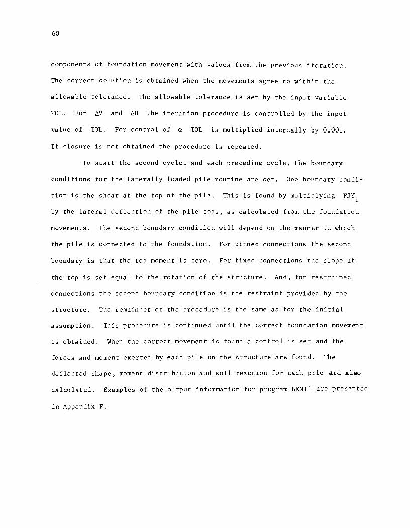
24. Foundation representation - Copano Bay.
25. Load deflection curve - Copano Bay
26. Soil Properties for generation of p-y curves - Copano Bay
27. Houston Ship Channel bent
28. Foundation representation - Ship Channel
29. Estimated axial load - deformation curve - Ship Channel
30. Soil properties for generation of p-y curves - Ship Channel
Page
64
. 64
67
69
70
71
71

Symbol
a
A
b
B
c
C
E
E s
F v
h
I
J x
J y
J m
K o
M
p
Typical Units
in
in
lb
lb
in
. 4 1n
lb/in
lb/in
in-lb/in
in-lb
in-lb
lb
NOMENCLATURE
Definition
Horizontal distance to pile top
Recursive coefficeint
Vertical distance to pile top
Recursive coefficient
Cohesion .
Recursive coefficient
Modulus of elasticity (Pile)
Soil modulus
Horizontal load on pile
Vertical load on pile
Increment length
Pile moment of inertia
Axial secant modulus
Lateral secant modulus
Moment secant modulus
Coefficient of active earth pressure
Coefficient of passive earth pressure
Moment
Moment on pile top
Soil reaction
Vertical load on foundation
xv

xvi
Symbol Typica 1 Units Definition
PH lb Horizontal load on foundation
R lb- in2 Pile s ti ffness (E1)
V lb Shear
w in Pile diameter or pile width
x t
in Axial movement of pile top
X in Distance from soil surface
y in Lateral pile deflection
Q' rad Rotation of founda tion
y lb/in3 Soil uni t weigh t
llH in Horizontal foundation movement
rw in Vertical foundation movement
€ in/in Strain
'3 rad Pile batter
CJ Ib/in 2 Stress
all lb/in2 Deviator s tres s (01
- (3
)
-:b degrees Angle of internal friction

CHAPTER I
INTRODUCTION
The purpose of this study is to review and expand upon existing
methods for analyzing foundations which are supported on pile groups consist
ing of vertical and batter piles. The expansions of the existing methods are
aimed at solutions for problems of bridge bents supported on piling. It is
believed that the resulting method will apply equally well to other types of
piling supported foundations, if the cap connecting the piles is rigid in
relation to the flexibility of the pile.
When a grouping of vertical piles is subjected to horizontal loading,
the stiffness of the piles may result in a portion of the horizontal load
being transferred to the lower soil strata. A larger portion of the horizontal
load will be transferred directly to the upper soil layers as the piles bend
laterally. If the upper soil layers are weak and highly compressible, the
lateral deflection which occurs may be excessive.
By using batter piles in a pile grouping, the portion of the horizontal
load transferred to the upper soil layers is reduced, since the component of
the horizontal force parallel to the axis of the batter pile is transferred to
the lower strata through axial loading. This transfer of horizontal load
into axial load in batter piles will usually reduce the deflection of the pile
group, since piles are stiffer under axial loading than under bending type
loading and the lower soil strata are usually stiffer than the upper soil
strata.
It is desirable to know the forces on each pile and the load deflection
behavior of each pile in order to make a more complete appraisal of the ade
quacy of a pile-supported foundation. When only vertical piles are used and
I
2
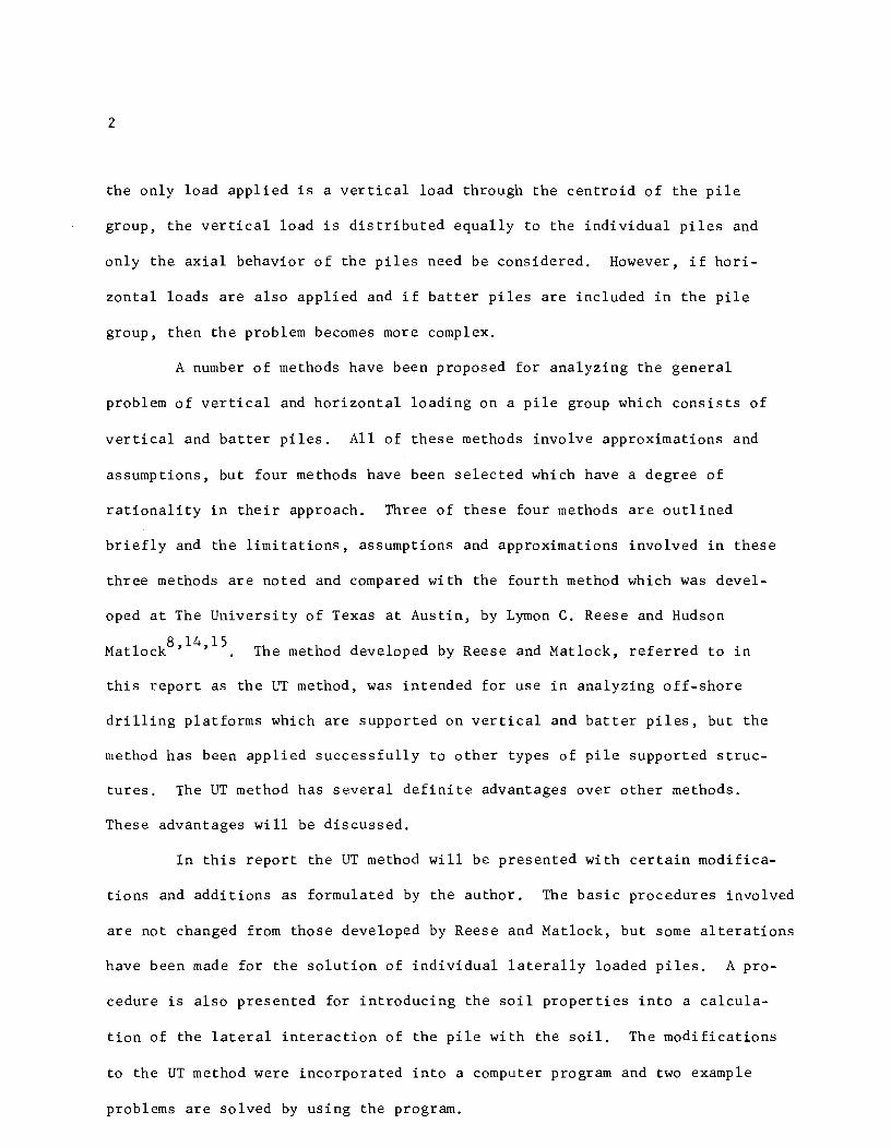
the only load applied is a vertical load through the centroid of the pile
group, the vertical load is distributed equally to the individual piles and
only the axial behavior of the piles need be considered. However, if hori-
zontal loads are also applied and if batter piles are included in the pile
group, then the problem becomes more complex.
A number of methods have been proposed for analyzing the general
problem of vertical and horizontal loading on a pile group which consists of
vertical and batter piles. All of these methods involve approximations and
assumptions, but four methods have been selected which have a degree of
rationality in their approach. Three of these four methods are outlined
briefly and the limitations, assumptions and approximations involved in these
three methods are noted and compared with the fourth method which was devel-
oped at The University of Texas at Austin, by Lymon C. Reese and Hudson
M 1 k8,14,15
at oc . The method developed by Reese and Matlock, referred to in
this report as the UT method, was intended for use in analyzing off-shore
drilling platforms which are supported on vertical and batter piles, but the
method has been applied successfully to other types of pile supported struc-
tures. The UT method has several definite advantages over other methods.
These advantages will be discussed.
In this report the UT method will be presented with certain modifica-
tions and additions as formulated by the author. The basic procedures involved
are not changed from those developed by Reese and Matlock, but some alterations
have been made for the solution of individual laterally loaded piles. A pro-
cedure is also presented for introducing the soil properties into a calcula-
tion of the lateral interaction of the pile with the soil. The modifications
to the UT method were incorporated into a computer program and two example
problems are solved by using the program.

CHAPTER II
METHODS OF ANALYSIS OF BATTER PILE FOUNDATIONS
GENERAL CONSIDERATION OF PROBLEM
A procedure is available for design of pile supported foundations in
which all the piles are vertical and in which the applied loads may be resolved
into a vertical force through the centroid of the pile group. The procedure
involves two steps. First, the allowable be'aring capacities of the individual
piles are obtained by applying an appropriate safety factor to the ultimate
capacities of the piles as determined either from load tests, from driving
characteristics, or from other theoretical procedures. Second, the total
applied load is divided by the number of piles in the foundation to obtain
the load on each pile. If this load does not exceed the allowable bearing
capacities of the individual piles, then the design is considered adequate.
Terzaghi and Peck24
also recommended that the design be checked by computing
the allowable bearing capacity of the pile group against breaking into the
ground as a unit.
The above procedure for vertical piles and vertical loads gives no
indication of the deflections which occur for intermediate loads, but only
the allowable load which may be sustained with a safety factor against
excessive settlement of the foundation. The procedure must also be considered
as an approximation since it is felt that all piles do not carry the same load.
The load which is carried by a pile is influenced by the spacing of adjacent
piles but the exact relationship of this influence is not known. This in-
fluence is frequently estimated by empirical rules of thumb or approximations.
If the pile group includes batter as well as vertical piles and if
the group is subjected to horizontal and vertical loading, the analysis be-
comes more complicated. In a rigorous analysis the horizontal and moment
3
4
resistance offered by the piles must be considered, as well as the axial
resistance. b 19 d· f h d Ro ertson 1scusses some 0 t e assumptions an approximations
frequently employed to handle horizontal and moment resistance. Robertson
points out that some of these assumptions may misrepresent a batter pile
structure and that the methods of analysis which employ these assumptions may
have limited usefulness due to the inaccuracy of the approximations involved.
There is some degree of approximation in all methods which have been
proposed for the analysis of foundations supported by batter piles. Brief
discussions of the methods proposed by Carl Culmann, as reported by Terzaghi
24 25 7 and Peck ,C. P. Vetter and Alexander Hrennikoff will be presented in
the following sections. The discussions will include lists of the limitations
and approximations involved in each method. These methods are considered to
be representative of the available methods for analysis of foundations support-
ed on batter piles.
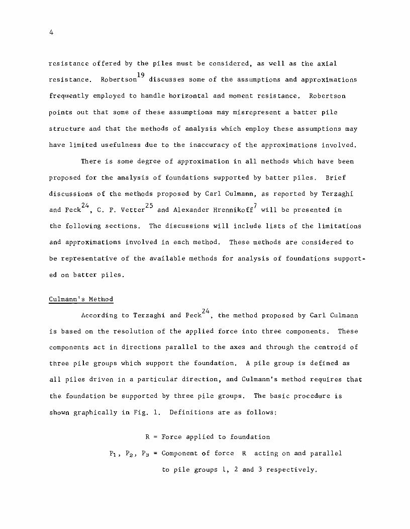
Culmann's Method
24 According to Terzaghi and Peck ,the method proposed by Carl Culmann
is based on the resolution of the applied force into three components. These
components act in directions parallel to the axes and through the centroid of
three pile groups which support the foundation. A pile group is defined as
all piles driven in a particular direction, and Culmann's method requires that
the foundation be supported by three pile groups. The basic procedure is
shown graphically in Fig. 1. Definitions are as follows:
R Force applied to foundation
Component of force R acting on and parallel
to pile groups 1, 2 and 3 respectively.

I I I I I I I I I
\ \ \ \ \ \ \ \ \ \
Group 3
~~\
PI
'----, ~ --I -- 1 ---- I -\ I
\ I \ I \ I \ I \ I \\ I
Group 2 Group I
Fig. 1. Graphical representation of Culmann's method.
5

6
The method is subject to the following limitations:
1. Solution is limited to two dimensional configurations.
2. The foundation must be supported by three nonparallel
groups of piles.
3. No load-displacement relationships are considered for the
foundation or the piles.
The assumptions and approximations involved are as follows:
1. The piles develop only-axial forces.
2. The foundation is statically determinate.
Vetter's Method
25 The method presented by C. P. Vetter is similar to the methods
developed earlier by Swedish engineers. Vetter mentions a number of earlier
works in the acknowledgments to his paper.
This method utilizes the concept of an elastic center (center of
rotation) about which the foundation rotates. Forces through the elastic
center cause only translation, without rotation, while a moment about the
elastic center will cause a rotation, without translation. This translation
and rotation of the foundation will cause movement of the pile heads. The
method proposed by Vetter consists of locating the elastic center of the
foundation, and determining the forces required to produce small elastic de-
formations in the piles. The applied loads are resolved into a force through
the elastic center, and a moment about the elastic center. By adjusting the
applied forces in relation to the forces required to produce elastic deforma-
tions in the piles, the forces on the piles due to the applied load may be
found.

7
Axial, lateral, and rotational resistances of the piles are consi-
dered. The forces developed will correspond to an axial deflection, a lateral
deflection and a rotation of the pile head. The lateral pile resistance
offered by the pile is simulated by assuming the pile fixed at some depth
"h" as shown in Fig. 2. The pile may be considered as pinned or fixed to
the structure, depending on the rotational resistance offered by the pile.
The effect of lateral and rotational resistance is simulated by intro
ducing imaginary "dummy" piles perpendicular to the real piles and considering
the real piles as columns, pinned to the footing and pinned at some depth in
the soil. The "dummy" piles are also considered as pinned columns.
By introducing "dummy" piles the lateral load-deformation character
istics are simulated by the axial behavior of the "dummy" piles. The location
and length of the "dummy" pi les will depend on the manner in which the pi Ie
is connected to the structure and the location of the point of fixity. The
cross-sectional area of the "dummy" pile is expressed in terms of the cross
sectional area and stiffness of the real pile. If the pile shown in Fig. 2
is considered fixed to the structure, the "dummy" pile representation is
shown in Fig. 3.
With the representation shown in Fig. 3, the resistance of the pile
is simulated by axial forces in the pin-connected columns. The magnitude of
the axial forces in the columns are determined by the force and moment through
and about the elastic center, and by the location of the pile head. From the
force in the pinned column representing the axial behavior of the real pile,
the axial pile movement may be predicted. However, no method is available for
predicting the lateral pile movement or the foundation movement.
Vetter's method is subject to the following limitations:
1. Solution is limited to two-dimensional configurations.

8
Connection May Be Pinned or Rigid
Fig. 2. Pile simulation for Vetter's method.
Fig. 3. Dummy pile representation for Vetter's method.
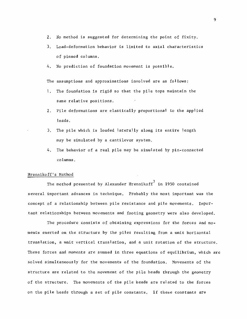
2. No method is suggested for determining the point of fixity.
3. Load-deformation behavior is limited to axial characteristics
of pinned columns.
4. No prediction of foundation movement is possible.
The assumptions and approximations involved are as follows:
1. The foundation is rigid so that the pile tops maintain the
same relative positions.
2. Pile deformations are elastically proportional to the applied
loads.
3. The pile which is loaded laterally along its entire length
may be simulated by a cantilever system.
4. The behavior of a real pile may be simulated by pin-connected
columns.
Hrennikoff's Method
9
The method presented by Alexander Hrennikoff7
in 1950 contained
several important advances in technique. Probably the most important was the
concept of a relationship between pile resistance and pile movements. Impor
tant relationships between movements and footing geometry were also developed.
The procedure consists of obtaining expressions for the forces and mo
ments exerted on the structure by the piles resulting from a unit horizontal
translation, a unit vertical translation, and a unit rotation of the structure.
These forces and moments are summed in three equations of equilibrium, which are
solved simultaneously for the movements of the foundation. Movements of the
structure are related to the movement of the pile heads through the geometry
of the structure. The movements of the pile heads are related to the forces
on the pile heads through a set of pile constants. If these constants are

10
known and the pile-head movements are known the pile forces and moments may
be found.
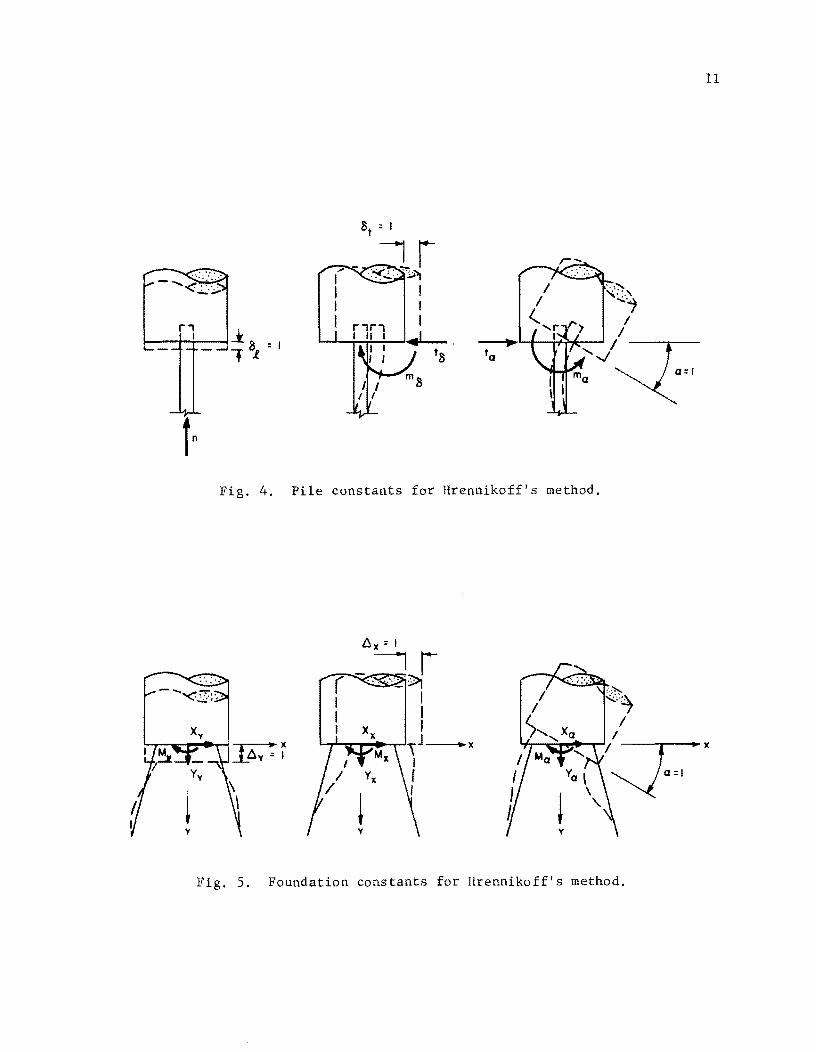
Hrennikoff defines the pile constants as the forces with which the
pile acts on the foundation when the pile head is given a unit displacement.
There are three sets of constants, corresponding to three different kinds of
displacements. The five pile constants (n, t 6 , m6
, ta
, mJ are shown in
Fig. 4 with the corresponding displacements (6 t , 6t , a).
5 By the Betti theorem t = m
a 6 leaving only four pile constants.
The pile constant n is evaluated using an approximate formula. The con-
stants and m are evaluated by considering the pile as a beam on a
an elastic foundation of infinite length, loaded at the free end. The elastic
modulus of the soil is evaluated using approximate formulas developed by the
author.
The pile constants, number of piles, and the geometry of the founda-
tion are combined to evaluate the foundation constants. The foundation con-
stants are defined as the resultant forces with which all piles act on the
footing, when the footing is given a unit translation in the positive direction
of one of the axes, or a unit rotation about the origin in a clockwise direc-
tion. The coordinate system and the foundation constants are shown in Fig. 5.
The constants X, Y, M, X, Y, M, X, Y and M are obtained x x x y y y a a a
by giving the foundation a displacement x = 1, Y = 1 or a = 1 as mentioned
previously.
By the Betti theorem Y = X x y'
M = X x a' and M = Y
Y a leaving only
six constants to be evaluated. The equations of equilibrium for the footing
are then
'--
11
Fig. 4. Pile constants for Hrennikoff's method.
;,~ ",,:.~
/ L.f.,...-c::;.~.......,~ I I::;::'
y
Fig. 5. Foundation constants for Hrennikoff's method.

12
X 6 + X 6 + X a + X 0 x x y y a
X 6 + Y 6 + Y a + Y 0 Y x Y y a
X 6 + Y 6 + M a + M 0 a x a y a
where X, Y, and M are the forces and moment applied to the footing
through and about the origin of the coordinate system. Once the structure
movements (6, 6 and a) are found the forces and moments exerted by the x y
piles may be found by working backwards. The movements of the pile head may
also be found.
Hrennikoff's method is subject to the following limitations:
1. Solution is limited to two-dimensional configurations.
2. All piles must behave alike with regard to the load-deformation
relation.
The approximations and assumptions involved are as follows:
1. Pile deformations are elastically proportional to the applied
loads.
2. The foundation is rigid so that the pile tops maintain the
same relative positions.
3. Foundation movements are small.
4. The piles are infinite in length.
COMPARISON OF METHODS WITH DT METHOD
Before beginning a detailed presentation of the DT method the basic
assumptions involved in the method will be presented and compared with assump-
tions in the three methods previously discussed. It is felt that the advan-
tages of the DT method will be apparent after this discussion.
13
Two Dimensional Configuration
The methods of Vetter, Culmann, and Hrennikoff are limited to the
analysis of two dimensional problems, This does not limit the solution to
foundations with piles in only one plane, It does, however, limit the solu-
tion to problems which have all piles parallel with, and symmetrical with
respect to a vertical plane of symmetry, Similarly the resultant of all
external forces and moments must be located in the plane of symmetry,
The UT method is also subject to the limitation of two dimensional
analysis, There are structures for which a three dimensional solution is
desirable, However, for many practical engineering problems a two dimensional
1 " ff" Th d' . 1 1 . 1,21 '1 bl b ana YS1S 1S su 1C1ent. ree 1menS10na so ut10ns are ava1 a e ut
will not be considered in this study,
Rigidity of the Foundation
Culmann's method, since it considers only equilibrium of the founda-
tion, requires no assumptions concerning the rigidity of the foundation, For
Vetter's and Hrennikoff's methods, as well as the UT method, the pile cap is
assumed to be rigid so that the pile heads maintain the same relative positions
before and after movement.
Connection of Piles to the Foundation
No consideration is given to the method of connecting the piles to the
foundation in Culmann's method since the analysis is based on each pile group
exerting a resultant force parallel to the piles in that group, For the
methods of Vetter and Hrennikoff the piles may be fixed or pinned to the
structure, For the UT method the piles may be fixed, pinned or attached in
such a manner that the foundation exerts some constant rotational restraint
14
on the pile. That is, the moment on the top of the pile divided by the
slope at the top of the pile will be a constant.
Pile-Soil Interaction
For Cu1mann's method no pile-soil interaction is considered. Vetter's
method simulates the axial interaction by considering the pile as a column.
The lateral interaction is simulated by considering the pile as a beam with
a fixed end.
The axial interaction, for Hrennikoff's method, is characterized by
a constant. This constant is obtained by considering the axial compression
for the pile as if it were a free standing column. The lateral interaction
is characterized by a set of three constants obtained by considering the
pile as a beam of infinite length on an elastic foundation.
For the UT method the axial pile-soil interaction is obtained from
a load-deformation curve. No specific pile-soil interaction is specified,
but the overall axial behavior is specified by the load-deformation curve.
The lateral interaction is specified by a set of deflection-reaction curves.
These curves, referred to as p-y curves, establish the relationship between
the deflection of the pile and the reaction exerted by the soil. These curves
are nonlinear as opposed to the linear behavior for the methods of Vetter and
Hrennikoff. The procedure for obtaining p-y curves and the manner in which
they are used in the analysis will be discussed later, but the point to be
emphasized here is that in the UT method the soil-pile interaction is non
linear as compared to the linear behavior which is assumed for the other
methods of analysis.
Soils do not deflect linearly under load. This can be seen by noting
the nonlinear shape of the stress-strain curves for soils as obtained from

15
triaxial test. This would indicate that a consideration of a nonlinear inter
action will yield more realistic results.
Load - Movement Relationships
Since Culmann's approach is based only on equations of equilibrium,
no prediction of the movements resulting from the applied loads is possible.
Similarly, Vetter's method provides no means for predicting foundation move
ment.
With Hrennikoff's method the foundation movement is defined by a hori
zontal and vertical translation and a rotation. These movements are related
to the forces on the foundation by a set of foundation constants. The rela
tionship between applied load and foundation movement is linear since they
are related through a set of constants. Similarly the force-deflection rela
tionship between pile-head movement and applied force is linear since they
are related by the pile constants.
For the DT method the movement of the foundation is defined by two
translations in the direction of the established coordinate system, and a
rotation about the origin of the coordinate system. The loads on the founda
tion are resolved into two forces through the origin of the coordinate system
and a moment about the origin. The movements of the pile heads are related
to the foundation movement by the geometry of the system. The forces on the
pile heads are related to the pile-head movements by nonlinear factors. All
of these relations are combined into three equations of equilibrium for the
foundation. From these equations the three movements of the structure are
obtained. Since the relationships between pile-head deflection and pile
reaction are nonlinear, an iterative process is necessary for establishing
an equilibrium position for the structure. Once the equilibrium position is
found, the deflection of the pile head and reactions may be obtained.

16
CONCLUSIONS
The UT method and Hrennikoff's method offer several major advantages
over the methods of Culmann and Vetter. The method of Culmann was the first
method proposed and it is limited by its failure to consider deflection of
the foundation system. Vetter's method was the next method proposed and it
introduces several improvements, but it is still limited by several assump
tions.
The method of Hrennikoff and the UT method are similar in their
approach. However, the UT method introduces two major improvements. Probably
the most important of these is the use of nonlinear pile-soil resistance rela
tionships. The second major improvement of the UT method is that it permits
the rotational stiffness of the structure or pile-head restraint to be in
cluded in the analysis.

PURPOSE
CHAPTER III
THEORETICAL DEVELOPMENT
In the following sections the theory involved for the UT method will
be developed. In the first section the coordinate systems and sign conven
tions for movements and forces will be established. In the second section
the relationships between foundation movement and pile-head movements will
be developed. Relations between foundation forces and pile reactions are
established in section three. In the fourth section relations between pi1e
head movement and pile reaction will be developed. In the final section the
equilibrium equations will be established.
COORDINATE SYSTEMS AND SIGN CONVENTIONS
Two types of coordinate systems are established. Examples are illus
trated in Fig. 6. A horizontal axis "a" and a vertical axis "b" are estab
lished relative to the foundation. Foundation movements, forces and dimen
sions are related to these axes. The location of this system is completely
arbitrary, but proper location will simplify calculations for most founda
tions.
For each pile an x-y coordinate system is established. The "x"
axis is parallel to the pile and the "y" axis is perpendicular to the pile.
Subscripts are used to indicate the particular pile. Pile deflection and
forces are related to these systems.
The coordinates of the pile heads as related to the a-b axes are
shown in Fig. 6. In the example all coordinates are positive. The batter of
17

18
b
~--- 01(+) ----...-.I
.... ------- 0 2 1+1
b
Fig. 6. Geometry of foundation.
t / / / / /
M1+1 /
/ P H1+1 PVI+1 /
Fig. 7. Sign convention for foundation forces and movements.
o
o

19
the piles is positive counter clockwise from the vertical and negative clock
wise from the vertical as shown.
The external loads on the foundation are resolved into a vertical
and horizontal component through the origin of the structural coordinate
system and a moment about the origin. The sign convention established is
illustrated in Fig. 7.
The external loads M, PV
' and PH will cause the foundation to
move. If the a-b coordinate system is considered to be rigidly attached to
the foundation, the movement of the foundation may be related to the movement
of the coordinate system. These movements (6V, 6H, and ~) are shown in
Fig. 7 with positive signs.
Due to the movement of the foundation, forces will be exerted on the
foundation by the piles. The sign convention for these forces is illustrated
in Fig. S.
The sign conventions illustrated by Fig. Sa are consistent with those
previously established for the structure. The conventions illustrated by
Fig. Sb are consistent with those established in the solution of laterally
loaded pi1esS The differences should be carefully noted. The inconsistencies
are taken care of when the relations between foundation forces and pile forces
are developed.
The sign conventions for movements of the pile head are consistent
with the x-y coordinate system. A movement in the positive II x" direction,
which constitutes an axial compression, is considered as a positive movement.
A movement in the positive "y" direction is considered as a positive move-
ment. A rotation of the pile head will cause a change in the slope at the top
of the pile. The sign convention for slope is consistent with the usual

20
p. Sin S
P, SinS
a, Forces and moment structure sign convention,
b. Forces and moment pile sign convention,
Fig. 8. Forces and moment on pile head.
Fig. 9. Pile head movements x-y coordinate system.

manner in which slope is defined. The movements of the pile head are illus
trated in Fig. 9.
RELATIONS BETWEEN FOUNDATION MOVEMENTS AND PILE-HEAD MOVEMENTS
21
When the structure moves the pile heads move. Two assumptions are
made in order to relate structure movement to pile-head movement. The first
assumption is that the foundation is rigid so that the pile heads maintain
the same relative positions before and after'movement. The second assumption
is that the foundation movements are small. Because of this assumption the
approximation
et R::: tan et (1)
is valid.
In Fig. lOa diagrams are given of the lineal movements at the pile
head of a given pile in terms of the structural movements. The movement of
the structure is defined by the shift of the a-b axes to the position indi
cated by the a'-b ' axes. The pile head movement is from point Q to point
Q/. The total movement of the pile head is resolved into a component parallel
to the "a" axis (Llli + bet) and a component parallel to the "b" axis
(IN + aet).
Figure lOb illustrates the resolution of the horizontal and vertical
components of movement into components parallel and perpendicular to the direc
tion of the pile. These movements are designated as xt
and Yt. Considering
Fig. lOb the axial component of pile head movement may be written as
(lili + bet) sin e + (IN + aet) cos e (2)
and the corresponding lateral movement as

22
b
fbI I I I J J , J I J , , I
a
Pile Head
b
,--- --, \ VPile
I I I ,
O~-'r---~--~~--------------------~----41----~
~v '0.:..__________ :' r . 6H ---___ I
--/----
a. Lineal movements of pile head.
b. Resolution of movement into components.
I -- ----""'0'
J I I I I I I
Fig. 10. Movements of pile head - structural coordinate system.

23
(6H + ba) cos e - (6V + aa) sin e (3)
In addition to the lineal displacements of the pile head, the change
in slope of a tangent to the elastic curve will be considered. The change in
the slope will depend on the manner in which the pile is attached to the
foundation. If the pile is fixed to the structure, then the change in slope
will be equal to the rotation of the foundation. For the restrained case the
change in slope will depend on the moment applied to the pile top. For a
pinned connection the slope will depend on the deflected shape of the pile.
RELATIONS BETWEEN FOUNDATION FORCES AND PILE REACTIONS
The forces acting on the foundation and pile are illustrated, along
with sign convention, in Fig. 8. It has been noted that inconsistencies in
the sign conventions are present. These will be taken care of in the rela-
tions between the forces.
Considering Fig. 8 the relationship between moments on the structure
and moment on the pile may be written as
M s -M
t (4)
The relations between forces are obtained by resolving the forces on the pile
into components in the horizontal and vertical directions. With the sign con-
ventions considered, the components are summed as follows:
F v
Pt
sin e - Px
cos e
-P sin e - P cos e x t
(5)
(6)

24
PILE-HEAD MOVEMENT AND PILE REACTION
In the preceding sections the movement of the pile head and the forces
acting on the pile head have been defined. In this section relations between
pile reaction and movement will be developed.
For computational purposes the pile shown in Fig. lla may be simulated
by the set of springs as shown in Fig. llb. The springs will produce a force
parallel to the pile axis, P , x
and a force acting perpendicular to the pile
axis, Pt' The rotational spring will produce a moment about the pile top,
The forces produced by the springs will depend on the deflection of
the springs. Since the springs are nonlinear the movement and reaction are
not related by a single constant. It is assumed that curves can be obtained
which show spring reaction as a function of deflection. In Fig. 12 a hypo-
thetical set of load-deflection curves are drawn for a set of springs. If
the curves are single valued then the spring reactions may be calculated for
a particular deflection by
p : J x (7) x x t
Pt = J Yt (8) y
M ~ J Yt (9) t m
where J , J y' and J are the secant modulus values as illustrated in x m
Fig. 12.
It should be noted that the moment produced by the rotational spring
is proportional to the lateral deflection, rather than the rotation. For a
rotational spring this procedure is inconsistent with usual concepts. This

25
a. Pile and foundation. b. Springs and foundation.
Fig. 11. Spring representation of pile.
P, J, P, I Y t
Y,
J",= -M, I Y,
Yt
Fig. 12. Hypothetical spring load-deflection curves.
26
concept is used because it provides a convenient means for deriving and
solving the equilibrium equation for the structure.
The curves shown in Fig. 12 do not adequately explain the behavior of
a pile. It is not necessary that the exact nature of the curves be known.
The representation shown is only for the formulation of the equilibrium
equations. The procedure for calculating values for J , x J , y
and J will m
be discussed in the following chapters. However, for the formulation of the
equilibrium equations, Eqs. 7, 8, and 9 are sufficient, since they will be
applicable no matter what kind of relationship exists between the loads and
the displacements.
EQUILIBRIUM EQUATIONS
The relations between forces and movements for the structure and the
pile have been developed in the preceding sections. In this section, these
relations will be combined to form three equations of equilibrium for the
structure. The form of the equations is such that an iterative type solution
may be used. This is necessary since the system is nonlinear.
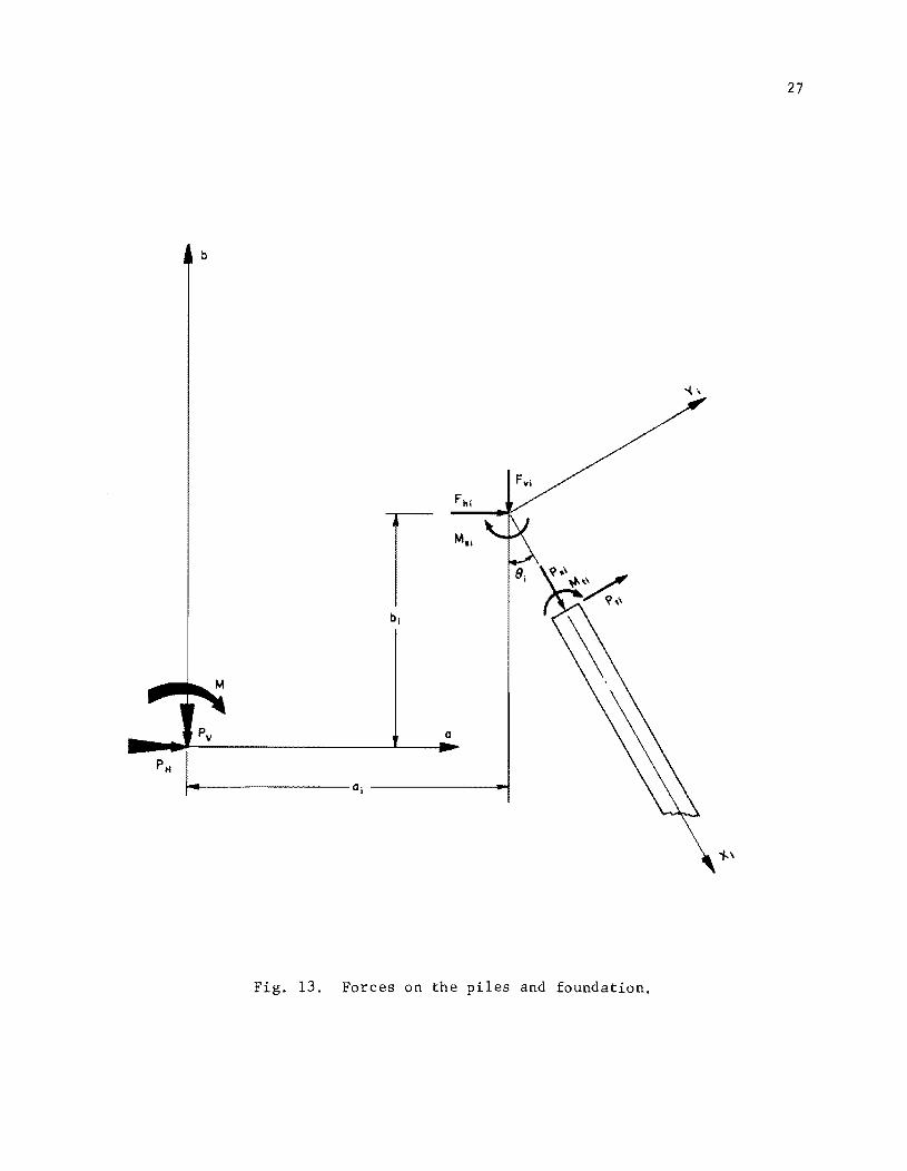
Consider a foundation supported by n piles. The coordinate system
and the ith pile are shown in Fig. 13. The external loads applied to the
foundation are resolved into the forces and moment through and about the origin
of the coordinates as shown in Fig. 13. The forces and moment exerted by each
pile are shown as F ., V1
and M . S1
in Fig. 13. The three equations are
obtained by summing forces in the horizontal and vertical directions and by
summing moments about the origin of the a-b coordinate system. Performing
these operations the equilibrium equations may be written as
27
b
Fig. 13. Forces on the piles and foundation.
28
n L: F . + Pv 0 i=l V~
(10)
(11)
n L: (M. + a. F . + b. F
h.) + M = 0 •
i=l s~ ~ V~ ~ • (12)
Substituting Eqs. 4, 5, and 6 into Eqs. 10, 11, and 12 and rearranging
n Pv L: (P . cos e. - P
ti sin e. )
i=l x~ ~ ~ (13)
n P = L: (P . cos e. + P
xi sin e.)
H . 1 t~ ~ ~ ~=
(14)
n
[Mti + M = L: a. (P . cos e. - P ti sin e.) + i=l
~ x~ ~ ~
b. (P t' cos e. + P xi sin ei8 ~ ~ ~
(15)
Substituting Eqs. 7, 8, and 9 into Eqs. 13, 14, and 15 the equilibrium
equations may be written as
n L: (J . x . cos e. i=l x~ t~ ~
n
PH = L: (J . Yt . cos e.; + JXi
x t .; sin e.) i=l Y~ ~ • •• ~
(16)
(17)

n [-M ~ J Yti + a. (J . x cos e. - J .... Yti sin e. ) i=l
mi 1 X1 ti 1 yl. 1
+ b. (J Y ti cos e. + J x sin ei ) ] (18) 1 yi 1 xi ti •
The equations are modified further by substituting Eqs. 2 and 3 into Eqs. 16,
17, and 18 and rearranging to obtain
M
~ {rJ .cos2
e.+J .sin2e.]
i=l LX1 1 y1 1 tN + [(J .-J .)Sine.cose.] X1 y1 1 1
+ ra.(J .cos 2 e.+J .sin2
e.)+b.(J .-J .)Sine.cose.] a} l1 X1 1 y1 1 1 X1 y1 1 1
(19)
~ {[(J .-J .)(Sine.cose.)] i=l X1 y1 1 1
+ [a.(J .-J .)sine.cose.+b.(J .cos2
e.+J .Sin2
e.)] 0 (20) 1 X1 y1 1 1 1 y1 1 X1 1
n L: i=l
sin e. + 1
a. (J . 1 X1
2 cos e. + J . 1 y1
. 2 S1n e. ) 1
+ b. (J . - J .) sin e. cos e.] 1 X1 y1 1 1 ~v + [-J . cos e. m1 1
+ a.(J .-J .)sine.cose.+b.(J .cos2 e.+J .sin2 e.)] t.H 1 X1 y1 1 1 1 y1 1 X1 1
+ [ J . m1 ( e) 2 2 2 a.sine.-b.cos . + a.(J .cos e.+J .sin e.)
1 1 1 1 1 X1 1 y1 1
29

30
+b~(J .COS 2 e.+J .sin2 e.)+2(J .-J .)(Sine.cose.)a.b.] O'}. (21) 1 y1 1 X1 1 X1 y1 1 1 1 1
Equations 19, 20, and 21 constitute the complete set of equilibrium
equations for a foundation. The loads on the foundation, the distance to the
pile tops, and the batter of the piles are known quantities. If the spring
modulus values are known, the three equations may be solved simultaneously
for eN, MI, and 0'. But, since the system is nonlinear, J , m
J , x and J Y
will not be constants. Because of this an iterative solution is required.
Chapter IV will present methods for handling the behavior of the individual
piles. Chapter V will give a brief summary of the iterative procedure used
in the computer program for solving the equilibrium equations.

CHAPTER IV
BEHAVIOR OF INDIVIDUAL PILES
In the preceding chapter equilibrium equations were developed for a
pile supported foundation. These equilibrium equations contain secant modulus
values obtained from the nonlinear load-deformation curves for individual
piles. This chapter deals with the methods used for obtaining the secant
modulus values for the individual piles.
The modulus J is obtained from the axial behavior of the pile. x
Modulus values J and J are obtained from the lateral behavior of the m y
pile.
AXIAL BEHAVIOR
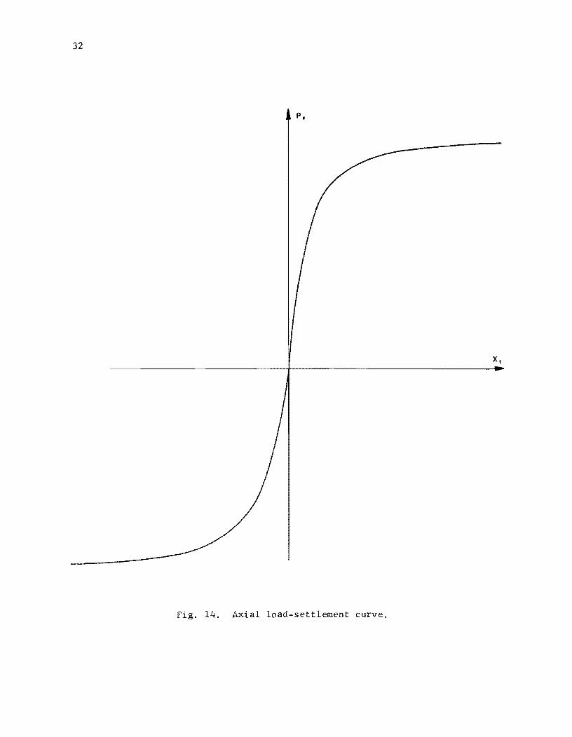
In order that a value for J be calculated, an axial load-deflection x
relation is necessary. The procedure employed involves finding a load-sett1e-
ment curve for the pile. A typical load-settlement curve is shown in Fig. 14.
The curve shown consists of two branches, corresponding to bearing and pullout
of the pile.
If a load-settlement curve is available, a value of secant modulus may
be obtained for any value of axial deflection by applying Eq. 7. This is a
simple procedure for obtaining J x
after the correct value for axial def1ec-
tion is found. The problem which arises is to find a load-settlement curve
which will accurately describe the axial behavior of a pile. Earlier methods
of analysis did not require that an exact load-settlement curve be found. A
computed ultimate axial load, or an ultimate load obtained from a full scale
load test was usually considered adequate for design purposes. For the pro-
posed method, a relationship between load and deflection is necessary. The
31
32
Fig. 14. Axial load-settlement curve.

33
axial behavior of piles is usually determined by one of three methods. These
are as follows:
1. Dynamic formulas
2. Static formulas
3. Full scale loading test.
Dynamic Formulas
Dynamic formulas such as that of Hiley as described by Chellis2
give
only a maximum pile capacity with no regard to corresponding movements. It
has been demonstrated that the dynamic formulas give very erratic results with
3 13 poor correlation between calculated and measured values of pile capacity ,
The various formulas have limited usefulness for the method considered because
of the lack of load-settlement data.
Static Formulas
The static formulas relate the load carrying capacity of the pile to
the soil properties. The usual procedure is to calculate a tip load using
11 12 some bearing capacity formula, such as that suggested by Meyerhof ' ,and
some shaft load which is transferred to the soil through skin friction along
the pile. Accurate prediction of skin friction is difficult but suggested
values are available2
. The bearing capacity and shaft load are added to ob-
tain the total pile capacity. This method is also limited by the lack of
load-settlement data. If the dynamic and static formulas are to be of any
value to the analysis under consideration, some method must be found to relate
load to deflection.
16 The method proposed by Reese seems to offer a great deal of promise
for predicting load-settlement curves from soil data. 4 Coyle has compared
measured values with values calculated using this method, for steel friction

34
piles in clay. The correlation obtained was quite good. However, the use-
fulness of this method is limited by the lack of correlation for a range of
pile and soil types.
Full Scale Loading Test
The use of loading tests is the most reliable method presently avail-
able for predicting load-settlement curves. A pullout test and a bearing test
will give the desired load-deflection relation.
Conclusions
Of the methods discussed, the loading test gives results which best
represent the axial behavior of a pile. 16
The method suggested by Reese
will give reliable results provided the load transfer can be accurately pre-
dicted. The static and dynamic formulas have limited usefulness because of
the lack of load-deflection information. A load-deflection curve may be ob-
tained by assuming some relation between load and deflection based on the
calculated ultimate load. The accuracy of this procedure will depend on the
accuracy of the assumption, and it will probably give only a rough estimate.
LATERAL BEHAVIOR
For the calculation of the modulus value J a relationship between y
the shear at the top of the pile and the lateral deflection of the pile top
must be known. For the calculation of J some relationship between moment m
at the top of the pile and top deflection must be known. In the preceding
section, on the calculation of J , x
a load-deflection curve was used. This
is possible since it is assumed that the axial behavior of the pile is un-
affected by any lateral effects. That is to say that the axial load on the
pile is dependent only on the axial deflection of the pile. A similar

assumption concerning lateral behavior is not true. Simple single-valued
curves for Pt
vs. and M vs. t
as shown in Fig. 12 do not exist
for a pile which is attached to a foundation.
35
Since a single-valued load-deflection relationship cannot be found, a
different approach must be taken for calculating J m and J . x
The approach
taken involves the solution for the deflected shape of the pile using finite
difference equations. Once the deflected shape is known the shear and moments
can be calculated and modulus values may then be calculated using Eqs. 8 and 9.
The interaction is nonlinear so that an iterative process must be employed to
find the correct modulus values. The iterative procedure will be explained
in detail in Chapter V. For the following discussion assume that the iterative
procedure is complete and that correct boundary conditions are applied to the
pile. With this in mind the finite difference solution for the laterally
loaded pile will be discussed and the calculation of the modulus value ex-
plained. The soil criteria used to determine the lateral interaction will
also be explained.
Finite Difference Solution for Laterally Loaded Piles
The finite difference approach to the solution of laterally loaded
6 piles was first suggested by Gleser This idea was further extended by
9 17 Reese and Matlock' . The method presented here is for the special case of
a laterally loaded pile and is similar to the method presented in Refs. 9
and 17, the differences being in the application of boundary conditions and
the addition of the effects of axial load on the lateral deflection.
The differential equations are derived by considering an element of
the pile as shown in Fig. 15. The sign of all forces, deflections, and slopes
shown are positive. It should also be noted that the axial load is constant
over the length of the pile. For piles this assumption is not consistent

36
Vb
Vt
T dy
V
T X
p.
V
dx
X
Fig. 15. Generalized beam column element.

37
with observed behavior, since it is known that some of the applied axial load
is transferred to the soil by skin friction along the shaft. The validity of
this assumption is based on the fact that the errors introduced will be in-
significant. Considering the problem from a physical standpoint it is known
that for most cases the skin friction increases with depth. This, plus the
fact that any lateral movement will cause a decrease in skin friction, leads
to the conclusion that the axial load removed by the skin friction in the
upper portion of the pile is small. Since the maximum moment occurs in the
top portion of the pile, and since it is the deflection of the pile top which
is of interest, the assumption of constant axial load will not significantly
affect the results of interest.
The reason for having the assumption of axial load constant on
the top of the pile is one of convenience. The addition of a variable axial
load could have been handled analytically but the effort required for obtain-
ing a solution would not be warranted because of uncertainties involved in
obtaining the nature of the variation.
Referring to Fig. 15 the equilibrium equations for the element may be
written as
and
where
dM V+P ~ dx - x dx
dV dx = - P
M = Bending moment
E Y s
o
x Distance along pile
(22)
(23)

38
V Shear
P Axial load (constant) x
y Lateral deflection
p = Soil reaction per unit length
E Soil modulus. s
By combining Eqs. 22 and 23 and differentiating, the following equation is
obtained:
d2 v Y + P ~
X dx2 o
The equation for shear is written as
v dM + P ~ dx x dx
and the equation for moment is written as
M
where
E Modulus of elasticity of the pile
I Moment of inertia of pile section
R EI (flexural rigidity).
(24)
(25)
(26)
Equations 24, 25, and 26 may be written in finite difference form
using the central-difference approximations. The equations will be written
for a general point referred to as station "i". Station numbering increases
from top to bottom of piles. The equations obtained for station "i" are as
follows:

where
+ R. 1 - 2P h2
+ E .h4) + y. 1(-2R. - 2R. 1 + P h2
) 1- X S1 1- 1 1- X
+ y. 2 (R. 1) = 0 1- 1-
(27)
- R. 1) + y. 1(2R. 1 - P h2
) + y. 2(-R. l)J (28) 1- 1- 1- X 1- 1-
h = Increment length.
2y. 1
(29)
The finite difference equations are used to obtain the deflected
39
shape of the pile. Once the deflected shape is obtained any other information
about the pile may be obtained by the application of the appropriate equations.
The pile is divided into "n" increments of length "h" as shown
in Fig. 16. In addition, two fictitious increments are added to the top and
bottom of the pile. The four fictitious stations are added for formulating
the set of equations but they will not appear in the final set of equations.
The coordinate system and numbering system used is illustrated in Fig. 16.
The procedure used is to write Eqs. 27, 28, and 29 about station
n+3. This results in 3 equations involving 5 unknown deflections (Yn+5'
Yn+4' Yn+3' Yn+2' Yn+1)' Two boundary conditions, Vn+3 = 0 and
Mn+3 = 0, are applied at station n+3. The deflections for the fictitious
stations n+4 and n+5 are eliminated from the three equations and the

40
r---, I I I I I I I I
2 ~----~ I I I I I I I I I I
3 r--- --"" -y
4
5
6 ~
n
n""
I I I I I I I I I I
n+4 ~--~-~ I I I I
n+5
I I I I
I L __ --....I
x
Fig. 16. Finite difference representation of pile.
41
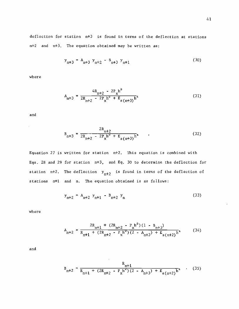
deflection for station n+3 is found in terms of the deflection at stations
n+2 and n+3. The equation obtained may be written as:
(30)
where
(31)
and
(32)
Equation 27 is written for station n+2. This equation is combined with
Eqs. 28 and 29 for station n+3, and Eq. 30 to determine the deflection for
station n+2. The deflection Yn+2 is found in terms of the deflection of
stations n+1 and n. The equation obtained is as follows:
A Y - B Y n+2 n+1 n+2 n (33)
where
(34)
and
(35)

42
The deflection for station n+l may be found in a similar manner. From
station n+l to the top of the pile the expressions for the deflection have
the same form. The general form of the equation is as follows:
where
and
A. ~
B. ~
(36)
2Ri _ l + Ri (2-2Bi + l ) + Ri + l (Ai + 2 Bi + l - 2B i + l ) - Pxh2
(1-Bi+ l )
c.
R. 1 ~-
C. ~
~
(37)
(38)
(39)
With the general expression the deflection of each station may be
expressed as a function of the deflection of the two stations immediately
above it. If the deflections for stations 3, 4, and 5 are written a set of
three equations involving five unknown deflections will be obtained. If two
boundary conditions are introduced the deflections for the fictitious stations
may be eliminated and the equations solved for the deflections. Once the de-
flections for stations 3 and 4 are found the deflections for the remainder of
the pile may be obtained by back substitution into the equations obtained for
the deflection of a station in terms of the deflection of the two stations
directly above it.

43
The expressions obtained for Y3 and Y4 will depend on the boundary
conditions applied to the top of the pile. Three sets of boundary conditions
are used resulting in three sets of equations.
For the first case the following boundary conditions are applied:
(40)
(41)
where Mt
and Pt
are the moment and lateral load applied to the top of the
pile. The application of these boundary conditions results in the following
expressions for Y3 and Y4:
where
Yo =f [R. (2 Ao B. - 4 B.) + Ro (2 - 2 B.) + 2Pxh2
BJ
+ Do Gj/f' [ Ro (2 B. - 2) + R. (4 B. - 2 Ao B.)
- 2 P x h 2
B 4J + G2 [R3 (4 - 2 ~) + R4 (2 A4 As
- 2 B5 - 4 A. + 2) + Pxh2 (- 2 + 2 A.) + Esoh~} (42)
Y4 Y3 ( A. - Baa G) ) B~ 11.:!
G2 (43)
M h2
D2 t R3
(44)
D3 2P h3
t (45)
G1 = 2 - ~ (46)
44
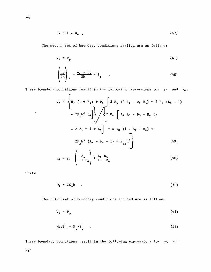
The second set of boundary conditions applied are as follows:
Vs = P t
Yi - Ya 2h
(47)
(41)
(48)
These boundary conditions result in the following expressions for Ya and Y4:
where
Ya fa (1 + B,) + D, [2 R, (2 B, - ... B,) + 2 Ra (B, - 1)
- 2P xh2
B']} It R, [ ~ ... - B, - B, B,
Y4 = Y3
D4 = 28 h t
+ 4 Ra (1 - ~ + B4 ) +
-1) + E h} S3
The third set of boundary conditions applied are as follows:
(49)
(50)
(51)
(41)
(52)
These boundary conditions result in the following expressions for Y3 and
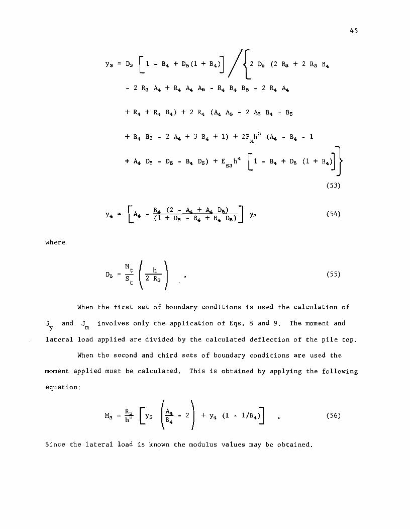
where
Y. = D3 [1 - B, + D5 (1 + B,)] / {2 D,; (2 .. + 2 .. B,
- 2 R3 A4 + R4 ~ As - R4 B4 Bs - 2 R4 ~
+ B4 Bs - 2 ~ + 3 B4 + 1) + 2P h2 (~ - B4 - 1 x
+ Po,. D, - D5 - B, D5 ) + E S3 h' [1 -B, + D, (1 + B, 8 } (53)
(54)
(55)
When the first set of boundary conditions is used the calculation of
J and J involves only the application of Eqs. 8 and 9. The moment and y m
45
lateral load applied are divided by the calculated deflection of the pile top.
When the second and third sets of boundary conditions are used the
moment applied must be calculated. This is obtained by applying the following
equation:
(56)
Since the lateral load is known the modulus values may be obtained.

46
Lateral Soil-Pile Interaction
In the preceding section the effect of the soil on the pile was shown
as a distributed reaction p. The soil reaction p was defined as:
p E Y s (23)
where E is the soil modulus and y is the lateral deflection. The soil s
reaction resists the deflection of the pile. For the derivation of the finite
difference equations it was assumed that the soil modulus values were known.
Since the soil-pile interaction is usually nonlinear an iterative procedure
is required to find the correct values of E . s
The following discussion deals
with the development of the relationship between lateral pile movement and
soil reaction. In the final section of this chapter the soil criteria used
will be discussed.
A typical relation between p and y is shown in Fig. 17. The soil
modulus is defined by Eq. 23. From Fig. 17 it is seen that the soil modulus
is the slope of the secant drawn from the origin to any point along the curve.
Since p is defined as the distributed soil reaction with units of force per
unit of length along the pile the soil modulus E will have units of force s
per unit length squared. Since the p-y curve for most soils is nonlinear,
an iterative procedure will usually be required to find the correct soil
modulus, and the corresponding deflected shape.
The p-y curves will depend on the soil properties. For most cases
the properties of the soil in a profile is not constant with depth. The usual
case being that the strength of the soil increases with depth. A typical
variation of shear strength of soil with depth is shown in Fig. l8a. Since
the strength of the soil will affect the p-y curves obtained, a variation
similar to that illustrated in Fig. l8b might be expected. It should be

c:
".c
/ /
/ /
/ /
/
/
/ /
/
////r E, ~ ply
/
y, in.
Fig. 17. Typical p-y curve.
47

48
.t::. -0-eD o
Shear Strength
a. Variation of shear strength with depth.
p
y
p
y
b. Variation of p-y curves with depth.
Fig. 18. Variation of soil properties with depth.
49
pointed out that the shear strength is not the only parameter which will
affect the p-y curve, although it does have considerable influence. The
purpose of the variation shown in Fig. l8b is only to illustrate the variabi-
lity of the p-y relation.
For use in the equations for deflection a value of soil modulus is
required for each station. If a p-y curve is available at a station and
the deflection is known, then a value for soil modulus can be obtained. If
a p-y curve is not available for a particular station, then a soil modulus
value is obtained by linear interpolation between p-y curves above and
below the particular station. The E values obtained are used in the solus
tion for the deflections. The iterative process is continued until closure
is obtained for the deflections.
Soil Criteria
The soil criteria presented here for obtaining p-y curves is derived
from theoretical and empirical considerations. It is limited by the fact that
criteria is available only for clay and sand. No criteria is available for
soil which has cohesion and also some angle of internal friction. It must
also be used with reservation since sufficient correlation with measured values
is not available. Work of this nature has been done but it is still confi-
dential information. Once this information becomes available to the engineer-
ing profession it will be possible to obtain more realistic p-y curves,
than are obtainable from the theory presented.
It is assumed that the p-y curves can be divided into two segments.
The portion designated as O-A and the portion designated as A-B in Fig. 19.
The segment O-A represents the early part of the curve and the segment A-B
represents the ultimate part of the curve. Because of this division the
construction of p-y curves may be carried out in two steps. First the

50
'" ",'"
'" A / B PUll - - -- - -- --~"--------..,~-----------
Ultimate Port of Curve
Early Port of Curve
o ~------------------------------------------------------~ o y
Fig. 19. Construction of p-y curve.
o~----------------------------------------~
o
Fig. 20. Stress-strain curve.
51
ultimate soil resistance is calculated and then the shape of the early part
of the curve is obtained. The horizontal line representing the ultimate soil
resistance and the early part of the curve are then joined to form a continuous
curve. In the following sections the procedure will be explained for clay and
then sand.
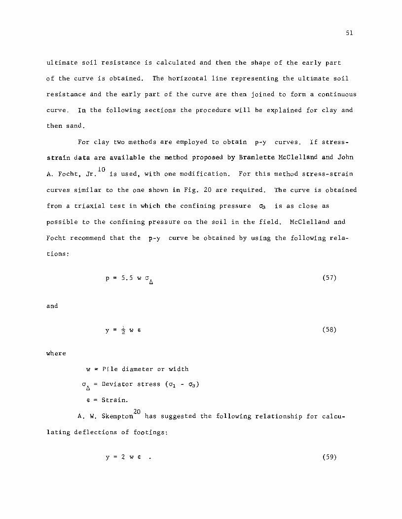
For clay two methods are employed to obtain p-y curves. If stress-
strain data are available the method proposed by Bramlette McClelland and John
10 A. Focht, Jr. is used, with one modification. For this method stress-strain
curves similar to the one shown in Fig. 20 are required. The curve is obtained
from a triaxial test in which the confining pressure 03 is as close as
possible to the confining pressure on the soil in the field. McClelland and
Focht recommend that the p-y curve be obtained by using the following rela-
tions:
p (57)
and
y 1 2 w € (58)
where
w = Pile diameter or width
€ = Strain.
20 A. W. Skempton has suggested the following relationship for calcu-
lating deflections of footings:
y 2 w € (59)

52
It is felt that the best value to use for deflection would be one between the
values calculated using Eqs. 58 and 59. The equation suggested is:
y W € • (60)
Using Eqs. 57 and 60 and the stress-strain curve a corresponding p-y curve
may be obtained.
It is assumed that the test is run until failure is obtained. That
is, the maximum value for a~ obtained will represent the ultimate value
which may be carried by the soil. Because of this, the value for p calcu-
lated using the ultimate value of is considered to be the ultimate soil
resistance.
If no stress-strain curves are available, but the shear strength and
unit weight are known, p-y curves can be obtained. Two expressions are
available for calculating the ultimate soil resistance for clay. These equa-
18 tions were suggested by Reese and are as follows:
and
where
y w X + 2 c w + 2.83 c X
11 cw
Y = Unit weight
w Pile diameter or width
X Depth from soil surface
c = q /2 = Cohesion. u
(61)
(62)
The smaller of the two values obtained from Eqs. 61 and 62 is used. Equation
61 will usually control near the surface since it is based on the occurrence
of a wedge type failure and Eq. 62 will control at depth since it is based
on the soil failing by flowing around the pile.
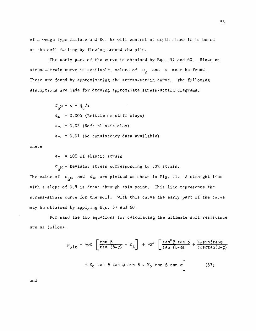
The early part of the curve is obtained by Eqs. 57 and 60. Since no
stress-strain curve is available, values of and € must be found.
These are found by approximating the stress-strain curve. The following
assumptions are made for drawing approximate stress-strain diagrams:
where
a 50 = C = q /2 /::. u
€so 0.005 (Brittle or stiff clays)
€~ 0.02 (Soft plastic clay)
€soO.Ol (No consistency data available)
€~ = 50% of elastic strain
a ~ = Deviator stress corresponding to 50% strain. /::.
53
The value of a /::.50 and €so are plotted as shown in Fig. 21. A straight line
with a slope of 0.5 is drawn through this point. This line represents the
stress-strain curve for the soil. With this curve the early part of the curve
may be obtained by applying Eqs. 57 and 60.
For sand the two equations for calculating the ultimate soil resistance
are as fo llows :
x [tan ~ _ K ] + y~ [tan2 Stan ct + KosinStan¢
Pult Yw tan (S-¢) A tan (S-¢) coscttan(S-¢)
+ Ko tan Stan ¢ sin S - Ko tan Stan ctJ (63)
and

54
bel CI' o
2
log €
Fig. 21. Approximate log-log plot of stress-strain curve.
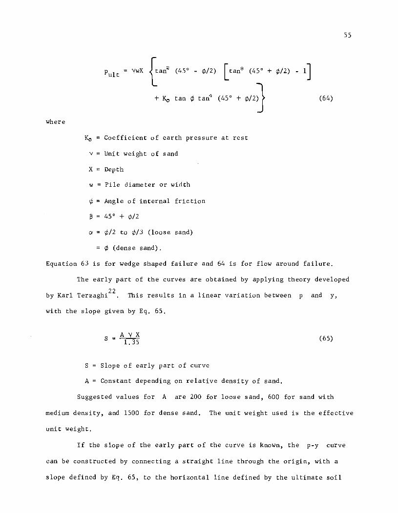
where
= ywX
+Ko
(45 0 - ¢/2) [tan8 (45 0 +
tan ¢ tan' (45 0 + ¢/2)
Ko = Coefficient of earth pressure at rest
y Unit weight of sand
x = Depth
w = Pile diameter or width
¢ = Angle of internal friction
~ = 45 0 + ¢/2
a ¢/2 to ¢/3 (loose sand)
¢ (dense sand),
(64)
Equation 63 is for wedge shaped failure and 64 is for flow around failure,
55
The early part of the curves are obtained by applying theory developed
b 1 h,22
y Kar Terzag 1 This results in a linear variation between p and y,
with the slope given by Eq. 65,
s A y X 1. 35
S = Slope of early part of curve
A = Constant depending on relative density of sand.
(65)
Suggested values for A are 200 for loose sand, 600 for sand with
medium density, and 1500 for dense sand. The unit weight used is the effective
uni t weight,
If the slope of the early part of the curve is known, the p-y curve
can be constructed by connecting a straight line through the origin, with a
slope defined by Eq. 65, to the horizontal line defined by the ultimate soil

56
resistance. This results in a p-y curve which consists of two straight
lines. When one considers the behavior of a sand it will be noted its be
havior is not linear. Because of this the p-y curve obtained should be
considered as an approximation.
Conclusions
In this chapter the behavior of a single isolated pile has been consi
dered. The axial and lateral behavior of the pile was considered and the
methods for calculating the spring modulus values explained. The soil criteria
used for obtaining p-y curves was also considered. Certain limitations of
the procedures used were discussed. Further limitations will be considered in
Chapter VII.
CHAPTER V
COMPUTATIONAL PROCEDURE
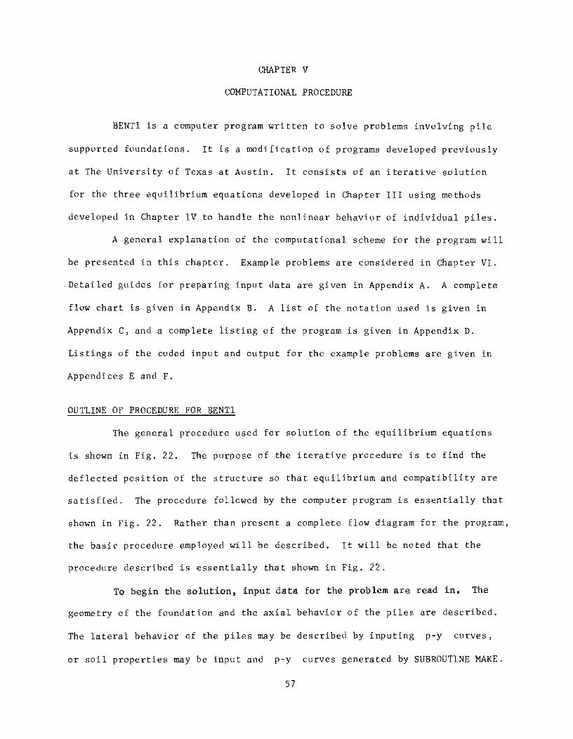
BENTI is a computer program written to solve problems involving pile
supported foundations. It is a modification of programs developed previously
at The University of Texas at Austin. It consists of an iterative solution
for the three equilibrium equations developed in Chapter III using methods
developed in Chapter IV to handle the nonlinear behavior of individual piles.
A general explanation of the computational scheme for the program will
be presented in this chapter. Example problems are considered in Chapter VI.
Detailed guides for preparing input data are given in Appendix A. A complete
flow chart is given in Appendix B. A list of the notation used is given in
Appendix C, and a complete listing of the program is given in Appendix D.
Lis of the coded input and output for the example problems are given in
Appendices E and F.
OUTLINE OF PROCEDURE FOR BENTI
The general procedure used for solution of the equilibrium equations
is shown in Fig. 22. The purpose of the iterative procedure is to find the
deflected position of the structure so that equilibrium and compatibility are
satisfied. The procedure followed by the computer program is essentially that
shown in Fig. 22. Rather than present a complete flow diagram for the program,
the basic procedure employed will be described. It will be noted that the
procedure described is essentially that shown in Fig. 22.
To begin the solution, input data for the problem are read in. The
geometry of the foundation and the axial behavior of the piles are described.
The lateral behavior of the piles may be described by inputing p-y curves,
or soil properties may be input and p-y curves generated by SUBROUTINE MAKE.
57

58
Set tN, llH and ex equal to zero.
Set the deflection of each pile top (x ., y .) equal to 1. 0; t~
Set initial boundary conditions for use in laterally loaded pile solution.
Calculate FJX. using ~ x . and load settle-
t~ f"l ment curve or p~ e.
Calculate FJY. and FJM. using laterally loa~ed pile solution with appropda te boundary conditions.
Calculate 6V, llH, and ex by simul taneous solution of three equilibrium equations.
Compare calculated 6.V, till, and ex values with previous values.
Closure obtained. Make final calculations.
Closure not obtained. Calculate new values for deflection of pile
1-----___ ------1 tops. Set new boundary conditions for laterally loaded pile. solution.
Fig. Block diagram for iterative solution.

59
cedure is started. To start the procedure two assumptions are made. First
the foundation movements (~V, ~H, and a) are set equal to zero. Next the
deflections of the pile heads and y) t
are set equal to one inch. These
assumptions are made to get the iterative procedure started. Once the procedure
is started it is continued until the equilibrium position for the structure is
found.
The next step is to set the boundary conditions for the laterally load-
ed pile solution (SUBROUTINE COM62). For the initial iteration one boundary
condition is that the lateral deflection of the pile tops is one inch. The
second boundary condition will depend on the manner in which the pile is con-
nected to the structure. The value of the second boundary condition will be
set equal to zero for the initial iteration. For pin connections the second
boundary condition used is the moment at the pile top. This means that if the
pile is pinned to the structure the moment at the pile top is set equal to zero.
For fixed connections this sets the slope at the pile top equal to zero, and
for restrained connections the restraint at the top is set equal to zero.
With the initial assumptions and the initial boundary conditions,
values for the spring moduli are calculated. FJX. is calculated from the ~
axial load-deflection curve using the axial deflection. To calculate FJY. ~
and FJM. COM62 is entered with the initial boundary conditions. The de~
flected shape, the shear at the top, and the moment at the top are calculated,
and thus the spring modulus values obtained.
With the spring moduli for each pile, the equilibrium equations are
solved for the foundation movement. One cycle is complete when the pile head
movements are calculated, using the components of the foundation movement
obtained. The solution obtained is checked by comparing the calculated
60
components of foundation movement with values from the previous iteration.
The correct solution is obtained when the movements agree to within the
allowable tolerance. The allowable tolerance is set by the input variable
TOL. For 6V and 6H the iteration procedure is controlled by the input
value of TOL. For control of a TOL is multiplied internally by 0.001.
If closure is not obtained the procedure is repeated.
To start the second cycle, and each preceding cycle, the boundary
conditions for the laterally loaded pile routine are set. One boundary condi-
tion is the shear at the top of the pile. This is found by multiplying FJY. 1
by the lateral deflection of the pile tops, as calculated from the foundation
movements. The second boundary condition will depend on the manner in which
the pile is connected to the foundation. For pinned connections the second
boundary is that the top moment is zero. For fixed connections the slope at
the top is set equal to the rotation of the structure. And, for restrained
connections the second boundary condition is the restraint provided by the
structure. The remainder of the procedure is the same as for the initial
assumption. This procedure is continued until the correct foundation movement
is obtained. When the correct movement is found a control is set and the
forces and moment exerted by each pile on the structure are found. The
deflected shape, moment distribution and soil reaction for each pile are also
calculated. Examples of the output information for program BENTI are presented
in Appendix F.

CHAPTER VI
EXAMPLE PROBLEMS
The two example problems presented in this chapter are associated with
actual bents, used by the Texas Highway Department for supporting bridges on
the Gulf Coast of Texas. The geometry of the bents, properties of the piles
and soil, and the loads on the bents were obtained from highway department files.
GENERAL CHARACTERISTICS OF EXAMPLE PROBLEMS
The bents considered in the example problems are used in bridges
located on the Gulf Coast of Texas. There are two basic reasons why bents of
this type were selected for analysis by the proposed method. The first reason
is that soil conditions in this area are consistently bad which makes piles
necessary for bridge foundations. The second reason is that high lateral loads
are common. These are due primarily to wind and wave action. During hurri
canes the lateral loads may be quite high. The use of long piles and high
lateral loads makes the proposed method of analysis seem very attractive for
these bents.
COPANO BAY CAUSEWAY
The first example considered will be one of the bents used in the
Copano Bay Causeway. The bridge is located in Aransas County on State Highway
35, between Port Lavaca and Rockport. The bridge is 920 ft in length and pro
vides 50 ft vertical clearance at the center of the span. The roadway is sup
ported by precast-prestressed concrete girders. The bent caps, columns, and
footings are reinforced concrete. The bent heights vary from 20 to 50 ft. The
bent analyzed is shown in Fig. 23. The piles used are battered in 4 directions to
61

62
Li--of'l----- 31 ft------toooIW-1
33 in.
T .... .... ,...
30 in.
.... .... It:) C\J
2-ft Die
2-ft 6-in Die
L 1'01--- 13 ft --~ ~
36 in.
t 36 in.
Prestressed Concr ete Pile 18 in. SQ 93 ft Long
a. Bent elevation
12~ 3
.: Q)
, 18 in.
18 in. t
b. Top view of footing (A-A)
c. Side view of footing (B-B)
Fig. 23. Copano Bay Causeway bent.

63
resist horizontal forces perpendicular and parallel to the roadway. Only the
case where the horizontal load is perpendicular to roadway will be considered.
For this case the two interior piles in each footing, which are battered
parallel to the roadway, will be treated as vertical piles. The bottom tie
beam is considered to provide sufficient rigidity so that the assumption that
the pile heads remain in the same plane after movement is valid.
The geometry necessary for describing the foundation for the computer
solution is shown in Fig. 24 and Table I. The coordinate system and the
resulting forces on the bent are also shown in this figure. The piles are
18 in. square prestressed concrete piles. They have an effective flexural
rigidity of 4.374 x 10¹⁰
lb_in.2
(assuming a modulus of elasticity for concrete
of 5 x 10⁶
psi) and a length of 93 ft.
A pile similar to the ones used in the bent was driven near the site
of the bent. A load test was performed on this pile. The load settlement
curve obtained and used in the computer solution is shown in Fig. 25.
The piles are driven through what is classified as muck or very soft
clay, to bearing on a dense sand or firm sandy clay. The location of the
stiffer strata is variable and so the length of piles and length of embedment
in the stiffer strata will be variable. For this analysis the piles are
assumed to be 93 ft in length with an embedment length of 83 ft.
For generation of p-y curves the soil is treated as a clay. That is,
the soil is treated as a frictionless material with the shear strength composed
entirely of cohesion. Some thin sand layers are encountered but their effect is
considered insignificant. The tip of the pile may also be buried to several
feet in a sand or sandy clay, but the effect on the lateral behavior will be
insignificant and will be ignored.
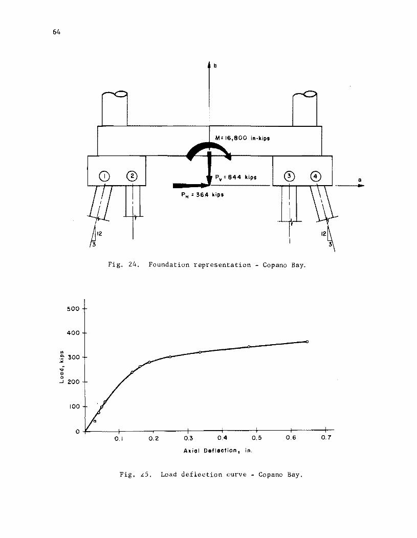
64
500
400
II>
.~ 300 .Jt;
"0 l:I o ...J 200
100
b
® PH : 3614 kips
Fig. 24. Foundation representation - Copano Bay.
o~-----+------+------+--------~-------+------+-----~-0.1 0.2 0.3 0.4 0.5 0.6 0.7
Alial Deflection tin.
Fig. L5. Load deflection curve - Copano Bay.
a ..

65
TABLE I. PILE LOCATION INFORMATION - COPANO BAY
Pile a b No. Piles Batter Location Coordinate Coordinate at
(in. ) (in. ) Location (radians)
1 -126 0 1 -0.244
2 - 90 0 2 0.0
3 + 90 0 2 0.0
4 +126 0 1 +0.244
TABLE II. PILE LOADS AND MOVEMENT - COPANO BAY
Pile Axial Load Lateral Load Moment Axial Lateral Location per Pile per Pile per Pile Movement Movement
(kips) (kips) (in. -kips) (in. ) (in. )
1 78.7 1.7 -253.3 0.0397 0.1134
2 133.4 1.5 -218.9 0.0689 0.1004
3 156.5 1.5 -218.8 0.0843 0.1004
4 193.6 1.1 -155.2 0.1091 0.0763

66
After considering boring logs from the vicinity of the bent and after
a review of triaxial data, a variation of cohesion with depth was assumed and
used for predicting lateral pile-soil interaction. This assumed distribution
of cohesion along the pile length is shown in Fig. 26. The depth given is
the distance from the soil surface. The top of the piles are located at the
water surface which is 10 ft above the soil surface. The scourline is assumed
to be 5 ft below the soil surface. The saturated unit weight of the soil is
taken as 92 pcf, and the consistency is soft.
A solution was obtained for this problem by using the program BENTI
which was described in Chapter V. The movement of the bent is described by
the following movements of the origin of the a-b coordinate system.
tV 7.664 x 10- 2 in.
tH = 1.004 x 10- 1 in.
a = 8.536 x 10- 5 radians
The loads transferred to each pile and the movements of each pile top are tab
ulated in Table II. The forces and movements at the pile tops are related to
the x-y coordinate system set up for each pile.
The deflection of the a-b coordinate system defines the equilibrium
position for the structure. When the foundation is in this position the piles
exert on the foundation the given forces and moments which satisfy the three
equilibrium equations. A complete listing of the coded input and output are
presented in Appendices E and F.
If the movement of the structure and the loads carried by each pile
are considered, it would appear that the design is conservative. This is
probably true, but it should be pointed out that factors such as settlement
caused by consolidation and cyclic loading have not been considered.
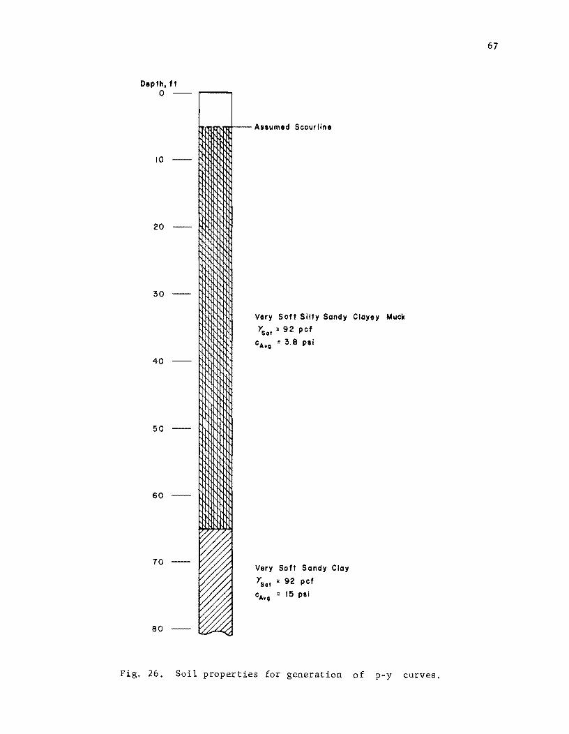
Depth, If o --
10 --
20 --
30 --
40 --
50 --
60
TO --
eo
h" .... ..,. .... ,...,>+-- Assumed Scourline
Very Soft Silty Sandy Clayey Muck
>'sot : 92 pcf
cAv; = 3.8 psi
Very Soft Sandy Clay
Ysot : 92 pcf
CAVil = 15 psi
Fig. 26. Soil properties for generation of p-y curves.
67

68
HOUSTON SHIP CHANNEL
The second example considered will be one of the bents used in a
bridge across the Houston Ship Channel. The bridge is located in Harris County
on Interstate Highway 610. Details of the bent analyzed are shown in Fig. 27.
The bent is reinforced concrete and is supported by 142 - 18 in. square pre
cast-prestressed concrete piles. The piles in this example are battered
parallel to the roadway to resist horizontal loads from the superstructure.
It is assumed that the 7 ft thick pile cap provides sufficient rigidity so
that the assumption of plane movement is valid.
The geometry necessary for describing the foundation for the computer
solution is shown in Fig. 28 and Table III. The coordinate system and the
loads on the structure are also shown in the figure. The piles have an effec
tive flexural rigidity of 4.374 x 10¹⁰
lb-in.2
(assuming a modulus of elas
ticity of concrete of 5 x 10⁶
psi) and a length of 44 ft.
No axial load-deflection curves obtained from load tests are available
for the piles used in the bent. Because of this it was necessary to estimate
the axial behavior of the piles. The ultimate bearing capacity of the piles
was estimated as 650 kips in compression and 600 kips in tension. The ulti
mate deflection is estimated as 0.5 in. The load-deflection relationship is
assumed to be linear resulting in a curve as shown in Fig. 29.
The properties of the soil used for predicting the lateral pile-soil
interaction were obtained from highway department borings. The properties
used for generation of p-y curves are shown in Fig. 30. It should be pointed
out that the profile shown is a simplification of the actual profile. The top
13 ft of soil, defined as very dense sandy silt, will be treated as a sand
when p-y curves are generated. That is, it will be treated as a cohesion
less material. The bottom 31 ft, defined as very stiff silty clay, will be

... -o I'-
t ... -
... -
f
4ft 4 ft 4ft 4ft
8 ft
~----------- 46 a t 3ft 6 in. = 161 ft -----------~.~I 0 0 0 0 D C 0 ,--, r, " r1 ,..-, ,..--,
0 10 1 , 1 , , , 1 , 1 III 01 0 1 1 1 1 , , , 1 , , , 1
0 q 0' I , , , , , ,
~ _____ ~.J D Ie 0 1.. _______ .... L. ________ ~ L ________ ~ L. _______ ~ , I cr-------i ['"--------1 r-------j i-------i ['"-----11-10 P 0 q 0
: 0 : : : l : : : I : r1 C: D 0 ... __ ~ ... _~ _.J L_.J L._... L __ ..1
0 0 D 0 0 D 0
Fig. 27. Houston Ship Channel bent.
f
2 2
~ 3ft 6in.
5 ft
5ft 5ft 5ft
5ft
i 3ft 6in.

70
b
in-kips
PH : 1,126 kips Pv: 27,600 kips
12 12 12
1
®
Fig. 28. Foundation representation - Ship Channel.
a •
C
c 0 -u u -., 0
Load, kip.
100 o O~~-+----+---~----~--~~--~----+-
700 200 300 400 500 600
0.5
1.0
1.5
Fig. 29. Estimated axial load deformation curve - Ship Channel.
Depth, ft
0--
10 ---
20 ---
30 --
40 ---
Very Dense Sandy Silt
YSat : 115 pcf
f/J : 35°
Very Stiff Silty Clay
YSat : 92 pcf
c : 14 psi
Note: Water Table Above Section Shown
Fig. 30. Soil properties for p-y curves - Ship Channel.
71

72
TABLE III. PILE LOCATION INFORMATION - SHIP CHANNEL
Pile a b No. Piles Batter Location Coordinate Coordinate at
(in. ) (in. ) Location (radians)
1 -150 0 24 -0.166
2 - 90 0 23 -0.083
3 - 30 0 24 -0.042
4 30 0 24 0.042
5 90 0 23 0.083
6 150 0 24 0.166
TABLE IV. PILE LOADS AND MOVEMENTS - SHIP CHANNEL
Pile Axial Load Lateral Load Moment Axial Lateral Location per Pile per Pile per Pile Movement Movement
(kips) (kips) (in. -kips) (in. ) (in. )
1 106.3 3.3 -46.0 0.0818 0.0474
2 143.6 2.5 0.4 0.1104 0.0425
3 178.3 2.0 32.8 0.1372 0.0390
4 214.5 0.3 122.1 0.1650 0.0263
5 248.3 0.2 83.8 0.1910 0.0174
6 281. 5 0.0 -15.2 0.2165 -0.0026
treated as a clay. That is, it will be treated as a frictionless material.
Depths given are measured from the top of the pile. From the given soil
properties, p-y curves are generated. These are shown in Appendix F.
A solution was obtained for the Ship Channel problem by using the
program BENT1. The movement of the bent, when loaded, is described by the
following movements of the origin of the a-b coordinate system.
6V 1.512 X 10- 1 in.
6H 3.321 x 10- 2 in.
a 4.183 x 10⁻⁴ radians.
73
The loads transferred to each pile and the movements of each pile top are tab
ulated in Table IV. The forces and movements at the pile tops are related to
the x-y coordinate systems set up for each pile. A complete set of coded
input is given in Appendix E. The output is shown in Appendix F.
The small deflections and loads obtained for the piles would tend to
indicate that the design is conservative. This is probably true, and is to
be expected. But, it should be pointed out that a number of factors, such as
consolidation and cyclic loading have not been considered. It must also be
pOinted out that the load deflection curve used is only a rough approximation.
The value used for ultimate load is probably fairly reliable, but the deflec
tion at which the load stops increasing is only an educated guess. Because of
this a linear variation of load with movement was considered to provide suffi
cient refinement. The effect of this will be reflected in the loads and de
flections obtained for the piles. The loads obtained will probably be fairly
accurate but the accuracy of the movements obtained will depend on the accu
racy of the value which was assumed for the deflection at which the load stops
increasing.

!!!!!!!!!!!!!!!!!!!"#$%!&'()!*)&+',)%!'-!$-.)-.$/-'++0!1+'-2!&'()!$-!.#)!/*$($-'+3!
44!5"6!7$1*'*0!8$($.$9'.$/-!")':!
CHAPTER VII
SUMMARY AND CONCLUSIONS
The UT method, for analyzing two-dimensional pile supported founda
tions, is the most complete method which has been considered in this study.
The improvements over the other methods considered are summarized in the
conclusions to Chapter II. The major improvements are the ability to consi
der the nonlinear load-deflection relationships for the piles and the ability
to consider any type of pile-to-foundation connection.
The consideration of only two-dimensional configurations and the
assumption that the pile heads remain in the same plane before and after load
ing are not serious limitations of the method. For a great many practical
engineering problems these two requirements are approximated to a degree so
that the results obtained provide useful information.
The method assumes that the piles in the bent behave as individually
loaded piles. The problem with the method is not in the method of computation
but rather with predicting the behavior of the individual piles in the bent.
This problem may be considered in two parts.
In the first consideration, methods must be available for predicting
the lateral and axial behavior of the individual piles. This subject is dis
cussed in Chapter IV and it was concluded that a load test is the only proven
way to determine axial behavior, and that the method presented for predicting
lateral interaction is based on theoretical considerations and a limited
amount of field data.
The second consideration is the spacing of the piles. The spacing of
the piles at which the behavior of one pile is influenced by the surrounding
piles is not well defined. There is no general agreement as to the minimum
75

76
spacing at which this influence is felt or the magnitude of the influence.
This factor must be considered if the solutions obtained are to be meaningful.
since it has been assumed that the piles act independently.
Other factors which should be considered are the effect of axial load
on lateral behavior and lateral load on axial behavior. An attempt has been
made to include the effect of axial load on lateral behavior by considering
the effect of axial load on the deflected shape o~ the pile. The axial load
is considered to be constant over the entire length of the pile. This is an
incorrect assumption since some load is removed by skin friction. It is felt
that no further refinement is justified because of the inability to accurately
predict the variation with depth and because the effect on the accuracy is
considered insignificant. No provision is made for considering the efffect of
lateral load on axial behavior. Any adjustment would have to be made through
the axial load-deflection curve.
The UT method is a rational approach to a complicated problem. It
can provide information which will aid the designer and it will aid in under
standing the mechanics of a pile supported foundation. This information
should be used only after careful consideration is given to the assumptions
involved in providing input information. Research will eliminate many of the
uncertainties involved, but for the present it must be remembered that the
accuracy of the solutions obtained depend on the accuracy of the input. infor-
mation.

APPENDIX A
GUIDE FOR DATA INPUT

!!!!!!!!!!!!!!!!!!!"#$%!&'()!*)&+',)%!'-!$-.)-.$/-'++0!1+'-2!&'()!$-!.#)!/*$($-'+3!
44!5"6!7$1*'*0!8$($.$9'.$/-!")':!

BENTI GUIDE FOR DATA INPUT -- Card forms
IDENTIFICATION OF PROBLEM (1 alphanumeric card per problem)
FOUNDATION LOAD AND CONTROL DATA (1 card per problem)
PV PH TM TOL KNPL KOSC
10 20 30 40 45 50
P\l - VERTICAL LOAD ON FOUNDATION
PH - HORIZONTAL LOAD ON FOUNDATION
TM - MOMENT ON FOUNDATION
TOL - ITERATION TOLERANCE
KNPL - NUMBER OF PILE LOCATIONS
KOSC - SWITCH TO CONTROL OSCILLATING SOLUTION (Set equal to 1 if solution oscillates. Set equal to 0 for normal use.)
CONTROL DATA FOR PILE LOCATIONS (1 card per pile location)
DISTA DISTB THETA POTT KS KA
10 20 30 40 45 50

!!!!!!!!!!!!!!!!!!!"#$%!&'()!*)&+',)%!'-!$-.)-.$/-'++0!1+'-2!&'()!$-!.#)!/*$($-'+3!
44!5"6!7$1*'*0!8$($.$9'.$/-!")':!

DISTA - HORIZONTAL COORDINATE OF PILE TOP
DISTB - VERTICAL COORDINATE OF PILE TOP
THETA - PILE BATTER
POTT - NUMBER OF PILES AT A LOCATION
KS - IDENTIFIER TO RELATE PILE TO p-y CURVE
KA - IDENTIFIER TO RELATE PILE TO AXIAL LOAD SETTLEMENT CURVE
Note: KS and KA are necessary for selecting the correct set of p-y curves and axial load settlement curve for a pile. This option is made available because for some problems all piles may not behave alike. These two variables correspond to IDPY and IDEN which are input with p-y and load settlement data.
CONTROL DATA FOR PILES (KNPL sets per problem)
NN HH DPS NDEI TC FDBET E ( 1 card per
I I location) 6 10 20 30 36 40 48 50 60 70
RRI XXi XX2 (NDEI cards per pile location)
10 20 30
NN - NUMBER OF INCREMENTS
HH - INCREMENT LENGTH
DPS - DISTANCE FROM PILE TOP TO SOIL SURFACE
NDEI - NUMBER OF DIFFERENT EI VALUES IN PILE
TC - ALPHANUMERIC DESIGNATION FOR TOP CONNECTION OF PILE (FIX - Fixed connection, PIN - Pinned connection, RES - Restrained connection)

This page replaces an intentionally blank page in the original --- CTR Library Digitization Team

FDBET - ROTATIONAL RESTRAINT (Not necessary unless TC RES)
E - PILE DIAMETER OR WIDTH
RRI - FLEXURAL STIFFNESS (EI) OF A SECTION
XXl - DISTANCE FROM PILE TOP TO TOP OF SECTION
XX2 - DISTANCE FROM PILE TOP TO BOTTOM OF SECTION
CONTROL DATA FOR SOIL PROPERTIES (1 card per problem)
NKA NKS KOK
6 10 16 20 26 30
NKA - NUMBER OF LOAD SETTLEMENT CURVES
NKS - NUMBER OF SETS OF p-y CURVES
KOK - SWITCH FOR INPUT OF p-y CURVES (KOK 0 p-y curves input, KOK = 1 p-y curves generated)
CONTROL AND DATA FOR AXIAL LOAD SETTLEMENT CURVES (NKA sets per problem)
IDEN 10 (1 card per curve)
6 10 16 20
zzz SSS (10 cards per curve)
10 20

This page replaces an intentionally blank page in the original --- CTR Library Digitization Team
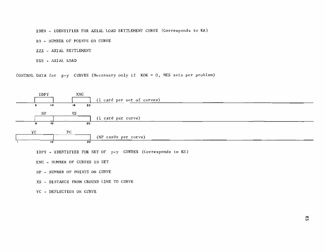
IDEN - IDENTIFIER FOR AXIAL LOAD SETTLEMENT CURVE (Corresponds to KA)
10 - NUMBER OF POINTS ON CURVE
ZZZ - AXIAL SETTLEMENT
SSS - AXIAL LOAD
CONTROL DATA for p-y CURVES (Necessary only if KOK = 0, NKS sets per problem)
IDPY KNC (1 card per set of curves)
6 10 16 20
NP XS
I (1 card per curve) 6 10 20
YC PC (NP cards per curve)
10 20
IDPY - IDENTIFIER FOR SET OF p-y CURVES (Corresponds to KS)
KNC - NUMBER OF CURVES IN SET
NP - NUMBER OF POINTS ON CURVE
XS - DISTANCE FROM GROUND LINE TO CURVE
YC - DEFLECTION ON CURVE
co VI

This page replaces an intentionally blank page in the original --- CTR Library Digitization Team
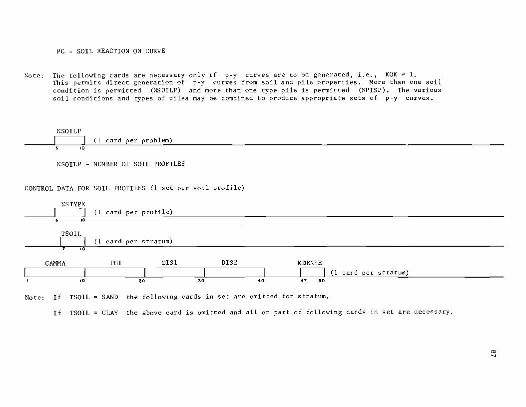
PC - SOIL REACTION ON CURVE
Note: The following cards are necessary only if p-y curves are to be generated, i.e., KOK = 1. This permits direct generation of p-y curves from soil and pile properties. More than one soil condition is permitted (NSOILP) and more than one type pile is permitted (NPISP). The various soil conditions and types of piles may be combined to produce appropriate sets of p-y curves.
NSOILP
I (1 card per problem) 6 10
NSOILP - NUMBER OF SOIL PROFILES
CONTROL DATA FOR SOIL PROFILES (1 set per soil profile)
NSTYPE I (1 card per profile)
6 10
TSOIL I I (1 card per stratum)
7 10
GAMMA PHI DISl DIS2 KDENSE
(1 card per stratum) 10 20 30 40 47 50
Note: If TSOIL SAND the following cards in set are omitted for stratum.
If TSOIL CLAY the above card is omi tted and all or part of following cards in set are necessary.

This page replaces an intentionally blank page in the original --- CTR Library Digitization Team

GAMMA SHEARS DISI DIS2 INFO ICON (1 card per stratum)
10 20 30 40 46 so 56 60
Note: If INFO o following cards in set are omitted. If INFO = 1 they are necessary.
NCURVS I (1 card per stratum) 6 10
DIST NPOINT I (1 card per stress strain curve)
10 16 20
SIGD EP (NPOINT cards per curve)
10 20
NSTYPE - NUMBER OF STRATA IN PROFILE
TSOIL - ALPHANUMERIC DESIGNATION OF TYPE SOIL IN STRATUM (SAND OR CLAY)
GAMMA - UNIT WEIGHT OF SOIL
PHI - ANGLE OF INTERNAL FRICTION FOR SAND
DISI - DISTANCE FROM GROUND LINE TO TOP OF STRATUM
DIS2 - DISTANCE FROM GROUND LINE TO BOTTOM OF STRATUM
KDENSE - ALPHANUMERIC DESIGNATION FOR RELATIVE DENSITY OF SAND (DENSE, MEDUM OR LOOSE)
SHEARS - COHESION OF CLAY
00 \0

This page replaces an intentionally blank page in the original --- CTR Library Digitization Team
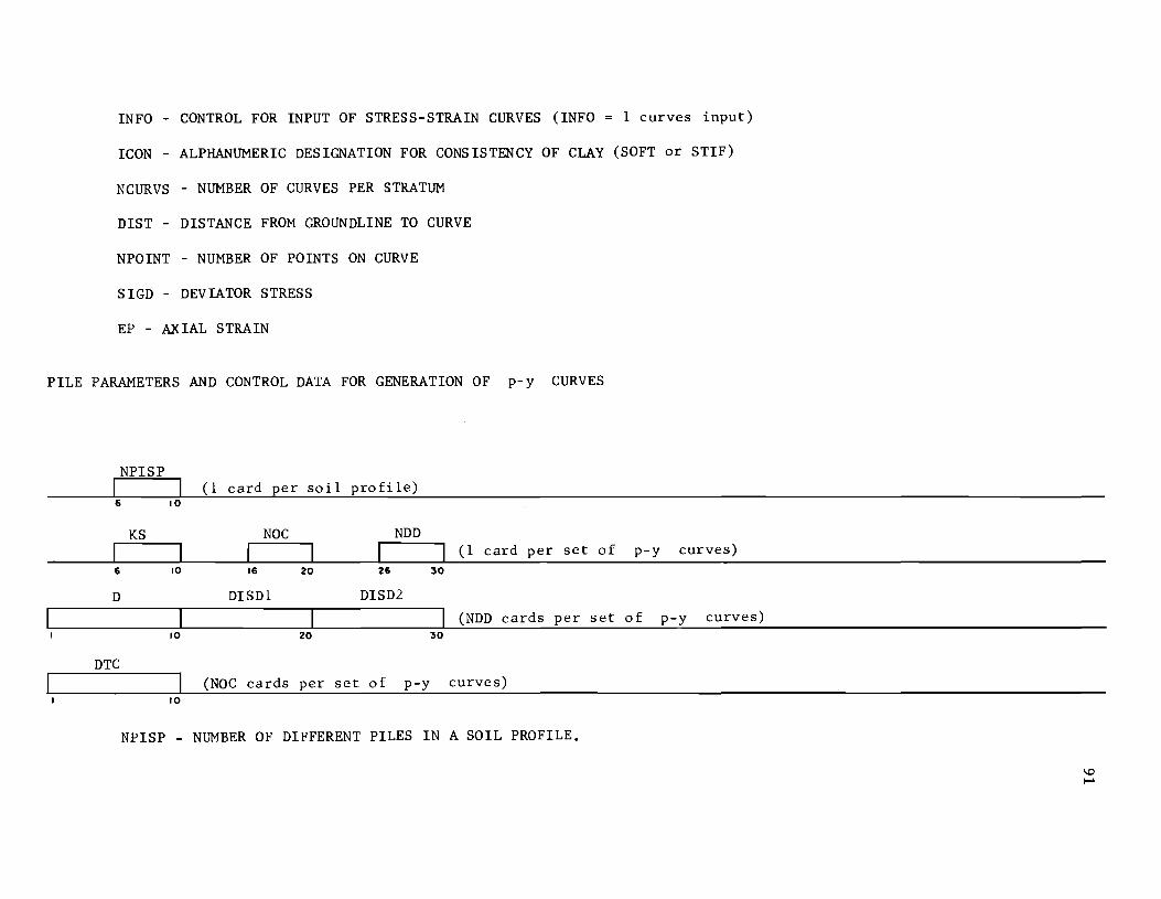
INFO - CONTROL FOR INPUT OF STRESS-STRAIN CURVES (INFO = 1 curves input)
ICON - ALPHANUMERIC DESIGNATION FOR CONSISTENCY OF CLAY (SOFT or STIF)
NCURVS - NUMBER OF CURVES PER STRATUM
DIST - DISTANCE FROM GROUNDLINE TO CURVE
NPOINT - NUMBER OF POINTS ON CURVE
SIGD - DEVIATOR STRESS
EP - AXIAL STRAIN
PILE PARAMETERS AND CONTROL DATA FOR GENERATION OF p-y CURVES
NPISP I I (1 card per soil profile) 6 10
KS NOC NDD (1 card per set of p-y curves)
6 10 16 20 26 30
D DISDl DISD2
(NDD cards per set of p-y curves) 10 20 30
DTC (NOC cards per set of p-y curves)
10
NPISP - NUMBER OF DIFFERENT PILES IN A SOIL PROFILE.

This page replaces an intentionally blank page in the original --- CTR Library Digitization Team

KS - IDENTIFIER FOR SET OF p-y CURVES
NOC - NUMBER OF CURVES IN SET
NDD - NUMBER OF DIFFERENT DIAMETERS USED FOR p-y CURVES
D - PILE DIAMETER
DISDl - DISTANCE FROM TOP OF PILE TO TOP OF SECTION
DISD2 - DISTANCE FROM TOP OF PILE TO BOTTOM OF SECTION
DTC - DISTANCE FROM TOP OF PILE TO p-y CURVE
STOP CARDS (2 blank cards at end of run)
GENERAL PROGRAM NOTES
All input values in units of pounds, inches and radians. AilS-space words are right justified integers, unless specified as on alphanumeric word. All lO-space words are floating-point decimal numbers. Data cards must be stacked in proper sequence. Where a group of cards are referred to as a set, the cards in the set must be stacked in the sequence shown. Sets are then stacked. Several problems may be run by stacking data for additional problems behind first problem. Two blank cards behind last problem stops the program.
10
10

This page replaces an intentionally blank page in the original --- CTR Library Digitization Team
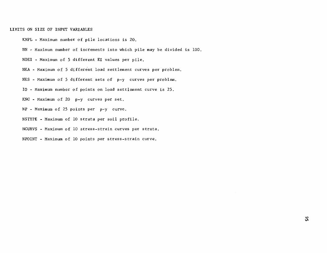
LIMITS ON SIZE OF INPUT VARIABLES
KNPL - Maximum number of pile locations is 20.
NN - Maximum number of increments into which pile may be divided is 100.
NDEI - Maximum of 5 different EI values per pile.
NKA - Maximum of 5 different load settlement curves per problem.
NKS - Maximum of 5 different sets of p-y curves per problem.
10 - Maximum number of points on load settlement curve is 25.
KNC - Maximum of 20 p-y curves per set.
NP - Maximum of 25 points per p-y curve.
NSTYPE - Maximum of 10 strata per soil profile.
NCURVS - Maximum of 10 stress-strain curves per strata.
NPOINT - Maximum of 10 points per stress-strain curve.

This page replaces an intentionally blank page in the original --- CTR Library Digitization Team

APPENDIX B
FLOW CHART FOR BENTI

!!!!!!!!!!!!!!!!!!!"#$%!&'()!*)&+',)%!'-!$-.)-.$/-'++0!1+'-2!&'()!$-!.#)!/*$($-'+3!
44!5"6!7$1*'*0!8$($.$9'.$/-!")':!
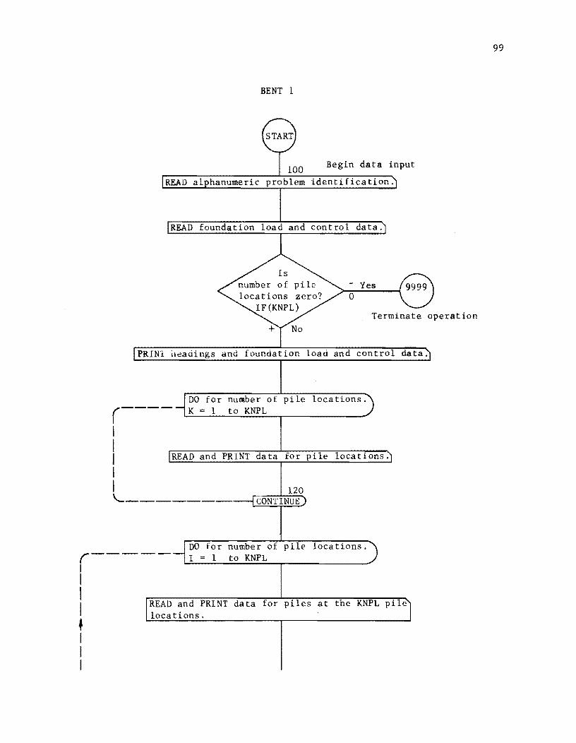
BENT 1
Begin data input
problem identification.
READ foundation load and control data.
- Yes o
Terminate operation
PRINl ~eadings and foundation load and control data.
DO for number of pile locations. (---- K = 1 to KNPL
I I I I
READ and PRINT data for pile locations.
I '--------
120 CONTINUE
r----I
DO for number of pile locations. I = I to KNPL
I I I • I I I
READ and PRINT data for piles at the KNPL pile locations .
99

100
I I 00 for
I number of different stiffness
• r--_.- values for piles at location.
I I I I I I
I I I I \..._~--
J = 1 to NDST = NDEI (1)
IREAD pile st iffness information·l
150 ------ CONTINUE)
r---- 00 for number of pile locationS) - M = 1 KNPL to
IPRINT heading for piles at location M.1
DO for number of stiffness values
r--_.- for the piles at location M. N = 1 to NEI = NDEI(M) I
I I I I
I PRINT stiffness data for piles at location M.~
"--~--15.5
------ CONTINUE)
I READ control data for input of soil interaction, parameters.
r---I I I I + I I
DO for number of axial load Inp ---- deflection curves to be input. loa
L = 1 to NKA cur
IREAD and PRINT curve of points on curve.
identifier and numberi
ut of axial d deflection ves.

I I I I 00 for number of points on r---- curve L. LL = 1 to 10
I I
LI I 160
---~ READ and PRINT load and corres
+ No
,----I
DO for number of sets of p-y curves to be input. K = 1 to NKS
Input of p,..y curves.
I I I I I
READ and PRINT set identifier and number of curves in set K.
DO for number of curves r-------- in set K. I = 1 to KNC
I I I I
READ and PRINT number of points on the curve and the depth to curve I. PRINT headings.
II r - DO for number of points on curve 1.
L = 1 to NT = NP(IDPY,I)
I I I I I I
and PRINT deflection and corresponding oil reaction.
I I L L 130 _ _L _____ CONTINUE
GO TO 152
101

102
151
CALL MAKE
152
CONTINUE
SET indices KFLAG, KEY, KSW, ITER, DV, DR and ALPAA equal to zero.
iteration data.
GO TO 325
310
CONTINUE
ITER ITER + 1
SUBROUTINE MAKE generates p-y curves from soil properties.
Begin computation procedure.
Check closure for foundation movements.
+ No
+ No
+ No

325
DO for number of pile locations. r--- -- I = I to KNPL
,-I I I t I I I I
Calculate XT and YT for piles at location I.
Is this the initial
itera tion ? IF (KSW)
Set XT, YT and BC2 for initial iteration.
GO TO 340
Calculate PT, FMT, and set BC2 for piles at location 1.
340
ND KA (1), IT = II (ND)
+
DO for number of points on load deflection curve for piles at location I. J = 2 to IT
103
No
No

104
t \_------
PRINT error message.
GO TO 100 I---------~
a No +
PRINT error message.
GO TO 100
365 Calculate PX and FJX(I)
No a
PRINT headings and output for pile location I.
400 SUBROUTINE COM 62 solves laterally loaded pile for given boundary conditions.

I
• I I I
FJM (I) FJMO FJY (I) FJYO
410 '--------- CONTINUE
+ Yes
DHT DH DVT DV AT = ALPHA
DO for number of pile locations. r---- J = 1 to KNPL
I I I I I I
For each pile location calculate the influence of the piles on the foundation movement as the coefficients AA(J), BB(J), CC (J ), DD (J ), and EE (J ) .
l _______ r----_---'----4-'--3--=O ........
Calculate and PRINT the foundation movement (ALPHA, DV and DH) by Kramer! s Rule.
105

106
o No
o No
Average foundation movements with movements from previous iteration.
GO TO 310
9999 CONTINUE

107
SUBROUTINE COM62.
This subroutine solves laterally loaded pile for given boundary conditions.
y Set indices and constants. H = HH (I TYPE ) , N :: NN(ITYPE) NP3 .: N+3, ITER = 1, K = 1
DO for NP3 stations along Th - pile. J = 3 to NP3 se va it st
r---I I I Set initial values for soil modulus
ES (J) , pile stiffness R(J) and latera 1 deflection Y (J) . If EI distribution does not cover entire pile length an error message is
I I I I printed and set KEY - 1.
I I \..._------
1051 CONTINUE)
r---I I I I J I I
1052 Calculate A&B coefficients for
the bottom two stations of pile.
DO for all but bottom two
- stations of pile. J = 4 to Nl :: NP3-2
Calculate A(KT) and B(KT) where I KT = NP3 - J + 2.
Ca fo fi eq
is DO loop ts initial lues to get eration procedure arted.
lculate coefficients r the solution of nite difference uations.

108
Calculate Y(3) and Y(4) which are the deflections of top two stations on pile. Equations used will depend on iteration number and top connection.
o Yes
1065 Calculate Y(3) and Y(4) with YT as second boundary condo
+
@IGQO}T~oj1@OE81DI------~

Calculate Y(3 as second
GO TO 1081
1067 Calculate Y(3) and Y(4) with YT as second boundary condition.
GO TO 1081
1070 Calculate Y(3) and Y(4) with MT as second boundary condition.
GO TO 1081
1071 Calculate Y(3) and Y(4) with ST as second boundary condition.
GO TO 1081
1072 Calculate Y(3) and Y(4) with MT/ST as second boundary condition.
1081 KYCNT = 0
Check closure for
109
lateral pile deflections.
Yes o

110
,--
o
DO for all but top two stations of pile. J = 5 to NP3
Set YTMP = Y(J) and calculate new value for Y(J).
o
KYCNT
'-------
Yes
Yes
Yes o

o No
+ Yes
1095 Set Y(3) = 3.0*E and KSW = 1. Calculate Y(4).
GO TO 1081·
o No
2015 ITER ITER + 1
+ Yes 2016
SUBROUTINE SOIL 2R calculates soil modulus values (ES) for given deflec t ions.
+ Yes
o No
and print
GO TO 2027 r------I
2017 1052
111
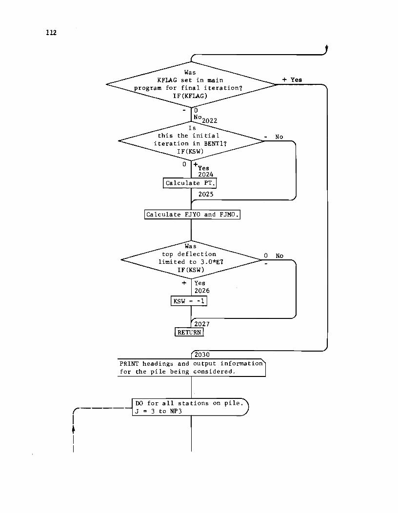
III
2025
Calculate FJYO and FJMO.
2030 PRINT headings and output information for the pile being considered.
r---I • I I
DO for all stations on pile. J = 3 to NP3
+ Yes
No
o No

I I • I I I
Calculate and PRINT for each station along the pile the depth, deflection, moment, soil modulus and soil reaction.
"---------
113

114
SUBROUTINE SOIL 2R
This subroutine calculates soil modulus values (ES) from given lateral
deflections (Y).
r-I I I I I I
I I I 4
DO for number of stations along the pile. J = 3 to NP3
ZJ=J-3 Z = ZJ*H - DPS(ITYPE)
3010
ES (J) = 0.0
+ No o
GO TO 3090 1---------1
than
Locate p-y curves above and below stationJ.
Less than +

No
r-----1 I
Set KEY • 1
RETURN]
GO TO 3035
3035 YA ABS (Y (J ) )
3036
YA 1. OE-lO
3037 DO for curves above and below station J. I = M to K
o No
+
•
115
Locate points behind and ahead of YA on each p-y curve and compute ES on each curve.

116
I I I I I I I I I I I I I I I I t I I I
0
No 0
• I I I I I
3045 L = L + 1
GO TO 3065
GO TO 30651-------_.1
3060 Calculate PI from values on curve above and below YA.
3065 Calculate soil modulus EST(I).
3070 \..._------- CONTINUE
+

I I I I I I I
• I I I I I I I I I
+ No
117
Interpolate between curves to obtain correct soil modulus ES(J)
GO TO 30901----------_+_ __
Calculate ES(J) by interpolation between soil modulus values for p-y curves above and below station J.
'------------

118
SUBROUTINE MAKE
This subroutine generates p-y curves from soil properties.
START
READ the number of soil profiles for which p-y curves are to be generated (NSOILP).
Set control values for type soil, density of sand and consistency of clay.
,----I
DO for number of soil profiles for which p-y curves are to be generated. ISP = 1 to NSOILP
I t READ the number of layers of soil in
profile (NSTYPE).
,---I
DO for number of layers in the profile. 1ST = 1 to NSTYPE
the
• I READ and PRINT type of soil in layer 1ST.
I I I I I I I
soil in the layer sand? IF(TSOIL(IST)
.EQ. TESTl)
No
Begin data input.

t ~ I I I I I I
500
READ and PRINT properties of sand in layer.
Set coefficient of earth pressure and constant for slope of p-y curves.
GO TO 510
a medium dense condition? IF (KDENSE
!TESTB)
Set coefficient of earth pressure and constant for slope of p-y curves.
No
o
~G_O __ T_O_5_1_0 __ ~--------~~
Set coefficient of earth pressure and constant for slope of p-y curves for loose condition.
GO TO 510
507 READ and PRINT properties of clay in layer.
119

120
I I I I t
I I I I I I I ~
+ No o
READ and PRINT number of stress-strain curves to be input.
r-- DO for number of curves input. JJ = 1 to NCUR
~ I I I I
READ and PRINT depth to curve and number of points on the curve.
I DO for number of points on r----I curve JJ. JK = 1 to NPZ
i + I : I I
READ and PRINT deviator stress and strain for each point.
I I LL~ ___ _ 510
CONTINUE
READ number of different types of piles for which p-y curves are to be generated for the soil profile being considered.
DO for number of piles for ,-____________ ~ which p-y curves are to
be generated. JP = 1 to NPISP I
+ I I I

121
I , I I I I READ identifier for set of curves, number of curves
I to be generated and number of different diameters
I considered.
I I I I I PRINT headings.
I + I I I
DO for number of di fferent r-- diameters.
I I + I • l_ READ and PRINT
511 diameter and depths.
I I I DO for number of curves to be
I ,--- generated. IJK = 1 to NOe
I I I
I • READ and PRINT distance to the curve. I I I
I I DO for number of layers in
I I i-- profile. IF'S = 1 to NSTYPE
I I I I I + I I I I I I 0 Yes
+
I I I I I I L ____ I I
I I I I I Is
I I soil in layer IFS No sand? IF (TSOIL(IFS)
I I .EQ. TESTl)
I I I I I I

122
I
I I
• I I I I I I 4 I I I I I I I I • I I
I r-I I I I
4 I I I I
o Yes
Calculate a weighted average of the densities of the soil above the location of the curve.
GO TO 518
517 Set AGAM GAMMA (IFS ) .
518 DO for number of different diameters of pile for which curve is generated. IPT = 1 to NDD
diameter under considlocated at depth of IF(DISD2(IPT)- DTC
(KS ,UK))
"-------520
Set DIA = D(IPT) and calculate ALPHA and ES.
slope of curve (ES) zero?
IF (ES)
+ No
o Yes +
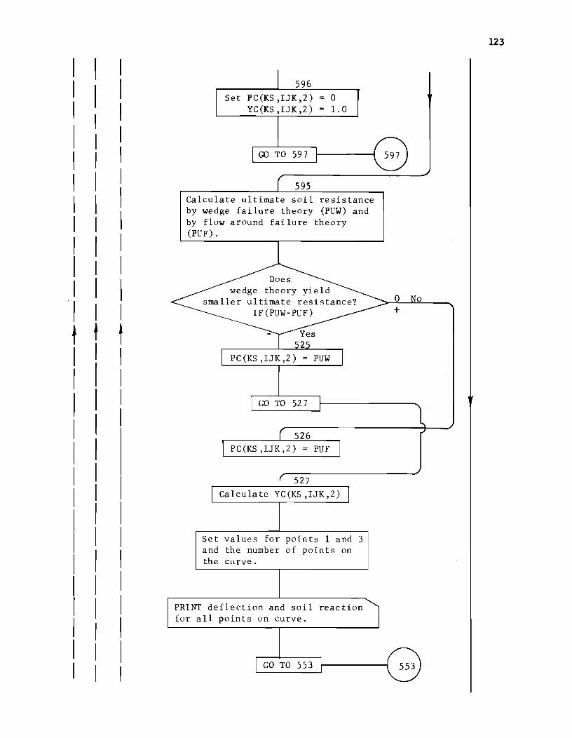
t t t
596
Set PC(KS,IJK,2) a YC(KS,IJK,2) 1.0
GO TO 597
595
Calculate ultimate soil resistance by wedge failure theory (PUW) and by flow around failure theory (PUF) .
GO TO 527
526
PC(KS,IJK,2) = PUF
527
Calculate YC(KS,IJK,2)
Set values for points 1 and 3 and the number of points on the curve.
PRINT deflection and soil reaction for all points on curve.
GO TO 553
123
o 0
+

124
I I I I I 4
I I I I I I I I I I I-
I I I I I I I + I I I I
Set value according to consistency of clay.
534
+ No
Yes 535 Set AGAM GAMMA (IFS)
+ Yes
Generation of p-y curves without stre •• -strain curves.
GO TO 538 1--------_
rI I ~ I I I I
536 Calculate a weighted average of the density of the soil above the location of the curve.
538 DO for number of different diameters of pile for which curve is to be genera ted. IPT = 1 to NDD
diameter under consideration located at depth of
IF(DISD2(IPT)- DTC (KS,IJK))
'-------
o Yes +

I I I I I I I I I I I I I I I I I I I I ~
540
Set DrA = D(IPT) and SIGSO :::; SHEARS (IFS). Calculate PUW, PUF and DIFF.
+ No
Set values of soil resistance for points 11 and 12 equal to PUF and set corresponding values of deflection. Also set IPOINT (KS .IJK) '" 12.
GO TO 546
,-I
DO for ITO 1 to 9
I I I ~qU'l I I L
Calculate soil reaction Q(ITO).
DIFF = DIFF/10.O STUP :::; 9.0
Number of points on limited to 12.
er
125

126
,-- DO for ITO 1 to 9.
Calculate soil reaction Q (ITO).
562 Set IPOINT (KS,IJK) 3 and values for points 2 and 3.
GO TO 5461-------~
544 Set MPOINT = IPOINT(KS,IJK) = l2-ITO and KZ = MPOINT-l. Set values for points MPOINT and KZ.
GO TO 546
545 Set MPOINT = IPOINT(KS ,IJK) = 13-ITO and KF = MPOINT-l. Set values for points MPOINT and KZ.
546 CONTINUE
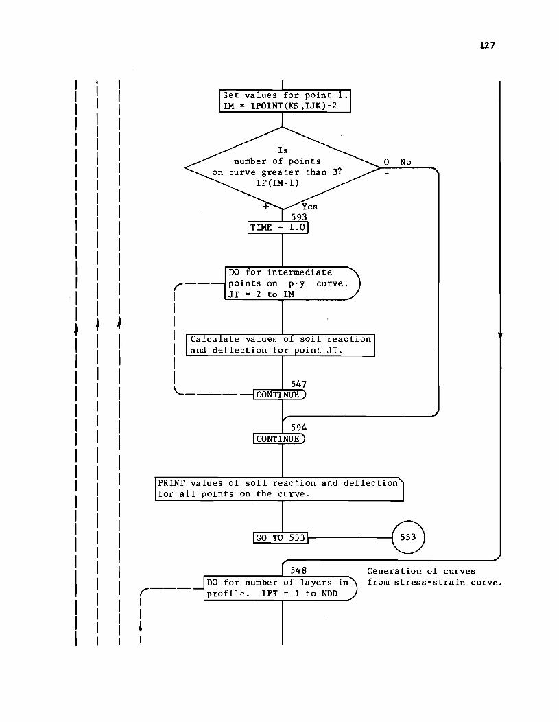
,-I I I I I I
Set values for point 1. 1M = IPOINT(KS,IJK)-2
DO for intermediate points on p-y JT = 2 to 1M
curve.
reaction oint JT.
I \.._---
547 CONTINUE
594 CONTINUE
o No
PRINT values of soil reaction and deflection for all points on the curve.
GO TO 553
127
548 Generation of curves from stress-strain curve. r--
I
DO for number of layers in profile. IPT = 1 to NOD
I , I

128
I I I I I I I
I I I I I I I I I I I I I I I I I I I I I I I I I I I I I I I ~ + 4
I I I
I I , I I I I No
I 549 '------- CONTINUE
Set DIA = NUG=
00 for number of stress strain ,-- curves for layer. IFC = 1 to
I NUG
I I I I I I I No
I 550 '------- CONTINUE
551 CONTINUE
Set values for point 1. MZ = NPOINT(IFS,IFC)
DO for number of points on stress-strain curve. JT = 2, MZ
0 Yes +
+ Yes 0
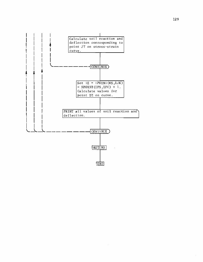
I I I I I I I I I I I I I I I I I I I I I t • • I I I I I I I I I I I I I I I I I I I I I
I I I
I I
• I I I
I Calculate soil reaction and deflection corresponding to point JT on stress-strain curve.
\..------- CONTINUE)
Set IE = IPOINT(KS,IJK) = NPOINT(IFS,IFC) + 1. Calculate values for point IE on curve.
I
PRINT all values of soil reaction and1 deflection. I
"--~-~------- CONTINUE)
I RETURN]
129

!!!!!!!!!!!!!!!!!!!"#$%!&'()!*)&+',)%!'-!$-.)-.$/-'++0!1+'-2!&'()!$-!.#)!/*$($-'+3!
44!5"6!7$1*'*0!8$($.$9'.$/-!")':!
APPENDIX C
GLOSSARY OF NOTATION FOR BENTl

!!!!!!!!!!!!!!!!!!!"#$%!&'()!*)&+',)%!'-!$-.)-.$/-'++0!1+'-2!&'()!$-!.#)!/*$($-'+3!
44!5"6!7$1*'*0!8$($.$9'.$/-!")':!

133
NOTATION FOR BENTl
THE FOLLOWING VARIABLES ARE INPUT AS DATA FOR THE MAIN PROGRAM
ANUM
PV PH TM TOL
KNPL KOSC
DISTA DISTB THETA POTT KS KA
HH NN DPS NDEI TC
FDBET
RRI XX1
XX2
NKA NKS KOK
IDEN 10 ZZZ SSS IDPY KNC NP XS YC PC E
ALPHANUMERIC IDENTIFICATION--ONE 80 COLUMN CARD DESCRIBING THE PROBLFM VERTICAL LOAD ON BENT THROUGH ORIGIN OF COORDINATES HORIZ LOAD ON BENT THROUGH ORIGIN OF COORDINATES MOMENT APPLIED TO BENT ABOUT ORIGIN OF COORDINATES ITERATION TOLERANCE-~CONTROLS FOR LATERALLY LOADED PILE ROUTINE AND TRANSLATION OF BENT--MULTIPLIED BY 0.001 FOR ROTATION OF BENT NUMBER OF PILE LOCATIONS IN BENT SWITCH TO CONTROL OSCILLATING SOLUTIONS--SET TO ZERO FOR NORMAL USE--IF BENT MOVEMENTS OSCILLATE SET EQUAL TO ONE HORIZONTAL COORDINATE OF PILE HEAD VERTICAL COORDINATE OF PILE HEAD BATTER OF PILE MEASURED FROM VERTICAL--NEGATIVE CLOCKWISE NUMBER OF PILES OF A PARTICULAR TYPE AT A PILE LOCATION IDENTIFIER TO RELATE A PILE TO A SET OF PY CURVES IDENTIFIER TO RELATE A PILE TO AN AXIAL LOAD SETTLEMENT CURVE INCREMENT LENGTH FOR PILE NUMBER OF INCREMENTS INTO WHICH PILE IS DIVIDED DISTANCE FROM PILE TOP TO SOIL SURFACE NUMBER OF DIFFERENT STIFFNESS VALUES FOR PILE ALPHANUMERIC DESIGNATION OF MANNER IN WHICH PILE IS CONNECTED TO STRUCTURE--FIx,PIN,OR RES ROTATIONAL RESTRAINT--MOMENT DIVIDED BY ANGLE CHANGE--MAY BE LEFT BLANK IF TC=FIX OR TC=PIN FLEXURAL STIFFNESS CEI) DISTANCE FROM TOP OF PILE TO TOP OF SECTION OF PILE WITH A CERTAIN FLEXURAL STIFFNESS DISTANCE FROM TOP OF PILE TO BOTTEM OF SECTION OF PILE WITH A CERTAIN FLEXURAL STIFFNESS NUMBER OF AXIAL LOAD SETTLEMENT CURVES INPUT NUMBER OF SETS OF P-Y CURVES INPUT--LEFT BLANK IF KOK=l SWITCH FOR INPUT OF P-Y CURVES--KOK=l NUMERICAL p-Y CURVES INPUT--KOK=O p-Y CURVES GENERATED FROM SOIL PROPERTIES IDENTIFIER FOR LOAD SETTLFMENT CURVE NO. OF POINTS ON LOAD SETTLEMENT CURVE SETTLEMENT ON AXIAL LOAD SETTLEMENT CURVE AXIAL LOAD ON AXIAL LOAD SETTLEMENT CURVE IDENTIFIER FOR SET OF P-Y CURVES NUMBER OF CURVES IN A SET OF P-Y CURVES NUMBER OF POINTS ON A P-Y CURVE DISTANCE FROM SOIL SURFACE TO P-Y CURVE DEFLECTION ON P-Y CURVE SOIL RESISTANCE ON P-Y CURVE pILE DIAMETER AT TOP OF PILE

134
THE FOLLOWING VARIABLES ARE INPUT DATA FOR SUBROUTINE MAKE
NSOILP NSTYPE DISl DIS2 TSOIL GAMMA PHI KDENSE SHEARS
INFO
ICON NCURVS DIST NPOINT SIGn FP NPI5P NOC NDD D DISDI DISD2 DTC
NUMBER OF SOIL PROFILES FOR WHICH P-Y CURVES ARE GENERATED NUMBER OF SOIL LAYERS IN A SOIL PROFILE DISTANCE FROM SURFACE TO TOP OF STRATUM DISTANCE FROM SURFACE TO BOTTEM OF STRATUM ALPHANUMFRIC IDENTIFIER FOR TYPE OF SOIL IN A STRATUM UNIT WEIGHT OF SOIL IN A STRATUM ANGLE OF INTERNAL FRICTION FOR A SAND ALPHANUMERIC IDENTIFIER FOR RELATIVE DENSITY OF SAND SHEAR STRENGTH FOR CLAy
VARIABLE TO CONTROL INPU OF STRESS STRAIN CURVES FOR A CLAY--INFO=O NO CURVES INPUT , INFO=l CURVES INPUT ALPHANUMERIC IDENTIFIER FOR CONSISTENCY OF CLAY NUMBER OF STRESS-STRAIN CURVES INPUT DISTANCE FROM SURFACE TO A CURVE NUMBER OF POINTs ON A CURVE DEVIATOR STRESS STRAIN NUMBER OF SETS OF P-Y CURVEs GENERATED FROM A SOIL PROFILE NUMBER OF CURVEs GENERATED FOR A PARTICULAR SET OF CURVES NUMBER OF SECTIONS wITH DIFFERENT DIAMETERS IN A PILE DIAMETER OF A SECTION OF PILF DISTANCE FROM SURFACE TO TOP OF SECTION DISTANCE FROM SURFACE TO BOTTEM OF SECTION DISTANCE FROM SURFACE TO P-Y CURVE
THE FOLLOwING ARE ADDITIONAL VARIABLES USED IN THE MAIN PROGRAM
KFLAG KEY KSW ITER
DV DH ALPHA XT YT BC2
PT FMT PX I FJX FJY FJM DEN AA
ROUTING SWITCH CONTROLLED BY CLOSURE ROUTING sWITCH CONTROLLED BY INVALID SOLUTION ROUTING SWITCH CONTROLLED BY ITERATION NUMBER COUNTER FOR NUMBER OF ITERATIONS--tJSED FOR ITERATION ON FOUNDATION MOVEMENT AND IN COM62 FOR DEFLECTION OF PILE VERTICAL FOUNDATION MOVEMENT HORIZONTAL FOUNDATION MOVEMENT ROTATION OF FOUNDATION ABOUT ORIGIN OF COORDINATE SYSTEM AxIAL DEFLECTION OF PILE TOP LATERAL DEFLECTION OF PILE TOP SECOND BOUNDRY CONDITION APPLIED TO TOP OF THE PILE FOR USE IN COM62--VALUE wILL DEPEND ON TyPE CONNECTION LATERAL LOAD APPLIED TO TOP OF PILF MOMENT APPLIED TO TOP OF PILE AxIAL LOAD APPLIED TO TOP OF PILE IDENTIFIER FOR PILE UNDER CONSIDERATION AXIAL SPRING MODULuS LATERAL SPRING MODULUS--CALCULATED AS FJYO IN COM62 ROTATIONAL SPRING MODULUS--CALCULATED AS FJMO IN COM62 NUMERATOR FOR CRAMERS RULE
,BB ,CC ,DD ,EE COEFFICIENTS USED IN SOLUTION OF EQUILIBRIUM EQUATIONS COEFFICIENTS USED IN SOLUTION OF EQUILIBRIUM EQUATIONS

D5
THE FOLLOWiNG ADDITIONAL VARIABLES ARE USED IN SUBROUTINE MAKE
1ST FKO
IDENTIFIER FOR STRATUM UNDER CONSIDERATION COEFFICIENTS OF EARTHPRESSURE AT REST FOR SAND
AV AGAM DIA ALPHA ES
CONSTANT USED IN CALCULATING COEFFICIENT OF SUBGRADE REACT AVERAGE UNIT WEIGHT OF SOIL ABOVE A POINT PILE DIAMETER ANGLE OF INTERNAL FRICTION DIViDED BY TWO COEFFICIENT OF SUBGRADE REACTION ULTIMATE SOIL RESiSTANCE FROM WEDGE FAILURE ULTIMATE SOIL RESISTANCE FROM FLOW AROUND FAILURE ONE HALF OF STRAIN AT FAILURE ONE HALF OF ULTIMATE DEViATOR STRESS STRAIN AT FAILURE INCREMENT OF STRAIN
PUW PUF EP50 SIG50 EPIOO DIFF STUP SIGA
COUNTER USED TO CALCULATE STRAIN FROM INCREMENT OF STRAIN DEViATOR STRESS
Q SOIL RESISTANCE IPOINT NUMBER OF POINTS ON P-Y CURVE
THE FOLLOWING VARIABLES ARE USED IN SUBROUTINE COM62
ITYPF J Y ES R KYCNT TMOM PLGTH FMO RfS A ,B
S3,S4,S5
IDENTIFIER FOR PILE UNDER COSIIDERATION IDENTIFIFR FOR STATION UNDER CONSIDERATION DEFLECTION AT STATION J SOIL MODULUS AT STATION J piLE STIFFNESS AT STATION J COUNTER USED TO CHECK CLOSURE MOMENT APPLIED TO PILE TOP PILE LENGTH--INCHES MOMENT AT A STATION ALONG THE PILE SOIL RESISTANCE AT A STATION ALONG THE pILE
,C COEFFICIENTS USED IN THE SOLUTION FOR THE DEFLECTED SHAPE OF THE PILE CONSTANTS CALCULATED USING APPLIED BOUNDRY
THE FOLLOWING VARIABLES ARE tJSFD IN SUBROUTINE SOlL2R
YA ABSOLUTE VALUE OF LATERAL SOIL DEFLECTION PI SOIL RESISTANCE CALCULATED ON A P-Y CURVE EST SOIL MODULUS CALCULATED FROM A P-Y CURVE
COND.

!!!!!!!!!!!!!!!!!!!"#$%!&'()!*)&+',)%!'-!$-.)-.$/-'++0!1+'-2!&'()!$-!.#)!/*$($-'+3!
44!5"6!7$1*'*0!8$($.$9'.$/-!")':!

APPENDIX D
LISTING OF DECK FOR BENTl

!!!!!!!!!!!!!!!!!!!"#$%!&'()!*)&+',)%!'-!$-.)-.$/-'++0!1+'-2!&'()!$-!.#)!/*$($-'+3!
44!5"6!7$1*'*0!8$($.$9'.$/-!")':!
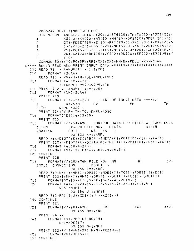
139
PROGRAM BENTl( INPUT,OLJTPUT) DIMENSION ANUM(20),DISTA(20),DISTB(20),THETA(20),POTT(20),
1 KS(20),KA(20),NN(20),HH(20),DPS(20),NDEI(20),TC( 2 20) ,FDBET(20) ,E(20) ,RRI (20,5) ,XX1I20,5) ,XX2(2C,5 3 ),ZZZ(5,25),SSS(5,25),NP(5,20),XS(5,20),YC(5,20, 4 25 ) ,PC ( 5,20,25) , I I ( 5) ,N C ( 5 ) ,F J Y ( 20) ,F JM ( 20) ,F JX ( 5 20),AA(2u),BB(20),CC(2u),DD(20),EE(2G),ES(lJ5),Y 6 (105)
COMMON ES,Y,YC,PC,DPS,RRI,XXl,XX2,HH,NN,FDBET,XS,NC,NP C**** BEGIN READ AND PRINT INPUT DATA ***************************
IJJ READ 71L , (ANUM(I) , 1=1,20) FORMAT (?CJA4)
READ 711 , PV,PH,TM,TOL,KNPL,KOSC 711 FORMAT (4EIC.4,2I5)
IF(KNPL) 9999,9999,110 lln PRINT 712, (ANUM(IhI=1,2C) 712 FOR~AT (lHl,20A4)
PRINT 713 713 FORMAT ( 11,5X,27H
1 4X,67H 2 TOL KNPL KOSC )
PV LIST OF INPUT DATA ---III
PH
PRINT 714,PV,PH,TM,TOL,KNPL,KOSC 714 FOR~AT(4E15.4,I3,I5)
PRINT 715
TM
71 5 FOR~~A T (11,5X,43H CONTROL DATA FOR PILES AT EACH LOCA
716 717 120
718
719 720
150
721
]TION 2BATTER
5X,80H PILE NO. DISTA DISTB POTT KS KA )
DO 120 K=l,KNPL READ 7]6,DISTA(K),DISTB(K),THETA(K),POTT(K),KS(K),KA(K) PRINT 717,K,DISTA(K),DIST8(K),THETA(K),POTT(K),KS(K),KA(K)
FORMAT (4EI0.4,2I5) FORMAT (5X,I5,lE15.4,3E12.4,I5,I4)
CONTINUE PRINT 718
FORMAT(II,10X,76H PILE NO. NN HH INDEI CONNECTION FDBET)
[10 150 I=l,KNPL READ 719,NN( I) ,HH( I) ,DPS( I) ,NDEI (I) ,TC( I) ,FDBET( I) ,E( I) PRINT 720,I,NN(I),HH(I ),DPS(I),NDEI( I),Te(I ),FDBET( I)
FOR~AT(5X,I5,2EIU.5,5X'I5,7X,A3,2EI0.5)
FORMAT (4X'I~,2X'I5,2EI5.5'I5,7X,A3,3X,EI5.5
NDST=NDEI(I) DO 15U J=l,NDST
READ 711,RRI(I,J),XXlII,J),XX2(I,J) COiH I NUE PRINT 721
FORMAT(II,20X,43H RRI DO 155 M=I,KNPL
PRINT 741,M
XXI
DPS
XX2)
741 FORMAT (5X,7HPILE NO,I5) NEI=NDEI(M)
DO 155 N=l,NtI PRINT 722,RRI (M,N) ,XXI (M,N) ,XX2(M,N)
722 FORMAT(20X,3E15.5) 155 CONTINUE

14·0
REAO 723,NKA,NKS,KOK PRINT 724
723 FORMATf3C5X,I5)) 724 FORMATCIII,9X,28H AXIAL LOAD SETTLEMENT DATA '"
DO 160 L=l,NKA READ 723,IDEN,IO PRINT 725,IDEN
72~ FORMATe9X,12H IOENTIFIER.I~,26H ZZZ SSS) IIfIDEN)=IO
DO 1 60 L L = 1 , I 0 READ 711,ZZZfIDEN,LL',SSSfIDEN,LL)
160 PRINT 726,ZZZeIDEN,LL),SSSfIDEN.LL) 726 FORMATC26X.2E15.5)
IFCKOK)126,126,151 126 PRINT 727 727 FORMATfll.9X,15H P-Y CURVES II)
DO 130 K=I,NKS READ 723.IDPY,KNC PRINT 728,IDPY,KNC
72A FORMATf9X,15H S~T IDENTIFIER 15,18H NO. CURVES IN SET 1I~"/)
NCCIDPY)=KNC DO 1"30 I=I.KNC
READ 719.NPf JC)Py, I )'XS( IDPY.r) PRINT 729
729 FORMATCII,9X.30H CURVE NP XS PRINT 730.I.NPfIDPY,I,.XSfIDPy.I)
730 FORMATf12X.I5,4X.I5,EI5.5) NT=NPCIDPY,Il
PRINT 731 7~1 FORMATfll,15x.20H YC PC
DO 130 L=I.NT RFAf) 711,YCfIOPY,I,L).PCCIDPY.I,L) PRINT 732,YCfIDPY,I.L),PCCIDPY,I,L)
732 FORMATC7X,2EI5.5) 130 CONTINUE
GO TO 152 c**** SUBROUTINE MAKE GENERATES P-Y CURVES FROM SOIL PROPERTIES *
151 CALL MAKEfNP,NC,yC,PC,XS) 152 CONTINUE
C**** SET INDICIES FOR INITIAL FJY,FJx.AND FJM ESTIMATION ******* 300 KFLAG=O
7"33 1
KEY=O KSW=0 ITER=O DV=O.O DH=O.O ALPHA=O.O
PRINT 733 FORMAT(/.35Hl 9X.45H DV
GO TO 325 310 CONTINUE
I TER= ITER+l
DH ITERATION DATA
ALPHA
(**** (HECK FOR DV,OH,ANO ALPHA CLOSURE *************************
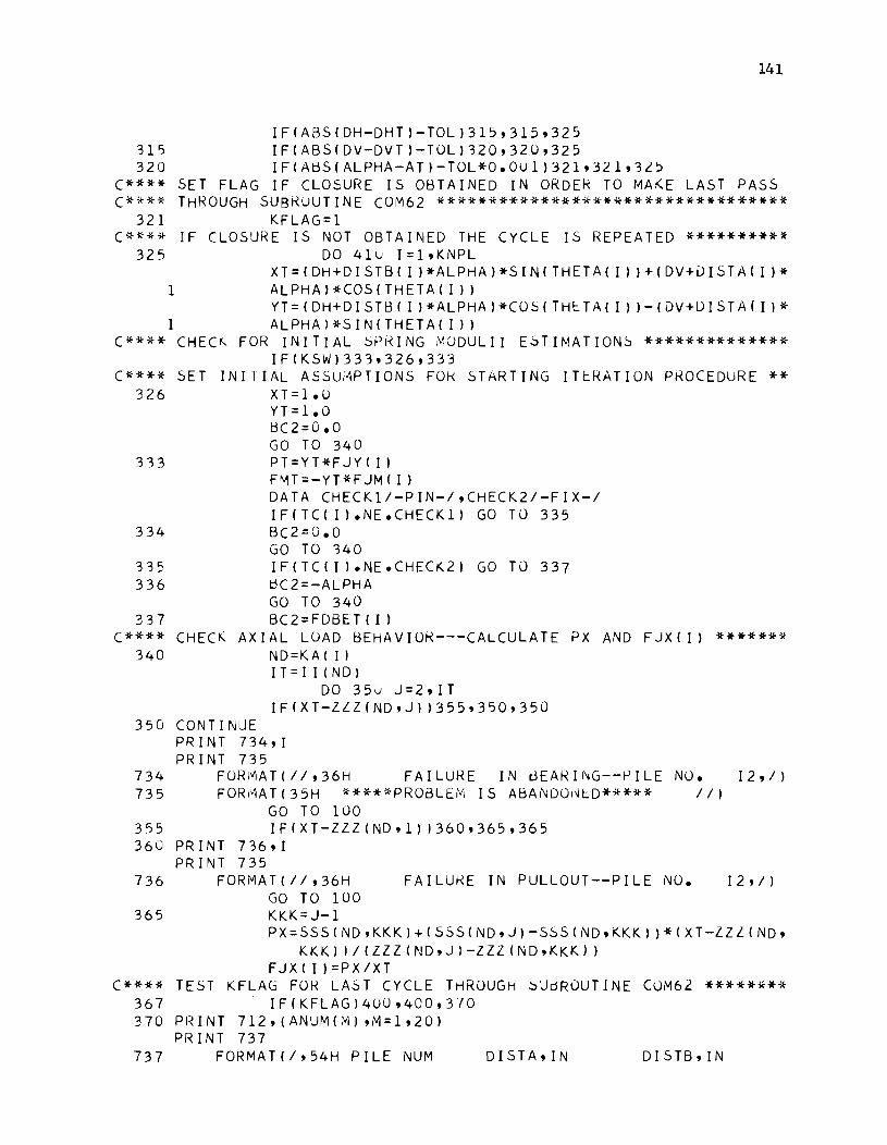
315 320
C**** C****
321 C****
325
1
1 C****
C**** 326
333
IF(ABS(DH-DHT)-TOL)315,315,325 IF(ABS(DV-DVT)-TOL)320,320,325 IF(ABS(ALPHA-AT)-TOL*0.OUl)321,321,325
141
SET FLAG IF CLOSURE IS OBTAINED IN ORDER TO MA(E LAST PASS THROUGH SUBRuUTINE COM62 **********************************
KFLAG=l IF CLOSURE IS NOT OBTAINED THE CYCLE IS REPEATED **********
DO 410 1=1,KNPL XT=(DH+DISTB( I )*ALPHA)*SIN(THETA(I I )+(DV+DISTA(I)* ALPHA)*COS(THETA(I )) YT=(DH+DISTB( I)*ALPHA)*COS(THETA(I) )-(OV+DISTA(I)* ALPHA)*SIN(THETA(II)
CHEC~ FOR INITIAL ~PRING MODULII ESTIMATIONS ************** IF(KSW)333,326,333
SET INITIAL ASSU~PTIONS FOR STARTING IT~RATION PROCEDURE ** XT=l.O YT=l.O BC2=0.0 GO TO 340 PT=YT*FJY(I) F~T=-YT*FJM(I)
DATA CHECK1/-PIN-I,CHECK21-FIX-I I F ( T C ( I ) • N E • C H E C K 1 1 GO TO 335
334 BC2=0.0 GO TO 340
335 IF!TC(II.NE.CHECK2) GO TO 337 336 ~C2=-ALPHA
GO TO 340 337 BC2=FDBET(I)
C**** CHECK AXIAL LOAD BEHAVIOk---CALCULATE PX AND FJX(I) ******* 340 ND=KA ( I 1
IT=II(ND) DO 350 J=2dT
IF(XT-ZZZ(NDd) )35593509350 350 CONTINUE
PRINT 73491 PRINT 735
734 FORMAT(II,36H FAILURE IN aEARI~G--PILE NO. 12,/1 735 FORI"1A T ( 35H *****PROBLEfVi I S ABAi\iOOI~tD***** III
GO TO 100 355 IF(XT-ZZZ(NDdI13609365,365 360 PRINT 736,1
736
365
PRINT 735 FORMA T ( II d6H
GO TO 100 FAILURE IN PULLOUT--PILE NO.
KKK=J-l PX=SSS(ND,KKKI+(SSS(ND,J)-SSS(ND,KKK))*(XT-lZZ(ND,
KKK) I/(ZZZ(ND,JI-ZZZ(ND,KKK)) FJX( I )=PX/XT
KFLAG FOR LAST CYCLE THROUGH ~UdROUTINE COM62 ******** C**** TEST 367 IF(KFLAGI40U,400,370
PRINT 712,(ANUM(:VI) ,M=1,20) PRINT 737
370
737 FORMAT(/,54H PILE NUM DISTA, IN DISTB, IN
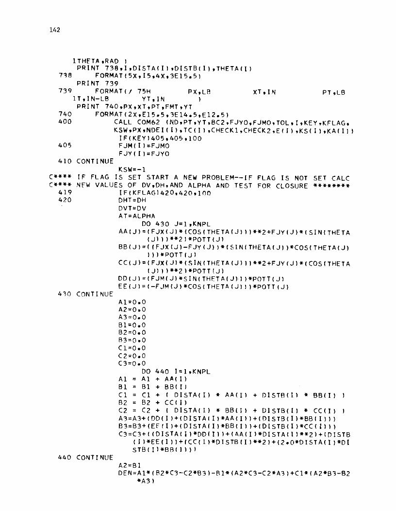
142
ITHE'TA,RAD ) PRINT 738,1 ,DISTA( I) ,DISTB( I) ,THETA(I)
7~8 FORMAT(Sx,IS,4X,3E1S.51 PRINT 739
739 FORMAT(I 7SH PX,LB XT,IN PT,LB IT,IN-LB YT,IN I
PRINT 740,PX,XT,PT,FMT,YT 740 FORMAT(2X,E1S.S,3EI4.5,EI2.S1 400 CALL COM62 (ND,PT,YT,BC2,FJYO,FJMO,TOL,I,KEY,KFLAG,
KSW,PX,NDEI (I) ,TC( I I ,CHECK1,CHECK2.E( I) ,KS( I) ,KA( I II IF(KEY140S,40S,100
405 FJM(I)=FJMO FJY( I )=FJYO
410 CONTINUE KSW=-1
C**** c****
419 420
IF FLAG IS SET START A NEW PROBLEM--IF FLAG IS NOT SET CALC NfW VALUES OF DV,DH,AND ALPHA AND TEST FOR CLOSURE ********
IF(KFLAGI420,420,100
410 CONTINUE
440 CONTINUE
DHT::DH DVT=DV AT=ALPHA
DO 430 J=I,KNPL AA(J)=(FJX(J)*(COS(THETA(J»)**2+FJY(JI*(SIN(THETA
(J» )**2)*POTTIJ) BB(J)=( (FJX(J)-FJY(J»*ISIN(THETA(J) )*COS(THETAIJ)
))*POTT(Jl CC(J)=(FJXIJ)*ISINITHETAIJ»)**2+FJY(J)*(COS(THETA
(Jl»**21*POTTfJ) DD(JI=IFJM(Jl*SIN(THETAIJ»l*POTT(J) EEIJ1=(-FJM(J)*COS(THETA(J»)*POTT(J)
Al=O.O A2==0.0 A3=0.0 Bl==O.O B2=0.0 B3=0.0 C1=0.0 C2=0.0 C3=0.0
DO 440 I=I,KNPL A1=Al+AA(IJ B1 ::; B1 + BB(II C1 = C1 + ( DISTA(l) * AA(I) + DISTBCI) * BB( 1) B2 = B2 + CCII) C2 :: C2 + ( DISTA(l) * BBII) + DlsTB(I) * ccn) A 3 = A 3 + ( DD ( I ) + ( DIS T A ( I ) * A A ( 1 ) ) +( DIS T B ( I ) * BB ( I ) I ) B 3= B 3+ ( E E ( I ) + ( DIS T A ( I ) *BB ( I ) ) + ( 0 I S TB ( I ) *CC ( I ) ) ) C3=C3+(IDISTA(I)*DD{I»+IAAII)*DISTA(I)**2)+(DISTB
( I ) *EE ( I ) ) + (CC ( I ) *D I S TB ( I ) **2) + (2. O*D 1ST A ( I ) *D I S T B ( I ) *B B ( I ) ) }
A2=Bl DEN=A1*(B2*C3-C2*B3)-Bl*(A2*C3-C2*A3)+Cl*(A2*B3-B2
*A3)

143
ALPHA=(A1*(B2*lM-PH*B3)-B1*(A2*lM-PH*A3)+PV*(A2*B3 -B2*A 3) ) IDEN
DV=(PV*(B2*C3-C2*B3)-B1*(PH*C3-C2*TM)+C1*(PH*B3-B2 *TM»/DEN
DH=(A1*(PH*C3-C2*TM)-PV*(A2*C3-C2*A3)+C1*(A2*TM-PH *A3»/DEN
PRINT 780,DV,DH,ALPHA 780 FORMAT(13X,3E15.4,/)
c**** TEST FOR OSCILLATING SOLUTION CONTROL ********************* IF(KOSC)310,310,445
C C C
445 IF(ITER-5)310,310,450 450 DV=0.5*(DV+DVT)
DH=0.5*(DH+DHT) ALPHA=0.5*(ALPHA+AT) GO TO 310
9999 CONTINUE END
SUBROUTINE COM62 (ND,PT,YT,BC2,FJYO,FJMO,TOL,ITYPE,KEY,KFLAG 1,KSW,PX,NDEI,TC,CHECK1,CHECK2,E,KS,KA)
DIMENSION Y(105),ES(105),XS(5,20),NC(5),NP(5,20),HH(20),NN 1 (20),DPS(20),RRI(20,5),XX1(20,5),XX2(20,5),A(105) 2 ,B(105),C(105),FDBET(20),R(105),BMT(4),YC(5,20,25) 3 ,PC(5,20,25)
COMMON ES,Y,YC,PC,DPS,RRI,XX1,XX2,HH,NN,FDBET,XS,NC,NP C**** SET INDICIES AND OTHER CONSTANTS **************************
H=HH(ITYPE) N=NN( ITYPE) NP3=N+3 ITER=l K=l
c**** CAL. INITIAL ES VALUES (ES=KX,K=1.0) AND EI=R DISTRIBUTION c**** ALONG THE PILE (STATION 3 IS TOP OF PILE) *****************
1025
1030 1035 1040
DO 1051 J=3,NP3 Y(J)=O.O lJ=J-3 IF(DPS(ITYPE)-ZJ*H)1030,1030,1025 ES(J)=O.O GO TO 1035 ES(J)=1.0*lJ*H-DPS(ITYPE) IF(XX2(ITYPE,K)-lJ*H)1040,1050,1050 K=K+1 IF(K-NDEI)1035,1035,1045
1045 PRINT 1015,ITYPE PRINT 1017
1015 1LE
1017
FORMAT(II 61H EI DISTRIBUTION DOES NOT COVER TOTAL PI LENGTH--PILE NO 15)
FORMAT(II 30H ***PROBLEM IS ABANDONED***** I) KEY=l
RETURN 1050 R(J)=RRI(ITYPE,K) 1051 CONTI NUE
c**** CALCULATE A AND B COEFFICIENTS FOR PILE

144
1052
1
1
1 2
1
1 2
1 2
N2=NP3-1 Nl=NP3-2 A(NP3'=(4.0·R(N2'-2.0*PX*H**2,/(2.0*R(N2'-2.0*PX*H
**2+ES(NP3'*H**4, B(NP3'=(2.0*R(N2,}/(2.0*R(N2,-2.0*PX*H**2+ES(NP3'*
H**4' A(N2)=(2.0*R(Nl)+(2.0*R(N2,-PX*H**2,*(1.0-B(NP3" )
I(R(Nl'+(2.0*R(N2,-PX*H**2)*(2.0-A(NP3, )+ES( N2'*H**4'
B(N2,=R(Nl)/(R(Nl'+(2.0*R(N2)-PX*H**2)*(2.0-A(NP3' ,+ES(N2,*H**4,
DO 1080 J=4,Nl KT=NP3-J+2 C(KT,=R(KT-l'+R(KT'*(4.0-2.0*A(KT+l, '+R(KT+l,*(A(K
T+l'*A(KT+2'-~(KT+2)-2.0*A(KT+l'+1.0)-PX*H**
2*(2.u-A(KT+l' '+ES(KT,*H**4 A(KT'=(2.U*R(KT-l'+R(KT)*(2.0-2.0*B(KT+l, )+R(KT+l)
*(A(KT+2)*B(KT+l)-2.0*B(KT+l) ,-PX*H**2*(1.0-B(KT+l" )/C(KT'
B(KT)=R(KT-l)/C(KT' lUIF' CONTINUE
1054 lU55 1056 lu57
C**** USE lU65
C**** LJSE lU66
YTMPl=Y(3' YTMP2=Y(4) IF(TC.NE.CHECKl) GO TO 1055 IF(KSW)1070,1065,1065 IF(TC.NE.CHECK2' GO TO lU57 IF(KSW)1071,1066,1~66
IF(KSW)1072,1067,1067 BC2=YT FOR FIRST PASS (PINNED CONNECTION, *************
Y(3,=YT Y(4,=YT*( (A(4'-2.U*S(4),f( 1.0-6(4')' GO TO 1081
BC2=YT FOR FIRST PASS (FIXED CONNECTION) ************** S4=2.0*H*I3C2 Y(3'=YT Y(4)=(A(4)*YT+B(4,*S4,/(1.0+B(4)' GO TO 1081
C**** USE BC2=YT FUR FIk~T PASS (KESTkAINED CUNNECTIuN,********** Iv67 S5=BC2*(H/2*R(3' ,
Y(3,=YT Y(4,=(YT*(A(4)+A(4,*S5-2.U*B(4) ),/(1.0+S5+B(4)*S5-
1 B (4) ,
GO TO 1081 c**** CALCULATION OF Y3 AND Y4 wITH BCl=PT ANU 6C2=MT ***********
1070
C**** 1071
1 2 3
S,=2.U*PT*H**3 Gl=2.0-A(4' G2=1.0-B(4' Y(3,=S3*G2/(Gl*(R(3,*(2.0*B(4)-2.0)+R(4'*(4.0*13(4)
-2.0*A(5)*B(4, )-2.0*PX*H**2*B(4))+G2*(R(3'*(4 .O-2.0*A(4))+R(4)*(2.0*A*4,*A(5)-2.0*6(5)-4.0 *A(4)+2.0,+PX*H**2*(-2.0+2.0*A(4) ,+ES(3,*H**4,)
Y(4,=Y(3'*(A(4)-13(4)*GI/G2' GO TO 1081
CALCULATION OF Y3 AND Y4 WITH 6Cl=PT ANu 6C2=5T *********** S3=2.U*PT*H**3
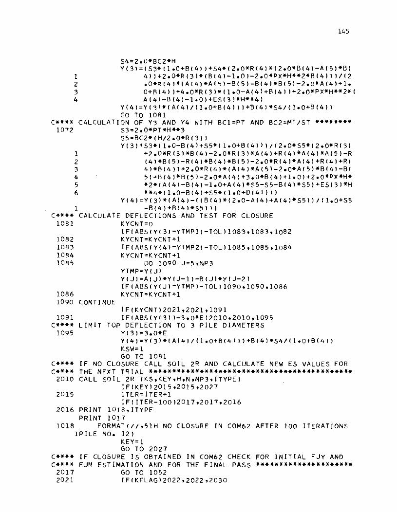
C**** 1072
C**** 1081
1082 1083 1084 1085
1086
1 2 3 4
1 2 3 4 5 6
145
S4=2.U*BC2*H Y(3)=CS3*C1.0+BC4) )+S4*C2.0*RC4)*C2.0*BC4)-AC5)*BC
4»+2.0*RC31*CBC4)-1.0)-2.0*PX*H**2*BC4» )/C2 .0*R(4)*CAC4)*AC5)-BC5)-BC4)*BC5)-2.0*AC4)+1. 0+B(4) )+4.0*RC3)*C1.0-AC4)+BC4»+2.0*PX*H**2*C A(4)-BC4)-1.0)+ESC3)*H**4)
Y(4)=YC3)*CAC4)/C1.0+BC4»)+BC4)*S4/C1.0+BC4» GO TO lOBI
CALCULATION OF Y3 AND Y4 WITH BC1=PT AND BC2=MT/ST ******** S3=2.0*PT*H**3 S5=BC2*CH/2.0*R(3» YC3l·S3*C1.0-B(4)+S5*C1.0+BC4»)/C2.0*S5*C2.0*RC3)
+2.0*R(3)*BC4)-2.0*RC3)*AC4)+RC4)*AC4)*AC5)-R (4)*BC5)-RC4)*BC4)*BC5)-2.0*RC4)*AC4)+RC4)+RC 4)*BC4»+2.0*RC4)*CAC4)*AC5)-2.0*AC5)*BC4)-BC 5)+BC4)*BC5)-2.0*AC4)+3.0*BC4)+1.0)+2.0*PX*H* *2*CA(4)-BC4)-1.0+AC4)*S5-S5-BC4)*S5)+ES(3)*H **4*C1.0-8(4)+S5*C1.0+BC4») )
Y(4)=YC3)*CAC4)-CCBC4)*C2.0-AC4)+AC4)*S5»/C1.0+S5 1 -B(4)+BC4)*S5)')
CALCULATE DEFLECTIONS AND TEST FOR CLOSURE KYCNT=O IFCABSCY(3)-YTMP1)-TOL)1083,1083,1082 KYCNT=KYCNT+l IFCABSCYC4,-YTMP2)-TOL)1085,1085,1084 KYCNT=KYCNT+1
DO 1090 J=5,NP3 YTMP=YCJ) YCJ)=ACJ)*YCJ-1)-BCJ)*YCJ-2) IFCABSCYCJ,-YTMP)-TOL)1090,1090,1086 KYCNT=KYCNT+1
1090 CONTINUE IFCKYCNT)2021,2021,1091 IFCABSCY(3) )-3.0*E)2010,2010,1095
C**** LIMIT TOP DEFLECTION TO 3 PILE DIAMETERS 1091
1095 Y(3)=3.0*E Y(4)=YC3)*CAC4'/C1.0+BC4) »+BC4)*S4/C1.0+8C4» KSW=l GO TO lOBI
c**** IF NO CLOSURE CALL SOIL 2R AND CALCULATE NEW ES VALUES FOR C**** THE NEXT TRIAL ********************************************
2010 CALL SOIL 2R CKS,KEY,H,N,NP3,ITYPE)
2015 IFCKEY)2015,2015,2027 ITER=ITER+1 IFCITER-100)2017,2017,2016
2016 PRINT 1018,ITYPE PRINT 1017
1018 FORMATCII,51H NO CLOSURE IN COM62 AFTER 100 ITERATIONS 1 P I L E NO. 12)
KEY=l GO TO 2027
c**** IF CLOSURE IS OBTAINED IN COM62 CHECK FOR INITIAL FJy AND C****
2017 2021
FJM ESTIMATION AND FOR THE FINAL PASS ********************* GO TO 1052 IFCKFLAG)2022,2022,2030

146
2,-,22 2,-,24
1 2 3 4
2 ~\ 25 2v28
1
IFIKSW)2u25,2024,2024 PT=11.0/12.U*H**3) )*IYI5)*RI4)+YI4)*IRI4)*IAI5)-4.
U)+2.0*PX*H**2/BI4)+2.0*RI31*11.0/BI4)-1.0) )+YI 3)*IRI4)*12.0-BI5) )+PX*H**2*1-2.0*AI4)/BI4)+2 .0*A(4)-2.0)+RI3)*14.0-2.0*AI4)/BI4) )+ESI3)*H **4) )
IFITC.NE.CHECK1) GO TO 2029 FJMO=O.O FJYO=PT/Y(3) GO TO 2031 FJYO=PT/Y(3) TMOM=IR(3)/H**2)*IYI3)*IAI4)/~14)-2.0)+YI4)*1 1.0-1
.0/B(4)) ) FJMO=-TMOM/Y(3)
2",1 IFIKSW)2027,2027,2026 2U26 KS~=-l
2u27 RETURN C**** IF THE FLAG IS SET CALCULATE MOMENT AND SOIL RESISTANCE C**** ALONG THE PILE,PKINT RESULTS,ANU RETURN TU MAIN PRUGRAM ***
2030 PRINT 1002 PRINT 1U03
1u02 FORMAT 15X,18H INPUT INFURMATIUN I) 1003 FORMATI5X,78H PT,LB PX,LB TC TOP
1UIA,IN INC. L~NGTH,IN NO.OF INC I) 2w41 PRINT 1v10,TC,E,H,N,KS,KA lv10 FORMATI9X,A3,2E15.4,3X,I~,'X,2I')
PRINT 1U04 1~U4 FORMAT(/,5X,71H PILE LENGTH,IN DEPTH TO SOIL ITERATION
1 TOL. BOUNDRY COND.2 KS KA I) ZN=N PLGTH=ZN*H
PRINT 101l,PLGTH,DPSIITYPE),TOL,BC2 1011 FORMATI5X,4E15.4)
PRINT 1u06 1~U6 FOkMATI/,3uX,19H OUTPuT INFURMATIUN I)
c**** TEST FOR INVALID SOLUTION IFIKSW)2047,2046,2U46
2046 PRINT lUl9 1~19 FORMATII 82H INVALID ~OLUTION ~INCE EXCESSIVE DEFLECTION
1 CONTROL ESTABLISHED DURING THIS CYCLE II) 2U47 PRINT 1007 1u07 FORMATI5X,75H X,IN Y,IN MOMENT,IN
1-LB ES,LR/IN2 P,LB/IN I) NP4=NP3+1 YINP4)=U.0 Y(2)=IAI4)*YI3)-YI4))/~14)
DO 2050 J=3,NP3 FMO=RIJ)*IYIJ-1)-2.0*YIJ)+YIJ+1))/IH*H) RES=-ESIJ)*Y(J) ZJ=J-3 XIN=ZJ*H
PRINT 1013,XIN,YIJ),FMO,ES(J),RES 1013 FORMAT(5X,5E13.5) 2U50 CONTINUE
RETURN

C C C
3010
147
END
SUBROUTINE SOIL 2R (KS,KEY,H,N,NP3,ITYPE) DIMENSION Y(105),ES(105),PC(5,20,25),YC(5,20,25),NC(5),XS(5
1 ,20),EST(20),DPS(20),RRI(20,5),XX1(20,5),XX2(20,5 2 ),NN(20),FDBET(20),NP{5,20)HH(20)
COMMON ES,Y,YC,PC,DPS,RRI,XX1,XX2,HH,NN,FDBET,XS,NC,NP K=2
DO 3090 J=3,NP3 ZJ=J-3 Z=ZJ*H-DPS(ITYPE) IF(Z)3010,3015,3015 ES(J)=O.O GO TO 3090
C**** LOCATE 3015
P-Y CURVES ABOVE AND BELOW GiVEN IF(XS(KS,K)-Z)3020,3027,3030 K=K+1
DEPTH
3020 IF(K-NC(KS) )3015,3015,3025
3025 PRINT 3000 PRINT 3001
3000 FORMAT( II 52H P-Y CURVES DO NOT EXTEND THE LENGTH 10F THE PILE )
3001 FORMAT( I 35H KEY=l
3026 RETURN
*****PROBLEM IS A8ANDONED***** I )
3027 M=K GO TO 3035
3030 M=K-1 3035 YA=ABS(Y(J»
IF(YA-1.0E-10)3036,3037,3037 3036 YA=1.0E-10
C**** LOCATE POINTS BEHIND AND AHEAD OF YA ON EACH P-Y CURVE AND C**** COMPUTE ES ON EACH CURVE BY LINEAR INTERPOLATION **********
3037 DO 3070 I=M,K
3040 3045
3050
3055
3060 1
3065 3070
C****
3075
3080 1
CONTINUE
L=2 IF(YC(KS,I,L)-YA)3045,3055,3060 L=L+1 IF(L-NP(KS,I»3040,3040,3050 P1=PC(Ks,I,L-1) GO TO 3065 P1=PC(Ks,I,l) GO TO 3065 PI = P C ( K S , I , U - ( PC ( K S , I , L ) - PC ( K S , I , L -1 ) ) * ( Y C ( K S , I , L
)-YA)/(YC(KS,I,L)-YC(KS,I,L-1» EST( I )=P1/YA
INTERPOLATE BETWEEN CURVES FOR CORRECT ES VALUE IF(K-M)3075,3075,3080 ES(J)=EST(K) GO TO 3090 ES(J)=(EST(K)-(EST(K)-EST(M»*(XS(KS,K)-Z)/(XS(KS,
K)-XS(KS,M») 3090 CONTINUE

~8
RETURN END
SUBROUTINE MAKE (IPOINT,NC,YC,P(,OTCI DIMENSION TSOILllul,GAMMA(10),PHII10),UISI(10),DIS2(10),KDE
1 NSE(10),FKO(10),AV(I~),~HEAR~II0)'INFO{10)'ICON(1
2 O),NCURVS{10),DIST(IJ,10).NPOINTII0,10),SIGD(10,1 3 O'15),FP(10'10'151'D(5),DI~Dl{5),DISD2{5),DTC(5,2 4 O),PCI5,20,25),YC(5,20,25),IPOINT(5,201,QII0),NC( 5 51
10 FORMAT (5X,I5) 11 FORMAT (6X,A41 12 FORMAT (4EIO.4,5X,A41 13 FORMAT (4EI0.4,5X,I5,6X,A4) 14 FORMAT (EIU.4,5X,15) 15 FORMAT (2EI0.4) 16 FORMAT (5X,I5,5X,I5,5X,I5) 17 FORMAT (3EI0.41 18 FORMAT (EIU.4) 19 FORMAT(II,5X,26H INPUT OF SOIL PARAMETERS III) 20 FORMAT (5X,18H SOIL PROFILE NO. I5,16H STRATUM NO. 15,1
5H TYPE SOIL A4111 21 FORMAT { 75H UNIT WEIGHT
lOTTOM DEPTH DENSITY 22 FORMAT (4EI5.4,5X,A41 23 FORMAT ( 75H UNIT WEIGHT
10TTOM DEPTH CONSISTENCY 24 FORMAT I1X,4EI4.4,5X,A4,/) 25 FORMAT (5X,31H STRESS STRAIN 26 FORMAT (11H CURVE NO. 12,16H 27 FORMAT (25H STRESS 28 FORMAT 15X,EI0.4,5X,EI0.4) 29 FORMAT (IHl) 30 FORMAT (5X,36H
ANGLe OF FRIC. I I
COHESION I
TOP DEPTH
TOP DEPTH
CURVES FOR CLAYIII) DEPTH TO CURVE EI0.411) STRAIN III
P-Y CURVES I
B
31 FORMAT (20H SET IDENTIFIER NO. I5,30H NUMBER OF CURVES 1 IN SET 151/1)
32 FORMAT (11,15X,31H DIAMETER DISTRIBUTION FOR PILEI) 33 FORMAT (38H DIAMETER TOP DIS BOT DIS 34 FORMAT {IIX,EI0.4,5X,Elv.4,5X,EI0.4,111 35 FORMAT (11,IIH CURVE NO. I5,16H DEPTH TO CURVE EI0.4,/) 36 FORMAT (35H SOIL REACTION DEFLECTION I 37 FORMAT (EI5.4,5X,EI5.4)
C •••• READ INFURMATIUN FUR SOIL PRUFILES •••••••••••••••••••••••• PRINT 19 READ 10 , NSOILP DATA TESTl/-SAND-I,TEST2/-CLAY-I,IlE~TA/-DENS-I'ITESTB/-MEDM-I DATA ITESTC/-LOSE-I,ITESTX/-SOFT-I,ITESTZ/-STIF-I DO 553 ISP= 1 ,NSOILP READ 10 , NSTYPE DO 510 1ST = 1 , NSTYPE READ 11 , TSOIL(ISTI PRINT 2J , ISP,IST,TSOIL(IST) IF(TSOIL(ISTI.NE.TESTl) GO TO 507

149
~00 READ 12tGAMMA(IST),PHI(I~T)tDISl(I~T),UIS2(IST),KDENSE(IST)
PRINT 21 PRINT 22,GAMMA(IST),PHI(IST),DIS1(IST),DIS2(IST),KDENSE(IST) IFCKDENSE(IST).NE.ITESTAI GO TO 502
501 FKOCIST)=O.4U AV(IST) =1500.0 GO TO 510
502 IF(KDENSECIST).NE.ITESTB) GO TO 504 503 FKO(IST)=0.45
A.V(ISl) = 6UO.0 GO TO 510
504 FKOCIST)=0.50 AV(IST) =200.0 GO TO 510
5a7 READ 13,GAMMAC 1ST) ,SHEARS( 1ST) tDI~lf 1ST) ,OIS2( 1ST), INFO( 1ST) 1,ICON(IST)
PRINT 23 PR IN T 24, GAMMA CIS T ) ,SH EAR ( 1ST) ,0 I ~ 1 ( 1ST) ,0 I S2 ( 1ST) I CON ( 1ST) IF( INFO( 1ST)) 510,510,508
508 READ 10 , NCURVSIISTI PRINT 25 NCUR= NCURVS(IST) DO 509 JJ=l,NCUR READ 14 , DISTII~T,JJ), NPOINTIIST,JJ) PRINT 26 , JJ, OIST( IST,JJ) PRINT 27 NPZ = NPOINT( IST,JJ) DO 509 JK=l,NPZ READ 15, SIGO( IST,JJ,JK) ,FP( IST,JJ,JK) PRINT 28 , SIGDIIST,JJ,JK) ,FPIIST,JJ,JKI
5U9 CONTINUE 51() CONTINUE
C**** READ PILE DATA FuR USE IN GENERATION OF P-Y CURVRS ******** READ 10 , NPISP 00 553 JP= 1 , NPISP PRINT 29 PRINT 30 READ 16 , KS , NOC , NDD
NC(KS)=NOC PRINT 32 PRINT 33 DO 511 JO= 1,NDD READ 17 , O(JO) , OISOllJO) , DIS02(JD)
511 PRINT 34, 0(JO),OISOl(JO),OISD2(JO) PRINT 3ltKS,NOC DO 553 IJK= I,NOC READ 18 , OTC(KS,IJK) PRINT 35, IJK , OTC(KS,IJK) PRINT 36 DO 512 IFS= I,NSTYPE IF(OIS2IIFS)-OTC(KS,IJK)) 512,513,513
512 CONTINUE 513 IF(TSOILIIFS).NE.TESTI) GO TO 528
C**** GENERATION OF p-y CURVES IN SAND ************************** 514 IF( IFS-ll 517 , 517 , 515

150
515 SWGA~= 0.0 SDIS = 0.0 DO 516111= 1,I.FS WGAM = GAMMAI III )*(DIS21 III )-DISlI III)) SWGAM =SWGAM + WGAM
516 SDIS = SDIS + IDIS2(111)-DISIIIIII1 AGA~ = SWGAM/SDIS GO TO 518
517 AGAM = GAMMAIIFS) 518 DO 519 IPT= I,NDD
IFIDISD21 IPT)-DTCIKS,IJK)) 519 , 520 , 520 519 CONTINUE 520 DIA= DIIPT)
ALPHA= PHIIIFS)/2.0 ES= IAVIIFS)*AGAM*DTCIKS,IJK))/1.35 IFIES) 596,596,595
596 PCIKS,IJK,2)=0.O YCIKS,IJK,2)=1.0 GO TO 597
595 C2=COSIALPHA) C3= TANIPHIIIFS)) C4= TANIALPHA) C5= TANIO.78539+PHIIIFS)/2.0) C6=C5**2 C7= SINIO.78539+PHIIIFS)/2.0) C8= TANIO.78539-PHIIIFS)/2.0) C9= C8**2 Al= AGAM*DIA*IC5/C8-(9) A2= AGAM*IC6*C4/C8+FKOIIFS)*C7*C3/IC2*C8)+FKOIIFS)*C5*C3*C7
1 -FKOIIFS)*C5*C4) A3= AGAM*C9*DIA*IC6**4-1.U)+FKOIIFS)*DIA*AGAM*C3*C6**2 PUW= Al*DTCIKS,IJK)+A2*DTCIKS,IJK)**2 PUF= A3*DTCIKS,IJK) IFIPUW-PUF)525,526,526
525 PCIKS,IJK,2) = PUW GO TO 527
526 PCIKS,IJK,2) = PUF 527 YCIKS,IJK,2) = PCIKS,IJK,2)/ES 597 YCIKS,IJK,l)=O.O
PCIKS,IJK,I) = 0.0 YCIKS,IJK,3) = 10.0*DIA PCIKS,IJK,3) = PCIKS,IJK,2) IPOINTIKS,IJK) = 3 DO 560 LZ = 1,3
560 PRINT 37 , PCIKS,IJK,LZ) , YCIKS,IJK,LZ) GO TO 553
C**** GENERATION OF P-Y CURVES IN CLAy ************************** 528 IFIINFOIIFS)) 529,529,548
c**** GENERATION OF P-Y CURVES FOR CLAY W/O STRESS STRAIN CURVES C**** AVALIABLE *************************************************
529 IFIICONIIFS).NE.ITESTX) GO TO 531 530 EP50=C.02
GO TO 534 531 IFI ICONI IFS).NE.ITESTZ) GO TO 533 532 EP50=O.005

GO TO 534 533 EP50=0.Ol 534 IF(IFS-ll 535,535,536 535 AGAM=GAMMA(IFS)
GO TO 538 536 SGAM=O.U
SDIS=O.O DO 537 III=l,IFS GAM= GAMMA(III)*(DIS2( III )-DIS1(III)) SGAM= SGAM+GAM SDIS= SDIS+(DIS2(III )-DIS1(III))
537 CONTINUE AGAM= SGAM/SDIS
538 DO 539 IPT= 1,NDD IF(DISD2( IPT)-DTC(KS,IJK) )539,540,540
539 CONTINUE 540 DIA= D(IPT)
151
PUW= AGAM*DIA*DTC(KS,IJK)+2.0*SHEARS(IFS)*DIA+2.S3*SHEARS(I 1 FS)*DTC(KS,IJK)
PUF= 11.0*SHEARS(IFS)*DIA SIG50= SHEARS( IFS) A= 2.0*(ALOG10(2.0))+ALOG10(EP501 EP100= 10.0**A DIFF = EP10U/10.U IF(PUF-PUW) 541,541,542
541 MPOINT = 12 P((KS,IJK,12) = PUF PC(KS,IJKtl1) = PUF YC(KS,IJK,121 = 10.O*DIA YC(KS,IJK,ll) = EP100*DIA IPOINT(KS,IJK) = 12 GO TO 546
542 STUP = 9.0 DO 543 ITO=1,9 EP= STUP*DIFF STUP= STUP-l.O PSD= ALOGIO(SIG50)+O.5*(ALOGIO(EP)-ALOGIO(EP50))
SIGA= 10.0**PSD Q(ITO)= 5.S*SIGA*DIA I~(PUW-Q( ITO)) 543,544,545
543 CONTINUE UIFF=DIFF/IO.O STUP=9.0 DO 561 ITO=1,9 EP=STUP*DIFF STUP=STUP-l.ll PSQ=ALOGIO(SIG50)+O.5*(ALOGIO(EP)-ALOG10(EP50)) SIGA=10.0**PSD Q(IT01=5.S*SIGA*DIA IF(PUW-Q( ITO)) 56lt562,562
561 CONTINUE 562 IPOINT(KS,IJK)=3
rC(KS,IJK,3)=PUW YC(KS,IJK,3)=lO.O*DIA PC(KS,IJK,2)=PUW
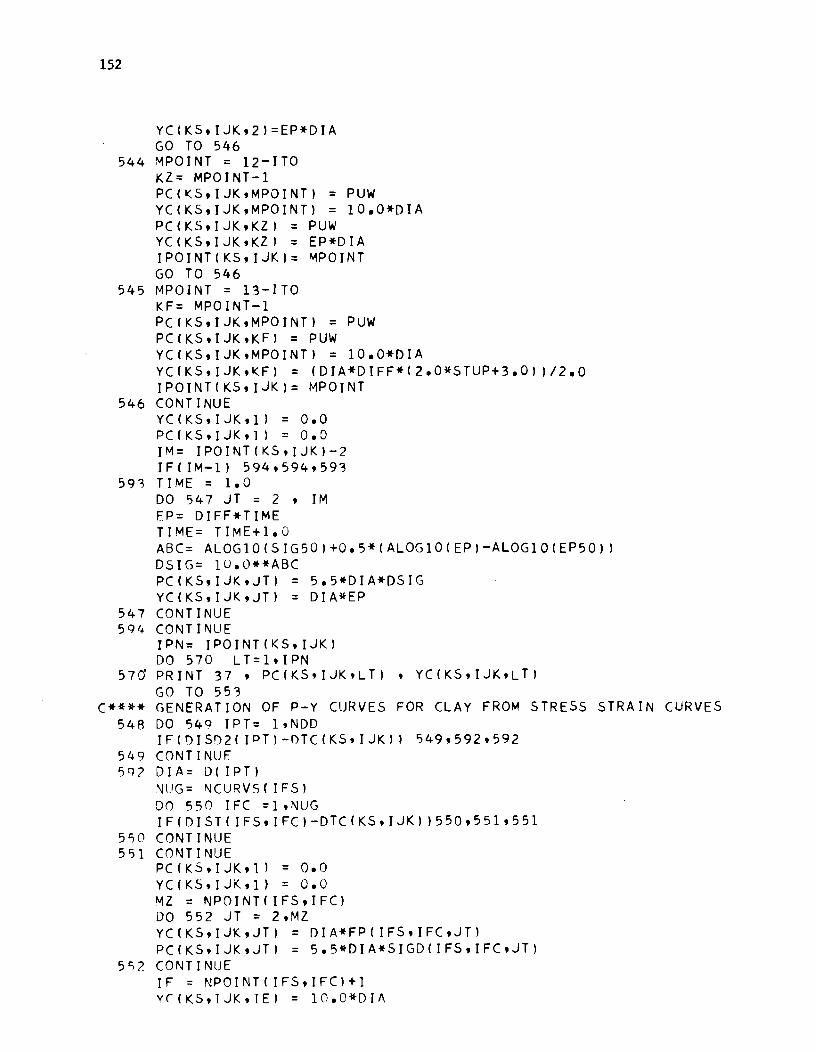
152
YC(KS,IJK,21=EP*DIA GO TO 546
544 MPOINT = 12-ITO KZ= MPOINT-l PC(KS,IJK,MPOINTI = PUW YC(KS,IJK,MPOINTI = 10.0*DIA PC(KS,IJK,KZI = PUW YC(KS,IJK,KZI = EP*DIA IPOINT(KS,IJKI= MPOINT GO TO 546
545 MPOINT = 13-ITO KF= MPOINT-l PC(KS,IJK,MPOINTI = PUW PC(KS,IJK,KFI = PUW YC(KS,IJK,MPOINTI = 10.0*DIA YC(KS,IJK,KFI = (DIA*DIFF*(2.0*STUP+3.011/2.0 IPOINT(KS,IJKI= MPOINT
546 CONTINUE YC(KS,IJK,ll = 0.0 PC(KS,IJK,1 I = 0.0 IM= IPOINT(KS,IJKI-2 IF( 1M-II 594,594,593
59~ TIME = 1.0 DO 547 JT = 2 , 1M EP= DIFF*TIME TIME= TIME+l.O ABC= ALOG10(SIG501+0.5*(ALOGlO(EPI-ALOGlO(EP501 I DSIG= lO.O**ABC PC(KS,IJK,JTI = 5.5*DIA*DSIG YC(KS,IJK,JTI = DIA*EP
547 CONTINUE 594 CONTINUE
yPN= IPOINT(KS,IJKI DO 570 LT=l,IPN
57cr PRINT 37 , PC(KS,IJK,LTI , YC(KS,IJK'LTI GO TO 553
C**** GENERATION OF P-Y CURVES FOR CLAY FROM STRESS STRAIN CURVES 548 DO 549 IPT= 1,NDD
IF(OISD2( IPT)-DTC(KStlJKII 549,592,592 549 CONTINUE 5q? DIA= D( IPTI
NUG= NCURVS(IFS) DO 550 IFC =l,NUG IF(DIST(IFS,IFCI-DTC(KS,IJKI1550,551,551
550 CONTINUE 551 CONTINUE
PC(KS,IJK,1) = 0.0 YC(KS,IJK,ll = 0.0 MZ = NPOINT(IFS,IFCI DO 552 JT = 2,MZ YC(KS,IJK,JTI = DIA*FP(IFS,IFC,JT) PC(KS,IJK,JTI = 5.5*DIA*SIGD(IFS,IFC,JT)
552 CONTINUE IE = NPOINT(IFS,IFC)+1 YC(KS,IJK,IEI = lO.O*DIA

IE] = IE-1 P((KS,IJK,IE) = P((KS,IJK,IEl) IPOINTIKS,IJKI = IE TPA= TPOINT(KS,YJKI DO 580 LX=l.IPB
5AC PRTNT 17 , P(IKS,IJK'LX) , Y(IKS,IJK.LX) 55":!, (O~TJNUE
RETURN END
153

!!!!!!!!!!!!!!!!!!!"#$%!&'()!*)&+',)%!'-!$-.)-.$/-'++0!1+'-2!&'()!$-!.#)!/*$($-'+3!
44!5"6!7$1*'*0!8$($.$9'.$/-!")':!
APPENDIX E
CODED INPUT FOR EXAMPLE PROBLEMS

!!!!!!!!!!!!!!!!!!!"#$%!&'()!*)&+',)%!'-!$-.)-.$/-'++0!1+'-2!&'()!$-!.#)!/*$($-'+3!
44!5"6!7$1*'*0!8$($.$9'.$/-!")':!

157
IDENTIFICATION LNPIJT" "F'>EIIIT 1 - £x'.I1MPLE L
I I I 2:0 25 30 3~ 40 4 ~o 5 &0 S~ 70 ,"0
Ii I.?I~ Ir +-l.-l -l< 14 v:IJv: , II) ;",I.lr i i II I I II i I
i
, >-,1. ,_ 1.1 j I. ,_,1 i I I, I I i I I, 1/ ,I ,~,I ,. "VlIF'T ' ,:r,{~hFl+- h ',: II, lJ:1rlx '1/ II
'rt l3 +1/l-'!r ,llvJJ: I) 1/1/~.bl~ iii I, II Iii I
: I;;: I [1, ~(~ hll) I, \?v'tl~:+-;"'9 i 'i II I 1'1 'I ,~~) I 1 'I !/ ,I~II iJ: 1/11
~: ;~, ~Efhl ~ i~d~t~h ill/. <I,J-f~'i i I I ,I i I ! I II : I ! ,i ! I : I I
I : i I I I I, 'I I , " 1:':1 II I, i' 'i I.; i " " I Ii I I Ii' I ' I, T I 11 i
'II \ ',I! il III I \ 'I', I/~ iii I, ! I 'I! 'i' , I \ I: I, I ill I I i i '0
IDENTIFICATION L/YPOT RENT1 - ffJ(RM?LE L
Z5 30 35 40 45 50 5 60 65 " , .0
II ~ IEf' I I i I I I
II ,
I \
,
,
rzls< IE+- I I Ii 'I ii"'! :1,1 ,i!1 iii! ill! li\'1 nl, Till , ii" I i I ! I
':1 i I i , - I~'( \I; IL ~blf' ~ i!! I I i I, \ !' II i I! II i! ! I' I, :! 'I i II: i I il 'I ,Iii
J v.v!f- - ~ ,14-~ hbi)",!£ \ II I, :. il i : I I I,! I '! I I i I I i I I I I,! III Ii I:,' ,
, II : 1'1 I
'+- v 'it1hIJ+ia~ II I I \ 'I I, I, !:!! ,', I I ' :. Ii I, Ii! I I I I, Ii:, ! i I :, I I I I ,
i I , , I IJ I I
': ,
! ! ~ : : i I I Iii I I
i
I i, :
I ! I ,
, , ,
I ! : ,
, I I , I i ' i
,
I II ! i
, "
,
I I , I
I i
i I Ii , ,
, I
~I.lsk ~_ki j~, !~! U.J II I, I I" il ! i ': : I I I II I '\ i ! I I I:' I ":: 'i I ,! ! .: : I ,i,'.' i I,
iii ;' i!: i I I
I ' ' ! I 'i I 1,1 I I I 'I i' I I "'I' , , i , /" IA iJ. ~i :6rlt.JJtlo II ; ! i i . I iii I Ii Ii! i ! I :, , ' I ! II ',: il I II! i I' i'l II
Ii' I', I, i
III I , I ii' I I III: I' IT I ! 'I . I I I I!., II I I I iii' Iii i I! : ill; , I: :: II I , I ! il I, II ii i I ! I I I I I',: I I, II' Ii, I 5 10 I ~ 20 25 30 35 40 45 50 5

158
IDENTIFICATiON .z;.pur 'BENT! -ExnMPL..E t CODED BY F P4-~Eg DATE 612// 6~ PAGL~OF~
I i, I I ,
lo ~ IFIT
i i II r I~ II I
i I, \ 11 I I
I
I;
I I , I'
'I I , I II I ~ II i I ; ,I., I j J I I I I 1 II ,II It: VJ'" 'It()~ . I-?v,v:\;; +!t:L2, I , :()' ,,' ,1"I! I Iii i I I, I I \ II , i i II i ! i I I I :
i 1
" " , 00
DENTIFICATION z: N'P()T CODED BY DATE . PAGE OF
, , ,0 , 20 " '0 " .0 " '0 , 60 ., 70 7 SO
~hl. jth~ I I I ,
I
~.~ kl-+hl I, , I I, I I
IC! ~ IFt"fl ! , I
II II I "
I I
I i II \ I I II
Ii I I i I 'I 11 I I I I
I I , ,
I
I ! i 1 ,
I Ii I, II I 'I I
'I i I II II' I I , ' I II j I ' 'I II 'I I Iii I I I I I 11 i I II ' I, I III
,
II I II I i I I I I III II I i I I i I " i , I .. ' I . I
-" !
ii I: r I I I I ! I I I I 'I ! I I ' I I . I! 11" , : I
I I i I I I [ ,
! I I, I , ' I i ' ; i I : I, Iii I I , Ii: i , , ,
i !I i I , I, ' I I ,
! ! : ill I ' I I : II' ; /1 i I Ii I i 'I i ! I, i I I 111 i I Ii· , I ' 1 "
I ! i I I ! I ! i I
II ! I I I I-',! I . I II, III : I I
-, I ' ! ' i I, I I 'i I
,
, '
,
II I 'I I III i ! I, I [ I 'I II11 I I I I ,
Iii ,
• I, I ,: i I , ,
" I , ,
, ' i I I I ' I II ' II i I, 111 'I ! ' ' i , ' I I I I I ,
" \ : !
I
i i I I, I!
, ! I I 'I [ I III I
I ,
, : i I , I i \ "
I , : I , '. ,
,I i I I : I I, I I iii 1 i I i III I II II i I \ ~' I , , , , I. , '0 " 20 " " " " " 00 . 60 , 70 7 SO

159
IDENTIFICATION A'EUz: - - co DE 0 BY . --
" " '0 " '0 "I $0 ,4 " ;;;5 '0 " 00 , '0 , ' I : ~XIINh)
; i , : '~IIJ I' ' I
DAlA'Fi, bkIP
, I,
HIllZ£J.:; C~t N:rJ~Ei Jlls , :
II&O:5'f r~i 1-:' kE ' " JlI(' 1J,J~J}v lr-?ID I! I I,E 2- IlblJ i'll
! I ' ! i ' I I , ' I I 1;1 /)/)
i : ! ! i I 2".'7~ hf'+t'J J ':1'11 1t.'E+DoA ~'015 i7EtO~ h£ .. /);~ /, ; : C ,
I' ,
2,qll I >-/,:511 bE +02 t), ~C; O£+IJ. -'i 1/, ... , i iIlEt/) , Ii, : , I I
b:~-O~ J.~~ o EtIO" I I I I i : !
9,:Oc OEM '() fJ/: DE+tY- -'a..6:C / , i
: i I ~E'-~2 I,
, I : i i I I h'?,{)c Oc -til/ {j~ I -4-, t'lJ i2,14(' OEtOi I I
, ! :
I ~ : ' :'
4i,'z'/; 12 4t: . , ,
i il' ;3' i/'l, I ,
nil" TIl J ~ 1M {)EtiOb b,E'-tl£ fjJ::+OJ I i i I
61
1/)1:
, I I J. j ! ' I I I , : , I I I
"
I 1\ (jiF'+tH 'I'J. la, 1 ~I"l.. !1i, 2M !')~-~7 ,2,3D IlEte" I I I ::,
~;, /) IM:i.I"~ : I'
6E-oll b,~:rJ , i i I
1,5/] n'-Ft/)2 ,/,b,{' ~;'()J I i; , , ,
I , ! ' I
I
i,/'e, ,
1,1)t; bE+ol 33 Io£tdl 0 'Ol. n'Et/'i/ I FIX I I
i 4.37 ~E~ I II /) • ()Il VlEttJt; .r:, ZR 'DE + 02. .
i 2~1 I,M'! VJF+t)/ (J,{){) VJEtO/', / Frx ~ __ ".L,6'obETO'
; i 4.c~ !,:si=+1 r: /J,!){' tlFtt'Jf1 .r;. Z13 ~EtD.2
I I
,
~~ I, t:TX
!_. '/'f5b (U;:MJ
I
i , 1. hI' nErOI 0.0, ,t::, ;
4-.37~~~//J , I I I ,
f),[J{l lJF':t/)/'. S.2P ~ETtl.2 ! i
hf'r~1 I I : ,
! ;::<;3 i.l.!) /).f'lfl V'lFt()1l / &rx I 'I}{) ()Eto/ I , , ,
f"3ik;;:lt I
J,t
I I i I I "
I I b.Ot S. ,lie ~+-O,2 .
:1, , c.,.<:::, lA' , I , , , ,
" , .0 5 '0 , " '" '" " " '" "
, "
~!.l1;j ~+\J ~ 1,1 ~kv!:",i 15 'J, IJ J. i/j~ II i 1 \ I I : I i Il, I I 1 I I I II i : : I I I' I I
I ' I I, I ~~ 1/i.lJ:~Wr ~ (?~~+~k ! I Ii: ! I i; I I I WiX ; i I 11: 1/ ~kllJ .. JJ !' I i I ~.~14ii+:'j~ ~1.~~lt~lc EI~!'M~I+~b II)': ;111 JII' I'll Iii i:11 I,! iii! i,li!
I, i I': ,_ I 'I ! I : I 1,')1", ! I' I i I, I , 'II : IL ' ',I i ' , ' i i i 'Iii
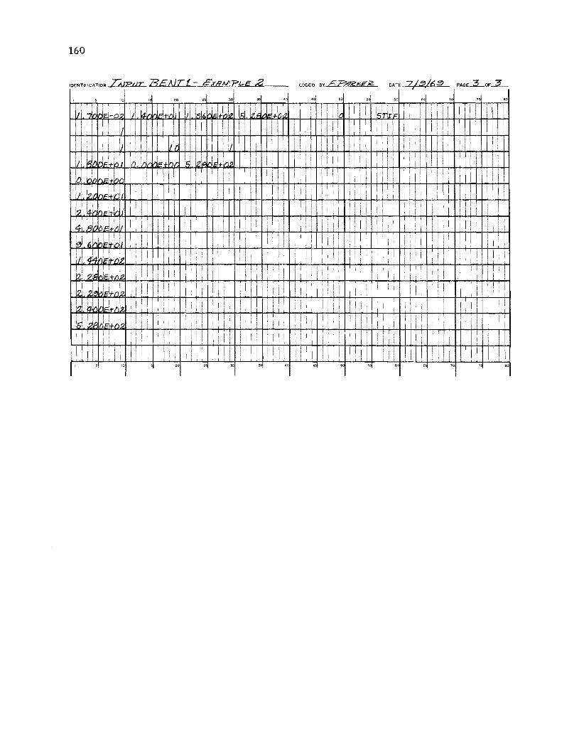
160
IDENTIFICATION TAJP,)T 7? E AiT f - EXRM PI-E 2 , 1 $ 10; I 20; ttl 30 3& '" 4!l 50 5 60 6S 10 1 '0
I ! I
APPENDIX F
OUTPUT FOR EXAMPLE PROBLEMS

!!!!!!!!!!!!!!!!!!!"#$%!&'()!*)&+',)%!'-!$-.)-.$/-'++0!1+'-2!&'()!$-!.#)!/*$($-'+3!
44!5"6!7$1*'*0!8$($.$9'.$/-!")':!

163
EXAMPLE 1 COPANO BAY CAUSEwAy,ARANSAS COUNTY TEXAS,US HIGHwAY 35
LIST OF INPUT DATA
PV PH TM TOL KNPL KOSC 8.4400E+05 3.6400E+04 1.6817E+07 1.0000E .. 03 4 0
CONTROL DATA FOR PILES AT E.ACH LOCATION
PILE NO DISTA DISTB BATTER POTT KS KA 1 -1.2600E+02 o. -2.4400E-Ol 1.0000E+00 1 1 2 -9.0000E+Ol O. O. 2.0000£+00 1 1 3 9.0000E+Ol O. O. 2.0000E+00 1 1 4 1.2600E+02 O. 2.4400E-Ol 1.0000E+OO 1 1
PILE NO. NN HH OPS NOEl CONNECTION FDBET 1 31 3.60000E+Ol 1.20000E+02 1 FIX -0. 2 31 3.60000E+Ol 1.20000E+02 1 FIX -0. 3 31 3.60000E+Ol 1.20000E+02 1 FIX -0. 4 31 3.60000E+Ol 1.20000E+02 1 FIX -0.
RRI XXI XX2 PILE NO 1
4.37400E+I0 o. 1.11600E+03 PILE NO 2
4.37400E+I0 O. 1.11600E+03 PILE NO 3
4.37400E+I0 o. 1.11600E+03 PILE NO 4
4.37400E+I0 O. 1.11600E+03

164
AXIAL LOAD SETTLEMENT DATA
IDENTIFIER 1 ZZZ -1.00000E+Ol -6.50000E-Ol -1.90000E-Ol -1.60000E-Ol -1.40000E"Ol
O. 3.00000E-02 4.00000E-02 5.00000E-02 6.00000E-02 1.40000E-Ol 1.60000E-Ol 1.90000E-Ol 6.50000E"Ol 1.00000E+Ol
INPUT OF SOIL PARAMETERS
SOIL PROFILE NO. 1 STRATUM NO.
GAMMA COHESION TOP DEPTH O. 1.0000E-03 O.
SOIL PROFILE NO. 1 STRATUM NO.
GAMMA COHESION TOP DEPTH 1.7400E .. 02 3.8000E+00 6.0000E·01
SOIL PROFILE NO. 1 STRATUM NO.
GAMMA COHESION TOP DEPTH 1.7400E-02 1.5000E+01 8.9400E+02
SSS -3.60000E+05 -3.60000E+05 .. 2.80000E+05 .. 2.60000E+05 -2.40000E+05
O. 4.00000E+04 8.00000E+04 1.00000E+05 1.20000E·05 2.40000E·05 2.60000E+05 2.80000E+05 3.60000E+05 3.60000E+05
1 TYPE
BOTTEMDEPTH 6.0000E+01
2 TYPE
BOTTEMDEPTH 8.9400E+02
3 TYPE
BOTTEMDEPTH 1.0000E+03
DIAMETER DISTRIBUTION FOR PILE
DIAMETER 1.8000E+Ol
TOP DIS o
BOT DIS 1.0000E+03
SOIL CLAY
CONSISTENCY SOFT
SOIL CLAY
CONSISTENCY SOFT
SOIL CLAY
CONSISTENCY SOFT

165
p.y CURVES SET IDENTIFIER NO. 1 NUMBER OF CURVES IN SET 9
CURVE NO. 1 DEPTH TO CURVE 0
SOIL REACTION DEFLECTION O. O. 3.6000E-02 4.3200E-02 3.6000E-02 1.8000E+02
CURVE NO. 2 DEPTH TO CURVE 6.0000E+Ol
SOIL REACTION DEFLECTION O. O. 6.2613E-02 1.4400E-Ol 8.8548E-02 2.8800E-Ol 1.0845E-Ol 4.3200E-01 1.2523E-Ol 5.7600E-Ol 1.4001E-Ol 7.2000E-Ol 1.5337E-Ol 8.6400E"01 1.6566E-Ol 1.0080E+00 1.7710E-Ol 1.1520E+00 1.8784E-Ol 1.2960E+00 1.9800E-Ol 1.4400E+00 1.9800E-Ol 1.8000E+02
CURVE NO. 3 DEPTH TO CURVE 6.1000E+Ol
SOIL REACTION DEFLECTION O. O. 2.3793E+02 1.4400E-01 3.3648E+02 2.8800E-Ol 4.1211E+02 4.3200E .. Ol 4.7586E+02 5.7600E-Ol 5.3203E+02 7.2000E-Ol 5.8281E+02 8.6400E-Ol 6,2950E+02 1.0080E+00 6.7297E+02 1.1520E+00 7.1379E+02 1.2960E+00 7.5240E+02 1,4400E+00 7.5240E+02 1.8000E+02
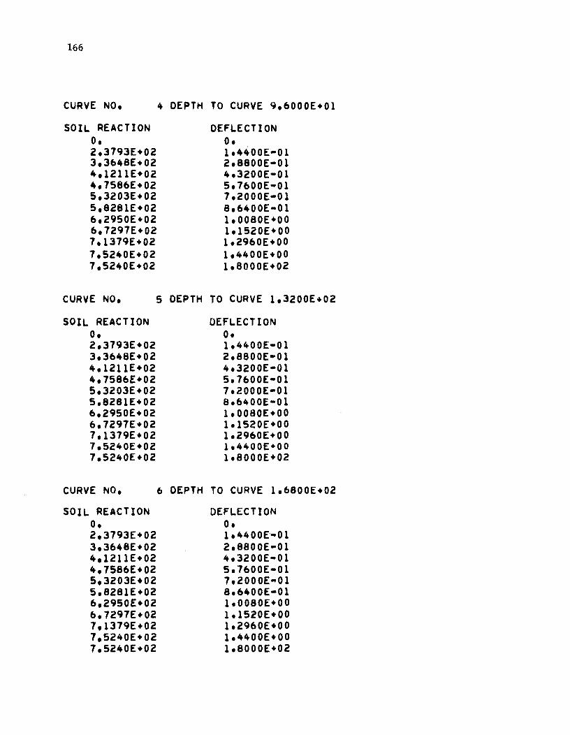
166
CURVE NO. 4 DEPTH TO CURVE 9.6000E+Ol
SOIL REACTION DEFLECTION O. O. 2.3193E+02 1.4400E-Ol 3.3648E+02 2.8800E-01 4.1211E+02 4.3200E-Ol 4.1586E+02 5.1600E-Ol 5.3203E+02 1.2000E-01 5.8281E+02 8.6400E-01 6.2950E+02 1.0080E+00 6.1291E+02 1.1520E+00 1.1319E+02 1.2960E+00 1.5240E+02 1.4400E+00 1.5240E+02 1.8000E+02
CURVE NO. 5 DEPTH TO CURVE 1.3200E+02
SOIL REACTION DEFLECTION O. O. 2.3193E+02 1.4400E-Ol 3.3648E+02 2.8800E-Ol 4.1211E+02 4.3200E-Ol 4.1586E+02 5.1600E-01 5.3203E+02 1.2000E-Ol 5.8281E+02 8.6400E-01 6.2950E+02 1.0080E+00 6.1291E+02 1.1520E+00 1.1319E+02 1.2960E+00 1.5240E+02 1.4400E+00 1.5240E+02 1.8000E+02
CURVE NO. 6 DEPTH TO CURVE 1.6800E+02
SOIL REACTION DEFLECTION O. O. 2,3193E+02 1.4400E .. Ol 3.3648E+02 2.8800E .. Ol 4.1211E+02 4.3200E-Ol 4.1586E+02 5.1600E-01 5.3203E.02 1,2000E"01 5.8281E+02 8.6400E-01 6.2950E+02 1.0080[+00 6.1291E+02 1.1520E+00 1,1319E+02 1.2960E+00 1.5240E+02 1.4400E+00 1.5240E+02 1.8000E+02

167
CURVE NO. 7 DEPTH TO CURVE 2.0400E+02
SOIL REACTION DEFLECTION O. O. 2.3793E+02 1.4400E-01 3.3648E+02 2.8800E ... 01 4.1211E+02 4.3200E-01 4.7586E+02 5.7600E-01 5.3203E+02 7.2000E-01 S.8281E+02 8.6400E ... 01 6.29S0E+02 1.0080E+00 6.7297E+02 1.1520E+00 7.1379E+02 1.2960E+00 7.5240E.02 1.4400E+00 7.S240E.02 1.8000E+02
CURVE NO. 8 DEPTH TO CURVE 2.4000E+02
SOIL REACTION DEFLECTION O. O. 2.3793E.02 1.4400E-01 3.3648E+02 2.8800E-01 4.1211E+02 4.3200E .. 01 4.7S86E+02 5.7600E-01 5.3203E+02 7.2000E-01 5.8281E+02 8.6400E-01 6.2950E+02 1.OO80E+00 6.7297E+02 1.1520E+00 7.1379E+02 1.2960E+00 7.5240E+02 1.4400E+00 7.5240E+02 1.8000E+02
CURVE NO. 9 DEPTH TO CURVE 9.9600E+02
SOIL REACTION DEFLECTION O. O. 9.3920E+02 1.4400E-01 1.3282E+03 2.tl800E-01 1.6267E+03 4.3200E-01 1.8784E+03 5.7600E-01 2.1001E+03 7.2000E-Ol 2.3006E+03 8.6400E ... Ol 2.4849E+03 1.0080E·00 2.6564E·03 1.1520E+00 2.8176E·03 1.2960E+OO 2.9700E+03 1.4400E+OO 2.9700E+03 1.8000E+02

168
EXAMPLE 1 COPANO BAY CAUSEWAY. ARANSAS COUNTY TEXAS. US HIGHWAY 35
PILE NUM 1
DISTA.IN -1.26000E+02
PX.LB XT.IN 7.87213E+04 3.96803E-02 INPUT INFORMATION
DISTB.IN o.
THETA.RAD -2.44000E-01
PT.LB MT.IN-LB YT.IN 1.73414E+03 -2.53284E+05 1.13355E-01
TC TOP DIA.IN INC. LENGTH.IN NO. OF INC KS KA
FIX 1.8000E+01 3.6000E+01 31 1 1
PILE LENGTH.IN DEPTH TO SOIL ITERATION TOL.BOUNDRY CONU.2
1.1160E+03 1.2000E+02 1.0000E-03 -8.5355E.-05
XtIN
O. 3.60000E+01 7.20000E+01 1.08000E+02 1.44000E+02 1.80000E+02 2.16000E+02 2.52000E+02 2.88000E+02 3.24000E+02 3.60000E+02 3.96000E+02 4.32000E+02 4.68000E+02 5.04000E+02 5.40000E+02 5.7bOOOE+02 6.12000E+02 6.48000E+02 6.84000E+02 7.20000E+02 7.56000E+02 7.92000E+02 8.28000E+02 8.64000E+02 9.00000E+02 9.36000E+02 9.72000E+02 1.00800£+03 1.04400E+03 1.08000E+03 1.11600E+03
Y. IN
1.13356E-01 1.06531E-01 9.40663E-02 7.78418E-02 5.97446E-02 4.16668E-02 2.54989E-02 1.31266E-02 4.80862E-03
-3.84352E-05 -2.31125E-03 -2.91006E-03 -2.59236E-03 -1.90724E-03 -1.19396E-03 -6.19929E-04 -2.33925E-04 -1.73543E-05
7.61099E-05 9.52659E-05 7.88339E-05 5.19377E-05 2.77032E-05 1.08677E-05 1.43275E-06
-2.56472E-06 -3.37009E-06 -2.73087E-06 -1.70396E-06 -7.60450E-07
9.98285E-09 6.94984E-07
OUTPUT INFORMATION
MOMENT.IN-LB
-2.53286E+05 -1.90319E+05 -1.26909E+05 -6.32023E+04
6.51531E+02 6.44624E+04 1.28099E+05 1.36835E+05 1.17143E+05 8.68804E+04 5.64976E+04 3.09322E+04 1.24008E+04 9.49911E+02
-4.69949E+03 -6.34589E+03 -5 .71840E + 03 -4.15483E+03 -2.50790E+03 -1.20110E+03 -3.53170E+02
8.98372E+01 2.49713E+02 2.49771E+02 1.83514E+02 1.07733E+02 4.87547E+01 1.30849E+01
-2.81491E+00 -5.84134E+00 -2.88334E+00 -4.65745E+01
ES.LB/IN
O. O. O. O. 5.35396E-01 4.34813E-01 1.65229E+03 1.65229E+03 1.65229E+03 1.65229E+03 1.65229E+03 1.88419E+03 2.11609E+03 2.34799E+03 2.57989E+03 2.81179E+03 3.043b9E+03 3.21559E+03 3.50749E+03 3.73939E+03 3.97129E+03 4.20319E+03 4.43509E+03 4.66699E+03 4.89890E+03 5.13080E+03 5.36210E+03 5.59460E+03 5.82650E+03 6.05840E+03 6.29030E+03 6.52220E+03
P LB/IN
-0. -0. -0. -0. -3.19871E-02 -1.81173E-02 -4.21316E+01 -2.16889E+01 -7.94523E+00
6.35061E-02 3.81886E+00 5.48311E+00 5.48568E+00 4.47817E+00 3.08029E+00 1.74311E+00 7.11995E-01 5.68458E-02
-2.66955E-01 -3.56231E-01 -3.13073E-01 -2.18304E-01 -1.22866E-01 -5.07194E-02 -7.01889E-03
1.31590E-02 1.80"728E-02 1.52781E-02 9.92812E-03 4.60711E-03
-6.27951E-05 "'4.53282E-03

169
EXAMPLE 1 COPANO BAY CAUSEWAy.ARANSAS COUNTY TEXAS.US HIGHWAY 35
PILE NUM 2
OISTA.IN ~9.00000E+Ol
PX.L8 XTtlN 1.33444E+05 b.89621E~02
INPUT INFORMATION
DISTB.IN o.
THETA.RAO O.
PT.LB MT.IN-LB YT.IN 1.49018E+03 -2.18916E+05 1.00411E-Ol
TC TOP DIA.IN INC. LENGTH.IN NO. OF INC KS KA
FIX 1.8000E+Ol 3.6000E+Ol 31 1 1
PILE LENGTH.IN DEPTH TO SOIL ITERATION TOL.80UNORY COND.2
1.llbOE+03 1.2000£+02 1.0000E-03 -8.~355E-05
XtlN
O. 3.60000E+Ol 1.20000E+Ol 1.08000E+02 1.44000E+02 1.80000E+02 2.16000E+02 2.52000E+02 2.88000E+02 3.24000E+02 3.60000E+02 3.96000E+02 4.32000E+02 4.68000E+02 5.04000E+02 5.40000E+02 5.16000E+02 6.12000E+02 6.48000E·02 6.84000E+02 1.20000E+02 1.56000E+02 1.92000E+02 8.28000E+02 8.64000E+02 9.00000E+02 9.36000E+02 9.12000E+02 1.00800E+03 1.04400E+03 1.08000E+03 1.11600E+03
YtlN
1.00405E-Ol 9.40888E-02 8.29018E-02 6.t:i4181E-02 5.24649E-02 3.65151E-02 2.22826E-02 1.14101E-02 4.11592E-03
-1.20516E-04 -2.09294E-03 -2.59642E-03 -2.29901E-03 -1.68411E-03 -1.04952E-03 -5.41300E-04 -2.01038E-04 -1.12041E-05
6.98209E-05 8.54915E-05 1.01384E-05 4.59029E-05 2.42895E-05 9.31130E-06 1.08239E-06
-2.38590E-06 -3.04095E~06
-2.43116E-06 -1.50110E-06 -6.63465E-01
2.23410E-08 6.31418E-01
OUTPUT INFORMATION
MOt-lENT.IN-LB
-2.18910E+05 -1.64399E+05 -1.09238E+05 -5.36455E+04
2.15953E+03 5.19162E+04 1.13423E+05 1.20161E+05 1.03199E+05 1.b4103E+04 4.95111E+04 2.10291E+04 1.01151E+04 6.64258E+02
-4.26510E+03 -5.66849E+03 -5.01693E+03 -3.61221E+03 -2.20553E+03 "1.04145E+03 -2.99518E+02
8.84938E+Ol 2.26161E+02 2.23333E+02 1.62898E+02 9.49412E+Ol 4.24858E+Ol 1.09911E+Ol
-2.81609£+00 -5.34101E+00 -2.58158E+00 -4.18108E+Ol
ES.LB/IN
O. O. O. O. 5.85543E-Ol 4.34813E-Ol l.b5229E+03 1.65229E+03 1.65229E+03 1.65229E+03 1.65229E+03 1.88419E+03 2.11609E+03 2.34199E+03 2.51989E+03 2.81119E+03 3.04369E+03 3.21559E+03 3.50149E+03 3.13939E+03 3.91129E+03 4.20319E+03 4.43509E+03 4.66699E+03 4.89890E+03 5.13080E+03 5.36210E+03 5.59460E+03 5.82650E+03 6.05840E+03 6.29030E+03 b.52220E+03
P U4/IN
-0. -0" -0. -0. -3.01205E-02 -1.58115E-02 -3.b8113E+Ol -1.88~28E+Ol -6.80069E+00
1.99121E-Ol 3,,45815E+00 4.89215(+00 4.86492E+00 3.95421E+00 2.10164E+00 1.52202E+00 6.11899E-01 3,,61022E-02
-2.44896E'-01 -3.19109E-01 -2.18540E-01 -1.92939E-01 -1.01126E-01 -4.31638E-02 -5.30252E-03
1.22416E-02 1.63011E.-02 1.36349E-02 8.18463E-03 4.01954E-03 -1.40~32E-04 -4,,111363£-03

170
EXAMPLE 1 COPANO BAY CAUSEWAY. ARANSAS COUNTY TEXAS,US HIGHWAY 35
PILE NUM 3
DISTA,IN 9.00000E+Ol
PX.LB XT.IN 1.56490E+05 8.43266E-02 INPUT INFORMATION
DISTB,IN O.
PT.LB 1.48246E+03
THETA,RAO O.
MT.IN-LB YT.IN -2.18831E+05 1.00411E-Ol
TC TOP DIA.IN INC. LENGTH.IN NO. OF INC KS KA
FIX 1.8000E+Ol 3.6000E+Ol 31 1 1
PILE LENGTH.IN DEPTH TO SOIL ITERATION TOL.BOUNDRY COND.2
1.1160E+03 1.2000E+02 1.0000E-03 -8.5355E-05
X. IN
O. 3.60000E+Ol 1.20000E+Ol 1.08000E+02 1.44000E+02 1.80000E+02 2.16000E+02 2.52000E+02 2.88000E+02 3.24000E+02 3.60000E+02 3.96000E+02 4.32000E+02 4.68000E+02 5.04000E+02 5.40000E.02 5.16000E+02 6.12000E+02 6,48000E.02 6.84000E+02 1.20000E+02 1.56000E+02 1.92000E+02 8.l8000E+02 8.64000E+02 9.00000E+02 9.36000E.02 9,12000E+02 l,00800E+03 1.04400E+03 1.08000E+03 1.11600E+03
YeIN
1.00399E-Ol 9.40848E-02 8.28911E-02 6.84695E-02 5.24501E-02 3.64945E-02 2.22568E-02 1.13826E ... 02 4.08953E-03
-1.43336E-04 -2.11012E-03 -2.60812E~03 -2.30634E"03 -1.68153E-03 -1.05032E-03 -5.40631E-04 -1.99802E-04 -9.95169E-06
1.01998E-05 8.61335E-05 1.04139E-05 4.60210E-05 2.42925E-05 9.32845E-06 1.02450E"'06
-2.43243E-06 -3.01062E ... 06 -2,45211E-06 -1.51269E-06 -6.62445E-01
2.11212E-08 6,39461E-01
OUTPUT INFORMATION
MOMENT.IN-LB
-2.18824E+05 -1.64461E+05 "1.09348E+05 -5.31215E+04
2.15391E+03 5.79195E+04 1.13516E+05 1.20866E+05 1.03281E+05 1.64600E+04 4.95915E+04 2.10130E+04 1.06194E+04 6.21345E+02
-4.30443E+03 ... 5.69841E+03 ... 5.09596E+03 -3.68168E+03 -2.20805E+03 -1.04602E+03 -2.96511E+02
9.15413E+Ol 2.28505E+02 2.24118E·02 1.63581E+02 9.51325E+Ol 4.24116E+01 1.08351E+Ol
-3.01202E+00 -5.42263E+00 ... 2.60618E+00 -4.22481E+Ol
ES.LB/IN
O. O. O. O. 5.85659E-Ol 4.34813E-Ol 1.65229E+03 1.65229E+03 1.65229E+03 1.65229E+03 1.65229E+03 1.88419E+03 2.11609E+03 2.34199E+03 2.51989E+03 2.81119E+03 3.04369E+03 3.21559E+03 3.50149E+03 3.13939E+03 3.91129E+03 4.20319E+03 4.43509E+03 4.66699E+03 4.89890E+03 5.13080E+03 5.36210E+03 5.59460E+03 5.82650E+03 6.05840E+03 6.29030E+03 6.52220E+03
P L8/IN
-0. -0. -0. -0. -3.07119E-02 -1.58683E-02 -3.61141E+Ol -1.88013E+Ol -6.15109E+00
2.36833E-Ol 3.48152E+00 4.91533E+00 4.88043E+00 3.96231E+00 2.10910E+00 1.52016E+00 6.08135E-Ol 3.26113E-02
-2.48330E-Ol -3.22081E-01 -2.19813E-Ol -1.93461E-01 -1.01139E-Ol -4.35358E-02 -5.01893E-03
1.24803E-02 1.64668E-02 1.31189E-02 8.81366E-03 4.01335E-03
-1.10638E-04 -4.11069E-03

171
EXAMPLE 1 COPANO SAY CAUSEWAY,ARANSAS COUNTY TEXAS,US HIGH~AY 35
PIL.E NUM 4
DISTA,IN 1.26000E+02
PX,L.8 Xl,IN 1.93603E+05 1.09068E.01 INPUT INFORMATION
DISTB,IN O.
PT,L.B 1.06245E+03
THETA,RAD 2.44000E-Ol
MT,IN-LB YT,IN -1.55201E+05 7.63223£-02
TC TOP DIA,IN INC. LENGTH,IN NO. OF INC KS KA
FIX 1.8000E+01 3.6000E+01 31 1 1
PILE LENGTH,IN DEPTH TO SOIL ITERATION TOL.80UNDRY COND.2
1.1160£+03 1.2000E+02 1.0000E ... 03 -8.5355£-05
XtlN
O. 3.60000E+Ol 7.20000E+Ol 1.08000E+02 1.44000E+02 1.80000E+02 2.16000E+02 2.52000E+02 2.88000E+02 3.24000E+02 3.60000E+02 3.96000E+02 4.32000E+02 4.68000E+02 5.04000E+02 5.40000E+02 5.76000E+02 6.12000E+02 6.48000£+02 6.84000E+02 7.20000E+02 7.56000E+02 7.92000E+02 8.28000E+02 8.64000E+02 9.00000E+02 9.36000E+02 9.72000E+02 1.00800E.03 1.04400E+03 1.08000E+03 1.11600E+03
Y,IN
7.62891E-02 7.09170E"02 6.21102E-02 5.10527E-02 3.89411E .. 02 2.69781E-02 1.63647E-02 8.29365E-03 2.90464E-03
-2.04055E-04 -1.63161E-03 -1.97387E-03 -1.72940E-03 -1.25731E-03 -7.77498E-04 -3.96529E"04 -1.43383E-04 .. 3.49209E-06
5.51189E-05 6.53318E-05 5.28818E-05 3.42531E·05 1.79008E-05 6.73851E-06 6.01402E-07
-1.91182E-06 -2.33636E-06 -1.84273E-06 -1.12561E-06 -4.85053E-07
3.11518E-08 4.88774E-07
OUTPUT INFORMATION
MOMENT,IN-LB
-1.55206E+05 -1.15918E+05 -7.59645E+04 -3.55755E+04
5.01770E+03 4.55481E+04 8.58019E+04 9.05207E+04 7.69604E+04 5.67387E+04 3.66285E+04 1.98021E+04 7.68209E+03 2.60804E+02
-3.33599E+03 -4.31404E+03 -3.82237£+03 -2.74318E+03 -1.63344E+03 -7.64871E+02 -2.08533E+02
7.68293E+Ol 1.75163E+02 1.69600E+02 1.22306E·02 7.04930E+Ol 3.09880E+Ol 7.54313E·00
-2.58413E+00 -4.19692E+00 -1.97715E+00 -3.19409E+Ol
ES,LB/IN
O. O. O. O. 6.73925£-01 4.34813E-Ol 1.65229E+03 1.65229E+03 1.65229E+03 1.65229E+03 1.65229£+03 1.88419E+03 2.11609E+03 2.34799E+03 2.51989E+03 2.81179E+03 3.04369E+03 3.27559E+03 3.50749E+03 3.73939E+03 3.97129E+03 4.20319E+03 4.43509E+03 4.66699E+03 4.89890E+03 5.13080E+03 5.36270E+03 5.59460E+03 5.82650E+03 6.05840£+03 6.29030E+03 6.52220E+03
P LI;/IN
-0. -0. -0. -0. ~2.62434E-02
-1.17304E-02 ~2.70393E+01 "1.37035E+Ol "'4.79931E+00
3.37158E-Ol 2.69589E+00 3.71914E+00 3.65956£+00 2.95216E+00 2.00586E+00 1.11496E+00 4.36413E-01 1.14386E-02
-1.93329E-01 -2.44301E-01 -2.10009E-01 -1.43972E-Ol -7.93917E-02 -3.14486E-02 -2.94621E-03
9.80915E-03 1.25292£~02
1.03094E .. 02 6.55836E-03 2.93864E-03
-1.95954E-04 -3.18788E-03

112
EXAMPLE 2 HOUSTON SHIP CHANNEL BRIDGE,HARRIS CO.,HIGHWAY 1-610
LIST Of' INPUT DATA .... -PV PH TM TOL KNPL KOSC
2.7600[+07 1.1260E+06 8.6568E+08 1.0000E-03 6 0
CONTROL DATA FOR PILES AT EACH LOCATION
PILE NO DISTA OISTB BATTER POTT KS KA 1 -1.S000E+02 O. -1.6600E-Ol 2.4000[+01 1 1 2 -9.0000E+01 O. -8.3000E-02 2.3000E+Ol 1 1 3 -3.0000E+01 O. -4.2000E-02 2.4000E+Ol 1 1 4 3.0000E+01 O. 4.2000E-02 2.4000E+Ol 1 1 5 9.0000E+01 O. 8.3000E-02 2.3000E+01 I 1 6 1.5000[+02 O. 1.6600E-Ol 2.4000E+01 1 1
PILE NO. NN HH OPS NOEl CONNECTION FDBET 1 33 1.60000E+01 O. 1 FIX -0. 2 33 1.60000E+01 O. 1 FIX -0. 3 33 1.60000E+01 O. 1 FIX -0. 4 33 1.60000E+01 O. 1 FIX -0. 5 33 1.60000E+01 O. 1 FIX -0. 6 33 1.60000E+01 O. 1 FIX -0.
RRI XXI XX2 PILE NO 1
4.37400E+10 O. 5.28000E+02 PILE NO 2
4.37400E+10 O. 5.28000E+02 PILE NO 3
4.37400E+10 O. 5.28000E+02 PILE NO 4
4.37400E+10 O. 5.28000E+02 PILE NO 5
I+.37400E+10 O. S.28000E+02 PILE NO 6
4.37400E+10 O. 5.28000E+02

AXIAL LOAD SETTLEMENT DATA
IDENTIFIER 1 ZZZ -1.00000E+Ol -5.00000E-01 o. 5.00000E-01 1.00000E+01
INPUT OF SOIL PARAMETERS
SSS -6.00000E+05 -6.00000E+05
O. 6.50000E.05 6.50000E·05
173
SOIL PROFILE NO. 1 STRATUM NO. 1 TYPE SOIL SAND
GAMMA ANGLE OF FRIC. TOP DEPTH BOTTEM DEPTH DENSITY 3.0000E-02 6.0000E-01 O. 1.5600E+02 DENSE
SOIL PROFILE NO. 1 STRATUM NO. 2 TYPE
GAMMA COHESION TOP DEPTH BOTTEMDEPTH 1.7000E ... 02 1.4000E+01 1.5600E+02 5.2800E·02
DIAMETER DISTRIBUTION FOR PILE
DIAMETER 1.8000E·01
TOP DIS o
BOT DIS 5.2800E·02
SOIL CLAY
CONSISTENCY STH-

174
p-y CURVES SET IDENTIFIER NO. 1 NUMBER OF CURVES IN SET 10
CURVE NO. 1 DEPTH TO CURVE 0
SOIL REACTION DEFLECTION O. O. O. 1.0000E+00 O. 1.8000E+02
CURVE NO. 2 DEPTH TO CURVE 1.2000E+Ol
SOIL REACTION DEFL.ECTION O. O. 3.3634E+01 8.4085E-02 3.3634E+Ol 1.8000E+02
CURVE NO. 3 DEPTH TO CURVE 2.4000E+Ol
SOIL REACTION DEFLECTION O. O. 9.1565E+Ol 1.1446E ... Ol 9.1565E+Ol 1.8000E+02
CURVE NO. 4 DEPTH TO CURVE 4.8000E+Ol
SOIL REACTION DEFLECTION O. O. 2.8032E+02 1.7520E"'01 2.8032E+02 1.8000E+02
CURVE NO. 5 DEPTH TO CURVE 9.6000E+Ol
SOIL. REACTION DEFLECTION O. O. 9.4939E+02 2. 9668E ... Ol 9.4939E+02 1.8000E+02
CURVE NO. 6 DEPTH TO CURVE 1.4400E+02
SOIL REACTION DEFLECTION O. O. 2.0072E+03 4.1817E-Ol 2.0072E+03 1.8000E+02

CURVE NO.
SOIL. REACTION O. 8.7658E+02 1.2397E+03 1.5183E+03 1.7532E+03 1.9601E+03 2.1472E.03 2.3192E·03 2.4794E·03 2.6298E·03 2.7720E·03 2.7720E+03
CURVE NO.
SOIL. REACTION O. 8.7658E+02 1.2397E·03 1.5183E+03 1.7532£·03 1.9601E.03 2.1472E+03 2.3192E+03 2.4794E+03 2.6298E+03 2.7720E+03 2.7720E.03
CURVE NO.
SOIL. REACTION O. 8.7658E+02 1.2397E·03 1.5183E.03 1.7532E+03 1.9601E+03 2.1472E+03 2.3192E+03 2,4794E+03 2,6298E+03 2,7720E+03 2,7720E+03
7 DEPTH TO CURVE 2.2800E+02
DEFL.ECTION
8 DEPTH
9 DEPTH
O. 3.6000E-02 7.2000E-02 1.0800E-01 1.4400E-Ol 1.8000E-Ol 2.1600E-Ol 2.5200E-Ol 2.8800E-Ol 3.2400E-Ol 3.6000E-Ol 1.8000E+02
TO CURVE 2.2900E+02
DEFL.ECTION O. 3.6000E-02 7.2000E-02 1.0800E-Ol 1.4400E-Ol 1.8000E-01 2.1600£-01 2.5200E-Ol 2.8800E-01 3.2400£-01 3.6000E"'01 1.8000E·02
TO CURVE 2.4000E+02
DEFL.ECTION O. 3.6000E-02 7.2000£-02 1.0800£-01 1.4400E-01 1.8000E-Ol 2.1600E-Ol 2.5200E-01 2.8800E-01 3,2400E-Ol 3.6000E-01 1,8000E+02
175

176
CURVE NO. 10 DEPTH TO CURVE 5.2800E+02
SOIL REACTION DEflECTION O. 8.1658E+02 1.2397E+03 1.5183£·03 1.1532E+03 1.9601E+03 2.1472E+03 2.3192E+03 2.4794£+03 2.6298£+03 2.7720E+03 2.7720.E+03
O. 3.6000E·02 7.2000E-02 1.0800E-01 1.4400E-01 1.8000E .. 01 2.1600E-01 2.5200E .. 01 2.8800E-01 3.2400E-01 3.6000E-01 1.8000E+02

177
EXAMPLE 2 HOUSTON SHIP CHANNEL BRIDGE,HARRIS CO.,HIGH~AY 1-610
PILE NUM 1
DISTA,IN .. 1.S0000E+02
PX,L8 XT,IN 1.0631SE+OS 8.11810E-02 INPUT INFORMATION
OISTB,IN O.
PT,LB 3.28131E+03
THETA,RAO -1.66000E-Ol
MT,IN-LB YT,IN -4.59889E+04 4.13128E-02
TC TOP DIA,IN INC. LENGTH.IN NO. OF INC KS t<A
FIX 1.8000E+01 1.6000E+01 33 1 1
PILE LENGTH,IN DEPTH TO SOIL ITERATION TOL.BOUNDRY COND.2
S.2800E+02 O.
XtIN
O. 1.60000E+01 3.20000E+01 4.80000E+01 6.40000E+01 8.00000E+Ol 9.60000E+01 1.12000E+02 1.28000E+02 1.44000E+02 1.60000E+02 1.16000E+02 1.92000E+02 2.08000E+02 2.24000E+02 2.40000E+02 2.S6000E+02 2.12000E+02 2.88000E+02 3.04000E+02 3.20000E+02 3.36000E+02 3.S2000E+02 3.68000E+02 3.84000E+02 4.00000E+02 4.16000E+02 4.32000E+02 4.48000E+02 4.64000E+02 4.80000E+02 4.96000E+02 S.12000E+02 S.28000E+02
Y,IN
4.68923E-02 4.00S64E-02 3.3246SE-02 2.61428E-02 2.01120E-02 1.S496SE-02 1.10116E-02 1.3504SE-03 4.49281E-03 2.31682E-03 9.1141SE-04
-1.19363E-OS -S.131S1E-04 ... 1.14610E-04 -1.229S4E-04 -6.26216E-04 .. 4.86164E-04 -3.43184E-04 -2.1894SE-04 -1.21302E-04 -S.190S4E-OS -1.36313E-06
1.16264E-OS 2.864S4E-OS 3.06421E ... OS 2.1S248E-OS 2.20813E-OS 1.61201E-OS 1.0610SE-OS S.95380E-06 2.16006E-06
-9.18919E-01 -3.15019E-06 -6.40131E-06
1.0000E-03 -4.1831E-04
OUTPUT INFORMATION
MOMENT.IN-LB
-4.88633E+04 4.46043E+03 S.23123E+04 9.10S32E+04 1.18184E+OS 1.3S096E+OS 1.4014SE+OS 1.31286E+OS 1.26116E+OS 1.11160E+OS 9.2614SE+04 1.20225E+04 S.14231E+04 3.28922E+04 1.19438E+04 1.318SSE+03 S.92S90E+02
-3.099S1E+03 -4.64610E+03 -4.82621E+03 -4.246S9E+03 -3.34011E+03 -2.38691E+03 -1.S41S1E+03 -8.13164E+02 -3.96423E+02 -9.04101E+01
1.19116E+Ol 1.4S828E+02 1.41448E+02 1.11863E+02 6.21436E+01 1.96811E+Ol 1.S4866E+03
ES,LB/IN
1.81899E-12 S.33333E+02 1.06661E+03 1.60000E+03 2.13333E+03 2.66661E+03 3.20000E+03 3.13333E+03 4.26661E+03 4.80000E+03 8.52312E+03 1.22414E+04 1.S9112E+04 1.96949E+04 2.34186E+04 2.4349SE+04 2.4349SE+04 2.4349SE+04 2.4349SE+04 2.4349SE+04 2.4349SE+04 2.4349SE+04 2.4349SE+04 2.43495E+04 2.4349SE+04 2.4349SE+04 2.4349SE+04 2.4349SE+04 2.4349SE+04 2.4349SE+04 2.4349SE+04 2.4349SE+04 2.4349SE+04 2.4349SE+04
P LB/IN
-8.S2961E-14 -2.13634E+Ol -3.S4629E+Ol -4.21885E.+Ol ... 4.43131E+Ol -4.13239E+01 -3.S2311E+01 -2.14411E+Ol -1.91693E+01 -1.14081E+Ol -1.1b865E+00
1.46189E·01 8.20S30E+00 1.40142E+01 1.69306E+Ol 1.52495E+Ol 1.18525E+Ol 8.31099E+00 S.33121E+00 2.95364E+00 1.26381E+00 1.19289E·Ol
-4.29194E-01 -6.91S03E-Ol -1.46121E-Ol -6.10216E-Ol -S.31811E-Ol -3.92S33E-Ol -2.S8361E-01 -1.44912E-Ol -5.2S964E-02
2.38311E-02 9.13300E-02 1.56011E-01

178
EXAMPLE 2 HOUSTON SHIP CHANNEL BRIDGE,HARRIS co. ,HIGHWAY 1-610
PILE NUM 2
DISTA,IN -9.00000E+Ol
PX,LB XT,IN 1.43511E+05 1.10439E-Ol INPUT INfORMATION
DISTB,IN O.
PT,LB 2.52241E+03
THETA,RAD -8.30000E-02
MT,IN-LB YT,IN 3.91335E+02 4.25105E-02
TC TOP DIA,IN INC. LENGTH,IN NO. OF INC KS KA
FIX 1.8000E+Ol 1.6000E+Ol 33 1 1
PILE LENGTH,IN DEPTH TO SOIL ITERATION TOL.BOUNDRY COND.2
5.2800E+02 O.
X,IN
O. 1.60000E+Ol 3.20000E+Ol 4.80000E+Ol 6.40000E+Ol 8.00000E+Ol 9.60000E+Ol 1.12000E+02 1.28000E+02 1.44000E+02 1.60000E+02 1.16000E+02 1.92000E+02 2.08000E+02 2.24000E+02 2.40000E+02 2.56000E+02 2.12000E+02 2.88000E+02 3.04000E+02 3.20000E+02 3.36000E+02 3.52000E+02 3.68000E+02 3.84000E+02 4.00000E+02 4.16000E+02 4.32000E+02 4.48000Et02 4.64000E+02 4.80000E+02 4.96000E·02 5.12000E+02 5.28000E+02
Y,IN
4.21030E-02 3.54041E-02 2.89352E-02 2.29096E-02 1.14941E-02 1.21999E-02 8.88188E-03 5.14299E-03 3.34299E .. 03 1.60881E-03 4.45101E-04
-2.53494E-04 -6.01180E-04 -1.01861E-04 -6.66246E-04 -5.50680E-04 -4.11592E-04 -2.19339E-04 -1.69259E-04 -8.64181E"05 -2.99248E-05
4.64930E-06 2.26028E-05 2.91386E-05 2.86449E-05 2.44522E-05 1.88495E-05 1.32348E-05 8.31824E-06 4.32613E .. 06 1.18283E-06
-1.34944E"06 -3.54913E-06 -5.64815E-06
1.0000E-03 -4.1831E-04
OUTPUT INfORMATION
MOMENT,IN-LB
.. 2.02109E+03 3.92933E+04 1.51469E+04 1.04236E+05 1.23253E+05 1.32612E+05 1.33123E+05 1.26245E+05 1.13112E+05 9.15526E+04 1.92140E+04 5.99562E+04 4.13829E+04 2.52352Et04 1.26353E+04 4.01902E+03
-1.16199E+03 -3.18836E+03 .. 4.66430E+03 -4.48124E+03 "3.15536E+03 -2.83919E+03 -1.95081E+03 "1.20108E+03 -6.31986E+02 -2.40914E+02 -2.06183E+00
1.19294E+02 1.58050E+02 1.44822E+02 1.04502E+02 5.61213E+01 1.13043E·Ol 1.32318E+03
ES,LB/IN
1.81899E-12 5.33333E+02 1.06661E+03 1.60000E+03 2.13333E+03 2.66661E+03 3.20000E+03 3.13333E+03 4.26661E+03 4.80000E+03 8.52312E+03 1.22414E+04 1.59112E+04 1.96949E+04 2.34186E+04 2.43495E+04 2.43495E+04 2.43495E+04 2.43495E+04 2.43495E+04 2.43495E+04 2.43495E+04 2.43495E+04 2.43495E+04 2.43495E+04 2.43495E+04 2.43495E+04 2.43495E+04 2.43495E+04 2.43495E+04 2.43495E+04 2.43495E+04 2.43495E+04 2.43495E+04
P LB/IN
-1.65850E-14 ""1.88822E+01 -3.08642E+Ol -3.66554E+01 -3.13201E+01 -3.41331E+01 -2.84220E+01 -2.14405E+Ol -1.42634E+01 -1.12251E+00 -3.19904E+00
3.10465E+00 9.61112E+00 1.39412E+Ol 1.56026E+01 1.34088E+01 1.00221E+01 6.80118E+00 4.12138E+00 2.10510E+00 1.28655E .. 01
-1.13208E-Ol -5.50361E-01 -1.09513E-01 -6.91489E-01 -5.95400E-Ol -4.58911E-01 -3.22261E-01 -2.02545E-Ol -1.05354E-01 -2.88013E"02
3.28583E-02 8.64344E-02 1.31544E-Ol

179
EXAMPLE 2 HOUSTON SHIP CHANNEL BRIDGE,HARRIS CO.,HIGHWAY 1·610
PILE NUM 3
DISTA,IN ",3.00000E.01
PX,LB XT,IN 1.78315E.05 1.37165E-01 INPUT INfORMATION
DISTB,IN O.
PT,LB 1.97946E+03
THETA,RAD ",4.20000E-02
MT,IN"'LB YT,IN 3.28630E+04 3.90018E-02
TC
fIX
TOP DIA,IN INC. LENGTH,IN NO. Of INC KS KA
1.8000E+01 1.6000E+01 33 1 1
PILE LENGTH,IN DEPTH TO SOIL ITERATION TOL.BOUNDRY COND.2
5.2800E+02 O.
XeIN
O. 1.60000E+01 3.20000E+01 4.80000E+01 6.40000E+01 8.00000E+01 9.60000E+01 1.12000E+02 1.28000E+02 1.44000E+02 1.60000E+02 1.76000E+02 1.92000E+02 2.08000E+02 2.24000E+02 2.40000E+02 2.56000E+02 2.72000E+02 2.88000E+02 3.04000E+02 3.20000E+02 3.36000E+02 3.52000E+02 3.68000E+02 3.84000E+02 4.00000E+02 4.16000E+02 4.32000E+02 4.48000E+02 4.64000E+02 4.80000E+02 4,96000E+02 5.12000E+02 5.28000E+02
YeIN
3.87067E-02 3.21048E"'02 2.58772E-02 2.01902E-02 1.51681E-02 1.08861E-02 7.36999E-03 4.60156E-03 2.52628E-03 1.06323E-03 1.14681E-04
-4.25283E-04 -6.64460E-04 -7.03158E-04 .. 6.25999E-04 -4.96972E-04 -3.58157E-04 -2.33513E-04 -1.33916E-04 .. 6. 16985E .. 05 "1.42782E-05
1.32044E-05 2.61503E"05 2.94939E-05 2.72257E-05 2.22659E-05 1.65444E-05 1.11793E-05 6.68507E-06 3.16714E-06 4.86142E-07
-1.61372E-06 -3.40658E-06 ",5.10805E .. 06
1.0000E-03 -4.1831E-04
OUTPUT INfORMATION
MOMENT,IN-LB
3.11152E+04 6.39638E+04 9.23622E+04 1.13598E+05 1.26445E+05 1.30877E+05 1.27740E+05 1.18433E+05 1.04604E+05 8.79068E+04 6.98112E+04 5.13924E+04 3.42535E+04 1.97955E+04 8.86207E+03 1.67239E+03
-2.42117E+03 "4.27964E+03 -4.67804E+03 -4.23680E+03 -3.40655E+03 -2.48373E+03 -1.64063E+03 -9.58832E+02 -4.59878E·02 -1.30155E+02
6.09099E+01 1.48782E+02 1.66813E+02 1.42999E+02 9.92927E+01 5.24527E+01 1.56171E+01 1.16347E+03
ES,LB/IN
1.81899E-12 5.33333E+02 1.06667E+03 1.60000E+03 2.13333E+03 2.66667E+03 3.20000E+03 3.73333E+03 4.26667E+03 4.80000E+03 8.52372E+03 1.22474E+04 1.59712E+04 1.96949E+04 2.34186E+04 2.43495E+04 2.43495E+04 2.43495E+04 2.43495E+04 2.43495E+04 2.43495E+04 2.43495E+04 2.43495E+04 2.43495E+04 2.43495E+04 2.43495E+04 2.43495E+04 2.43495E+04 2.43495E+04 2.43495E+04 2.43495E+04 2.43495E+04 2.43495E+04 2.43495E+04
P LB/IN
-7.04071E-14 -1.71226E+01 -2.76024E+01 -3.23044E+01 -3.23587E+01 -2.90295E+01 -2.35840E+01 -1.71792E+01 -1.07788E+01 -5.10352E+00 -9.77511E-01
5.20863E+00 1.06122E+01 1.38486E+01 1.46600E+Ol 1.21010E+01 8.72096E+00 5.68592E+00 3.26079E+00 1.50233E+00 3.47667E-01
-3.21521E-01 -6.36747E-01 -7.18162E-01 .. 6.62932E-01 .. 5.42164E-01 -4.02848( .. 01 -2.72211E-01 -1.62778E-01 -7.71184E-02 -1.18373E-02
3.92933E-02 8.29487E-02 1.24379E-01

180
EXAMPLE 2 HOUSTON SHIP CHANNEL BRIDGE,HARRIS CO.,HIGHwAY I-b10
PILE NLIM 4
DISTA,IN 3.00000E+01
PX,L8 XT,IN 2.14540E+05 1.65031E~01
INPUT INFORMATION
DISTB,IN o.
PT,LB 3.28645E+02
THETA,RAD 4.20000E-02
MT,IN-LB YT,IN 1.22087E+05 2.63021E-02
TC TOP DIA,IN INC. LENGTH,IN NO. OF INC KS KA
FIX 1.8000E+01 1.6000E+01 33 1 1
PILE LENGTH,IN DEPTH TO SOIL ITERATION TOL.BOUNDRY COND.2
5.2800E+02 O.
X,IN
O. 1.60000E+01 3.20000E+01 4.80000E+01 6.40000E+01 8.00000E+01 9.60000E+01 1.12000E+02 1.28000E+02 1.44000E+02 1.60000£+02 1.76000E+02 1.92000E+02 2.08000E+02 2.24000E+02 2.40000E+02 2.56000E.+02 2.72000E+02 2.88000E+02 3.04000E+02 3.20000E+02 3.36000E+02 3.52000E+02 3.68000E+02 3.84000E+02 4.00000E+02 4.16000E+02 4.32000E+02 4.48000E+02 4.64000E+02 4.80000E+02 4.96000E+02 5.12000E+02 5.28000E+02
Y,IN
2.82583E-02 2.19563E-02 1.64750E-02 1.18345E-02 8.02754E-03 5.01741E-03 2.74076E-03 1.11329E-03 3.67021E-05
-5.94180E-04 -8.85349E-04 -9.38945E-04 -8.46100E-04 -6.80899E-04 -4.97273E-04 -3.29082E-04 -1.92717E .. 04 -9.25257E-05 -2.57777E-05
1.36744E-05 3.29529E-05 3.87065E-05 3.63988E-05 3.0091lE-OS 2.25219E-05 1.53337E-05 9.34650E-06 4.81955E-06 1.66928E-06
-3.65492E .. 07 -1.60821E-06 -2.37000E-06 -2.90392E-06 -3.37683E-06
1.0000E-03 -4.1831E-04
OUTPUT INFORMATION
MOMENT,IN-LB
1.33612E+05 1.40222E+05 1.43658E+05 1.42416E+05 1.36147E+05 1.25323E+05 1.10916E+05 9.41254E+04 7.61522E+04 5.80433E+04 4.05916E+04 2.50208E+04 1.23626E+04 3.14819E+03
-2.63714E+03 -5.43792E+03 -6.18055E+03 -5.71412E+03 -4.66375E+03 -3.44685E+03 -2.31085E+03 -1.37737E+03 -6.83430E+02 -2.15525E+02
6.50777E+01 2.05209E+02 2.49500E+02 2.35216E+02 1.90595E+02 1.35329E+02 8.21711E+01 3.89349E+01 1.04232E+01 6.57764E+02
ES,LB/IN
1.81899E-12 5.33333E+02 1.06667E+03 1.60000E+03 2.13333E+03 2.66667E+03 3.20000E+03 3.73333E+03 4.26667E+03 4.80000E+03 8.52372E+03 1.22474E+04 1.59712E+04 1.96949E+04 2.34186E+04 2.43495E+04 2.43495E+04 2.43495E+04 2.43495E+04 2.43495E+04 2.43495E+04 2.43495E+04 2.43495E+04 2.43495E+04 2.43495E+04 2.43495E+04 2.43495E+04 2.43495E+04 2.43495E+04 2.43495E+04 2.43495E+04 2.43495E+04 2.43495E+04 2.43495E+04
P LEI/IN
-5.14015E-14 -1el7100E+Ol -1.75733E+01 -1.89352E+01 -1.71254E+01 -1.33798E+01 -8.77044E+00 -4.15627E+00 -1.56595E-01
2.85207E+00 7.54647E+00 1.14997E+01 1.35132E+01 1.34102E+01 1.16454E+Ol 8.01299E+00 4.6925.,E+00 2.25296E+00 6.27676E-01
-3.32965E-01 -8.02388E-01 -9.42487E-01 -8.86294E-01 -7.32704E-01 -5.48399E-01 -3.73369E-01 -2.27583E-01 -1.17354E-01 -4.06461E-02
8.89956E-03 3.91592E-02 5.77085E-02 7.070~1E-02 8.22242E-02

181
EXAMPLE 2 HOUSTON SHIP CHANNEL BRIDGE,HARRIS Co. ,HIGHWAY I-b10
PILE NUM 5
DISTA,IN 9.00000E·01
PX,LB XT,IN 2.48277E+05 1.90982E-01 INPUT INFORMATION
DISTB,IN O.
PT,LB 1.83819E+02
THETA,RAD 8.30000E-02
MT,IN-LB YT,IN 8.38395E+04 1.74349E-02
TC
FIX
TOP DIA,IN INC. LENGTH,IN NO. OF INC I(S
1
t<A
1.6000E+01 33 1
PILE LENGTH,IN DEPTH TO SOIL ITERATION TOL.BOUNORY COND.2
X, IN
O. 1.60000E+01 3.20000E+01 4.80000E+01 6.40000E+01 8.00000E+01 9.60000E+01 1.12000E+02 1.28000E+02 1.44000E+02 1.60000E+02 1.76000E+02 1.92000E+02 2.08000E+02 2.24000E+02 2.40000E+02 2.56000E+02 2.72000E+02 2.88000E+02 3.04000E+02 3.20000E+02 3.36000E+02 3.52000E.02 3.68000E+02 3.84000E+02 4.00000E+02 4.16000E+02 4.32000E+02 4,48000E+02 4.64000E+02 4.80000E+02 4.96000E+02 5.12000E+02 5.28000E+02
O.
Y,IN
2.73692E-02 2.10920E-02 1.56727E-02 1.11195E-02 7.41443E-03 4.51141E"03 2.33967E-03 8.09274E-04
-1.81830E-04 -7.41020E-04 -9.75135E-04 -9.86160E-04 -8.63948E-04 -6.80450E-04 -4.87032E-04 -3.14994E-04 -1.78518E-04 -8.02409E-05 -1.62310E-05
2.04201E-05 3.72528E-05 4.10913E-05 3.74197E-05 3.02337E .... 05 2.21691E-05 1,47598E .. 05 8.73010E-06 4.26371E-06 1.22360E .. 06
-6.84899E-07 -1,80272E-06 -2.44699E-06 -2.86971E-06 -3.23397E.-06
1.0000E-03
OUTPUT INFORMATION
-4.1831E-04
MOMENT,IN-LB
1.42080E+05 1.46580E+05 1.47986E+05 1.44899E+05 1.37046E+05 1.24944E+05 1.09581E+05 9.21426E+04 7.37966E+04 5.55420E+04 3.81172E+04 2.27648E+04 1.04713E+04 1.69495E+03
-3.65311E+03 -b.07b02E+03 -6.52660E+03 -5.85490E+03 ·4.67452E+03 -3.3861bE+03 -2.22018E+03 -1.28318E+03 -6.00460E+02 -1.50122E+02
1,11972E+02 2.35713E+02 2.67106E+02 2.43693E+02 1.93347E·02 1.35094E"02 8.09129E+01 3.78518E+01 9.98902E+00 6.14792E+02
ES,LB/IN
1.81899E-12 5.33333E+02 1.06667E+03 1.60000E+03 2.13333E+03 2.66667E+03 3.20000E+03 3.73333E+03 4.2b6b7E+03 4.80000E+03 8.52372E+03 1.22474E+04 1.59712E+04 1.9b949E+04 2.3418bE+04 2.43495E+04 2.43495E+04 2.43495E+04 2.43495E+04 2.43495E+04 2.43495E+04 2.43495E+04 2.43495E+04 2.43495E+04 2.43495E+04 2.43495E+04 2.43495E+04 2.43495E+04 2.43495E+04 2.43495E+04 2.43495E+04 2.43495E+04 2.43495E+04 2.43495E+04
P LB/IN
-4.97843E-14 -1.12491E+01 -1.b7176E+01 -1.77913E+01 -1.58175E+01 -1.20304E+01 "7.48694E+00 -3.02129E+00
1.75801E-01 3.55&89E+00 8.31178E+00 1.20779E+01 1.37983E+01 1.34014E+Ol 1.1405bE+01 7.b699bE+00 4.34684E+00 1.95383E+00 3.95217E-01
-4.97221E-01 -9.07089E-01 -1.00055E+00 "9.11152E-01 "7.3b177E-01 -5.39807E-01 -3.59394E-01 -2.12514E-01 -1.03819E-01 -2.91941E-02
1.66770E-02 4.38955E-02 5.95830E-02 6.98762E-02 7.87457E-02

182
EXAMPLE 2 HOUSTON SHIP CHANNEL BRIDGE,HARRIS CO.,HIGHWAY I-blO
PILE NUM 6
DISTA,IN 1.50000E+02
PX,LB XTtIN 2.81481E+05 2.16524E-01 INPUT INFORMATION
DISTB,IN o.
PT,LB -1.16970E-01
THETA,RAO 1.66000E-01
MT,IN-LB YT,IN -1.51905E+04-2.60572E-03
TC TOP OIA,IN INC. LENGTH,IN NO. OF INC KS KA
FIX 1.8000E+01 1.6000E+01 33 1 1
PILE LENGTH.IN DEPTH TO SOIL ITERATION TOL.BOUNDRY COND.2
XtlN
O. 1.60000E+01 3.20000E+01 4.80000E+01 6.40000E+01 8.00000E+01 9.60000E+01 1.12000E+02 1.28000E+02 1.44000E+02 1.60000E+02 1.76000E+02 1.92000E+02 2.08000E+02 2.24000E+02 2.40000E+02 2.56000E+02 2.72000E+02 2.88000E+02 3.04000E+02 3.20000E+02 3.36000E+02 3.52000E+02 3.68000E+02 3.84000E.02 4.00000E+02 4.16000E+02 4.32000E+02 4.48000E+02 4.64000E+02 4.80000E+02 4.96000E·02 5.12000E+02 5.28000E+02
O.
Y,IN
2.62281E-02 1. 99830E"02 1.46437E-02 1.02032E·02 6.62944E-03 3.86436E-03 1.82752E-03 4.21801E-04
-4.59709E-04 -9.27156E-04 -1.08843E-03 -1.04524E-03 -8.85762E-04 -6.79156E-04 -4.73475E-04 -2.96727E-04 -1.60261E-04 -6.45311E-05 -4.07962E-06
2.89644E-05 4.26657E-05 4.40642E-05 3.86636E-05 3.03711E-05 2.16881E-05 1.40087E-05 7.93390E-06 3.55123E-06 6.55815E-07
-1.08918E-06 -2.04642E-06 -2.54014E-06 -2.82065E-06 -3.04598E-06
1.0000E-03 -4.1831E-04
OUTPUT INFORMATION
MOfo'lENT,IN-L8
1.53030E+05 1.54786E+05 1.53559E+05 1.48080E+05 1.38178E+05 1.24427E+05 1.07834E+05 8.95654E+04 7.07465E+04 5.23132E+04 3.49330E+04 1.98702£+04 8.05194E+03
-1.58066E+02 -4.94359E+03 -6.88240E+03 -6.96024E+03 -6.02762E+03 -4.68282E+03 -3.30488E+03 ·2.10204E+03 -1.16170E+03 -4.94110E+02 -6.67180E+Ol
1.71466E+02 2.74175E+02 2.89110E+02 2.54112E+02 1.96559E+02 1.34595E+02 7.91981E+01 3.64272E+01 9.43010E+00 5.58932E+02
ES,LB/IN
1.81899E-12 5.33333E+02 1.06667E+03 1.60000E·03 2.13333E+03 2.66667E+03 3.20000E+03 3.73333E+03 4.26667E+03 4.80000E+03 8.52372E+03 1.22474E+04 1.59712E+04 1.96949E+04 2.34186E+04 2.43495E+04 2.43495E+04 2.43495E+04 2.43495E+04 2.43495E+04 2.43495E+04 2.43495E+04 2.43495E+04 2.43495E+04 2.43495E+04 2.43495E+04 2,43495E+04 2.43495E+04 2.43495E+04 2.43495E+04 2.43495E+04 2.43495E+04 2.43495E+04 2.43495E+04
P LI::U IN
-4.77086E-14 -1.06576E+Ol -1.56200E+01 -1.63252E+01 -1.41428E+01 -1.03050E+Ol -5.84805E+00 -1.57472E+00
1.96143E+00 4.45035E+00 9.27744E+00 1.28015E+01 1.41467E+Ol 1.3375~E+01 1.10881E+Ol 7.22517E+00 3.90228E+00 1.57130E+00 9.93369E-02
-7.05269E-Ol -1.03889E+00 -1.07294E+00 -9.41441E-01 -7.39522E-Ol -5.28095E-01 -3.41104E-Ol -1,93187E-01 -8,64708E-02 -1.59688E-02
2.65210E-02 4.98295E-02 6.18512E-02 6.86816E-02 7.41682E-02
REFERENCES
1. Aschenbrenner, Rudolf, "Three-Dimensional Analysis of Pile Foundations," Journal of the Structural Division, American Society of Civil Engineers, Vol 93, February 1967, p 201.
2. Chellis, R. D., Pile Foundations, McGraw-Hill Book Co., New York, 1961, pp 19-35.
3. Chellis, R. D., "The Relationship Between Pile Formulas and Test Loads," Transactions, American Society of Civil Engiqeers, Vol 114, Paper No. 2369, 1949, p 290.
4. Coyle, Harry Michael, "Load Transfer for Steel Friction Piles in Clay," Dissertation submitted to The University of Texas, May 1965.
5. Fife, W. M., and Wilbur, J. B., Theory of Statically Indeterminate Structures, McGraw-Hill Book Co., New York, 1937, p 39.
6. G1eser, Sol M., "Lateral Load Tests on Vertical Fixed-Head and Free-Head Piles," Special Technical Publication' 154, American Society for Testing Materials, 1954, p 75.
7. Hrennikoff, A., "Analysis of Pile Foundations with Batter Piles," Transactions, American Society of Civil Engineers, Vol 115, Paper No. 2401, 1950, p 351.
8. Matlock, Hudson and Reese, Lymon C., "Foundation Analysis of Offshore Pile-Supported Structures," Proceedings, Fifth International Conference, International Society of Soil Mechanics and Foundation Engineering, Paris, July 1961, Vol 2, p 91.
9. Matlock, Hudson and Reese, Lymon C., "Generalized Solutions for Laterally Loaded Piles," Journal of the Soil Mechanics and Foundation Division, American Society of Civil Engineers, Vol 86, October 1960, p 63.
10. McClelland, Bramlette and Focht, John A., Jr., "Soil Modulus for Laterally Loaded Piles," Transactions, American Society of Civil Engineers, Vol 123, Paper No. 2954, 1958, p 1049.
11. Meyerhoff, G. G., "The Ultimate Bearing Capaci ty of Foundations," Geotechnique, Vol 2, December 1951, p 301.
12. Meyerhoff, G. G., "Compaction of Sands and Bearing Capacity of Piles," Journal of Soil Mechanics and Foundations Division, American Society of Civil Engineers, Vol 85, December 1959, p 1.
13. Olson, Roy E. and F1aate, Kaare S., "Pile-Driving FOI'tIlu1as for Friction Piles in Sand," Journal of the Soil Mechanics and Foundation Division, American Society of Civil Engineers, Vol 93, November 1967, p 279.
183

184
14. Reese, Lymon C. and Matlock, Hudson, "Behavior of a Two-Dimensional Pile Group under Inclined and Eccentric Loading," Proceedings, Offshore Exploration Conference, Long Beach, California, February 1966, p 123.
15. Reese, Lymon C., "Analysis of a Bridge Foundation Supported by Batter Piles," Proceedings, Fourth Annual Engineering Geology and Soils Engineering Symposium, Moscow, Idaho, April 1966, p 61.
16. Reese, L. C., "Load Versus Settlement for an Axially Loaded Pile," Symposium on Bearing Capacity of Piles, Central Building Research Institute, Roorkee, India, 1964, p 18.
17. Reese, Lymon C. and Matlock, Hudson, "Numerican Analysis of Laterally Loaded Piles," Proceedings, Second Structural Division Conference on Electronic Computation, American Society of Civil Engineers, Pittsburgh, 1960, p 657.
18. Reese, Lymon C., Discussion of paper by Bramlette McClelland and John Focht, Jr., Transactions, American Society of Civil Engineers, Vol 123, 1958, p 1071.
19. Robertson, Robert N., "The Analysis of a Bridge with Batter Piles," Thesis submitted to The University of Texas, January 1961.
20. Skempton, A. W., "The Bearing Capacity of Clays," Proceedings, Building Research Congress, Vol I, 1951, p 180.
21. Smith, Robert Earl, "A Method for the Analysis of Three-Dimensional Batter-Pile Foundations," Thesis submitted to The University of Texas, June 1961.
22. Terzaghi, Karl, "Evaluation of Coefficients of Sub grade Reaction," Geotechnique, Vol 5, December 1955, p 297.
23. Terzaghi, Karl, Theoretical Soil Mechanics, John Wiley and Sons, New York, 1943, pp 364-366.
24. Terzaghi, Karl, and Peck, Ralph B., Soil Mechanics in Engineering Practice, John Wiley and Sons, New York, 1967, pp 537-539.
25. Vetter, C. P., "Design of Pile Foundations," Transactions, American Society of Civil Engineers, Vol 104, Paper No. 2031, 1939, p 758.