a method of converting no-flow cells to … · a method of converting no-flow cells to...
TRANSCRIPT
A METHOD OF CONVERTING NO-FLOW CELLS TO VARIABLE-HEAD CELLS
FOR THE U.S. GEOLOGICAL SURVEY MODULAR FINITE-DIFFERENCE
GROUND-WATER FLOW MODEL
By Michael G. McDonald, Arlen W. Harbaugh,
Brennon R. Orr, and Daniel J. Ackerman
U.S. GEOLOGICAL SURVEY
Open-File Report 91-536

U.S. DEPARTMENT OF THE INTERIOR
MANUEL LUJAN, JR., Secretary
U.S. GEOLOGICAL SURVEY
Dallas L. Peck, Director
For additional information Copies of this report can bewrite to: purchased from:
Chief, Office of Ground Water U.S. Geological SurveyU.S. Geological Survey Books and Open-File Reports SectionMS 411 National Center MS 411 Federal Center12201 Sunrise Valley Drive Box 25425Reston, Virginia 22092 Denver, Colorado 80225
CONTENTSPage
Abstract. ................................ 1Introduction. .............................. 2Conceptualization and implementation. .................. 4Problems with solver convergence. .................... 8Applicability and limitations ...................... 13Input instructions. ........................... 17Example problems............................. 24
Problem 1 -- Simulation of a two-layer aquifer system in which thetop layer converts between wet and dry. .............. 24Conceptual model. ........................ 24Modeling approach ........................ 26Simulation results. ....................... 26Validation of results ...................... 38
Problem 2 -- Simulation of a water-table mound resulting from localrecharge. ............................. 39
Conceptual model. ........................ 39Modeling approach ........................ 41Simulation results. ....................... 41Validation of results ...................... 45
Problem 3 -- Simulation of a perched water table. .......... 49Conceptual model. ........................ 49Modeling approach ........................ 51Simulation results. ....................... 52Validation of results ...................... 54
Module documentation. .......................... 55BCF2AL. ............................... 57BCF2RP. ............................... 65BCF2AD. ............................... 71BCF2FM. ............................... 75SBCF2N. ............................... 83SBCF2H. ............................... 91
References cited. ............................ 99
ILLUSTRATIONS Figure Page
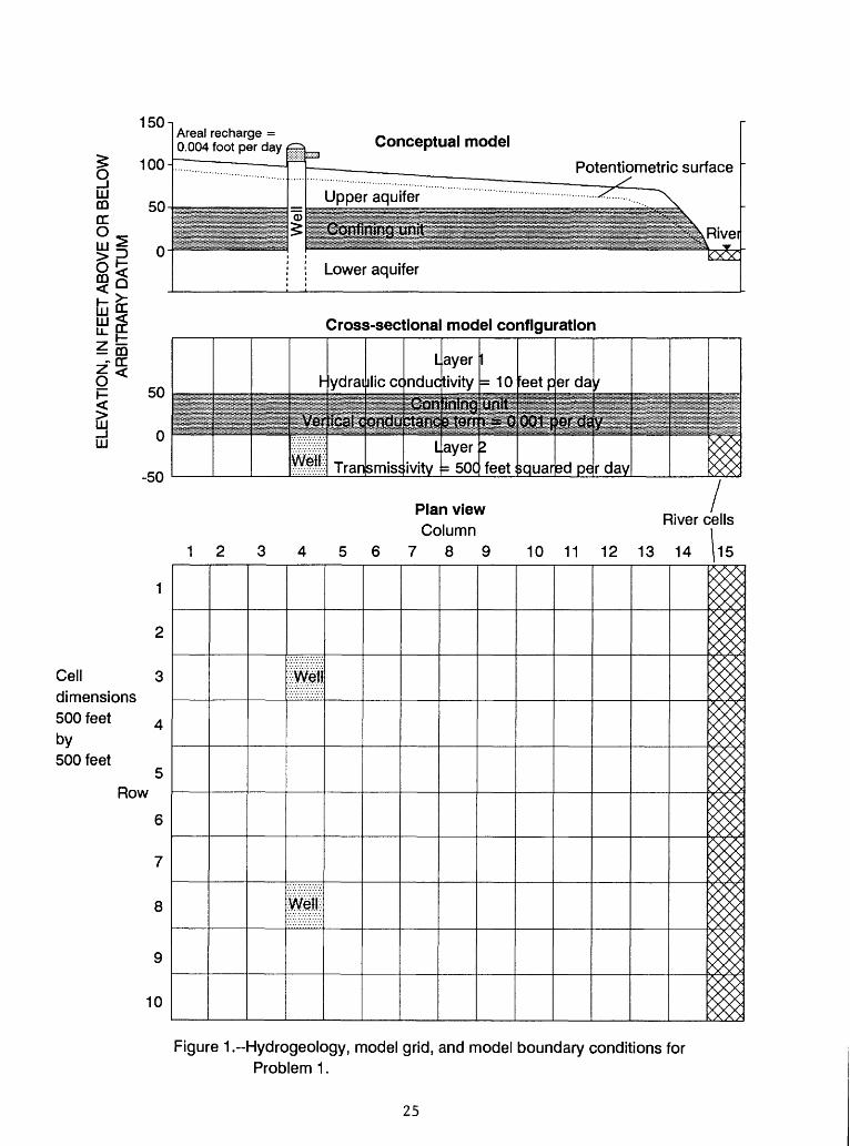
1. Diagram showing hydrogeology, model grid, and model boundaryconditions for Problem 1. ..................... 25
2. Diagram showing hydrogeology, model grid, and model boundaryconditions for Problem 2...................... 40
3. Hydrograph showing simulated head profiles beneath a leaking pond after 190 days, 708 days, 2,630 days, and at steady-state conditions............................. 43
4. Steady-state head profiles simulated using the BCF2 Package andBCF1 Package. ........................... 48
5. Diagram showing hydrogeology, model grid, and model boundaryconditions for Problem 3. ..................... 50
6. Simulated perched water-table profiles after 53 days, 105 days,189 days, 324 days, and at steady-state conditions. ........ 53
iii

7. Flow chart for module BCF2AL. ................... 598. Flow chart for module BCF2RP. ................... 669. Flow chart for module BCF2AD. ................... 72
10. Flow chart for module BCF2FM. ................... 7611. Flow chart for module SBCF2N. ................... 8512. Flow chart for module SBCF2H. ................... 93
TABLES Table
1. Model output for Problem 1. ........2. Wetting and solver input data for Problem 2 simulations
Page . 28 . 42
CONVERSION FACTORS
Multiply
footfoot per daysquare footcubic footcubic foot per daygallon per minute
0.30480.30480.092900.028320.028323.785
To obtain
metermeter per daysquare metercubic metercubic meter per dayliter per minute
IV
A METHOD OF CONVERTING NO-FLOW CELLS TO VARIABLE-HEAD CELLS
IN THE U.S. GEOLOGICAL SURVEY MODULAR FINITE-DIFFERENCE
GROUND-WATER FLOW MODEL
By
Michael G. McDonald, Arlen W. Harbaugh, Brennon R. Orr,
and Daniel J. Ackerman
ABSTRACT
The U.S. Geological Survey Modular Ground-Water Flow Model, commonly
referred to as MODFLOW, simulates ground-water flow through porous media
using the finite-difference method. The region being modeled is divided
into a grid of cells, and each cell is defined to be either no-flow,
variable-head, or constant-head. The model calculates a value for head at
all variable-head cells whereas head at constant-head cells is specified by
the user. Cells are designated as no-flow cells if they contain impermeable
material or are unsaturated, and accordingly the flow of water is not
simulated in such cells.
As originally published, MODFLOW could simulate the desaturation of
variable-head model cells, which resulted in their conversion to no-flow
cells, but could not simulate the resaturation of cells. That is, a no-flow
cell could not be converted to variable head. However, such conversion is
desirable in many situations. For example, one might wish to simulate
pumping that desaturates some cells followed by the recovery of water levels
after pumping is stopped. An option that allows cells to convert from no-
flow to variable-head has been added to the model. In this option, a cell
is converted to variable head based on the head at neighboring cells. The
option is written in FORTRAN 77 and is fully compatible with the existing
model. This report documents the new option, including a description of the
concepts, detailed input instructions, and a listing of the code. Example
problems illustrate the practical applications of the option. Although
solution of the modified flow equations can be difficult for the model
solvers, the example problems show that it is possible to solve a variety of
complex problems.
INTRODUCTION
The U.S. Geological Survey developed a three-dimensional finite-
difference ground-water flow model (McDonald and Harbaugh, 1988) commonly
known as MODFLOW. In the model, the continuous derivatives in the ground-
water flow equation are replaced with finite-difference approximations at
points called nodes. Surrounding each node is a cell in which the hydraulic
properties, such as hydraulic conductivity and storage coefficient, are
defined. The result is a set of N equations containing N values of unknown
head, where N is the number of nodes. The time derivative is approximated
by the backward difference method (McDonald and Harbaugh, 1988, p. 2-16).
The program solves for unknown head at each node at the end of each time
interval.
The finite-difference flow equation for a model cell (i,j,k), where i,
j, and k are row, column, and layer grid indexes respectively (McDonald and
Harbaugh, 1988, p. 2-26), is:
t» v . . , , n _ . , , T (_<L< .. . , n. . _ . , T (_<K. . . , . n.
+ (- cv - -i i. - CC, . . . - CR
- CR. . , . - CC. , . . - CV. . . . + HCOF. . . )hm
-f CR. . . . hm . . . -f CC. . . . hm . . . -f CV. .
- RHS. ... (1) i,J,k
Hydraulic head is designated by h. The equation is written for each
time step in a simulation, and the m superscript designates the time step
number. The HCOF and RHS coefficients incorporate storage and external
stress terms. The CR, CC, and CV coefficients are conductances. Conduct
ance is a combination of several parameters from Darcy's law describing one-
dimensional, steady-state flow occurring in a volume of porous material.
Darcy's law states that flow through a block of porous material is the
product of conductance and the head difference along the flow path. The
terms in equation (1) involving conductance specify the flow between the
node for which the equation is being written and its six neighboring nodes.
A model cell can be one of three types: constant-head, variable-head,
and no-flow. A variable-head cell is one in which the head varies and for
which an equation is formulated. A constant-head cell is one for which,
because the head is known and constant, an equation in terms of the head is
not needed. However, the flow equation for a variable-head cell adjacent to
a constant-head cell contains terms representing flow to or from the
constant-head cell. A no-flow cell is one that represents a portion of the
region in which there can be no movement of water. Such cells either
contain impermeable material or are unsaturated. At no-flow cells, no
equation is formulated, and the flow equation for a variable-head cell
adjacent to a no-flow cell does not contain terms representing flow from the
no-flow cell. The user initially defines a type for each cell by assigning
values to the model array, IBOUND.
As part of the simulation of unconfined aquifers and aquifers that can
convert between confined and unconfined, MODFLOW can change a variable-head
cell to a no-flow cell. The conductance of unconfined cells and cells that
can convert between confined and unconfined depends on the saturated thick
ness, and MODFLOW calculates the saturated thickness for these cells
throughout the simulation. If the saturated thickness becomes zero, MODFLOW
converts the cell to no flow (McDonald and Harbaugh, 1988, p. 5-10). This
conversion is termed "drying" the cell.
The original MODFLOW does not allow a cell to be converted from no flow
to variable head, which is termed "wetting" a cell. A new option to allow
wetting of cells has been added to MODFLOW. Based on head in surrounding
cells, the new model option will attempt to wet cells that are dry. The
user can specify the cells for which wetting is attempted.
There are numerous situations for which the wetting capability is
useful. An example is the recovery of water levels when wells are turned
off. Another example is the mounding that can occur when irrigation is
applied to the surface above an aquifer; the mound could rise into a
previously dry model layer. The wetting capability also is useful in
situations where cells incorrectly go dry (convert to no flow) as part of
the iterative solution process. During the solution process, heads may
temporarily decrease to less than their final values, which may cause cells
to go dry. The new wetting capability allows such cells to convert back to
wet.
MODFLOW was designed in a modular fashion so that it would be easy to
modify (McDonald and Harbaugh, 1988, p. 1-2). The program code was divided
into modules, and the modules were grouped by function into packages. All
modules dealing with internal aquifer flow, which includes flow between
cells and flow into storage, are grouped into a package called the Block-
Centered Flow (BCF) Package. To allow for future revision, each package was
given a version number. The BCF Package documented by McDonald and Harbaugh
(1988) is version 1 and is designated BCF1. The new wetting option was
implemented by creating a replacement package for BCF1. The new package is
BCF version 2, or BCF2. BCF2 is similar to BCF1; many of the modules are
unchanged. All of the previous functionality is provided in addition to the
new wetting capability. BCF2 is written in the FORTRAN 77 programming
language (American National Standards Institute, 1978).
The remainder of this report describes the implementation of the BCF2
Package and how to use it. Several example problems are provided to
illustrate its use. This report is intended to be used as a supplement to
McDonald and Harbaugh (1988).
CONCEPTUALIZATION AND IMPLEMENTATION
The BCF2 Package is identical to the BCF1 Package except for the
wetting and drying of cells. In particular, the BCF2 Package calculates
vertical and horizontal conductance, storage terms, and vertical flow
through a partially saturated zone exactly as done by the BCF1 Package
(McDonald and Harbaugh, 1988, Ch. 5). Accordingly, this report discusses
only the wetting and drying of cells.

For cells that are unconfined or can potentially become unconfined, the
BCF1 Package calculates transmissivity as the product of hydraulic conduc
tivity and saturated thickness. In equation form, transmissivity, TR, is
calculated as (McDonald and Harbaugh, 1988, p. 5-9):
TR - (TOP - EOT) HY for h > TOP (2a)
TR - (h - BOT) HY for TOP > h > BOT (2b)
TR - 0 for h < BOT (2c)
where
HY is the hydraulic conductivity of a cell,
TOP is the elevation of the top of the cell, and
BOT is the elevation of the bottom of the cell.
The transmissivity values for cells are then used to calculate conduct
ances (CR and CC) between cells as required for equation (1). Note that if
horizontal anisotropy exists, hydraulic conductivity, and thus transmissivi
ty, will be different in the row and column directions. Although transmiss
ivity varies with saturated thickness, vertical conductance is a constant
until a cell becomes dry, at which point vertical conductance is changed to
zero.
As defined by equation (2), the value of head is part of the calcula
tion of transmissivity. The head is unknown, however, until equation (1) is
solved. To resolve this conflict, McDonald and Harbaugh (1988) take
advantage of the fact that iterative solvers are used to solve the equations
for head at each cell. Iterative solvers successively improve an approxima
tion of the correct solution until the approximation is sufficiently
accurate. Each approximation is called an iteration, and the solver is said
to converge toward the correct answer. When calculating transmissivity
according to equation (2) for a new iteration, the head from the previous

iteration is used. As the solver converges toward an acceptable solution,
the head from the previous iteration will be nearly equal to the head for
the new iteration. Thus, if all works well, the transmissivity will be
accurate by the time convergence is reached.
In BCF1, a cell becomes dry whenever transmissivity as defined by
equation (2c) is zero. That is, a cell becomes dry when head is below the
bottom elevation. When a cell becomes dry, IBOUND is set to 0 (which
indicates no flow), all conductances to the cell are set to zero, and head
is set to a large value so it will serve as a visual indicator of the
conversion in printouts. The conversion is irreversible in BCF1. BCF2 is
identical to BCF1, except that cells can be wetted.
In BCF2, a dry cell can become wet if the head from the previous
iteration in a neighboring cell is greater than or equal to the turn-on
threshold. The turn-on threshold is
TURNON - BOT + THRESH
where
THRESH is a user-specified constant called the wetting threshold.
The user has two options to select which neighboring cells are checked
to see if the turn-on threshold has been reached. One option is to check
the cell immediately below the dry cell and the four horizontally adjacent
cells. The second option is to check only the cell immediately below the
dry cell. This option is useful when there are relatively large head
differences between adjacent horizontal cells, which means that head in a
neighboring horizontal cell is a poor indicator of when a cell should become
wet.
Only variable-head cells either immediately below or horizontally
adjacent to a dry cell can cause the cell to become wet. That is, if the
neighboring cell is either no flow or constant head, then that cell is not
checked to see if the turn-on threshold has been reached. The reason for
excluding constant-head cells from causing a dry cell to become wet is to
avoid unnecessarily repeating the evaluations of whether a dry cell should
become wet. If the head in a constant-head cell is high enough to cause a
neighboring cell to be wet, then this neighboring cell should be wet during
the entire simulation. The user can make this determination prior to
running the model and can define the cell to be either wet or dry as
appropriate.
When a cell is wetted, IBOUND for the cell is set to 1 (which indicates
a variable-head cell), vertical conductances are set to their original
values, and head at the cell is set either to
h = BOT + WETFCT (hn - BOT) (3a)
or
BOT + WETFCT (THRESH) (3b)
where
hn is the head at the neighboring cell that causes the cell to wet, and
WETFCT is a user-specified constant called the wetting factor.
The user must select between equations (3a) and (3b); the rationale for
making a selection will be discussed later in this report.
Although the head that is assigned to a cell that becomes wet might
exceed the wetting threshold for a neighboring cell, a neighboring cell
cannot become wet as a result of a cell that has become wet in the same
iteration. If this were allowed, a single wetted cell might cause the
entire model to become wet in one iteration.
Once a cell becomes wet, transmissivity and horizontal conductances are
calculated as they are for any variable-head cell, which is the same as done
in the BCF1 Package. The head in a wetted cell will then be recalculated in
subsequent iterations and time steps according to equation (1). A wetted
cell can become dry again.
In transient simulations, the head from the previous time step, HOLD,
is a part of the storage calculation (McDonald and Harbaugh, 1988, p. 5-24).
For cells that become wet after becoming dry in an earlier time step, the
value of HOLD that will produce the correct flow to storage is the bottom
elevation. As a fundamental part of the finite-difference method for
simulating the time derivative in the ground-water flow equation, MODFLOW
begins each time step by setting HOLD equal to head from the end of the
previous time step (McDonald and Harbaugh, 1988, pp. 2-16 and 3-2). Because
the value for head at dry cells is set to a user-specified value when a cell
becomes dry, the BCF2 Package must set HOLD equal to the bottom elevation at
the beginning of each time step for dry cells that have the potential to
become wet. To do this, a new module named BCF2AD has been added to the BCF
Package.
The user should be aware of the possibility that non-unique solutions
can result from the method used to wet cells. Consider a steady-state
problem in which two simulations are made--the first simulation has starting
heads below the final values and the second has starting heads above the
final values. Heads in the first simulation may rise above the bottom of
some dry cells and yet remain below the turn-on threshold. These cells
would remain dry. In the second simulation, head may stay above the bottom
in these same cells, so they would stay wet. Thus, there would be more
variable-head cells in the second simulation even though both simulations
satisfy the prescribed conditions for wetting and drying cells.
PROBLEMS WITH SOLVER CONVERGENCE
The method of wetting and drying cells can cause problems with the
convergence of the iterative solvers used in MODFLOW. Convergence problems
can occur in MODFLOW even without the wetting capability, but problems are
more likely to occur when the wetting capability is used. Symptoms of a
problem are slow convergence or divergence combined with the frequent
wetting and drying of the same cells. It is normal for the same cell to
convert between wet and dry several times during the convergence process,
but frequent conversions are an indication of problems. The user can detect
this situation by examining the model printout; a message is printed each
time a cell converts.
The convergence problems result from several factors. The primary
factor is that equations (1) and (2) together form a nonlinear set of
equations, but they are being solved through the use of solvers designed to
solve linear equations. In particular, if the head from the previous
iteration is poor, then the determination of which cells are wet and dry and
the transmissivity of the wet cells will be incorrect. The overall change
to the system of simultaneous equations that occurs when many cells change
between wet and dry can be another cause of instability. The solvers
perform differently depending on how many equations are being solved and on
the values for conductances in each equation; the wetting and drying process
changes both of these.
Another cause for instability is inaccuracy in the determination of
when cells should become wet. While it is logical that the head at
neighboring cells is a good qualitative indicator of when to wet a cell,
there is no guarantee that a cell that is wetted by the described
methodology should actually be wet. That is, the decision to make a cell
wet should be viewed as a tentative decision. Subsequent iterations will
show if the decision is correct. If head in a wetted cell drops below its
bottom elevation, the cell will become dry again. It is possible for a cell
to repeatedly cycle between wet and dry.
A poor estimate of initial head at wetted cells can also cause
instability. Although the initial head estimate does not impact the final
answer provided that convergence is reached, poor estimates can slow or
prevent convergence by causing incorrect heads to be calculated at nearby
cells.
The user of BCF2 has a number of ways to control solution instability.
1. The user specifies individual cells for which the wetting
capability is active (see parameter WETDRY in "Input Instructions"
section), which makes it possible to avoid the possibility of
wetting dry cells that the user knows should never become wet.
2. The user specifies the wetting threshold for each wettable cell and
which neighboring cells are checked to see if the wetting threshold
has been reached (see parameter WETDRY in "Input Instructions"
section).
3. The choice between using equation 3a or 3b to define the initial
estimate of head at wetted cells is specified by the user.
4. The wetting factor used in 3a and 3b is specified by the user.
5. In steady-state simulations, initial conditions can be adjusted to
improve stability.
For cells that can become wet, the most influential factors for
controlling instability are the wetting threshold and the choice of which
neighboring cells are checked to determine if the wetting threshold has been
reached. The higher the threshold, the more stable the solution.
Unfortunately, the wetting threshold can have a significant impact on the
accuracy of the solution; the higher the wetting threshold, the less
accurate the solution because cells that should become wet might stay dry.
Thus the user may have to make a tradeoff between accuracy and stability.
The choice between equation (3a) and (3b) to define the initial head at
wetted cells can impact solution stability. Equation (3a) is thought to be
the most realistic because it varies the estimate of the head at a wetted
cell according to the head at the cell that causes the cell to become wet.
Equation (3b) bases its estimate of initial head on the wetting threshold.
Equation (3a) can promote instability, however, when the iterative solvers
are generally calculating head changes that are higher than optimum. In
10
that situation, equation (3b) can have a stabilizing effect. Both equations
also include the wetting factor, WETFCT, which can be used to increase or
decrease the estimate of head at a wetted cell.
Adjustments of the wetting threshold, the choice between equations (3a)
and (3b), and wetting factor must be made on a trial and error basis. After
adjusting any of these, the user should examine the output to see if a
stable solution has been obtained and if acceptable determinations of which
cells are wet and dry have been made.
For steady-state simulations, benefit can be gained by making an effort
to set initial conditions as close as possible to final conditions. Of
course the final heads are not known prior to running the simulation because
the purpose of running a simulation is to solve for heads; however, it is
often possible to make a good estimate of final heads. By using good
estimates of initial head and the boundary array (IBOUND), which indicates
which cells initially are wet and dry, conversions of cells between wet and
dry can be minimized. Note that for transient simulations, there is no
flexibility to adjust initial conditions; initial conditions must be set to
accurately reflect conditions at the start of the simulation.
Up to this point, it has been implied that the wetting of cells is
tested for at the start of every iteration. Although performing this test
every iteration would appear to promote the most rapid solution, solution
speed can sometimes be improved by limiting the iterations at which the
wetting can occur. The reason is that the wetting of cells sometimes
produces erroneous head changes in neighboring cells during the succeeding
iteration, which would cause erroneous conversions of those cells. These
erroneous conversions can be prevented by waiting a few iterations until
heads have had a chance to adjust before testing for additional conversions.
Accordingly, the ability to specify when wetting can be attempted has been
incorporated into BCF2. In particular, the user can specify the iteration
interval, IWETIT, for attempting to wet cells. That is, every IWETIT
iterations starting from the beginning of each time step, BCF2 attempts to
wet cells. At iterations for which no wetting is allowed, cells may still
convert to dry. When setting IWETIT greater than one, there is some risk
11

that cells may be prevented from correctly converting to wet. If the
solution for a time step is obtained in less than IWETIT iterations, then
there will be no check during that time step to see if cells should convert
to wet. The potential for this problem is greatest in transient
simulations, which frequently require only a few iterations for a time step.
The last way for controlling oscillation is through the choice of the
solver and adjustments of that solver. Three methods of iterative solution
are available for MODFLOW. The Slice-Successive Overrelaxation (SOR) method
(McDonald and Harbaugh, 1988, Ch. 13), the Strongly Implicit Procedure (SIP)
method (McDonald and Harbaugh, 1988, Ch. 12), and the the Preconditioned
Conjugate-Gradient (PCG) method (Kuiper, 1987, and Hill, 1990). SIP and PCG
have been used successfully with BCF2. PCG appears to be the best. The SOR
method is generally not practical for use with BCF2. Each solver
implementation has input parameters that can affect the convergence
efficiency. The reader should refer to the documentation of the solvers for
specific information on the ways to adjust them.
Users of the PCG solvers should be aware that both of these solvers
make use of a dual-iteration methodology, which can be useful in controlling
oscillation of cells between wet and dry. Hill (1990) describes the
iteration methodology using the terms "inner" and "outer" iterations. An
outer iteration is a model iteration as described by McDonald and Harbaugh
(1988, p. 2-20). For each outer iteration, the PCG solver can perform
multiple iterations, called inner iterations. During successive inner
iterations, PCG improves the calculated head assuming that all parameters in
the flow equation are constant. In particular, cells cannot change between
wet and dry during inner iterations. Thus, PCG's inner iterations serve a
similar purpose to that of the IWETIT iteration interval, and generally
there is no need to use an IWETIT value other than 1 when using PCG. Note
that IWETIT applies to outer iterations in PCG; the BCF2 Package has no
control over inner iterations. Note also that the BCF2 iteration interval
controls only the wetting of cells and does not have an impact on the other
head-dependent formulations such as transmissivity and the resulting
conductances within the BCF2 Package or any other model package. No head-
dependent formulations occur in any packages during PCG inner iterations.
12
In an unstable problem in which many cells are erratically converting
between wet and dry, the solvers can have numerical problems that cause them
to abort. In particular, small clusters of cells isolated from the rest of
the cells by no-flow cells can cause division by zero in the solvers. In
addition, the PCG2 solver (Hill, 1990) may calculate a Cholesky matrix that
is not diagonally dominant, which will cause the solver to abort. In some
cases setting the value of PCG2 parameter RELAX in the range of 0.97 to 0.99
prevents zero divide and non-diagonally dominant matrix errors.
APPLICABILITY AND LIMITATIONS
The BCF2 Package makes it possible to simulate situations in which a
water table rises into unsaturated model layers. A typical application of
this capability is in the simulation of the recovery of over-stressed
aquifers either through artificial recharge or the reduction of stress. The
need for the wetting capability increases as the need for vertical detail of
head distribution increases. High-accuracy simulations of vertical head
gradients are required for such purposes as tracking the flow of contami
nants, especially when significant vertical heterogeneity exists or when
stresses partially penetrate an aquifer. To obtain accuracy of vertical
head requires many model layers, which implies that each layer will be thin.
The thinner the model layer, the more likely it is that cells will require
conversions between wet and dry.
Another benefit of the wetting capability is improved simulation of
declining water tables. Although the BCF1 Package can simulate the drying
of cells when water levels decrease, there is a risk of drying cells that
should not become dry. This can happen when an iterative solver overshoots
the correct value during an iteration, which is not unusual for iterative
solvers. The wetting capability of BCF2 allows such cells to become wet
again in later iterations.
Although the BCF2 Package has the ability to simulate a variety of
situations, there are limitations to its use. The primary limitation has
already been discussed; there may be instabilities in the solution process
13
that prevent solution or cause solution to require excessive computational
time. To minimize solution problems, the user can choose from the SIP and
PCG solvers, can adjust the solvers, and can adjust the data that controls
the wetting process. All of the adjustments must be done through trial and
error. Once a solver produces an answer, the user must examine the results
to determine if the answer is acceptable. The budget error should be
examined as well as which cells are wet and dry. Although the wetting
threshold might have to be higher than one would like, the answers produced
are probably more accurate than would otherwise be produced without the
wetting capability.
A second limitation of BCF2 results from the method of drying cells.
All stresses are removed when a cell becomes dry even though it might be
more appropriate to move the stress to another location. For example, if a
cell that contains a well goes dry, the pumpage will be eliminated. If the
well owner would likely deepen the well rather than stop pumping water, a
more appropriate action would be to move the pumpage to a deeper cell.
Further, the removal of stresses when cells go dry can cause cells to
repeatedly convert between wet and dry. In the example of a drying cell
that contains a well, the elimination of the pumpage might then allow the
cell to become wet again; this cycle could repeat indefinitely. Note that
the Recharge (RCH) Package (McDonald and Harbaugh, 1988, Ch. 7) has an
option to deal with this problem; it can allow recharge to pass through dry
cells to the highest constant-head or variable-head cell. Likewise, this
capability of the Recharge Package could be used to simulate wells whose
pumpage is automatically moved to the next lower layer when a layer goes
dry. Some situations may require new methods for simulating stresses; the
modular design of MODFLOW makes it possible to easily add new capabilities.
A similar problem can result in transient simulations, which involve
flow from storage. If a cell dries, the flow from storage at that time step
is lost. Large volumes of water could be lost, causing an inaccurate
simulation. For example, it is possible to specify large time steps such
that the head in a cell drops from the top of the cell to the bottom in one
time step. In this situation, all of the unconfined storage, which is
generally a large quantity, would be lost. The solution to this problem is
14
to use time steps that are small enough to allow most of a cell's water to
be taken from storage before the cell converts to dry. However, small time
steps can cause additional problems. Small time steps result in large rates
of flow from storage when a cell becomes wet because flow from storage is
dependent on the inverse of time-step length. The flow to storage can
result in head in the wetted cell being only slightly above the bottom of
the cell. The small saturated thickness results in a low transmissivity
that can restrict the flow entering the cell from adjacent cells enough to
cause the cell to convert to dry again. Also, the large flow to storage
caused by wetting a cell can cause the solvers to over-compensate and reduce
head enough to dry the cell. Thus, small time steps can result in repeated
conversions between wet and dry. If small time steps are required, a larger
wetting threshold may be necessary to avoid the oscillation between wet and
dry.
A third limitation is the way vertical conductance converts when a cell
changes between dry and wet. When dry, conductance is zero; when wet,
conductance is a constant. If a confining layer exists between layers as
assumed by McDonald and Harbaugh (1988, p. 5-30), this makes sense. That
is, if the confining bed is the primary restriction to vertical flow, then
the lowering of the water table in the aquifer above the confining unit will
not change the vertical conductance very much because the confining unit is
not changed by the aquifer's desaturation. When there is no confining layer
as would be the situation when a single aquifer is being simulated by
multiple model layers, the changing water level would have a significant
impact on vertical conductance. A more accurate representation would be to
vary vertical conductance with saturated thickness. To reduce the error,
more layers can be used.
Another limitation also involves vertical flow. Vertical flow between
two cells is limited when the lower cell is not confined (McDonald and
Harbaugh, 1988, p. 5-19). This is appropriate for simulating perched
conditions that can occur when there is recharge to the upper cell and there
is a low-conductivity material between the two cells or the upper cell has
lower hydraulic conductivity than the lower cell. A stress in the lower
cell can cause the head to drop below the top without drying the upper cell.
15
When vertical flow is limited, vertical flow is calculated as saturated
thickness of the upper cell times the vertical conductance. Thus, flow is
not dependent on the head in the lower cell. A problem can occur if flow is
limited between two cells that are simulating the same aquifer. That is, it
is possible for a perched water table to form in the model when heads are
declining even though there is no low conductivity material between the
cells that could cause the perched condition. Although this would not
happen if model heads were declining smoothly from the top down, it can
happen if heads in a lower cell drop below its top during the iterative
convergence process while the cell above is still wet. Once the perched
condition is established, it can stay even though it does not make
hydrologic sense because the vertical flow limitation prevents head from
dropping as low as it should drop. Thus the user should examine model heads
to see if there are cells having incorrectly perched conditions.
The final limitation involves the difficulty of preparing data for the
BCF2 Package. The user is faced with a major effort to prepare the input
data for a typical multi-layer problem that requires the wetting capability.
Errors are a likelihood given the amount of data, and errors probably will
be difficult to trace. Inconsistent top and bottom elevations and other
incorrect data can cause convergence problems in addition to the convergence
problems that are inherent in the model formulations. When faced with a
model that will not converge, it is difficult to determine whether there is
a fundamental stability problem or bad data somewhere in the input files.
It is often helpful to make a series of increasingly complex models rather
than starting off with the "full-blown" model. For example, a complex
water-table aquifer system might be simulated initially as a single
unconfined aquifer even though the final model will simulate the aquifer
with a sequence of model layers, some of which will use the wetting
capability. This makes it possible to get the basic model operational and
obtain some knowledge of the values for aquifer parameters before dealing
with the problems of the wetting and drying of cells.
16
INPUT INSTRUCTIONS
Most of the data required by the BCF2 Package are the same as for the
BCF1 Package. These data consist primarily of arrays that are used to
calculate conductance and storage terms for each layer. The required arrays
can include transmissivity, hydraulic conductivity, specific yield, confined
storage coefficient, vertical leakance, aquifer bottom elevation, and
aquifer top elevation. The specific arrays required depend on the options
that are used as indicated by the layer-type code, LAYCON. The reader is
referred to McDonald and Harbaugh (1988, p. 5-30) for a detailed description
of these data.
A small amount of data is required for the wetting capability in
addition to that required by the BCFl Package. The additional data are a
flag indicating if the wetting capability is to be used, the wetting
threshold, the wetting factor, and the iteration interval for attempting to
wet cells. The only additional array is WETDRY, which must be specified for
each wettable layer. If the wetting capability is enabled, all layers for
which transmissivity varies with saturated thickness, which is indicated by
a LAYCON value of 1 or 3, are wettable.
Because BCF2 is designed as a replacement for BCFl, input is read using
the same unit number, which is specified in IUNIT(1). Refer to McDonald and
Harbaugh (1988, p. 3-25) for a description of the use of unit numbers in
MODFLOW. The data must be in the specified order. The data are read once
at the start of the simulation.
BCF2AL
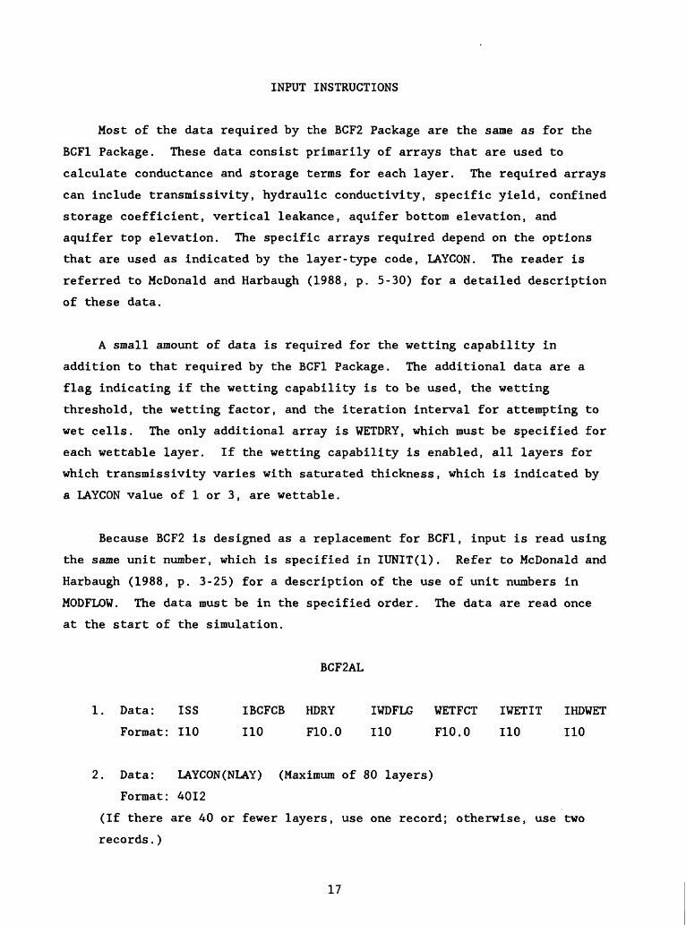
1. Data: ISS IBCFCB HDRY IWDFLG WETFCT IWETIT IHDWET
Format: 110 110 F10.0 110 F10.0 110 110
2. Data: LAYCON(NLAY) (Maximum of 80 layers)
Format: 4012
(If there are 40 or fewer layers, use one record; otherwise, use two
records.)
17
BCF2RP
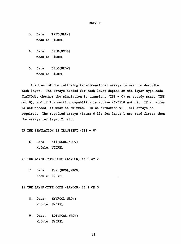
3. Data: TRPY(NLAY)
Module: U1DREL
4. Data: DELR(NCOL)
Module: U1DREL
5. Data: DELC(NROW)
Module: U1DREL
A subset of the following two-dimensional arrays is used to describe
each layer. The arrays needed for each layer depend on the layer-type code
(LAYCON), whether the simulation is transient (ISS - 0) or steady state (ISS
not 0), and if the wetting capability is active (IWDFLG not 0). If an array
is not needed, it must be omitted. In no situation will all arrays be
required. The required arrays (items 6-13) for layer 1 are read first; then
the arrays for layer 2, etc.
IF THE SIMULATION IS TRANSIENT (ISS - 0)
6. Data: sfl(NCOL,NROW)
Module: U2DREL
IF THE LAYER-TYPE CODE (LAYCON) is 0 or 2
7. Data: Tran(NCOL.NROW)
Module: U2DREL
IF THE LAYER-TYPE CODE (LAYCON) IS 1 OR 3
8. Data: HY(NCOL.NROW)
Module: U2DREL
9. Data: BOT(NCOL.NROW)
Module: U2DREL
18
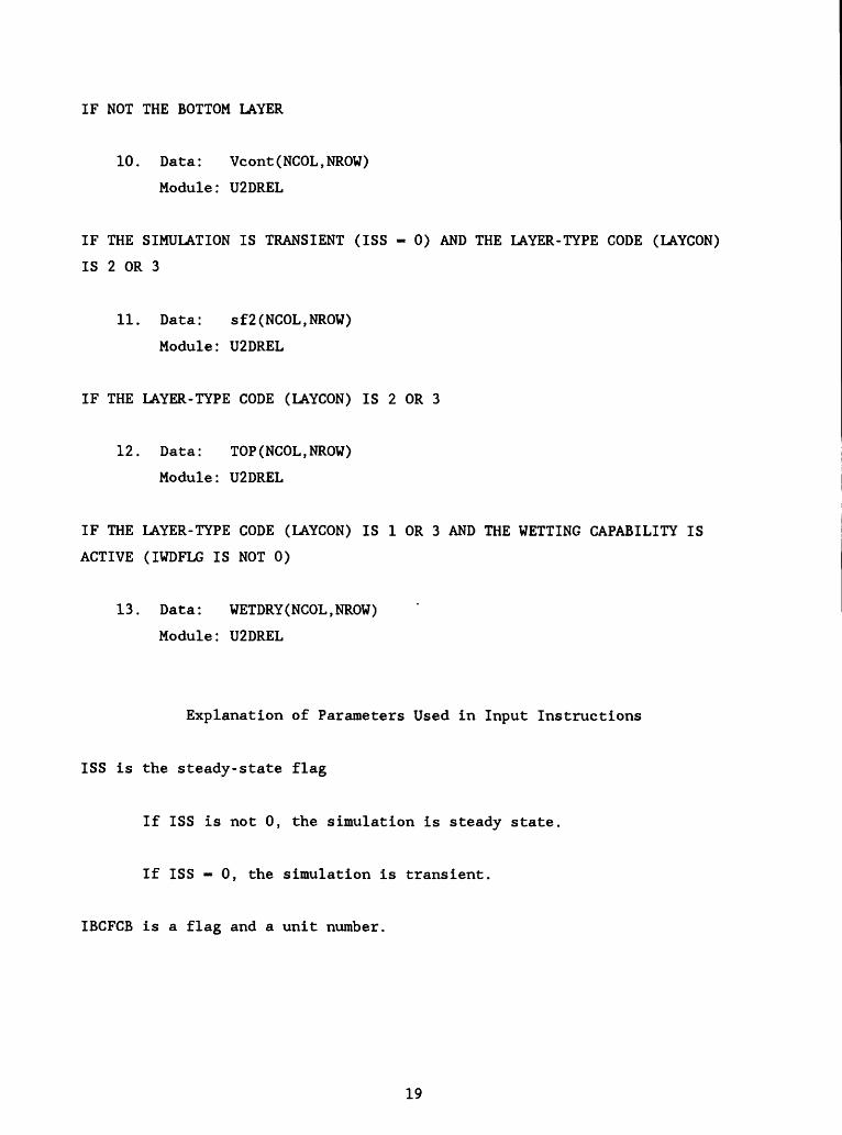
IF NOT THE BOTTOM LAYER
10. Data: Vcont(NCOL.NROW)
Module: U2DREL
IF THE SIMULATION IS TRANSIENT (ISS - 0) AND THE LAYER-TYPE CODE (LAYCON)
IS 2 OR 3
11. Data: sf2(NCOL,NROW)
Module: U2DREL
IF THE LAYER-TYPE CODE (LAYCON) IS 2 OR 3
12. Data: TOP(NCOL.NROW)
Module: U2DREL
IF THE LAYER-TYPE CODE (LAYCON) IS 1 OR 3 AND THE WETTING CAPABILITY IS
ACTIVE (IWDFLG IS NOT 0)
13. Data: WETDRY(NCOL.NROW)
Module: U2DREL
Explanation of Parameters Used in Input Instructions
ISS is the steady-state flag
If ISS is not 0, the simulation is steady state.
If ISS - 0, the simulation is transient.
IBCFCB is a flag and a unit number.
19
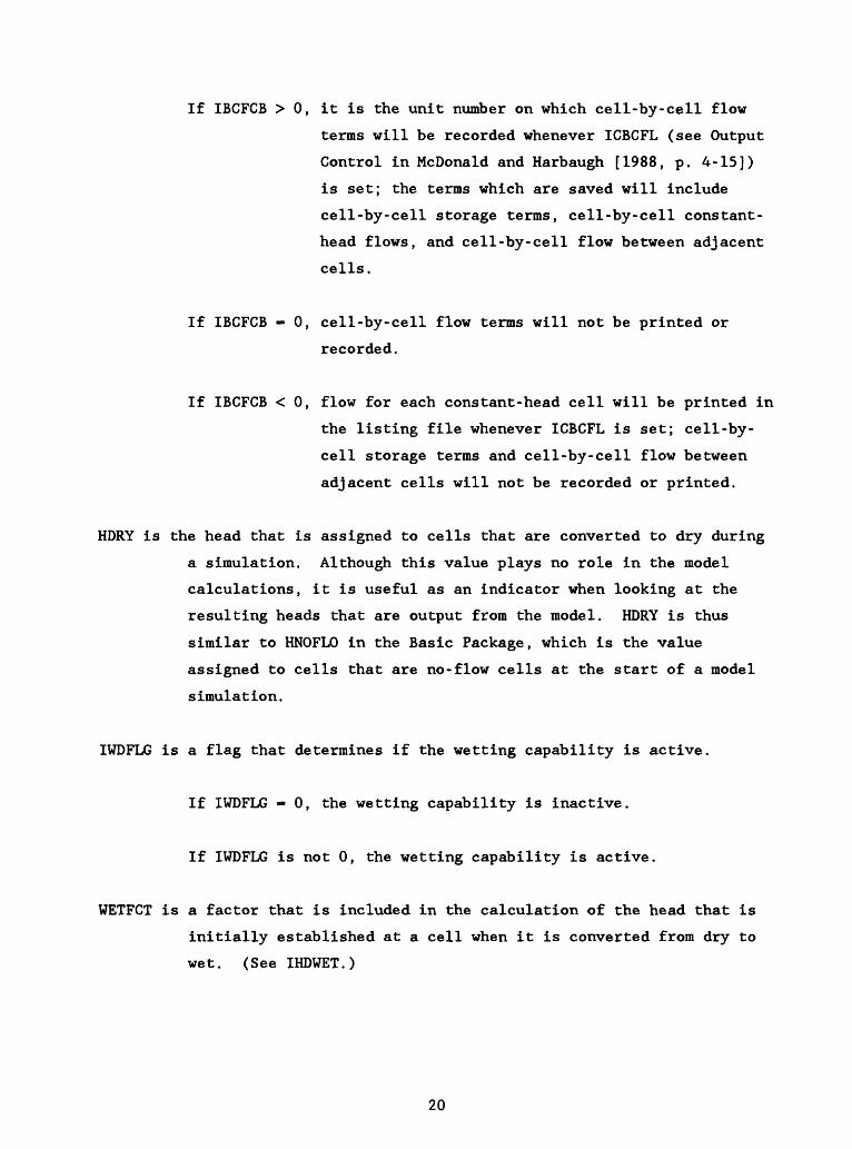
If IBCFCB > 0, it is the unit number on which cell-by-cell flow
terms will be recorded whenever ICBCFL (see Output
Control in McDonald and Harbaugh [1988, p. 4-15])
is set; the terms which are saved will include
cell-by-cell storage terms, cell-by-cell constant-
head flows, and cell-by-cell flow between adjacent
cells.
If IBCFCB - 0, cell-by-cell flow terms will not be printed or
recorded.
If IBCFCB < 0, flow for each constant-head cell will be printed in
the listing file whenever ICBCFL is set; cell-by-
cell storage terms and cell-by-cell flow between
adjacent cells will not be recorded or printed.
HDRY is the head that is assigned to cells that are converted to dry during
a simulation. Although this value plays no role in the model
calculations, it is useful as an indicator when looking at the
resulting heads that are output from the model. HDRY is thus
similar to HNOFLO in the Basic Package, which is the value
assigned to cells that are no-flow cells at the start of a model
simulation.
IWDFLG is a flag that determines if the wetting capability is active.
If IWDFLG - 0, the wetting capability is inactive.
If IWDFLG is not 0, the wetting capability is active.
WETFCT is a factor that is included in the calculation of the head that is
initially established at a cell when it is converted from dry to
wet. (See IHDWET.)
20
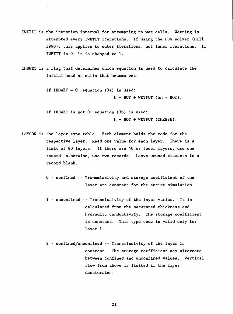
IWETIT is the iteration interval for attempting to wet cells. Wetting is
attempted every IWETIT iterations. If using the PCG solver (Hill,
1990), this applies to outer iterations, not inner iterations. If
IWETIT is 0, it is changed to 1.
IHDWET is a flag that determines which equation is used to calculate the
initial head at cells that become wet:
If IHDWET - 0, equation (3a) is used:
h - EOT + WETFCT (hn - EOT),
If IHDWET is not 0, equation (3b) is used:
h - EOT + WETFCT (THRESH).
LAYCON is the layer-type table. Each element holds the code for the
respective layer. Read one value for each layer. There is a
limit of 80 layers. If there are 40 or fewer layers, use one
record; otherwise, use two records. Leave unused elements in a
record blank.
0 - confined -- Transmissivity and storage coefficient of the
layer are constant for the entire simulation.
1 - unconfined -- Transmissivity of the layer varies. It is
calculated from the saturated thickness and
hydraulic conductivity. The storage coefficient
is constant. This type code is valid only for
layer 1.
2 - confined/unconfined -- Transmissivity of the layer is
constant. The storage coefficient may alternate
between confined and unconfined values. Vertical
flow from above is limited if the layer
desaturates.
21
3 - confined/unconfined -- Transmissivity of the layer varies. It
is calculated from the saturated thickness and
hydraulic conductivity. The storage coefficient
may alternate between confined and unconfined
values. Vertical flow from above is limited if
the aquifer desaturates.
TRPY is a one-dimensional array containing an anisotropy factor for each
layer. It is the ratio of transmissivity or hydraulic conductivity
(whichever is being used) along a column to transmissivity or
hydraulic conductivity along a row. Set to 1.0 for isotropic
conditions. This is a single array with one value per layer. Do
not read an array for each layer; include only one array control
record for the entire array. If the value is the same for all
layers, the entire array can be specified by setting LOCAT to 0 and
setting CNSTNT to the value that applies to all layers.
DELR is the cell width along rows. Read one value for each of the NCOL
columns. This is a single array with one value for each column.
DELC is the cell width along columns. Read one value for each of the NROW
rows. This is a single array with one value for each row.
sfl is the primary storage coefficient. Read only for a transient
simulation (steady-state flag, ISS, is 0). For LAYCON equal to 1,
sfl will always be specific yield, while for LAYCON equal to 2 or 3,
sfl will always be confined storage coefficient. For LAYCON equal to
0, sfl would normally be confined storage coefficient; however, a
LAYCON value of 0 can also be used to simulate water-table conditions
where drawdowns are expected to remain everywhere a small fraction of
the saturated thickness, and where there is no layer above, or flow
from above is negligible. In this case, specific yield values would
be entered for sfl.
22
Tran is the transmissivity along rows. Tran is multiplied by TRPY to obtain
transmissivity along columns. Read only for layers where LAYCON is 0
or 2.
HY is the hydraulic conductivity along rows. HY is multiplied by TRPY to
obtain hydraulic conductivity along columns. Read only for layers
where LAYCON is 1 or 3.
BOT is the elevation of the aquifer bottom. Read only for layers where
LAYCON is 1 or 3.
Vcont is the vertical hydraulic conductivity divided by the thickness from a
layer to the layer below. The value for a cell is the hydraulic
conductivity divided by thickness for the material between the node
in that cell and the node in the cell below. Because there is not a
layer beneath the bottom layer, Vcont cannot be specified for the
bottom layer.
sf2 is the secondary storage coefficient. Read only for layers where LAYCON
is 2 or 3 and only if the simulation is transient (steady-state flag,
ISS, is 0). The secondary storage coefficient is always specific
yield.
TOP is the elevation of the aquifer top. Read only for layers where LAYCON
is 2 or 3.
WETDRY is a combination of the wetting threshold and a flag to indicate
which neighboring cells can cause a cell to become wet. If WETDRY <
0, only the cell below a dry cell can cause the cell to become wet.
If WETDRY > 0, the cell below a dry cell and the four horizontally
adjacent cells can cause a cell to become wet. If WETDRY is 0, the
cell cannot be wetted. The absolute value of WETDRY is the wetting
threshold. When the sum of BOT and the absolute value of WETDRY at a
dry cell is equaled or exceeded by the head at an adjacent cell, the
cell is wetted. Read only if LAYCON is 1 or 3 and IWDFLG is not 0.
23

EXAMPLE PROBLEMS
Example problems were posed to illustrate the practical applications of
the BCF2 option. Although solution of the modified flow equations can be
difficult for the model solvers, the example problems show that it is
possible to solve a variety of complex problems.
Problem 1 -- Simulation of a Two-Laver Aquifer System
in which the Top Layer Converts Between Wet and Dry
In an aquifer system where two aquifers are separated by a confining
bed, large pumpage withdrawals from the bottom aquifer can desaturate parts
of the upper aquifer. If pumpage is discontinued, resaturation of the upper
aquifer can occur. This problem demonstrates the capability of the BCF2
Package to successfully simulate this common hydrologic situation which is
difficult or impossible to simulate with the original BCF1 Package. If both
aquifers were simulated by one model layer using BCFl, the effect of the
confining bed on vertical flow could not be simulated. Also, the trans-
missivity would not be correctly calculated as a function of saturated
thickness. The changes in hydraulic conductivity between the confining bed
and the aquifers could not be distinctly represented. If each aquifer were
simulated by a separate model layer using BCFl, there would be solution
difficulties. When simulating declining heads, too many cells might convert
to dry; when simulating rising heads, dry cells could not convert to wet.
Conceptual Model
A hypothetical aquifer system consists of two aquifers separated by a
confining unit (fig. 1). No-flow boundaries surround the system on all
sides, except that the lower aquifer discharges to a stream along the right
side of the area. Recharge from precipitation is applied evenly over the
entire area. The stream penetrates the lower aquifer; in the region above
the stream, the upper aquifer and confining unit are missing. Under natural
conditions, recharge flows through the system to the stream. Under
24
IHIco cc
si
HI S
ii ^ co^rCC
<
HI
150n
100-
50
0
Areal recharge = 0.004 foot per day
Cell 3 dimensions 500 feet 4 by500 feet
5Row
10
1 2
Conceptual model
_
Upper aquifer
Potentiometric surface
Cross-sectional model configuration
5 6
Plan viewColumn 789
River cells
10 11 12 13 14 15
Figure 1 .-Hydrogeology, model grid, and model boundary conditions for Problem 1.
25
stressed conditions, two wells withdraw water from the lower aquifer. If
enough water is pumped, cells in the upper aquifer will desaturate. Removal
of the stresses will then cause the desaturated areas to resaturate.
Modeling Approach
The model consists of two layers--one for each aquifer. Because
horizontal flow in the confining bed is small compared to horizontal flow in
the aquifers and storage is not a factor in steady-state simulations, the
confining bed is not treated as a separate layer. The effect of the confin
ing bed is incorporated in the value for vertical hydraulic conductivity
divided by thickness between aquifer layers (McDonald and Harbaugh, 1988, p.
5-16). Note that if storage in the confining bed were significant, trans
ient simulations would require that the confining layer be simulated using
one or more layers. A uniform horizontal grid of 10 rows and 15 columns is
used. Aquifer parameters are specified as shown in Figure 1.
Simulation Results
Two steady-state solutions were obtained to simulate natural conditions
and pumping conditions. The two solutions are designed to demonstrate the
ability of the BCF2 Package to handle a broad range of possibilities for
cells converting between wet and dry in the top aquifer. When solving for
natural conditions, the top aquifer initially is specified as being entirely
dry and many cells must convert to wet. When solving for pumping
conditions, the top aquifer is initially specified to be under natural
conditions and many cells must convert to dry.
The steady-state solutions were obtained through a single simulation
consisting of two stress periods. The first stress period simulates natural
conditions and the second period simulates the addition of pumping wells.
The simulation is declared to be steady state, so no storage values are
specified and each stress period requires only a single time step to produce
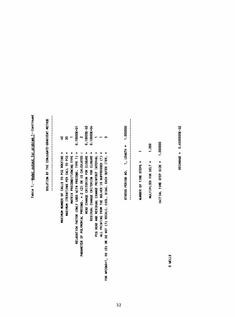
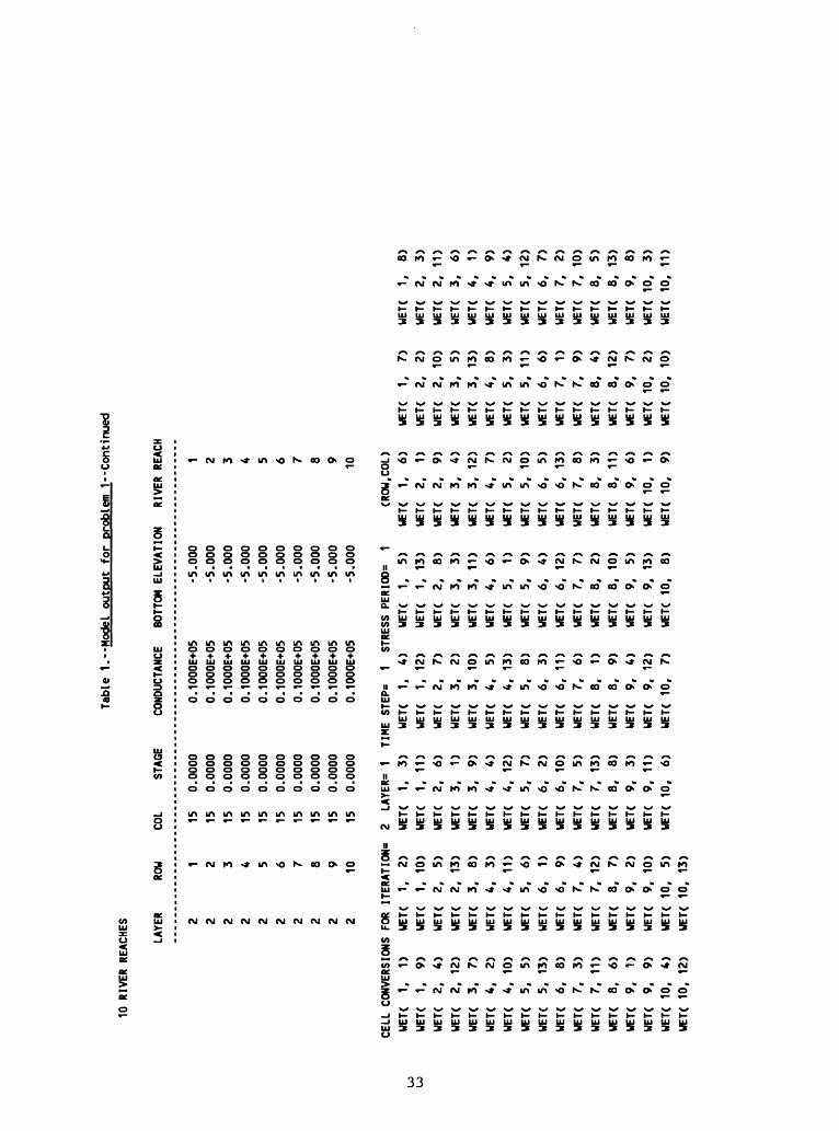
a steady-state result. The PCG2 Package is used to solve the flow equations
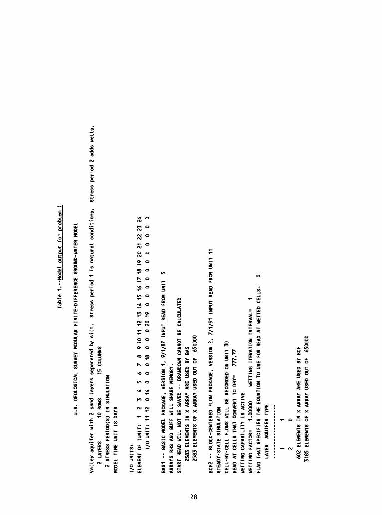
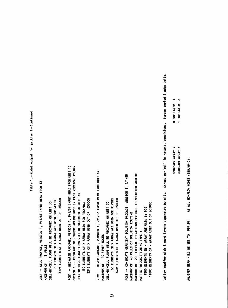
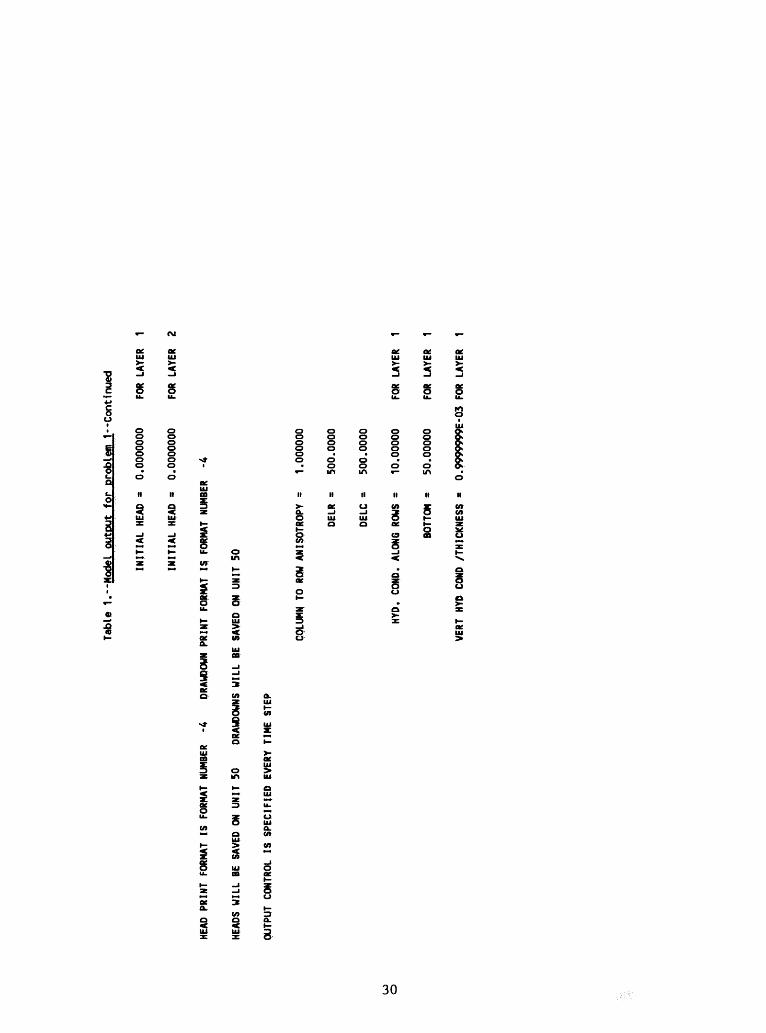
26
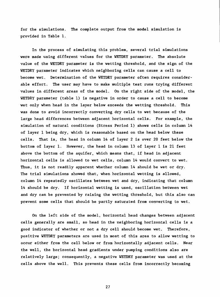
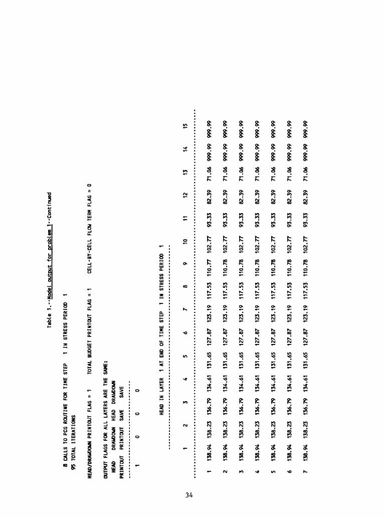
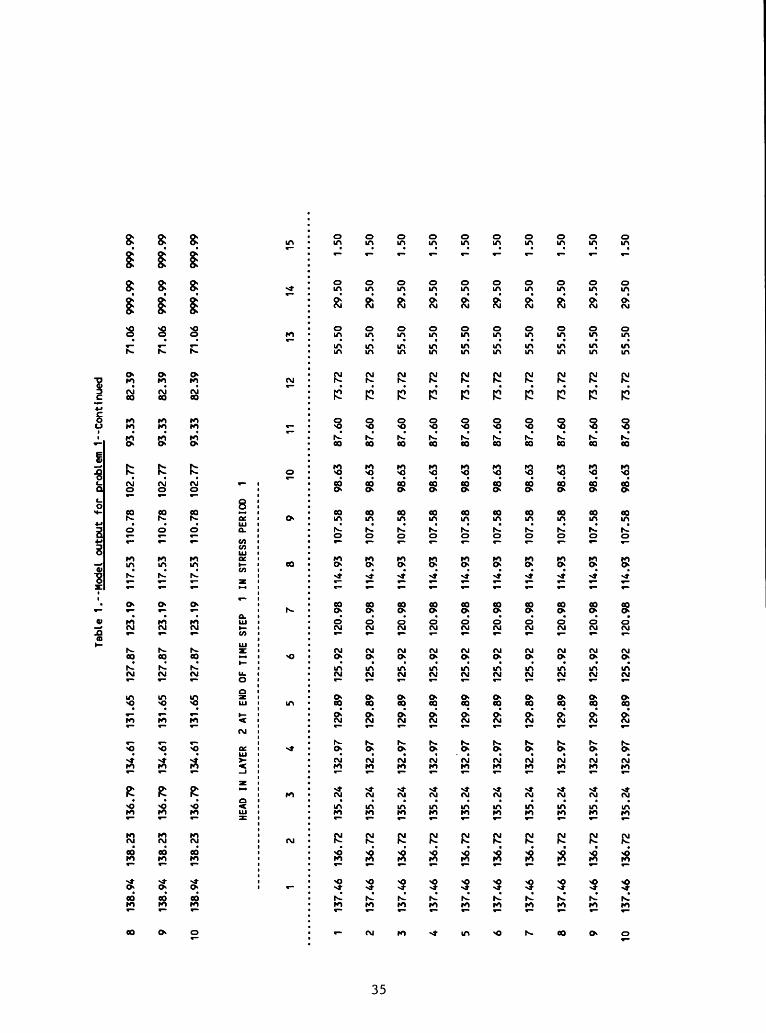
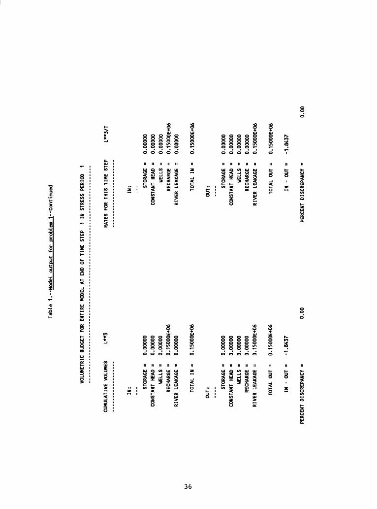
for the simulations. The complete output from the model simulation is
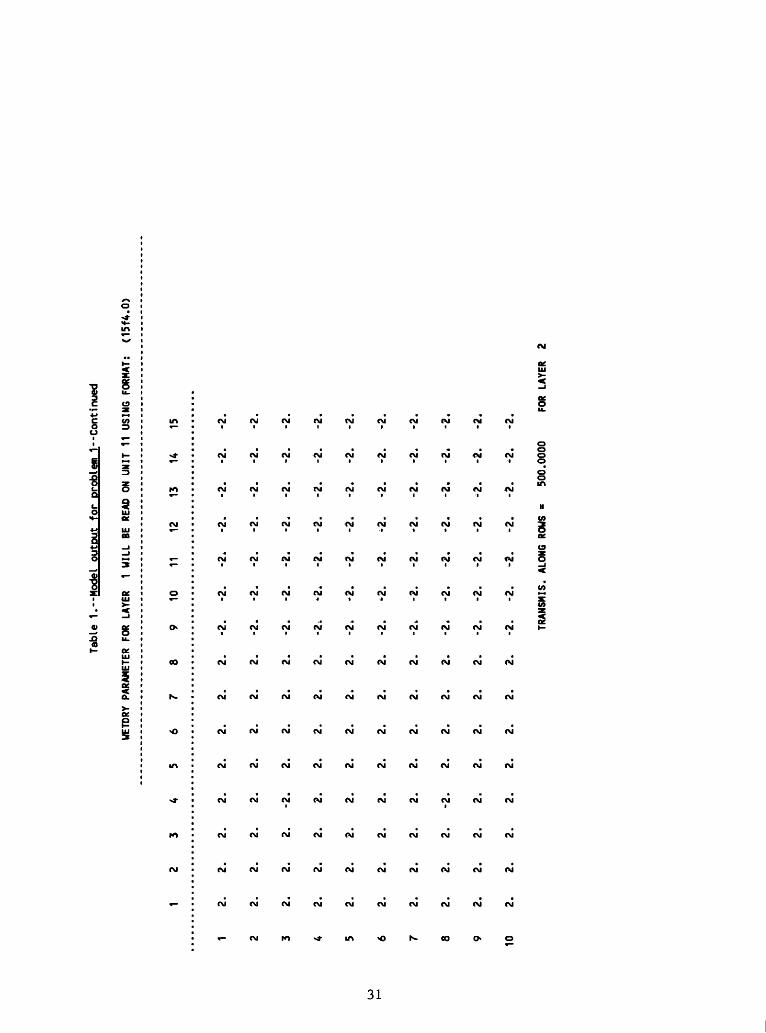
provided in Table 1.
In the process of simulating this problem, several trial simulations
were made using different values for the WETDRY parameter. The absolute
value of the WETDRY parameter is the wetting threshold, and the sign of the
WETDRY parameter indicates which neighboring cells can cause a cell to
become wet. Determination of the WETDRY parameter often requires consider
able effort. The user may have to make multiple test runs trying different
values in different areas of the model. On the right side of the model, the
WETDRY parameter (table 1) is negative in order to cause a cell to become
wet only when head in the layer below exceeds the wetting threshold. This
was done to avoid incorrectly converting dry cells to wet because of the
large head differences between adjacent horizontal cells. For example, the
simulation of natural conditions (Stress Period 1) shows cells in column 14
of layer 1 being dry, which is reasonable based on the head below these
cells. That is, the head in column 14 of layer 2 is over 20 feet below the
bottom of layer 1. However, the head in column 13 of layer 1 is 21 feet
above the bottom of the aquifer, which means that, if head in adjacent
horizontal cells is allowed to wet cells, column 14 would convert to wet.
Thus, it is not readily apparent whether column 14 should be wet or dry.
The trial simulations showed that, when horizontal wetting is allowed,
column 14 repeatedly oscillates between wet and dry, indicating that column
14 should be dry. If horizontal wetting is used, oscillation between wet
and dry can be prevented by raising the wetting threshold, but this also can
prevent some cells that should be partly saturated from converting to wet.
On the left side of the model, horizontal head changes between adjacent
cells generally are small, so head in the neighboring horizontal cells is a
good indicator of whether or not a dry cell should become wet. Therefore,
positive WETDRY parameters are used in most of this area to allow wetting to
occur either from the cell below or from horizontally adjacent cells. Near
the well, the horizontal head gradients under pumping conditions also are
relatively large; consequently, a negative WETDRY parameter was used at the
cells above the well. This prevents these cells from incorrectly becoming
27
Tabl
e 1.
--Mo
del
outp
ut fo
r problem
1
U.S.
GE
OLOG
ICAL
SURVEY MO
DULAR
FINITE-DIFFERENCE
GROU
ND-W
ATER
MODEL
Vall
ey a
quifer w
ith
2 sa
nd la
yers
separated b
y si
lt.
Stre
ss p
erio
d 1
is n
atur
al conditions.
Stre
ss p
erio
d 2
adds w
ells
.2
LAYE
RS
10 R
OWS
15 COLUMNS
2 ST
RESS
PE
RIOD
(S)
IN SIMULATION
MODEL
TIME UN
IT IS D
AYS
I/O
UNITS:
ELEMENT
OF IU
NIT:
1
2 3
4 5
6 78 9
10 11
12 13
14
15
16 17
18
19 2
0 21
22 23 24
I/O
UNIT:
11 12
0 14 000 18 000 20 19
00000000000
BAS1 --
BASIC
MODE
L PACKAGE, VERSION
1, 9/
1/87
INPUT
READ FR
OM U
NIT
5
ARRAYS RHS
AND
BUFF
WI
LL SH
ARE
MEMORY.
STAR
T HEAD W
ILL
NOT
BE SAVED
-- DRAWDOWN C
ANNO
T BE CALCULATED
2583
EL
EMEN
TS IN X AR
RAY
ARE
USED BY BAS
00
2583
EL
EMEN
TS O
F X AR
RAY
USED
OUT
OF
650000
BCF2 -- BLOCK-CE
NTER
ED FLOW PACKAGE, VERSION
2, 7/1/91 IN
PUT
READ FROM U
NIT
11
STEADY-STATE SIMULATION
CELL-BY-CELL FLOWS
WILL BE
RE
CORD
ED O
N UNIT 3
0
HEAD
AT CELLS
THAT
CONVERT
TO D
RY=
777.
77
WETTING
CAPABILITY IS A
CTIV
E
WETTING
FACTOR=
1.00000
WETT
ING
ITER
ATIO
N IN
TERV
AL=
1
FLAG TH
AT SP
ECIF
IES
THE
EQUATION TO
USE
FO
R HEAD A
T WE
TTED
CE
LLS=
0
LAYER
AQUI
FER
TYPE
1 1
2 0
602
ELEM
ENTS
IN
X AR
RAY
ARE
USED
BY
BCF
3185
EL
EMEN
TS O
F X AR
RAY
USED
OUT
OF
6500
00
Tabl
e 1.--Model
outp
ut fo
r problem
1--C
onti
nued
WEL1
--
WELL PA
CKAG
E, VERSION
1, 9/
1/87
IN
PUT
READ FROM 12
MAXIMUM
OF
2 WELLS
CELL
-BY-
CELL
FL
OWS
WILL BE RE
CORD
ED ON
UNIT 30
8 ELEMENTS IN
X A
RRAY A
RE U
SED
FOR WE
LLS
3193 EL
EMEN
TS O
F X ARRAY
USED
OUT OF
6500
00
RCH1
-- RE
CHAR
GE PACKAGE, VE
RSIO
N 1,
9/1/87 IN
PUT
READ FROM U
NIT
18
OPTI
ON 3
-- RE
CHARGE TO
HIGHEST
ACTI
VE NODE IN
EACH VE
RTIC
AL COLUMN
CELL
-BY-
CELL
FL
OW T
ERMS W
ILL
BE RE
CORD
ED ON
UNIT 30
150
ELEM
ENTS
OF
X
ARRA
Y USED FO
R RE
CHAR
GE
3343 EL
EMEN
TS O
F X ARRAY
USED OUT
OF
6500
00
RIV1
-- RIVER
PACK
AGE,
VERSION
1, 9/
1/87
INPUT
READ FROM U
NIT U
MAXIMUM
OF
10 R
IVER
NODES
CELL-BY-CELL FL
OWS
WILL BE RECORDED ON
UNIT 30
60 E
LEME
NTS
IN X
ARRA
Y AR
E USED FO
R RI
VERS
3403
ELEMENTS
OF X AR
RAY
USED OU
T OF
650000
PCG2
--
CO
NJUG
ATE
GRADIENT SO
LUTI
ON PA
CKAG
E, VERSION
2, 5/
1/88
MAXIMUM
OF
40 C
ALLS
OF
SO
LUTI
ON ROUTINE
MAXIMUM
OF
20 IN
TERN
AL ITERATIONS PER
CALL
TO
SOL
UTIO
N ROUTINE
MATR
IX PR
ECON
DITI
ONIN
G TY
PE
: 1
7600
EL
EMEN
TS IN X
ARRA
Y ARE
USED BY
PCG
1100
3 EL
EMEN
TS O
F X ARRAY
USED OU
T OF
65
0000
Vall
ey a
quifer w
ith
2 sand l
ayers
separated by
silt.
Stre
ss p
eriod
1 is n
atur
al c
ondi
tion
s.
Stre
ss p
eriod
2 ad
ds w
ells.
BOUN
DARY
ARR
AY =
0 FOR
LAYE
R 1
BOUN
DARY
ARR
AY =
1 FOR
LAYE
R 2
AQUIFER
HEAD WI
LL BE SE
T TO
99
9.99
AT A
LL NO
-FLO
W NO
DES
(IBOUND=0).
Ui o
Table
1.--Model
outp
ut f
or p
roblem 1
--Continued
INITIAL
HEAD
=
0.00
0000
0 FO
R LAYER
1
INIT
IAL
HEAD
=
0.00
0000
0 FOR
LAYER
2
HEAD
FORMAT IS FORMAT NU
MBER
-4
DRAWDOWN PR
INT
FORMAT 1$ FORMAT NU
MBER
-4
HEADS
WILL BE
SAVED
ON UNIT 50
DR
AWDO
WNS
WILL
BE SA
VED
ON UNIT 50
OUTP
UT CONTROL
IS SPECIFIED
EVERY
TIME STEP
COLU
MN TO R
OW A
N I SOTROPY =
1.00
0000
DELR
=
500.0000
DELC =
500.0000
HYD,
CQ
ND.
ALON
G ROWS =
10.0
0000
FOR
LAYER
1
BOTT
OM =
50.00000
FOR
LAYER
1
VERT
HY
D CO
ND /THICKNESS =
0.9999999E-03
FOR
LAYE
R 1
Table
1.--
Mode
l output for
problem I Continued
UETDRY P
ARAMETER FO
R LA
YER
1 WILL BE READ O
N UNIT 11 USING
FORM
AT:
(15f
4.0)
1 2
3 4
5 6
7 8
9 10
11
12
13
14
15
1 2.
2.
2.
2.
2.
2.
2.
2.
-2.
-2.
-2*
-2.
-2.
-2.
-2.
2 2.
2.
2.
2.
2.
2.
2.
2.
-2.
-2.
-2.
-2.
-2.
-2.
-2.
3 2.
2.
2.
-2.
2.
2.
2.
2.
-2.
-2.
-2.
-2.
-2.
-2.
-2.
4 2.
2.
2.
2.
2.
2.
2.
2.
-2,
-2.
-2.
-2.
-2.
-2.
-2.
5 2.
2.
2.
2.
2.
2.
2.
2.
-2.
-2.
-2.
-2*
-2.
-2.
-2.
6 2.
2.
2.
2.
2.
2.
2.
2.
-2.
*2.
-2.
-2.
-2.
-2.
-2.
7 2.
2.
2.
2.
2.
2.
2.
2.
-2,
-2.
-2.
-2.
-2.
-2.
-2.
8 2.
2.
2.
-2.
2.
2.
2.
2.
-2.
-2.
-2.
-2.
-2.
-2.
-2.
9 2.
2.
2.
2.
2.
2.
2.
2.
-2.
-2.
-2.
-2.
-2.
-2.
-2,
10
2.
2.
2.
2.
2.
2.
2.
2.
-2.
-2.
-2.
-2.
-2.
-2.
-2.
TRANSMIS. ALONG RO
WS =
500.
0000
FO
R LA
YER
2
U)
Table
1.--Model
outp
ut f
or p
roblem I
Con
tinu
ed
SOLU
TION
BY THE
CONJ
UGAT
E-GR
ADIE
NT ME
THOD
MAXIMUM
NUMB
ER OF CA
LLS
TO P
CG ROUTINE
= 40
MAXIMUM
ITERATIONS PER
CALL TO P
CG =
20
MATR
IX PR
ECON
DITI
ONIN
G TYPE =
1
RELAXATION FA
CTOR
(O
NLY
USED WITH PR
ECON
D. TY
PE 1) =
0.10000E+01
PARA
METE
R OF
PO
LYMO
MIAL
PR
ECON
D. =
2 (2)
OR IS
CAL
CULA
TED
: 2
HEAD CH
ANGE
CR
ITER
ION
FOR
CLOSURE
= 0.10000E-02
RESIDUAL CH
ANGE
CR
ITER
ION
FOR
CLOSURE
= 0.10000E+04
PCG
HEAD
AND RESIDUAL CH
ANGE
PRINTOUT IN
TERV
AL =
1
ALL
PRINTING FROM TH
E SO
LVER
IS
SU
PPRE
SSED
(1)
- 1
FOR
NPCO
ND=1
, DO
(0)
OR DO
NOT (1
) RE
CALC
. CH
OL.
DIAG.
EACH
OU
TER
ITER
. =
0
STRE
SS PERIOD NO
. 1, LENGTH =
1.000000
NUMB
ER OF TI
ME ST
EPS
= 1
MULT
IPLI
ER FOR DE
LT =
1.00
0
INITIAL
TIME ST
EP SIZE =
1.000000
0 WELLS
RECH
ARGE
=
0.4000000E-02
10 RI
VER
REAC
HES
Table
1.--Model
outp
ut f
or p
robl
em I
Continued
LAYER
ROW
COL
STAG
ECO
NDUC
TANC
E BO
TTOM
ELEVATION
RIVE
R REACH
CELL CO
NVER
SION
S
WET(
1,
1)
WETC
1,
9)
WETC
2,
4)
WET(
2,
12)
WET(
3,
7)
WET(
4,
2)
UET(
4,
10)
WET(
5,
5)
WETC
5, 13)
WET(
6,
8)
WET(
7,
3)
WET(
7,
11)
WET(
8,
6)
WET(
9,
1)
WET(
9,
9)
WET(
10
, 4)
WET(
10
, 12)
2 2 2 2 2 2 2 2 2 2
1 2 3 4 5 6 7 8 9 10
S FO
R IT
ERAT
ION
WET(
WETC
WETC
WETC
WETC
WETC
WETC
WETC
WETC
WETC
WETC
WETC
WETC
WETC
WETC
WETC
WETC
1. 1. 2, 2, 3, 4, 4, 5, 6, 6, 7, 7, 8, 9, 9, 10,
10,
2) 10) 5) 13) 8) 3) 11) 6) 1) 9) 4) 12) 7) 2) 10) 5) 13)
15
15
15
15
15
15
15
15
15
15
0.00
00
0.00
00
0.00
00
0.00
00
0.00
00
0.00
00
0.00
00
0.00
00
0.00
00
0.00
00
0.1000E+05
0.1000E+05
0.1000E+05
0.1000E+05
0.1000E+05
0.1000E+05
0.1000E+05
0.1000E+05
0.1000E+05
0.1000E+05
2 LA
YER=
1
TIME ST
EP=
WETC
WETC
WETC
WETC
WETC
WETC
WETC
WETC
WETC
WETC
WETC
WETC
WETC
WETC
WETC
WETC
1. 1. 2, 3, 3, 4, 4, 5, 6, 6, 7, 7, 8, 9, 9, 10,
3) 11) 6) 1) 9) 4) 12) 7) 2) 10) 5) 13) 8) 3) 11) 6)
WETC
WETC
WETC
WETC
WETC
WETC
WETC
WETC
WETC
WETC
WETC
WETC
WETC
WETC
WETC
WETC
1, 1, 2, 3, 3, 4, 4, 5, 6, 6, 7, 8, 8, 9, 9, 10,
-5.0
00
-5.0
00
-5.0
00
-5.0
00
-5.0
00
-5.0
00
-5.0
00
-5.0
00
-5.0
00
-5.0
00
1 ST
RESS
PE
R 1 00=
1
4) 12) 7) 2) 10) 5) 13) 8) 3) 11) 6) 1) 9) 4) 12) 7)
WETC
WETC
WETC
WETC
WETC
WETC
WETC
WETC
WETC
WETC
WETC
WETC
WETC
WETC
WETC
WETC
1, 1, 2, 3, 3, 4, 5, 5, 6, 6, 7, 8, 8, 9, 9, 10,
5) 13) 8) 3) 11) 6) 1) 9) 4) 12) 7) 2) 10) 5) 13) 8)
1 2 3 4 5 6 7 8 9 10
CROW, CO
L)
WETC
WETC
WETC
WETC
WETC
WETC
WETC
WETC
WETC
WETC
WETC
WETC
WETC
WETC
WETC
WETC
1, 2, 2, 3, 3, 4, 5, 5, 6, 6, 7, 8, 8, 9, 10, 10,
6) 1) 9) 4) 12) 7) 2) 10) 5) 13) 8) 3) 11) 6) 1) 9)
WETC
WETC
WETC
WETC
WETC
WETC
WETC
WETC
WETC
WETC
WETC
WETC
WETC
WETC
WETC
WETC
1, 2, 2, 3, 3, 4, 5, 5, 6, 7, 7, 8, 8, 9, 10,
10,
7) 2) 10) 5) 13) 8) 3) 11) 6) 1) 9) 4) 12) 7) 2) 10)
WETC
WETC
WETC
WETC
WETC
WETC
WETC
WETC
WETC
WETC
WETC
WETC
WETC
WETC
WETC
WETC
1, 2, 2, 3, 4, 4, 5, 5, 6, 7, 7, 8, 8, 9, 10,
10,
8) 3) 11) 6) 1) 9) 4) 12) 7) 2) 10) 5) 13) 8) 3) 11)
to
-fs
Tabl
e 1.--Model
outp
ut f
or p
robl
em I
Continued
8 CAL
LS TO
PCG RO
UTIN
E FO
R TIME ST
EP
1 IN ST
RESS
PE
RIOD
1
95 TO
TAL
ITER
ATIO
NS
HEAD/DRAWDOWN
PRINTOUT FLAG =
1 TO
TAL
BUDGET PRINTOUT FLAG =
1 CE
LL-B
Y-CE
LL FLOW TE
RM FLAG =
0
OUTP
UT FLAGS
FOR
ALL
LAYERS ARE
THE
SAME
:
HEAD
DRAWDOWN
HEAD
DRAW
DOWN
PRINTOUT
PRIN
TOUT
SAVE
SAVE
1
HEAD IN
LA
YER
1 AT
END
OF TI
ME ST
EP
1 IN
STRESS PERIOD
1 10
11
12
13
14
15
1 13
8.94
13
8.23
13
6.79
13
4.61
13
1.65
12
7.87
12
3.19
11
7.53
11
0.77
10
2.77
93
.33
82.3
9 71
.06
999.
99
999.
99
2 13
8.94
13
8.23
13
6.79
13
4.61
13
1.65
12
7.87
12
3.19
11
7.53
11
0.78
10
2.77
93
.33
82.3
9 71
.06
999.
99
999.
99
3 13
8.94
13
8.23
13
6.79
13
4.61
13
1.65
12
7.87
12
3.19
11
7.53
11
0.78
10
2.77
93
.33
82.3
9 71
.06
999.
99
999.
99
4 13
8.94
13
8.23
13
6.79
13
4.61
13
1.65
12
7.87
12
3.19
11
7.53
11
0.78
10
2.77
93
.33
82.3
9 71
.06
999.
99
999.
99
5 13
8.94
13
8.23
13
6.79
13
4.61
13
1.65
12
7.87
12
3.19
11
7.53
11
0.78
10
2.77
93
.33
82.3
9 71
.06
999.
99
999.
99
6 13
8.94
13
8.23
13
6.79
13
4.61
13
1.65
12
7.87
12
3.19
11
7.53
11
0.78
10
2.77
9
3.3
3
82
.39
71
.06
999.
99
999.
99
7 13
8.94
13
8.23
13
6.79
13
4.61
13
1.65
12
7.87
12
3.19
11
7.53
11
0.78
10
2.77
9
3.3
3
82
.39
71
.06
999.
99
999.
99
OJ
Ul
Table
1.--
Mode
l ou
tput
for p
roblem 1
--Continued
8 138.94
138.23
136.
79
134.
61
131.65
127.
87
123.
19
117.53
110.
78
102.
77
93.3
3 82
.39
71.0
6 00
9.99
99
9.99
9 138.94
138.23
136.
79
134.
61
131.65
127.
87
123.
19
117.53
110.
78
102.
77
93.33
82.3
9 71
.06
999.
99
999.
99
10
138.94
138.23
136.
79
134.
61
131.65
127.
87
123.
19
117.53
110.
78
102.
77
93.3
3 82
.39
71.06
999.
99
999.
99
HEAD IN LA
YER
2 AT
EN
D OF TI
ME STEP
1 IN STRESS PERIOD
1
1 2
3 4
5 6
7 8
9 10
11
12
13
14
15
1 13
7.46
13
6.72
13
5.24
13
2.97
12
9.89
12
5.92
12
0.98
11
4.93
10
7.58
98
.63
87.6
0 73
.72
55.5
0 29
.50
1.50
2 13
7.46
13
6.72
13
5.24
13
2.97
12
9.89
12
5.92
12
0.98
11
4.93
10
7.58
98
.63
87.6
0 73
.72
55.5
0 29
.50
1.50
3 13
7.46
13
6.72
13
5.24
13
2.97
12
9.89
12
5.92
12
0.98
11
4.93
10
7.58
98
.63
87.6
0 73
.72
55.5
0 29
.50
1.50
4 13
7.46
13
6.72
13
5.24
13
2.97
12
9.89
12
5.92
12
0.98
11
4.93
10
7.58
98
.63
87.6
0 73
.72
55.5
0 29
.50
1.50
5 13
7.46
13
6.72
13
5.24
13
2.97
12
9.89
12
5.92
12
0.98
11
4.93
10
7.58
98
.63
87.6
0 73
.72
55.5
0 29
.50
1.50
6 13
7.46
13
6.72
13
5.24
13
2.97
12
9.89
12
5.92
12
0.98
11
4.93
10
7.58
98
.63
87.6
0 73
.72
55.5
0 29
.50
1.50
7 13
7.46
13
6.72
13
5.24
13
2.97
12
9.89
12
5.92
12
0.98
11
4.93
10
7.58
98
.63
87.6
0 73
.72
55.5
0 29
.50
1.50
8 13
7.46
13
6.72
13
5.24
13
2.97
12
9.89
12
5.92
12
0.98
11
4.93
10
7.58
98
.63
87.6
0 73
.72
55.5
0 29
.50
1.50
9 13
7.46
13
6.72
13
5.24
13
2.97
12
9.89
12
5.92
12
0.98
11
4.93
10
7.58
98
.63
87.6
0 73
.72
55.5
0 29
.50
1.50
10
137.
46
136.
72
135.
24
132.
97
129.
89
125.
92
120.
98
114.
93
107.
58
98.6
3 87
.60
73.7
2 55
.50
29.5
0 1.
50
Tabl
e 1.
--Mo
del
outp
ut f
or p
robl
em I
Continued
VOLUMETRIC BUDGET FO
R ENTIRE MO
DEL
AT EN
D OF
TIME STEP
1 IN
STRESS PERIOD
1
U)
CUMULATIVE VO
LUME
S
IN: ST
ORAG
E =
CONSTANT HEAD =
WELL
S =
RECHARGE =
RIVE
R LE
AKAG
E =
TOTA
L IN =
OUT:
STORAGE
-
CONSTANT HEAD =
WELL
S =
RECHARGE =
RIVE
R LE
AKAG
E =
TOTA
L OU
T =
IN
- OU
T =
L**3
0.00000
0.00000
0.00000
0.15
000E
+06
0.00
000
0.15
000E
+06
0.00
000
0.00
000
0.00
000
0.00
000
0.15
000E
+06
0.1500
0E+0
6
-1.8
437
RATE
S FO
R THIS TI
ME ST
EP
IN: ST
ORAGE
=
CONS
TANT
HEAD =
WELL
S =
RECHARGE =
RIVER
LEAKAGE
=
TOTA
L IN
=
OUT:
STORAGE
=
CONSTANT HEAD =
WELL
S =
RECHARGE =
RIVE
R LE
AKAG
E =
TOTA
L OU
T =
IN
- OU
T =
L**3/T
0.00
000
0.00
000
0.00
000
0.15000E+06
0.00
000
0.15000E+06
0.00
000
0.00
000
0.00
000
0.00
000
0.15000E+06
0.15
000E
+06
-1.8
437
PERC
ENT
DISCREPANCY
0.00
PERC
ENT
DISCREPANCY
0.00
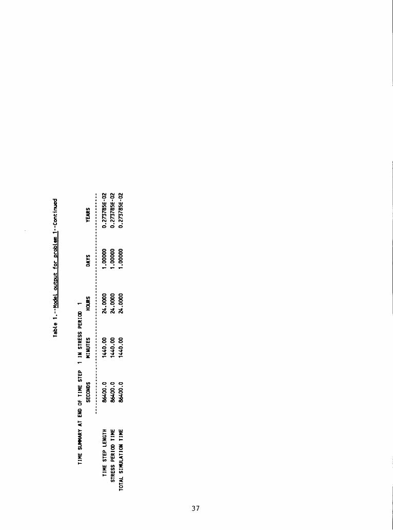
Tabl
e 1.--Model
output f
or p
robl
em I
Con
tinu
ed
TIME
SUMMARY
AT EN
D OF
TIME STEP
1 IN STRESS P
ERIOD
1SE
COND
S MINUTES
HOURS
TIME
STEP L
ENGTH
STRESS P
ERIOD
TIME
TOTA
L SI
MULA
TION
TIME
86400.0
86400.0
8640
0.0
1440
.00
1440
.00
1440
.00
24.0
000
24.0
000
24.0000
DAYS
YEAR
S
1.00
000
1.00
000
1.00
000
0.273785E-02
0.273785E-02
0.273785E-02
OJ
wet. It is also possible to use a larger positive wetting threshold to
prevent these cells from incorrectly becoming wet.
Validation of Results
There is no known analytical solution for this problem. Several
simulations using the BCFl Package were made to show that the BCF2 results
are valid. To do these, initial heads were set so that all cells were
active, preventing the need to wet cells. In steady-state simulations,
problems occurred because of the drying of too many cells. Therefore, a
transient simulation was used to avoid the likelihood for cells to dry
unnecessarily. With initial heads of 140 feet and all cells active, the
natural and stressed conditions could be simulated in two successive stress
periods in much the same way as done in the BCF2 simulation. Each stress
period lasted 90,000 days, had 20 time steps, and a time step multiplier of
1.1. The specific yield for layer 1 was 0.2. By the end of the last time
step, heads were essentially at steady state.
There were differences between the results from the BCF2 simulation and
the transient BCFl simulation. Cells in column 10 of layer 1 at the end of
stress period 2 were dry in the BCF2 simulation and wet in the BCFl
simulation. The result is that heads in the BCFl simulation are as much as
1 foot lower than heads in the BCF2 simulation. Analysis shows that the
differences between the BCFl and BCF2 simulations are not caused by errors
in the BCF2 code. In fact, a transient BCF2 simulation was made that
reproduced the BCFl results exactly. Rather, the differences are caused by
the non-unique solutions that can result from the method of solving the
nonlinear equations as described previously. The cells in column 10 went
dry in the BCF2 simulation because of overshoot in the iterative convergence
process. Once they went dry, heads did not go high enough to cause these
cells to rewet. In the steady-state BCF2 simulation, the head in column 10
of layer 2 was about 0.8 foot above the bottom of layer 1; the wetting
threshold was 2 feet. The effects of flow from storage minimized the
overshoot in the BCFl transient simulation, allowing the cells in column 10
to stay wet. These simulations show that, with the specified wetting
38
criteria, a range of solutions is possible, depending on numerical
subtleties of the solution process. The range of uncertainty can be
minimized by using a smaller wetting threshold, but this is at the risk of
causing instability in the solution process.
Problem 2 -- Simulation of a Water-Table Mound in Resulting
from Local Recharge
Localized recharge to a water-table aquifer results in formation of a
ground-water mound. For example, a ground-water mound may form in response
to recharge from infiltration ponds commonly used to artificially replenish
aquifers or to remove contamination by filtration through a soil column. If
the aquifer has low vertical hydraulic conductivity or contains interspersed
zones of low hydraulic conductivity, it may be necessary to simulate the
aquifer using multiple model layers in which the mound crosses more than one
layer. The BCF1 Package could not be used for such a simulation because
cells cannot change from no-flow to variable head, and the simulated mound
could not build up into previously dry layers. The following hypothetical
problem was posed to evaluate the capability of the BCF2 Package to simulate
mounding of the water table through multiple model layers.
Conceptual Model
The conceptual model consists of a rectangular, unconfined aquifer
overlain by a thick unsaturated zone (fig. 2). The horizontal hydraulic
conductivity is 5 feet per day and vertical hydraulic conductivity is 0.25
feet per day. A leaking pond recharges the aquifer, resulting in the
formation of a ground-water mound. The pond covers approximately 6 acres
and pond leakage is 12,500 cubic feet per day (65 gallons per minute). The
specific yield is 20 percent. The water table is flat prior to the creation
of the recharge pond. The flat water table is the result of a uniform
constant-head boundary that surrounds the aquifer.
39

1 70
a 60 cc
I 50mcc
40
30UJu.
-. 20 o
§LU
10
Infiltration pond Land surface ^^ ~~^L
Pond leakage {"
i
Ground-water mound /'
>
Water table ___--"'
Ratio of horizontal to vertical hydraulic conductivity
is 20 to 1
-- ^*
-1(
, ,
\
\V
V
\\ ^ - - - -. - ..
L J\ r< r
1
1
1
1
1
12
3
4
5
6
7
8
g0
12
3
4
1
sK;
vE
? :
I
CROSS-SECTIONCells with assigned constant heads of 25 feet
Column 1234
&,',','.'.'.',
/: : : : : :« :
/=*
liHilii^ i:¥:S5:§:S:
125ft
125ft
125ft
125ft
MODEL GRID CONFIGURATION
20 30 40
Figure 2.-Hydrogeology, model grid, and model boundary conditions for problem 2.
40
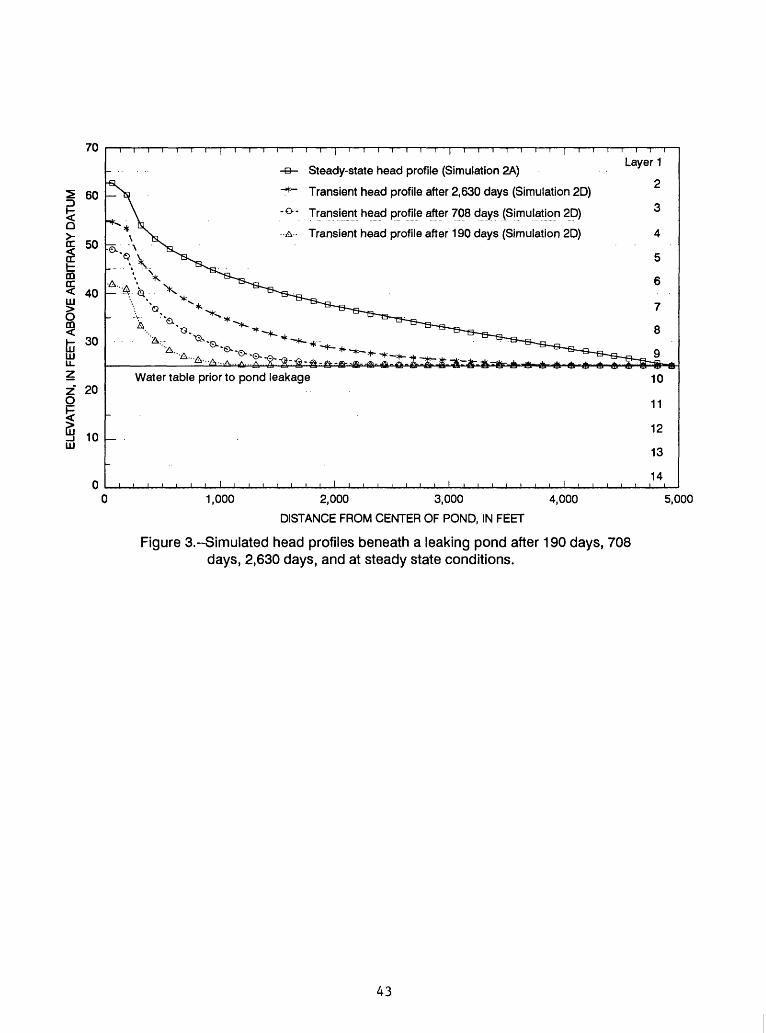
Ife ICD
HI
ItuHI
ZoIHI
70
60
50
40
30
20
10
-a- Steady-state head profile (Simulation 2A)
~*~ Transient head profile after 2,630 days (Simulation 2D)
-°-- Transient head profile after 708 days (Simulation 2D)
A Transient head profile after 190 days (Simulation 2D)
Water table prior to pond leakage
i i
Layer 1
2
3
4
5
6
7
8
9 *10
11
12
13
14
1,000 2,000 3,000
DISTANCE FROM CENTER OF POND, IN FEET
4,000
Figure 3.-Simulated head profiles beneath a leaking pond after 190 days, 708 days, 2,630 days, and at steady state conditions.
5,000
43

steepness of the head gradient and the grid discretization, the head
difference between adjacent horizontal cells is generally much larger than
the head difference between adjacent vertical cells along the mound. For
example, the cell at layer 4, row 3, column 4 is supposed to be dry even
though the head in the horizontally adjacent cell in column 3 is 1.4 feet
above the bottom of the layer. The vertical head difference between cells
in this part of the model is much less; the difference between the head at
the cell in layer 4, row 3, column 3 and the cell below is only 0.05 foot.
Thus, the neighboring cell to the right is repeatedly and incorrectly
converted to wet during the solution process if horizontal wetting is used
with a wetting threshold of 0.5 foot. The larger wetting threshold and
wetting-iteration interval used in Simulation 2B allow convergence to occur,
but only after many iterations. In this simulation, head in adjacent
vertical cells is the best indicator of when a dry cell should become wet.
Both simulations gave similar results with minor differences in which
cells were wet. For example, Simulation 2A has one wet cell in layer two
while Simulation 2B has three wet cells in layer 2. However there were 244
less wet cells for Simulation 2B. This is because the higher wetting
threshold of Simulation 2B prevented some cells from wetting that would have
wetted with a lower threshold. Head differences between the two solutions
generally were 0.05 foot or less with the exception of head at a few cells
near the areas where the two simulations differed in which cells were wet.
Head differences of about 0.1 foot were noted in these cells. The
volumetric budget error for both solutions was zero.
A SIP solution to the steady-state ground-water mounding problem,
Simulation 2C, was also obtained. In this simulation, cells were activated
by comparison only to head in underlying cells. Wetting and SIP solver
parameters were adjusted to minimize the required iterations (table 2). The
wetting iteration interval was experimentally set at 11 iterations. The
wetting threshold and wetting factor were set at 0.5 foot and 1.0, respect
ively. The solution met the head-change criterion for closure in 827 itera
tions, resulting in a budget error of 0.04 percent. This simulation took
much more computer time than either PCG2 simulation. There were 43 less wet
cells than in Simulation 2A. Heads matched Simulation 2A within 0.05 foot.
44
Modeling Approach
Because of the symmetry, heads are identical in each quadrant of the
aquifer, and there is no flow between quadrants; therefore, only one quarter
of the system needs to be simulated. The problem is simulated using a grid
of 40 rows, 40 columns, and 14 layers (fig. 2). A uniform horizontal grid
spacing of 125 feet is used, and each layer is 5 feet thick. The pond is in
the upper left corner of the grid. The boundaries along row 1 and column 1
are no-flow as a result of the symmetry. A constant-head boundary of 25
feet is specified along row 40 and column 40 for layers 10-14; a no-flow
boundary is assigned along row 40 and column 40 for layers 1-9. Without the
recharge from the pond, layers 1-9 are dry, and the head in all the cells of
layers 10-14 is 25 feet.
Recharge from the pond is applied to the horizontal area encompassed by
rows 1 through 2 and columns 1 through 2. Recharge option 3 (McDonald and
Harbaugh, 1988, p. 7-2) is used so that recharge will penetrate through
inactive cells down to the water table. The recharge rate of 0.05 foot per
day simulates leakage of 3,125 cubic feet per day (16.2 gallons per minute)
through one quarter of the pond bottom, a simulated area of 62,500 square
feet.
Simulation Results
Steady-state and transient simulations were made to demonstrate the
capability of the BCF2 Package to simulate the formation of the mound.
Solution of the flow equations was attempted using both the PCG2 solver and
the SIP solver. Also, several combinations of the BCF2 parameters that
affect stability of the wetting process were used. Wetting and solver
parameters are shown in table 2 for comparison.
41

Table 2. - - Wetting and solver input data for Problem 2 simulations
Parameter
WETDRY (feet)
Equation used for calculating
head at a cell that is wetted
Wetting factor (WETFCT)
Wetting iteration interval (IWETIT)
Solver
Head- change closure criterion (feet)
PCG residual closure
criterion (cubic feet)
PCG maximum inner iterations
SIP WSEED
Simulation
2A
-0.5
3a
0.5
1
PCG2
0.001
1000.
20
N/A
Simulation
2B
1.5
3a
0.5
2
PCG2
0.001
1000.
20
N/A
Simulation
2C
-0.5
3b
1.0
11
SIP
0.00001
N/A
N/A
0.002
For the steady-state problem, the least computational time was required
when using the PCG2 solver. Reasonable solutions to the ground-water mound
ing problem were obtained in two steady-state PCG2 simulations. In the
first simulation, Simulation 2A, dry cells were converted to wet by compari
son of the wetting threshold to head only in underlying cells, which is
indicated by a negative WETDRY parameter. The wetting-iteration interval
was 1 and the WETDRY parameter was -0.5 foot, which means that the wetting
threshold is 10 percent of the thickness of a cell. Solution was achieved
in 11 outer iterations and 179 total iterations. Figure 3 shows results
from Simulation 2A.
In the second PCG2 simulation, Simulation 2B, wetting of cells was
based on comparison to heads both in horizontally adjacent and underlying
cells (WETDRY parameter is positive). A wetting-iteration interval of 2 and
a WETDRY parameter of 1.5 feet were used in order to prevent continued
oscillation between wet and dry for some cells. Solution was obtained in 23
outer iterations and 420 total iterations.
The use of horizontal wetting resulted in additional iterations for the
second simulation and the need to change wetting parameters. Due to the
42
A steady-state SIP solution in which cells were activated by comparison
of the wetting threshold to heads in horizontally adjacent and underlying
cells could not be obtained despite experimental variation of WSEED and the
wetting iteration interval. Chaotic wetting and drying of cells caused the
simulation to terminate with divide-by-zero errors due to isolated groups of
active cells.
The formation of the ground-water mound was simulated over time with a
transient simulation, Simulation 2D. The transient simulation was run for
one stress period with a length of 500,000 days. The stress period was
divided into 50 time steps with a time-step multiplier of 1.3. The first
time step was 0.3 days, and the last time step was 115,000 days. Transient
simulations used a specific yield of 20 percent and a confined storage
coefficient of 0.001. The PCG2 solver was used and cells were activated by
comparison of the wetting threshold to heads in underlying cells. The head-
change criterion for closure was 0.001 foot and the residual-change
criterion was 10,000 cubic feet, the wetting threshold was 0.5 foot, the
wetting factor was 0.5, and the wetting-iteration interval was 1. Figure 3
shows simulated water-table heads along row 1 at several times during the
transient simulation.
Steady-state conditions were reached at the end of the transient
simulation as indicated by storage flow terms being zero. Simulation 2D had
43 less wet cells at the end than did Simulation 2A. Heads at the end of
Simulation 2D were within 0.02 foot of the heads in Simulation 2A. The
volumetric budget error at the end of the stress period was 0.02 percent.
Validation of Results
The ground-water mounding problem is nonlinear, precluding comparison
to an analytical solution. The steady-state solution from Simulation 2A was
compared to two BCF1 simulations to show that the solution was reasonable.
The mounding problem theoretically can be simulated by the BCF1 Package
in steady state if initial heads are above the final heads. That is, BCF1
45
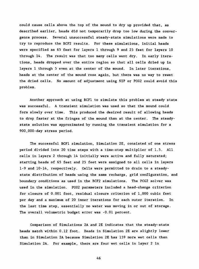
could cause cells above the top of the mound to dry up provided that, as
described earlier, heads did not temporarily drop too low during the conver
gence process. Several unsuccessful steady-state simulations were made to
try to reproduce the BCF2 results. For these simulations, initial heads
were specified as 65 feet for layers 1 through 9 and 25 feet for layers 10
through 14. The result was that too many cells went dry. In early itera
tions, heads dropped over the entire region so that all cells dried up in
layers 1 through 5 even at the center of the mound. In later iterations,
heads at the center of the mound rose again, but there was no way to rewet
the dried cells. No amount of adjustment using SIP or PCG2 could avoid this
problem.
Another approach at using BCF1 to simulate this problem at steady state
was successful. A transient simulation was used so that the mound could
form slowly over time. This produced the desired result of allowing heads
to drop faster at the fringes of the mound than at the center. The steady-
state solution was approximated by running the transient simulation for a
900,000-day stress period.
The successful BCF1 simulation, Simulation 2E, consisted of one stress
period divided into 20 time steps with a time-step multiplier of 1.5. All
cells in layers 2 through 14 initially were active and fully saturated;
starting heads of 65 feet and 25 feet were assigned to all cells in layers
1-9 and 10-14, respectively. Cells were permitted to drain to a steady-
state distribution of heads using the same recharge, grid configuration, and
boundary conditions as used in the BCF2 simulations. The PCG2 solver was
used in the simulation. PCG2 parameters included a head-change criterion
for closure of 0.001 foot, residual closure criterion of 1,000 cubic feet
per day and a maximum of 20 inner iterations for each outer iteration. In
the last time step, essentially no water was moving in or out of storage.
The overall volumetric budget error was -0.01 percent.
Comparison of Simulations 2A and 2E indicates that the steady-state
heads match within 0.12 foot. Heads in Simulation 2E are slightly lower
than in Simulation 2A because Simulation 2E has 159 more wet cells than
Simulation 2A. For example, there are four wet cells in layer 2 in
46
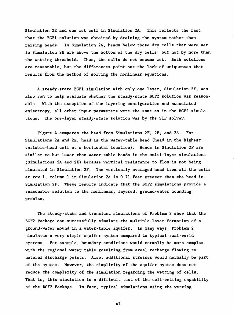
Simulation 2E and one wet cell in Simulation 2A. This reflects the fact
that the BCF1 solution was obtained by draining the system rather than
raising heads. In Simulation 2A, heads below those dry cells that were wet
in Simulation 2E are above the bottom of the dry cells, but not by more than
the wetting threshold. Thus, the cells do not become wet. Both solutions
are reasonable, but the differences point out the lack of uniqueness that
results from the method of solving the nonlinear equations.
A steady-state BCF1 simulation with only one layer, Simulation 2F, was
also run to help evaluate whether the steady-state BCF2 solution was reason
able. With the exception of the layering configuration and associated
anisotropy, all other input parameters were the same as in the BCF2 simula
tions. The one-layer steady-state solution was by the SIP solver.
Figure 4 compares the head from Simulations 2F, 2E, and 2A. For
Simulations 2A and 2E, head is the water-table head (head in the highest
variable-head cell at a horizontal location). Heads in Simulation 2F are
similar to but lower than water-table heads in the multi-layer simulations
(Simulations 2A and 2E) because vertical resistance to flow is not being
simulated in Simulation 2F. The vertically averaged head from all the cells
at row 1, column 1 in Simulation 2A is 0.71 feet greater than the head in
Simulation 2F. These results indicate that the BCF2 simulations provide a
reasonable solution to the nonlinear, layered, ground-water mounding
problem.
The steady-state and transient simulations of Problem 2 show that the
BCF2 Package can successfully simulate the multiple-layer formation of a
ground-water mound in a water-table aquifer. In many ways, Problem 2
simulates a very simple aquifer system compared to typical real-world
systems. For example, boundary conditions would normally be more complex
with the regional water table resulting from areal recharge flowing to
natural discharge points. Also, additional stresses would normally be part
of the system. However, the simplicity of the aquifer system does not
reduce the complexity of the simulation regarding the wetting of cells.
That is, this simulation is a difficult test of the cell-wetting capability
of the BCF2 Package. In fact, typical simulations using the wetting
47
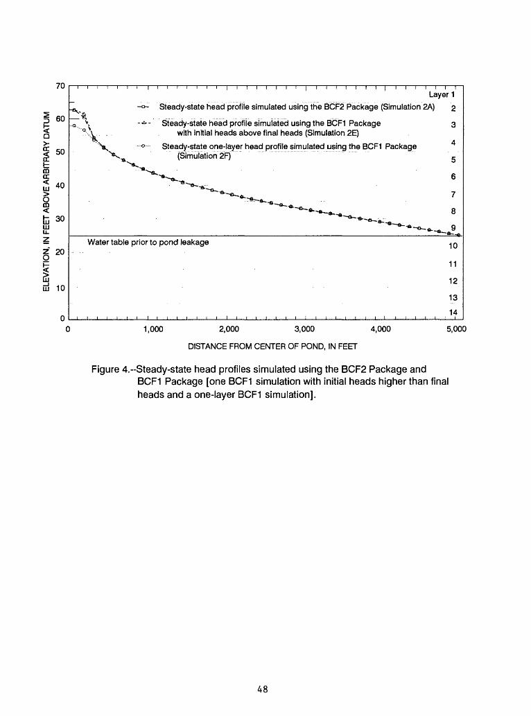
70 I I I I I I I I I I I 1 I I 1 1 1 I I I I
Layer 1
m DC <UJ
8m
60
50
«
*v.-, Steady-state head profile simulated using the BCF2 Package (Simulation 2A)
tD 30UJ
§ 20IuJ 10
Steady-state head profile simulated using the BCF1 Package with initial heads above final heads (Simulation 2E)
Steady-state one-layer head profile simulated using the BCF1 Package
Water table prior to pond leakage 10
11
12
13
14
1,000 2,000 3,000 4,000
DISTANCE FROM CENTER OF POND, IN FEET
5,000
Figure 4.-Steady-state head profiles simulated using the BCF2 Package andBCF1 Package [one BCF1 simulation with initial heads higher than final heads and a one-layer BCF1 simulation].
48
capability probably will not involve a water table crossing so many model
layers. For many purposes, this system could be simulated realistically
with less layers. The large number of layers was used in order to test the
BCF2 Package. With the water table crossing eight layers, there is a high
possibility of repeated wetting and drying of cells. Yet stable solutions
were obtained after moderate effort was used in selecting the various
parameters that affect solution stability.
Problem 3 -- Simulation of a Perched Water Table
Contrasts in vertical hydraulic conductivity within the unsaturated
zone can provide a mechanism for the formation of perched ground-water
tables. The formation of these bodies in a previously unsaturated zone is
difficult to simulate with the BCF1 Package because cells cannot change from
no-flow to variable-head conditions. A problem was posed to evaluate the
capability of the BCF2 Package to simulate formation of a perched water
table. This problem has practical application in the simulation of recharge
going to a deeper aquifer system.
Conceptual Model
The conceptual model is rectangular and consists of three geohydrologic
units. The upper and lower units have higher hydraulic conductivities than
the middle unit (fig. 5). There is a regional water table in which the head
is below the bottom of unit 2. Natural recharge occurs over the entire area
at a rate of 0.001 foot per day. This recharge can percolate through the
two upper units without the formation of a water table above unit 2 because
the vertical hydraulic conductivity of this middle unit is 0.002 foot per
day.
Recharge at a rate of 0.01 foot per day from a pond covering 6 acres
causes a perched ground-water body to form in the top two units. The total
pond leakage is about 2,360 cubic feet per day (12 gallons per minute). The
perched water table spreads out over an area much larger than the area
49
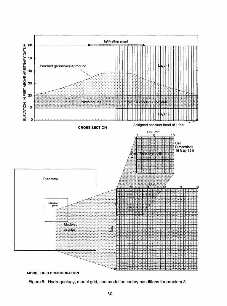
Q
OC < OC
2OC< 1118CD <
fc 111
60
50
40
30
20
10
Infiltration pond
Perched ground-water mound
CROSS SECTIONAssigned constant head of 1 foot
CellDimensions 16ft by 16ft
MODEL GRID CONFIGURATION
Figure 5.--Hydrogeology, model grid, and model boundary conditions for problem 3
50
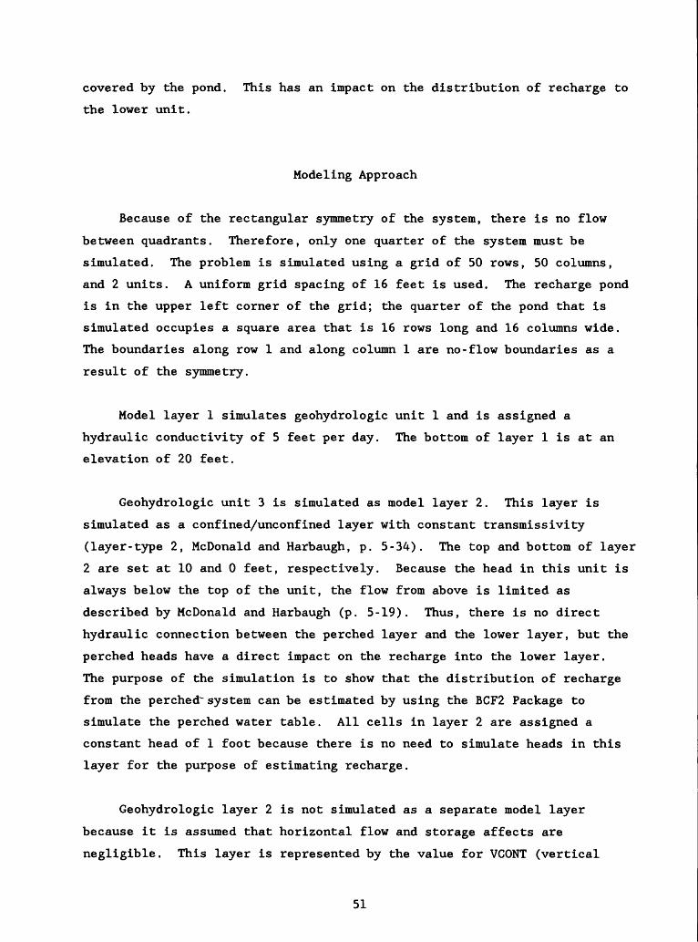
covered by the pond. This has an impact on the distribution of recharge to
the lower unit.
Modeling Approach
Because of the rectangular symmetry of the system, there is no flow
between quadrants. Therefore, only one quarter of the system must be
simulated. The problem is simulated using a grid of 50 rows, 50 columns,
and 2 units. A uniform grid spacing of 16 feet is used. The recharge pond
is in the upper left corner of the grid; the quarter of the pond that is
simulated occupies a square area that is 16 rows long and 16 columns wide.
The boundaries along row 1 and along column 1 are no-flow boundaries as a
result of the symmetry.
Model layer 1 simulates geohydrologic unit 1 and is assigned a
hydraulic conductivity of 5 feet per day. The bottom of layer 1 is at an
elevation of 20 feet.
Geohydrologic unit 3 is simulated as model layer 2. This layer is
simulated as a confined/unconfined layer with constant transmissivity
(layer-type 2, McDonald and Harbaugh, p. 5-34). The top and bottom of layer
2 are set at 10 and 0 feet, respectively. Because the head in this unit is
always below the top of the unit, the flow from above is limited as
described by McDonald and Harbaugh (p. 5-19). Thus, there is no direct
hydraulic connection between the perched layer and the lower layer, but the
perched heads have a direct impact on the recharge into the lower layer.
The purpose of the simulation is to show that the distribution of recharge
from the perched*system can be estimated by using the BCF2 Package to
simulate the perched water table. All cells in layer 2 are assigned a
constant head of 1 foot because there is no need to simulate heads in this
layer for the purpose of estimating recharge.
Geohydrologic layer 2 is not simulated as a separate model layer
because it is assumed that horizontal flow and storage affects are
negligible. This layer is represented by the value for VCONT (vertical
51
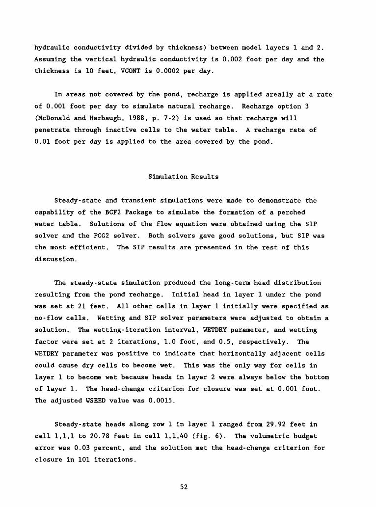
hydraulic conductivity divided by thickness) between model layers 1 and 2.
Assuming the vertical hydraulic conductivity is 0.002 foot per day and the
thickness is 10 feet, VCONT is 0.0002 per day.
In areas not covered by the pond, recharge is applied areally at a rate
of 0.001 foot per day to simulate natural recharge. Recharge option 3
(McDonald and Harbaugh, 1988, p. 7-2) is used so that recharge will
penetrate through inactive cells to the water table. A recharge rate of
0.01 foot per day is applied to the area covered by the pond.
Simulation Results
Steady-state and transient simulations were made to demonstrate the
capability of the BCF2 Package to simulate the formation of a perched
water table. Solutions of the flow equation were obtained using the SIP
solver and the PCG2 solver. Both solvers gave good solutions, but SIP was
the most efficient. The SIP results are presented in the rest of this
discussion.
The steady-state simulation produced the long-term head distribution
resulting from the pond recharge. Initial head in layer 1 under the pond
was set at 21 feet. All other cells in layer 1 initially were specified as
no-flow cells. Wetting and SIP solver parameters were adjusted to obtain a
solution. The wetting-iteration interval, WETDRY parameter, and wetting
factor were set at 2 iterations, 1.0 foot, and 0.5, respectively. The
WETDRY parameter was positive to indicate that horizontally adjacent cells
could cause dry cells to become wet. This was the only way for cells in
layer 1 to become wet because heads in layer 2 were always below the bottom
of layer 1. The head-change criterion for closure was set at 0.001 foot.
The adjusted WSEED value was 0.0015.
Steady-state heads along row 1 in layer 1 ranged from 29.92 feet in
cell 1,1,1 to 20.78 feet in cell 1,1,40 (fig. 6). The volumetric budget
error was 0.03 percent, and the solution met the head-change criterion for
closure in 101 iterations.
52
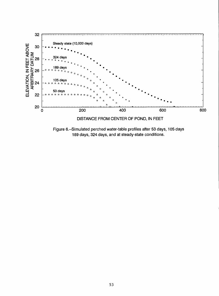
u>
ELE
VA
TIO
N,
IN F
EE
T A
BO
VE
A
RB
ITR
AR
Y D
AT
UM
_J.
00
CO Q.
j/> CO U
Q.
CO
*< j/> Q.
CD £ CD Q.
*< CO 1 o O D
Q.
o'
D
-n
ca" c CD O)
"i CO 3'
c
w CD
Q.
D
CD O CD
Q.
CD -^ co O" CD D O ^ C/) It CD 01
CO Q.
CO 0 01
Q.
CO C/)
r
o
2
roC
O
O
J
O> Z
O m
-n 33
O O
m z H
-U
m
o33
0
O Tl
TJ
O O Z Tl m H
§ 00 o o
0
K>
fO
IO
IO
CO
D
K)
4^
O)
CO
O
1 1
' 1
' 1
' 1
' 1
'[
D
>
O
*
; D
>
o
*
o t>
o
*
S-*
-*
CO
CO
c>
o °o
o
*ro
"/
J?
0)
Q.
Q.
* Q
. Q
.
D*"
>
^
T^
**^
B"*
^
D t>
o *
"2
. STD
>
O
»
ra
D
>
O
*
-* O
D
>
O
*
-
o >
o
*
O oD
>
0
*
_
D
>
O
*
0)
D
>
O
»
0)
D
>
O
*
D
>
O
*
t>
O
*
t>
O
*
t>
O
*
O
*
0
*
o »
*
*
*
*
mm
mm
fm
m
1,1,1,1,1,
CO rv3 _ - - _ -_ - - i _ ~ : -_ -_ -_ - ~ - - : - - - ~ ~ - _ ~ 5 ; I - - - ;
The formation of the perched water table was simulated over time in a
transient simulation. The transient simulation was run for one stress
period with a length of 10,000 days. The stress period was divided into 60
time steps with a time-step multiplier of 1.1. The specific yield was 20
percent. The wetting-iteration interval and wetting factor were experi
mentally set at 1 iteration and 0.1, respectively. The WETDRY parameter was
1.3 feet in the square area defined by rows 1-18 and columns 1-18, and
everywhere else WETDRY was 1 foot. Initially, WETDRY was set to 1 foot
everywhere, but this resulted in instability in early time. This may have
been caused by the steeper head gradients that occur in early time as the
mound began to form. Also, as described earlier, small time steps can
contribute to instability due to the resulting large rates of flow from
storage. The adjusted WSEED value was 0.0001. Initial heads of 20.01 feet
were set at the cells below the pond. All other cells in layer 1 initially
were no flow.
Transient heads along row 1 of layer 1 are shown in figure 6 at times
of 53 days, 105 days, 189 days, and 324 days. The volumetric budget error
was zero. After 10,000 days, heads essentially were at steady state because
flow into storage was zero. Heads at the end of the transient simulation
matched the heads from the steady-state simulation within 0.02 foot.
Validation of Results
The perched water-table problem is nonlinear, precluding comparison to
an analytical solution. Comparison of the steady-state and transient
solutions indicated that the BCF2 simulations reasonably solved the problem.
The steady-state BCF2 solution also was compared to a transient BCF1
simulation to determine whether the solution was reasonable.
The BCF1 transient solution to the perched water-table problem was
simulated by permitting cells to drain to a steady-state configuration. All
cells in layer 1 initially were active with a starting head of 30 feet. SIP
solver parameters were the same as those used in the BCF2 solutions. The
simulation was run for 10,000 days, using 100 time steps and a time-step
54
multiplier of 1.1. The volumetric budget error at the end of the 10,000
days was zero.
The steady-state heads were very similar in the two simulations, but
the BCF1 steady-state heads were as much as 0.6 foot lower than the BCF2
steady-state heads near the edges of the perched water table. In the BCF1
simulation, the heads were draining from high initial values while in the
the BCF2 simulation, heads rose from low initial values. Thus, some cells
remained wet in the BCF1 simulation that did not become wet in the BCF2
simulation because the wetting threshold was not exceeded. The larger
extent of the water table in the BCF1 simulation caused the slightly lower
heads.
MODULE DOCUMENTATION
The design of the BCF2 Package closely follows the design of the BCF1
Package. Several of the BCF2 modules are identical to BCF1 modules, and the
replaced modules are very similar in function and structure to the previous
modules. There is one new module, BCF2AD. The unchanged modules have not
been given new names. That is, the unchanged modules retain the revision
level "1" in their names. Accordingly, the BCF2 Package consists of the
following modules: BCF2AL, BCF2RP, BCF2AD, BCF2FM, BCF1BD, SBCF2N, SBCF2H,
SBCF1C, SBCF1B, SBCF1F. This report contains documentation for all of the
new modules. Refer to McDonald and Harbaugh (1988, Ch. 5) for documentation
of unchanged modules.
In the model program, each package is assigned a file unit on which to
read input data. The file unit for the BCF2 Package is assumed to be the
same input unit that is used by the BCF1 Package, which is the first element
in the IUNIT array [IUNIT(1)]. Because the BCF2 Package contains all of the
functionality of the BCF1 Package, there is no need to retain the BCF1
Package as a separate package in the model program.
55
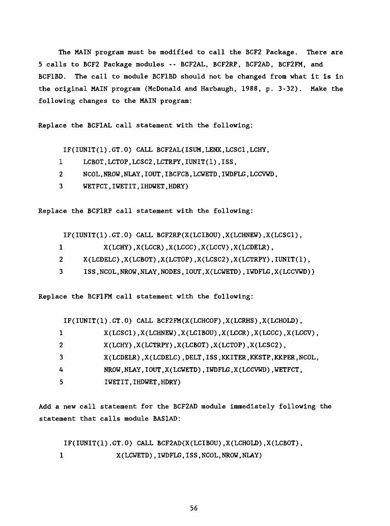
The MAIN program must be modified to call the BCF2 Package. There are
5 calls to BCF2 Package modules -- BCF2AL, BCF2RP, BCF2AD, BCF2FM, and
BCF1BD. The call to module BCF1BD should not be changed from what it is in
the original MAIN program (McDonald and Harbaugh, 1988, p. 3-32). Make the
following changes to the MAIN program:
Replace the BCFlAL call statement with the following:
IF(IUNIT(1).GT.O) CALL BCF2AL(ISUM,LENX,LCSC1,LCHY,
1 LCBOT,LCTOP,LCSC2,LCTRPY,IUNIT(1),ISS,
2 NCOL,NROW,NLAY,IOUT,IBCFCB,LCWETD,IWDFLG,LCCVWD,
3 WETFCT,IWETIT,IHDWET,HDRY)
Replace the BCF1RP call statement with the following:
IF(IUNIT(1).GT.O) CALL BCF2RP(X(LCIBOU),X(LCHNEW),X(LCSC1),
1 X(LCHY),X(LCCR),X(LCCC),X(LCCV),X(LCDELR),
2 X(LCDELC),X(LCBOT),X(LCTOP),X(LCSC2),X(LCTRPY),IUNIT(1),
3 ISS,NCOL,NROW,NLAY,NODES,IOUT,X(LCWETD),IWDFLG,X(LCCVWD))
Replace the BCF1FM call statement with the following:
IF(IUNIT(1).GT.O) CALL BCF2FM(X(LCHCOF),X(LCRHS),X(LCHOLD),
1 X(LCSCl),X(LCHNEW),X(LCIBOU),X(LCCR),X(LCCC),X(LCCV),
2 X(LCHY),X(LCTRPY),X(LCBOT),X(LCTOP),X(LCSC2),
3 X(LCDELR),X(LCDELC),DELT,ISS,KKITER,KKSTP,KKPER,NCOL,
4 NROW,NLAY,IOUT,X(LCWETD),IWDFLG,X(LCCVWD),WETFCT,
5 IWETIT,IHDWET,HDRY)
Add a new call statement for the BCF2AD module immediately following the
statement that calls module BAS1AD:
IF(IUNIT(1).GT.O) CALL BCF2AD(X(LCIBOU),X(LCHOLD),X(LCBOT),
1 X(LCWETD),IWDFLG,ISS,NCOL,NROW,NLAY)
56
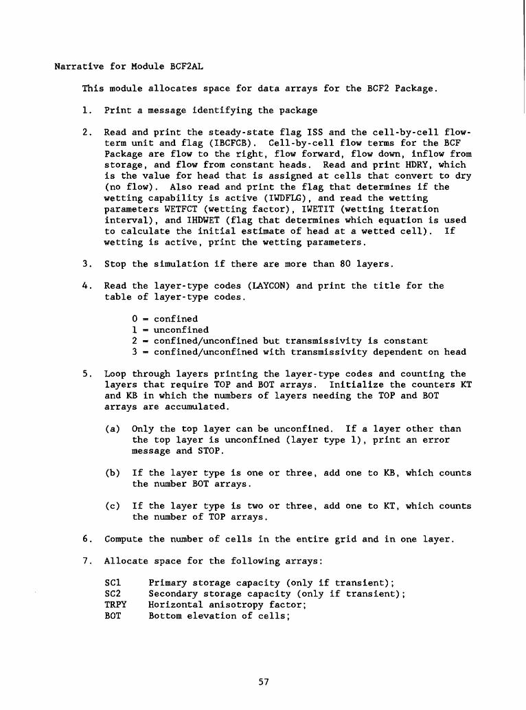
Narrative for Module BCF2AL
This module allocates space for data arrays for the BCF2 Package.
1. Print a message identifying the package
2. Read and print the steady-state flag ISS and the cell-by-cell flow- term unit and flag (IBCFCB). Cell-by-cell flow terms for the BCF Package are flow to the right, flow forward, flow down, inflow from storage, and flow from constant heads. Read and print HDRY, which is the value for head that is assigned at cells that convert to dry (no flow). Also read and print the flag that determines if the wetting capability is active (IWDFLG), and read the wetting parameters WETFCT (wetting factor), IWETIT (wetting iteration interval), and IHDWET (flag that determines which equation is used to calculate the initial estimate of head at a wetted cell). If wetting is active, print the wetting parameters.
3. Stop the simulation if there are more than 80 layers.
4. Read the layer-type codes (LAYCON) and print the title for the table of layer-type codes.
0 - confined1 - unconfined2 - confined/unconfined but transmissivity is constant3 - confined/unconfined with transmissivity dependent on head
5. Loop through layers printing the layer-type codes and counting the layers that require TOP and BOT arrays. Initialize the counters KT and KB in which the numbers of layers needing the TOP and BOT arrays are accumulated.
(a) Only the top layer can be unconfined. If a layer other than the top layer is unconfined (layer type 1), print an error message and STOP.
(b) If the layer type is one or three, add one to KB, which counts the number BOT arrays.
(c) If the layer type is two or three, add one to KT, which counts the number of TOP arrays.
6. Compute the number of cells in the entire grid and in one layer.
7. Allocate space for the following arrays:
SCI Primary storage capacity (only if transient);SC2 Secondary storage capacity (only if transient);TRPY Horizontal anisotropy factor;BOT Bottom elevation of cells;
57
HY Hydraulic conductivity; TOP Top elevation of cells;WETD Wetting threshold (only when wetting is active); and CVWD Initial values of vertical conductance (only when wetting
is active).
8. Print the amount of space used by the BCF Package.
9. RETURN.
58
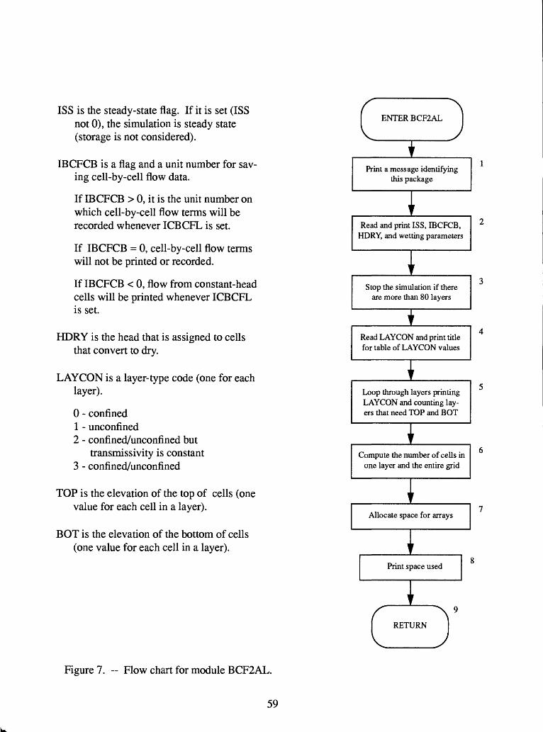
ISS is the steady-state flag. If it is set (ISS not 0), the simulation is steady state (storage is not considered).
IBCFCB is a flag and a unit number for sav ing cell-by-cell flow data.
If IBCFCB > 0, it is the unit number on which cell-by-cell flow terms will be recorded whenever ICBCFL is set.
If IBCFCB = 0, cell-by-cell flow terms will not be printed or recorded.
If IBCFCB < 0, flow from constant-head cells will be printed whenever ICBCFL is set.
HDRY is the head that is assigned to cells that convert to dry.
LAYCON is a layer-type code (one for each layer).
0 - confined1 - unconfined2 - confined/unconfined but
transmissivity is constant3 - confined/unconfined
TOP is the elevation of the top of cells (one value for each cell in a layer).
BOT is the elevation of the bottom of cells (one value for each cell in a layer).
ENTER BCF2AL
iPrint a message identifying
this package
Read and print ISS, IBCFCB, HDRY, and wetting parameters
Stop the simulation if there are more than 80 layers
Read LAYCON and print title for table of LAYCON values
ILoop through layers printing LAYCON and counting lay ers that need TOP and BOT
ICompute the number of cells in
one layer and the entire grid
iAllocate space for arrays
Print space used
Figure 7. ~ Flow chart for module BCF2AL.
RETURN
59

SUBROUTINE BCF2AL(ISUM,LENX,LCSC1,LCHY,LCBOT,LCTOP,LCSC2,LCTRPY,1 IN,ISS,NCOL,NROW,NLAY,IOUT,IBCFCB,LCWETD,IWDFLG,LCCVWD,2 WETFCT,IWETIT,IHDWET,HDRY)
C C--.--VERSION 1435 14MAY1991 BCF2AL
C ALLOCATE ARRAY STORAGE FOR BLOCK-CENTERED FLOW PACKAGE, VERSION 2
CC SPECIFICATIONS:C ..................................................................
COMMON /FLWCOM/LAYCON(80) C ..................................................................Cd------IDENTIFY PACKAGE
WRITE(IOUT,1)IN1 FORMAT(1HO,'BCF2 -- BLOCK-CENTERED FLOW PACKAGE, VERSION 2',1', 7/1/91',' INPUT READ FROM UNIT',13)
C C2------READ AND PRINT ISS (STEADY-STATE FLAG), IBCFCB (FLAG FORC2------PRINTING OR UNIT* FOR RECORDING CELL-BY-CELL FLOW TERMS),C2------HDRY (HEAD AT CELLS THAT CONVERT TO DRY), AND WETTING PARAMETERS
READ(IN,2) ISS,IBCFCB,HDRY,IWDFLG,WETFCT,IWETIT,IHDWET2 FORMAT(2I10,F10.0,110,F10.0,2110)
IF(ISS.EQ.O) WRITE(IOUT,3)3 FORMAT(IX,'TRANSIENT SIMULATION')
IF(ISS.NE.O) WRITE(IOUT,4)4 FORMAT(IX,'STEADY-STATE SIMULATION')
IF(IBCFCB.GT.O) WRITE(IOUT,9) IBCFCB9 FORMAT(IX,'CELL-BY-CELL FLOWS WILL BE RECORDED ON UNIT',13)
IF(IBCFCB.LT.O) WRITE(IOUT,88)88 FORMAT(IX,'CONSTANT HEAD CELL-BY-CELL FLOWS WILL BE PRINTED')
WRITE(IOUT,89) HDRY89 FORMAT(IX,'HEAD AT CELLS THAT CONVERT TO DRY-',G13.5)
IF(IWDFLG.NE.O) GO TO 35WRITE(IOUT,31)
31 FORMAT(IX,'WETTING CAPABILITY IS NOT ACTIVE')GO TO 39
C35 WRITE(IOUT,36)36 FORMAT(IX,'WETTING CAPABILITY IS ACTIVE')
IF(IWETIT.LE.O) IWETIT-1 WRITE(IOUT,37)WETFCT,IWETIT
37 FORMAT(IX,'WETTING FACTOR-',F10.5,1 ' WETTING ITERATION INTERVAL-',14) WRITE(IOUT,38)IHDWET
38 FORMAT(IX,'FLAG THAT SPECIFIES THE EQUATION TO USE FOR HEAD AT WET1TED CELLS-',14)
C C3......STOP THE SIMULATION IF THERE ARE MORE THAN 80 LAYERS
39 IF(NLAY.LE.SO) GO TO 50WRITE(IOUT,11)
11 FORMAT(1HO,'YOU HAVE SPECIFIED MORE THAN 80 MODEL LAYERS'/1X, 1 'SPACE IS RESERVED FOR A MAXIMUM OF 80 LAYERS IN ARRAY LAYCON')
60
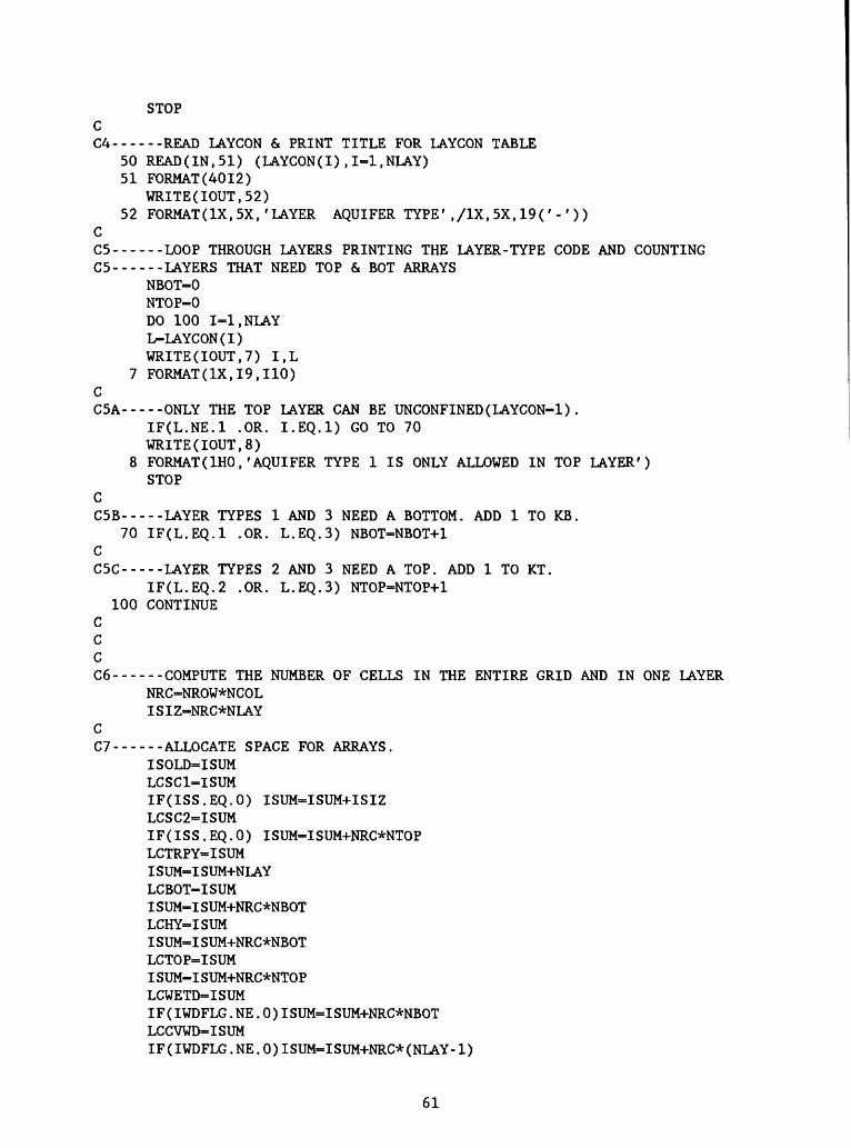
STOP C C4------READ LAYCON 6e PRINT TITLE FOR LAYCON TABLE
50 READ(IN,51) (LAYCON(I),I-1,NLAY)51 FORMAT(4012)
WRITE(IOUT,52)52 FORMAT(IX,5X/LAYER AQUIFER TYPE',/lX,5X,19('-'))
C C5------LOOP THROUGH LAYERS PRINTING THE LAYER-TYPE CODE AND COUNTINGC5------LAYERS THAT NEED TOP & EOT ARRAYS
NBOT=0NTOP=0DO 100 I=1,NLAYL-LAYCON(I)WRITE(IOUT,7) I,L
7 FORMAT(1X,I9,I10) CC5A-----ONLY THE TOP LAYER CAN BE UNCONFINED(LAYCON=1).
IF(L.NE.l .OR. I.EQ.l) GO TO 70 WRITE(IOUT,8)
8 FORMAT(IHO,'AQUIFER TYPE 1 IS ONLY ALLOWED IN TOP LAYER')STOP
C C5B-----LAYER TYPES 1 AND 3 NEED A BOTTOM. ADD 1 TO KB.
70 IF(L.EQ.l .OR. L.EQ.3) NBOT=NBOT+1 C CSC-----LAYER TYPES 2 AND 3 NEED A TOP. ADD 1 TO KT.
IF(L.EQ.2 .OR. L.EQ.3) NTOP=NTOP+1 100 CONTINUE
C C C C6------COMPUTE THE NUMBER OF CELLS IN THE ENTIRE GRID AND IN ONE LAYER
NRC=NROW*NCOLISIZ=NRC*NLAY
C C7------ALLOCATE SPACE FOR ARRAYS.
ISOLD-ISUMLCSC1=ISUMIF(ISS.EQ.O) ISUM=ISUM+ISIZLCSC2=ISUMIF(ISS.EQ.O) ISUM=ISUM+NRC*NTOPLCTRPY=ISUMISUM-ISUM+NLAYLCBOT=ISUMISUM=ISUM+NRC*NBOTLCHY-ISUMISUM=ISUM+NRC*NBOTLCTOP=ISUMISUM=ISUM+NRC*NTOPLCWETD=ISUMIF(IWDFLG.NE.0)ISUM=ISUM+NRC*NBOTLCCVWD=ISUMIF(IWDFLG.NE.0)ISUM=ISUM+NRC*(NLAY-1)
61
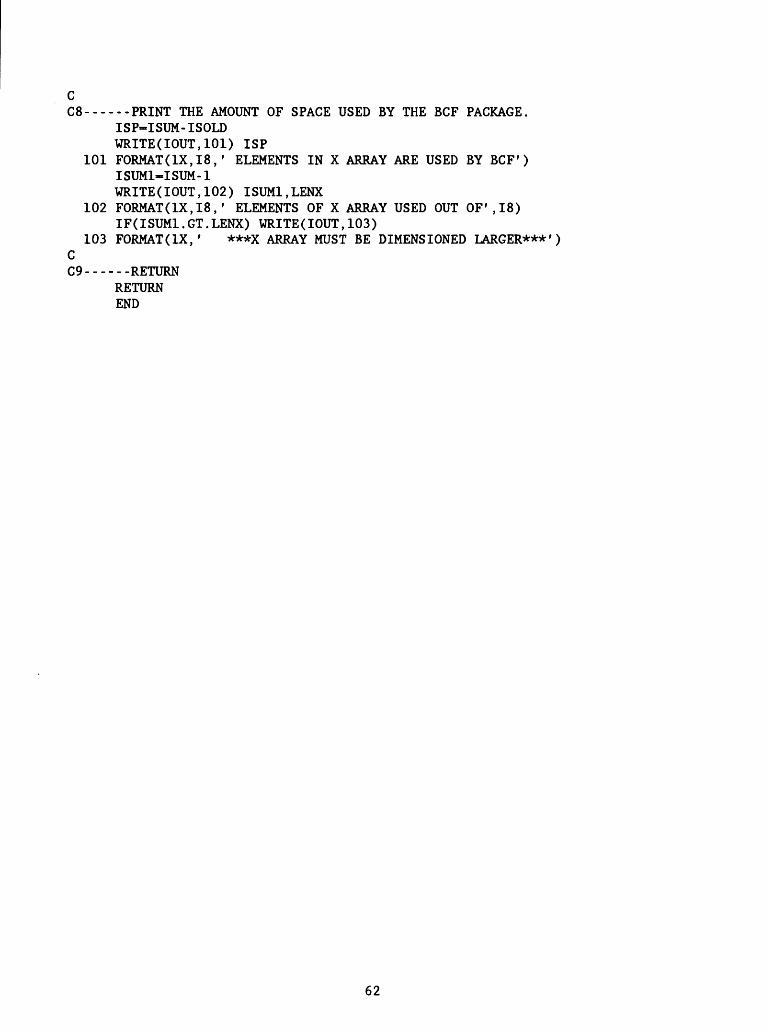
cC8------PRINT THE AMOUNT OF SPACE USED BY THE BCF PACKAGE.
ISP-ISUM-ISOLD WRITE(IOUT,101) ISP
101 FORMAT(IX,18,' ELEMENTS IN X ARRAY ARE USED BY BCF') ISUM1-ISUM-1 WRITE(IOUT,102) ISUM1.LENX
102 FORMAT(1X,I8,' ELEMENTS OF X ARRAY USED OUT OF',18) IF(ISUMl.GT.LENX) WRITE(IOUT,103)
103 FORMAT(IX,' ***X ARRAY MUST BE DIMENSIONED LARGER***') C C9------RETURN
RETURNEND
62
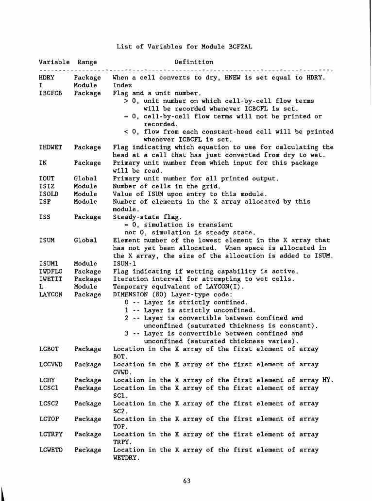
List of Variables for Module BCF2AL
Variable Range Definition
HDRY PackageI ModuleIBCFCB Package
IHDWET
IN
TOUT ISIZ ISOLD ISP
ISS
ISUM
LCBOT
LCCWD
LCHY LCSC1
LCSC2
LCTOP
LCTRPY
LCWETD
Package
Package
Global Module Module Module
Package
Global
ISUM1IWDFLG IWETIT LLAYCON
ModulePackage Package ModulePackage
Package
Package
Package Package
Package
Package
Package
Package
When a cell converts to dry, KNEW is set equal to HDRY.IndexFlag and a unit number.
> 0, unit number on which cell-by-cell flow terms will be recorded whenever ICBCFL is set.
= 0, cell-by-cell flow terms will not be printed or recorded.
< 0, flow from each constant-head cell will be printedwhenever ICBCFL is set.
Flag indicating which equation to use for calculating the head at a cell that has just converted from dry to wet. Primary unit number from which input for this package will be read.Primary unit number for all printed output. Number of cells in the grid. Value of ISUM upon entry to this module. Number of elements in the X array allocated by this module. Steady-state flag.
= 0, simulation is transientnot 0, simulation is steady state.
Element number of the lowest element in the X array that has not yet been allocated. When space is allocated in the X array, the size of the allocation is added to ISUM. ISUM-1Flag indicating if wetting capability is active. Iteration interval for attempting to wet cells. Temporary equivalent of LAYCON(I). DIMENSION (80) Layer-type code:
0 -- Layer is strictly confined.1 -- Layer is strictly unconfined.2 -- Layer is convertible between confined and
unconfined (saturated thickness is constant).3 - - Layer is convertible between confined and
unconfined (saturated thickness varies). X array of the first element of array
array of the first element of array
Location in theBOT.Location in the XCWD.Location in the X array of the first element of array HY.Location in the X array of the first element of arraySCI.Location in the X array of the first element of arraySC2.Location in the X array of the first element of arrayTOP.Location in the X array of the first element of arrayTRPY.Location in the X array of the first element of arrayWETDRY.
63

LENX Global Number of elements in the X array. This should always beequal to the dimension of X specified in the MAINprogram.
NBOT Module Counter for the number of layers that need elevation ofthe bottom and conductance divided by thickness arrays.
NCOL Global Number of columns in the grid. NLAY Global Number of layers in the grid. NRC Module Number of cells in a layer. NROW Global Number of rows in the grid. NTOP Module Counter for the number of layers that need elevation of
the top and (if transient) secondary storage capacityarrays.
WETFCT Package A factor that is included in the calculation of the headthat is established at a cell that has just convertedfrom dry to wet.
64
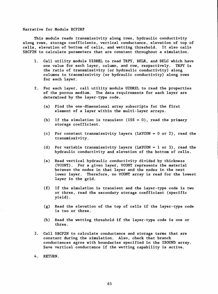
Narrative for Module BCF2RP
This module reads transmissivity along rows, hydraulic conductivity along rows, storage coefficients, vertical conductance, elevation of top of cells, elevation of bottom of cells, and wetting threshold. It also calls SBCF2N to calculate parameters that are constant throughout a simulation.
1. Call utility module U1DREL to read TRPY, DELR, and DELC which have one value for each layer, column, and row, respectively. TRPY is the ratio of transmissivity (or hydraulic conductivity) along columns to transmissivity (or hydraulic conductivity) along rows for each layer.
2. For each layer, call utility module U2DREL to read the properties of the porous medium. The data requirements for each layer are determined by the layer-type code.
(a) Find the one-dimensional array subscripts for the first element of a layer within the multi-layer arrays.
(b) If the simulation is transient (ISS = 0), read the primary storage coefficient.
(c) For constant transmissivity layers (LAYCON = 0 or 2), read the transmissivity.
(d) For variable transmissivity layers (LAYCON = 1 or 3), read the hydraulic conductivity and elevation of the bottom of cells.
(e) Read vertical hydraulic conductivity divided by thickness (VCONT). For a given layer, VCONT represents the material between the nodes in that layer and the nodes in the next lower layer. Therefore, no VCONT array is read for the lowest layer in the grid.
(f) If the simulation is transient and the layer-type code is two or three, read the secondary storage coefficient (specific yield).
(g) Read the elevation of the top of cells if the layer-type code is two or three.
(h) Read the wetting threshold if the layer-type code is one or three.
3. Call SBCF2N to calculate conductance and storage terms that are constant during the simulation. Also, check that branch conductances agree with boundaries specified in the IBOUND array. Save vertical conductance if the wetting capability is active.
4. RETURN.
65

DELR is the grid spacing in the row direc tion.
DELC is the grid spacing in the column direction,
TRPY is the ratio of transmissivity in the column direction to transmissivity in the row direction.
LAYCON is a layer-type code (one for each layer).
0 - confined1 - unconfined2 - confined/unconfined but
transmissivity is constant3 - confined/unconfined
VCONT is vertical hydraulic conductivity divided by distance between the node in one layer and the node in the layer below (one value for each cell in a layer).
WETDRY is the wetting threshold (one value for each cell in a layer).
a>^PC%«<*e
ENTER BCF2RP
IRead DELR, DELC, and
TRPY
1If transient, read primary
storage coefficient
If LAYCON is 0 or 2, read transmissivity
iIf LAYCON is lor 3, readhrdraulic conductivity and
bottom elevation
If not bottom layer, read VCONT
IIf transient and LAYCON is 2 or
3, read secondary storagecoefficient
If LAYCON is 2 or 3, read top elevation
2b
2c
2d
2e
2f
2g
If LAYCON is 1 or 3 and wetting capability is active, read WETDRY
iPrepare and check BCF data
RETURN
FigiireS. -- Flow chart for module BCF2RE
66
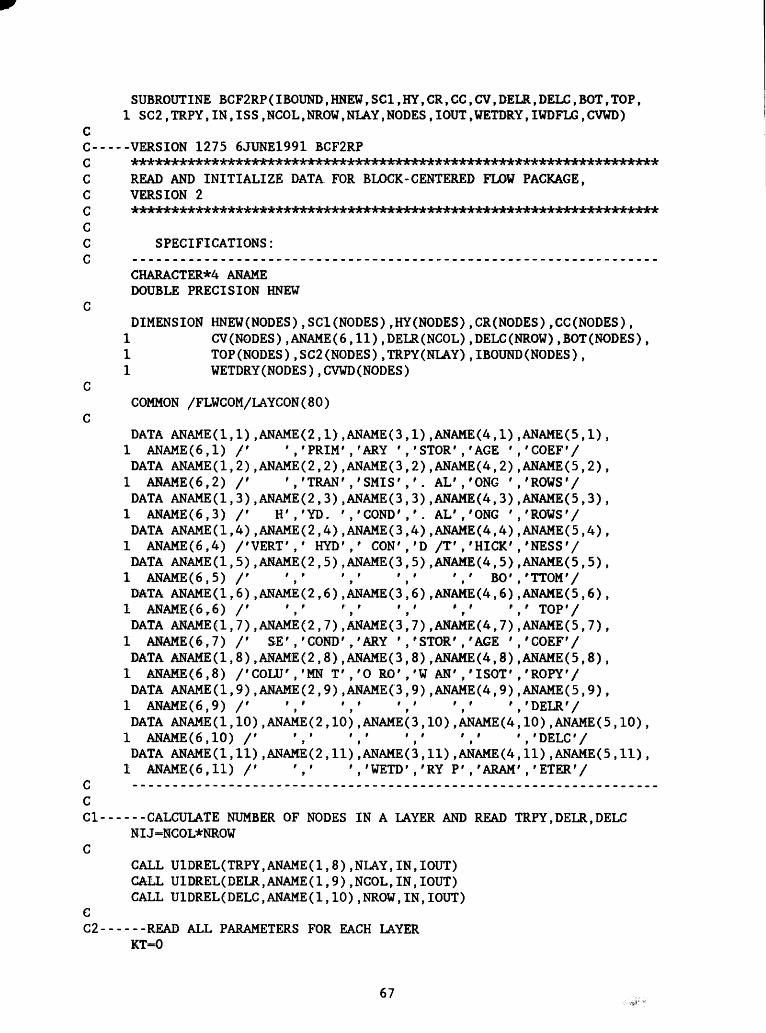
cC-----VERSION 1275 6JUNE1991 BCF2RPC ^*****^:Ht:IHbt**Hr**:IH(r*^^
C READ AND INITIALIZE DATA FOR BLOCK-CENTERED FLOW PACKAGE, C VERSION 2C
_t_^i_^i_ _»_r_ -_ --§_t_ _t_ _t.-i^-i-_ -_ _«-^« »_ ^ -- i_JL^»,^«^, _i.^t_ -_ _ _ _ __ __ --. -_ _. _ ._ __ ._. __ ,- .-_ __ __ -_ .__ > . < »_ __ _ - __ .__ _ TlrxxT«r*x**T^r*TRtx^TRr^?wxxxxTi(r^xTin«^
cC SPECIFICATIONS:C ...................._._......__...................................
CHARACTER*4 ANAME DOUBLE PRECISION KNEW
CDIMENSION HNEW(NODES),SCI(NODES) rHY(NODES),CR(NODES),CC(NODES),
1 CV(NODES),ANAME(6,11).DELR(NCOL).DELC(NROW),BOT(NODES), 1 TOP(NODES),SC2(NODES),TRPY(NLAY),IBOUND(NODES), 1 WETDRY(NODES),CVWD(NODES)
C
CDATA ANAME(1,1),ANAME(2,1),ANAME(3,1),ANAME(4,1),ANAME(5,1),
1 ANAME(6,1) /' ','PRIM','ARY ','STOR','AGE ','COEF'/DATA ANAME(1,2),ANAME(2,2),ANAME(3,2),ANAME(4,2),ANAME(5,2),
1 ANAME(6,2) /' ','TRAN','SMIS','. AL','ONG ','ROWS'/DATA ANAME(1,3),ANAME(2,3),ANAME(3,3),ANAME(4,3),ANAME(5,3),
1 ANAME(6,3) /' H'.'YD. ','COND', r . AL','ONG '/ROWS'/DATA ANAME(1,4),ANAME(2,4),ANAME(3,4),ANAME(4,4),ANAME(5,4),
1 ANAME(6,4) /'VERT',' HYD' ,' CON','D /T','HICK','NESS'/DATA ANAMEU,5),ANAME(2,5),ANAME(3,5),ANAME(4,5),ANAME(5,5),
1 ANAME(6,5) /' ',' ',' ',' ',' BO'/TTOM'/DATA ANAME(l,6),ANAME(2,6),ANAME(3,6),ANAME(4,6) f ANAME(5,6),
1 ANAME(6,6) /' ',' r , f ',' ',' ', r TOP'/DATA ANAME(l,7),ANAME(2,7),ANAME(3,7),ANAME(4,7) f ANAME(5,7),
1 ANAME(6,7) /' SE','COND','ARY ','STOR', rAGE ', r COEF'/DATA ANAME(l,8),ANAME(2,8),ANAME(3,8),ANAME(4,8) f ANAME(5,8) >
1 ANAME(6,8) /'COLU r ,'MN T','0 RO','W AN','ISOT','ROPY'/DATA ANAME(1,9),ANAME(2,9),ANAME(3,9),ANAME(4,9),ANAME(5,9),
1 ANAME(6,9) /' ',' ',' ',' ',' ','DELR'/DATA ANAME(1,10),ANAME(2,10),ANAME(3,10),ANAME(4,10),ANAME(5,10),
1 ANAME(6,10) /' ',' ',' ',' ',' ','DELC'/DATA ANAME(1,11),ANAME(2,11),ANAME(3,11),ANAME(4,11),ANAME(5,11),
1 ANAME(6,11) /' ',' ','WETD','RY P', rARAM','ETER'/ C ...............___..-._._....._..............._.....-............Cd------CALCULATE NUMBER OF NODES IN A LAYER AND READ TRPY,DELR,DELC
NIJ=NCOL*NROW
CC2------READ ALL PARAMETERS FOR EACH LAYER
67
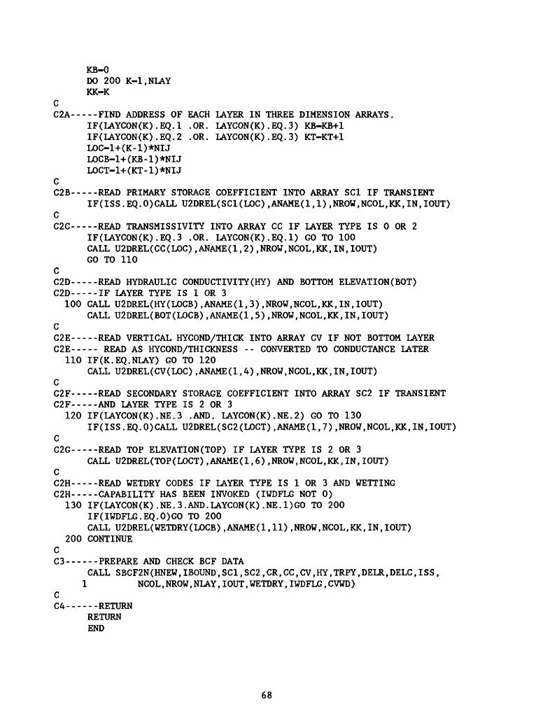
KB-0DO 200 K-l.NLAYKK-K
C C2A-----FIND ADDRESS OF EACH LAYER IN THREE DIMENSION ARRAYS.
IF(LAYCON(K).EQ.l .OR. LAYCON(K).EQ.3) KB-KB+1IF(LAYCON(K).EQ.2 .OR. LAYCON(K).EQ.3) KT-KT+1LOC=1+(K-1)*NIJLOCB-1+(KB-1)*NIJLOCT-1+(KT-1)*NIJ
C C2B-----READ PRIMARY STORAGE COEFFICIENT INTO ARRAY SCI IF TRANSIENT
IF(ISS.EQ.O)CALL U2DREL(SC1(LOC),ANAME(1,1),NROW,NCOL,KK,IN,IOUT) C C2C-----READ TRANSMISSIVITY INTO ARRAY CC IF LAYER TYPE IS 0 OR 2
IF(LAYCON(K).EQ.3 .OR. LAYCON(K).EQ.l) GO TO 100CALL U2DREL(CC(LOC),ANAME(1,2),NROW,NCOL,KK,IN,IOUT)GO TO 110
CC2D-----READ HYDRAULIC CONDUCTIVITY(HY) AND BOTTOM ELEVATION(BOT) C2D-----IF LAYER TYPE IS 1 OR 3
100 CALL U2DREL(HY(LOCB),ANAME(1,3),NROW,NCOL,KK,IN,IOUT)CALL U2DREL(BOT(LOCB),ANAME(1,5),NROW,NCOL,KK,IN,IOUT)
CC2E-----READ VERTICAL HYCOND/THICK INTO ARRAY CV IF NOT BOTTOM LAYER C2E----- READ AS HYCOND/THICKNESS -- CONVERTED TO CONDUCTANCE LATER
110 IF(K.EQ.NLAY) GO TO 120CALL U2DREL(CV(LOC),ANAME(1,4),NROW,NCOL,KK,IN,IOUT)
CC2F-----READ SECONDARY STORAGE COEFFICIENT INTO ARRAY SC2 IF TRANSIENT C2F-----AND LAYER TYPE IS 2 OR 3
120 IF(LAYCON(K).NE.3 .AND. LAYCON(K).NE.2) GO TO 130IF(ISS.EQ.O)CALL U2DREL(SC2(LOCT),ANAME(1,7),NROW,NCOL,KK,IN,IOUT)
C C2G-----READ TOP ELEVATION(TOP) IF LAYER TYPE IS 2 OR 3
CALL U2DREL(TOP(LOCT),ANAME(1,6),NROW,NCOL,KK,IN,IOUT) CC2H-----READ WETDRY CODES IF LAYER TYPE IS 1 OR 3 AND WETTING C2H-----CAPABILITY HAS BEEN INVOKED (IWDFLG NOT 0)
130 IF(LAYCON(K).NE.3.AND.LAYCON(K).NE.1)GO TO 200IF(IWDFLG.EQ.O)GO TO 200CALL U2DREL(WETDRY(LOCB),ANAME(1,11),NROW,NCOL,KK,IN,IOUT)
200 CONTINUE C C3------PREPARE AND CHECK BCF DATA
CALL SBCF2N(KNEW,IBOUND,SCI,SC2,CR,CC,CV,HY,TRPY,DELR,DELC,ISS, 1 NCOL,NROW,NLAY,IOUT,WETDRY,IWDFLG,CVWD)
C C4------RETURN
RETURNEND
68
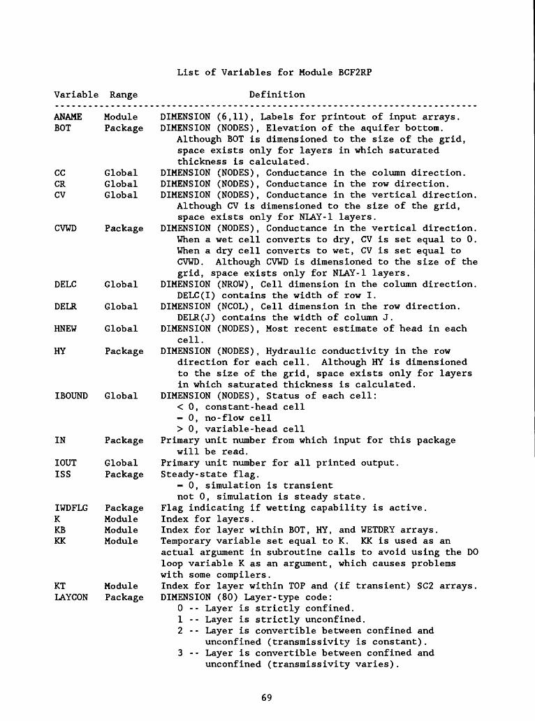
Variable Range
List of Variables for Module BCF2RP
Definition
ANAME Module DIMENSION (6,11), Labels for printout of input arrays.BOT Package DIMENSION (NODES), Elevation of the aquifer bottom.
Although BOT is dimensioned to the size of the grid, space exists only for layers in which saturated thickness is calculated.
CC Global DIMENSION (NODES), Conductance in the column direction.CR Global DIMENSION (NODES), Conductance in the row direction.CV Global DIMENSION (NODES), Conductance in the vertical direction.
Although CV is dimensioned to the size of the grid, space exists only for NLAY-1 layers.
CVWD Package DIMENSION (NODES), Conductance in the vertical direction.When a wet cell converts to dry, CV is set equal to 0. When a dry cell converts to wet, CV is set equal to CWD. Although CVWD is dimensioned to the size of the grid, space exists only for NLAY-1 layers.
DELC Global DIMENSION (NROW), Cell dimension in the column direction.DELC(I) contains the width of row I.
DELR Global DIMENSION (NCOL), Cell dimension in the row direction.DELR(J) contains the width of column J.
KNEW Global DIMENSION (NODES), Most recent estimate of head in eachcell.
HY Package DIMENSION (NODES), Hydraulic conductivity in the rowdirection for each cell. Although HY is dimensioned to the size of the grid, space exists only for layers in which saturated thickness is calculated.
IBOUND Global DIMENSION (NODES), Status of each cell:< 0, constant-head cell- 0, no-flow cell> 0, variable-head cell
IN Package Primary unit number from which input for this packagewill be read.
IOUT Global Primary unit number for all printed output. ISS Package Steady-state flag.
- 0, simulation is transientnot 0, simulation is steady state.
IWDFLG Package Flag indicating if wetting capability is active.K Module Index for layers.KB Module Index for layer within BOT, HY, and WETDRY arrays.KK Module Temporary variable set equal to K. KK is used as an
actual argument in subroutine calls to avoid using the DO loop variable K as an argument, which causes problems with some compilers.
KT Module Index for layer within TOP and (if transient) SC2 arrays.LAYCON Package DIMENSION (80) Layer-type code:
0 -- Layer is strictly confined.1 -- Layer is strictly unconfined.2 - - Layer is convertible between confined and
unconfined (transmissivity is constant).3 -- Layer is convertible between confined and
unconfined (transmissivity varies).
69
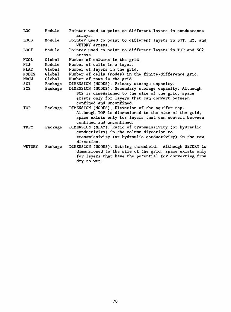
LOG
LOCB
LOCT
TOP
Module
Module
Module
NCOLNIJNIAYNODESNROWSCI SC2
GlobalModuleGlobalGlobalGlobalPackage Package
Package
TRPY Package
WETDRY Package
Pointer used to point to different layers in conductancearrays.
Pointer used to point to different layers in BOT, HY, andWETDRY arrays.
Pointer used to point to different layers in TOP and SC2arrays.
Number of columns in the grid. Number of cells in a layer. Number of layers in the grid.Number of cells (nodes) in the finite-difference grid. Number of rows in the grid.DIMENSION (NODES), Primary storage capacity. DIMENSION (NODES), Secondary storage capacity. Although
SC2 is dimensioned to the size of the grid, spaceexists only for layers that can convert betweenconfined and unconfined.
DIMENSION (NODES), Elevation of the aquifer top.Although TOP is dimensioned to the size of the grid,space exists only for layers that can convert betweenconfined and unconfined.
DIMENSION (NLAY), Ratio of transmissivity (or hydraulicconductivity) in the column direction totransmissivity (or hydraulic conductivity) in the rowdirection.
DIMENSION (NODES), Wetting threshold. Although WETDRY isdimensioned to the size of the grid, space exists onlyfor layers that have the potential for converting fromdry to wet.
70
Narrative for Module BCF2AD
At the beginning of each time step, this module sets head from the previous time step (HOLD) equal to the bottom elevation (EOT) for any cells that are dry and have the potential for converting to wet. This is necessary in order to compute correct storage terms for these cells.
1. Return if steady-state simulation or if the wetting capability is inactive.
2. Loop through all layers to check for dry cells that can become wet.
(a) Keep track of the layer index for wettable layers (layers with layer-type code 1 or 3). Loop through the cells in wettable layers and skip non-wettable layers.
(b) Skip cells that are currently wet (IBOUND not 0) or not wettable (WETDRY - 0).
(c) Set HOLD - EOT.
3. RETURN.
71
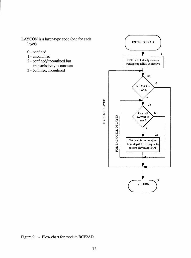
LAYCON is a layer-type code (one for each layer).
0 - confined1 - unconfined2 - confined/unconfined but
transmissivity is constant3 - confined/unconfined
3a u
s
I
ENTER BCF2AD
1
RETURN if steady state or wetting capability is inactive
Can cell X N convert to
wet?
Set head from previoustime step (HOLD) equal to
bottom elevation (EOT)
RETURN
Figure 9. -- Flow chart for module BCF2AD.
72
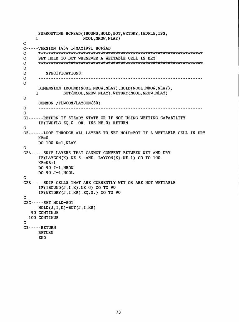
SUBROUTINE BCF2AD(IBOUND,HOLD,BOT,WETDRY,IWDFLG,ISS, 1 NCOL,NROW,NLAY)
C C-----VERSION 1434 14MAY1991 BCF2AD
C SET HOLD TO BOT WHENEVER A WETTABLE CELL IS DRY
CC SPECIFICATIONS:C ..................................................................
CDIMENSION IBOUND(NCOL,NROW,NLAY),HOLD(NCOL,NROW,NLAY),
1 BOT(NCOL,NROW,NLAY),WETDRY(NCOL,NROW,NLAY) C
COMMON /FLWCOM/LAYCON(80) C ..................................................................CCl------RETURN IF STEADY STATE OR IF NOT USING WETTING CAPABILITY
IF(IWDFLG.EQ.O .OR. ISS.NE.O) RETURN C C2------LOOP THROUGH ALL LAYERS TO SET HOLD=BOT IF A WETTABLE CELL IS DRY
KB=0DO 100 K=1,NLAY
C C2A-----SKIP LAYERS THAT CANNOT CONVERT BETWEEN WET AND DRY
IF(LAYCON(K).NE.3 .AND. LAYCON(K).NE.1) GO TO 100KB=KB+1DO 90 I-l.NROWDO 90 J=1,NCOL
C C2B-----SKIP CELLS THAT ARE CURRENTLY WET OR ARE NOT WETTABLE
IF(IBOUND(J,I,K).NE.O) GO TO 90IF(WETDRY(J,I,KB).EQ.O.) GO TO 90
C C2C-----SET HOLD-BOT
HOLD(J,I,K)=BOT(J,I,KB) 90 CONTINUE
100 CONTINUE C C3-----RETURN
RETURNEND
73
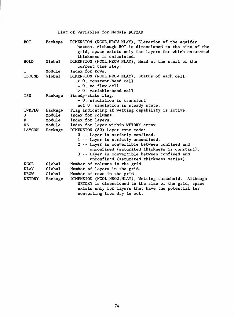
List of Variables for Module BCF2AD
BOT Package DIMENSION (NCOL.NROW.NLAY), Elevation of the aquiferbottom. Although BOT is dimensioned to the size of the grid, space exists only for layers for which saturated thickness is calculated.
HOLD Global DIMENSION (NCOL.NROW.NLAY), Head at the start of thecurrent time step.
I Module Index for rows.IBOUND Global DIMENSION (NCOL.NROW.NLAY), Status of each cell:
< 0, constant-head cell- 0, no-flow cell > 0, variable-head cell
ISS Package Steady-state flag.- 0, simulation is transientnot 0, simulation is steady state.
IWDFLG Package Flag indicating if wetting capability is active. J Module Index for columns. K Module Index for layers.KB Module Index for layer within WETDRY array. LAYCON Package DIMENSION (80) Layer-type code:
0 -- Layer is strictly confined.1 -- Layer is strictly unconfined.2 - - Layer is convertible between confined and
unconfined (saturated thickness is constant).3 - - Layer is convertible between confined and
unconfined (saturated thickness varies). NCOL Global Number of columns in the grid. NLAY Global Number of layers in the grid. NROW Global Number of rows in the grid. WETDRY Package DIMENSION (NCOL.NROW.NLAY), Wetting threshold. Although
WETDRY is dimensioned to the size of the grid, spaceexists only for layers that have the potential forconverting from dry to wet.
74

Narrative for Module BCF2FM
This module calculates branch conductances if they are not constant throughout the simulation, adds storage terms to the HCOF and RHS accumulators, and adds terms to RHS that correct for overestimation of flow down into partially saturated cells.
1. For each layer in which transmissivity varies with head (LAYCON - 1 or 3), call module SBCF2H to calculate branch conductances.
2. If the simulation is transient, calculate storage terms for each layer. Steps 3-5 comprise the storage calculations. If the simulation is steady state, go to Step 6.
3. Determine if the layer is convertible between confined and unconfined.
4. If the layer is not convertible (LAYCON - 0 or 1), use primary storage capacity to calculate storage terms and add them to the right hand side (RHS) and h-coefficient (HCOF) terms.
5. If the layer is convertible (LAYCON - 2 or 3), then use head at the beginning of the time step (HOLD) to determine the storage factor at the beginning of the time step (SOLD). Use the latest estimate of head at the end of the time step (KNEW) to determine the storage factor at the end of the time step (SNEW). Note that the term "storage factor" as used in BCF2FM refers to storage capacity divided by time step length. Use SOLD and SNEW to calculate storage terms and add them to RHS and HCOF.
6. For each layer, determine if correction terms are needed forvertical flow down into a partially saturated layer (Steps 7-8).
7. If the layer is partially saturated and there is flow from above, calculate the vertical flow correction terms and add them to RHS (program comment C7D). This vertical flow correction is incorporated jointly in RHS and HCOF in the original model (McDonald and Harbaugh, 1988, p. 5-23 and 5-59). In BCF2, the correction is being made through RHS alone in order to avoid the possibility of producing a matrix that is not diagonally dominant. A non-diagonally dominant matrix causes problems with the Preconditioned Conjugate-Gradient Package, version 2 (Hill, 1990, p. 15). Implementing the correction through RHS alone is essentially equivalent to the former method. The method using both RHS and HCOF is an implicit representation of the correction while the method using only RHS is an explicit representation.
8. If this layer is not the bottom layer and the layer below ispartially saturated, calculate the correction terms and add them to RHS.
9. RETURN.
75

LAYCON is a layer-type code (one for each layer).
0 - confined1 - unconfined2 - confined/unconfined but
transmissivity is constant3 - confined/unconfined
c ENTER BCF2FM
FOR EACH LAYER\ F
If T varies, calcu late horizontal conductances
1
Add storage to flow equa tion primary storage
only
Add storage to flowequation may be a
combination of primaryand secondary storage
If LAYCON is 2 or 3, add correction term for flow from above if applicable
If LAYCON for layer below is 2 or 3, add cor rection term for flow to
below if applicable
RETURN
Figure 10. -- Flow chart for module BCF2FM.
76
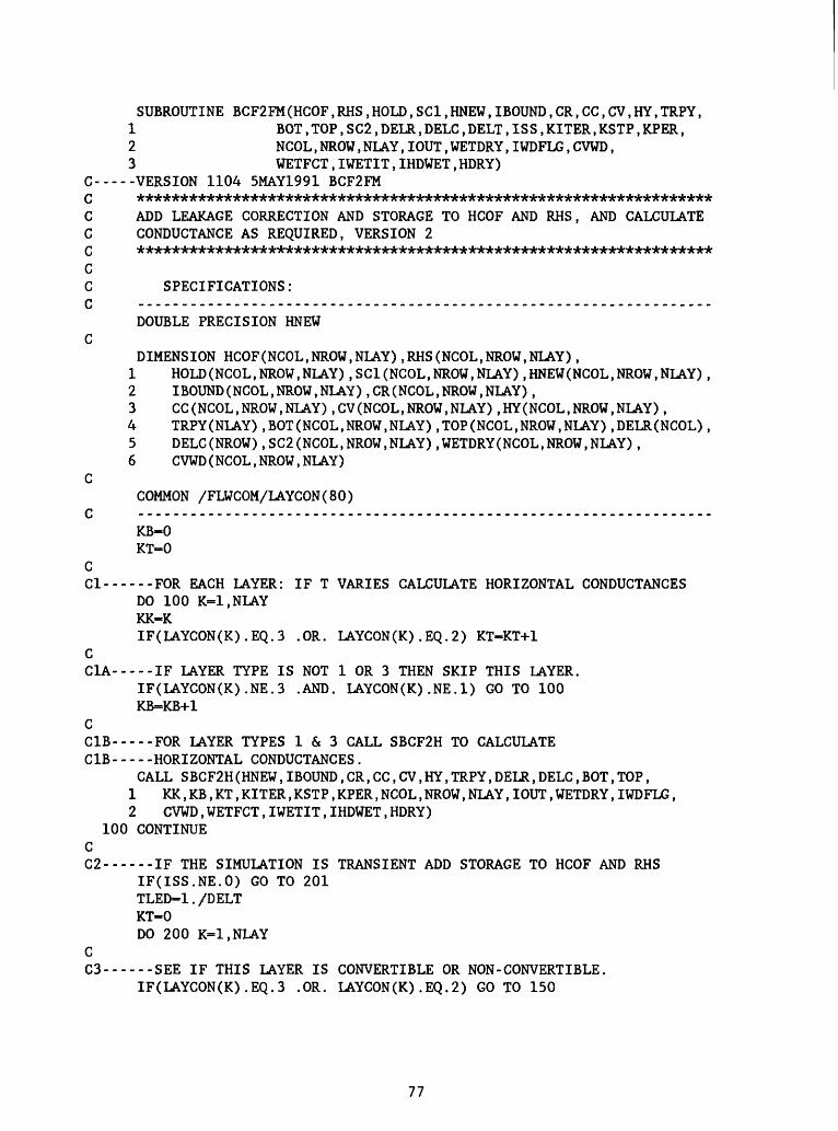
SUBROUTINE BCF2FM(HCOF,RHS,HOLD,SCI,KNEW,IBOUND,CR,CC,CV,HY,TRPY,1 BOT,TOP,SC2,DELR,DELC,DELT,IS S,KITER,KSTP,KPER,2 NCOL,NROW,NLAY,IOUT,WETDRY,IWDFLG,CVWD,3 WETFCT,IWETIT,IHDWET,HDRY)
C-..--VERSION 1104 5MAY1991 BCF2FM
C ADD LEAKAGE CORRECTION AND STORAGE TO HCOF AND RHS, AND CALCULATE C CONDUCTANCE AS REQUIRED, VERSION 2
CC SPECIFICATIONS:C ..................................................................
DOUBLE PRECISION KNEW C
DIMENSION HCOF(NCOL,NROW,NLAY),RHS(NCOL,NROW,NLAY),1 HOLD(NCOL,NROW,NLAY),SCI(NCOL,NROW,NLAY), KNEW(NCOL,NROW,NLAY),2 IBOUND(NCOL,NROW,NLAY),CR(NCOL,NROW,NLAY),3 CC(NCOL,NROW,NLAY),CV(NCOL,NROW,NLAY),HY(NCOL,NROW,NLAY),4 TRPY(NLAY),BOT(NCOL,NROW,NLAY),TOP(NCOL,NROW,NLAY),DELR(NCOL),5 DELC(NROW),SC2(NCOL,NROW,NLAY).WETDRY(NCOL,NROW,NLAY),6 CVWD(NCOL,NROW,NLAY)
CCOMMON /FLWCOM/LAYCON(80)
C ..................................................................KB-0KT-0
C C1------FOR EACH LAYER: IF T VARIES CALCULATE HORIZONTAL CONDUCTANCES
DO 100 K=1,NLAYKK-KIF(LAYCON(K).EQ.3 .OR. LAYCON(K).EQ.2) KT-KT+1
C C1A-----IF LAYER TYPE IS NOT 1 OR 3 THEN SKIP THIS LAYER.
IF(LAYCON(K).NE.3 .AND. LAYCON(K).NE.1) GO TO 100KB-KB+1
CC1B-----FOR LAYER TYPES 1 & 3 CALL SBCF2H TO CALCULATE C1B-----HORIZONTAL CONDUCTANCES.
CALL SBCF2H(KNEW,IBOUND,CR,CC,CV,HY,TRPY,DELR,DELC,BOT,TOP,1 KK,KB,KT,KITER,KSTP,KPER,NCOL,NROW,NLAY,IOUT,WETDRY,IWDFLG,2 CVWD,WETFCT,IWETIT,IHDWET,HDRY)
100 CONTINUE C C2------IF THE SIMULATION IS TRANSIENT ADD STORAGE TO HCOF AND RHS
IF(ISS.NE.O) GO TO 201TLED-1./DELTKT-0DO 200 K=1,NLAY
C C3------SEE IF THIS LAYER IS CONVERTIBLE OR NON-CONVERTIBLE.
IF(LAYCON(K).EQ.3 .OR. LAYCON(K).EQ.2) GO TO 150
77
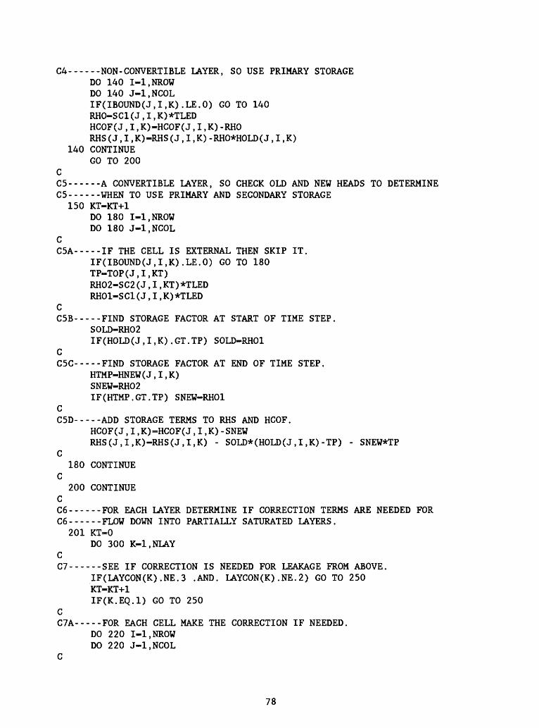
C4------NON-CONVERTIBLE LAYER, SO USE PRIMARY STORAGEDO 140 I-l.NROWDO 140 J-l.NCOLIF(IBOUND(J,I,K).LE.O) GO TO 140RHO-SC1(J,I,K)*TLEDHCOF(J,I,K)-HCOF(J,I,K)-RHORHS(J,I,K)-RHS(J,I,K)-RHO*HOLD(J,I,K)
140 CONTINUEGO TO 200
C C5------A CONVERTIBLE LAYER, SO CHECK OLD AND NEW HEADS TO DETERMINEC5------WHEN TO USE PRIMARY AND SECONDARY STORAGE
150 KT-KT+1DO 180 I-l.NROWDO 180 J-l.NCOL
C C5A-----IF THE CELL IS EXTERNAL THEN SKIP IT.
IF(IBOUND(J,I,K).LE.O) GO TO 180TP-TOP(J,I,KT)RH02-SC2(J,I,KT)*TLEDRH01-SC1(J,I,K)*TLED
C C5B-----FIND STORAGE FACTOR AT START OF TIME STEP.
SOLD-RH02IF(HOLD(J,I,K).GT.TP) SOLD-RH01
C C5C-----FIND STORAGE FACTOR AT END OF TIME STEP.
HTMP-HNEW(J,I,K)SNEW-RH02IF(HTMP.GT.TP) SNEW-RH01
C C5D-----ADD STORAGE TERMS TO RHS AND HCOF.
HCOF(J,I,K)=HCOF(J,I,K)-SNEWRHS(J,I,K)-RHS(J,I,K) - SOLD*(HOLD(J,I,K)-TP) - SNEW*TP
C180 CONTINUE
C200 CONTINUE
C C6------FOR EACH LAYER DETERMINE IF CORRECTION TERMS ARE NEEDED FORC6------FLOW DOWN INTO PARTIALLY SATURATED LAYERS.
201 KT=0DO 300 K-1,NLAY
C C7...... SEE IF CORRECTION IS NEEDED FOR LEAKAGE FROM ABOVE.
IF(LAYCON(K).NE.3 .AND. LAYCON(K).NE.2) GO TO 250KT-KT+1IF(K.EQ.l) GO TO 250
C C7A-----FOR EACH CELL MAKE THE CORRECTION IF NEEDED.
DO 220 I-l.NROWDO 220 J-l.NCOL
C
78

C7B-----IF THE CELL IS EXTERNAL(IBOUNEK-0) THEN SKIP IT.IF(IBOUND(J,I,K).LE.O) GO TO 220HTMP=HNEW(J,I,K)
C C7C-----IF HEAD IS ABOVE TOP THEN CORRECTION NOT NEEDED
IF(HTMP.GE.TOP(J,I,KT)) GO TO 220 C C7D-----WITH HEAD BELOW TOP ADD CORRECTION TERMS TO RHS.
RHS(J,I,K)=RHS(J,I,K) + CV(J,I,K-1)*(TOP(J,1,KT)-HTMP) 220 CONTINUE
C C8------SEE IF THIS LAYER MAY NEED CORRECTION FOR LEAKAGE TO BELOW.
250 IF(K.EQ.NLAY) GO TO 300IF(LAYCON(K+1).NE.3 .AND. LAYCON(K+1).NE.2) GO TO 300KTT-KT+1
C C8A-----FOR EACH CELL MAKE THE CORRECTION IF NEEDED.
DO 280 I=1,NROWDO 280 J=1,NCOL
C C8B-----IF CELL IS EXTERNAL (IBOUNEK=0) THEN SKIP IT.
IF(IBOUND(J,I,K).LE.O) GO TO 280 CC8C-----IF HEAD IN THE LOWER CELL IS LESS THAN TOP ADD CORRECTION C8C-----TERM TO RHS.
HTMP-HNEW(J,I,K+1)IF(HTMP.LT.TOP(J,I,KTT)) RHS(J,1,K)=RHS(J,I,K)
1 - CV(J,I,K)*(TOP(J,I,KTT)-HTMP) 280 CONTINUE 300 CONTINUE
C C9------RETURN
RETURNEND
79
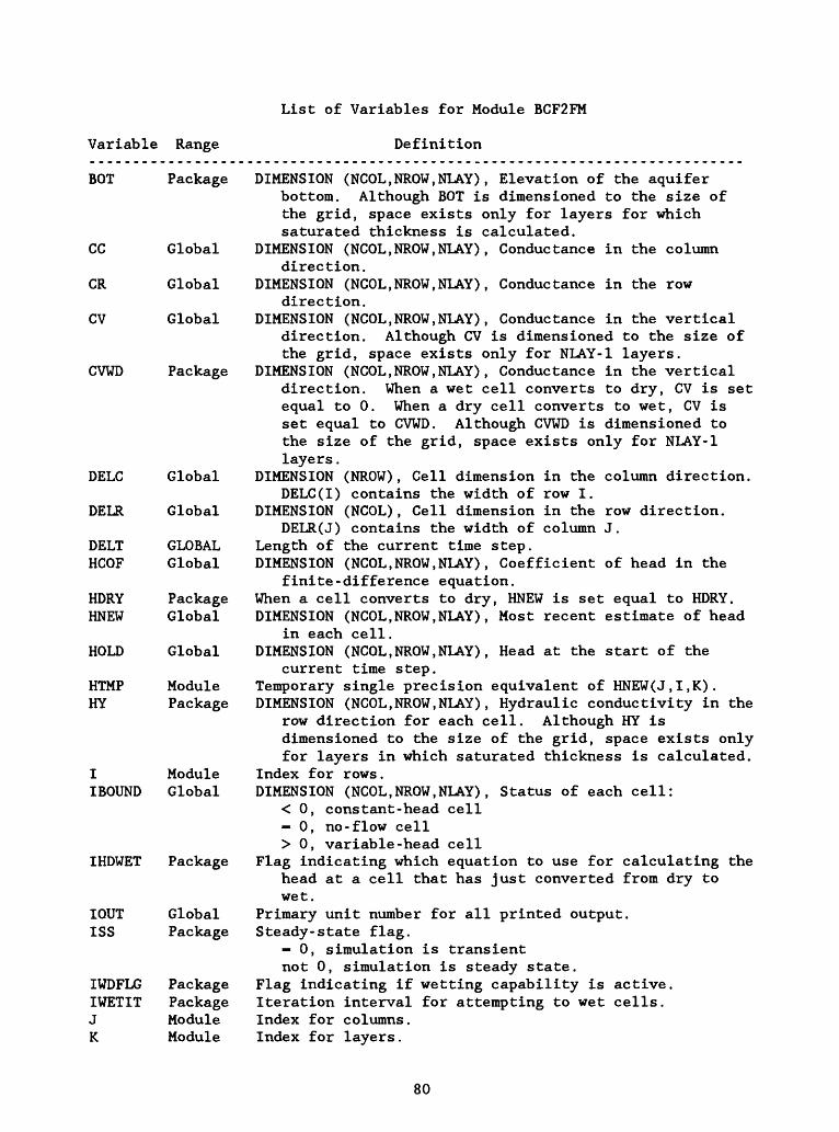
List of Variables for Module BCF2FM
Variable Range
EOT Package
CC Global
CR Global
CV Global
Definition
CVWD
DELC
DELR
DELT HCOF
HDRYHNEW
HOLD
HTMP HY
IOUT ISS
Package
DIMENSION (NCOL,NROW,NLAY), Elevation of the aquifer bottom. Although EOT is dimensioned to the size of the grid, space exists only for layers for which saturated thickness is calculated.
DIMENSION (NCOL,NROW,NLAY), Conductance in the column direction.
DIMENSION (NCOL,NROW,NLAY), Conductance in the row direction.
DIMENSION (NCOL,NROW,NLAY), Conductance in the vertical direction. Although CV is dimensioned to the size of the grid, space exists only for NLAY-1 layers.
DIMENSION (NCOL,NROW,NLAY), Conductance in the vertical direction. When a wet cell converts to dry, CV is set equal to 0. When a dry cell converts to wet, CV is set equal to CVWD. Although CVWD is dimensioned to the size of the grid, space exists only for NLAY-1 layers.
DIMENSION (NROW), Cell dimension in the column direction. DELC(I) contains the width of row I.
DIMENSION (NCOL), Cell dimension in the row direction. DELR(J) contains the width of column J.
Length of the current time step.DIMENSION (NCOL,NROW,NLAY), Coefficient of head in the
finite-difference equation.When a cell converts to dry, HNEW is set equal to HDRY.DIMENSION (NCOL,NROW,NLAY), Most recent estimate of head
in each cell.DIMENSION (NCOL,NROW,NLAY), Head at the start of the
current time step.Temporary single precision equivalent of HNEW(J,I,K).DIMENSION (NCOL,NROW,NLAY), Hydraulic conductivity in the
row direction for each cell. Although HY is dimensioned to the size of the grid, space exists only for layers in which saturated thickness is calculated.
Index for rows.DIMENSION (NCOL,NROW,NLAY), Status of each cell:
< 0, constant-head cell- 0, no-flow cell> 0, variable-head cell
Flag indicating which equation to use for calculating thehead at a cell that has just converted from dry towet.
Primary unit number for all printed output. Steady-state flag.
0, simulation is transientnot 0, simulation is steady state.
Flag indicating if wetting capability is active. Iteration interval for attempting to wet cells. Index for columns. Index for layers.
Global
Global
GLOBAL Global
Package Global
Global
Module Package
I Module IBOUND Global
IHDWET Package
Global Package
IWDFLG PackageIWETIT PackageJ ModuleK Module
80
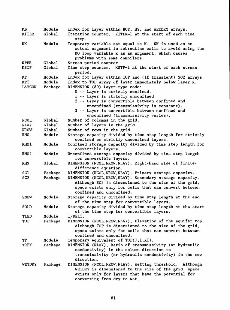
KB KITER
KK
KPER KSTP
NCOL NLAY NROW RHO
RH01
RH02
RHS
SCI SC2
SNEW
SOLD
TIED TOP
TP TRPY
Module Global
Module
Global Global
KT ModuleKIT ModuleLAYCON Package
Global Global Global Module
Module
Module
Global
Package Package
Module
Module
Module Package
Module Package
WETDRY Package
Index for layer within BOT, HY, and WETDRY arrays. Iteration counter. KITER-1 at the start of each time
step. Temporary variable set equal to K. KK is used as an
actual argument in subroutine calls to avoid using theDO loop variable K as an argument, which causesproblems with some compilers.
Stress period counter. Time step counter. KSTP-1 at the start of each stress
period.Index for layer within TOP and (if transient) SC2 arrays. Index to TOP array of layer immediately below layer K. DIMENSION (80) Layer-type code:
0 -- Layer is strictly confined.1 -- Layer is strictly unconfined.2 - - Layer is convertible between confined and
unconfined (transmissivity is constant).3 - - Layer is convertible between confined and
unconfined (transmissivity varies). Number of columns in the grid. Number of layers in the grid. Number of rows in the grid. Storage capacity divided by time step length for strictly
confined or strictly unconfined layers. Confined storage capacity divided by time step length for
convertible layers. Unconfined storage capacity divided by time step length
for convertible layers.DIMENSION (NCOL,NROW,NLAY), Right-hand side of finite-
difference equation.DIMENSION (NCOL,NROW,NLAY), Primary storage capacity. DIMENSION (NCOL,NROW,NLAY), Secondary storage capacity.
Although SC2 is dimensioned to the size of the grid,space exists only for cells that can convert betweenconfined and unconfined.
Storage capacity divided by time step length at the endof the time step for convertible layers.
Storage capacity divided by time step length at the startof the time step for convertible layers.
1/DELT. DIMENSION (NCOL,NROW,NLAY), Elevation of the aquifer top.
Although TOP is dimensioned to the size of the grid,space exists only for cells that can convert betweenconfined and unconfined.
Temporary equivalent of TOP(J,I,KT). DIMENSION (NLAY), Ratio of transmissivity (or hydraulic
conductivity) in the column direction totransmissivity (or hydraulic conductivity) in the rowdirection.
DIMENSION (NCOL,NROW,NLAY), Wetting threshold. AlthoughWETDRY is dimensioned to the size of the grid, spaceexists only for layers that have the potential forconverting from dry to wet.
81

WETFCT Package A factor that is included in the calculation of the headthat is established at a cell that has just converted from dry to wet.
82
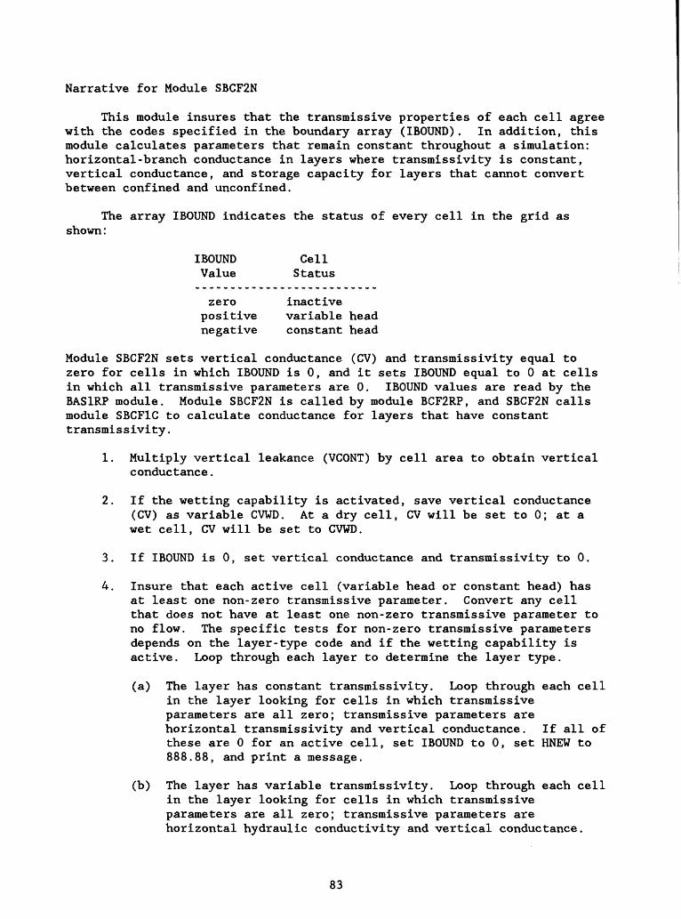
Narrative for Module SBCF2N
This module insures that the transmissive properties of each cell agree with the codes specified in the boundary array (IBOUND). In addition, this module calculates parameters that remain constant throughout a simulation: horizontal-branch conductance in layers where transmissivity is constant, vertical conductance, and storage capacity for layers that cannot convert between confined and unconfined.
The array IBOUND indicates the status of every cell in the grid as shown:
IBOUND Value
zero positive negative
Cell Status
inactive variable head constant head
Module SBCF2N sets vertical conductance (CV) and transmissivity equal to zero for cells in which IBOUND is 0, and it sets IBOUND equal to 0 at cells in which all transmissive parameters are 0. IBOUND values are read by the BAS1RP module. Module SBCF2N is called by module BCF2RP, and SBCF2N calls module SBCF1C to calculate conductance for layers that have constant transmi s s ivi ty.
1. Multiply vertical leakance (VCONT) by cell area to obtain vertical conductance.
2. If the wetting capability is activated, save vertical conductance (CV) as variable CVWD. At a dry cell, CV will be set to 0; at a wet cell, CV will be set to CVWD.
3. If IBOUND is 0, set vertical conductance and transmissivity to 0.
4. Insure that each active cell (variable head or constant head) has at least one non-zero transmissive parameter. Convert any cell that does not have at least one non-zero transmissive parameter to no flow. The specific tests for non-zero transmissive parameters depends on the layer-type code and if the wetting capability is active. Loop through each layer to determine the layer type.
(a) The layer has constant transmissivity. Loop through each cell in the layer looking for cells in which transmissive parameters are all zero', transmissive parameters are horizontal transmissivity and vertical conductance. If all of these are 0 for an active cell, set IBOUND to 0, set KNEW to 888.88, and print a message.
(b) The layer has variable transmissivity. Loop through each cell in the layer looking for cells in which transmissive parameters are all zero; transmissive parameters are horizontal hydraulic conductivity and vertical conductance.
83

(1) If the wetting capability is active for a cell, check to see if CVWD above or below is non zero. The test for non-zero CVWD is performed even if the cell is initially dry because the cell could convert to wet at a later time, and this would be senseless if all transmissive terms were zero.
(2) For active cells in which the wetting capability is not active, check to see if CV above or below is non zero.
(3) For cells in which CV or CVWD above and below are zero, check to see if hydraulic conductivity is zero.
(4) Hydraulic conductivity and vertical conductance above and below are all zero, so convert the cell to no flow. Set IBOUND to 0, set KNEW to 888.88, and print a message. Also, if the wetting capability is active, set WETDRY to 0 so that the cell is never allowed to become wet.
5. Call module SBCF1C to calculate conductance for layers that have constant transmissivity.
6. If a transient simulation, loop through each layer and calculate storage capacity as the product of storage coefficient and cell area.
(a) Calculate primary storage capacity for all layers.
(b) For layers that can convert between confined and unconfined, calculate secondary storage capacity.
7. RETURN.
84
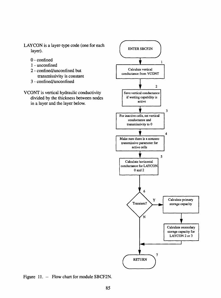
LAYCON is a layer-type code (one for each layer).
0 - confined1 - unconfined2 - confined/unconfined but
transmissivity is constant3 - confined/unconfined
VCONT is vertical hydraulic conductivity divided by the thickness between nodes in a layer and the layer below.
ENTER SBCF2N
ICalculate vertical
conductance from VCONT
Save vertical conductanceif wetting capability is
active
For inactive cells, set vertical conductance and
transmissivity to 0
Make sure there is a nonzerotransmissive parameter for
active cells
Calculate horizontal conductance for LAYCON
Oand2
1
/Tram
\
P 6Vient? X __
/N
*+
i _ ̂ i
^ Calculate primary storage capacity
|Calculate secondary storage capacity for
LAYCON 2 or 3
1
RETURN
Figure 11. -- Flow chart for module SBCF2N.
85
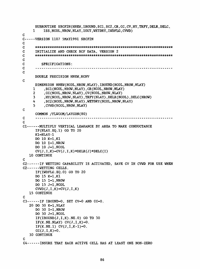
SUBROUTINE SBCF2N(HNEW,IBOUND,SCI,SC2,CR,CC,CV,HY,TRPY,DELR,DELC, 1 IS S,NCOL,NROW,NLAY,IOUT,WETDRY,IWDFLG,CVWD)
CC-----VERSION 1107 5MAY1991 SBCF2N C CC INITIALIZE AND CHECK BCF DATA, VERSION 2 C C C SPECIFICATIONS:
DOUBLE PRECISION HNEW,HCNV C
DIMENSION HNEW(NCOL,NROW,NLAY),IBOUND(NCOL,NROW,NLAY)1 ,SCI(NCOL,NROW,NLAY),CR(NCOL,NROW,NLAY)2 ,CC(NCOL,NROW,NLAY),CV(NCOL,NROW,NLAY)3 ,HY(NCOL, NROW, NLAY) ,TRPY(NLAY) ,DELR(NCOL) , DELC (NROW)4 ,SC2(NCOL,NROW,NLAY),WETDRY(NCOL,NROW,NLAY)5 ,CVWD(NCOL,NROW,NLAY)
CCOMMON /FLWCOM/LAYCON(80)
C ..................................................................CCl------MULTIPLY VERTICAL LEAKANCE BY AREA TO MAKE CONDUCTANCE
IF(NLAY.EQ.l) GO TO 20K1=NLAY-1DO 10 K=1,K1DO 10 1=1,NROWDO 10 J-1,NCOLCV(J,I,K)=CV(J,I,K)*DELR(J)*DELC(I)
10 CONTINUE C C2------IF WETTING CAPABILITY IS ACTIVATED, SAVE CV IN CVWD FOR USE WHENC2------WETTING CELLS.
IF(IWDFLG.EQ.O) GO TO 20DO 15 K=1,K1DO 15 1=1,NROWDO 15 J=1,NCOLCVWD(J,I,K)-CV(J,I,K)
15 CONTINUE C C3------IF IBOUND=0, SET CV=0 AND CC=0.
20 DO 30 K=1,NLAYDO 30 1=1,NROWDO 30 J-1,NCOLIF(IBOUND(J,I,K).NE.O) GO TO 30IF(K.NE.NLAY) CV(J,I,K)=0.IF(K.NE.l) CV(J,I,K-1)=0.CC(J,I,K)=0.
30 CONTINUE C C4------INSURE THAT EACH ACTIVE CELL HAS AT LEAST ONE NON-ZERO
86
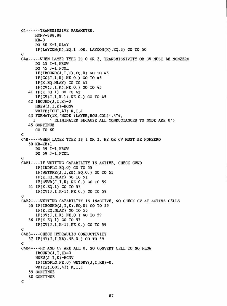
C4------TRANSMIS SIVE PARAMETER.HCNV-888.88KB=0DO 60 K-l.NLAYIF(LAYCON(K).EQ.l .OR. LAYCON(K).EQ.3) GO TO 50
C C4A-----WHEN LAYER TYPE IS 0 OR 2, TRANSMISSIVITY OR CV MUST BE NONZERO
DO 45 I-l.NROWDO 45 J-l.NCOLIF(IBOUND(J,I,K).EQ.O) GO TO 45IF(CC(J,I,K).NE.O.) GO TO 45IF(K.EQ.NLAY) GO TO 41IF(CV(J,I,K).NE.O.) GO TO 45
41 IF(K.EQ.l) GO TO 42IF(CV(J,I,K-1).NE.O.) GO TO 45
42 IBOUND(J,I,K)=0 HNEW(J,I,K)=HCNV WRITE(IOUT,43) K,I,J
43 FORMAT(IX,'NODE (LAYER,ROW,COL)',314,1 ' ELIMINATED BECAUSE ALL CONDUCTANCES TO NODE ARE 0')
45 CONTINUE GO TO 60
C C4B-----WHEN LAYER TYPE IS 1 OR 3, HY OR CV MUST BE NONZERO
50 KB-KB+1DO 59 I-l.NROWDO 59 J-l.NCOL
C C4B1----IF WETTING CAPABILITY IS ACTIVE, CHECK CVWD
IF(IWDFLG.EQ.O) GO TO 55IF(WETDRY(J,I,KB).EQ.O.) GO TO 55IF(K.EQ.NLAY) GO TO 51IF(CVWD(J,I,K).NE.O.) GO TO 59
51 IF(K.EQ.l) GO TO 57IF(CV(J,I,K-1).NE.O.) GO TO 59
C C4B2----WETTING CAPABILITY IS INACTIVE, SO CHECK CV AT ACTIVE CELLS
55 IF(IBOUND(J,I,K).EQ.O) GO TO 59 IF(K.EQ.NLAY) GO TO 56 IF(CV(J,I,K).NE.O.) GO TO 59
56 IF(K.EQ.l) GO TO 57IF(CV(J,I,K-1).NE.O.) GO TO 59
C C4B3----CHECK HYDRAULIC CONDUCTIVITY
57 IF(HY(J,I,KB).NE.O.) GO TO 59 C C4B4----HY AND CV ARE ALL 0, SO CONVERT CELL TO NO FLOW
IBOUND(J,I,K)-0HNEW(J,I,K)=HCNVIF(IWDFLG.NE.O) WETDRY(J,1,KB)-0.WRITE(IOUT,43) K,I,J
59 CONTINUE60 CONTINUE
C
87
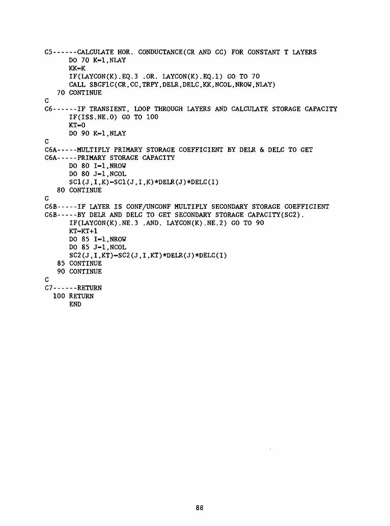
C5------CALCULATE HOR. CONDUCTANCE(CR AND CC) FOR CONSTANT T LAYERSDO 70 K-l.NLAYKK-KIF(LAYCON(K).EQ.3 .OR. LAYCON(K).EQ.l) GO TO 70CALL SBCFIC(CR,CC,TRPY,DELR,DELC,KK,NCOL,NROW,NLAY)
70 CONTINUE C C6------IF TRANSIENT, LOOP THROUGH LAYERS AND CALCULATE STORAGE CAPACITY
IF(ISS.NE.O) GO TO 100KT-0DO 90 K-l.NLAY
CC6A-----MULTIPLY PRIMARY STORAGE COEFFICIENT BY DELR & DELC TO GET C6A-----PRIMARY STORAGE CAPACITY
DO 80 1=1,NROWDO 80 J-l.NCOLSC1(J,I,K)=SC1(J,I,K)*DELR(J)*DELC(I)
80 CONTINUE CC6B-----IF LAYER IS CONF/UNCONF MULTIPLY SECONDARY STORAGE COEFFICIENT C6B-----BY DELR AND DELC TO GET SECONDARY STORAGE CAPACITY(SC2).
IF(LAYCON(K).NE.3 .AND. LAYCON(K).NE.2) GO TO 90KT-KT+1DO 85 1=1,NROWDO 85 J=1,NCOLSC2(J,I,KT)-SC2(J,I,KT)*DELR(J)*DELC(I)
85 CONTINUE 90 CONTINUE
C C7------RETURN
100 RETURNEND
88
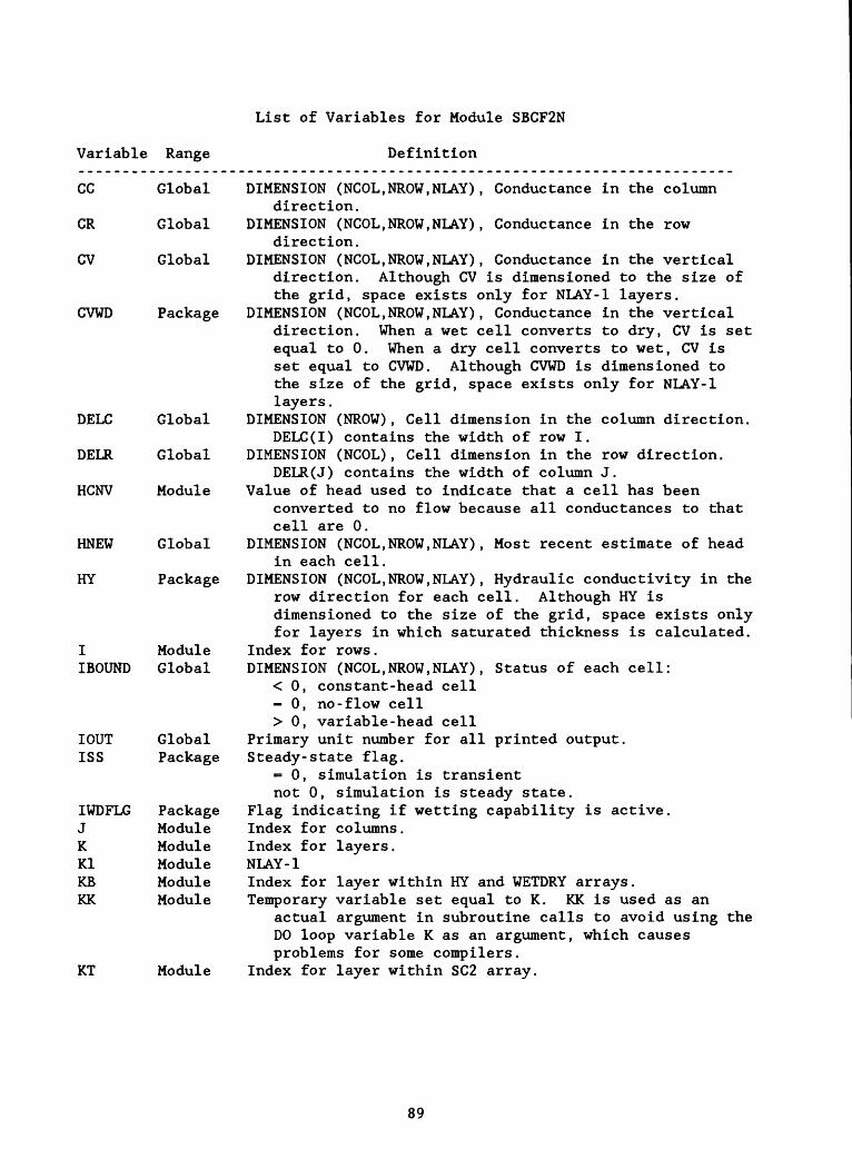
List of Variables for Module SBCF2N
Variable Range
CC Global
CR Global
CV Global
Definition
DELC Global
DELR Global
HCNV Module
DIMENSION (NCOL,NROW,NLAY), Conductance in the columndirection.
DIMENSION (NCOL,NROW,NLAY), Conductance in the rowdirection.
DIMENSION (NCOL,NROW,NLAY), Conductance in the verticaldirection. Although CV is dimensioned to the size ofthe grid, space exists only for NLAY-1 layers.
CVWD Package DIMENSION (NCOL,NROW,NLAY), Conductance in the verticaldirection. When a wet cell converts to dry, CV is setequal to 0. When a dry cell converts to wet, CV isset equal to CVWD. Although CVWD is dimensioned tothe size of the grid, space exists only for NLAY-1layers.
DIMENSION (NROW), Cell dimension in the column direction.DELC(I) contains the width of row I.
DIMENSION (NCOL), Cell dimension in the row direction.DELR(J) contains the width of column J.
Value of head used to indicate that a cell has beenconverted to no flow because all conductances to thatcell are 0.
HNEW Global DIMENSION (NCOL,NROW,NLAY), Most recent estimate of headin each cell.
HY Package DIMENSION (NCOL,NROW,NLAY), Hydraulic conductivity in therow direction for each cell. Although HY isdimensioned to the size of the grid, space exists onlyfor layers in which saturated thickness is calculated.
Index for rows. DIMENSION (NCOL,NROW,NLAY), Status of each cell:
< 0, constant-head cell= 0, no-flow cell> 0, variable-head cell
IOUT Global Primary unit number for all printed output. ISS Package Steady-state flag.
= 0, simulation is transientnot 0, simulation is steady state.
IWDFLG Package Flag indicating if wetting capability is active. J Module Index for columns. K Module Index for layers. Kl Module NLAY-1KB Module Index for layer within HY and WETDRY arrays. KK Module Temporary variable set equal to K. KK is used as an
actual argument in subroutine calls to avoid using theDO loop variable K as an argument, which causesproblems for some compilers.
KT Module Index for layer within SC2 array.
I Module IBOUND Global
89
LAYCON Package DIMENSION (80) Layer-type code:0 -- Layer is strictly confined.1 -- Layer is strictly unconfined.2 -- Layer is convertible between confined and
unconfined (transmissivity is constant).3 -- Layer is convertible between confined and
unconfined (transmissivity varies). NCOL Global Number of columns in the grid. NLAY Global Number of layers in the grid. NROW Global Number of rows in the grid.SCI Package DIMENSION (NCOL,NROW,NLAY), Primary storage capacity. SC2 Package DIMENSION (NCOL,NROW,NLAY), Secondary storage capacity.
Although SC2 is dimensioned to the size of the grid,space exists only for cells that can convert betweenconfined and unconfined.
TRPY Package DIMENSION (NLAY), Ratio of transmissivity (or hydraulicconductivity) in the column direction totransmissivity (or hydraulic conductivity) in the rowdirection.
WETDRY Package DIMENSION (NCOL,NROW,NLAY), Wetting threshold. AlthoughWETDRY is dimensioned to the size of the grid, spaceexists only for layers that have the potential forconverting from dry to wet.
90

Narrative for Module SBCF2H
Module SBCF2H calculates the horizontal-branch conductances for a layer in which the transmissivity is a function of head. It does this by calculating transmissivity for each cell as saturated thickness times hydraulic conductivity. Then it calls module SBCF1C to calculate the conductances from transmissivity of cells. As part of saturated thickness calculations, module SBCF2H determines if dry cells should become wet or if wet cells should become dry. Module BCF2FM calls SBCF2H for each type 1 or type 3 layer at each iteration.
1. Loop through each cell in the layer, and calculate transmissivity at each active cell. Before starting, initialize several variables. NCNVRT keeps track of the number of cells that have converted between wet and dry since the last line was printed telling which cells have converted. A line of output may list up to 8 cell conversions. IHDCNV controls the printing of the cell conversion heading; this heading is printed the first time a line of cell conversions is printed. ITFLG is 0 if the attempt to wet cells should be made this iteration, which means that the wetting capability is active and the current iteration is an even multiple of the wetting iteration interval (IWETIT).
2. If the cell is active, go to the saturated thickness calculation.
3. When the cell is inactive, check for the possibility of wetting. A cell has the potential for converting to wet only if ITFLG is zero. Also, the wetting threshold must be non zero. If these conditions are not met, go to the code that sets transmissivity to zero. If these conditions are met, calculate the turn-on threshold, TURNON, and continue the process of determining whether the cell should be converted to wet.
(a) Check the cell below the inactive cell to see if it isvariable head and if the wetting threshold has been reached. If so, go to the code that converts the cell to wet. Note that a constant head cell cannot cause another cell to become wet.
(b) If the wetting threshold is negative, do not make any further attempts to wet the cell; the cell remains dry, and transmissivity will be set to zero. If the wetting threshold is positive, check the four horizontal neighbors to see if the turn-on threshold is reached. Neighboring cells that have converted to wet during the current iteration are not allowed to cause a cell to convert to wet. This is implemented by temporarily setting IBOUND to 30000 in Step 4 when a cell becomes wet. That is, neighboring cells having IBOUND of 30000 are not checked to see if the turn-on threshold is reached. If the turn-on threshold is reached, go to the code that converts the cell to wet.
(c) The cell will stay dry. Set transmissivity to 0, and go to the end of the cell loop.
91

4. The cell becomes wet. Set initial head according to the flagIHDWET, set vertical conductance to CVWD, and set IBOUND to 30000. IBOUND will later be set to 1, but it is momentarily set to a high value as a flag to indicate cells that have been converted to wet this iteration. The flag is used in Step 3b to prevent a newly converted cell from causing other cells to convert. This could otherwise cause a chain reaction.
(a) Save the information about which cell has converted to wet so that it can be printed. When eight conversions between wet and dry have been accumulated, print a line listing those cells.
5. Calculate saturated thickness. If LAYCON is 3, saturated thickness has a maximum value of TOP-BOT.
6. Check to see if saturated thickness is less than 0.
(a) Saturated thickness is greater than 0; calculatetransmissivity as saturated thickness times hydraulic conductivity. Store transmissivity temporarily in CC. Go to the end of the cell loop.
(b) Saturated thickness is less than or equal to 0; convert the cell to no flow and save information flagging which cell has converted to dry. When eight conversions between wet and dry have been accumulated, print a line listing those cells. If the cell is not constant head, set IBOUND, CC (transmissivity), and CV to 0. If the cell is constant head, stop the simulation.
7. Transmissivity has been calculated for all cells. If there is a partially filled line of output of cell conversions, print the line.
8. Convert IBOUND values of 30000 to 1.
9. Call module SBCF1C to calculate conductance from transmissivity.
10. RETURN.
92

KH
dw uK U
OS
£
Is cellallowed to
becomewet?
Y
Calculate saturated thickness
Set initial head andvertical conductance
in cell
6b
Calculate transmissivity
Convert cell to dry transmissivity = 0
iChange boundary code
for cells that converted towet
ICalculate horizontal branch conductances
10RETURN
Figure 12. -- Flow chart for module SBCF2H.
93
i 3c
Transmissivity = 0
J
SUBROUTINE SBCF2H(HNEW,IBOUND,CR,CC,CV,HY,TRPY,DELR,DELC1.BOT,TOP,K,KB,KT,KITER,KSTP,KPER,NCOL,NROW,NLAY,IOUT2.WETDRY,IWDFLG,CVWD,WETFCT,IWETIT,IHDWET,HDRY)
C-----VERSION 1345 23MAY1991 SBCF2H C C *****************************************************************^C COMPUTE CONDUCTANCE FOR ONE LAYER FROM SATURATED THICKNESS ANDC HYDRAULIC CONDUCTIVITY, VERSION 2C *****************************************************************^CC SPECIFICATIONS:C .........................._........._.............................
DOUBLE PRECISION KNEW C
DIMENSION HNEW(NCOL,NROW,NLAY),IBOUND(NCOL,NROW,NLAY)1.CR(NCOL,NROW,NLAY), CC(NCOL,NROW,NLAY), CV(NCOL,NROW,NLAY)2.HY(NCOL,NROW,NLAY), TRPY(NLAY), DELR(NCOL), DELC(NROW)3.BOT(NCOL,NROW,NLAY),TOP(NCOL,NROW,NLAY),WETDRY(NCOL,NROW,NLAY)4.CVWD(NCOL,NROW,NLAY)CHARACTER*4 ACNVRTDIMENSION ICNVRT(8),JCNVRT(8),ACNVRT(8)
CCOMMON /FLWCOM/LAYCON(80)
C ......._..._.._...........__..._..._...__._.......................CCl-.-..-LOOP THROUGH EACH CELL IN LAYER AND CALCULATE TRANSMISSIVITY ATC1------EACH ACTIVE CELL.
NCNVRT=0IHDCNV-0ITFLG=1IF(IWDFLG.NE.O) ITFLG=MOD(KITER,IWETIT)DO 200 1=1,NROWDO 200 J=1,NCOL
C C2------IF CELL IS ACTIVE, THEN SKIP TO CODE THAT CALCULATES SATURATEDC2------THICKNESS.
IF(IBOUND(J,I,K).NE.O) GO TO 20 C C3------DETERMINE IF THE CELL CAN CONVERT BETWEEN CONFINED ANDC3------UNCONFINED. IF NOT, SKIP TO CODE THAT SETS TRANSMISSIVITY TO 0
IF(ITFLG.NE.O) GO TO 6IF(WETDRY(J,I,KB).EQ.O.O)GO TO 6WD=WETDRY(J,I,KB)IF(WD.LT.O.) WD=-WDTURNON=BOT(J,I,KB)+WD
CC3A-----CHECK HEAD IN CELL BELOW TO SEE IF WETTING THRESHOLD HAS BEEN C3A-----REACHED.
IF(K.EQ.NLAY)GO TO 2HTMP=HNEW(J,I,K+1)IF(IBOUND(J,I,K+1).GT.O.AND.HTMP.GE.TURNON)GO TO 9
C C3B-----CHECK HEAD IN ADJACENT HORIZONTAL CELLS TO SEE IF WETTING
94
C3B-----THRESHOLD HAS BEEN REACHED.2 IF(WETDRY(J,I,KB).LT.O.) GO TO 6
IF(J.EQ.1)GO TO 3 HTMP-HNEW(J-1,I,K)IF(IBOUND(J-1,I,K).GT.O.AND.IBOUND(J-1,I,K).NE.30000.AND.
1 HTMP.GE.TURNON)GO TO 93 IF(J.EQ.NCOL)GO TO 4 HTMP-HNEW( J-f-1,1, K) IF(IBOUND(J+1,I,K).GT.O.AND.HTMP.GE.TURNON)GO TO 9
4 IF(I.EQ.1)GO TO 5 HTMP-HNEW(J,I-1,K)IF(IBOUND(J,I-1,K).GT.O.AND.IBOUND(J,I-1,K).NE.30000.AND.
1 HTMP.GE.TURNON)GO TO 95 IF(I.EQ.NROW)GO TO 6HTMP-HNEW(J,I+1,K)IF(IBOUND(J,I-f-l,K).GT.O.AND.HTMP.GE.TURNON)GO TO 9
CC3C-----CELL IS DRY AND STAYS DRY. SET TRANSMISSIVITY TO 0 AND SKIP C3C-----TO THE NEXT CELL.
6 CC(J,I,K)-0.GO TO 200
C C4------CELL BECOMES WET. SET INITIAL HEAD AND VERTICAL CONDUCTANCE.
9 IF(IHDWET.NE.O) HNEW(J,I,K)-BOT(J,I,KB)+WETFCT*WDIF(IHDWET.EQ.0) HNEW(J,I,K)-BOT(J,I,KB)+WETFCT*(HTMP-BOT(J,I,KB)) IF(K.EQ.NLAY) GO TO 12IF(IBOUND(J,I,K+1).NE.O) CV(J,I,K)- CVWD(J,I,K)
12 IF(K.EQ.l) GO TO 14IF(IBOUND(J,I,K-1).NE.O) CV(J,I,K-1)- CVWD(J,I,K-1)
14 IBOUND(J,I,K)-30000 C C4A-----PRINT MESSAGE SAYING CELL HAS BEEN CONVERTED TO WET.
NCNVRT-NCNVRT+1 ICNVRT(NCNVRT)=I JCNVRT(NCNVRT)=J ACNVRT(NCNVRT)=' WET' IF(NCNVRT.LT.S) GO TO 20
IF(IHDCNV.EQ.O) WRITE(IOUT,17) KITER,K,KSTP,KPER17 FORMAT(1HO,'CELL CONVERSIONS FOR ITERATION-',13,' LAYER-',
1 12,' TIME STEP-',13,' STRESS PERIOD-',13,' (ROW,COL)') IHDCNV-1 WRITE(IOUT,18) (ACNVRT(L),ICNVRT(L),JCNVRT(L),L-1,NCNVRT)
18 FORMAT(1X,8(A4,'(',13,',',13, ' ) '))NCNVRT-0
C C5------CALCULATE SATURATED THICKNESS.
20 HD-HNEW(J,I,K)IF(LAYCON(K).EQ.l) GO TO 50 IF(HD.GT.TOP(J,I,KT)) HD-TOP(J,I,KT)
50 THCK=HD-BOT(J,I,KB) C C6------CHECK TO SEE IF SATURATED THICKNESS IS GREATER THAN ZERO.
IF(THCK.LE.O.) GO TO 100 C
95

C6A-----IF SATURATED THICKNESS>0 THEN TRANSMISSIVITY IS HYDRAULIC C6A-----CONDUCTIVITY TIMES SATURATED THICKNESS.
CC(J,I,K)-THCK*HY(J,I,KB) GO TO 200
CC6B-----WHEN SATURATED THICKNESS < 0, PRINT A MESSAGE AND SET C6B-----TRANSMISSIVITY, IBOUND, AND VERTICAL CONDUCTANCE -0
100 NCNVRT-NCNVRT+1 ICNVRT(NCNVRT)-! JCNVRT(NCNVRT)-J ACNVRT(NCNVRT)-' DRY' IF(NCNVRT.LT.8) GO TO 150
IF(IHDCNV.EQ.O) WRITE(IOUT,17) KITER,K,KSTP,KPERIHDCNV-1WRITE(IOUT,18) (ACNVRT(L),ICNVRT(L),JCNVRT(L),L-1,NCNVRT)NCNVRT-0
150 HNEW(J,I,K)-HDRY CC(J,I,K)-0.IF(IBOUND(J,I,K).GE.O) GO TO 160
WRITE(IOUT,151)151 FORMAT(1HO,'CONSTANT-HEAD CELL WENT DRY -- SIMULATION ABORTED')
WRITE(IOUT,152) K,I,J,KITER,KSTP,KPER152 FORMAT(1X,'LAYER-',12,' ROW-',13,' COLUMN-',13,
1 ' ITERATION-',13,' TIME STEP-',13,' STRESS PERIOD-',13)STOP
160 IBOUND(J,I,K)-0IF(K.LT.NLAY) CV(J,I,K)=0. IF(K.GT.l) CV(J,I,K-1)-0.
200 CONTINUE C C7------PRINT ANY REMAINING CELL CONVERSIONS NOT YET PRINTED
IF(NCNVRT.EQ.O) GO TO 203IF(IHDCNV.EQ.O) WRITE(IOUT,17) KITER,K,KSTP,KPER IHDCNV-1WRITE(IOUT,18) (ACNVRT(L),ICNVRT(L),JCNVRT(L),L-1.NCNVRT) NCNVRT-0
C C8------CHANGE IBOUND VALUE FOR CELLS THAT CONVERTED TO WET THISC8------ITERATION FROM 30000 to 1.
203 IF(IWDFLG.EQ.O) GO TO 210 DO 205 I-l.NROW DO 205 J-l.NCOLIF(IBOUND(J,I,K).EQ.30000) IBOUND(J,I,K)-1
205 CONTINUE C C9------COMPUTE HORIZONTAL BRANCH CONDUCTANCES FROM TRANSMISSIVITY.
210 CALL SBCF1C(CR,CC,TRPY,DELR,DELC,K,NCOL,NROW,NLAY) C CIO-----RETURN
RETURN END
96

List of Variables for Module SBCF2H
Variable Range
ACNVRT Module
BOT Package
Definition
CVWD Package
DIMENSION (8), Contains "DRY" or "WET" for up to eightcells that have converted between wet and dry.
DIMENSION (NCOL,NROW,NLAY), Elevation of the aquifer bottom. Although BOT is dimensioned to the size of the grid, space exists onlfor cells for which saturated thickness is calculated.
CC Global DIMENSION (NCOL,NROW,NLAY), Conductance in the columndirection. This array is also used to temporarily hold saturated thickness.
CR Global DIMENSION (NCOL,NROW,NLAY), Conductance in the rowdirection.
CV Global DIMENSION (NCOL,NROW,NLAY), Conductance in the verticaldirection. Although CV is dimensioned to the size of the grid, space exists only for NLAY-1 layers.
DIMENSION (NCOL,NROW,NLAY), Conductance in the vertical direction. When a wet cell converts to dry, CV is set equal to 0. When a dry cell converts to wet, CV is set equal to CWD. Although CVWD is dimensioned to the size of the grid, space exists only for NLAY-1 layers.
DELC Global DIMENSION (NROW), Cell dimension in the column direction.DELC(I) contains the width of row I.
DELR Global DIMENSION (NCOL), Cell dimension in the row direction.DELR(J) contains the width of column J.
HD Module Single precision equivalent of HNEW(J,I,K). HDRY Package When a cell converts to dry, HNEW is set equal to HDRY. HNEW Global DIMENSION (NCOL,NROW,NLAY), Most recent estimate of head
in each cell.Temporary single precision equivalent of HNEW. Index for rows.DIMENSION (NCOL,NROW,NLAY), Status of each cell:
< 0, constant-head cell = 0, no-flow cell > 0, variable-head cell
DIMENSION (8), Row index for up to eight cells that haveconverted between wet and dry.
Flag indicating if any cell conversion information hasbeen printed.
Flag indicating which equation to use for calculating the head at a cell that has just converted from dry to wet.
IOUT Global Primary unit number for all printed output. ITFLG Module Flag indicating if the current iteration is one in which
cells are allowed to convert from dry to wet. Flag indicating if wetting capability is active. Iteration interval for attempting to wet cells. Index for columns. DIMENSION (8), Column index for up to eight cells that
have converted between wet and dry. K Module Index for layers.
HTMP ModuleI ModuleIBOUND Global
ICNVRT Module
IHDCNV Module
IHDWET Package
IWDFLG PackageIWETIT PackageJ ModuleJCNVRT Module
97

KB KITER
KPER KSTP
TRPY
TURNONWDWETDRY
Module Global
Global Global
KT ModuleL ModuleLAYCON Package
NCNVRT Module
NCOLNLAYNROWTHCKTOP
GlobalGlobalGlobalModulePackage
Package
Module Module Package
WETFCT Package
Index for layer within BOT, HY, and WETDRY arrays. Iteration counter. KITER-1 at the start of each time
step.Stress period counter. Time step counter. KSTP-1 at the start of each stress
period.Index for layer within TOP array. Index for printing cell conversion information. DIMENSION (80) Layer-type code:
0 -- Layer is strictly confined.1 -- Layer is strictly unconfined.2 - - Layer is convertible between confined and
unconfined (transmissivity is constant).3 -- Layer is convertible between confined and
unconfined (transmissivity varies). Counter for number of cells that have converted between
wet and dry since a line of conversion information hasbeen printed.
Number of columns in the grid. Number of layers in the grid. Number of rows in the grid. Saturated thickness. DIMENSION (NCOL,NROW,NLAY), Elevation of the aquifer top.
Although TOP is dimensioned to the size of the grid,space exists only for cells that can convert betweenconfined and unconfined.
DIMENSION (NLAY), Ratio of transmissivity (or hydraulicconductivity) in the column direction totransmissivity (or hydraulic conductivity) in the rowdirection.
Turn-on threshold.The absolute value of WETDRY(J,I,KB). DIMENSION (NCOL,NROW,NLAY), Wetting threshold. Although
WETDRY is dimensioned to the size of the grid, spaceexists only for layers that have the potential forconverting from dry to wet.
A factor that is included in the calculation of the headthat is established at a cell that has just convertedfrom dry to wet.
98
REFERENCES CITED
American National Standards Institute, 1978, Programming language FORTRAN:
American National Standards Institute, X3.9-1978, 18 ch.
Hill, M. C., 1990, Preconditioned conjugate-gradient 2 (PCG2), a computer
program for solving ground-water flow equations: U.S. Geological Survey
Water-Resources Investigations Report 90-4048, 43 p.
Kuiper, L. K., 1987, Computer program for solving ground-water flow
equations by the preconditioned conjugate gradient method: U.S.
Geological Survey Water-Resources Investigations Report 87-4091, 34 p.
McDonald, M. G. and Harbaugh, A. W., 1988, A modular three-dimensional
finite-difference ground-water flow model: U.S. Geological Survey
Techniques of Water Resources Investigations, Book 6, Chapter Al,
586 p.
99