a method to construct dose–response curves for a wide

Journal of Experimental Botany, Vol. 61, No. 8, pp. 2043–2055, 2010doi:10.1093/jxb/erp358 Advance Access publication 4 January, 2010

REVIEW PAPER

A method to construct dose–response curves for a widerange of environmental factors and plant traits by means ofa meta-analysis of phenotypic data

Hendrik Poorter1,2,*, Ulo Niinemets3, Achim Walter1, Fabio Fiorani4 and Uli Schurr1

1 ICG-3 (Phytosphare), Forschungszentrum Julich, D-52425 Julich, Germany2 Ecophysiology of Plants, Institute of Environmental Biology, PO Box 800.84, 3508 TB Utrecht, The Netherlands3 Department of Plant Physiology, Institute of Agricultural and Environmental Sciences, Estonian University of Life Sciences,Kreutzwaldi 1, Tartu 51014, Estonia4 CropDesign NV, Technologiepark 3, B-9052 Zwijnaarde, Belgium

* To whom correspondence should be addressed. E-mail: [email protected]

Received 27 July 2009; Revised 27 October 2009; Accepted 2 November 2009

Abstract

In the past, biologists have characterized the responses of a wide range of plant species to their environment. As

a result, phenotypic data from hundreds of experiments are publicly available now. Unfortunately, this information is

not structured in a way that enables quantitative and comparative analyses. We aim to fill this gap by building a large

database which currently contains data on 1000 experiments and 800 species. This paper presents methodology to

generalize across different experiments and species, taking the response of specific leaf area (SLA; leaf area:leaf

mass ratio) to irradiance as an example. We show how to construct and quantify a normalized mean light–response

curve, and subsequently test whether there are systematic differences in the form of the curve between contrastingsubgroups of species. This meta-analysis is then extended to a range of other environmental factors important for

plant growth as well as other phenotypic traits, using >5300 mean values. The present approach, which we refer to

as ‘meta-phenomics’, represents a valuable tool in understanding the integrated response of plants to their

environment and could serve as a benchmark for future phenotyping efforts as well as for modelling global change

effects on both wild species and crops.

Key words: Biomass allocation, dry matter percentage, environment, meta-phenomics, plasticity, response curve, specific leaf

area.

Introduction

The last 100 years have seen a substantial increase in efforts

invested in plant biology research, and an even greater rise

in the number of scientific publications documenting the

outcome of these efforts. While the first investigations ofbotanists focused on the analysis of plants growing in an

agricultural setting or in their natural habitat (Kreusler,

1879; Hanson, 1917), gradually the research focus has

shifted to include pot-grown plants raised in experimental

gardens or glasshouses. Although this allowed for a more

standardized supply of nutrients and water, such plants still

experience strong variation of light and temperature over

the day, from day to day, and across seasons, complicating

comparisons across experiments. The use of plant growth

chambers enabled an even better control of the environ-mental conditions in which the plants were grown and

allowed them to be challenged with a reproducible environ-

ment (Went, 1957). In this way, the effect of a range of

environmental factors on the growth and development of

plants could be studied, by comparing two or more test

groups exposed to the same target set of environmental

Abbreviations: DMC, dry matter content; DPI, daily photon irradiance; LMF, leaf mass fraction; SLA, specific leaf area; SMF, stem mass fraction; RMF, root massfraction.ª The Author [2010]. Published by Oxford University Press [on behalf of the Society for Experimental Biology]. All rights reserved.For Permissions, please e-mail: [email protected]

at Forschungszentrum

Juelich, Zentralbibliothek on July 5, 2011

jxb.oxfordjournals.orgD

ownloaded from

http://jxb.oxfordjournals.org/

conditions except for the factor(s) of interest (Evans et al.,

1985).

Thousands of experiments have been carried out in these

different settings, and an amazing variety of plant species

have been tested for their response to a suite of environ-

mental conditions. With the increasing number of published

data sets, the necessity arose to summarize results and

generalize from case studies to broad-scale patterns. Thefirst attempts to produce a synthesis of the published

research consisted of an expert-based description. Scientists

working in a certain area outlined general trends by

combining information from a range of publications and

presenting these in a generally narrative way. This ap-

proach, which has proven valuable up to today, allows for

a flexible form of reviewing and emphasizes paradigms and

patterns considered of major significance by leading experts.However, narrative reviews could potentially suffer from

drawbacks. They focus mainly on qualitative (i.e. direction-

ality of response) rather than on quantitative differences

and they may contain varying levels of subjective judge-

ment, as it is almost impossible for the authors not to

express their personal view. Although conceivable, it is hard

to devise standardized procedures for this traditional form

of review.The last 30 years have seen the development of a more

quantitative approach to reviewing a certain research area,

in the form of so-called ‘meta-analyses’ (Hedges and Olkin,

1985). This type of analysis aims at generalizing in a formal

way across a number of independent experiments. To this

end, a suitable effect–size metric is defined, for example the

value of the variable of interest measured in environment A

divided by its value in environment B (Osenberg et al., 1997;Hedges et al., 1999). Following such an approach, the

response of various plant traits to specific environmental

factors has been analysed [e.g. Searles et al. (2001) for UV-

B; Morgan et al. (2003) for ozone; Poorter and Navas

(2003) for CO2]. Meta-analyses, carefully restricted to

discrete treatment levels, such as the effect of elevated CO2

in the 600–800 lmol mol�1 range compared with a baseline

level in the 300–400 lmol mol�1 range, may give a syntheticoverview of the response of plants to the expected doubling

of the CO2 concentration. As such, they can provide

a focused answer to practical questions, such as the effect

of global change on agricultural productivity in 50 years

time, taking the current situation as a baseline. However,

nearly all environmental factors that affect plant growth are

intrinsically continuous variables, and we would gain much

better insight into a plant’s physiology if we account for thisby generating overall response curves. The most basic

questions would then be whether the response is positive or

negative, and whether there are any non-linearities (De

Groot et al., 2002). From the archetypical response curves

as described by Mitscherlich (1909) for nutrients, we know

that such non-linearities may well occur and, in some cases,

their modelling has advanced our understanding signifi-

cantly (Farquhar et al., 2001). Unfortunately, for manyplant traits we have as yet no proper insight into the exact

form of the response curve.

A second goal of a systematic analysis of the literature

that could significantly advance our understanding of plant

responses to their environment is the quantitative parame-

terization of such response curves. Quantifying general

relationships for a given plant trait—or a combination of

traits—across the full range of environmental conditions in

which plants generally occur could not only improve

ecological models of global change effects, but could alsobe valuable for breeders to predict the phenotypic perfor-

mance in environments of varying complexity. A good

example is the analysis of Wright et al. (2004), who

described quantitative relationships between leaf morphol-

ogy, photosynthetic capacity and leaf nitrogen across

a wide range of wild species growing in their natural

habitat. These quantitative estimates have been subse-

quently used to develop further theory on the relationshipbetween growth and nitrogen uptake as observed in the

laboratory (Hikosaka and Osone, 2009). An additional

asset to the quantification of response curves across a wide

variety of experiments with an array of plant species is

that it would allow the establishment of ‘normal limits’.

The concept of normal limits is used advantageously in the

medical field as a guide to doctors with respect to the

normally expected biological variation for a trait acrosshealthy persons (Bezemer et al., 1982). Observed values

beyond these limits do not necessarily indicate serious

illness, but are a reason for increased awareness. We

believe that the establishment of normal limits could be

similarly helpful in plant biology. It could serve as an early

warning for scientists that plants in their experiments are

‘off’ because of unwanted effects, for example a failure in

the temperature regulation of the growth room, that haveescaped their attention. Having excluded such a possibility,

the definition of normal limits could also serve as

a quantitative handle to show that a given plant species

shows specialized adaptations to its environment, different

from most other plant species.

A third goal of such an analysis is to analyse retrospec-

tively whether variation in the response to the environment

can be ascribed to differences in the experimental design, orto differences between functional groups of species. In the

case of elevated CO2, such an approach has been fruitfully

used to show that plants grown in small pots were restricted

in their response to CO2 (Arp, 1991) and that C4 species,

although responding less strongly than C3 species, nonethe-

less increase biomass at elevated CO2 concentrations

(Poorter, 1993). Highly relevant questions that have re-

ceived little attention so far, for example, are: (i) to whatextent is the form of the response curve determined by the

cultivation system (outdoor, glasshouses, or in growth

chambers); (ii) to what extent is the form of the response

curve phylogenetically constrained and; (iii) do ecologically

different groups of species respond differently? Although

the literature is rich in data documenting a wide variety of

stress experiments, plant species, and traits, specific groups

of species and phenotypic traits have received moreattention than others. An additional result of this type of

analysis can be directed awareness about potential gaps in

2044 | Poorter et al. at F

orschungszentrum Juelich, Z

entralbibliothek on July 5, 2011jxb.oxfordjournals.org

Dow

nloaded from


our knowledge that could result in concerted efforts in

prioritizing certain types of experiments.

Taking into account the above considerations, we set

out to devise an approach that could generalize data

across a range of experiments by constructing dose–response

curves in a quantitative manner, enabling comparisons across

different environmental factors as well as a range of

phenotypic traits. After an introduction to this procedure inthe next section, we exemplify the method by comparing the

response of an important growth-related trait, SLA (specific

leaf area), across 12 different environmental factors. Finally,

by comparing light–response curves of SLA, biomass alloca-

tion, and the dry mass:fresh mass ratio we show how this

approach can be successfully scaled up to encompass a wide

range of plant traits. We propose to name the methodology

where this specific method of meta-analysis is used todescribe the phenome of the plant as ‘meta-phenomics’.

A method to calculate generalized responsecurves

To infer proper response curves for a specific organismpreferably requires five or more different levels of a given

environmental factor over the range that plants are likely to

encounter. Although such experiments occasionally have

been carried out (MacDowall, 1972; Van de Vijver et al.,

1993; Juurola, 2003), the large majority of papers we

reviewed (>85%) focused on two or three levels at most.

How then can we generalize across such data?

A way to achieve this goal is to construct response curvesby combining information from various experiments. To this

end, we set out to produce a large compilation of literature

data on experiments with individually grown plants, sub-

jected to the experimental manipulation of one or more

environmental factors. In the case of multiple factors, experi-

ments were only considered when treatments were applied

fully factorially. This compilation currently consists of 1000

experiments, with observations on >800 different species.

To construct response curves from such a database is notstraightforward, because experiments have been conducted

under widely different conditions, using many different

species. A proper analysis requires an appropriate scaling

of both the environmental factor (on the x-axis) and the

plant response variable (on the y-axis). We achieve this goal

using a three-step procedure, which we illustrate by

constructing the response curve of SLA (m2 leaf kg�1 leaf

dry matter) as dependent on the available light during plantgrowth. The SLA determines how much light-intercepting

leaf area is made given a certain plant biomass investment

in leaves, and is as such one of the key factors for the

growth of plants (Lambers and Poorter, 1992). It is a widely

used plant trait in a range of fields, from plant physiology

to ecology (Roumet et al., 1996; Wright et al., 2004). To

exemplify the procedure, we start with literature data for

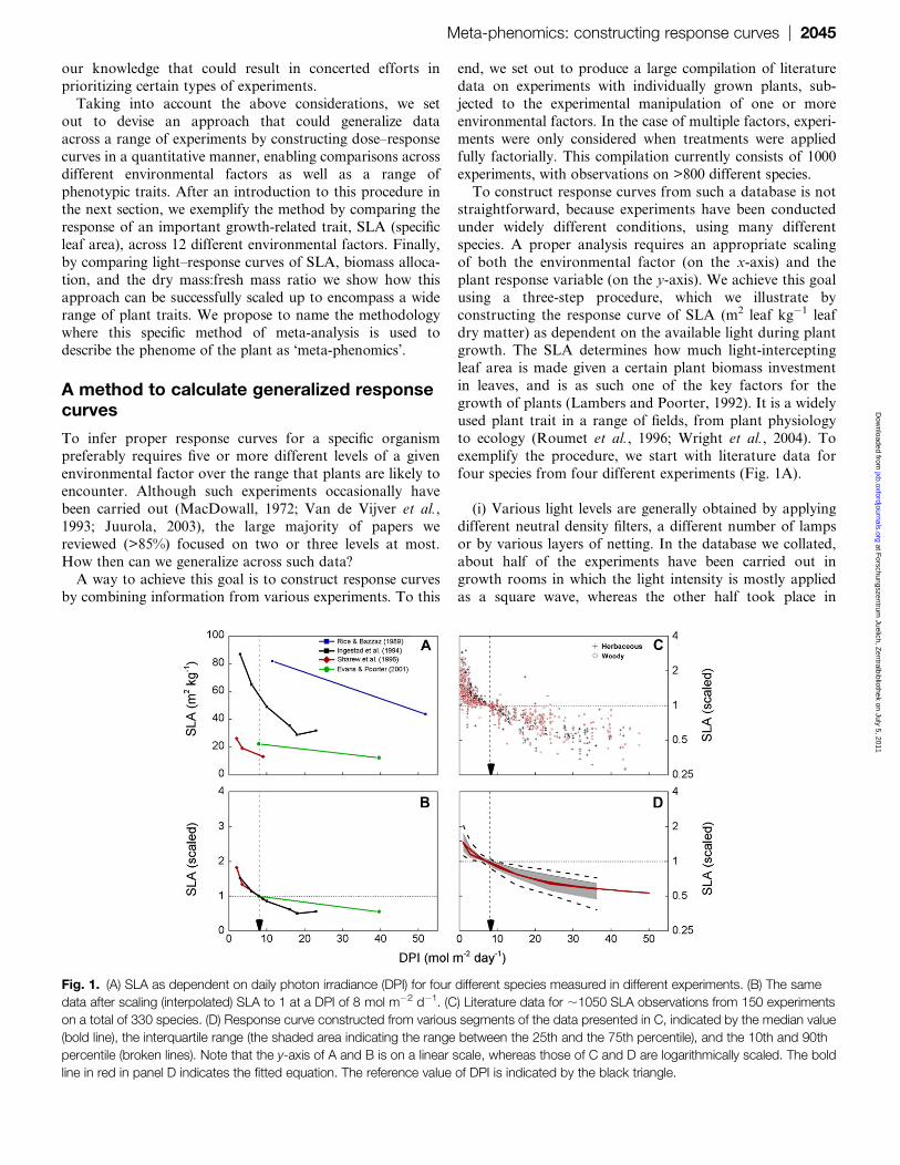
four species from four different experiments (Fig. 1A).

(i) Various light levels are generally obtained by applying

different neutral density filters, a different number of lamps

or by various layers of netting. In the database we collated,

about half of the experiments have been carried out in

growth rooms in which the light intensity is mostly applied

as a square wave, whereas the other half took place in

Fig. 1. (A) SLA as dependent on daily photon irradiance (DPI) for four different species measured in different experiments. (B) The same

data after scaling (interpolated) SLA to 1 at a DPI of 8 mol m�2 d�1. (C) Literature data for ;1050 SLA observations from 150 experiments

on a total of 330 species. (D) Response curve constructed from various segments of the data presented in C, indicated by the median value

(bold line), the interquartile range (the shaded area indicating the range between the 25th and the 75th percentile), and the 10th and 90th

percentile (broken lines). Note that the y-axis of A and B is on a linear scale, whereas those of C and D are logarithmically scaled. The bold

line in red in panel D indicates the fitted equation. The reference value of DPI is indicated by the black triangle.

Meta-phenomics: constructing response curves | 2045 at F



Dow

nloaded from


glasshouses or outdoor in which light varies greatly over the

day. Is there a way to scale light availability in a manner that

enables the combination of data from both types of growth

environments? A suitable solution is to consider the daily

amount of photosynthetic irradiance (DPI), which is the

integrated value of light intensity over the day, because it

correlates much better with, for example, leaf morphology

(Chabot et al., 1979) and plant growth rate (Poorter and Vander Werf, 1998) than light intensity or photoperiod alone.

(ii) Having chosen the appropriate variable on the x-axis,

the next challenge is to choose the units on the y-axis. Plants

differ inherently in SLA (Poorter et al., 2009), and experi-

ments vary in the DPI applied, which precludes an analysis

of absolute values. We therefore chose to extract relativevalues, by defining for each experiment the SLA found at

a DPI of 8.0 mol m�2 d�1 as the reference value to which all

measurements of an experiment were normalized (Fig. 1B).

This value was chosen because most collated experiments

cover a range of DPIs that includes the value of 8.0. It is not

very common, though, that one of the light treatments is

exactly 8.0 mol m�2 d�1. In this case we linearly interpolated

a reference value for SLA from the two adjacent light levels.If a DPI of 8.0 was outside the range considered for a given

experiment, we excluded those data from further analysis,

with the exception of experiments where the highest or lowest

light levels differed by <10% from the reference value. Thus,

of the four studies shown in Fig. 1A, the data of Rice and

Bazzaz (1989) were excluded from further analysis. For each

of the other experiments, observed SLA values at each DPI

are divided by their calculated reference value. Although thethree remaining experiments were characterized by very

different DPIs and species with inherently different SLAs,

they converge well after this scaling procedure (Fig. 1B).

Note that this analysis allows an evaluation of the form of

the response curve, but does not differentiate between species

with inherently different maximum values. A similar normal-

ization procedure is used by Tardieu and Parent (2010), with

interesting insights into the short-term effect of temperatureon leaf elongation rate.

(iii) The third step is to calculate all SLA values for each

experiment and light level relative to the SLA observed or

calculated at a DPI of 8.0 (Fig. 1C). The scaling procedure

yields normalized values (ratios) rather than absolute values.

By their nature, ratios do not show a normal distribution in

a statistical sense, as values <1 can range from 0 to 1, butvalues >1 may approach infinity. As it is of interest to know

whether a given plant trait varies linearly or non-linearly

with an environmental factor, we log2-transformed the

ratios of plant traits before any statistical analysis, as well

as the relevant axes of graphs that we will use further on.

The light–response curve of SLA as anexample

The full database we collated for SLA as dependent on

irradiance currently consists of 160 experiments, with a total

of >300 species and 1200 average values. Approximately

15% of those data are from experiments that do not include

the reference value of 8.0 mol m�2 d�1. They are therefore

excluded from the analysis, although most of them con-

firmed the trends described here (data not shown). The

remaining data set is remarkably diverse: Helianthus annuus

is the most frequently measured species, yet it represents

only 2% of all observations. The single largest experiment isthat of Poorter (1999) on 15 species and six light intensities,

which represents 7% of the observations. In the subsequent

analyses, we no longer consider the separate experiments,

but rather analyse all data points observed across all

experiments concurrently. The resulting data set reveals

a strong decrease in SLA with increasing DPI (Fig. 1C).

However, there is also considerable variation present in the

response. This variation may be caused by: (i) differentspecies responding distinctly; (ii) different levels of environ-

mental factors other than light for different experiments;

(iii) the plant’s ontogenetic stage at the time of harvest; (iv)

possible errors during data collection and/or calculation by

the original authors; and/or (v) errors or inaccuracies

occurring during our analysis of the literature. In so far as

errors in the SLA measurement involve a linear trans-

formation (e.g. a wrong calibration factor or unit ofexpression) they do not affect the current analysis because

all values are expressed in a relative way. A more serious

problem arises if, for example, data are labelled in the paper

as SLA values (leaf area:leaf mass), whereas in reality

calculations pertain to LMA values (leaf mass:leaf area).

This yields data characterized by a similar numerical range,

but by an inverse relationship. In case of doubt, we

contacted authors to double check. However, especially forolder literature, this is not always possible. As the overall

trend is at first more interesting than possible outliers, we

decided to show the trend of the median and the inter-

quartile range. This was done by categorizing the data

points in seven DPI ranges (0–2, 2–4, 4–8, 8–12, 12–20,

20–30, and >30 mol m�2 d�1) and calculating the median

response, as well as the 25th and 75th percentile for each

DPI range. The xth percentile is that value in a group ofobservations at which x% of the total observations show

a smaller number and 100–x% a higher value. The

advantage of percentiles is that they do not require any

assumptions about the distribution of the underlying data

and that they are relatively strongly buffered against

occasional outliers. The median and the interquartile range

are plotted in Fig. 1D as a bold line and grey area,

respectively, and show the ‘main trend’ across all data.Furthermore, we used this approach to set ‘normal limits’,

by calculating the 10th and the 90th percentile. They are

indicated in Fig. 1D as broken lines. As mentioned before,

observations outside this range are not necessarily abnor-

mal, but rather should be considered by researchers with

greater awareness of possible unintended effects.

An explicit aim of our approach is not only to provide an

overall summary of a wide range of experiments, but also tomake the approach quantitative. This may serve as a bench-

mark for future experiments as it can be analysed whether




Dow

nloaded from


a given species responds more or less strongly compared

with the ‘average’ species. To this end, we carried out

a stepwise regression through all data, starting with

a quadratic polynomial equation. In cases where the

second-order equation was significant, we fitted the data

with the formula

y¼aþb�xc ð1Þ

where y is the log2-transformed scaled dependent variable

(in this case SLA), and x is the environmental factor of

interest. Conversely, in cases where the quadratic term or

the whole equation was non-significant, we tested a linear

equation. In the case of light, the relationship for SLA wasclearly negative and non-linear (P <0.001 for the quadratic

term), with an overall r2 of 0.75 (Table 1). The resulting

trend line is shown in Fig. 1D in red and can be used as an

average approximation of the SLA response of plants

to light intensity. We set the likely range of DPI that

plants experience as lying between 1 mol m�2 d�1 and 50 mol

m�2 d�1, extreme specialists not included. From the fitted

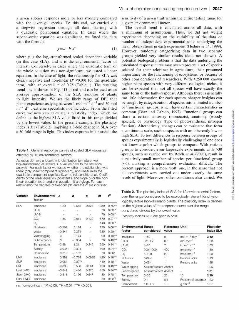
curve we now can calculate a plasticity index, which wedefine as the highest SLA value fitted in this range divided

by the lowest value. In the present example, the plasticity

index is 3.1 (Table 2), implying a 3-fold change in SLA over

a 50-fold range in light. This index captures in a nutshell the

sensitivity of a given trait within the entire testing range for

a given environmental factor.

The overall trend is calculated across all data, with

a minimum of assumptions. Thus, we did not weight

experiments depending on the variability of the data or

number of independent experimental units underlying the

mean observations in each experiment (Hedges et al., 1999).

However, randomly categorizing data in two separategroups yielded very similar results (data not shown). A

potential biological problem is that the data underlying the

calculated response curve may over-represent a set of species

selected for their relevance in agriculture, their presumed

importance for the functioning of ecosystems, or because of

other considerations of researchers. With >250 000 known

higher plant species with very different ecological niches, it

can be expected that not all species will have exactly thesame form of the light–response. Although there is generally

too little information for each species, sharper insights can

be sought by categorization of species into a limited number

of ‘functional’ groups, which have certain characteristics in

common (Dıaz and Cabido, 1997). Functional groups can

share a certain ancestry (monocots), anatomy (woody

species), or physiology (type of photosynthesis, nitrogen

fixation). Alternatively, changes can be evaluated that forma continuous scale, such as species with an inherently low or

high SLA. To test differences in response between groups of

species experimentally is logistically challenging if one does

not know a priori which groups to compare. With various

groups to consider, even large-scale experiments with >30

species, such as carried out by Reich et al. (2003), result in

a relatively small number of species per functional group

(<6), making a comprehensive evaluation difficult. Thepresent approach is a more ‘soft’ one, in the sense that not

all experiments were carried out under exactly the same

levels of light. Moreover, other conditions also varied. We

Table 1. General response curves of scaled SLA values as

affected by 12 environmental factors

As ratios do have a logarithmic distribution by nature, welog2-transformed all scaled SLA values prior to the statisticalanalysis. For each factor we tested whether the relationship waslinear (only linear component significant), non-linear (also thequadratic component significant), or no relationship at all. Coeffi-cients of the linear equation (constant a and slope b) or the non-linear equation (a, b, and c in equation 1) are given. For eachrelationship the degrees of freedom (df) and the r2 are indicated.

Variable Environmentalfactor

a b c df r2

SLA Irradiance 1.20 –0.642 0.324 1050 0.75***

R:FR – – – 70 0.00ns

UV-B – – – 70 0.00ns

CO2 1.86 –0.811 0.139 670 0.27***

O3 – – – 140 0.00ns

Nutrients –0.194 0.184 – 720 0.06***

Water –0.344 0.334 – 330 0.20***

Waterlogging 0 –0.174 – 90 0.19***

Submergence 0 –0.904 – 70 0.40***

Temperature –2.56 1.21 0.249 390 0.44***

Salinity 0.0351 –0.304 – 190 0.24***

Compaction 0.216 –0.162 – 70 0.06*

LMF Irradiance 0.961 –0.794 0.0920 420 0.16***

SMF Irradiance 0.064 –0.0074 – 410 0.10***

RMF Irradiance –0.889 0.508 0.261 420 0.48***

Leaf DMC Irradiance –0.841 0.486 0.275 150 0.84***

Stem DMC Irradiance –0.511 0.156 0.547 80 0.78***

Root DMC Irradiance – – – 80 0.00ns

ns, non-significant; *P <0.05; **P <0.01; ***P <0.001.

Table 2. The plasticity index of SLA for 12 environmental factors,

over the range considered to be ecologically relevant for physio-

logically active (non-dormant) plants. The plasticity index is defined

as the highest value of the response curve over the range

considered divided by the lowest value

Plasticity indices >1.5 are given in bold.

Environmentalfactor

Rangeconsidered

Referencevalue

Unit Plasticityindex SLA

Irradiance 1–50 8 mol m�2 day�1 3.12

R:FR 0.2–1.2 0.9 mol mol�1 1.00

UV-B 1–20 7 kJ m�2 d�1 1.00

CO2 200–1200 400 lmol mol�1 1.39

O3 5–100 20 nmol mol�1 1.00

Nutrients 0.02–1 1 Relative units 1.13

Water 0.05–1 1 Relative units 1.25

Waterlogging Absent/present Absent – 1.06

Submergence Absent/present Absent – 1.81

Temperature 5–35 20 �C 2.19

Salinity 0–1 0.1 Fraction of seawater 1.23

Compaction 1.0–1.6 1.2 g cm�3 1.07




Dow

nloaded from


therefore cannot exclude the possibility that in some experi-

ments another factor, for example a suboptimal nutrient

supply, interacted with the response of plants to light. In the

case of factorial combinations of treatments, we therefore

focused on that level of the environmental factors outside

our direct interest that yielded plants with the highest

biomass. In the case of unifactorial experiments, we simply

have to rely on the expertise of the researchers in choosingthe appropriate growth conditions. Variability in the

environmental factors that are not directly of interest is not

only a nuisance: the wide variety of experiments compiled

here also offers an advantage, as it implies that the observed

trends are probably more generally valid than the results of

one large experiment which was carried out under one

specific combination of environmental factors. However, to

exclude fully the possibility of confounding effects, anyresult from this analysis should be independently tested in

a directed experiment.

Analysing response curves for contrastingsubgroups

As an extension to the above analysis we classified species in

a number of categories, as listed in the ‘species trait’ box of

Fig. 2. Furthermore, we characterized general experimental

conditions, as listed in the conditions box of the same

figure. The third classification was the most challenging, as

we categorized species in accordance with their ecologicalniche. For each environmental factor considered, species

were classified on a three-point scale, discriminating be-

tween species generally found in shaded conditions, a group

of species found mainly in light-exposed habitats, and an

intermediate group. Separate response curves were con-

structed for each subgroup of species, and the plasticity

index calculated as the most concise index of variation in

the response curve.

Particular cultivation conditions seem to matter, as the

plasticity index is higher for plants grown in growth

cabinets than for those growing outdoors, and plants grown

in hydroponics respond more strongly than those in a solid

rooting medium (Table 3). At the same time, woody speciesfrom both the Gymnosperm and Angiosperm clades

responded less strongly than herbaceous monocots and

dicots. In our data set, these factors are strongly con-

founded: 90% of the data for woody species are from open

shade houses constructed in experimental gardens, whereas

85% of the data from growth chambers are for herbaceous

plants, often (>50%) grown in hydroponics. It is therefore

as yet impossible to separate accurately the importance oflife form and growth environment. However, documenta-

tion of this strong confounding between life form and

growth conditions may help in data interpretation as well as

decisions concerning future experimentation.

Three other biological classifications that we made

yielded differences in plasticity, with little confounding of

growth environment. Deciduous woody species had a some-

what greater plasticity than evergreen woody species,although the difference was relatively small and not

significant (Table 3). A second classification pertains to the

debate as to whether species with their ecological niche in

shady habitats show less plasticity for SLA than those

characteristic of sun-exposed environments (see Portsmuth

and Niinemets, 2007 for an extended discussion). Taken

over all experiments and plant species, we found this to be

statistically true, as there was a significant interactionbetween light class and tolerance group. However, the

Fig. 2. The characterization of experiments, as carried out in the current meta-phenomics approach. Plant species are classified

according to the species box by a number of general characteristics. General experimental conditions are given in the experimental box.

The ecological niche of species is estimated by a three-stage scale for the relevant environmental factors. The last box shows the 12

environmental factors considered in this paper. In the case of nutrients, experiments are considered that apply limitations by nitrogen (N),

phosphorus (P), or nutrients in general (G).




Dow

nloaded from


differences seem not to be very large (Fig. 3A). The

difference became stronger when experiments carried out in

growth chambers were excluded (56% difference; data not

shown). A last comparison we made relates to a continuous

trait rather than a categorical one. During the normaliza-

tion procedure all observed SLA values were scaled to

the reference value calculated at a light intensity of 8 molm�2 d�1. Although we statistically corrected for what is

most probably innate variation between species to compare

curves in a standardized way, we can still use the in-

formation to discriminate between inherently low SLA and

high SLA species. Given that there is such a large difference

in SLA between herbaceous and woody species, an un-

conditional comparison would yield a result discussed above

already. Therefore, we contrasted the plants with the 35%lowest and 35% highest SLA values within each life form.

Differences were more pronounced in this case, with high

SLA species from both life forms responding more strongly

than low SLA species (Fig. 3B; P <0.001 in both cases).

The response of SLA to 12 environmentalfactors

The above analysis provides a condensed summary of the

response of SLA to light over a wide range of experiments.

All data were systematically expressed in the same units of

irradiance as well as the same units describing leafmorphology. Although highly informative in itself, light

forms only one axis in a multidimensional space of

environmental factors. Far more insight could be achieved

if we were able to have similar information for the other

environmental dimensions as well. In a recent review,

Poorter et al. (2009) considered the response of LMA to

a wide range of environmental factors. Among these are the

‘general’ factors that received the greatest attention in thescientific field up to now: light, CO2, nutrients, temperature,

and water limitation. However, also more specific stresses,

such as UV-B, ozone, waterlogging, submergence, salinity,

and soil compaction can be highly relevant for plant

functioning and are included in the analysis. We did not

include abiotic stresses such as trampling, wind, SO2, and

NOx, not because they are irrelevant, but simply because

too little information is available to allow for a propergeneralization. As for light, we focus on plants that are

generally grown for the longest period of their active

growing time under contrasting environmental conditions,

without experimentally designed switches between environ-

ments. The only exception is complete submergence, which

is a stress factor that most land plants can endure for only

Fig. 3. SLA response to daily photon irradiance as dependent on

various subgroups. (A) The median response of plant species

characteristic of shaded habitats (blue line), sun-exposed habitats

(red line), or from intermediate environments (green line). (B) The

median response of species with a relatively high (red line) or low

(blue line) SLA at the reference irradiance of 8 mol m�2 d�1,

analysed separately for woody (broken line) and herbaceous

species (continuous line). The reference value for the different

environmental factors is indicated by black arrows.

Table 3. Plasticity indices for specific leaf area (SLA) of different

subgroups over the daily photon irradiance (DPI) range of

1–50 mol m�2 d�1

A non-linear equation was fitted to various subgroups of observa-tions. For some groups this included some extrapolation of the data,but ranking of differences remained the same when a smallertrajectory was considered. The plasticity index is defined as thehighest value of the response curve over the range considereddivided by the lowest value. The last column indicates thesignificance of differences in plasticity between subgroups. To thisend, we tested with orthogonal polynomials for a significant sub-group3light class interaction, considering only the linear component.This indicates whether there are differences in plasticity betweensubgroups, which linearly increase or decrease over the whole lightrange considered, neglecting higher order fluctuations. In the case ofthe ecological classifications this implies an increasing or decreasingplasticity across the species groups

Subgroup Plasticityindex SLA

df P, betweensubgroups

Growth environment Cabinets 3.52 290 ***

Glasshouses 3.07 210

Experimental garden 2.73 330

Root substrate Hydroponics 4.09 140 ***

Soil 2.90 660

Phylogenetic/life form Herbaceous dicots 3.90 280 ***

Herbaceous monocots 3.67 80

Woody dicots 2.87 630

Woody gymnosperms 2.74 30

Leaf habit Woody dicots deciduous 2.90 260 ns

Woody dicots evergreen 2.59 400

Shade tolerance Low 3.45 480 ***

Intermediate 2.76 370

High 2.71 150

ns, non-significant; ***P <0.001.




Dow

nloaded from


a limited amount of time. A detailed description of the

restrictions used for this review is given in Appendix 1.

Here we extend the analysis of Poorter et al. (2009), with

;20% more experiments, and present all leaf area:biomass

ratios as SLAs. Although SLA and LMA carry the same

information, they are inversely related, which can make

analysis of linear and non-linear responses difficult. More-

over, for a large group in the scientific community, SLA isa more appropriate parameter to use, as it scales in

principle linearly with the relative growth rate of plants

(Evans, 1972). In total, we considered SLA responses to 12

environmental factors. For 10 factors, an objectively

measurable reference value could be chosen. A critical

criterion for the choice of the reference value is that it falls

in the range of values usually measured. In principle, the

actual level of choice does not affect the final result.Reference values are listed in Table 2 and indicated by

black triangles in Fig. 4. The main problem we faced was

choosing a reference level for nutrient and drought stress.

There are many ways in which nutrient stresses can be

applied (Ingestad et al., 1982; Van de Vijver et al., 1993),

with a wide range of results possible, which depend on the

details of the experimental design on the one hand and the

size as well as the growth rate of the plants—and thereforethe demand for nutrients—on the other. In the case of

drought stress, the experimental designs vary as greatly as

for nutrients (Fernandez and Reynolds, 2000; Granier et al.,

2006). The only possible way to scale the severity of these

stresses is by expressing them relative to the total biomass

gained by control plants. This is not ideal, as the control

plants may have suffered from stress in some experiments

and not in others, but it is possibly as close as one can get ingeneralizing the severity of a stress over such a variety of

experiments. For the factors waterlogging and complete

submergence, we only considered two levels: either fully

waterlogged or submerged, or well-watered controls,

neglecting a more fuzzy intermediate level such as ‘70%

submerged’. A level of 100% waterlogging or submergence

is still objectively definable.

The results of the analysis are shown in Fig. 4A–L. Thenumber of data we have been able to find and that underlie

these response curves varies greatly between factors, with

the least information on R:FR, UV-B, and soil compaction.

These are at the same time the factors that turn out to have

little impact on SLA, which may actually be the prime

reason why they are not reported as often. Another

environmental factor, for which little information is present,

is complete submergence. In this case, the increase in SLA islarge, and has been thought to be one of the important

traits determining the ability to survive in such an environ-

ment (Mommer et al., 2006). For a more quantitative

analysis, we fitted for each factor general response curves

over all data. Taking then into account the biologically

relevant range for each environmental factor (Table 3),

plasticity indices were calculated over these ranges. Plastic-

ity for SLA varied widely, being highest for light, sub-mergence, and temperature, and only modest for CO2,

nutrients, drought, and salinity. An extended discussion of

the underlying mechanisms is outside the scope of this

paper, and can be found in Poorter et al. (2009).

Variability, as judged from the interquartile range, is also

an important issue in judging these response curves. As

a consequence of the normalization procedure, variability is

smallest close to the reference values, indicated by the black

triangles. The factors with the strongest variability are those

for which the response is generally strong anyway, whichmay be caused by species specialization. We included two

clear examples of this phenomenon in Fig. 4. The median

response to CO2 is stronger than average for C3 species

(Fig. 4D). The response of C4 species is in stark contrast; it

does not respond to elevated CO2 up to a range of 800 lmol

mol�1 and—surprisingly—even increases at higher concen-

trations. Although the number of data on C4 plants at high

CO2 levels is low, the difference is significantly differentfrom unity. The other example is that of temperature (Fig.

4J), highlighting that tropical species show a much higher

plasticity in SLA for this factor than plants from temperate

climates.

The response curves of different traits canbe compared

The above analysis shows how the response of one trait

can be analysed over a range of environmental factors.

However, the approach can be fruitfully extended to other

variables. As an example, we show here the response ofbiomass allocation and the dry matter content (DMC) with

respect to growth irradiance. The allocation of biomass over

the various plant organs has received attention for a long

time, in both a physiological and ecological context.

Brouwer (1962) coined the appealing term ‘functional

equilibrium’ for the way biomass was allocated to shoots

and roots under various environmental conditions, and

Tilman (1988) used it as cornerstone for his theory on theecological success of species. Following the same approach

as for SLA, we compiled ;440 observations on the fractions

of biomass invested in leaves, stems, and roots (termed

LMF, SMF, and RMF, respectively). Response curves are

shown in Fig. 5, at the same scale as was used for the SLA

data. As can be seen from this graph, the changes are very

modest. There is some shift towards a decreased allocation

to roots and an increased allocation to leaves at lower lightlevels, but only when the light level is very low (<3 mol m�2

d�1) does the shift in LMF become more apparent.

Although this trend can be considered to agree well with

a ‘functional equilibrium’ paradigm, the changes are overall

marginal, with a plasticity index for LMF of 1.26, which is

small compared with the 3-fold change in SLA. We therefore

conclude that the differences in SLA are more important

than the variation in LMF in understanding the variation inrelative growth rate with light. A second point that is nicely

illustrated by these data is the care that has to be taken in

their interpretation. Presented on the same relative scale,

LMF seems to be less plastic than RMF (plasticity index ¼1.91). However, compared with leaves, roots generally




Dow

nloaded from


comprise a smaller fraction of biomass of young trees and

herbaceous plants. Thus, if a plant allocates 1 g less to leaves

but rather invests this in roots, the relative decrease in LMF

will be smaller than the relative increase in RMF.

Another trait that has received little attention so far is the

DMC (dry mass:fresh mass) of various organs. There are

strong and inherent differences in DMC for ecologically

different species. In fact, in the ecological literature it has

Fig. 4. (A–L) The response of specific leaf area (SLA) to 12 environmental factors. The bold line indicates the median value, and the

shaded area the interquartile range. The number of observations on which this graph is based is listed in Table 1. The reference value for

the various environmental factors is indicated by black arrows. D also shows the median response of C3 and C4 species separately and J

shows the median response of species characteristic of environments with different temperatures during the growing period.




Dow

nloaded from


been suggested that leaf DMC would be a better parameter

to determine a plant’s ecological niche than SLA (Wilson

et al., 1999). However, also for physiological research, the

DMC of the various organs is an important variable to

consider, not least because various publications use various

ways to scale rates of physiological processes or chemical

amounts across treatments or species. Thus, some scientists

prefer to express rates of processes or amounts of com-pounds per unit area, especially in photosynthesis-related

research (Hurry et al., 1995; Pons and De Jong, 2004),

others generally use dry masses (De Groot et al., 2003), and

still others report their results routinely on a fresh mass

basis (Smith and Stitt, 2007; Usadel et al., 2008). It follows

that if we do not know the relationships between these three

parameters, it is hard to make a useful integration across

experiments. Therefore, we looked at how irradiance affects

the DMC of the various organs.

In strong contrast to SLA and biomass allocation, there

are very few reports on the DMC of organs as dependent on

the environment, notwithstanding the fact that fresh and

dry masses are routinely measured in many laboratories.Therefore, the majority of the data on which Fig. 6 are

based are not from the literature, but are unpublished data

kindly shared by colleagues mentioned in the Acknowledge-

ments section. Leaf DMC turned out to be surprisingly

strongly affected by light, with an almost linear increase in

DMC when light increases. The plasticity index for this trait

Fig. 5. The response of the allocation of biomass to (A) leaves

(LMF), (B) stems (SMF), and (C) roots (RMF) to irradiance. The bold

line indicates the median value and the shaded area the interquartile

range. The number of observations on which this graph is based is

listed in Table 1. The reference value of the DPI is indicated by black

arrows.

Fig. 6. Response curves of the dry matter content (DMC) of (A)

leaves, (B) stems, and (C) roots to irradiance. The number of

observations on which this graph is based is listed in Table 1. The

reference value of the DPI is indicated by black arrows.




Dow

nloaded from


is 1.92, which is less than that for SLA, but still consider-

able. The same holds for the DMC of the stems (2.25), but,

very surprisingly, the DMC of the roots is hardly affected

by the light environment. In general, the underlying basis

for differences in DMC can be 3-fold. First, there can be

a difference in the concentration of cell wall compounds,

because of higher allocation to cell walls, a shift from water-

rich epidermal tissue to other tissues, such as sclerenchy-matic cells, or because of changes between leaf veins and

interveinal areas (cf. Van Arendonk and Poorter, 1997;

Niinemets, 1999; Walter and Schurr, 1999; Niinemets and

Sack, 2006). Secondly, the cell size can be affected, with

smaller cells and (much) smaller vacuoles, which will also

increase the relative fraction of dry matter in cell walls

(Niinemets and Sack, 2006). Thirdly, the content can be

affected by accumulation of large quantities of, for example,starch. Although starch concentrations are higher at high

light, these differences are modest compared with those of

plants grown at elevated CO2 (Roumet et al., 1999) or in

cold conditions (Venema et al., 1999). Currently, we do not

have a satisfactory understanding of the quantitative

importance of each of these factors.

Conclusions and outlook

The procedures presented here build on a large database of

phenotypic observations and provide a quantitative methodto construct response curves. Using SLA as an example of

an important phenotypic trait, we were able to show that

the use of this methodology enabled: (i) the construction of

quantitative relationships with 12 environmental factors; (ii)

the estimation of variability around median trends; (iii) the

characteristic response of certain pre-defined experimental

subgroups; and (iv) the definition of a plasticity index over

the full range of an environmental factor. The quantitativerelationships found can form a reference for results of

future experiments, and provide the framework of prior

knowledge as required, for example, in Bayesian statistics

(McCarthy, 2007).

We have shown that this meta-analytical approach can be

fruitfully extended to other phenotypic data. We will target

a larger number of physiological, morphological, chemical,

and anatomical plant traits, such as photosynthetic capac-ity, biomass allocation, and nitrogen content. In future

analysis, another focal point will be the interaction between

different variables. We refer to this approach as ‘meta-

phenomics’, which provides us with a more systematic and

formal way to structure information on the response of

plants to their environment. This will be advantageous, in

understanding both the constraints to plant productivity by

limiting factors and the response of plants to global change.

Supplementary data

Supplementary data are available at JXB online.

Supplementary appendix 1. List of papers used for the

analysis of the effect of 12 environmental factors on SLA.

Supplementary appendix 2. List of papers used for the

analysis of the effect of irradiance on allocation and dry

matter content.

Acknowledgements

We thank Ismael Aranda, Owen Atkin, Corine de Groot,

Yulong Feng, Keith Funnell, Yaskara Hayashida, Vaughan

Hurry, Maarit Maenpaa, Kerstin Nagel, Leo Marcelis, Thijs

Pons, Peter Reich, Dina Rhonzina, Francesco Ripullone,

Catherine Roumet, Peter Ryser, Dylan Schwilk, Susanne

Tittman, Jan Henk Venema, and Rafael Villar, for gener-

ously providing (partly) unpublished results for this analysis.

Lea Hallik, Harry Olde Venterink, and Hans Schepers as wellas the reviewers provided insightful comments on a previous

version of the manuscript. HP acknowledges support from

the Estonian University of Life Sciences and the Estonian

Ministry of Education and Science (grant SF1090065s07)

for his stay during the writing of this manuscript.

Appendix 1. Inclusion criteria for the meta-analyses

We believe that this approach could be used to generalize acrossa wide variety of experiments and conditions. Accordingly, weadopted by default an inclusive approach in considering previouslypublished work. However, we wish to list explicitly the fewdecisional criteria that we applied consistently to define a finalselection of data.

(i) We only considered plants that were subjected to some formof controlled experimental treatment involving the directmanipulation of environmental variables, and thus excludedplants growing in the field for which correlations were madewith measured environmental variables a posteriori. How-ever, these observations can form interesting comparisonswith our results (Ogaya and Penuelas, 2007).

(ii) We only considered plants grown in pots, hydroponics, orother types of containers, in the absence of competition withneighbouring plants. Thus we excluded plants growing inintra- or interspecific competition for light (such as inartificial vegetations), or nutrients (such as in experimentalgardens in naturally occurring soil).

(iii) We considered three plant organs: leaves, stems, and roots. Incases where concentrations or biomass allocation werepresented on a shoot basis, these observations were disre-garded. An exception was made for rosette plants, where thecaudex would form a small proportion of the shoot anyway.

(iv) Plants in the generative phase may show a different responseto those in the vegetative phase, especially at the whole plantlevel, and for this review we focus on the vegetative phaseonly.

(v) In the case of an experiment with a factorial combination ofenvironmental factors, we choose the response of plants tothe factor of interest at the level of the other environmentalconditions that were least limiting.

References

Arp WJ. 1991. Effects of source–sink relations on photosynthetic

acclimation to elevated CO2. Plant, Cell and Environment 14,

869–875.




Dow

nloaded from

Supplementary data

Supplementary appendix 2.

Supplementary appendix 2.


Bezemer PD, Netelenbos JC, Mulder C, Theune JA,

Stamhuis IH, Straus JP. 1982. Determining reference (normal) limits

in medicine: an application. Statistics in Medicine 2, 191–198.

Brouwer R. 1962. Distribution of dry matter in the plant. Netherlands

Journal of Agricultural Sciences 10, 399–408.

Chabot BF, Jurik TW, Chabot JF. 1979. Influence of instantaneous

and integrated light-flux density on leaf anatomy and photosynthesis.

American Journal of Botany 66, 940–945.

De Groot CC, Marcelis LFM, Van den Boogaard R, Kaiser WM,

Lambers H. 2003. Interaction of nitrogen and phosphorus nutrition in

determining growth. Plant and Soil 248, 257–268.

De Groot CC, Marcelis LFM, Van den Boogaard R, Lambers H.

2002. Interactive effects of nitrogen and irradiance on growth and

partitioning of dry mass and nitrogen in young tomato plants.

Functional Plant Biology 29, 1319–1328.

Dıaz S, Cabido M. 1997. Plant functional types and ecosystem

function in relation to global change. Journal of Vegetation Science 8,

463–474.

Evans GC. 1972. The quantitative analysis of plant growth. Oxford:

Blackwell.

Evans LT, Wardlaw IF, King RW. 1985. Plants and environment:

two decades of research at the Canberra phytotron. Botanical Review

51, 203–272.

Farquhar GD, Von Caemmerer S, Berry JA. 2001. Models of

photosynthesis. Plant Physiology 125, 42–45.

Fernandez RJ, Reynolds JF. 2000. Potential growth and drought

tolerance of eight desert grasses: lack of a trade-off? Oecologia 123,

90–98.

Granier C, Aguirrezabal L, Chenu K, et al. 2006. PHENOPSIS, an

automated platform for reproducible phenotyping of plant responses

to soil water deficit in Arabidopsis thaliana permitted the identification

of an accession with low sensitivity to soil water deficit. New

Phytologist 169, 623–635.

Hanson HC. 1917. Leaf-structure as related to environment.

American Journal of Botany 4, 533–560.

Hedges LV, Gurevitch J, Curtis PS. 1999. The meta-analysis of

response ratios in experimental ecology. Ecology 80, 1150–1156.

Hedges LV, Olkin I. 1985. Statistical methods for meta-analysis.

Orlando: Academic Press.

Hikosaka K, Osone Y. 2009. A paradox of leaf-trait convergence:

why is leaf nitrogen concentration higher in species with

higher photosynthetic capacity? Journal of Plant Research 122,

245–251.

Hurry VM, Strand A, Tobiaeson M, Gardestrom P, Oquist G.

1995. Cold hardening of spring and winter wheat and rape results in

differential effects on growth, carbon metabolism, and carbohydrate

content. Plant Physiology 109, 697–706.

Ingestad T. 1982. Relative addition rate and external concentration;

driving variables used in plant nutrition research. Plant, Cell and

Environment 5, 443–453.

Juurola E. 2003. Biochemical acclimation patterns of Betula pendula

and Pinus sylvestris seedlings to elevated carbon dioxide

concentrations. Tree Physiology 23, 85–95.

Kreusler U, Prehn A, Hornberger R. 1879. Beobachtungen uber

das Wachstum der Maispflanze (Bericht uber die Versuche vom Jahre

1878). Landwirtschaftliche Jahrbucher 8, 617–622.

Lambers H, Poorter H. 1992. Inherent variation in growth rate

between higher plants: a search for physiological causes and ecological

consequences. Advances in Ecological Research 23, 187–261.

Macdowall FDH. 1972. Growth kinetics of Marquis wheat. I. Light

dependence. Canadian Journal of Botany 50, 89–99.

McCarthy MA. 2007. Bayesian statistics for ecology. Cambridge:

Cambridge University Press.

Mitscherlich E. 1909. Das Gesetz des Minimum, das Gesetz des

Abnahmenden Bodenertrages. Landwirtschaftliches Jahrbuch 38,

537–552.

Mommer L, Lenssen JPM, Huber H, Visser EJW, de Kroon H.

2006. Ecophysiological determinants of plant performance under

flooding: a comparative study among seven plant families. Journal of

Ecology 94, 1117–1129.

Morgan PB, Ainsworth EA, Long SP. 2003. How does elevated

ozone impact soybean? A meta-analysis of photosynthesis, growth

and yield. Plant, Cell and Environment 26, 1317–1328.

Niinemets U. 1999. Research review. Components of leaf dry mass

per area—thickness and density—alter leaf photosynthetic capacity in

reverse directions in woody plants. New Phytologist 144, 35–47.

Niinemets U Sack L. 2006. Structural determinants of leaf light-

harvesting capacity and photosynthetic potentials. In: Esser K, Luttge

UE, Beyschlag W, Murata J, eds. Progress in botany, vol. 67. Berlin:

Springer Verlag, 385–419.

Ogaya R, Penuelas J. 2007. Leaf mass per area ratio in Quercus ilex

leaves under a wide range of climatic conditions. The importance of

low temperatures. Acta Oecologia 31, 168–173.

Osenberg CW, Sarnelle O, Cooper SD. 1997. Effect size in

ecological experiments: the application of biological models in meta-

analysis. American Naturalist 150, 798–812.

Pons TL, De Jong-van Berkel YEM. 2004. Species-specific

variation in the importance of the spectral quality gradient in canopies

as a signal for photosynthetic resource partitioning. Annals of Botany

94, 725–732.

Portsmuth A, Niinemets U. 2007. Structural and physiological plasticity

in response to light and nutrients in five temperate deciduous woody

species of contrasting shade tolerance. Functional Ecology 21, 61–77.

Poorter H. 1993. Interspecific variation in the growth response of plants

to an elevated ambient CO2 concentration. Vegetatio 104/105, 77–97.

Poorter H, Navas ML. 2003. Plant growth and competition at

elevated CO2: on winners, losers and functional groups. New


Poorter H, Niinemets U, Poorter L, Wright IJ, Villar R. 2009.

Causes and consequences of variation in leaf mass per area (LMA):

a meta-analysis. New Phytologist 182, 565–588.

Poorter H, van der Werf A. 1998. Is inherent variation in RGR

determined by LAR at low irradiance and by NAR at high irradiance? A

review of herbaceous species. In: Lambers H, Poorter H, Van Vuuren

MMI, eds. Inherent variation in plant growth. Physiological

mechanisms and ecological consequences. Leiden, The Netherlands:

Backhuys Publishers, 309–336.




Dow

nloaded from


Poorter L. 1999. Growth responses of 15 rain-forest tree species to

a light gradient: the relative importance of morphological and

physiological traits. Functional Ecology 13, 396–410.

Reich PB, Buschena C, Tjoelker MG, Wrage K, Knops J,

Tilman D, Machado JL. 2003. Variation in growth rate and

ecophysiology among 34 grassland and savanna species under

contrasting N supply: a test of functional group differences. New


Rice SA, Bazzaz FA. 1989. Quantification of plasticity of plant traits in

response to light intensity: comparing phenotypes at a common

weight. Oecologia 78, 502–507.

Roumet C, Bel MP, Sonie L, Jardon F, Roy J. 1996. Growth

response of grasses to elevated CO2: a physiological plurispecific

analysis. New Phytologist 133, 595–603.

Roumet C, Laurent G, Roy J. 1999. Leaf structure and chemical

composition as affected by elevated CO2: genotypic responses of two

perennial grasses. New Phytologist 143, 73–81.

Smith A, Stitt M. 2007. Coordination of carbon supply and plant

growth. Plant, Cell and Environment 30, 1126–1149.

Tardieu F, Parent B. 2010. Modelling the effects of genes and QTLs:

on the plant sensitivity to environmental conditions. Journal of

Experimental Botany, in press.

Tilman D. 1988. Plant strategies and the dynamics and structure of

plant communities. Princeton, NJ: Princeton University Press.

Usadel B, Gibon Y, Blasing OE, Poree F, Hohne M, Gunter M,

Trethewey R, Kamlage B, Poorter H, Stitt M. 2008. Multilevel

genomics analysis of the response of transcripts, enzyme activities

and metabolites in Arabidopsis rosettes to a progressive decrease of

the temperature in the non-freezing range. Plant, Cell and Environment

31, 518–547.

Van Arendonk JJCM, Poorter H. 1994. The chemical composition

and anatomical structure of leaves of grass species differing in relative

growth rate. Plant, Cell and Environment 17, 963–970.

Van de Vijver CADM, Boot RGA, Poorter H, Lambers H. 1993.

Phenotypic plasticity in response to nitrate supply of an inherently fast-

growing species from a fertile habitat and an inherently slow-growing

species from an infertile habitat. Oecologia 96, 548–554.

Venema JH, Posthumus F, De Vries M, Van Hasselt PR. 1999.

Differential response of domestic and wild Lycopersicon species to

chilling under low light: growth, carbohydrate content,

photosynthesis and the xanthophyll cycle. Physiologia Plantarum

105, 81–88.

Walter A, Schurr U. 1999. The modular character of growth in

Nicotiana tabacum plants under steady state nutrition. Journal of

Experimental Botany 50, 1169–1177.

Went FW. 1957. The experimental control of plant growth. New York:

The Ronald Press Company.

Wilson PJ, Thompson K, Hodgson JG. 1999. Specific leaf area and

leaf dry matter content as alternative predictors of plant strategies.

New Phytologist 143, 155–162.

Wright IJ, Reich PB, Westoby M, et al. 2004. The leaf economics

spectrum worldwide. Nature 428, 821–827.




Dow

nloaded from


a method to construct dose–response curves for a wide

Documents