a method using epoch-era analysis to identify...

1

A Method Using Epoch-Era Analysis to Identify Valuable Changeability in System Design

Matthew E. Fitzgerald Massachusetts Institute of Technology

77 Mass Ave, E38-550 Cambridge, MA 02139

[email protected]

Adam M. Ross Massachusetts Institute of Technology


[email protected]

Donna H. Rhodes Massachusetts Institute of Technology


[email protected]

Abstract

Changeability is a means of creating value robustness in engineering systems that is currently less understood and correspondingly less utilized than more traditional passive robustness. This paper presents a new approach for investigating system changeability using Epoch-Era Analysis, with an emphasis on tradespace exploration using an illustrative case study. Epoch-Era Analysis is an approach for describing systems over time as existing in a series of static contexts (epochs) that change stochastically. A five-step method is used to generate an intuitive and accessible set of data and graphs describing the abstract concept of changeability, which is difficult to grasp due to its intrinsically time-dependent nature. Ideas for future changeability metrics are discussed.

Motivation and Previous Research

Changeability in Engineering. Changeability is an abstract design concept that is experiencing increased interest as engineering systems grow, both in cost commitment and system lifetime. The perceived potential performance advantages of changeable systems, the difficulty of designing a system fully robust to changes over decades, and the increased cost of failure are driving the increased level of interest in changeability and related “ilities”. However, imprecision in the usage of the word “changeability” and the other “ilities” has created a barrier that must be surmounted to properly understand the concept. The basic understanding is simple and universal: changeability is nothing more than the ability of a system to change. However, the meaning of that phrase is subject to a wide range of interpretations, largely based on the system application it is being used to describe. For example, a term with many similarities to changeability is flexibility; indeed, the words are used interchangeably quite often in the literature. Saleh et al. (2009) performed a survey of the use of the word “flexibility” in the literature for different fields, mainly managerial, manufacturing, and engineering design, while cataloguing the different meanings of the usage. Focusing here on the meaning for engineering systems, Saleh finds two distinct uses: one for flexibility in the design process and another for flexibility in the design itself. Even these subcategories of flexibility have been used differently, with design process flexibility being applied to both customers (flexibility in requirements

9th Conference on Systems Engineering Research Los Angeles, CA, April 2011 Pre-print

2

specified) and designers (flexibility in constraints imposed). In-design flexibility is similarly split amongst various definitions, although most relate quite directly to the ability of the system to perform different functions.

Fricke and Schulz (2005) published a paper summarizing unifying principles behind designing for changeability (DfC) in engineering. In addition to covering the motivation for changeability in the modern technological environment, they identified four key dimensions of changeability: robustness, flexibility, agility, and adaptability. All four of these dimensions would fall under Saleh’s in design flexibility subcategory, as they are used to characterize the changeability of designs and not of the designing process. According to DfC, robustness is the ability of a system to withstand environmental changes while flexibility is the ability to alter the system in response to those changes. The key difference between the two is the passive nature of robustness versus the active nature of flexibility, two different approaches to delivering value over time. Adaptability fits in between the two, as it is defined as the ability of a system to change itself in response to the environment; depending on the frame of reference this can be viewed as passive (frame is around the system, no external input) or active (frame is within the system, the environment is an input). Agility is defined as the ability to change in a short time frame, and can be applied to both internal and external changes.

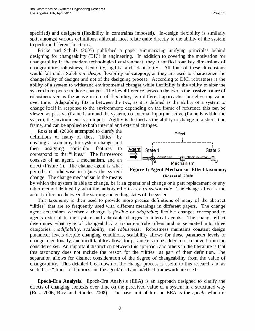
Ross et al. (2008) attempted to clarify the definitions of many of these “ilities” by creating a taxonomy for system change and then assigning particular features to correspond to the “ilities.” The framework consists of an agent, a mechanism, and an effect (Figure 1). The change agent is what perturbs or otherwise instigates the system change. The change mechanism is the means by which the system is able to change, be it an operational change or a part replacement or any other method defined by what the authors refer to as a transition rule. The change effect is the actual difference between the starting and ending states of the system.

This taxonomy is then used to provide more precise definitions of many of the abstract “ilities” that are so frequently used with different meanings in different papers. The change agent determines whether a change is flexible or adaptable; flexible changes correspond to agents external to the system and adaptable changes to internal agents. The change effect determines what type of changeability a transition rule offers and is separated into three categories: modifiability, scalability, and robustness. Robustness maintains constant design parameter levels despite changing conditions, scalability allows for those parameter levels to change intentionally, and modifiability allows for parameters to be added to or removed from the considered set. An important distinction between this approach and others in the literature is that this taxonomy does not include the reason for the “ilities” as part of their definition. The separation allows for distinct consideration of the degree of changeability from the value of changeability. This detailed breakdown of the change process is useful to this research and as such these “ilities” definitions and the agent/mechanism/effect framework are used.

Epoch-Era Analysis. Epoch-Era Analysis (EEA) is an approach designed to clarify the effects of changing contexts over time on the perceived value of a system in a structured way (Ross 2006, Ross and Rhodes 2008). The base unit of time in EEA is the epoch, which is

Figure 1: Agent-Mechanism-Effect taxonomy (Ross et al, 2008)

Effect


3

defined as a fixed period of contexts and needs in which the system operates, characterized using a set of variables. These variables can define anything that has an effect on the usage and value of the system; weather patterns, political scenarios, financial situations, operational plans, and the availability of other technologies are all potential epoch variables. Appropriate epoch variables for an analysis include key (i.e., impactful) exogenous uncertainty factors that will affect the perceived success of the system. The complete set of epochs, differentiated using these variables, can then be assembled into eras, ordered sequences of epochs creating a description of a potential progression of contexts and needs over time. This approach provides an intuitive base upon which to perform analysis of value delivery over time for systems under the effects of changing circumstances and operating conditions, an important step to take when evaluating large-scale engineering systems with long lifespans.

EEA was originally conceived with the intent for it to be used with Multi-Attribute Tradespace Exploration (MATE), which models large numbers of designs and compares their costs and utilities, represented as combinations of nonlinear functions of performance attributes (Ross et al. 2004). MATE is a powerful tool for conceptual system design, allowing for the evaluation and comparison of many different potential designs that could be chosen for development and fielding. An appropriate enumeration of a design vector is used to define the potential systems that are then modelled via a computer simulation, allowing for a more complete exploration of a larger design space than the traditional engineering practice of fleshing out a handful of potential designs and selecting from amongst them.

In addition to its function as a temporal extension of the typically static-context exploration of tradespaces, EEA can be used as an approach for considering value-over-time regardless of the underlying methodology. Treating the passage of time as a stochastic sequence of static conditions can be used to extend other common engineering analyses, including the investigation of a single point design for which time-dependent performance variables are present. This allows for potential broader application of EEA, beyond tradespace exploration.

The Five-Step Method

This paper will now present a new method, formed as an application of EEA, intended to clarify the potential for valuable changeability in candidate designs for a prospective mission undergoing analysis. EEA allows for the consideration of many future scenarios, in which different designs will have different perceived value; the ability to change a design using transition rules will therefore have value of its own, but this value is difficult to quantify due to time and context dependence. The following five-step method is proposed as an incremental approach that can be used to clarify the differences between the changeability of design alternatives and better inform strategic decision making during the design process. The five steps of the method are: 1) selection of designs; 2) calculation of changeability value; 3) aggregation of frequency distributions; 4) cross-epoch statistical breakdown; and 5) stochastic era analysis. A case example of the method will be presented in the section following this method description.

Study Setup. Initiating the method requires the proper construction of an EEA study.

To reiterate, epochs are defined as periods of time during which the system operates in a particular fixed context and set of needs. An epoch is defined by a set of epoch variables, which must be enumerated. Epoch variables should include any and all situational or operational conditions that will change over time and significantly impact the system’s delivery of value.


4

The epochs must differentiate the candidate designs in value or the results of the method will be simply a repetitious version of a static context study; for this reason, selecting value-affecting epoch variables is a critical step towards investigating the value-over-time characteristics of different designs.

1 – Selection of Designs. The first step of the method is selecting the designs of interest for

the study. Selection can take many forms depending on available time, data, and amount of detail required or desired from the study. For a full tradespace study, the number of designs selected can vary from a handful to the entire tradespace. For a more technically in-depth study, the method is equally applicable to a single point design. It is recommended that the number of selected designs be kept to no more than ten unless the purpose of the study is to simply record data for an entire tradespace. Having more than ten designs makes the results of the later steps much more difficult to process and draw conclusions from, because the method is not an optimization procedure and will not return a result that simply says what design is best. If the study has more than ten design candidates, an intelligent pre-processing to find designs of interest is valuable.

2 – Calculation of Changeability Value. This step of the method is generalizable, due

to full compatibility with any desired changeability value metric. Changeability value metrics are measures that assign a value to a design, using some means of representing the value of executing available transition options from that design. EEA is sufficiently general that it can be applied as a time-sensitive extension to any static-context study; as such, any metric that can be used to value changeability in a single context can be used across all of the epochs in the study. A number of different changeability metrics exist, from NPV of real options (Mathews and Datar 2007) to value weighted filtered outdegree (Viscito and Ross 2009), and all have positive and negative aspects. The selection of metric should be based on the available information in the study and the suitability of the metric’s assumptions for the application. The final section of this paper has additional discussion on various metrics and the development of a new mathematically robust metric. Whatever metric is selected should be used to evaluate each design selected in Step 1 in each of the generated epochs.

3 – Aggregation of Frequency Distributions. This step requires compiling the calculated

changeability values (for each design in each epoch) and presenting them as frequency distributions. The distributions can plot the valuable changeability for one design over all epochs, or for one epoch over all designs. The goal of generating these representations is to present graphs that provide an immediate, intuitive understanding of the valuable changeability available. Figure 2 shows a notional example of each of these graph types. From this quick view, we can see that Design XX shows some significant variability in valuable changeability, with a significant number of epochs in the lowest-value bin but also a few high-

Figure 2: Example Frequency Distributions


5

value performances. Epoch YY appears to be a difficult epoch in which to change effectively, with the vast majority of designs in the low-changeability region.

The conclusions that can be drawn from these plots are limited, as the insight that can be quickly collected visually is only qualitative. However, one can compare the distributions of a small set of designs simultaneously in order to understand broad similarities and differences between alternatives. One of the main reasons that it is recommended for the number of selected designs to remain under ten is to increase the ease of comparing the distributions visually. If more than ten designs are of interest, then the process can be repeated to analyze those designs as well. If probabilities of occurrence are assigned to the epochs, the design frequency distribution can be weighted into a probability distribution. This weighting can be effective in providing insight if done properly, however it is often difficult to accurately predict the probabilities of future occurrences. Probabilities should be used only if a model for changing epoch variables exists and should not be assigned heuristically without a full understanding of the potential risks by the analyst.

4 – Cross-Epoch Statistical Breakdown. The fourth step is a breakdown of the

distributions into representative statistics. This is a separate step because it represents a loss of information (e.g., shape of distribution), but it results in a quantitative basis upon which to compare designs and epochs. The main quantities that should be extracted are the order statistics of the distribution: minimum, maximum, median, and other percentiles of interest to the system analyst. Mean and variance can be calculated and compared, but carry little physical significance due to the frequency distributions not necessarily belonging to a canonical form.

Table 1 describes the changeability quartiles of three different notional designs, XX, XY, and XZ. The numbers themselves (the valuable changeability scores at a given percentile) may not mean anything out of context, as all we know for sure is that larger is better, but they do provide excellent comparisons between the designs. We can see that depending on the design philosophy or stakeholder preferences, the design of most interest from a changeability standpoint could easily be different. Design XX has the highest potential changeability value, Design XY has the highest minimum and is thus, by some measure, the safest choice, and Design XZ has the highest median valuable changeability given changing contexts. This view allows for fast, quantitative comparisons of this type, differentiating designs along whatever percentiles are most important to the analyst.

5 – Stochastic Era Analysis. The final step in the method involves stochastically sampling epochs and assembling eras (era construction) in order to better understand what change mechanisms would be used in operation, as well as how often, by each design. This analysis can be achieved quickly with a basic software model, or extremely in depth results can be gathered with a more complicated simulation. The data being collected can vary extensively by application, but will frequently include such design metrics as average lifetime, average cost spent on change in operation, and average number of changes used over a lifetime. The software implementation will depend heavily on the application, particularly with the choice of valuable

Design XX XY XZ Min 0 0.1 0

1st Quartile 0.2 0.2 0.1 Median 0.3 0.25 0.4

3rd Quartile 0.6 0.3 0.5 Max 0.7 0.4 0.6

Table 1: Cross-epoch Valuable Changeability


6

changeability metric. For example, a tradespace study with defined transition mechanisms might use an algorithm that specifies criteria that determine when a change is executed and what change is used. A real option study could use the epoch sequence in the era to create a higher-fidelity estimate of option value by including varying economic parameters into the calculation of the option’s future value stream.

The next section applies this five-step method to a satellite system tradespace study, seeking to uncover insights into design alternatives with valuable changeability.

Brief Case Study: X-TOS

Background and Setup. X-TOS is a proposed particle-collecting satellite designed to sample atmospheric density in low Earth orbit. A full MATE study was performed in 2002 to analyze potential designs for the system. For the study, 8 design variables were mapped into 7840 designs with 5 utility-generating attributes; the variables and related attributes are detailed in Table 2. Additionally, multiple-satellite configurations were tested, but not included in the final tradespace due to vastly increased cost for only marginal increased utility. Changeability was noted to be highly desirable in the X-TOS final report, because an unknown parameter (atmospheric density, which the system was designed to measure) had a large impact on the performance of the satellite.

In 2006, the X-TOS study was revived as a case study for a research effort to quantify changeability (Ross and Hastings 2006). Using the change agent-mechanism-effect framework, 8 transition rules were created allowing for the change from one design point to another. The rules are listed in Table 3. It should be noted that the “tugable” and “refuelable” designations were added as design variables, to be included at a fixed cost as enablers for the appropriate change mechanisms. The study encompasses both adaptability and flexibility, as the “burn fuel” change mechanism responds to an internal agent (adaptable), while the others respond to external agents (flexible). There is also an appreciable spread in costs, as the Burn Fuel mechanism is modelled to cost orders of magnitude less to employ, in both time and money, than the others.

Design Variable Directly Associated

AttributesApogee Lifetime, Altitude

Perigee Lifetime, Altitude

Inclination Lifetime, Altitude, Max

Latitude, Time at EquatorAntenna Gain Latency

Comm. Architecture Latency

Propulsion Type Lifetime

Power Type Lifetime

∆V Capability Lifetime

Change Mechanism

Design Requirement

Effect

Burn Fuel

Sufficient ∆VChange inclination,

decrease ∆V

Sufficient ∆VChange apogee,

decrease ∆V

Sufficient ∆VChange perigee,

decrease ∆V

Space TugTugable Change inclination Tugable Change apogee Tugable Change perigee

Refuel Refuelable Increase ∆V

Launch New Satellite

(none) Change all orbit

parameters and ∆V

Finally, 58 different epochs were generated to extend the study into epoch-era analysis. In

this case, the epochs were generated by perturbing the defined stakeholder utility preferences of

Table 2: X-TOS Design Variables Table 3: Transition Rules for X-TOS


7

the MATE study in one of four ways: adding/removing attributes, reweighting the attributes, linearizing the attribute utility curves, and altering the multi-attribute utility aggregation function. These epochs form a basis for a “what if?” analysis of the future, addressing such design process uncertainties as “What if we selected the wrong attribute set?” or “What if the stakeholder changes preferences?” (Ross et al. 2009). This is an acceptable method of generating epochs, although ideally the stakeholder would be available to re-derive his preferences for different potential scenarios in the system’s future such as a goal change or wartime conditions.

1 – Selection of Designs. For this example, we will investigate seven designs indicated as

designs of interest in the 2006 study; their features are shown in Table 4. The set can be viewed as the result of an intelligent pre-processing of the designs, filtering out many designs that are uninteresting regardless of their changeability performance. The first row, DV, indicates the assigned design number label, which is how they will be designated in this study.

2 – Calculation of Changeability Value. The valuable changeability for each design in

each epoch was calculated according to Value Weighted Filtered Outdegree (VWFO) metric, which is defined by the following equation (Viscito and Ross 2009, Hastings 2010):

VWFOim

1

N 1[H(u j

m1 uim1) Arci, j

m ]j1

N1

H = Heaviside step function N = number of designs i = origin design j = destination design Arc = transition allowed m = current time (context) m+1 = future time (context) u = utility of design

VWFO was chosen because it was designed to work in tradespace exploration with the agent-mechanism-effect change framework, which is how the system’s transition rules were defined in the 2006 study. The metric roughly corresponds to the fraction of the tradespace that is

Table 4: X-TOS Designs of Interest (Ross and Hastings, 2006)


8

accessible from the given design using change mechanisms that cost less than a given filter, counting only end states with a higher multi-attribute utility than the current design. It is worth noting that VWFO is formulated using the difference in design utilities for an unknown future epoch (m+1), corresponding to the undetermined future value of a transition anticipating an epoch shift. For the purposes of this case study, we consider epoch m+1 to be strictly the same as epoch m; this assumption simplifies the calculation into one that values reactionary change (ie, changing within epoch m in response to epoch m arising) rather than anticipatory change. This particular simplification results in little information loss when used in the five-step method since we will be considering the VWFO score for each design in each epoch; the unknown future value of the change that we are taking out of the individual VWFO calculation will be reintroduced when considering the distribution over all epochs. The actual VWFO values are not presented here, because the individual scores are not useful without the context of comparison between designs and epochs (the magnitude of VWFO is not indicative of value when considered alone, only relative to other designs and epochs).

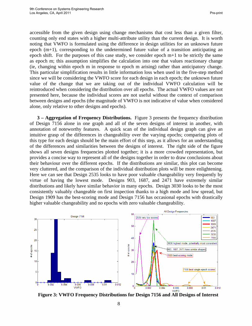
3 – Aggregation of Frequency Distributions. Figure 3 presents the frequency distribution

of Design 7156 alone in one graph and all of the seven designs of interest in another, with annotation of noteworthy features. A quick scan of the individual design graph can give an intuitive grasp of the differences in changeability over the varying epochs; comparing plots of this type for each design should be the main effort of this step, as it allows for an understanding of the differences and similarities between the designs of interest. The right side of the figure shows all seven designs frequencies plotted together; it is a more crowded representation, but provides a concise way to represent all of the designs together in order to draw conclusions about their behaviour over the different epochs. If the distributions are similar, this plot can become very cluttered, and the comparison of the individual distribution plots will be more enlightening. Here we can see that Design 2535 looks to have poor valuable changeability very frequently by virtue of having the lowest mode. Designs 903, 1687, and 2471 have extremely similar distributions and likely have similar behavior in many epochs. Design 3030 looks to be the most consistently valuably changeable on first inspection thanks to a high mode and low spread, but Design 1909 has the best-scoring mode and Design 7156 has occasional epochs with drastically higher valuable changeability and no epochs with zero valuable changeability.

Figure 3: VWFO Frequency Distributions for Design 7156 and All Designs of Interest


9

4 – Cross-Epoch Statistical Breakdown. Table 5 displays the order statistics of the distributions generated in the previous step, with the best scores highlighted in green and the worst in red. The tabular view is similar to the previous step, because it highlights features that we notice in the distribution, but it also allows for a faster and more quantitative comparison between the designs. Many of our inferences from the distributions are confirmed here; Design 1909 is consistently valuably changeable, as it has the highest VWFO for all three quartiles, and Design 7156 has both the highest minimum and maximum by a significant margin. We also reconfirm that Design 2535 possesses less valuable changeability than the other designs, as apparent from its many red boxes.

The mean and standard deviation are included in the bottom two rows of the table to illustrate an important point previously mentioned: the mean is a misleading measure of central tendency and should be used with caution. Design 7156 scores the highest mean, but only because, as the design with the highest maximum, its high outliers pull up the average. Meanwhile, the standard deviation tells us little information about value: as we can see, the interesting Design 7156 scores worst in standard deviation, and the unremarkable Design 3030 scores best.

When considering more than a handful of designs, comparing the frequency distributions by inspection becomes unwieldy. When presented in table form, the relevant information becomes much easier to see. Heat maps of the table, highlighting very good scores on a continuous spectrum (as opposed to the best/worst colouring scheme shown here), have the potential to reintroduce a visual aid to ascertaining value that is lost in the previous step.

Design # 903 1687 1909 2471 2535 3030 7156

Min 0 0 0 0 0.000128 0.000383 0.001914

1st Quart. 0.002424 0.002424 0.002807 0.002169 0.000638 0.002551 0.002424

Median 0.002551 0.002807 0.003062 0.002679 0.000765 0.002551 0.002551

3rd Quart. 0.002807 0.002934 0.003062 0.002807 0.000765 0.002551 0.002934

Max 0.003955 0.00421 0.003572 0.004082 0.005485 0.002807 0.017987

Mean 0.002463 0.002613 0.002833 0.00249 0.000798 0.00245 0.003132

Std Dev 0.000648 0.000667 0.000629 0.000655 0.000691 0.00048 0.002268

5 – Stochastic Era Analysis. A simple era constructor and decision algorithm were

created in MATLAB® for the purposes of this case study. The era construction and transition decision rules used are as follows:

1. Each epoch is equally likely to occur 2. An epoch’s duration is a geometric random variable with p=0.5, each trial counts as 1 year 3. The system is a success if it operates for 15 years without falling below a utility of 0.4 4. If an epoch arises where the current design has a utility <0.4, two things can happen:

a. The least expensive transition to a design with utility >0.4 is taken b. If no such transition exists, the system fails and does not record as a success

Table 5: Statistical Breakdown of X-TOS VWFO Data


10

This is an exceedingly simple era analysis model, but it encompasses the basic features of in-operation system change, responding to decreases in value with some logical process. If more time is put into designing the decision model, more informative and realistic results can be achieved. For example, penalty costs for failure can be implemented or more effective decision making algorithms can be applied, such as “move as close to the tradespace Pareto Front in the new epoch as possible, subject to cost constraints”. The decision algorithm can also vary based on the current epoch, as the situation may dictate a particular response.

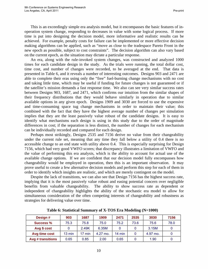
An era, along with the rule-invoked system changes, was constructed and analyzed 1000 times for each candidate design in the study. As the trials were running, the total dollar cost, time cost, and number of changes were recorded, to be averaged at the end. That data is presented in Table 6, and it reveals a number of interesting outcomes. Designs 903 and 2471 are able to complete their eras using only the “free” fuel-burning change mechanisms with no cost and taking little time, which may be useful if funding for future changes is not guaranteed or if the satellite’s mission demands a fast response time. We also can see very similar success rates between Designs 903, 1687, and 2471, which confirms our intuition from the similar shapes of their frequency distributions that they would behave similarly in operation due to similar available options in any given epoch. Designs 1909 and 3030 are forced to use the expensive and time-consuming space tug change mechanisms in order to maintain their value; this combined with the fact that they have the highest average number of changes per simulation implies that they are the least passively value robust of the candidate designs. It is easy to identify what mechanisms each design is using in this study due to the order of magnitude differences in cost; if the separation is less distinct, the number of changes for each mechanism can be individually recorded and compared for each design.

Perhaps most strikingly, Designs 2535 and 7156 derive no value from their changeability under the current rule set, meaning that any time they fall below a utility of 0.4 there is no accessible change to an end state with utility above 0.4. This is especially surprising for Design 7156, which had very good VWFO scores; that discrepancy illustrates a limitation of VWFO and the value of performing this era analysis, which is the ability to account for actual use of the available change options. If we are confident that our decision model fully encompasses how changeability would be employed in operation, then this is an important observation. It may prove useful to create a few alternative decision models and perform this step for each of them in order to identify which insights are realistic, and which are merely contingent on the model.

Despite the lack of transitions, we can also see that Design 7156 has the highest success rate, implying that it is the most passively value robust and easing potential concern over negligible benefits from valuable changeability. The ability to show success rate as dependent or independent of changeability highlights the ability of the stochastic era model to allow for simultaneous consideration of the often competing interests of changeability and robustness as strategies for delivering value over time.

Design # 903 1687 1909 2471 2535 3030 7156

Success % 75.3 75.8 75.0 75.2 73.6 75.6 78.0

Avg $ cost 0 2.49K 6.35M 0 0 3.15M 0

Avg time cost 13 min 17 min 4.27 mo. 14 min 0 4.97 mo. 0

Avg # transitions 0.65 0.85 2.00 0.65 0 1.90 0

Table 6: Statistical Summary of X-TOS Era Modeling (N=1000)


11

Discussion and Future Research

Overall, the method described in this paper was shown to provide key insights into the value of changeability over the lifetime of a system and subject to changing contexts. The ability to investigate time-dependent and context-dependent value of changeability is critical, as the inevitability of changing context is one of the main incentives for designing a changeable system. Moreover, the method is developed in such a way as to allow for accessible comparison of different candidate designs, indicating potential usefulness in the method’s application to the design process.

Considerable concern remains over the choice of metric for the calculation of valuable changeability, the second step in this method. One of the strengths of this method lies in its ability to accommodate any valuable changeability metric that can be evaluated in a static context and extrapolate it across changing contexts. However, there currently does not exist a fundamental metric for valuable changeability that is both mathematically sound and appropriate across most or all applications. In the case study presented in this paper, value weighted filtered outdegree was chosen due to its ease of calculation and its prior use with epoch-era analysis. An example concern with VWFO is the lack of accounting for degree of value: all positive-value changes are weighted equally, rather than considering both the weighted value of a single change and the counting value of the total number of changes in a design. Attempts to weight the function by utility are met with mathematical roadblocks, as the multi-attribute utility scale is neither linear nor commensurate between epochs.

Another example value metric that has been applied to changeability is the net present value (NPV) of real options. Real options are an extension of classical financial options, valued using a modified Black-Scholes equation to account for differences between financial options and the reality of holding options on physical systems. Many of these assumptions are questionable, such as treating the option as fully liquid and traded on a market with perfect information, but even if they are accepted, there are a number of conceptual limitations in applying real options to engineering systems. For example, large systems such as satellites are designed to be built once and are evaluated on their performance. Because the language of real options is the language of finance, all value is presented in monetary form, and it can be extremely difficult to quantify system utility as a dollar amount. Despite these limitations, real options have been used to gain insight into engineering changeability and the field has the potential for future growth (Mathews and Datar 2007, Pierce 2010).

There are many other metrics that have been researched and suggested as methods for valuing changeability, but they all suffer from similar problems as the above two. Research has been performed into design space based changeability metrics (Swaney and Grossmann 1985), parameter space metrics (Olewnik et al. 2006), and design structure matrices (Kalligeros et al. 2006) as attempts to properly quantify or value the changeability or the degree of change propagation in engineering systems. Unfortunately, these separate research threads have all been focused on a particular application, resulting in metrics and methods that are often inappropriate or impossible to use in a different field. Another common thread of complications among these research paths is the difficulty in assigning a concrete definition of value to changeability, as value is an abstract and fluid concept. As such, common measures of static value (e.g., multi-attribute utility) are based on non-physical constructs (e.g., stakeholder preferences) that can vary over time and context, invalidating their use as commensurate value-over-time metrics.

Ongoing research seeks to offer a general and robust alternative to existing valuable changeability metrics. The method in this paper will remain applicable to any choice of metric,


12

but the inclusion of a metric designed explicitly for use in EEA has the potential to create a more complete, powerful method overall that spans a greater part of the design process and provides more insight for changeability comparisons between designs. The current direction of the research continues to employ the agent-mechanism-effect framework of change, which is sufficiently general to provide a common starting point for most engineering disciplines. The research will also focus on resolving the weighting-versus-counting issue mentioned above. One possibility is the development of a valuable changeability metric that is applied to a single transition rule for the weighting aspect and then is aggregated across all the rules for a design to include the counting aspect into a single design changeability score. This new metric would allow for additional interesting design tradeoffs, as it would be possible to then calculate the dependence of a single design’s valuable changeability on a given change mechanism. Knowing the value of each mechanism, which is often an optional package on the base architecture, could allow for quantitative tradeoffs between different changeability-enabling options.

Achieving the end goal, to have a generalizable metric and method for analyzing engineering system valuable changeability, would significantly open up the potential for systems to be designed with changeability as an effective means for delivering sustained value over time. The metric should assign the values and then the method should take those values and analyze them in such a way as to allow for changeability to be compared effectively between designs and traded off against other value-preserving strategies such as robustness. The method presented in this paper has been shown to be a promising tool for valuable changeability comparison, so with only the lack of a robust metric remaining, there is potential for this research topic to contribute to the practical understanding of changeability in the field within the near future.

Acknowledgments

The authors of this paper are grateful for the sponsorship of this research by the Defense Advanced Research Projects Agency (DARPA). The views expressed in this paper are those of the authors and are not endorsed by the sponsor

References

Fricke, E. and A.P. Schulz, “Design for changeability (DfC): Principles to enable changes in

systems throughout their entire lifecycle,” Systems Engineering, vol. 8, 2005, pp. 342-359. Hastings, D.E., “Analytic Framework for Adaptability,” Presentation to Defense Science Board,

2010. Kalligeros, K., O.D. Weck, and R.D. Neufville, “Platform identification using Design Structure

Matrices,” Sixteenth Annual International Symposium of the International Council On Systems Engineering INCOSE, 2006.

Mathews, S. and V. Datar, “A Practical Method for Valuing Real Options: The Boeing Approach,” Journal of Applied Corporate Finance, vol. 19, 2007, pp. 95-104.

Olewnik, A. and K. Lewis, “A decision support framework for flexible system design,” Journal of Engineering Design, vol. 17, 2006, pp. 75-97.

Pierce, J.G., “Designing Flexible Engineering Systems Utilizing Embedded Architecture Options,” Vanderbilt Systems Engineering PhD thesis, 2010.

Ross, A.M., Hastings, D.E., Warmkessel, J.M., and Diller, N.P., “Multi-Attribute Tradespace Exploration as a Front-End for Effective Space System Design,” AIAA Journal of Spacecraft and Rockets, Jan/Feb 2004.


13

Ross, A.M., “Managing Unarticulated Value: Changeability in Multi-Attribute Tradespace Exploration,” MIT Engineering Systems Division PhD thesis, 2006.

Ross, A.M. and D.E. Hastings, “Assessing Changeability in Aerospace Systems Architecting and Design Using Dynamic Multi-Attribute Tradespace Exploration,” AIAA Space 2006, 2006, pp. 1-18.

Ross, A.M., D.H. Rhodes, and D.E. Hastings, “Defining Changeability : Reconciling Flexibility , Adaptability , Scalability , Modifiability , and Robustness for Maintaining System Lifecycle Value,” Systems Engineering, vol. 11, 2008, pp. 246-262.

Ross, A.M. and D.H. Rhodes, “Using Natural Value-Centric Time Scales for Conceptualizing System Timelines through Epoch-Era Analysis,” INCOSE 2008, 2008.

Ross, A.M., D.H. Rhodes, and D.E. Hastings, “Using Pareto Trace to Determine System Passive Value Robustness,” 2009 3rd Annual IEEE Systems Conference, Mar. 2009, pp. 285-290.

J. Saleh, G. Mark, and N. Jordan, “Flexibility: a multi-disciplinary literature review and a research agenda for designing flexible engineering systems,” Journal of Engineering Design, vol. 20, Jun. 2009, pp. 307-323.

Swaney, R.E. and I.E. Grossmann, “An Index for Operational Flexibility in Chemical Process Design,” Chemical Engineering, vol. 31, 1985, pp. 631-641.

Viscito, L. and A.M. Ross, “Quantifying Flexibility in Tradespace Exploration : Value Weighted Filtered Outdegree,” AIAA Space 2009, 2009, pp. 1-9.

Biography

Matthew Fitzgerald is a candidate for an S.M. in the Department of Aeronautics and Astronautics at the Massachusetts Institute of Technology. He is affiliated with the Systems Engineering Advancement Research Initiative and performs research on the topics of epoch-era analysis, system design metrics, and data visualization / design process tools.

Dr. Adam M. Ross is a research scientist in the Engineering Systems Division at the

Massachusetts Institute of Technology. He has professional experience working with government, industry, and academia. He holds a bachelor’s degree in Physics and Astrophysics from Harvard University, two master’s degrees in Aerospace Engineering and Technology & Policy, and a doctoral degree in Engineering Systems from MIT. He advises ongoing research in systems design and selection methods, tradespace exploration, managing unarticulated value, designing for changeability, value-based decision analysis, and systems-of-systems engineering. He has published over 50 papers in space systems design, systems engineering, and tradespace exploration.

Dr. Donna H. Rhodes is director of the MIT Systems Engineering Advancement Research Initiative (SEAri). She is a senior lecturer and principal research scientist in Engineering Systems at MIT. She holds a Ph.D. in Systems Science from the T.J. Watson School of Engineering at SUNY Binghamton. Prior to joining MIT, Dr. Rhodes had 20 years of experience in the aerospace, defense systems, systems integration, and commercial product industries. She is a Past President and Fellow of the International Council on Systems Engineering (INCOSE), and recipient of the INCOSE Founders Award.


a method using epoch-era analysis to identify...

Documents