a methodology for placement-aware partitioning · effectively in order to reduce the design...

A Methodology for Placement-Aware Partitioning

WEI-KAI CHENG, TSU-YUN HSUEH, JUI-HUNG HUNG, TSAI-MING HSIEH, MELY CHEN CHI

Department of Information & Computer Engineering Chung Yuan Christian University

Chung-Li, Taiwan 32023 {wkcheng, g9877014, g9777036, hsieh, mlchen}@cycu.edu.tw

Abstract: - Circuit partition is the first stage of physical design. As the improvement of semiconductor technique, the number of transistors increases rapidly in a VLSI design. Therefore, how to partition a circuit effectively in order to reduce the design complexity becomes a crucial problem. In this paper, we propose a placement-aware partition methodology to reduce the total wire length after cell placement and global routing. A 2-way partitioning algorithm developed previously has been proved to be effective for the 3D IC partition problem. By the application of 2-way partitioning algorithm and a set of terminal propagation rules proposed in this paper, we can take into account the external interconnections of the target partition region effectively, and calculate the gain of partition precisely, such that the wire length could be minimized. A set of benchmarks from the 2011 ISPD contest are used to test our methodology. Experimental results show that in comparison with previous work, our methodology reduces the total wire length after placement in terms of both HPWL and STWL, and also reduces the real length of routing wires after global routing effectively. Key-Words: - placement-aware partition, terminal propagation, EIA-coarsening, HPWL, STWL

1 Introduction As the scale of design complexity and progress of manufacture process in semiconductor, the number of transistors in an integrated circuit increases rapidly. Hence, partitioning the circuits efficiently and placing the partitioned circuits in proper positions become a crucial problem in the design of VLSI.

Circuit partitioning is the first stage of physical design. The goal of partitioning is to minimize the number of cut lines between the partitioned sub-circuits. Among the previous researches for circuit partitioning, hMetis [4][5][6] developed by George Karypis et al. is the most efficient one for the k-way partition problem. Firstly, it reduced the size of netlist by cell coarsening. The coarsening algorithms they proposed including edge coarsening (EC), hyperedge coarsening (HEC), modified hyperedge coarsening (MHEC), and first choice (FC). Then in the second stage, hMetis applied the FM [7] methodology and performed partitioning refinement through the un-coarsening procedure. By this top-down approach, hMetis can efficiently reduce the number of cut lines for the k-way partitioning problem.

Except for the general two dimensional circuit partitioning problem, there also have some researches [8][9][10][11][12] for 3D IC partitioning problem. The modified coarsening and partitioning

approaches have also been proved to be useful for the 3D IC partitioning problem [11], and got the best award for the 2011 CAD contest in Taiwan [1].

After circuit partitioning, we need to assign each logic cell to a proper position on the cell rows. There have been many researches on the cell placement problem [13][14][18][19][21]. Among all these different types of methodologies, the partitioning based approach is widely used [13][14][18], and is shown to be efficient for interconnection and wire length reduction. In the partitioning-based cell placement approaches, an algorithm partitions the circuit recursively, until the numbers of logic cells in all the sub-circuits do not exceed the constrains of area or routing capacity. Their objective is to place the logic cells with strong interconnections in the same sub-region, and reduce the number of cut lines between all sub-regions.

In the recursive process of partitioning-based placement, how to take into account the effect of external interconnections for a target sub-region is a crucial problem. Dunlop and Kernighan [13] proposed a terminal propagation methodology to resolve this problem. External cells that have interconnections with the target sub-region are selected. Then their coordinates are projected onto the boundaries of the target sub-region. Based on these projected data, partitioning-based placement algorithm can minimize the total wire length,

WSEAS TRANSACTIONS on CIRCUITS and SYSTEMSWei-Kai Cheng, Tsu-Yun Hsueh, Jui-Hung Hung, Tsai-Ming Hsieh, Mely Chen Chi

E-ISSN: 2224-266X 13 Issue 1, Volume 12, January 2013

including inter and intra connections of the target sub-region.

For the other partitioning-based related researches, Suaris and Kedem [14][15][16][17] proposed a quadrisection-based placement approach to partition the circuit quarterly. Each time an element with the largest gain is selected and moved to the best sub-region. This process continued recursively until each cell finds a position for placement.

Based on the quadrisection methodology, Huang and Kahng [18] proposed a four-way partitioning algorithm. It can take into account the external interconnections without the need of terminal propagation. In the four sub-regions, by analyzing the distribution of cells on the same net, a lookup table method is applied to obtain a cost value. From this cost value, the gain of moving a cell to another sub-region can be calculated. The effect of external cells on the partitioning sub-region could also be calculated by the lookup table method as well.

Research [21] utilized hMetis [4][5][6] to reduce the number of cut lines at each level of partitioning, and a post bin swapping procedure is applied to reduce the wire length of interconnections. By defining a cost function to calculate the weight of each net, a matrix formulation is proposed to obtain the position for each cell placement.

In this paper, we propose a methodology for the placement-aware partitioning problem. By the application of 2-way partitioning algorithm and a set of terminal propagation rules proposed, we could minimize the wire length effectively. Experimental results show that in comparison with previous work [13], our methodology reduces the total wire length after placement in terms of both HPWL and STWL, and also reduces the real length of routing wires after global routing effectively.

The rest of this paper is organized as follows. In section 2, we introduce our motivation for considerations of external interconnections and gain estimation of partitioning. Section 3 gives the problem formulation and the program flow. In section 4, we propose a placement-aware partitioning algorithm. Section 4 gives a description of our global placement methodology. In section 6, we show the experimental results for the effect of our methodology in terms of wire length minimization. Finally, we draw the concluding remarks in section 7.

2 Motivation In this section, we describe the motivations of our placement-aware partitioning algorithm, including

the problem of terminal propagation rules and the gain estimation of the placement-aware FM algorithm. 2.1 Terminal Propagation The terminal propagation methodology proposed by Dunlop and Kernighan [13] can resolve the problem of external interconnections. When cells are distributed as shown in Fig. 1(a), and region R is the target partitioning region, cells in the L1 region will be projected onto the boundary of region R and marked as point p as shown in Fig. 1(b). By considering the position of projected point during partitioning, cells in region R will be placed to the R1 sub-region in order to have shorter wire length for interconnection as shown in Fig. 1(b).

Fig. 1: Example of terminal propagation.

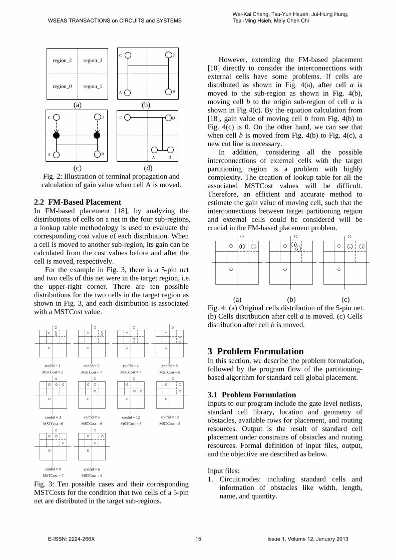
However, for the example in Fig. 2, four cells

are distributed in the four sub-regions (region_0 ~ region_3 in Fig. 2(a)) and connected by a 4-pin net as shown in Fig. 2(b). If cells in region_2 and region_3 have finished partitioning, and the target partitioning sub-regions are region_0 and region_1, cells in region_2 and region_3 will be projected onto the boundary of region_0 and region_1, respectively, as shown in Fig. 2(c). Then, cells in region_0 and region_1 will be partitioned by the FM algorithm. After calculation, the value of gain is 0 when cell A is moved to region_1; i.e. the number of cut lines will not be changed when cell A is moved from region_0 to region_1. But as shown in Fig. 2(d), when cell A is moved, there is no cut line between region_0 and region_1. This is because that in the routing stage, the L-shape routing strategy could be applied such that a connection wire can pass through region_1, region_3 and region_2 directly, to obtain the shortest routing path. Hence, the number of cut lines can be reduced from two to one, i.e. the value of gain is 1 when cell A is moved from fegion_0 to region_1. Therefore, the terminal propagation rules proposed in [13] need to be modified to take into account the interconnections with external cells precisely.



region_0 region_1

region_2 region_3

B

D

A

C

(a) (b)

A B

C D

B

D

A

C

(c) (d)

Fig. 2: Illustration of terminal propagation and calculation of gain value when cell A is moved.

2.2 FM-Based Placement In FM-based placement [18], by analyzing the distributions of cells on a net in the four sub-regions, a lookup table methodology is used to evaluate the corresponding cost value of each distribution. When a cell is moved to another sub-region, its gain can be calculated from the cost values before and after the cell is moved, respectively.

For the example in Fig. 3, there is a 5-pin net and two cells of this net were in the target region, i.e. the upper-right corner. There are ten possible distributions for the two cells in the target region as shown in Fig. 3, and each distribution is associated with a MSTCost value.

confid = 1

MSTCost = 5

confid = 2

MSTCost = 7

confid = 4

MSTCost = 7

confid = 8

MSTCost = 8

confid = 3

MSTCost =6

confid = 5

MSTCost = 6

confid = 12

MSTCost = 8

confid = 10

MSTCost = 8

confid = 9

MSTCost = 7

confid = 6

MSTCost = 9 Fig. 3: Ten possible cases and their corresponding MSTCosts for the condition that two cells of a 5-pin net are distributed in the target sub-regions.

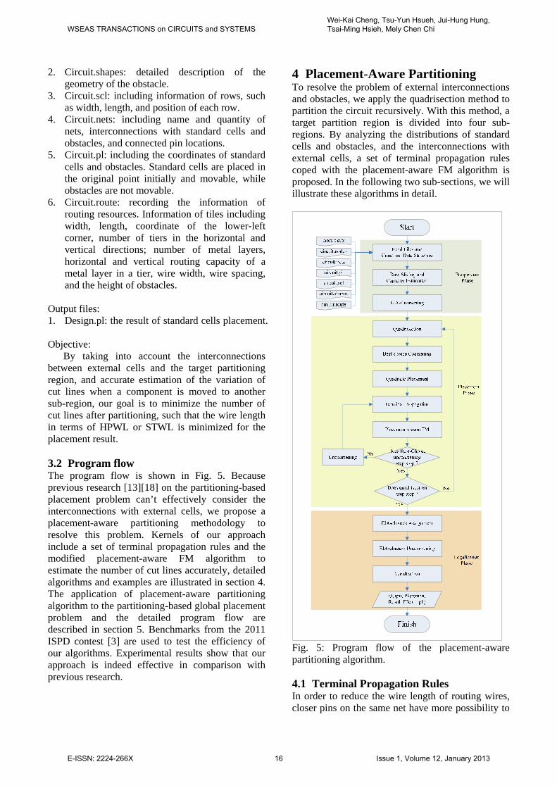
However, extending the FM-based placement

[18] directly to consider the interconnections with external cells have some problems. If cells are distributed as shown in Fig. 4(a), after cell a is moved to the sub-region as shown in Fig. 4(b), moving cell b to the origin sub-region of cell a is shown in Fig 4(c). By the equation calculation from [18], gain value of moving cell b from Fig. 4(b) to Fig. 4(c) is 0. On the other hand, we can see that when cell b is moved from Fig. 4(b) to Fig. 4(c), a new cut line is necessary.

In addition, considering all the possible interconnections of external cells with the target partitioning region is a problem with highly complexity. The creation of lookup table for all the associated MSTCost values will be difficult. Therefore, an efficient and accurate method to estimate the gain value of moving cell, such that the interconnections between target partitioning region and external cells could be considered will be crucial in the FM-based placement problem.

(a) (b) (c) Fig. 4: (a) Original cells distribution of the 5-pin net. (b) Cells distribution after cell a is moved. (c) Cells distribution after cell b is moved.

3 Problem Formulation In this section, we describe the problem formulation, followed by the program flow of the partitioning-based algorithm for standard cell global placement. 3.1 Problem Formulation Inputs to our program include the gate level netlists, standard cell library, location and geometry of obstacles, available rows for placement, and routing resources. Output is the result of standard cell placement under constrains of obstacles and routing resources. Formal definition of input files, output, and the objective are described as below. Input files: 1. Circuit.nodes: including standard cells and

information of obstacles like width, length, name, and quantity.



2. Circuit.shapes: detailed description of the geometry of the obstacle.

3. Circuit.scl: including information of rows, such as width, length, and position of each row.

4. Circuit.nets: including name and quantity of nets, interconnections with standard cells and obstacles, and connected pin locations.

5. Circuit.pl: including the coordinates of standard cells and obstacles. Standard cells are placed in the original point initially and movable, while obstacles are not movable.

6. Circuit.route: recording the information of routing resources. Information of tiles including width, length, coordinate of the lower-left corner, number of tiers in the horizontal and vertical directions; number of metal layers, horizontal and vertical routing capacity of a metal layer in a tier, wire width, wire spacing, and the height of obstacles.

Output files: 1. Design.pl: the result of standard cells placement.

Objective:

By taking into account the interconnections between external cells and the target partitioning region, and accurate estimation of the variation of cut lines when a component is moved to another sub-region, our goal is to minimize the number of cut lines after partitioning, such that the wire length in terms of HPWL or STWL is minimized for the placement result. 3.2 Program flow The program flow is shown in Fig. 5. Because previous research [13][18] on the partitioning-based placement problem can’t effectively consider the interconnections with external cells, we propose a placement-aware partitioning methodology to resolve this problem. Kernels of our approach include a set of terminal propagation rules and the modified placement-aware FM algorithm to estimate the number of cut lines accurately, detailed algorithms and examples are illustrated in section 4. The application of placement-aware partitioning algorithm to the partitioning-based global placement problem and the detailed program flow are described in section 5. Benchmarks from the 2011 ISPD contest [3] are used to test the efficiency of our algorithms. Experimental results show that our approach is indeed effective in comparison with previous research.

4 Placement-Aware Partitioning To resolve the problem of external interconnections and obstacles, we apply the quadrisection method to partition the circuit recursively. With this method, a target partition region is divided into four sub-regions. By analyzing the distributions of standard cells and obstacles, and the interconnections with external cells, a set of terminal propagation rules coped with the placement-aware FM algorithm is proposed. In the following two sub-sections, we will illustrate these algorithms in detail.

Fig. 5: Program flow of the placement-aware partitioning algorithm. 4.1 Terminal Propagation Rules In order to reduce the wire length of routing wires, closer pins on the same net have more possibility to



be connected by a routing wire. By this characteristic, external pins that are closer to the target partition region have more possibility to be connected with pins inside the target region by a routing wire, and hence their distributions have the largest impact on the positions of cells placement inside the target region. Therefore, before terminal propagation, we firstly find external pins that have the smallest Manhattan distance with the four boundary lines of the target region. For example, Fig. 6(a) shows the distribution of all external pins and their distance to the boundaries. Fig. 6(b) shows that four of them have the shortest distance to the four boundaries are selected.

After external pins are selected, we analyze their distributions and their interconnect relationships with the four sub-regions. Different from the projection methodology in research [13], when all external pins are connected by the shortest routing path as shown in Fig. 7(a), we add dummy cells in the sub-regions that the shortest routing path across as shown in Fig. 7(b), such that the distributions of external pins and dummy cells have the least number of cut lines inside the target region. Therefore, in the phase of placement-aware FM partitioning described in the next sub-section, we can take into account the impact of external interconnections simultaneously, and minimize the number of cut lines between all sub-regions.

Fig. 6: (a) Distribution of external pins outside the target region. (b) External pins that have the shortest distances to the four boundaries of the target region.

(a) (b) Fig. 7: (a) Shortest routing path of the external pins. (b) Dummy cells on the shortest routing path.

Distribution analysis of external pins and

terminal propagation rules are described as below, there are six steps in total.

Step 1: Check the distribution of obstacles. If an obstacle has connection relationships with cells inside the target region, and the connected pin is also residing in the target region, a dummy cell is added to the corresponding sub-region.

Step 2: Check whether there are external pins in all the four corners as shown in Fig. 8(a). If there exists this condition, select any two adjacent sub-regions to add dummy cells as shown in Fig. 8(b). Otherwise, continue the next projection step.

Step 3: Check whether there are external pins in three of the four corners as shown in Fig. 9(a). If there exists this condition, select any one projected sub-region to add a dummy cell as shown in Fig. 9(b). Otherwise, continue the next projection step.

(a) (b) Fig. 8: Illustration of adding dummy cells when all the four corners have external pins.

(a) (b)

Fig. 9: Illustration of adding dummy cells when three of the four corners have external pins.

Step 4: Check whether there exists two adjacent boundaries that all have two external pins as shown in Fig. 10(a). If there exists this condition, add a dummy cell in the projected sub-region as shown in Fig. 10(b) and mark the selected external pins. Then, continue with the next step to judge the distribution of remaining external pins.

Step 5: Manage the projection of single external pin. If there is only one external pin for any one of the four boundaries, add a dummy cell to the projected sub-region. An example for this type of projection is shown in Fig. 11. After this step, selected external pins are also marked, and continue with the next step for the remaining external pins.



Step 6: Manage the projection of double external pins. When the distribution of remaining external pins is similar to one of that in Fig. 12, the first thing is to check whether or not the adjacent sub-regions had added any dummy cell previously. If any dummy cell had already added to the adjacent sub-regions, no additional dummy cell is need. Otherwise, check whether any dummy cell had added to the distant sub-regions. If both the two distant sub-regions have or do not have dummy cell simultaneously, as shown in Fig. 13(a) and Fig. 13(b), any of the two adjacent sub-regions is selected to add the dummy cell. Otherwise, the adjacent sub-region that is near to the dummy cell in the distant sub-region is selected to add the dummy cell as shown in Fig. 13(c).

(a) (b)

Fig. 10: Illustration of adding dummy cells when there are two adjacent boundaries that all have two external pins.

(a) (b)

Fig. 11: Illustration of adding dummy cells for single point projection.

(a) (b)

Fig. 12: The cases that two external pins on the same boundary or in the adjacent corners.

By the six terminal propagation rules described above, we guarantee that all the external pins and projected dummy cells can be connected with the shortest routing path, and the number of cut lines between sub-regions can be minimized.

(a) (b)

(c) Fig. 13: Illustration of adding dummy cells when there are two external pins on the same boundary. 4.2 Placement-aware FM Algorithm After the application of terminal propagation to reflect the connections with external pins, the distribution of cells and dummy cells are used to direct the partitioning of the placement-aware FM algorithm proposed in the sub-section, such that we can take into account the external interconnections and minimize the number of cut lines between sub-regions.

Traditionally, FM algorithm uses k-way partitioning for performance refinement. However, based on some researches on the 3D IC partitioning [10][11] and the results of 2011 IC/CAD Contest, Taiwan (Problem B2 from ITRI [2]), we find that the performance of successive 2-way partitioning is better than that of k-way partitioning in either the number of cut lines or the time complexity. Therefore, we use successive 2-way partitioning for the FM algorithm, and propose a new placement-aware partitioning methodology.

In each time of the 2-way partitioning, we apply the placement-aware FM algorithm targeted to two sub-regions. Because there will be more number of cut lines when connected cells are distributed in the diagonal direction, the placement-aware FM algorithm is applied for the diagonal sub-regions firstly, then for the adjacent sub-regions.

The major improvement of placement-aware FM over previous partitioning methodology is in the calculation of gain value, such that the number of cut lines can be estimated accurately when connected cells are distributed in different sub-regions. For the example in Fig. 14(a), suppose there are four clusters c0, c1, c2, and c3, cell a is in cluster c1, cell b is in cluster c3, a and b are connected by a net. When cell a is moved from c1 to



c0, estimated gain value in traditional partitioning is 0, i.e. there is no influence on the number of cut lines. However, if the four clusters are placed in four sub-regions as shown in Fig. 14(b), due to the physical position and distribution of cells, the gain value should be -1 when cell a is moved from c1 to c0, i.e. one additional cut line is added.

The placement-aware partitioning algorithm is described as below. Firstly, the four sub-regions are enumerated as the order shown in Fig. 14(b). Then, the calculation of gain value is divided into four cases as shown in Fig. 15.

Fig. 14: (a) Gain calculation of previous partitioning. (b) Gain calculation of placement-aware FM partitioning.

The first case deals with the condition when the partitioning sub-regions are in the diagonal direction, and the pre-process of this condition is shown in Fig. 16. By the concept in 3D IC partitioning, we can transform the planner cells distribution into a 3D structure with three layers. Top and bottom layers of the 3D structure represent the partitioning sub-regions in the diagonal direction, and the other two sub-regions are mapped to the middle layer of the 3D structure. For the example in Fig. 17, Fig. 17(c) and Fig. 17(d) are the 3D structure mappings of Fig. 17(a) and Fig. 17(b), respectively. In this example, there is no cell in the middle layer. Therefore, parameter weight is set to 2 as shown in line 7 of Fig. 16. This means that for any cell moved between the sub-regions in the diagonal direction, the change of

gain value is a multiple of 2 when there is no connected cell in the other two sub-sections.

clusterN[T_index]--;

if ( the partitioning area is (0,3) or (1,2) ) Setup_Case1();else if ( CheckSpecialCase() ) Setup_Case2(); else if ( the partitioning area is (0,1) or (2,3)) Setup_Case3(); else Setup_Case4();

CountGain( updateCell );

clusterN[T_index]++;

updateCell

1.2.3.4.5.6.7.8.9.10.11.12.13.14.

F_index ：the area before cell A moved T_index ：the area after cell A movedfrom_mN ：the number of cells on a net in the from-area (including dummy cell)to_mN ：the number of cells on a net in the to-area (including dummy cell)clusterN[] ：distribution of the number of cells on a net in the four areas (including dummy cell)weight ：the unit variation of gain valueupdateCell ：the cell which need update gain valueupdateCell.index：which area of this cell belong

Fig. 15: Algorithm for calculation of gain value.

from_mN = clusterN[Findex];to_mN = clusterN[Tindex];

mN = clusterN[0] + clusterN[1] + clusterN[2] + clusterN[3] - clusterN[Findex] - clusterN[Tindex];

if( mN == 0 ) weight = 2;else weight = 1;

1.2.3.4.5.6.7.8.

Fig. 16: The pre-process when partitioning sub-regions are in the diagonal direction.

a

b

c

0 1

2 3

ab

c

0

3

1、2

b

c

0 1

2 3

a

a

b

c

0

3

1、2

(a) (b)

(c) (d) Fig. 17: Illustration of transferring the 2D placement to the 3D IC structure in the diagonal direction.



The second case occurs when either before or after a cell is moved, the net connected to the moved cell having cells distributed in all the four sub-regions. The judgment method is shown in Fig. 18, and the pre-process of this condition is shown in Fig. 19. Similar as the first case, we transform the planner cells distribution into a 3D structure with three layers. Top and bottom layers of the 3D structure represent the partitioning sub-regions, and the other two sub-regions are mapped to the middle layer of the 3D structure. For the example in Fig. 20, before cell a is moved, all cells connected to the same net are distributed in all the four sub-regions, and the partitioning sub-regions are 0 and 1.

Fig. 18: Judgement of the special case.

Fig. 19: Pre-process of the special case.

a

c

0 1

2 3

a

c

b

0

1

2、3

b

d

d

Fig. 20: Illustration of transferring the 2D placement to the 3D IC structure for the special case.

For the remaining two cases, partitioning sub-regions are the left-right sub-regions and the top-down sub-regions, respectively. The pre-processes of these two conditions are shown in Fig. 21 and Fig. 22, respectively. In these two cases, there are only two layers when they are transferred into the 3D structures.

After finish the cases judgment and related pre-process, the algorithm proposed in Fig. 23 is used to update the gain value of the moved cell.

Fig. 21: The pre-process when partitioning sub-regions are in the adjacent horizontal direction.

if( F_index == 0 || F_index == 1 ) { from_mN = clusterN[0] + clusterN[1]; to_mN = clusterN[2] + clusterN[3];}else { from_mN = clusterN[2] + clusterN[3]; to_mN = clusterN[0] + clusterN[1];}

partitioning the area 0,2 or 1,3

1.2.3.4.5.6.7.8.

Fig. 22: The pre-process when partitioning sub-regions are in the adjacent vertical direction.

Fig. 23: Calculation of updated gain value.

In summary, with the dummy cells added in the terminal propagation rules, we can take into account the impact of external interconnections and obstacles precisely by analyzing the distributions of real and dummy cells. The gain value can be calculated accurately by our placement-aware FM algorithm, such that the number of cut lines between sub-regions is minimized.



5 Partitioning-based Placement In this section, we firstly give an overview of the global placement algorithm. Then, we introduce the methodology to reduce the problem size by EIA-coarsening in detail. Finally, integration of the placement-aware partitioning algorithm into the global placement flow is described. 5.1 Global Placement Overview The overall program consists of three phases, pre-process, placement, and legalization as shown in Fig. 5. After read the six input files and construct the data structure, the main tasks of pre-process phase are row slicing and capacity estimation. Because the positions of obstacles are non-movable, we slice the rows according to the distributions of obstacles.

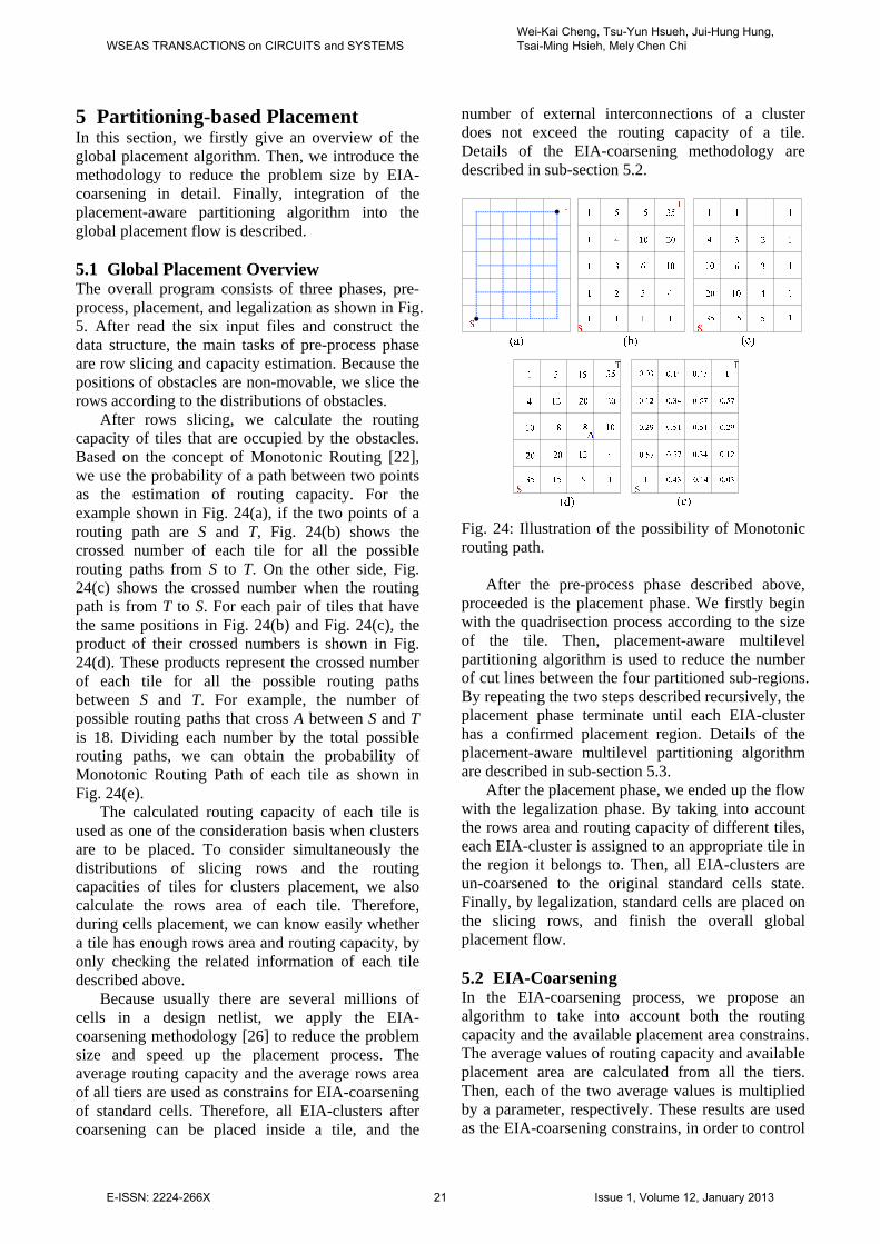
After rows slicing, we calculate the routing capacity of tiles that are occupied by the obstacles. Based on the concept of Monotonic Routing [22], we use the probability of a path between two points as the estimation of routing capacity. For the example shown in Fig. 24(a), if the two points of a routing path are S and T, Fig. 24(b) shows the crossed number of each tile for all the possible routing paths from S to T. On the other side, Fig. 24(c) shows the crossed number when the routing path is from T to S. For each pair of tiles that have the same positions in Fig. 24(b) and Fig. 24(c), the product of their crossed numbers is shown in Fig. 24(d). These products represent the crossed number of each tile for all the possible routing paths between S and T. For example, the number of possible routing paths that cross A between S and T is 18. Dividing each number by the total possible routing paths, we can obtain the probability of Monotonic Routing Path of each tile as shown in Fig. 24(e).

The calculated routing capacity of each tile is used as one of the consideration basis when clusters are to be placed. To consider simultaneously the distributions of slicing rows and the routing capacities of tiles for clusters placement, we also calculate the rows area of each tile. Therefore, during cells placement, we can know easily whether a tile has enough rows area and routing capacity, by only checking the related information of each tile described above.

Because usually there are several millions of cells in a design netlist, we apply the EIA-coarsening methodology [26] to reduce the problem size and speed up the placement process. The average routing capacity and the average rows area of all tiers are used as constrains for EIA-coarsening of standard cells. Therefore, all EIA-clusters after coarsening can be placed inside a tile, and the

number of external interconnections of a cluster does not exceed the routing capacity of a tile. Details of the EIA-coarsening methodology are described in sub-section 5.2.

Fig. 24: Illustration of the possibility of Monotonic routing path.

After the pre-process phase described above, proceeded is the placement phase. We firstly begin with the quadrisection process according to the size of the tile. Then, placement-aware multilevel partitioning algorithm is used to reduce the number of cut lines between the four partitioned sub-regions. By repeating the two steps described recursively, the placement phase terminate until each EIA-cluster has a confirmed placement region. Details of the placement-aware multilevel partitioning algorithm are described in sub-section 5.3.

After the placement phase, we ended up the flow with the legalization phase. By taking into account the rows area and routing capacity of different tiles, each EIA-cluster is assigned to an appropriate tile in the region it belongs to. Then, all EIA-clusters are un-coarsened to the original standard cells state. Finally, by legalization, standard cells are placed on the slicing rows, and finish the overall global placement flow. 5.2 EIA-Coarsening In the EIA-coarsening process, we propose an algorithm to take into account both the routing capacity and the available placement area constrains. The average values of routing capacity and available placement area are calculated from all the tiers. Then, each of the two average values is multiplied by a parameter, respectively. These results are used as the EIA-coarsening constrains, in order to control



A20

B60

C30

D50

External Net

Internal Net

the number of external connections and area of each cluster.

Illustration of the EIA-coarsening algorithm is described as below. All nets are partitioned into two-pin nets firstly. Then for any two cells, their connection information is analyzed when they are coarsened into a cluster. For the example in Fig. 25, when cell A and cell B are coarsened into a cluster, there are totally two external nets and one internal net, and the cluster area is 80. This means that this cluster can be placed into a tier that its available placement area is greater than 80, and will occupy at least two routing capacity of the tier. Fig. 25: Illustration of EIA-coarsening.

Because only the external nets between tiers are considered in the global routing stage as shown in Fig. 26, the more the internal nets inside the tiers, the less the routing wires required for the global router. Therefore, selection of candidates for EIA-coarsening are based on the rules that having less external nets, more internal nets, and smaller cluster area. And the cluster after coarsening must not violate the EIA-coarsening constrains described above.

Fig. 26: Illustration of internal and external routing demands. 5.3 Placement-aware Multilevel Partitioning Each time after the target region is partitioned into four sub-regions by the quadrisection methodology, we calculate the available placement area of each sub-region, and use it as the area constraint of the placement-aware partitioning algorithm. The upper-

bound and lower-bound areas for each sub-region are described in Equation (1), Equation (2) and Equation (3), such that after placement-aware partitioning, areas of each sub-region are close to equally equivalent, to prevent too many cells be distributed in one sub-region.

Aratio_i = AtotalCells × (Auseable_i / AtotalUseable) (1) Aupperbound_i = Aratio_i × rupper (2) Alowerbound_i = Aratio_i × rlower (3)

In Equation (1), Auseable_i is notation for useable area of the ith sub-region; AtotalCells and AtotalUseable are notations for total cell areas and total useable areas of the target region, respectively. In Equation (2) and Equation (3), Aupperbound_i and Alowerbound_i are notations for upper-bound and lower-bound areas of the ith sub-region, respectively; rupper and rlower are user defined parameters to represent the area ratios of upper-bound and lower-bound, respectively.

After calculation of the area bounds, we use the best-choice methodology [20] to do the coarsening for the four sub-regions. Then, we use the quadratic placement methodology [21] to get the initial distribution solution of coarsening clusters in the four sub-regions. Finally, we apply the placement-aware partitioning algorithm proposed in section 4, and followed by clusters un-coarsening to minimize the number of cut lines between sub-regions. The flow of the placement-aware multilevel partitioning is shown in Fig. 27.

Fig. 27: Program flow of the placement-aware multilevel partitioning algorithm.

6 Experimental Results We implement the proposed algorithms by the C/C++ programming language. The platform is Linux system running on the 2.0GHz Intel Xeon E5335 CPU with 16GB RAMs. Four benchmarks



from the 2011 ISPD contest [3] are used to test the performance of our approach. Table 1 lists the characteristics of the four benchmark circuits. Among these characteristics, the column “Total Nodes” lists the total number of standard cells and obstacles, while the column “Movable Nodes” lists the number of standard cells only.

Table 1: Characteristics of the benchmarks.

Benchmarks Total Nodes Movable Nodes

Total Nets Total Pins

superblue4 600,220 521,466 567,607 1,884,008

superblue12 1,293,433 1,278,084 1,293,436 4,774,069

superblue15 1,123,963 829,614 1,080,409 3,816,680

superblue18 483,452 442,405 468,918 1,864,306

We apply the proposed placement-aware

partitioning algorithm to the practical placement problem, and compare our results with both the algorithm proposed by [13], and when no terminal propagation is applied. We firstly compare the results in terms of the half perimeter wire length (HPWL). As shown in Table 2, we got the best results for all the four benchmarks. In comparison with the results without applying the terminal propagation methodology, our results reduced the wire length by 37% in average. Even in comparison with the terminal propagation methodology proposed by [13], our algorithm reduced the wire length by 10% in average.

In addition, we also compare the results after placement in terms of the Steiner tree wire length (STWL) proposed by the FLUTE [23][24][25] algorithm. As shown in Table 3, we got the best results for all the four benchmarks. Our results reduced the wire length by 31% in average when comparing with the results without applying the terminal propagation methodology. And our algorithm also reduced the wire length by 9% in average in comparison with the terminal propagation methodology proposed by [13].

Finally, we compare the results after global routing in terms of wire length and routability. After partitioning and placement, global routing was accomplished with the golden router provided by the 2011 ISPD contest [3]. In Table 4, the column “WL” lists the real wire length after global routing. Comparison results show that with the proposed terminal propagation algorithm, the reduction of real wire length after global routing is even larger than that estimated by HPWL or STWL after placement. In average, we can reduce the total wire length by 55% and 36% in comparison with no terminal

propagation applied and the algorithm proposed by [13], respectively.

In Table 5, we show that except the reduction of total wire length, our placement-aware partitioning algorithm also got better results in terms of routability. The column “Total Overflow” denotes the number of routing wires that exceed the constrained routing capacity. In average, we can reduce the total overflow of routing wires by 253% and 171%, respectively, in comparison with the methodologies described as before.

7 Conclusion In this paper, we propose a placement-aware partitioning algorithm. Based on the terminal propagation rules, and inserting of dummy cells in adequate sub-regions, our placement-aware FM algorithm take into account the interconnections with external pins effectively, and calculate the change of cut lines accurately when cells are moved to other sub-regions. Furthermore, with the application of successive 2-way partitioning instead of k-way partitioning, we get the better partition results and speedup the calculation of gain value simultaneously. Experimental results show that our methodology reduces the total wire length after placement in terms of both HPWL and STWL, and also reduces the total length of routing wires after global routing. Even not considering the routability issue in our algorithm, experimental results show that we also get a not bad solution in terms of this issue. References: [1] 2011 CAD Contest Website:

http://cad_contest.cs.nctu.edu.tw/cad11/Problems.htm

[2] Industrial Technology Research Institute (ITRI), Hsinchu, Taiwan, 2011.

[3] 2011 ISPD Contest Website: http://www.ispd.cc/contests/11/ispd2011_contest.html

[4] G. Karypis, R. Aggarwal, V. Kumar, and S. Shekhar, “Multilevel Hypergraph Partitioning: Application in VLSI Domain”, Proc of. Design Automation Conf., pp. 526-529, 1997.

[5] G. Karypis, V. Kumar, “Multilevel k-way Hypergraph Partitioning”, Proc. of Design Automation Conf., pp. 343-348, 1999.

[6] G. Karypis, R. Aggarwal, V. Kumar, and S. Shekhar, “Multilevel Hypergraph Partitioning: Applications in VLSI Domain”, IEEE Transactions on VLSI System., pp. 69-79, March 1999.



[7] C. M. Fiduccia and R. M. Mattheyses, “A Linear Time Heuristic for Improving Network Partitions”, Proc. of Design Automation Conf, pp. 175-181, 1982.

[8] Iris H. R. Jiang, “Generic Integer Linear Programming Formulation for 3D IC Partition”, proc. of International SOC Conference, pp. 321-324, 2009.

[9] H. S. Ye, M. C. Chi, S. H. Huang, “A Design Partitioning Algorithm for Three Dimensional Integrated Circuits”, proc. of International Sym. on Computer, Communication, Control and Automation, pp. 229-232, 2010.

[10] Y. C. Hu, Y. L. Chung and Mely Chen Chi, “A Multilevel Multilayer Partitioning Algorithm for Three Dimensional Integrated Circuit”, proc. of International Sym. on Quality Electronic Design, pp. 483-487, 2011.

[11] T. Y. Hsueh, H. H. Yang, W. C. Wu and M. C. Chi, “A Layer Prediction Method for Minimum Cost Three Dimensional Integrated Circuits”, proc. of International Sym. on Quality Electronic Design, pp. 359-363, 2011.

[12] C. C. Chan, Y. T. Yu, Iris H. R. Jiang, “3DICE: 3D IC Cost Evaluation Based on Fast Tier Number Estimation”, proc. of International Sym. on Quality Electronic Design, pp. 50-55, 2011.

[13] A. E. Dunlop and B. W. Kernighan, “A Procedure for Placement of Standard-Cell VLSI Circuits“, IEEE Transactions on Computer-Aided Design of Integrated Circuits and Systems, pp. 92-98, January 1985.

[14] P. R. Suaris and G. Kedem, “Quadrisection: A New Approach to Standard Cell Layout”, Proc. of International Conf. on Computer-Aided Design, pp. 474-477, 1987.

[15] P. R. Suaris and G. Kedem, “Standard Cell Placement by Quadrisection”, Proc. International Conf. Computer Design, pp. 612-615, 1987.

[16] P. R. Suaris and G. Kedem, “An Algorithm for Quadrisection and Its Application to Standard Cell Placement”, IEEE Transactions on Circuits and Systems, pp. 294-303, March 1988.

[17] P. R. Suaris and G. Kedem, “A Quadrisection-based Combined Place and Route Scheme for Standard Cells”, IEEE Transactions on

Computer-Aided Design of Integrated Circuits and Systems, pp. 234-244, March 1989.

[18] D. J.-H Huang and A. B. Kahng, “Partitioning-based Standard-Cell Global Placement with an Exact Objective”, Proc. of International Symposium on Physical Design, pp. 18-25, 1997.

[19] M. Wang, X. Yang, M. Sarrafzadeh, “Draagon2000: Standard-Cell Placement Tool for Large Industry Circuits”, Proc. of International Conf. on Computer Aided Design, November 2000.

[20] C. Alpert, A. Kahng, G.-J. Nam, S. Reda and P. Villarrubia, “A Semi-Persistent Clustering Technique for VLSI Circuit Placement”, Proc. of International Symposium on Physical Design, pp. 200–207, 2005.

[21] J.M. Kleinhans, G. Sigl, F.M. Johannes, and K.J. Antreich, “GORDIAN: VLSI Placement by Quadratic Programming and Slicing Optimization”, IEEE Transactions on Computer-Aided Design of Integrated Circuits and Systems, pp. 356–365, March 1991.

[22] M. Pan, and C. Chu, “FastRoute 2.0: A High-Quality and Efficient Global Router”, Proc. of Asia and South Pacific Design Automation Conf., Jan 2007.

[23] C. Chu, “FLUTE: Fast Lookup Table based Wirelength Estimation Technique”, Proc. of International Conf. on Computer-Aided Design, pp. 696-701, Nov 2004.

[24] C. Chu and Y.-C. Wong, “Fast and Accurate Rectilinear Steiner Minimal Tree Algorithm for VLSI Design”, Proc. of International Symposium on Physical Design, pp. 28–35, 2005.

[25] C. Chu and Y.-C. Wong, “FLUTE: Fast Lookup Table Based Rectilinear Steiner Minimal Tree Algorithm for VLSI Design”, IEEE Transactions on Computer-Aided Design of Integrated Circuits and Systems, pp. 70–93, January 2008.

[26] H. L. Chang, H. C. Lai, T. Y. Hsueh, W. K. Cheng, and M. C. Chi, “A 3D IC Designs Partitioning Algorithm with Power Consideration”, proc. of International Sym. on Quality Electronic Design, 2012.



Table 2: Comparison results in terms of HPWL wire length.

Benchmarks HPWL Comparison

w/o terminal propagation

w/ terminal propagation [13]

Our Approachw/o terminal propagation


Our Approach

superblue4 533,397,258 491,453,656 397,118,197 1.34 1.24 1

superblue12 751,735,720 557,823,757 547,491,443 1.37 1.02 1

superblue15 715,813,952 601,325,516 565,873,400 1.26 1.06 1

superblue18 446,034,423 316,697,473 297,479,479 1.50 1.06 1

Average HPWL Comparison 1.37 1.10 1

Table 3: Comparison results in terms of STWL wire length.

Benchmarks STWL Comparison





Our Approach

superblue4 559,121,149 527,677,383 429,926,185 1.30 1.23 1

superblue12 832,542,837 643,029,216 634,964,894 1.31 1.01 1

superblue15 775,322,845 671,182,923 622,473,475 1.25 1.08 1

superblue18 509,068,939 394,314,878 372,064,298 1.37 1.06 1

Average STWL Comparison 1.31 1.09 1

Table 4: Comparison results in terms of wire length after golden router.

Benchmarks WL Comparison





Our Approach

superblue4 24,100,489 22,253,291 16,384,100 1.47 1.36 1

superblue12 42,414,522 38,469,783 25,447,600 1.67 1.51 1

superblue15 37,873,901 32,471,936 24,875,200 1.52 1.31 1

superblue18 23,085,690 18,757,560 14,813,100 1.56 1.27 1

Average WL Comparison 1.55 1.36 1

Table 5: Comparison results in terms of total overflow after golden router.

Benchmarks Total Overflow Comparison





Our Approach

superblue4 11,562,246 9,084,720 2,437,986 4.74 3.73 1

superblue12 17,278,800 18,075,300 7,157,350 2.41 2.53 1

superblue15 19,976,400 14,120,372 5,893,128 3.39 2.40 1

superblue18 10,467,588 6,385,006 2,928,582 3.57 2.18 1

Average Total Overflow Comparison 3.53 2.71 1



a methodology for placement-aware partitioning · effectively in order to reduce the design...

Documents