a model-based investigation of soil moisture ... · august 2002 schlosser and milly 483 q 2002...

AUGUST 2002 483S C H L O S S E R A N D M I L L Y

q 2002 American Meteorological Society

A Model-Based Investigation of Soil Moisture Predictability andAssociated Climate Predictability

C. ADAM SCHLOSSER

Center for Ocean–Land–Atmosphere Studies, Calverton, Maryland

P. C. D. MILLY

U. S. Geological Survey, NOAA/Geophysical Fluid Dynamics Laboratory, Princeton, New Jersey

(Manuscript received 18 July 2001, in final form 14 March 2002)

ABSTRACT

Soil moisture predictability and the associated predictability of continental climate are explored as an initial-value problem, using a coupled land–atmosphere model with prescribed ocean surface temperatures. Ensemblesimulations are designed to assess the extent to which initial soil moisture fields explain variance of futurepredictands (soil moisture, near-surface air temperature, and precipitation). For soil moisture, the decrease ofexplained variance with lead time can be characterized as a first-order decay process, and a predictability timescaleis introduced as the lead time at which this decay reaches e21. The predictability timescale ranges from about2 weeks or less (in midlatitudes during summer, and in the Tropics and subtropics) to 2–6 months (in mid- tohigh latitudes for simulations that start in late fall and early winter). The predictability timescale of the modeledsoil moisture is directly related to the soil moisture’s autocorrelation timescale. The degree of translation of soilmoisture predictability to predictability of any atmospheric variable can be characterized by the ratio of thefraction of explained variance of the atmospheric variable to the fraction of explained soil moisture variance.By this measure, regions with the highest associated predictability of 30-day-mean near-surface air temperature(ratio greater than 0.5) are, generally speaking, coincident with regions and seasons of the smallest soil moisturepredictability timescales. High associated temperature predictability is found where strong variability of soilmoisture stress on evapotranspiration and abundant net radiation at the continental surface coincide. The as-sociated predictability of 30-day-mean precipitation, in contrast, is very low.

1. Introduction

Since the pioneering work on atmospheric predict-ability (Lorenz 1965; Charney et al. 1966; Smagorinsky1969), a wealth of numerical and observational studieshave aimed to identify mechanisms of forced variabilityand, hence, sources of potential predictability for a cli-mate system that is inherently chaotic. At the forefrontof this research, studies have demonstrated that knowl-edge of slowly varying sea surface temperatures (SSTs)can enhance our ability to provide skillful monthly-to-seasonal atmospheric predictions (e.g., Lau 1990; Sternand Miyakoda 1995), and that the strongest interannualmodes of SST variability, such as those associated withthe El Nino–Southern Oscillation, are found to be skill-fully predictable out to a 1-yr lead time (e.g., Shukla1998). Additionally, a growing body of evidence indi-cates that slowly varying land surface conditions, inparticular anomalies of continental water storage, have

Corresponding authors address: C. Adam Schlosser, NASA God-dard Space Flight Center, Code 974, Greenbelt, MD 20771.E-mail: [email protected]

a discernible influence on climate variability. The the-oretical and observational basis of the potential role ofsurface–atmosphere interactions on climate anomaliesincludes work as early as that of Namias (1963), andas recent, for example, as that of Durre et al. (2000).Within the past two decades, numerical experimentationhas allowed a more explicit examination of the impactof interactive continental water balance on simulatedatmospheric variability (e.g., Walker and Rowntree1977; Yeh et al. 1984; Gordon and Hunt 1987; Delworthand Manabe 1988; Koster and Suarez 1996, to name afew). In these studies, the impact of modeled soil mois-ture variability and persistence on simulated near-sur-face atmospheric and precipitation variability is dem-onstrated. In addition, the potential for soil moistureinitialization to aid in the accurate simulation of extremeclimate events, such as droughts (e.g., Fennessy andShukla 1999; Atlas et al. 1993; Namias 1991), has beenshown. Overall, studies such as these demonstrate theimpact that soil moisture anomalies can have on sub-sequent atmospheric variability and the persistence ofextreme climate anomalies.

Remote sensing, models, and data assimilation can

484 VOLUME 3J O U R N A L O F H Y D R O M E T E O R O L O G Y

produce estimates of large-scale (i.e., continental toglobal) fields of soil moisture (e.g., Houser et al. 1998;Walker and Houser 2001) potentially suitable for ini-tialization of climate prediction models. However, it re-mains uncertain how useful such estimates would be foroperational climate predictions, as most sensitivity stud-ies have focused on extreme climatic events (e.g., Og-lesby 1991; Atlas et al. 1993). Observational evidence(e.g., Huang and van den Dool 1993) supports the po-tential role of soil moisture information as an opera-tional predictor for continental temperature fluctuations,and modeling (e.g., Dirmeyer 1999; Koster et al. 2000)shows that soil moisture information also has the po-tential to improve seasonal precipitation predictions un-der certain environmental conditions. Nevertheless, twoquestions arise with regard to soil moisture initializationin climate forecasts. First, how can the information beapplied consistently with the definition, framework, andclimatology of soil moisture in the forecast model? Sec-ond, given an optimal application of perfect soil mois-ture information, what is the ultimate increase in pre-dictive skill that we can gain from knowing the initialand subsequently predicted soil moisture for climateforecasts? The first question primarily addresses the op-erational pitfalls that may arise from systematic biasesbetween a coupled model and nature (e.g., Dirmeyer1995; Mitchell et al. 1999). The second question focusesmore on the fundamental limits of predictability of theclimate system. Moreover, insights on the latter questionmight serve as a useful scientific guide toward efficiencyin operational land-data assimilation products. There-fore, efforts should be made, through numerical exper-iments with a variety of climate models, to explicitlyaddress the potential benefits of initial soil moisture in-formation on climate predictability and operational cli-mate prediction.

Herein, we explore the nature of soil moisture pre-dictability and the associated climate predictability fora particular coupled land–atmosphere model using hy-pothetically perfect information on initial soil moisture.We conduct sets of ensemble simulations using a generalcirculation model (GCM) of the atmosphere coupled toan interactive land model that represents the water andenergy balances of the continental surface. In the nextsection, we describe the coupled land–atmosphere GCMused for this study, the ensemble-simulation design, andthe measure of predictability developed for this analysis.In section 3 we present the results of the GCM ensemblesimulations. In addition, a discussion of the factors con-trolling soil moisture and its associated atmospheric pre-dictability is presented. Concluding remarks are givenin section 4.

2. Ensemble simulations

a. Model

Numerical experiments were conducted using theGeophysical Fluid Dynamics Laboratory (GFDL) cli-

mate model, which includes an atmospheric GCM(AGCM) coupled to a simple water- and energy-balancemodel of the continents [similar to that used in Millyand Dunne (1994)]. At the ocean–atmosphere interface,SSTs were prescribed to follow observed geographicand seasonal patterns, with no interannual variability.The GCM contains a dynamical core that solves theequations of motion through the use of spherical har-monics with a rhomboidal-15 (R15) wavenumber trun-cation in the horizontal and nine levels vertically. Grid-based (including land) computations are performed ona 7.58 longitude by 4.58 latitude grid. Daily-average so-lar forcing is specified. Clouds are predicted using asimple relative humidity criterion. Precipitation is cal-culated so as to prevent supersaturation of the air bywater vapor. Vertical convection is treated by moist-convective adjustment of the atmosphere. This GCMhas been shown by Delworth and Manabe (1988) tosimulate the geographical distribution of seasonally(i.e., December–February and June–August) averagedprecipitation and annually averaged runoff reasonablywell against available observations. Moreover, the zon-ally averaged spectra of rainfall (plus snowfall) have aslightly red-noise characteristic. However, shortcomingsdo exist in the model and will be addressed with regardto the findings of this particular study in the concludingsection.

The land parameterization is that described by Man-abe (1969). Soil moisture is tracked in a single store,representing the plant-available water in the plant rootzone. Soil moisture is depleted only by evaporation;runoff occurs only when storage capacity is exceededas a result of infiltration of rainfall and snowmelt. Thesoil moisture (w) balance equation is

dw5 P 2 bE 2 R, (1)pdt

where

wb 5 min , 1 ,[ ]0.75w0

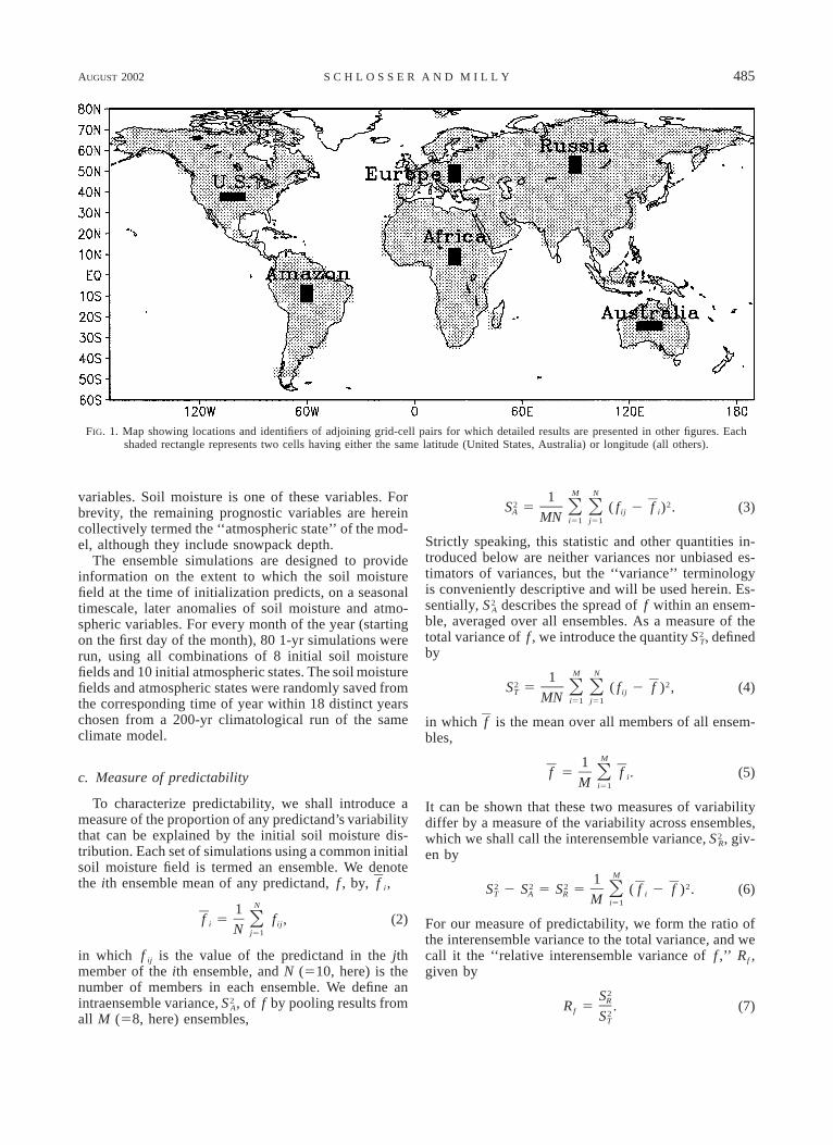
in which w0 is the soil moisture capacity (0.15 m globalconstant), P is the sum of rainfall and snowmelt, Ep isthe potential evaporation rate, and R is runoff, whichoccurs as needed to prevent soil moisture from exceed-ing the capacity. Snowpack is tracked as a separate waterstore. The land has no heat capacity, other than thatassociated with latent heat of fusion of snow. Figure 1shows the representation of the continents by the modelgrid. Also denoted are six selected pairs of adjacent gridcells for which results are highlighted in this paper.

b. Experimental design

Within the climate model, the full state of the climatesystem at any time is described by global, two- andthree-dimensional distributions of several ‘‘prognostic’’


FIG. 1. Map showing locations and identifiers of adjoining grid-cell pairs for which detailed results are presented in other figures. Eachshaded rectangle represents two cells having either the same latitude (United States, Australia) or longitude (all others).

variables. Soil moisture is one of these variables. Forbrevity, the remaining prognostic variables are hereincollectively termed the ‘‘atmospheric state’’ of the mod-el, although they include snowpack depth.

The ensemble simulations are designed to provideinformation on the extent to which the soil moisturefield at the time of initialization predicts, on a seasonaltimescale, later anomalies of soil moisture and atmo-spheric variables. For every month of the year (startingon the first day of the month), 80 1-yr simulations wererun, using all combinations of 8 initial soil moisturefields and 10 initial atmospheric states. The soil moisturefields and atmospheric states were randomly saved fromthe corresponding time of year within 18 distinct yearschosen from a 200-yr climatological run of the sameclimate model.

c. Measure of predictability

To characterize predictability, we shall introduce ameasure of the proportion of any predictand’s variabilitythat can be explained by the initial soil moisture dis-tribution. Each set of simulations using a common initialsoil moisture field is termed an ensemble. We denotethe ith ensemble mean of any predictand, f , by, i,f

N1f 5 f , (2)Oi ijN j51

in which f ij is the value of the predictand in the jthmember of the ith ensemble, and N (510, here) is thenumber of members in each ensemble. We define anintraensemble variance, , of f by pooling results from2S A

all M (58, here) ensembles,

M N12 2S 5 ( f 2 f ) . (3)O OA ij iMN i51 j51

Strictly speaking, this statistic and other quantities in-troduced below are neither variances nor unbiased es-timators of variances, but the ‘‘variance’’ terminologyis conveniently descriptive and will be used herein. Es-sentially, describes the spread of f within an ensem-2S A

ble, averaged over all ensembles. As a measure of thetotal variance of f , we introduce the quantity , defined2S T

byM N1

2 2S 5 ( f 2 f ) , (4)O OT ijMN i51 j51

in which is the mean over all members of all ensem-fbles,

M1f 5 f . (5)O iM i51

It can be shown that these two measures of variabilitydiffer by a measure of the variability across ensembles,which we shall call the interensemble variance, , giv-2S R

en byM1

2 2 2 2S 2 S 5 S 5 ( f 2 f ) . (6)OT A R iM i51

For our measure of predictability, we form the ratio ofthe interensemble variance to the total variance, and wecall it the ‘‘relative interensemble variance of f ,’’ Rf ,given by

2SRR 5 . (7)f 2ST


Note that f and Rf can be defined for any predictedvariable (e.g., soil moisture or atmospheric variable) orfor any time or area average thereof. For any f selectedfor analysis, Rf will be a function of ‘‘lead time’’ (de-fined herein as the time since initialization).

How should we expect Rf to vary with lead time?When f is soil moisture (i.e., Rf [ Rw), all membersof a given ensemble initially have the same value, bydesign, so Rw is initially equal to unity. As lead timeadvances, intraensemble differences in soil moisturewill arise (due to initially different atmospheric states)and grow, causing a decrease in Rw. Sufficiently far intothe future, assuming transitivity of the land–atmospheresystem, separate members of an ensemble can be ex-pected to ‘‘lose the memory’’ of the initial soil moisture.At such lead time, it can be shown that

MN 2 12 2E[S ] → S , (8)T MN

in which S 2 is the variance (in its conventional form)of f in the model. It can also be shown, for large leadtime, that

N 2 12 2E[S ] → S . (9)A N

To a first approximation, it then follows that for any f

M 2 1R → R 5 5 0.089f ` MN 2 1

(for our choice of M and N ). (10)

The timescale of the decay of Rw from unity to this longlead-time value is a measure of the predictability of soilmoisture.

For any atmospheric variable a, Ra is equal to zeroat the start of the simulation period, because all initialatmospheric i are identical by the experimental design.fAt large lead time, Ra will approach the same asymptoticvalue found for soil moisture. Between these two end-points, the behavior of Ra will depend on the extent towhich the atmospheric variable is affected by soil mois-ture. If the atmospheric variable is not sensitive to soilmoisture, then Ra can be expected to rise monotonicallyto its large lead-time value. If, however, soil moisturehas a significant influence on the atmospheric variable,then Ra will initially rise with lead time to a peak higherthan the large lead-time value, to which it will subse-quently decline asymptotically. The timescale of the ini-tial rise is determined by the response rate of the at-mosphere to the underlying land, which we assume tobe faster than the decay rate of Rw to R`. The apex ofthe rise should also be proportional to the sensitivity ofthe atmospheric variable to soil moisture. Furthermore,the timescale of the large lead-time decay of Ra (towardR`) is expected to follow that for soil moisture.

3. Predictability results

a. Soil moisture predictability

Gridpoint samples of Rw time series based on daily(end of day) soil moisture are shown in Fig. 2, usingresults from the simulations initialized in June. The timeseries have the characteristics predicted in the previoussection: they start at unity and decay over lead time toa value that fluctuates around the expected asymptoticvalue. The decay is not regular but can be viewed asthe sum of a smoothly decaying function of lead timeand a random variation. The rate of decay, or charac-teristic timescale of the underlying smooth function,varies from one grid point to the next. In all presentedcases, the decay to the asymptotic value is realized bya lead time of 3 months, but in some cases the decayis much faster. The size of the fluctuations at large leadtime provides a simple index against which the signif-icance of early-time predictability can be subjectivelyassessed.

To characterize the temporal behavior of Rw, we havefitted (via least squares) an exponential decay curve toeach Rw as a function of lead time, t, given by

2t/tWR (t) 5 (1 2 R )e 1 R ,w ` ` (11)

in which R` is the known long lead-time expectationfor Rf [given by Eq. (10)], and tw is a characteristictimescale of soil moisture predictability (i.e., the e-fold-ing timescale of the fitted exponential). Continuous linesin Fig. 2 show fits of Eq. (11) to the data, and Fig. 3(top) shows the superposition of the Rw(t) data fromFig. 2, using a normalized abscissa in time. The ex-ponential function captures the essence of the under-lying temporal decay of Rw(t).

Also shown in Fig. 3 (bottom), for the same samplegrid points, are histories of Rw based on 30-day meansoil moisture. These are constructed by taking f (t) tobe the 30-day running-mean value (in this case, soilmoisture) centered around t, and then calculating Rf asgiven by Eqs. (2)–(7). The resultant quantity is hereafterreferred to as ‘‘30-day Rf ,’’ for any given f . The effectsof using 30-day means instead of daily values aresmoothing of the 30-day Rw(t) curves and slight length-ening of the characteristic timescales. The analysis ofsoil-moisture predictability and atmospheric responsethat follows will be based on the 30-day R results.

The parameter tw is used to characterize the spatialand temporal pattern of soil moisture predictability. Thetime series for 30-day Rw at all land grid points and allinitialization dates were computed and fitted to the ex-ponential-decay model, and, hereafter, the timescale ob-tained from this calculation will be referred to as ‘‘30-day tw.’’ Figure 4 shows how the zonal mean values ofthe estimated 30-day tw depend on month of initiali-zation and latitude. Values of 30-day tw range from lessthan a week in the Tropics to several months for theensembles started during high-latitude fall and winter.Summer values of 30-day tw in the middle and high


FIG. 2. Relative interensemble variance of daily soil moisture, Rw, for the selected grid-cell pairs (of Fig. 1), as afunction of lead time, t (days). Each cell within a pair is denoted by its east/west (E/W) or north/south (N/S) positionwith respect to its counterpart. Results shown are from the simulations starting in June. Also shown are fitted exponentialfunctions (solid curves) associated with tw, and theoretical value of R` (dashed horizontal lines).

latitudes are typically in the range of 2–4 weeks. Mostof the tropical and subtropical regions show relativelylittle seasonal variation and have relatively small 30-day tw values of approximately 1–2 weeks. The zoneof minimum 30-day tw migrates from the northern Trop-ics during Northern Hemisphere summer to the southern

Tropics during northern winter. The long timescales seenin the mid- and high-latitude winter initializations are,in part, contributed by snow cover, which decouples thesoil moisture from the atmosphere in the GFDL GCM;that is, precipitation is not allowed into, nor evaporationfrom, the soil column (and recall there is no gravitational


FIG. 3. Relative interensemble variance of (top) daily soil moisture, Rw and (bottom) 30-daymean soil moisture, 30-day Rw, for the selected grid cells of Fig. 1, as functions of normalizedforecast lead time, t/tw. Distinct values of tw were determined separately for the daily and 30-day results. Results are from the ensemble simulations starting in June. Also shown is the ex-ponential function (heavy solid curve) described by Eq. (11) and the theoretical value of R`

(dashed horizontal line).

drainage in the GFDL bucket formulation). Other con-trols of soil moisture predictability are addressed in sec-tion 4.

Figure 5 shows the global distribution of 30-day tw

for June and December initializations. Because these arebased on results from individual grid points, a signifi-cant amount of random noise is present in these results.Nevertheless, Fig. 5 suggests that global patterns of pre-dictability depart in some regions from what would bepredicted by the zonal-mean patterns already discussedin connection with Fig. 4. In particular, December 30-day tw are somewhat greater than the zonal average incentral North America and in Asia, and less than theaverage in Europe and coastal North America.

b. Associated predictability of near-surface airtemperature

Having reviewed the results for soil moisture pre-dictability, we now examine the resultant predictabilityof near-surface air temperature (T) and precipitation (P).Sample RT(t) data, for daily T, are shown in Fig. 6. Forsome grid points (in particular the Amazon-S and U.S.points), the initial rise of RT from zero at initial time isapparent; for others, the rise is so rapid as to be almostundetectable. At large lead time, RT fluctuates randomlyaround the expected asymptotic value. At most gridpoints, the initial growth from zero leads into an inter-mediate lead-time regime when RT tends to exceed the


FIG. 4. Zonal-mean values (days; land only) of 30-day tw (as defined in the text), as a functionof initialization date of the ensemble simulations and latitude.

asymptotic value. Accordingly, we can infer a certaindegree of T predictability resulting from soil moisturepredictability.

For those grid points in Fig. 6 with a significantinitial rise of RT above its asymptotic value, the time-scale of its decay appears to be on the order of thatof soil moisture predictability. Under our assumptionthat the atmospheric response time is small comparedto 30-day tw (section 2c), it is reasonable to expectthat R of atmospheric variables will decay to R` onthe same timescale as that of soil moisture. As seenin Fig. 6, RT is generally less than Rw for a given leadtime (even after its initial spinup from zero), indi-cating that a given level of soil moisture predictabilitydoes not translate fully to a corresponding level of Tpredictability.

It is reasonable to expect that time averages (low-frequency variations) of atmospheric variables will bemore predictable than daily values (high-frequency var-iations), given that tw is typically on the order of weeks.For this reason, our analysis will focus henceforth on30-day RT (and RP). Figure 7 shows 30-day RT at oursample grid points. In comparison with Fig. 6 for dailyvalues, the 30-day RT values tend to be significantlylarger at the intermediate time when predictability isapparent. In many cases, 30-day RT is nearly equal inmagnitude to the fitted 30-day Rw for a given lead time.Moreover, the expected proportional decay of RT to Rw

at long lead times is much more apparent for the 30-day means as compared to the daily plots (Fig. 6). Thespinup period of 30-day RT is largely absent, due to the

time averaging and that 30-day RT is undefined duringthe first 15 days of the simulation. At long lead times,30-day RT fluctuates around the predicted asymptoticvalue but with considerably greater temporal persistencethan for daily RT. A sensitivity test was performed forthe simulations initialized on 1 June in which the num-ber of ensembles, M, was increased from 8 to 16. Theresults showed considerable reduction in the long lead-time fluctuations while preserving the early lead-timepeaks of 30-day RT. This would suggest that the earlylead-time peaks seen for our set of simulations whereM 5 8 can be viewed as robust.

To escape the apparent noise in gridpoint 30-day RT,we display in Fig. 8 the zonal-mean values of 30-dayRT. Predictability of 30-day mean T is apparent at almostall latitudes, the only exceptions being north of 608Nand south of 308S. For comparison, the corresponding30-day Rw are shown. From 608N to 108S, zonal 30-dayRw and 30-day RT converge within several weeks ofinitialization and decay together thereafter. During theinitial phase before convergence, 30-day Rw exceeds 30-day RT, and we associate this with the initial spinup ofthe atmospheric state. The near-coincidence of the zonal30-day R curves after the time of convergence impliesfull translation of soil moisture predictability to air tem-perature predictability, suggesting near-total control ofnear-surface air temperature anomalies by soil moistureanomalies at the 30-day timescale. This correspondencebreaks down in the Southern (winter) Hemisphere, be-tween 108 and 408S, as the predictability of near-surfaceair temperature decreases progressively to zero, despite


FIG. 5. Global distribution of 30-day tw for ensemble simulations starting (top) 1 Jun and(bottom) 1 Dec.

increasing soil moisture predictability (i.e., larger valuesof 30-day tw).

As Fig. 8 shows, the relation of 30-day Rw to at-mospheric-variable 30-day R can provide a measure ofatmospheric response to a given level of soil moisturepredictability. To formalize this, we introduce the ‘‘as-sociated predictability ratio’’ for any atmospheric var-iable, a, as

R (t) 2 Ra `A 5 . (12)a R (t) 2 Rw `

Note that A cannot be independent of time until afterthe initial atmospheric spinup, and even then only as anapproximation. To allow for the spinup period, we refinethis relation to

R (t) 2 R 5 A [1 2 exp(2t/t )][R (t) 2 R ], (13)a ` a a w `

in which ta is an atmospheric spinup time, reflectingthe timescale of response of the atmosphere from itsinitial state. Using this relation together with the ex-ponential curve to evaluate 30-day Rw, we estimated AT

for all grid points and simulation start dates so as tominimize the squared difference between the two sidesof this equation. For this purpose, we also vary ta, butwe prescribe a maximum value of 2 weeks, which ischaracteristic of a saturation timescale for atmosphericerror growth (cf. Palmer 1993; Simmons et al. 1995;Shukla and Kirtman 1996). Perhaps the most dubiousaspects in estimating our Aa metric [i.e., curve fit of Eq.(13)] are for grid points in which tw , ta, that is, whenthe soil moisture predictability timescale is relativelyshort (typically when tw & 1 week; refer to Fig. 5). Thiswould imply that the soil moisture memory is shorterthan (or comparable to) the spinup timescale from the


FIG. 6. As in Fig. 2, but for relative interensemble variance of daily near-surface air temperature, RT, for ensemblesimulations starting 1 Jun. Also shown for reference are fitted daily Rw curves (solid lines) and theoretical long lead-time value, R` (dashed horizontal lines).

atmospheric initialization. In such cases, associated at-mospheric predictability from soil moisture initializa-tion is intuitively untenable (but from our curve fitsresult in values close to 1), and we therefore prescribeAa 5 0. Figure 8 shows the zonal averages of the fittedcurves for the June initialization of the ensemble sim-

ulations. Because we use both 30-day RT and 30-day Rw

to solve for AT in Eq. (13), we distinguish the diagnosticas ‘‘30-day AT’’ (likewise for our precipitation analysisthat follows).

Figure 9 shows the dependence of zonal-mean 30-day AT on latitude and month of initialization. In the


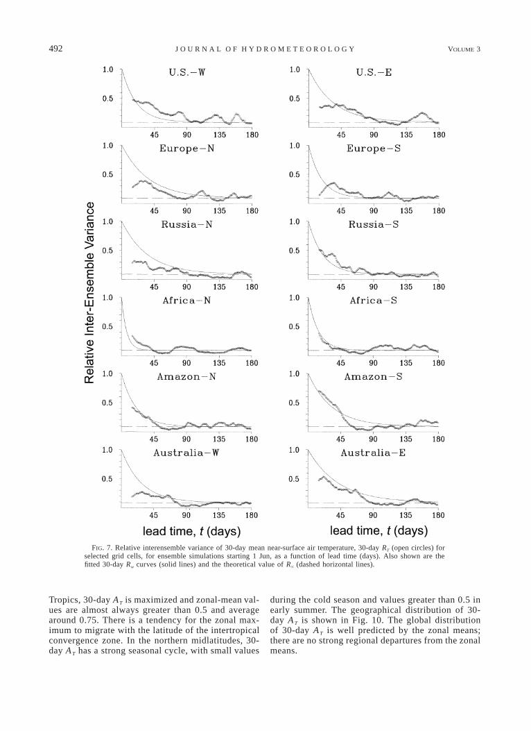
FIG. 7. Relative interensemble variance of 30-day mean near-surface air temperature, 30-day RT (open circles) forselected grid cells, for ensemble simulations starting 1 Jun, as a function of lead time (days). Also shown are thefitted 30-day Rw curves (solid lines) and the theoretical value of R` (dashed horizontal lines).

Tropics, 30-day AT is maximized and zonal-mean val-ues are almost always greater than 0.5 and averagearound 0.75. There is a tendency for the zonal max-imum to migrate with the latitude of the intertropicalconvergence zone. In the northern midlatitudes, 30-day AT has a strong seasonal cycle, with small values

during the cold season and values greater than 0.5 inearly summer. The geographical distribution of 30-day AT is shown in Fig. 10. The global distributionof 30-day AT is well predicted by the zonal means;there are no strong regional departures from the zonalmeans.


FIG. 8. Zonal averages (land only) of relative interensemble variance for 30-day running mean near-surface airtemperature, 30-day RT (open circle), for ensemble simulations starting in June, as functions of lead time (days). Alsoshown are the corresponding data for soil moisture, Rw (cross hair), the zonal mean values of the fitted air temperaturecurve obtained through the curve fit of Eq. (13) (solid line), and the theoretical value of R` (dashed horizontal line).

c. Associated predictability of precipitation

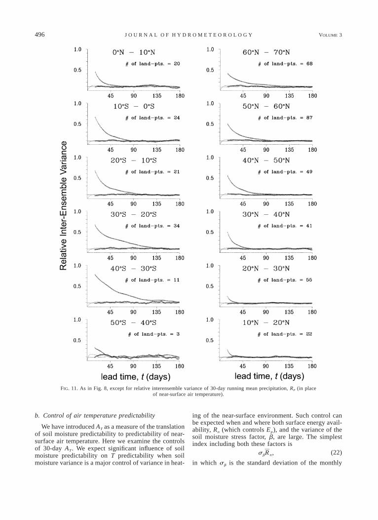
Analysis of our experiments indicated far less asso-ciated predictability for precipitation than for air tem-perature. Figure 11 shows the zonal-mean traces of 30-day RP for June initialization. There are departures of

30-day RP above the asymptotic value that appear to besignificant in some cases, but the magnitude of the pre-dictability is negligibly small. As a result, the values of30-day AP (not shown) that result from the gridpointcurve fitting of (13) reflect an absence of widespreadassociated predictability of precipitation in the model.


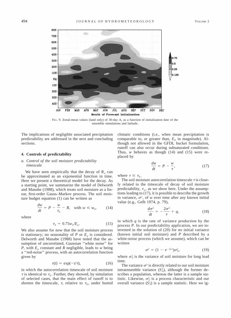
FIG. 9. Zonal-mean values (land only) of 30-day AT as a function of initialization date of theensemble simulations and latitude.

The implications of negligible associated precipitationpredictability are addressed in the next and concludingsections.

4. Controls of predictability

a. Control of the soil moisture predictabilitytimescale

We have seen empirically that the decay of Rw canbe approximated as an exponential function in time.Here we present a theoretical model for the decay. Asa starting point, we summarize the model of Delworthand Manabe (1988), which treats soil moisture as a lin-ear, first-order Gauss–Markov process. The soil mois-ture budget equation (1) can be written as

dw w5 P 2 2 R, with w # w , (14)0dt tE

where

t 5 0.75w /E .E 0 p (15)

We also assume for now that the soil moisture processis stationary; no seasonality of P or Ep is considered.Delworth and Manabe (1988) have noted that the as-sumption of uncorrelated, Gaussian ‘‘white noise’’ forP, with Ep constant and R negligible, leads to w beinga ‘‘red-noise’’ process, with an autocorrelation functiongiven by

r(t) 5 exp(2t/t), (16)

in which the autocorrelation timescale of soil moisturet is identical to tE. Further, they showed, by simulationof selected cases, that the main effect of runoff is toshorten the timescale, t, relative to tE, under humid

climatic conditions (i.e., when mean precipitation iscomparable to, or greater than, EP in magnitude). Al-though not allowed in the GFDL bucket formulation,runoff can also occur during subsaturated conditions.Thus, w behaves as though (14) and (15) were re-placed by

dw w5 P 2 , (17)

dt t

where t # tE.The soil moisture autocorrelation timescale t is close-

ly related to the timescale of decay of soil moisturepredictability, tw, as we show here. Under the assump-tions leading to (17), it is possible to describe the growthin variance, s2, of w over time after any known initialvalue (e.g., Gelb 1974, p. 79),

2 2ds 2s5 2 1 q, (18)

dt t

in which q is the rate of variance production by theprocess P. In our predictability application, we are in-terested in the solution of (20) for no initial variance(known initial soil moisture) and P described by awhite-noise process (which we assume), which can bewritten

2 22t/t 2s 5 (1 2 e )s ,0 (19)

where is the variance of soil moisture for long lead2s 0

time.The variance s2 is directly related to our soil moisture

intraensemble variance ( ), although the former de-2S A

scribes a population, whereas the latter is a sample sta-tistic. Likewise, is a process characteristic and our2s 0

overall variance ( ) is a sample statistic. Here we ig-2S T


FIG. 10. Global distribution of 30-day AT for ensemble simulations starting (top) 1 Jun and(bottom) 1 Dec.

nore these distinctions, which is equivalent to assumingthat M and N are sufficiently large. Then we find, from(6), (7), and (21),

2s22t /tR (t) 5 1 2 5 e . (20)w 2so

Equation (22) explains the empirically determined ex-ponential character of the Rw curves and predicts theirdecay timescale to be half the timescale of the decay ofsoil moisture autocorrelation,

t 5 t/2.w (21)

All of this theory has been developed without con-sideration of seasonal changes in climate. To the extentthat t is much shorter than 1 yr, this theory can beassumed to apply during any particular season of theyear, with Ep being representative of that season. Inseasons for which the t so determined would be several

months or longer, the error of the estimate of t (andtherefore tw) will be a function, in part, by antecedentand subsequent statistics of the seasonality of Ep (or,more generally, the atmospheric forcing) as well as thestrength of land–atmosphere feedbacks (Koster and Sua-rez 2001).

In light of these expected limitations, the utility ofusing (23) to predict tw is demonstrated for the simu-lations initialized in June (Fig. 12). In order to obtainan estimate of t for (23), 7-day lagged autocorrelationsof daily soil moisture are determined from the 200-yrclimatological run (described in section 2). These point-wise autocorrelations are then inserted into (16) andsolved for t (with a value of t 5 7 days). A robustspatial correspondence is found between the predictedand actual values of tw, with the global, spatial corre-lation coefficient significant (50.67, land points only)above the 99% significance level.


FIG. 11. As in Fig. 8, except for relative interensemble variance of 30-day running mean precipitation, RP (in placeof near-surface air temperature).

b. Control of air temperature predictability

We have introduced AT as a measure of the translationof soil moisture predictability to predictability of near-surface air temperature. Here we examine the controlsof 30-day AT. We expect significant influence of soilmoisture predictability on T predictability when soilmoisture variance is a major control of variance in heat-

ing of the near-surface environment. Such control canbe expected when and where both surface energy avail-ability, Rn (which controls Ep), and the variance of thesoil moisture stress factor, b, are large. The simplestindex including both these factors is

s R ,b n (22)

in which sb is the standard deviation of the monthly


FIG. 12. Global distribution of soil moisture predictability timescales, tw. (bottom) Equation(23) is used to obtain a theoretical estimate of tw. To obtain an estimate of t, 7-day laggedautocorrelations from the GCM’s 200-yr climatological run are used to solve Eq. (16) with t 57 days. This estimate is compared to (top) the tw values obtained directly from the GCM ensemblesimulations. Results are shown for the ensemble simulations initialized 1 Jun.

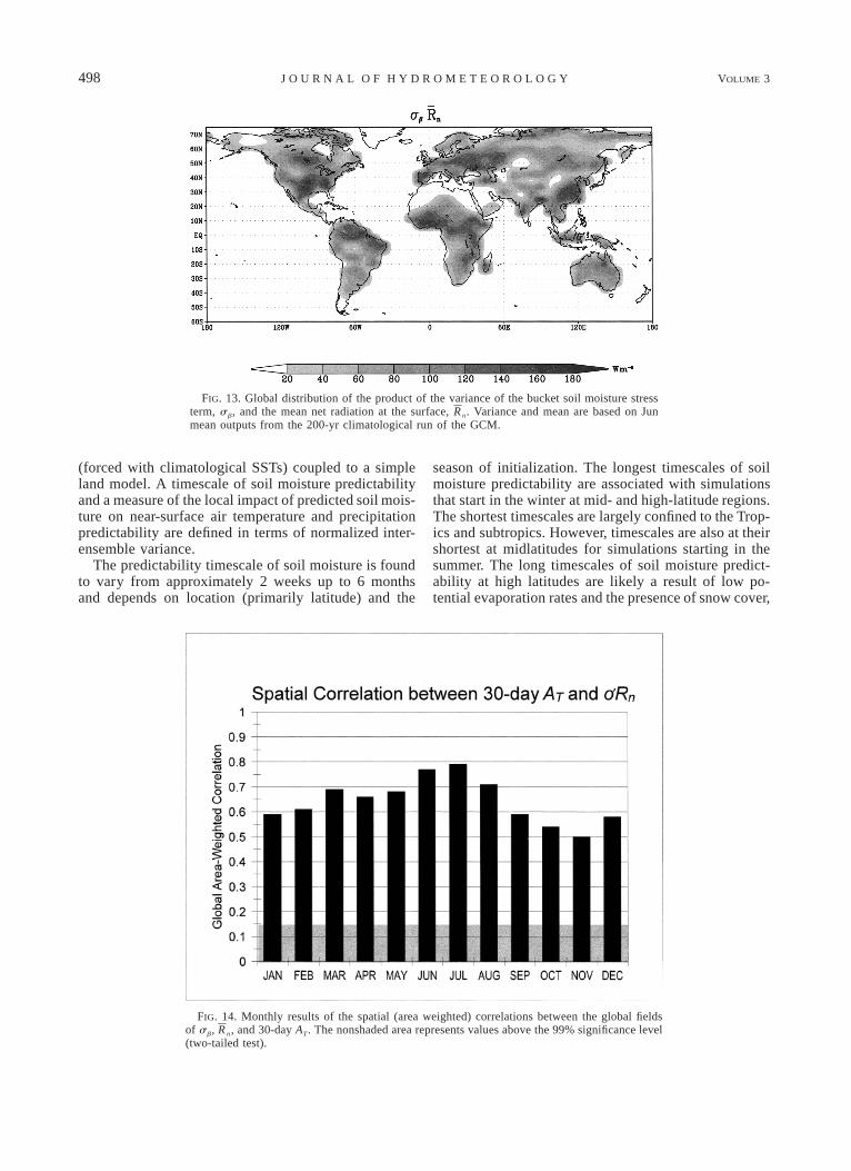
mean soil moisture stress factor and n is monthly meanRnet radiation. Relatively large values of this indexshould reflect an environment that supports strong, localcoupling between soil moisture and turbulent heat-fluxpartitioning, hence T variability, and, therefore, a highvalue of 30-day AT. On the other hand, when (24) issmall, we expect 30-day AT to tend to zero. The abilityof this index to predict 30-day AT is demonstrated forthe simulations initialized for June (Fig. 13). The indexshows a robust (and significant at the 99% level) con-sistency with 30-day AT for June (Fig. 10). Overall, asignificant geographical correspondence between this

index and 30-day AT is seen for all initialization monthsof the ensemble simulations (Fig. 14). However, thiscorrespondence does not necessarily imply causality.

5. Closing remarks

a. Summary

Using a coupled land–atmosphere model, we haveexplored the nature of soil moisture predictability andassociated atmospheric predictability. Sets of ensemblesimulations were performed using the GFDL R15 GCM


FIG. 13. Global distribution of the product of the variance of the bucket soil moisture stressterm, sb, and the mean net radiation at the surface, n. Variance and mean are based on JunRmean outputs from the 200-yr climatological run of the GCM.

FIG. 14. Monthly results of the spatial (area weighted) correlations between the global fieldsof sb, n, and 30-day AT. The nonshaded area represents values above the 99% significance levelR(two-tailed test).

(forced with climatological SSTs) coupled to a simpleland model. A timescale of soil moisture predictabilityand a measure of the local impact of predicted soil mois-ture on near-surface air temperature and precipitationpredictability are defined in terms of normalized inter-ensemble variance.

The predictability timescale of soil moisture is foundto vary from approximately 2 weeks up to 6 monthsand depends on location (primarily latitude) and the

season of initialization. The longest timescales of soilmoisture predictability are associated with simulationsthat start in the winter at mid- and high-latitude regions.The shortest timescales are largely confined to the Trop-ics and subtropics. However, timescales are also at theirshortest at midlatitudes for simulations starting in thesummer. The long timescales of soil moisture predict-ability at high latitudes are likely a result of low po-tential evaporation rates and the presence of snow cover,


which in the GFDL bucket hydrology decouples soilmoisture from the atmosphere.

The associated predictability of near-surface air tem-perature over the land is strongest in the Tropics andthe subtropics. However, a notable impact is also seenin the midlatitudes for simulations initialized in the latespring through summer. The associated predictability ofprecipitation, however, is insensitive, locally, to pre-dicted soil moisture. The geographic locations of great-est associated predictability of near-surface air temper-ature are coincident with locations in which net radiationat the surface is abundant and the temporal variabilityof soil moisture control on surface heat fluxes is high.No substantial associated precipitation predictability ofprecipitation was found.

b. Discussion

The diagnostic results of simulated soil moisture pre-dictability and associated atmospheric predictability are,indeed, model dependent. This study was based on nu-merical experimentation using the GFDL AGCM cou-pled to a simple land model. The theoretical relationship(presented in section 3) between soil moisture persis-tence and predictability timescales [Eq. (23)] was builtupon the GFDL land model’s linear relation betweensoil moisture and its stress on evapotranspiration(among other simplifying assumptions), which allowsthe soil moisture budget equation to be viewed as alinear Markov process. More complex (i.e., nonlinear)relations between soil moisture and its stress on evapo-transpiration exist in most land models that are used forcomputational climate research [for reviews see Shaoand Henderson-Sellers (1996) and Mahfouf et al.1996)]. As such, the relation between soil moisture pre-dictability and persistence presented in this work is notguaranteed to apply as a general rule. However, a recentstudy by Koster and Milly (1997) shows that the annualcycle of the water budgets of more complex land modelscan be captured through linear approximations (as afunction of soil moisture) of their evaporation and runoffformulations. Therefore, it is reasonable to expect that,to a certain extent, the relation between soil moisturepredictability and persistence in most land models canbe approximated through a linear, Markovian frame-work. Perhaps more compelling, the results of Vinnikovand Yeserkepova (1991) using gravimetric soil moistureobservations (for primarily grassland plots) over the for-mer Soviet Union empirically support the Markovianbehavior of soil moisture persistence and, therefore, byextension of our analysis, its predictability. Therefore,while the limited scope (both in space and bio-geolog-ical extent) of their observations precludes any generalconclusions in this regard, it warrants further studies todo so.

A similar consideration of our theory relating soilmoisture predictability and persistence should be madewith regard to nonlinear and nonlocal interactions be-

tween soil moisture and precipitation (as well as a re-mote SST influence on precipitation, which is addressedin a subsequent paragraph). Note that for the limitingcase of a local, linear interaction between soil moistureand precipitation, a linear damping term similar to thatused for evapotranspiration stress (i.e., the b term) canbe included in the soil moisture budget equation [Eqs.(14) and (17)] to represent the local response of pre-cipitation to soil moisture. Therefore, the essence of thelinear Markov process for soil moisture is retained.However, a nonlocal and/or nonlinear impact of soilmoisture on precipitation cannot be conveniently de-scribed within the context of a linear Markov represen-tation of the soil moisture budget. Nevertheless, anypersistence of precipitation induced by nonlinear and/or nonlocal feedbacks will, in turn, enhance soil mois-ture persistence and predictability [beyond what wouldbe estimated by Eq. (23)]. In this case, our theoreticalmodel of the soil moisture predictability timescale couldbe viewed as an underestimate. The results of recentnumerical experiments (Koster et al. 2002) show a widerange of strength in land–atmosphere coupling (in par-ticular, the response of precipitation to land surfaceevaporation efficiency) for four particular GCMs. Theprecipitation processes that are parameterized, the land–atmosphere coupling strategies employed, (Polcher etal. 1998) as well as the degree to which near-surfaceatmospheric profiles are adequately resolved (K. Findell2002, personal communication) likely contribute to themodel scatter and the accuracy of any model result.These issues further underscore the sensitivity of thenumerical representation of coupled-climate processeson their coupled modes of predictability. Nevertheless,the low AP found in our analysis [qualitatively consistentwith three of the four GCMs’ results in Koster et al.(2002)] is indicative of a weak, local soil moisture–precipitation interaction in the GFDL GCM. Therefore,our theoretical model [Eq. (23)] is able to predict thesoil moisture predictability timescales reasonably well(Fig. 12), because the theory leading to Eq. (23) is basedupon an assumption (among others) that precipitationis a white-noise process (i.e., no land–atmosphere feed-backs occur).

Our relation between soil moisture persistence andpredictability further emphasizes the crucial role accu-rate soil moisture modeling plays in climate prediction;if a particular land model exhibits spurious modes ofsoil moisture persistence (due to inaccurate parameter-izations), this will likely lead to spurious modes of soilmoisture predictability (and associated atmospheric pre-dictability). As such, future efforts should be made toevaluate simulated soil moisture persistence of currentland models over large scales (continental to global) atresolutions consistent with AGCMs. Current efforts torun land models at the global scale over many years(Polcher 2000), as well as the collection of in situ (e.g.,Entin et al. 2000) and remote sensing data (e.g., Walker


and Houser 2001) to monitor and analyze soil moistureglobally, will prove valuable in this regard.

Delworth and Manabe (1988) showed some rednessand, hence, some (implied) associated predictability ofspatially filtered (i.e., nine-point smoothed) precipita-tion in the GFDL AGCM. The results presented hereindicate that the local impact of soil moisture variabilityon subsequent precipitation is weak. The apparent dis-parity between these findings has been addressed bycalculating our R and Aa diagnostics on spatially filtered(i.e., five-point smoothed) soil moisture and precipita-tion fields. These complementary diagnostics were con-ducted for the forecasts starting 1 June and indicate thatspatially filtered values of precipitation lead to small,but discernible, peaks of 30-day RP that rise above R`

at early lead times (unlike the flat curves of zonallyaveraged 30-day RP shown in Fig. 11). This would in-dicate that spatial filtering of 30-day mean precipitationcould lead to more robust results for the AP diagnostics,but only marginally so. Overall, the results indicate apotential enhancing effect of spatial and temporal av-eraging on these types of explained-variance/predict-ability diagnostics.

Looking further at the results of Delworth and Man-abe (1989), we see a strong impact of soil moisturevariability on the power spectrum of near-surface rel-ative humidity index (a reddening effect). Koster et al.(2000) present an intuitive basis for the conditions inwhich a strong coupling between land surface and pre-cipitation variability would be expected. They argue(and support through experimental results from theirparticular GCM) that regions of intermediate near-sur-face relative humidity (and where the spatial gradientsof relative humidity are strong) would be most con-ducive to a strong land surface–precipitation interaction.The results of this study would indicate that, althougha strong coupling between soil moisture and near-sur-face relative humidity exists in the GFDL GCM, thisdoes not translate into widespread precipitation pre-dictability. This disparity could be a result of the factthat the apparent near-surface humidity control in theGFDL GCM is largely a manifestation of soil moisture’scontrol on near-surface temperature variability (sup-ported by the strong AT results) rather than a moistureflux effect (via surface evaporation).

These predictability experiments were conducted us-ing climatological SSTs as boundary conditions. There-fore, any influence of ocean variability on these pre-dictability results was removed. In light of the wealthof numerical studies that have studied the impact of theocean on atmospheric variability and predictability (e.g.,see section 1), it is reasonable to assume that includingknowledge of interannual SST variations in these ex-periments would cause an appreciable (and predictable)response of the atmosphere (i.e., a precipitation anom-aly). Over the continents, any predictable precipitationresponse could result in a predictable soil moistureanomaly. While this may lead to enhanced predictability

of soil moisture (and the atmosphere), it is the result ofan atmospheric response to the ocean, rather than theresponse to initial soil moisture information. Our intentfor these experiments was to obtain the predictabilitysignal that results solely from the knowledge of initialsoil moisture, and therefore we have removed the oceaninfluence.

Nevertheless, the results presented indicate that initialsoil moisture information would have a widespread, pre-dictable effect on climate predictions with the GFDLGCM for monthly soil moisture and near-surface airtemperature, especially for the Tropics and subtropics,and for forecasts starting in the summer at midlatitudes.Many previous GCM experiments have investigated theimpact of soil moisture initialization on simulating ex-treme climate events (e.g., Atlas et al. 1993) and in somecases used idealized and/or extreme values for their soilmoisture initialization (e.g., Oglesby 1991). Studies likethese are useful for ascertaining the role of land–at-mosphere interactions under extreme conditions butcannot quantify whether these events are predictable, orwhether soil moisture can provide a useful predictiveimpact for climate simulations under less extreme cli-mate conditions. The global soil moisture fields used toinitialize the ensemble simulations were essentially tak-en at random from a climatological run of the GFDLGCM. Therefore, a wide range of soil moisture con-ditions (i.e., from wet to dry regions) is represented. Assuch, our analysis reflects a broader perspective of theimpact of soil moisture initialization on soil moisturepredictability and its subsequent predictable impact incoupled climate simulations.

Acknowledgments. We wish to thank Syukuro Man-abe, Tom Delworth, Timothy DelSole, and Jeffery An-derson for valuable discussions and insights during thecourse of this study. We thank Randy Koster, Paul Dir-meyer, Kirsten Findell, and two anonymous reviewersfor constructive and insightful comments. We wouldalso like to thank Krista Dunne for providing her tech-nical expertise during the construction of the numericalexperiments. All figures except Fig. 14 were plottedusing the GrADS software developed by Brian Doty.

REFERENCES

Atlas, R., N. Wolfson, and J. Terry, 1993: The effect of SST and soilmoisture anomalies on GLA model simulations of the 1988 U.S.summer drought. J. Climate, 6, 2034–2048.

Charney, J. G., R. G. Fleagle, H. Riehl, V. E. Lally, and D. Wark,1966: The feasibility of a global observation and analysis ex-periment. Bull. Amer. Meteor. Soc., 47, 200–220.

Delworth, T. D., and S. Manabe, 1988: The influence of potentialevaporation on the variabilities of simulated soil wetness andclimate, J. Climate, 1, 523–547.

——, and ——, 1989: The influence of soil wetness on near-surfaceatmospheric variability. J. Climate, 2, 1449–1462.

——, and ——, 1993: Climate variability and land-surface processes.Adv. Water Res., 16, 3–20.


Dirmeyer, P. A., 1995: Problems in initializing soil wetness. Bull.Amer. Meteor. Soc., 76, 2234–2240.

——, 1999: Assessing GCM sensitivity to soil wetness using GSWPdata. J. Meteor. Soc. Japan, 77, 367–384.

Durre, I., J. M. Wallace, and D. P. Lettenmaier, 2000: Dependenceof extreme daily maximum temperatures on antecedent soil mois-ture in the contiguous United States during summer. J. Climate,13, 2641–2651.

Entin, J., A. Robock, K. Ya. Vinnikov, S. E. Hollinger, S. Liu, andA. Namkhai, 2000: Temporal and spatial scales of observed soilmoisture variations in the extratropics. J. Geophys. Res., 105,11 865–11 878.

Fennessy, M., and J. Shukla, 1999: Impact of initial soil wetness onseasonal atmospheric prediction. J. Climate, 12, 3167–3180.

Gelb, A., Ed.,1974: Applied Optimal Estimation. MIT Press, 374 pp.Gordon, H. B., and B. G. Hunt, 1987: Interannual variability of the

simulated hydrology in a climatic model—Implications fordrought. Climate Dyn., 1, 113–130.

Houser, P. R., W. J. Shuttleworth, J. S. Famiglietti, H. V. Gupta, K.H. Syed, and D. C. Goodrich, 1998: Integration of soil moistureremote sensing and hydrologic modeling using data assimilation.Water Resour. Res., 34, 3405–3420.

Huang, J., and H. M. van den Dool, 1993: Monthly precipitation–temperature relations and temperature prediction over the UnitedStates. J. Climate, 6, 1350–1362.

Koster, R. D., and M. J. Suarez, 1996: The influence of land surfacemoisture retention on precipitation statistics. J. Climate, 9, 2551–2567.

——, and P. C. D. Milly, 1997: The interplay between transpirationand runoff formulations in land surface schemes used with at-mospheric models. J. Climate, 10, 1578–1591.

——, and M. J. Suarez, 2001: Soil moisture memory in climate mod-els. J. Hydrometeor., 2, 558–570.

——, ——, and M. Heiser, 2000: Variance and predictability of pre-cipitation at seasonal-to-interannual timescales. J. Hydrometeor.,1, 26–46.

——, P. A. Dirmeyer, A. N. Hahmann, R. Ijpelaar, L. Tyahla, P. Cox,and M. J. Suarez, 2002: Comparing the degree of land–atmo-sphere interaction in four atmospheric general circulation mod-els. J. Hydrometeor., 3, 363–375.

Lau, N.-C., and M. J. Nath, 1990: A general circulation model studyof the atmospheric response to extratropical SST anomalies ob-served in 1950–1979. J. Climate, 3, 965–989.

Lorenz, E. N., 1965: A study of the predictability of a 28-variableatmospheric model. Tellus, 17, 321–333.

Mahfouf, J.-F., and Coauthors, 1996: Analysis of transpiration resultsfrom the RICE and PILPS Workshop. Global Planet. Change,13, 73–88.

Manabe, S., 1969: Climate and ocean circulation. Part I: The at-mospheric circulation and the hydrology of the earth’s surface.Mon. Wea. Rev., 97, 739–774.

Milly, P. C. D., and K. Dunne, 1994: Sensitivity of the global water

cycle to the water-holding capacity of land. J. Climate, 7, 506–526.

Mitchell, K., and Coauthors, 1999: The collaborative GCIP Land DataAssimilation (LDAS) project and supportive NCEP uncoupledland-surface modeling initiatives. Preprints, 15th Conf. on Hy-drology, Long Beach, CA, Amer. Meteor. Soc., 1–4.

Namias, J., 1963: Surface–atmosphere interactions as fundamentalcauses of droughts and other climatic fluctuations. Arid ZoneResearch, Vol. 20, Changes of Climate: Proc. of Rome Sym-posium, Rome, Italy, UNESCO, 345–359.

——, 1991: Spring and summer 1988 drought over the contiguousUnited States—Causes and prediction. J. Climate, 4, 54–65.

Oglesby, R. J., 1991: Springtime soil moisture, natural climate var-iability, and North American drought as simulated by the NCARCommunity Climate Model I. J. Climate, 4, 890–897.

Palmer, T. N., 1993: Extended-range atmospheric prediction and theLorenz model. Bull. Amer. Meteor. Soc., 74, 49–65.

Polcher, J., 2000: GLASS implementation underway. GEWEX News,10 (4), 9.

——, and Coauthors, 1998: A proposal for a general interface be-tween land surface schemes and general circulation models.Global Planet. Change, 19, 261–276.

Press, W. R., B. P. Flannery, S. A. Teulosky, and W. T. Vetterling,1986: Numerical Recipes: The Art of Scientific Computing. Cam-bridge University Press, 702 pp.

Shao, Y., and A. Henderson-Sellers, 1996: Validation of soil moisturesimulation in land surface parameterization schemes with HAP-EX data. Global Planet. Change, 13, 11–46.

Shukla, J., 1998: Predictability in the midst of chaos: A scientificbasis for climate forecasting. Science, 282, 728–731.

——, and B. Kirtman, 1996: Predictability and error growth in acoupled ocean–atmosphere model. COLA Tech. Rep. 24, 11 pp.[Available from Center for Ocean–Land–Atmosphere Studies,Suite 302, 4041 Powder Mill Rd., Calverton, MD 20705.]

Simmons, A. J., R. Mureau, and T. Petroliagis, 1995: Error growthand estimates of predictability from the ECMWF forecastingsystem. Quart. J. Roy. Meteor. Soc., 121, 1739–1771.

Smagorinsky, J., 1969: Problems and promises of deterministic ex-tended range forecasting. Bull. Amer. Meteor. Soc., 50, 286–311.

Stern, W., and K. Miyakoda, 1995: Feasibility of seasonal forecastsinferred from multiple GCM simulations. J. Climate, 8, 1071–1085.

Vinnikov, K. Ya., and I. B. Yeserkepova, 1991: Soil moisture: Em-pirical data and model results. J. Climate, 4, 66–79.

Walker, J. M., and P. R. Rowntree, 1977: The effect of soil moistureon circulation and rainfall in a tropical model. Quart. J. Roy.Meteor. Soc., 103, 29–46.

——, and P. R. Houser, 2001: A methodology for initializing soilmoisture in a global climate model: Assimilation of near-surfacesoil moisture observations. J. Geophys. Res., 106, 11 761–11 774.

Yeh, T.-C., R. T. Wetherald, and S. Manabe, 1984: The effect of soilmoisture on short-term climate and hydrology change—A nu-merical experiment. Mon. Wea. Rev., 112, 474–490.

a model-based investigation of soil moisture ... · august 2002 schlosser and milly 483 q 2002...

Documents