November 1997 (revised February 2001)

A Model for the Federal Funds Rate Target*

Abstract

This paper is a statistical analysis of the manner in which the Federal Reserve determines the levelof the Federal funds rate target, one of the most publicized and anticipated economic indicators inthe financial world. The analysis presents two econometric challenges: (1) changes in the targetare irregularly spaced in time; (2) the target is changed in discrete increments of 25 basis points.The contributions of this paper are: (1) to give a detailed account of the changing role of the targetin the conduct of monetary policy; (2) to develop new econometric tools for analyzing time-seriesduration data; (3) to analyze empirically the determinants of the target. The paper introduces anew class of models termed autoregressive conditional hazard processes, which allow one to producedynamic forecasts of the probability of a target change. Conditional on a target change, an orderedprobit model produces predictions of the magnitude by which the Fed will raise or lower the Federalfunds rate. By decomposing Federal funds rate innovations into target changes and nonchanges,we arrive at new estimates of the effects of a monetary policy “shock.”

• JEL Classification: C22, C25, C41

• General Field: Time Series Econometrics

*This paper is based on research supported by the NSF under Grant No. SBR-9707771

James D. HamiltonDepartment of Economics, 0508University of California, San Diego9500 Gilman Dr.La Jolla, CA 92093e-mail: jhamilton@ucsd.edu

Oscar JordaDepartment of EconomicsUniversity of California, DavisOne Shields AvenueDavis, CA 95616-8578e-mail: ojorda@ucdavis.edu

1 Introduction

This paper is a statistical analysis of the manner in which the Federal Reserve System (the

Fed) determines the level of short-term interest rates in the U.S. In particular, we study

when and how the Fed decides to change the level of the Federal funds rate target, one of

the most publicized and anticipated indicators for financial markets all over the world. The

target (for short) is an internal objective that is unilaterally set by the Chairman of the

Federal Reserve System in compliance with the directives agreed upon at the Federal Open

Market Committee (FOMC) meetings. The target is used by the Trading Desk of the Federal

Reserve Bank of New York as a guide for the daily conduct of open market operations. We

believe the target is of considerable economic interest precisely because it is not the outcome

of the interaction of supply and demand of Federal funds and it is not subject to technical

fluctuations or extraneous sources of noise. Rather, it is an operational indicator of how the

direction of monetary policy determined by the FOMC is translated into practice.

Often a long period goes by before there is any change in the target. When the target

is changed, it is usually in discrete increments of 25 basis points. Forecasting the target

thus requires a dynamic model for limited dependent variables. One approach is simply to

use a conventional logit or probit model and assume that all of the relevant conditioning

variables are included; see for example Dueker’s (1999b) very useful study. The draw-

back is that significant serial correlation is likely to characterize the latent residuals. The

dynamic probit specification (Eichengreen, Watson, and Grossman, 1985; Davutyan and

Parke, 1995) is one way to deal with this, but has the drawback of requiring difficult nu-

1

merical integrations. Monte Carlo Markov chain simulations (McCulloch and Rossi, 1994)

and importance-sampling simulation estimators (Lee, 1999) are promising alternative esti-

mation strategies. In particular, Cargnoni, Müller, and West (1997) proposed modeling

the conditional probabilities as a nonlinear transformation of a latent Gaussian process, and

simulated the Bayesian posterior distribution using a combination of the Gibbs sampler and

Metropolis-Hastings algorithm. Fahrmeir (1992, 1994) and Lunde and Timmermann (2000)

suggested a latent process for time-varying coefficients and also used numerical Bayesian

methods for inference. Dueker (1999a) employed a latent Markov-switching process to

model serial dependence in volatility, again analyzed with numerical Bayesian methods. Pi-

azzesi (2000) proposed a linear-quadratic jump diffusion representation, though the technical

demands for estimation of the latent continuous-time process from discretely sampled data

are considerable.

In any of these numerically intensive methods, the ultimate object of interest is typically

to form a forecast of the discrete event conditional on a set of available information, and

this forecast will be some nonlinear function of the information. A logical shortcut is to

hypothesize a data-generating process for which this nonlinear function is a primitive element

rather than the outcome of millions of computations. The question is how to aggregate past

realizations in a way that reduces the dimensionality of the problem but still could reasonably

be expected to summarize the dynamics.

The autoregressive conditional duration (ACD) model of Engle and Russell (1997, 1998)

and Engle (2000) seems a very sensible approach for doing this. In the ACD specification,

2

the forecast of the length of time between events is taken to be a linear distributed lag on

previous observed durations. Given a sufficient number of lags, the forecast errors are thus

serially uncorrelated by construction, thus directly solving the problem implicit in any latent

variable formulation. For the ACD(1,1) model, the forecast duration is simply exponential

smoothing applied to past durations. Although this seems a very promising way to model

the serial dependence in discrete-valued time series, it is not clear how one should update

such a forecast on the basis of information that has arrived since the most recent target

change.

Engle and Russell’s ACD specification poses the question, How much time is expected

to pass before the next event (e.g., target change) occurs? Here we reframe the question as,

How likely is it that the target will change tomorrow, given all that is known today? We

describe this framework as the autoregressive conditional hazard (ACH) model.

Our proposed ACH framework is introduced in Section 2. This class of time-series

processes includes as a special case a discrete-time version of the ACD framework. Section

3 develops the formal connection between the ACH and ACD specification of the likelihood

function. Our ACH specification has the advantage over the ACD model that it readily

allows one to incorporate updated explanatory variables in addition to lagged target changes

in order to form a forecast of whether the Fed is likely to change the target again soon.

Section 4 shows how this framework can be used to forecast the level of the Fed funds

target, which requires predicting not only whether a change will occur but also the magnitude

and direction of the change. We suggest that, conditional on a change in the target, one

3

can use an ordered probit model to describe the size of the change.

Section 5 discusses the institutional background for the target, which motivates several

details of the particular specification used in the empirical results presented in Section 6.

The forecasting performance of these ACH estimates is evaluated in Section 7. The dynamics

of the Fed funds target described by our model are then used in a policy analysis exercise

described in Section 8. Section 9 concludes.

2 The Autoregressive Conditional Hazard Model

The autoregressive conditional duration (ACD) model of Engle and Russell (1998) describes

the average interval of time between events. Let ui denote the length of time between the

ith and the (i+ 1)th time the Fed changed the target, and let ψi denote the expectation of

ui given past observations ui−1, ui−2, .... The ACD(m, r) model posits that1

ψi = ω +m∑j=1

αjui−j +r∑

j=1

βjψi−j. (1)

Engle and Russell show that the resulting process for durations ui, when indexed by the

cumulative number of target changes i, admits an ARMA(max{m, r}, r) representation with

the jth autoregressive coefficient given by αj + βj. Thus stationarity requires∑m

j=1 αj +∑r

j=1 βj < 1.

The basic premise of our approach is that observations on the process only occur at

discrete points in time. Although one could use our method with daily data, little is lost by

1 Dufour and Engle (1999) have recently suggested some nonlinear generalizations of the ACD for whichit would be interesting to explore the ACH analogs.

4

analyzing the funds rate target changes on a weekly frequency for the institutional reasons

given in Section 5 below. Define xt to be a random variable that takes on the value of unity

if the Fed changes the target rate during week t and zero otherwise. Our first task is to

rewrite expression (1) so that it is indexed by calendar time t rather than by a count of the

cumulative number of target changes i. Let {w1t} t = 1, 2, ..., T be a sequence that, for any

date t, records the date of the most recent change in the target as of week t:

w1t = txt + (1− xt)w1,t−1 for t = 1, 2, ..., T (2)

so that w1t = t if the target changes on date t, and w1τ stays at t for subsequent weeks τ

until a new target change. Let w2t denote the week of the target change before that:

w2t = xtw1,t−1 + (1− xt)w2,t−1 for t = 1, 2, ..., T

so that w2t = w1,t−1 if the target changes on date t and w2τ stays at w2,t−1 for subsequent

weeks τ until a new target change. In general let wjt be the date of the jth most recent

target as of date t:

wjt = xtwj−1,t−1 + (1− xt)wj,t−1

for j = 2, 3, .... Thus, in this notation, w1,t−1 −w2,t−1 would correspond to the length of the

most recent duration ui that has been completed prior to date t. Let ψt denote the expected

length of time separating the date of the most recent target change prior to date t from the

subsequent target change; that is, ψt corresponds to the value of ψi that is associated with

5

calendar date t. In calendar time, expression (1) would then be written

ψt = ω +m∑j=1

αj(wj,t−1 −wj+1,t−1) +r∑

j=1

βjψwj,t−1. (3)

Notice that expression (3) is a step function that only changes when a new event was observed

the preceding week, i.e., only when xt−1 = 1.

Next consider the hazard rate ht, which is defined as the conditional probability of a

change in the target given Υt−1, which represents information observed as of time t− 1:

ht = P (xt = 1|Υt−1). (4)

If the only information contained in Υt−1 were the dates of previous target changes, the

hazard rate would not change until the next target change. In this case, one could calculate

the expected length of time until the next target change as

∞∑j=1

j(1− ht)j−1ht = 1/ht

and thus the hazard rate that is implied by the ACD model (1) is

ht = 1/ψt. (5)

We assume that the time interval is chosen to be sufficiently short so that no observed

duration is ever less than one period. Hence the expected duration ψt cannot be smaller

than unity and ht must be between zero and one. In the ACD specification, a value of ψt

less than unity would be a suboptimal forecast, but would not pose any numerical problems

for evaluating the likelihood function. By contrast, if one uses (5) to evaluate the likelihood

6

function in terms of calendar time, it will be necessary to impose ψt > 1 to ensure numerical

viability of the algorithm.

The obvious advantage of describing the process in terms of calendar time and the hazard

rate rather than in terms of event indexes and expected durations is that new information

that appeared since the previous target change may also be relevant for predicting the timing

of the next target change. A natural generalization of expression (5) is

ht =1

ψt + δ′zt−1(6)

where zt−1 denotes a vector of variables that is known at time t− 1.

For reasons that will shortly become clear, we assume that the first element of zt−1 is a

constant and normalize δ1 relative to unity and likewise normalize ω to zero. Specifically,

we work with a difference equation of the form of (3) without the constant term ω:

qt =m∑j=1

αj(wj,t−1 − wj+1,t−1) +r∑

j=1

βjqwj,t−1. (7)

Notice that since the constant term ω has been dropped from (7), the unconditional expec-

tation of qt will not be u, the expected interval between target changes, but will instead

be

q =

∑m

j=1αju

1−∑r

j=1βj

. (8)

Hence the natural values to start up the recursion (7) would be

qt = q for t = 0,−1, ... (9)

wj0 − wj+1,0 = u for j = 1, ...m. (10)

7

For empirical estimation we take u equal to the average observed duration and calculate q

from (8). The hazard for observation t is then obtained by iterating on (7) starting from

(9) and (10) and then calculating

ht =1

1 + qt + δ′zt−1. (11)

It might appear from the unit coefficient on qt in the denominator of (11) that this ap-

proach imposes a particular scale relation between durations ui and hazard rates ht. How-

ever, this is not the case. For example, if one solves (7) for m = r = 1 and substitutes the

result into (11), the hazard can be written as

ht =1

1 + δ′zt−1 + αut

where ut is a weighted average of past durations:

ut = (w1,t−1 − w2,t−1) + β(w2,t−1 − w3,t−1) + β2(w3,t−1 − w4,t−1) + ...

+βτt−1(wτt,t−1− wτt+1,t−1) + βτtu+ βτt+1u/(1− β)

for τ t + 1 the cumulative number of target changes that have been observed as of date t.

Hence α is effectively a free parameter for translating from units of durations into a hazard

rate.

Let vt = qt + δ′zt−1 and notice that an important numerical objective is to ensure that

vt is always positive. One way to do this is would be simply to replace vt by 0 whenever

vt is negative. This has the drawback that the resulting function h(vt) is nondifferentiable

at vt = 0, which could present problems for numerical optimization routines. We have had

8

success using the following sigmoidal function to paste between negative and positive values

of vt while maintaining continuous derivatives:

�(vt) =

0.0001 vt ≤ 0

0.0001 + 2∆0v2

t/(∆2

0+ v2

t) 0 < vt < ∆0

0.0001 + vt vt ≥ ∆0

. (12)

Our empirical results below take ∆0 = 0.1.

The ACH(r,m) specification is then

ht =1

1 + �{qt + δ′zt−1}(13)

for �(.) the function given in (12) and qt calculated from (7) through (10).

Given the hazards it is then simple to evaluate the log likelihood function. Notice from

(4) that the probability of observing xt given Υt−1 is

g(xt|Υt−1; θ1) = (ht)xt(1− ht)

1−xt

for θ1 = (δ′,α′,β′)′. Thus the conditional log likelihood is

L1(θ1) =T∑t=1

{xt log (ht) + (1− xt) log (1− ht)} (14)

which can then be maximized numerically with respect to θ1. Robustness of numerical

maximization routines likely requires further restricting αj ≥ 0, βj ≥ 0, and 0 ≤ β1 + ... +

βr ≤ 1.

It is of interest to note that the ACH model includes the ACD model as a special case

not only in terms of its implied value for the expected time separating target changes but

9

also in terms of the value of the likelihood function (14) in the limit as the time interval used

to discretize calendar time becomes arbitrarily small. This is demonstrated in the following

section.

3 Relation to Continuous-Time Models

The previous section took the perspective that time is discrete. Suppose instead that time

is continuous but we sample it in discrete intervals of length ∆; (note that ∆ was fixed at

unity in the previous section). Then the log likelihood as calculated by the ACH model for

the observations between the target change at date w2t and the target change at date w1t

would be

w1t∑τ=w2t+∆

{xτ log (hτ(∆)) + (1− xτ) log (1− hτ(∆))} (15)

where hτ(∆) denotes the probability of a change between τ and τ + ∆ and where the

summation over τ is in increments of∆. Note that from the definition of w1t and w2t, the term

xτ in (15) is zero for all but the last τ . Furthermore, if there are no exogenous covariates, then

hτ(∆) would be constant for all τ , that is, hτ(∆) = hw2t(∆) for τ = w2t+∆, w2t+2∆, ..., w1t.

Thus in the absence of exogenous covariates, expression (15) would become

log (hw2t(∆)) + log (1− hw2t

(∆))w1t∑

τ=w2t+∆

(1− xτ)

= log (hw2t(∆)) + log (1− hw2t

(∆))(w1t −w2t −∆)

∆. (16)

10

The probability hτ(∆) of a change between τ and τ + ∆ of course vanishes as the time

increment∆ becomes arbitrarily small. Suppose that associated with the sequence {hw2t(∆)}

for succeedingly smaller values of ∆ there exists a value ψw2tsuch that,

hw2t(∆) = ψ−1

w2t∆+ o(∆). (17)

Expression (17) represents an assumption about the limiting continuous-time probability law

governing events that is often described as the Poisson postulate (see for example Chiang,

1980, p. 250). Notice by Taylor’s theorem,

log [1− hw2t(∆)]

(w1t − w2t −∆)

∆= − (w1t −w2t)ψ

−1

w2t+O(∆). (18)

Substituting (18) into (16), it is clear that (16) differs from

log [hw2t(∆)]− (w1t − w2t)ψ

−1

w2t

by O(∆). Thus if we use the ACHmodel to evaluate the log likelihood for the observed target

changes between w2t and w1t for the fixed interval∆ = 1, and if (17) is a good approximation

for ∆ = 1, then

w1t∑τ=w2t+1

{xτ log[hτ(1)]+ (1− xτ) log[1− hτ(1)]} (19)

� log(ψ−1w2t

)− (w1t −w2t)ψ−1

w2t.

11

Suppose we were to index observations not by time but by the occurrence of changes in

the funds rate target. Thus observation i = 1 would correspond to the first observed target

change, i = 2 to the second observed target change, and i = N to the last observed target

change. Let ui denote the length of time between the i− 1 and the i target changes, so that

if the ith target change occurred at date w1t, then ui = w1t − w2t. Let ψidenote the value

of the ψ parameter relevant for the ith change, namely ψi= ψ

w2t. Then (19) implies that

w1T∑τ=1

{xτ log[hτ(1)]+ (1− xτ)log[1− hτ(1)} �N∑i=1

{log ψ

−1

i−

ui

ψi

}(20)

where the approximation becomes arbitrarily good as the discrete sampling frequency on

which the left-hand side is based becomes finer and finer. The right-hand side of (20) will be

recognized as identical to equation (17) in Engle (2000), which is the form of the log likelihood

as calculated under the exponential autoregressive conditional duration specification. In the

ACD model, the parameter ψihas the interpretation of the expected length of time between

events, that is, ψiis the expectation of ui conditional on ui−1, ..., u1. Thus (20) reproduces

the familiar result that one can reparametrize the likelihood function for such processes

equivalently in terms of durations or in terms of hazards, where from (17) the expected

duration is essentially the reciprocal of the single period (∆ = 1) hazard.

4 Predicting the value of the target

Predicting the value of the Federal funds rate target for any given week requires answering

two questions. The first is the question analyzed up to this point: Is the Fed going to change

12

the target this week or leave it in place? Second, if the Fed does change the target, by how

much will the target change? Such a time series is sometimes described as a marked point

process, in which “points” refers to the dates at which the target is changed (dates t for

which xt = 1) and “marks” refers to the sizes of the changes when they occur. Let yt be

the mark, or the magnitude of the target change if one occurs in week t. As before, let

zt−1 denote a vector of exogenous variables such as production, prices, and unemployment,

that influence the Fed’s decision on the target, and let Υt denote the history of observations

through date t,

Υt = (xt, yt, z′

t, xt−1, yt−1, z

′

t−1, ..., x1, y1, z

′

1)′. (21)

Our task is to model the joint probability distribution of xt and yt conditional on the past.

Without loss of generality this probability can be factored as:

f(xt, yt|Υt−1; θ1, θ2) = g(xt|Υt−1; θ1)q(yt|xt,Υt−1; θ2). (22)

Our objective is to choose θ1 and θ2 so as to maximize the log likelihood,

T∑t=1

log f(xt, yt|Υt−1; θ1, θ2) = L1(θ1) + L2(θ2) (23)

where

L1(θ1) =T∑

t=1

log g(xt|Υt−1; θ1) (24)

13

is described in equation (14) while

L2(θ2) =T∑

t=1

log q(yt|xt,Υt−1; θ2). (25)

If θ1 and θ2 have no parameters in common, then maximization of (23) is equivalent to

maximization of (24) and (25) separately. If they do have parameters in common, then

separate maximization would not be efficient but would still lead to consistent estimates.2

Consider, then, the determinants of the marks, or the size of a target change given that

one occurs. Target changes typically occur in discrete increments of 25 basis points, though

changes as small as 6.25 basis points were sometimes observed prior to 1990. The discreteness

of the target changes suggests the use of an ordered response model as in Hausman, Lo, and

MacKinlay (1992). Since target changes only occur at particular dates, it is easiest to

describe this model by indexing observations by events i rather than dates t. Following the

notation of the previous section, we will use tildes to denote variables that are indexed by

events and no tildes for variables that are indexed by dates.

Let i = 1 correspond to the first target change in the sample, i = 2 to the second target

change, and i = N to the last target change. Let yi denote the magnitude of the ith target

change and let wi denote a vector of variables observed in the week prior to the ith target

change that may have influenced the Fed’s decision of how much to change the target; if the

ith target change occurs at date t, then wi is a subset of the vector Υt−1 defined in equation

(21). We hypothesize the existence of an unobserved latent variable y∗iwhich depends on

2 An interesting approach that models θ1 and θ2 jointly is the autoregressive multinomial framework ofEngle and Russell (1999).

14

wi according to

y∗

i= w

′

iπ + εi (26)

where εi|wi ∼ i.i.d. N(0, 1).

Suppose that there are k different discrete amounts by which the Fed may change the

target. Denote the possible changes in the target by s1, s2, ..., sk where s1 < s2 < ... < sk. We

hypothesize that the observed discrete target change yi is related to the latent continuous

variable y∗i according to

yi =

s1 if y∗i ∈ (−∞, c1]

s2 if y∗i ∈ (c1, c2]

...

sk if y∗i ∈ (ck−1,∞)

(27)

where c1 < c2 < ... < ck. Notice that the probability that the target changes by sj is given

by

Pr(yi = sj|wi) = Pr(cj−1 < w′

iπ + εi ≤ cj)

for j = 1, 2, ..., k, with c0 = −∞ and ck = ∞. If Φ(z) denotes the probability that a

standard Normal variable takes on a value less than or equal to z, then these probabilities

15

can be written

Pr(yi = sj|wi)

=

Φ(c1 − w′

iπ) for j = 1

Φ(cj − w′

iπ)− Φ(cj−1 − w′

iπ) for j = 2, 3, ..., k − 1

1−Φ(ck−1 − w′

iπ) for j = k.

Note that this specification implies that, the bigger the value of w′

iπ, the greater the prob-

ability that the latent variable y∗i takes on a value in a higher bin and so the greater the

probability of observing a big increase in the target yi. Thus if an increase in the unemploy-

ment rate tends to cause the Fed to lower the target, then we would expect the coefficient

in π that multiplies the unemployment rate to be negative.

Let �(yi|wi; θ2) denote the log of the probability of observing yi conditional on wi,

�(yi|wi; θ2) =

log[Φ(c1 − w′

iπ)] if yi = s1

log[Φ(cj − w′

iπ)− Φ(cj−1 − w′

iπ)] if yi = s2, s3, ..., sk−1

log[1−Φ(ck−1 − w′

iπ)] if yi = sk

(28)

where θ2 = (π′, c1, c2, ..., ck−1)′. The conditional log likelihood of the marks (the second term

in equation (23)) can thus be written

L2(θ2) =T∑t=1

log q(yt|xt,Υt−1; θ2) =N∑i=1

�(yi|wi;θ2) (29)

where we have used the fact that Pr(yt = 0|xt = 0) = 1. The vector of population parameters

is then estimated by maximizing (29) subject to the constraint that cj > cj−1 for j =

1, 2, ..., k − 1.

16

5 Data and Institutional Framework

The U.S. Federal Reserve requires banks to hold deposits in their accounts with the Fed so

as to exceed a minimum required level based on the volume of transactions deposits held by

the banks’ customers. Calculation of whether a bank satisfies these reserve requirements is

based in part on the bank’s average Federal Reserve deposits held over a two-week period

beginning on a Thursday and ending on a Wednesday. If the Fed sells Treasury securities to

the public, the payments it receives from banks’ customers force banks to reduce their Fed

deposits. Given the need to continue to meet reserve requirements, banks are then forced to

try to borrow the reserves from other banks on the Fed funds market or from the Fed at the

Fed’s discount window, or to manage with a lower level of excess reserves. Banks’ aversion

to the second and third options causes the equilibrium interest rate on loans of Federal

funds to be bid up in response to the initial sale of securities by the Fed. The Trading Desk

of the Federal Reserve Bank of New York carefully monitors banks’ reserve requirements

and available Fed deposits, and implements purchases or sales of Treasury securities (open

market operations) in order to achieve a particular target for the Federal funds rate.3

The raw data for our study are the dates and sizes of Federal funds target changes for

1984-1997 compiled by Glenn Rudebusch (1995) and updated by Volker Wieland.4 These

values are reported in Table 1. The nature of the target and details of its implementation

have changed considerably during our sample period. In the early part of the sample, the

3 See Feinman (1993) or Meulendyke (1998) for further details.

4 We thank Volker Wieland for graciously providing us with these data.

17

directive for the Trading Desk at the Federal Reserve Bank of New York was often framed in

terms of a desired level of “reserve pressure,” interpreted as an expected level of borrowing

from the Fed’s discount window (see for example Heller, 1988, or Meulendyke, 1998, pp. 139-

142). Given a relatively stable positive relation between discount window borrowing and

the Fed funds rate, this usually translated fairly directly into a target for the Fed funds rate

itself. However, a borrowed reserves target requires frequent adaptation of the procedure to

changes in market conditions. Table 1 reveals that, in the early part of the sample, target

changes almost always came on Thursday, either at the beginning of a new two-week reserve

maintenance period or halfway through in response to new market information. Moreover,

the target was characterized by small and frequent adjustments over this period. Dates

of FOMC meetings and FOMC conference calls are given in Tables 2 and 3. In the latter

part of our sample, the FOMC directives were almost always implemented immediately. In

the early part of our sample, the FOMC directives usually were not implemented until the

week following the FOMC meeting, and additional changes often came much later, evidently

reflecting decisions made by the Chairman of the Federal Reserve under the broad guidelines

of earlier FOMC directives.

In principle, it would be possible to apply our ACH model to daily data with careful

modeling of these strong day-of-the-week effects. We felt that little was lost by converting

our data to a weekly series, where for compatibility with the reserve-requirement cycle we

define a week as beginning on a Thursday and ending on a Wednesday. The target we

associate with any given week is the value for the target on the final Wednesday of that

18

seven-day period. For eight weeks in our sample, there were two target changes within this

seven-day period, which in our constructed data were treated as a single large change.

Small, frequent changes in the target were perhaps a necessary aspect of the borrowed

reserves operating procedure, but they served another function as well, namely helping to

provide for Fed secrecy. When Chairman Paul Volcker allowed the Fed funds rate to reach

20% in 1981, he did not want the evening news reporting how much the Fed had deliberately

decided to kick up interest rates each day. The target changes in the early part of our

sample were virtually never announced publicly.

This does not mean that the market did not know about the changes in the target. On

the contrary, if the Fed made a large injection of reserves on a day when the Fed funds rate

was already trading below the previous target, market participants would quite accurately

and immediately know that the target had been lowered. Indeed, the Wall Street Journal

would report each day whether the target had been raised or lowered. Cook and Hahn

(1989) constructed a time series for the target based exclusively on market inferences as

reported in the Wall Street Journal, and the series is quite close to the official Trading Desk

figures used here. Thus, Fed “secrecy”did not mean keeping the market confused about

what the Fed was up to; indeed, giving the market a clear understanding of the FOMC

target helped the Fed considerably to implement its goals. Instead, “secrecy” meant that

the nature of the inference was sufficiently arcane and subtle that detailed Fed directives

were not reported by the nonfinancial press and thus the Fed was insulated slightly from

political criticism for its weekly decisions.

19

Secrecy issues aside, a borrowed reserves operating procedure ultimately had to be dis-

banded for the simple reason that banks became virtually unwilling to borrow from the

discount window regardless of the level of the Federal funds rate. Discount window bor-

rowing came to be viewed by a bank’s creditors as a signal of financial weakness, inducing

banks to pay almost any cost to avoid it. The dashed line in the top panel of Figure 1

plots monthly values for the level of discount window borrowing for adjustment purposes.

By 1991 discount window adjustment borrowing had essentially fallen to zero. Internal Fed

documents reveal that by 1989 the Fed was increasingly coming to ignore the borrowed

reserves target and effectively target the Fed funds rate directly.5

When Alan Greenspan became Chairman in 1987, the Fed initially continued the policy

of borrowed reserves targeting and small, semi-secret target changes. A key event for the

transition to the current operating procedure occurred on November 22, 1989, when the Fed

added reserves at a time when the rate was below its 8-1/2 % target. The market interpreted

this as a signal that the target had been lowered, and a Fed policy change was announced in

the business press (Wall Street Journal, November 24, 1989, p. 2; November 28, 1989, p. 1).

In fact the Fed had not changed its target, but had added reserves because of its analysis

of the demand for borrowed reserves. This market reaction prompted a re-examination of

Fed procedure. One change shows up quite dramatically in the series for the assumption

that the Trading Desk made about the level of discount window borrowing in forming its

implementation of monetary policy each day, which appears as the solid line in the top

5 Federal Reserve Bank of New York, 1990, pp. 34-35, 56-57.

20

panel of Figure 1.6 Up until November 1989 this borrowing assumption series tracked

adjustment borrowing as best it could. After November, the Fed essentially assumed zero

adjustment borrowing, so that the borrowing assumption series becomes nearly identical to

the level of seasonal borrowing (Panels B and C of Figure 1). One further sees no change

in the target that is smaller than 25 basis points after November 1989, and no repeat of the

market confusion in interpreting Fed policy. Indeed, since 1994, the Fed has announced its

target Fed funds rate in complete openness.

6 Empirical Results

6.1 ACH estimates

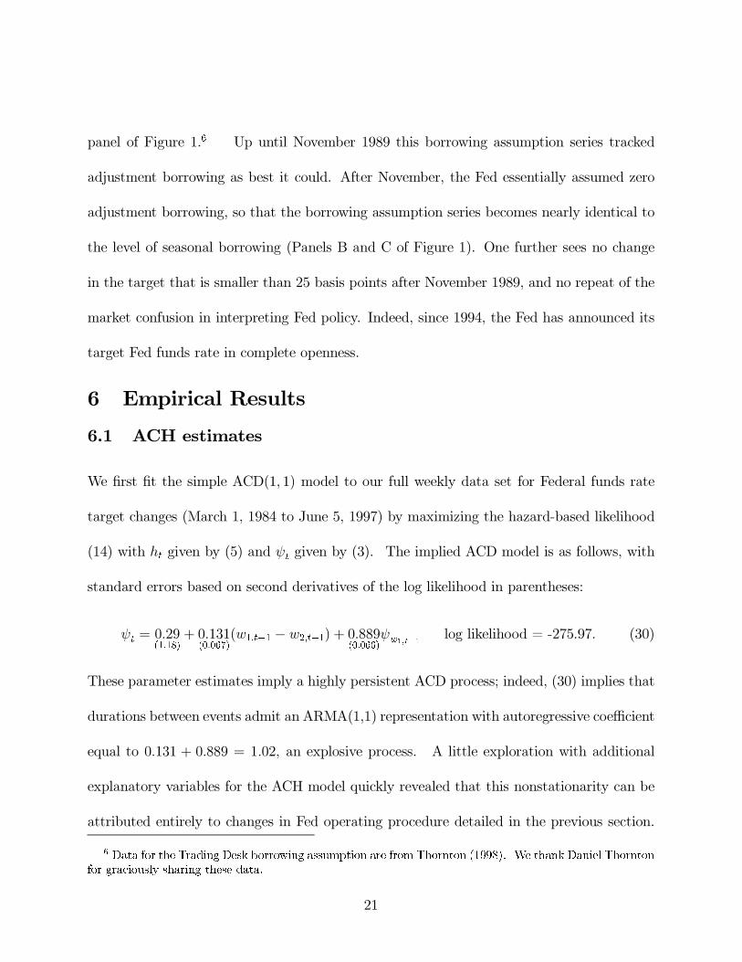
We first fit the simple ACD(1, 1) model to our full weekly data set for Federal funds rate

target changes (March 1, 1984 to June 5, 1997) by maximizing the hazard-based likelihood

(14) with ht given by (5) and ψt given by (3). The implied ACD model is as follows, with

standard errors based on second derivatives of the log likelihood in parentheses:

ψt = 0.29(1.18)

+ 0.131(0.067)

(w1,t−1 − w2,t−1) + 0.889(0.066)

ψw1,t−1log likelihood = -275.97. (30)

These parameter estimates imply a highly persistent ACD process; indeed, (30) implies that

durations between events admit an ARMA(1,1) representation with autoregressive coefficient

equal to 0.131 + 0.889 = 1.02, an explosive process. A little exploration with additional

explanatory variables for the ACH model quickly revealed that this nonstationarity can be

attributed entirely to changes in Fed operating procedure detailed in the previous section.

6 Data for the Trading Desk borrowing assumption are from Thornton (1998). We thank Daniel Thorntonfor graciously sharing these data.

21

We concluded that it is necessary to model the data as having been generated from two dif-

ferent regimes, the first corresponding to the borrowed-reserves target regime (March 1,1984

to November 23, 1989) and the second to the explicit funds-rate target regime (November

30, 1989 to June 5, 1997).

For each subsample we considered a number of variables to include in the vector zt−1

in equation (13) to try to predict the timing of changes in the target. The variables we

considered fall in three general categories: (1) variables reflecting the overall state of the

macroeconomy that may influence interest rates and the Fed’s broad policy objectives; (2)

monetary and financial aggregates; and (3) variables specific to the Trading Desk operating

procedures. For macroeconomic variables, we used the most recent figures available as of

week t. For example, the January CPI is not released until the second week of February.

Thus, for t the second through last week of January or first week of February, the component

of zt−1 corresponding to inflation would be that based on the December CPI. For the second

week of February, zt−1 would use the January CPI.

Another issue is whether to use the final revised figures or those initially released. Initial

release data are difficult to obtain for most of the series we investigated, and raise a host of

other modeling issues that seemed better to avoid in this application.7 Our final models

keep only those parameters that are statistically significant. A detailed list of all the variables

we tried is provided in Table 4.

Many of the variables that fall into the first category are motivated by papers that

7 For further discussion, see Amato and Swanson (2001), Diebold and Rudebusch (1991) Koenig, Dolams,and Piger (2000), and Runkle (1998).

22

investigate the properties of Taylor rules (such as Clarida, Gali and Gertler (2000), McCallum

and Nelson (1999), Rudebusch and Svensson (1999), and Dueker (1999b)). It is common

in this literature to model the Fed’s reaction as a function of an inflation measure (we

tried a four-quarter average of the log-change in the GDP deflator, the 12-month average

of the log-change in the personal consumption expenditures deflator, the 12-month average

of the log-change in the consumer price index less food and energy); and an output gap

measure (such as the percentage distance of actual GDP from potential GDP as measured

by the Congressional Budget Office). In addition, to allow for forward looking behavior,

we investigated the 12-month inflation forecasts from the Consumer Survey collected by

the University of Michigan along with consumer expectations on the unemployment rate

and on business conditions. To complement these data, we also experimented with the

National Association of Purchasing Manager’s composite index, and the composite indices

of coincident and leading indicators published by the Conference Board. To allow for the

possibility that the Fed reacts to deviations above or below some norm, we tried using the

absolute value of deviations from a norm (e.g., capacity utilization from 85%, GDP growth

from 2.5%, inflation from 2%, and so on).

In category (2), monetary and financial aggregates, we considered lagged values of the

Federal funds rate, M2, and the spread between 6-month Treasury Bill and the Federal

funds rate. Finally, the data contained in category (3) consisted of the dates of FOMC

meetings, Strongin’s (1995) measure of borrowed reserve pressure, the size of the previous

target change, and the duration (t− 1)−w1,t−1 since the previous change.

23

Despite an extensive literature relating Fed policy to such macroeconomic variables, we

find that for the specific task of predicting whether the Fed is going to change the target

during any given week, institutional factors and simple time-series extrapolation appear to

be far more useful than most of the above variables. Table 5 reports maximum likelihood

estimates for our favored model for the first subsample. The estimates suggest persistent

serial correlation in the durations or hazards, with α + β = 0.97. Of the variables other

than lagged durations that we investigated, only two appear to be statistically significant.

The variable FOMCt−1 is a dummy variable that takes the value of 1 if there was an FOMC

meeting during week t− 1 and is zero otherwise, while ft−1 is simply the lagged value of the

effective Fed funds rate.

The week following an FOMC meeting was considerably more likely to see a target

change than other weeks during this period. Specifically, the average value for qt in this

subsample is 1.36 and the average value for ft−1 is 6.41. These imply a typical hazard of

1/(1 + 1.36 + 4.99 − 3.40) = 0.25, or a one in four chance that the Fed would change its

target next week. By contrast, in the week following an FOMC meeting, this probability

goes up to 1/(1 + 1.36+ 4.99− 3.40− 1.58) = 0.42. A high level of the Fed funds rate also

makes the Fed more likely to adjust its target quickly. The highest levels of the Fed funds

surpass 9% at the beginning and end of the subsample, in which case the probability of a

target change rises to 1/(1+1.36+4.99−4.77) = 0.39, even with no FOMC meeting. Both

these results are entirely consistent with the description of the way the Fed implemented

and adjusted the target during this period. What is perhaps surprising is that forecasting a

24

target change over this period appears to be entirely a matter of modeling the way the Fed

responded to immediate reserve pressures and the fact of an FOMC meeting; none of the

macroeconomic variables we investigated helped improve the forecasts of target changes.

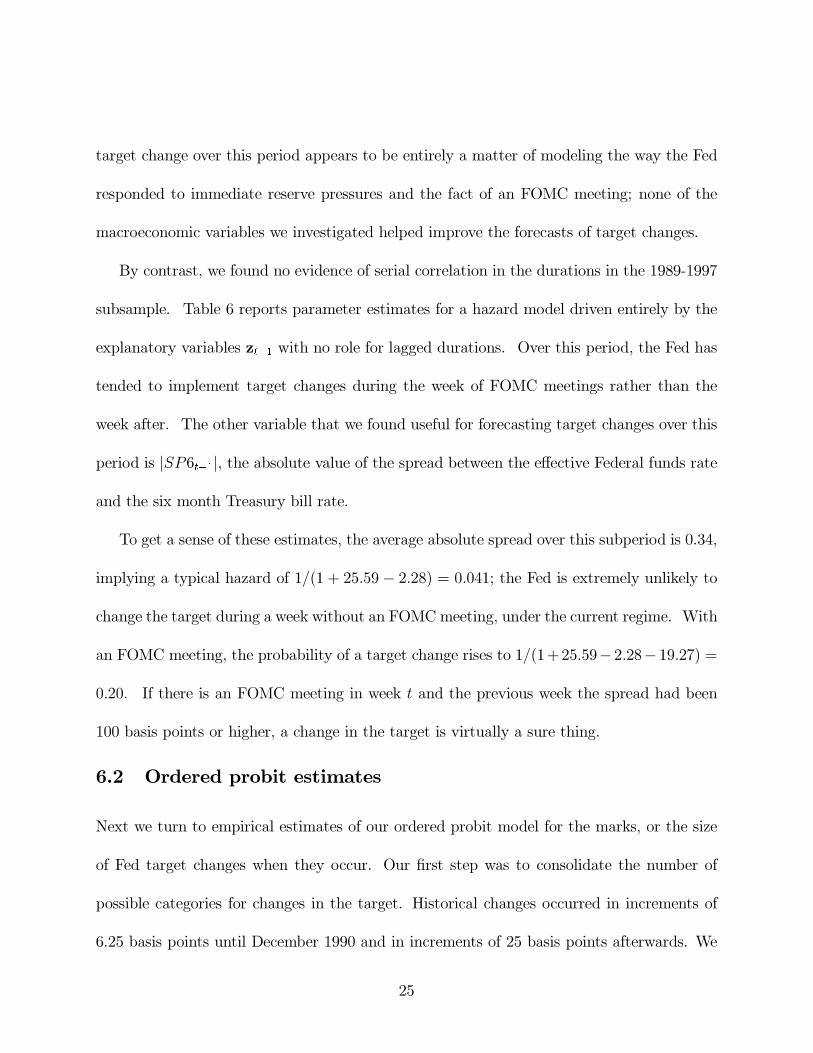
By contrast, we found no evidence of serial correlation in the durations in the 1989-1997

subsample. Table 6 reports parameter estimates for a hazard model driven entirely by the

explanatory variables zt−1 with no role for lagged durations. Over this period, the Fed has

tended to implement target changes during the week of FOMC meetings rather than the

week after. The other variable that we found useful for forecasting target changes over this

period is |SP6t−1|, the absolute value of the spread between the effective Federal funds rate

and the six month Treasury bill rate.

To get a sense of these estimates, the average absolute spread over this subperiod is 0.34,

implying a typical hazard of 1/(1 + 25.59− 2.28) = 0.041; the Fed is extremely unlikely to

change the target during a week without an FOMCmeeting, under the current regime. With

an FOMC meeting, the probability of a target change rises to 1/(1+25.59− 2.28− 19.27) =

0.20. If there is an FOMC meeting in week t and the previous week the spread had been

100 basis points or higher, a change in the target is virtually a sure thing.

6.2 Ordered probit estimates

Next we turn to empirical estimates of our ordered probit model for the marks, or the size

of Fed target changes when they occur. Our first step was to consolidate the number of

possible categories for changes in the target. Historical changes occurred in increments of

6.25 basis points until December 1990 and in increments of 25 basis points afterwards. We

25

consolidated these earlier data (along with the one change of 75 basis points on November

15, 1994) as follows. If y#i denotes the actual value for the ith target change in Table 1, then

our analyzed data yi were defined as

yi =

−0.50 if −∞ < y#i ≤ −0.5

−0.25 if −0.4375 ≤ y#i < −0.125

0.00 if −0.125 ≤ y#i < 0.0625

0.25 if 0.0625 ≤ y#i < 0.375

0.50 if 0.4375 ≤ y#i < ∞

. (31)

We then maximized the likelihood function L2(θ2) in expression (29) with respect to π,

the coefficients on the explanatory variables in (26), and the threshold parameters cj in

(28). The explanatory variables wi use the value of the variable for the week prior to the

target change. Results are reported in Table 7. Most of the ACH explanatory variables

proved insignificant for explaining the size of target changes and were dropped. We find an

extremely strong effect of yw1,t−1; if the previous change raised the target, then this week’s

change is much more likely to be an increase than a decrease. We find an equally dramatic

negative influence of the ft−1 − TB6t−1 spread; if the Fed funds rate is above the 6-month

Treasury bill rate, then we can expect the Fed to lower the target.

7 Forecast evaluations

One advantage of the ACH framework is that it generates a closed-form expression for the

one-period-ahead forecast of the target it+1 based on observation ofΥt = (it, z′

t, it−1, z

′

t−1, ...)′

26

where zt = (ft, SP6t)′. Specifically,

E(it+1|Υt) = (1− ht+1)it + ht+1

5∑j=1

(it + sj)[Φ(cj −Υ′

tπ)− Φ(cj−1 −Υ′

tπ)] (32)

where ht+1 is calculated from (13) and (7)-(10), sj = (0.25)(j − 3), cj are as given in Table

7 with c0 = −∞ and c5 = ∞ and Υ′

tπ = 2.60(iw1,t− iw2,t)− 0.42 SP6t.

Multiperiod-ahead forecasts are substantially less convenient. One first requires forecasts

of the explanatory variables zt+j. These can be generated with a VAR (with contempora-

neous values of it included), estimated for each of the two sub-samples we consider at the

November 23, 1989 break-point. Thus, for example, our forecasting equations for ft and

SP6t estimated by OLS over t = 3/8/84 to 11/23/89 are (standard errors in parenthesis):

ft = 0.218(0.091)

+ 0.347(0.069)

ft−1 − 0.042(0.047)

SP6t−1 + 0.415(0.124)

it − 0.219(0.130)

it−1, (33)

SP6t = −0.184(0.098)

− 0.492(0.073)

ft−1 + 0.886(0.050)

SP6t−1 − 0.065(0.132)

it + 0.549(0.139)

it−1. (34)

Unfortunately, the forecast E(it+j+1|Υt+j) in (32) is a nonlinear function of Υt+j, so simu-

lation methods are necessary for multiperiod-ahead forecasts. Specifically, (32) is derived

from a discrete probability distribution for it+1|Υt and one can generate a value i(1)t+1 from this

distribution. If one further assumes that the errors in (33) and (34) are bivariate Gaussian,

then, given this value i(1)t+1, can generate a value z

(1)t+1 from (33) and (34), which represents a

draw from the distribution of zt+1|Υt. Using z(1)t+1 one can again use the distribution behind

(32) to generate a value i(1)t+2, which now represents a draw from the distribution it+2|Υt.

Iterating on this sequence produces at step j a value i(1)t+j which represents a single draw

27

from the distribution f(it+j|Υt). One can then go back to the beginning to generate a

second value i(2)t+1 from f(it+1|Υt) as in (32) and iterate to obtain a second draw i

(2)t+j from

f(it+j|Υt). The average value from M simulations, M−1∑M

m=1 i(m)t+j , represents the forecast

E(it+j|Υt).

Most of the macro literature has focused on monthly values for the effective Fed funds

rate rather than the weekly Fed funds target as here. For purposes of comparison, we

estimated a monthly VAR similar to that used by Evans and Marshall (1998). The Evans-

Marshall VAR uses monthly data on the logarithm of nonagricultural employment (EM); the

logarithm of personal consumption expenditures deflator in chain-weighted 1992 dollars (P );

the change in the index of sensitive materials prices (PCOM); the effective Federal funds

rate (f); the ratio of nonborrowed reserves plus extended credit to total reserves (NBRX);

and the log growth rate of the monetary aggregate M2 (M2). The model has twelve lags and

is estimated over the sample January 1965 to September 1997. The mean squared errors

for 1- to 12-month ahead forecasts for this VAR are reported in the first column of Table 8.

We then ask, How good a job can our weekly model of the Fed funds target do at

predicting the monthly values of the effective Fed funds rate? We used our ACH and

ordered-probit model to forecast the value that the Fed funds target would assume the last

week of month τ + j based on information available as of the last week of month τ . We then

calculated the squared difference between this forecast for the target and the actual value

for the effective Fed funds rate for month τ + j and report the MSE’s in the second column

of Table 8.

28

This would seem to be a tough test for our model, given that (a) the estimation criteria for

the VAR is minimizing the MSE whereas the estimation criteria for our model is maximizing

the likelihood function; and (b) the VAR is specifically optimized for forecasting monthly

values of f whereas ours is designed to describe weekly changes in the target. Even so,

attention to the short-run institutional details of Fed policy seems to yield substantially

superior forecasts of the monthly f at horizons up to 6 months. Beyond 6 months, the

monthly VAR begins to do a significantly better job than our weekly model.8

We conclude that the ACH specification is worth considering as a realistic description

of the dynamics of the Fed funds target. It thus seems of interest to revisit some of the

policy questions that have been addressed using linear VAR’s, to which we turn in the next

section.

8 Estimating the effects of monetary policy shocks

A great number of papers have attempted to measure the effects of monetary policy based

on linear vector autoregressions. Let yτ denote a vector of macro variables for month τ ;

in the Evans and Marshall (1998) VAR, yτ = (EMτ , Pτ , PCOMτ , fτ , NBRXτ ,M2τ)′. Let

y1τ = (EMτ , Pτ , PCOMτ)′ denote the variables that come before the effective Fed funds

rate fτ and y2τ = (NBRXτ ,M2τ )′ the variables that come after. An estimate of the effects

of a monetary policy shock based on a Cholesky decomposition of the residual variance-

8 See Rudebusch (1995) for further discussion of the properties of forecasts of the target over intermediatehorizons.

29

covariance matrix would calculate the impulse-response function,

∂E(yτ+s|fτ ,y1τ ,yτ−1,yτ−2, ...)

∂fτ.

This is equivalent to finding the effect on yτ+s of an orthogonalized shock to fτ , where an

orthogonalized shock is defined as

ufτ = fτ −E (fτ |y1τ ,yτ−1,yτ−2, ...) .

Note that the shock can be written as

ufτ = fτ − fτ−1 − [E (fτ |y1τ ,yτ−1,yτ−2, ...)− fτ−1]. (35)

A positive value for ufτ could thus come from two sources. On the one hand, the Fed could

have changed the target (fτ−fτ−1 > 0) when no change was expected (E (fτ |y1τ ,yτ−1,yτ−2, ...)−

fτ−1 = 0). On the other hand, the Fed may not have changed the target (fτ − fτ−1 = 0)

even though the VAR had expected a drop (E (fτ |y1τ ,yτ−1,yτ−2, ...) − fτ−1 < 0). Either

event would produce a positive ufτ . The two events are predicted to have the same effect if

the data were generated from a linear VAR.

In a nonlinear model such as our ACH specification, however, the two events are not

forced to have the same effects, and it is an interesting exercise to see what the model says

about their respective consequences. To do so, we start with the linear VAR,

yτ = c+Φ1yτ−1 +Φ2yτ−2 + ...+Φ12yτ−12 + ετ .

We estimate the parameters (c,Φ1,Φ2, ...,Φ12) by OLS equation by equation. We also

need the forecast of y2τ given y1τ and iτ . This can be obtained by estimating the following

30

system by OLS, one equation at a time,

y2τ = d+ d1iτ +D0y1τ +B1yτ−1 +B2yτ−2 + ... +B12yτ−12 + u2τ , (36)

where d1 in the Evans-Marshall example is a (2 × 1) vector, D0 is a (2 × 3) matrix, and

Bj are (2 × 6) matrices. Given any hypothesized value for iτ and the historical values for

y1τ ,yτ−1,yτ−2, ..., one can then calculate the forecast y2τ |τ(iτ) from (36). Collect these

forecasts along with the historical y1τ and the hypothesized iτ in a vector

yτ |τ(iτ) = (y′

1τ , iτ , y′

2τ |τ(iτ))′. (37)

The one-step-ahead VAR forecast conditional on the hypothetical iτ is:

E(yτ+1|iτ ,y1τ ,yτ−1,yτ−2, ...) = c+Φ1yτ |τ(iτ) +Φ2yτ−1 + ...+Φ12yτ−11. (38)

We then replace the fourth element of the vector of conditional forecasts in (38), correspond-

ing to the forecast of the effective Fed funds rate fτ+1, with the forecast target rate for the

last week of month τ + 1. This forecast is calculated as in the previous section based on

historical values of variables available at date τ , with the historical value for the target at

date τ replaced by the hypothesized value of iτ . Call the resulting vector yτ+1|τ(iτ ). Next,

we use the VAR coefficients to generate two-step-ahead forecasts conditional on iτ :

E(yτ+2|iτ ,y1τ ,yτ−1,yτ−2, ...) = c+Φ1yτ+1|τ(iτ) +Φ2yτ |τ(iτ) + ... +Φ12yτ−10. (39)

We again replace the fourth element of (39) with the forecast of iτ+2 implied by the ACH

model and call the result yτ+2|τ(iτ). Iterating in this manner, we can calculate yτ+j|τ(iτ),

31

which summarizes the dynamic consequences of the forecast time path for iτ , iτ+1, ... implied

by the ACH model for other macroeconomic variables of interest.

To measure the consequences of the first term in (35), we ask, What difference does

it make if the Fed raises the target by 25 basis points during month τ (iτ = iτ−1 + 0.25)

compared to if it had kept the target constant (iτ = iτ−1)? We then normalize the answer

in units of a derivative, as

(0.25)−1[yτ+j|τ(iτ)

∣∣iτ=iτ−1+0.25 − yτ+j|τ(iτ)

∣∣iτ=iτ−1

]. (40)

If we had not replaced the fourth element of (38) and (39) at each iteration with the ACH

forecast, the resulting value in (40) would not depend on τ or iτ−1 and would be numerically

identical to the standard VAR impulse-response function based on the Cholesky decomposi-

tion. As is, the value of (40) does depend on τ and iτ−1, and to report results we therefore

average (40) over the historical values τ = 1, ..., T and y1, ...,yT in our sample.

The second term in (35) asks, What would happen if we predicted a change in the target

but none occurred? Letting ıτ |τ−1 denote the forecast for the target in month τ based on

historical information available at date τ − 1, we thus calculate

ωτ

[yτ+j|τ(iτ )

∣∣iτ=iτ−1 − yτ+j|τ(iτ)

∣∣∣iτ=ıτ|τ−1

](41)

where

ωτ =

(iτ−1 − ıτ |τ−1)−1 if |iτ−1 − ıτ |τ−1| > 0.02

0 otherwise

.

The effect of the weight ωτ in (41) is to ignore observations for which no change was expected

and to rescale positive or negative forecast errors into units comparable to (40). Again if we

32

had not replaced the VAR forecasts of fτ+j with the ACH forecasts of iτ+j, the magnitude

in (41) would be not depend on τ and would be numerically identical to the VAR impulse-

response function.

Figure 2 calculates the effects of three different kinds of monetary policy shocks. The

solid line is the linear VAR impulse-response function, describing the effects of a 100-basis-

point increase in fτ on each of the five other variables in yτ+j for j = 0 to 11 months. This

replicates the conventional results — an increase in the Federal funds rate is associated with

an initial decrease in nonborrowed reserves and in M2, and is followed within 6 months by a

decline in employment and prices. The short-dashed line records the average values of (40)

over all the dates τ in our sample, which we interpret as the answer to the question, What

happens when the Federal Reserve deliberately raises its target for the Federal funds rate?

The effects are qualitatively similar to the VAR impulse-response function, but quantitatively

are much bigger — a policy change implies a bigger contraction in NBRX or M2 than the

orthogonalized VAR innovations ufτ , and the negative consequences for employment and

prices are much bigger as well. The long-dashed line records the average values of (41), which

answers the question, What happens if one would have predicted that the Fed was going to

lower the target, but in fact it did not? The results are completely different, and suggest that

the Fed’s decision not to lower the target is typically an endogenous response to the Fed’s

accurate predictions of a strong economy and surging prices andmoney demand. Specifically,

if the Fed bases its decision not to lower the target on information it has about the economy

that is omitted from the VAR, it may be optimal to revise one’s forecast of GDP upward

33

on receiving the news that the Fed has not lowered the target, if the information about

the strong economy is more important than the dampening effect on growth of maintaining

high interest rates. This effect would be similar to the widely discussed price puzzle (see,

for example, Sims, 1992 and Christiano, Eichenbaum, and Evans, 1996). The linear VAR,

which essentially is an average of these two scenarios, thus appears to be mixing together

the answers to two very different experiments.

9 Conclusions

This paper introduced the autoregressive conditional hazard model for generating a time-

varying serially dependent probability forecast for a discrete event such as a change in the

Federal funds rate targeted by the Federal Reserve. The advantage over the closely related

autoregressive conditional duration specification is the ability to incorporate new information

on other variables into the forecast.

We find that the change in Federal Reserve operating procedures from borrowed re-

serves targeting over 1984-1989 to an explicit Fed funds rate target since 1989 show up quite

dramatically through this investigation. We also find that, in our nonlinear model, “inno-

vations” in monetary policy are not all the same. Specifically, an increase in the target

results in a much more dramatic effect on employment and prices than does the prediction

of a target decrease that fails to materialize.

34

References

Amato, Jefferey D. and Norman R. Swanson, (2001), “The Real-Time Predictive Con-tent of Money for Output,” Jounral of Monetary Economics, forthcoming.

Cargnoni, Claudia, Peter Müller, and Mike West, (1997), “Bayesian Forecasting ofMultinomial Time Series Through Conditionally Gaussian Dynamic Models,” Journalof the American Statistical Association 92, 640-647.

Chiang, Chin Long, (1980). An Introduction to Stochastic Processes and Their Appli-cations. New York: Krieger Publishing Co.

Christiano, Lawrence J., Martin Eichenbaum, and Charles Evans, (1996), “The Effectsof Monetary Policy Shocks: Evidence from the Flow of Funds,” Review of Economicsand Statistics, 78, 16-43.

Clarida, Richard, Jordi Gali and Mark Gertler, (2000), “Monetary Policy Rules andMacroeconomic Stability: Evidence and Some Theory,” Quarterly Journal of Eco-nomics, 115, 147-180.

Cook, Timothy and Thomas Hahn, (1989), “The Effect of Changes in the Federal FundsRate Target on Market Interest Rates in the 1970’s,” Journal of Monetary Economics24, 331-51.

Davutyan, Nurhan, and William R. Parke (1995), “The Operations of the Bank ofEngland, 1890-1908: A Dynamic Probit Approach,” Journal of Money, Credit, andBanking 27, 1099-1112.

Diebold, Francis X., and Glenn Rudebusch, (1991), “Forecasting Output with theComposite Leading Index: A Real-Time Analysis,” Journal of the American StatisticalAssociation, 86, 603-610.

Dueker, Michael, (1999a), “Conditional Heteroscedasticity in Qualitative ResponseModels of Time Series: A Gibbs-Sampling Approach to the Bank Prime Rate,” Journalof Business and Economic Statistics, 17, 466-472.

_____, (1999b), “Measuring Monetary Policy Inertia in Target Fed Funds RateChanges,” Federal Reserve Bank of St. Louis Review, 81(5), 3-9.

Dufour, Alfonso, and Robert F. Engle, (1999), “The ACD Model: Predictability of theTime between Consecutive Trades,” working paper, UCSD.

Eichengreen, Barry, Mark W. Watson, and Richard S. Grossman, (1985), “Bank RatePolicy under the Interwar Gold Standard: A Dynamic Probit Model,” Economic Jour-nal 95, 725-745.

35

Engle, Robert F., (2000), “The Econometrics of Ultra-High-Frequency Data,” Econo-metrica, 68, 1-22.

_____, and Jeffrey R. Russell, (1997), “Forecasting the Frequency of Changes inQuoted Foreign Exchange Prices with the ACD Model,” Journal of Empirical Finance,12, 187-212.

_____, and _____ (1998), “Autoregressive Conditional Duration: A New Modelfor Irregularly Spaced Transaction Data,” Econometrica 66, 1127-1162.

_____, and _____ (1999), “The Econometric Analysis of Discrete-ValuedIrregularly-Spaced Financial Transactions Data Using a New Autoregressive Condi-tional Multinomial Model,” working paper, UCSD.

Evans, Charles L., and David A. Marshall (1998), “Monetary Policy and the TermStructure of Nominal Interest Rates: Evidence and Theory,” Carnegie-Rochester Con-ference Series on Public Policy, 49, 53-111.

Fahrmeir, Ludwig, (1992), “Posterior Mode Estimation by Extended Kalman Filter-ing for Multivariate Dynamic Generalized linear Models,” Journal of the AmericanStatistical Association, 87, 501-509.

_____, (1994), “Dynamic Modelling and Penalized Likelihood Estimation for Dis-crete Time Survival Data,” Biometrica, 81, 317-330.

Federal Reserve Bank of New York, (1990), “Monetary Policy and Open Market Op-erations During 1989,” A Report prepared for the Federal Open Market Committeeby the Open Market Group of the Federal Reserve Bank of New York, March 1990,confidential.

Feinman, Joshua, (1993), “Estimating the Open Market Desk’s Daily Reaction Func-tion,” Journal of Money, Credit, and Banking, 25, 231-47.

Hausman, Jerry A., Andrew W. Lo and A. Craig Mackinlay, (1992), “An OrderedProbit Analysis of Transaction Stock Prices,” Journal of Financial Economics 31,319-379.

Heller, H. Robert, (1988), “Implementing Monetary Policy,” Federal Reserve BulletinJuly, 419-429.

Koenig, Evan F., Sheila Dolmas, and Jeremy Piger, (2000), “The Use and Abuse of‘Real-Time’ Data in Economic Forecasting,” International Finance Discussion Paper2000-684, Board of Governors of the Federal Reserve.

Lee, Lung-fie, (1999), “Estimation of Dynamic and ARCH Tobit Models,” Journal ofEconometrics, 92, 355-390.

36

Lunde, Asger, and Allan Timmermann, (2000), “Duration Dependence in Stock Prices:An Analysis of Bull and Bear Markets,” working paper, University of California, SanDiego.

McCallum, Bennett T. and Edward Nelson, (1999), “Performance of Operational Pol-icy Rules in an Estimated Semiclassical Structural Model,” in Monetary Policy Rules,John B. Taylor (ed.), Chicago: The University of Chicago Press.

McCulloch, Robert, and Peter E. Rossi, (1994), “An Exact Likelihood Analysis of theMultinomial Probit Model,” Journal of Econometrics, 64, pp. 207-240.

Meulendyke, AnnMarie, (1998), U. S. Monetary Policy and Financial Markets, FederalReserve Bank of New York.

Piazzesi, Monika, (2000), “An Econometric Model of the Yield Curve with Macroeco-nomic Jump Effects,” working paper, Stanford University.

Rudebusch, Glenn D., (1995), “Federal Reserve Interest Rate Targeting, Rational Ex-pectations and the Term structure,” Journal of Monetary Economics 35, 245-74. Er-ratum: (December 1995) 36:679.

_____, and Lars E. O. Svensson, (1999), “Policy Rules for Inflation Targeting,”in Monetary Policy Rules, John B. Taylor (ed.), Chicago: The University of ChicagoPress.

Runkle, David E. (1998), “Revisionist History: How Data Revisions Distort EconomicPolicy Research,” Federal Reserve Bank of Minneapolis Economic Review, Fall, 3-12.

Sims, Christopher A., (1992), “Interpreting the Macroeconomic Time Series Facts:The Effects of Monetary Policy,” European Economic Review 36, 975-1000.

Strongin, Steven, (1995), “The Identification of Monetary Policy Disturbances. Ex-plaining the Liquidity Puzzle,” Journal of Monetary Economics 35, 463-497.

Thornton, Daniel L., (1998), “The Federal Reserve’s Operating Procedure, Nonbor-rowed Reserves, Borrowed Reserves, and the Liquidity Effect,” working paper, FederalReserve Bank of St. Louis.

37

Table 1 - Calendar of Changes in the Federal Funds Rate Target Date of Target Target Duration Day of Date of Target Target Duration Day of Change Value Change in days the Week Change Value Change in days the Week 1-Mar-84 9.5 na Thursday 28-Jan-88 6.625 -0.1875 85 Thursday

15-Mar-84 9.875 0.375 14 Thursday 11-Feb-88 6.5 -0.125 14 Thursday 22-Mar-84 10 0.125 7 Thursday 30-Mar-88 6.75 0.25 48 Wednesday 29-Mar-84 10.25 0.25 7 Thursday 9-May-88 7 0.25 40 Monday

5-Apr-84 10.5 0.25 7 Thursday 25-May-88 7.25 0.25 16 Wednesday 14-Jun-84 10.625 0.125 70 Thursday 22-Jun-88 7.5 0.25 28 Wednesday 21-Jun-84 11 0.375 7 Thursday 19-Jul-88 7.6875 0.1875 27 Tuesday 19-Jul-84 11.25 0.25 28 Thursday 8-Aug-88 7.75 0.0625 20 Monday 9-Aug-84 11.5625 0.3125 21 Thursday 9-Aug-88 8.125 0.375 1 Tuesday

30-Aug-84 11.4375 -0.125 21 Thursday 20-Oct-88 8.25 0.125 72 Thursday 20-Sep-84 11.25 -0.1875 21 Thursday 17-Nov-88 8.3125 0.0625 28 Thursday 27-Sep-84 11 -0.25 7 Thursday 22-Nov-88 8.375 0.0625 5 Tuesday

4-Oct-84 10.5625 -0.4375 7 Thursday 15-Dec-88 8.6875 0.3125 23 Thursday 11-Oct-84 10.5 -0.0625 7 Thursday 29-Dec-88 8.75 0.0625 14 Thursday 18-Oct-84 10 -0.5 7 Thursday 5-Jan-89 9 0.25 7 Thursday 8-Nov-84 9.5 -0.5 21 Thursday 9-Feb-89 9.0625 0.0625 35 Thursday

23-Nov-84 9 -0.5 15 Friday 14-Feb-89 9.3125 0.25 5 Tuesday 6-Dec-84 8.75 -0.25 13 Thursday 23-Feb-89 9.5625 0.25 9 Thursday

20-Dec-84 8.5 -0.25 14 Thursday 24-Feb-89 9.75 0.1875 1 Friday 27-Dec-84 8.125 -0.375 7 Thursday 4-May-89 9.8125 0.0625 69 Thursday 24-Jan-85 8.25 0.125 28 Thursday 6-Jun-89 9.5625 -0.25 33 Tuesday 14-Feb-85 8.375 0.125 21 Thursday 7-Jul-89 9.3125 -0.25 31 Friday 21-Feb-85 8.5 0.125 7 Thursday 27-Jul-89 9.0625 -0.25 20 Thursday 21-Mar-85 8.625 0.125 28 Thursday 10-Aug-89 9 -0.0625 14 Thursday 28-Mar-85 8.5 -0.125 7 Thursday 18-Oct-89 8.75 -0.25 69 Wednesday 18-Apr-85 8.375 -0.125 21 Thursday 6-Nov-89 8.5 -0.25 19 Monday 25-Apr-85 8.25 -0.125 7 Thursday 20-Dec-89 8.25 -0.25 44 Wednesday

16-May-85 8.125 -0.125 21 Thursday 13-Jul-90 8 -0.25 205 Friday 20-May-85 7.75 -0.375 4 Monday 29-Oct-90 7.75 -0.25 108 Monday

11-Jul-85 7.6875 -0.0625 52 Thursday 14-Nov-90 7.5 -0.25 16 Wednesday 25-Jul-85 7.75 0.0625 14 Thursday 7-Dec-90 7.25 -0.25 23 Friday

22-Aug-85 7.8125 0.0625 28 Thursday 19-Dec-90 7 -0.25 12 Wednesday 29-Aug-85 7.875 0.0625 7 Thursday 9-Jan-91 6.75 -0.25 21 Wednesday

6-Sep-85 8 0.125 8 Friday 1-Feb-91 6.25 -0.5 23 Friday 18-Dec-85 7.75 -0.25 103 Wednesday 8-Mar-91 6 -0.25 35 Friday 7-Mar-86 7.25 -0.5 79 Friday 30-Apr-91 5.75 -0.25 53 Tuesday

10-Apr-86 7.125 -0.125 34 Thursday 6-Aug-91 5.5 -0.25 98 Tuesday 17-Apr-86 7 -0.125 7 Thursday 13-Sep-91 5.25 -0.25 38 Friday 24-Apr-86 6.75 -0.25 7 Thursday 31-Oct-91 5 -0.25 48 Thursday

22-May-86 6.8125 0.0625 28 Thursday 6-Nov-91 4.75 -0.25 6 Wednesday 5-Jun-86 6.875 0.0625 14 Thursday 6-Dec-91 4.5 -0.25 30 Friday

11-Jul-86 6.375 -0.5 36 Friday 20-Dec-91 4 -0.5 14 Friday 14-Aug-86 6.3125 -0.0625 34 Thursday 9-Apr-92 3.75 -0.25 111 Thursday 21-Aug-86 5.875 -0.4375 7 Thursday 2-Jul-92 3.25 -0.5 84 Thursday

4-Dec-86 6 0.125 105 Thursday 4-Sep-92 3 -0.25 64 Friday 30-Apr-87 6.5 0.5 147 Thursday 4-Feb-94 3.25 0.25 518 Friday

21-May-87 6.75 0.25 21 Thursday 22-Mar-94 3.5 0.25 46 Tuesday 2-Jul-87 6.625 -0.125 42 Thursday 18-Apr-94 3.75 0.25 27 Monday

27-Aug-87 6.75 0.125 56 Thursday 17-May-94 4.25 0.5 29 Tuesday 3-Sep-87 6.875 0.125 7 Thursday 16-Aug-94 4.75 0.5 91 Tuesday 4-Sep-87 7.25 0.375 1 Friday 15-Nov-94 5.5 0.75 91 Tuesday

24-Sep-87 7.3125 0.0625 20 Thursday 1-Feb-95 6 0.5 78 Wednesday 22-Oct-87 7.125 -0.1875 28 Thursday 6-Jul-95 5.75 -0.25 155 Thursday 28-Oct-87 7 -0.125 6 Wednesday 19-Dec-95 5.5 -0.25 166 Tuesday 4-Nov-87 6.8125 -0.1875 7 Wednesday 31-Jan-96 5.25 -0.25 43 Wednesday

25-Mar-97 5.50 0.25 419 Tuesday

Table 2: Dates of Federal Open Markets Committee Meetings Year FOMC Dates Year FOMC Dates 1984 January 30-31 1991 February 5-6

March 26-27 March 26 May 21-22 May 14 July 16-17 July 2-3 August 21 August 20 October 2 October 1 November 7 November 5 December 17-18 December 17-18

1985 February 12-13 1992 February 4-5 March 26 March 31 May 21 May 19 July 9-10 June 30-31 August 20 August 18 October 1 October 16 November 4-5 November 17 December 16-17 December 22

1986 February 11-12 1993 February 2-3 April 1 March 23 May 20 May18 July 8-9 July 6-7 August 19 August 17 September 23 September 21 November 5 November 16 December 15-16 December 21

1987 February 10-11 1994 February 3-4 March 31 March 22 May 19 May 17 July 7 July 5-6 August 18 August 16 September 22 September 27 November 3 November 15 December 15-16 December 20

1988 February 9-10 1995 January 31-1 March 29 March 28 May 17 May 23 June 29-30 July 5-6 August 16 August 22 September 30 September 26 November 1 November 15 December 13-14 December 19

1989 February 6-7 1996 January 30-31 March 28 March 26 May 16 May 21 July 5-6 July 2-3 August 22 August 20 October 3 September 24 November 14 November 13 December 18-19 December 17

1990 February 6-7 1997 February 4-5 March 27 March 25 May 15 May 20 July 2-3 July 1-2 August 21 August 19 October 2 September 30 November 13 November 12 December 17-18 December 16

Table 3: Dates of FOMC Telephone Conference Calls

Year Date of Call Year Date of Call 1984 January 11 1989 February 23

March 20 May 31 October 18 June 5 December 7 July 26

1985 January 18 October 16 September 10 October 17 September 23 October 18

1986 January 17 November 6 April 21 November 27

1987 February 23 1990 January 16 April 29 April 11 October 20 August 6 October 21 September 7 October 22 September 17 October 23 December 7 October 26 1991 January 9 October 27 February 1 October 28 March 26 October 29 April 12 October 30 April 30

1988 January 5 May 1 May 6 June 10 May 24 June 24 June 22 August 5 July 19 September 13 August 5 October 30 August 9 December 2 October 17 December 20 November 22 1992 January 9 March 11 July 2 December 14 1993 January 6 February 18 March 1 October 5 October 15 October 22

Table 4

List of candidate explanatory variables in the specification of the ACH model

Inflation Measures:

• GDP Deflator (yearly average of the annualized log-change, in percent)

• CPI Index, less food and energy (yearly average of the annualized log-change, in per-

cent)

• Personal Consumption Expenditures Deflator (yearly average of the annualized log-

change, in percent)

• Employment Cost Index (annualized, quarterly log-change, in percent)

• 12-month ahead inflation forecasts (Consumer Survey, University of Michigan)

Output Measures:

• Output Gap (log difference between actual and potential GDP, Congressional Budget

Office estimates, in percent)

• GDP growth (annualized quarterly growth rate, in percent)

• Total Capacity Utilization (in deviations from an 80% norm)

• 12-month ahead consumer expectations on business conditions (Consumer Survey, Uni-

versity of Michigan)

40

• National Association of Purchasing Manager’s composite index

Employment Measures:

• Unemployment Rate

• 12-month ahead consumer expectations on unemployment (Consumer Survey, Univer-

sity of Michigan)

Other Activity Measures:

• Budget Deficit/Surplus

• Composite Index of coincident and leading indicators (The Conference Board)

Monetary Variables:

• M2 (log change in percent)

• Federal funds rate

• 6-month Treasury Bill Spread (relative to the Federal funds rate)

Trading Desk Variables:

• Discount Window borrowing (normalized by lagged total reserves)

• FOMC meeting dates

41

Table 5

Parameter Estimates for ACH(1,1) Model for 1984-1989

parameter variable estimate (standard error)

α w1,t−1 − w2,t−1 0.085 (0.058)

β qw1,t−10.886 (0.109)

δ1 constant 4.991 (2.305)

δ2 FOMCt−1 -1.579 (0.691)

δ3 ft−1 -0.530 (0.212)

log likelihood: -162.27

Variable Definitions:

• w1,t−1−w2,t−1 : duration between the two most recent target changes as of week t− 1.

• qw1,t−1: lagged value of the latent index q, dated as of the time of the last target change

since date t− 1.

• FOMCt−1 : dummy variable that takes the value of 1 if in week t − 1, there was an

FOMC meeting, 0 otherwise.

• ft−1 : value of the federal funds rate target at time t− 1.

42

Table 6

Parameter Estimates for ACH(0,0) Model for 1989-1997

parameter variable estimate (standard error)

δ1 constant 25.59 (6.38)

δ2 FOMCt -19.27 (6.35)

δ3 |SP6t−1| -6.70 (2.61)

log likelihood: -85.39

Variable definitions:

• FOMCt : dummy variable that takes the value of 1 if in week t, there was an FOMC

meeting, 0 otherwise.

• |SP6t−1| : absolute value of the spread between the six month T-Bill and the federal

funds rate.

43

Table 7

Parameter Estimates for Ordered Probit Model for 1984-1997

parameter variable estimate (standard error)

π1 yw1,t−12.60 (0.41)

π2 SP6t−1 -0.42 (0.22)

c1 -1.85 (0.23)

c2 -0.38 (0.19)

c3 0.05 (0.19)

c4 1.56 (0.24)

log likelihood: -122.97

Variable Definitions:

• yw1,t−1: magnitude of the last target change as of date t− 1.

• SP6t−1 :value of the spread between the six month T-Bill and the federal funds rate.

44

Table 8

Mean Squared Errors for 1-12 Step-Ahead Forecasts Based on

the ACH model and the VAR from Evans and Marshall (1998)

Forecast horizon VAR ACH

1 Month Ahead 0.1052 0.0242

2 Months Ahead 0.2051 0.0837

3 Months Ahead 0.3201 0.1849

4 Months Ahead 0.4410 0.3222

5 Months Ahead 0.5625 0.4905

6 Months Ahead 0.6843 0.6790

7 Months Ahead 0.8000 0.8944

8 Months Ahead 0.9093 1.1556

9 Months Ahead 1.0031 1.3531

10 Months Ahead 1.1139 1.9112

11 Months Ahead 1.2435 2.3862

12 Months Ahead 1.4048 2.8686

45

Figure Captions

Figure 1. Top panel: adjustment borrowing at the Fed discount window (dashed line)

and the Fed Trading Desk’s borrowing assumption (solid line). Middle panel: seasonal

borrowing at the Fed discount window (dashed line) and the Fed Trading Desk’s borrowing

assumption (solid line). Bottom panel: the borrowing assumption minus seasonal borrowing.

Figure 2. Effect on yτ+j for j = 0, 1, ..., 11 of different definitions of an ”innovation”

in the Fed funds rate. Solid line: innovation means a forecast error in the VAR. Short-

dashed line: innovation means that the Fed raised the Fed funds target. Long-dashed

line: innovation means a forecast target change that failed to materialize. Different panels

correspond to the different elements of y.

46

Adjustment borrowing and borrowing assumption

1981 1982 1983 1984 1985 1986 1987 1988 1989 1990 1991 1992 1993 1994 1995 19960

250

500

750

1000

1250

1500

1750

2000ASSUMP

ADJBOR

Seasonal borrowing and borrowing assumption

1981 1982 1983 1984 1985 1986 1987 1988 1989 1990 1991 1992 1993 1994 1995 19960

250

500

750

1000

1250

1500

1750

2000ASSUMP

SEASBOR

Borrowing assumption minus seasonal borrowing

1981 1982 1983 1984 1985 1986 1987 1988 1989 1990 1991 1992 1993 1994 1995 19960

250

500

750

1000

1250

1500

1750

2000

-0.4

-0.3

-0.2

-0.1

0.0

0.1

EMVAR EM25 EM0

Response of EM

-0.15

-0.10

-0.05

0.00

0.05

0.10

PVAR P25 P0

Response of P

-0.6

-0.4

-0.2

0.0

0.2

0.4

PCVAR PC25 PC0

Response of PCOM

-2

0

2

4

6

8

10

12

14

NBVAR NB25 NB0

Response of NBRX

-0.2

0.0

0.2

0.4

0.6

M2VAR M225 M20

Response of M2

Figure 2 -Responses to Different Measures of Innovations in the Federal Funds Rate

Notes:- 12 Lag VAR as originally estimated in Evans and Marshall, 1998 (EV).- Suffix "VAR" refers to the actual IRF from the EV paper.- Suffix "25" refers to the IRF when the target shock is 0.25.- Suffix "0" refers to the IRF when the target shock is given by expectations.

0 1 2 3 4 5 6 7 8 9 10 11 0 1 2 3 4 5 6 7 8 9 10 11

0 1 2 3 4 5 6 7 8 9 10 11 0 1 2 3 4 5 6 7 8 9 10 11

0 1 2 3 4 5 6 7 8 9 10 11