NBER WORKING PAPER SERIES

A MODEL OF AGGREGATE DEMAND AND UNEMPLOYMENT

Pascal MichaillatEmmanuel Saez

Working Paper 18826http://www.nber.org/papers/w18826

NATIONAL BUREAU OF ECONOMIC RESEARCH1050 Massachusetts Avenue

Cambridge, MA 02138February 2013

This paper was previously circulated under the title "A Theory of Aggregate Supply and AggregateDemand as Functions of Market Tightness with Prices as Parameters." We are deeply indebted to GeorgeAkerlof for his comments and suggestions. We thank Wouter den Haan, Peter Diamond, EmmanuelFarhi, Roger Farmer, Yuriy Gorodnichenko, Greg Kaplan, Phillip Kircher, Camille Landais, EtienneLehmann, Kristof Madarasz, Alan Manning, Emi Nakamura, Nicolas Petrosky-Nadeau, Pontus Rendhal,Kevin Sheedy, Jon Steinsson, Etienne Wasmer, Danny Yagan, and numerous seminar and conferenceparticipants for helpful discussions and comments. Financial support from the Center for EquitableGrowth at the University of California Berkeley and from the Fondation Banque de France is gratefullyacknowledged. Michaillat is grateful to the W.E. Upjohn Institute for Employment Research for itsfinancial support through Early Career Research Grant #12-137-09. The views expressed herein arethose of the authors and do not necessarily reflect the views of the National Bureau of Economic Research.

NBER working papers are circulated for discussion and comment purposes. They have not been peer-reviewed or been subject to the review by the NBER Board of Directors that accompanies officialNBER publications.

© 2013 by Pascal Michaillat and Emmanuel Saez. All rights reserved. Short sections of text, not toexceed two paragraphs, may be quoted without explicit permission provided that full credit, including© notice, is given to the source.

A Model of Aggregate Demand and UnemploymentPascal Michaillat and Emmanuel SaezNBER Working Paper No. 18826February 2013, Revised July 2013JEL No. E12,E24,E32,E63

ABSTRACT

We present a static model of aggregate demand and unemployment. The economy has a nonproducedgood, a produced good, and labor. Product and labor markets have matching frictions. A general equilibriumis a set of prices, market tightnesses, and quantities such that buyers and sellers optimize given pricesand tightnesses, and actual tightnesses equal posted tightnesses. In each frictional market, there is onemore variable than equilibrium condition. To close the model, we take all prices as parameters. Weobtain the following results: (1) unemployment and unsold production prevail in equilibrium; (2) eachmarket can be slack, efficient, or tight if the price is too high, efficient, or too low; (3) product markettightness and sales are positively correlated under aggregate demand shocks but negatively correlatedunder aggregate supply shocks; (4) transfers from savers to spenders stimulate aggregate demand,product market tightness, and employment; (5) the government-purchase multiplier is positive whenthe economy is slack, zero when the economy is efficient, and negative when the economy is tight;(6) with unequal distribution of profits and labor income, a wage increase may stimulate aggregatedemand and reduce unemployment.

Pascal MichaillatDepartment of EconomicsLondon School of EconomicsHoughton StreetLondon, WC2A 2AEUnited Kingdomp.michaillat@lse.ac.uk

Emmanuel SaezDepartment of EconomicsUniversity of California, Berkeley530 Evans Hall #3880Berkeley, CA 94720and NBERsaez@econ.berkeley.edu

1 Introduction

There is a view that fluctuations in aggregate demand explain some of the fluctuations in unemploy-

ment observed over the business cycle. However, the standard theory of unemployment—the match-

ing theory developed by Diamond [1982], Mortensen [1982], and Pissarides [1985]—only accounts

for fluctuations caused by changes in wages, matching process, production technology, or policy. In

this paper we propose a model that builds on matching theory and that accounts for the influence of

aggregate demand on unemployment.

The model is static. There are three goods in the economy: a nonproduced good, a produced

good, and labor. The market for nonproduced good is perfectly competitive but the product and labor

markets have matching frictions. Matching frictions have two components: a matching function,

which governs the number of trades on the market, and a matching cost, incurred by each buyer and

measured in terms of the traded good.1 From a seller’s perspective, a frictional market looks like

a competitive market except that she must take into account not only the market price but also the

probability to sell, which is less than one. From a buyer’s perspective, a frictional market looks like a

competitive market except that she must take into account the effective price of consumption, which

is the market price times a wedge that captures the cost of matching. We define a market tightness

for each frictional market. The market tightness determines the selling probability and the matching

wedge. A general equilibrium is a set of prices, market tightnesses, and quantities such that buyers

and sellers optimize given prices and tightnesses, and actual tightnesses equal posted tightnesses. In

each frictional market, there is one more variable than equilibrium condition. This property implies

that many combinations of prices and tightnesses are consistent with general equilibrium. To close

the model, we take all prices as parameters. Nonetheless, the equilibrium is pairwise Pareto efficient

in the sense that once a match is realized, there is no price change that could benefit both seller and

buyer. Since prices are parameters, only tightnesses equilibrate the markets with matching frictions.

The model has three critical elements: nonproduced good, matching frictions, and parametric

prices. The nonproduced good is necessary to obtain an interesting concept of aggregate because

without it, consumers would mechanically spend all their income on produced good. In our model

consumers allocate their income between consumptions of produced and nonproduced good, and

1By introducing these two components, we follow the common approach to modeling matching frictions. The match-ing function is a well-behaved function that summarizes the complicated exchange process between buyers an sellers. SeePetrongolo and Pissarides [2001] and Rogerson, Shimer and Wright [2005] for discussions of the theoretical foundationsand empirical characterization of the matching function. The matching cost is usually measured in terms of numeraire,but measuring it in terms of traded goods simplifies the exposition and welfare analysis. Farmer [2008, 2009] and Shimer[2010] make the same modeling choice.

1

aggregate demand is the desired consumption of produced good. Matching frictions generate un-

sold production in equilibrium to propagate aggregate demand shocks to the labor market, generate

unemployment in equilibrium, and provide a theoretical justification for price and wage rigidity in

equilibrium. Last, the parametric prices allow aggregate demand and other shocks to affect aggre-

gate demand and labor demand and to have macroeconomic effects. The reason is that the prices

do not respond to shocks, as in the Keynesian tradition. Modeling prices as parameters simplifies the

mechanics of the model while describing the short-run reasonably well as long as prices adjust slowly.

Our model is parsimonious, even when we introduce heterogeneity in preferences, wealth, labor

income, or profit income. The partial equilibrium on each market is represented by the intersection

of a demand curve and supply curve in a (quantity, tightness) plane. It is easy to solve for the general

equilibrium and obtain comparative statics since product market tightness and labor market tightness

solve a simple system of two equations. It is also easy to analyse and represent welfare. We define a

market as slack, efficient, or tight when market tightness is below, at, or above the efficient level of

tightness. In a slack market, consumption and sales—the sum of consumption and aggregate matching

costs—are too low. In a tight market, consumption is too low but sales are too high. When the market

is tight, too much of the traded good is dissipated as matching cost. Each market is slack, efficient, or

tight when the exogenous price is too high, efficient, or too low.

In Section 2, we present the simplest model connecting aggregate demand to unemployment. This

model represents an economy of self-employed workers who sell and purchase services on a market

with matching frictions. Labor and the produced good are a single good so that labor and product mar-

kets are a single market. Because of the matching frictions, workers cannot sell all their services and

are idle part of the time. The rate of idleness, which we interpret as the unemployment rate, is a nega-

tive function of market tightness. We obtain a number of results. First, we show that market tightness

and sales are positively correlated under aggregate demand shocks but negatively correlated under

aggregate supply shocks. Second, when individuals differ in their marginal propensity to consume,

transfers from savers to spenders stimulate aggregate demand and market tightness. Such transfers

increase aggregate consumption when the economy is slack but reduce it when the economy is tight.

Third, the government-purchase multiplier changes sign across economic regimes: it is positive when

the economy is slack, zero when the economy is efficient, and negative when the economy is tight.

In Section 3, we introduce firms that mediate between workers and consumers by hiring workers

on a labor market with matching frictions, employing these workers to produce goods, and selling the

production on a product market with matching frictions. Following Michaillat [2012], we assume that

firms are large, face a production function with diminishing marginal returns to labor, and maximize

2

profits taking labor market tightness and real wage as given. This richer model allows us to study

how aggregate demand shocks propagate from the product market to the labor market and how they

affect unemployment, to study the effects of shocks to technology, labor force participation, and real

wage, and to examine the impact of an unequal distribution of profits and labor income. For instance,

we show that if profits are concentrated among savers while labor income is concentrated among

spenders, a wage increase may reduce unemployment. This happens when the positive effect of the

wage increase on aggregate demand dominates its negative effect on labor demand.

Section 4 argues that our matching framework is not restrictive. Using alternative assumptions

about the functional forms of the utility, production, and matching functions, the value of matching

costs, and the price and wage schedules, our model yields the same first-order conditions as a broad

range of macroeconomic models. When we make assumptions to mimic a perfect-competition model,

a matching model with Nash bargaining over price and wage, and a monopolistic-competition model,

aggregate demand shocks have no effect because the price adjusts sufficiently to absorb them com-

pletely. In contrast in our model, price and wage are rigid and aggregate demand shocks therefore

propagate to product and labor markets. When we make assumptions to mimic a matching model

with rigid price and wage and with linear utility and production functions, many issues related to ag-

gregate demand are trivial because aggregate demand and labor demand functions are perfectly elastic

in tightness. In contrast in our model, utility function and production function are concave so the de-

mand functions are decreasing in tightness. When we make assumptions to mimic a fixprice-fixwage

model, we obtain aggregate demand effects, but the theory is much less tractable because it creates

four different regimes, each with a different set of equilibrium conditions. The four regimes appear

because the matching functions are equal to the minimum of their two arguments so all supply func-

tions have kinks. In contrast in our model, the matching functions are smooth, the kinks disappear,

and the general equilibrium is described by a unique set of equilibrium conditions.

Section 5 concludes by discussing some applications of the model. First, the model could be

used to analyze the impact on unemployment of fiscal policies that affect simultaneously aggregate

demand, labor demand, and labor supply (for example, unemployment insurance, employer and em-

ployee payroll taxes, or minimum wage). Second, empirical research could exploit the theoretical

predictions of the model to identify the macroeconomic shocks driving business cycle fluctuations.

A key result of the analysis is that product market tightness and sales are positively correlated under

aggregate demand shocks but negatively correlated under other shocks. We explain how empirical

research on sales and inventories could use this result to identify macroeconomic shocks. Third, the

model could be a starting point to build a dynamic and stochastic macroeconomic model featuring

3

unsold production and unemployment. To obtain a quantitatively realistic model, however, we would

need to introduce a process for price adjustment instead of considering fixed prices only. For instance,

prices might adjust toward the efficient level in the medium run through the competitive search mech-

anism of Moen [1997].

Our model is related to several other models that explore the link between aggregate demand and

equilibrium unemployment.2 Farmer [2008, 2009] exploits the indeterminacy arising in a matching

model of the labor market to select an equilibrium using agents’ beliefs about the level of economic

activity. In Farmer’s models, the wage satisfies an additional condition imposing that agents’ beliefs

are fulfilled in equilibrium. In contrast, in our model, price and wage are parameters. Lehmann and

Van der Linden [2010] build a matching model of the product market and labor market. Money is

required for transactions, giving rise to aggregate demand. In their model, the price is determined by

competitive search and the wage by Nash bargaining so price and wage are completely flexible. In

contrast, in our model, price and wage are parameters so they are rigid in response to macroeconomic

shocks. Rendhal [2012] builds a New Keynesian model with matching frictions in the labor market,

giving rise to unemployment, and a cash-in-advance constraint in the product market, giving rise to

an aggregate demand. Kaplan and Menzio [2013] propose a model with matching frictions on the

labor market and the search frictions of Burdett and Judd [1983] on the product market. Shopping

externalities appear, generating multiple rational-expectation equilibria and self-fulfilling fluctuations

in unemployment. The product markets are represented differently in the models of Rendhal [2012]

and Kaplan and Menzio [2013] and in ours. Thus, aggregate demand shocks propagate differently in

these models: the Euler equation and the zero lower bound play a key role in the model of Rendhal

[2012]; price dispersion is critical in the model of Kaplan and Menzio [2013]; matching frictions and

unsold production are central to our model.

2 A Basic Matching Model

This section presents the simplest model in which aggregate demand influences unemployment. All

workers are self-employed and sell services on a market with matching frictions. Because of the

matching frictions, workers may not be able to sell all their services. Thus, workers may be idle part

2Macroeconomists have recently shown renewed interest for aggregate demand. For example, see Mian and Sufi [2012]for an empirical investigation of the role of aggregate demand, Lorenzoni [2009] for a model in which news shocks act asaggregate demand shocks, Eggertsson and Krugman [2012] for a model in which debt deleveraging depresses aggregatedemand, Heathcote and Perri [2012] for a model in which a housing market crash depresses aggregate demand, and Bai,Rios-Rull and Storesletten [2012] for a model of aggregate demand based on a matching model of the product market.

4

of the time in equilibrium. Idleness corresponds to unemployment in this simple model.

2.1 The Model

Market for Services. A measure 1 of identical self-employed workers sell services on a market

with matching frictions. The capacity of each worker is y; that is, a worker would like to sell y units

of services. Workers are also consumers of services, but they cannot consume their own services.

Each consumer visits v workers to purchase their services. The number of trades between consumers

and workers is given by a matching function with constant elasticity of substitution:

s =(y−η + v−η

)− 1η ,

where η determines the elasticity of substitution between inputs in the matching process.3 We impose

η > 0 such that the number of trades is less than aggregate capacity, y, and less than the total number

of visits, v. In each trade, a consumer buys one unit of service from a worker at price p > 0.

We define market tightness as the ratio of visits to capacity: x ≡ v/y. Since the matching function

displays constant returns to scale, market tightness determines the probabilities that one unit of service

is sold and that one visit leads to a purchase. Workers sell each unit of service with probability

f(x) =s

y=(1 + x−η

)− 1η , (1)

and each visit leads to a purchase with probability

q(x) =s

v= (1 + xη)−

1η . (2)

The matching probabilities, f(x) and q(x), are always between 0 and 1.4 We abstract from random-

ness at the worker and consumer levels: a worker sells f(x) · y units of services for sure, and a

consumer purchases q(x) · v units of services for sure. We define idleness as the fraction of services

that are available but not sold in equilibrium: u = 1 − f(x). Since f(x) < 1, idleness prevails in

equilibrium. The function f is strictly increasing and the function q is strictly decreasing in x. In

other words, when the market is slacker, a larger fraction of workers’ capacity remains unsold and

3This functional form is borrowed from den Haan, Ramey and Watson [2000].4With a conventional Cobb-Douglas matching function, s = yη · v1−η , the trading probabilities f(x) and q(x) may be

greater than 1, and the matching function may need to be truncated to obtain probabilities between 0 and 1. This truncationwould complicate the analysis, which is why we use the matching function of den Haan, Ramey and Watson [2000].

5

idleness rises while a larger fraction of consumers’ visits results in a purchase.

Market for Nonproduced Good. Consumers trade a nonproduced good on a perfectly competitive

market. Each consumer has an endowment µ > 0 of nonproduced good. We normalize the price of the

nonproduced good to 1 and use the nonproduced good as numeraire. We introduce an nonproduced

good in the model to avoid Say’s law, the result that the supply of services automatically generates its

own demand. With an nonproduced good that enters workers’ utility function, workers allocate their

income between consumption of services and consumption of nonproduced good as a function of the

relative price of these goods. The optimal allocation then determines aggregate demand.5

Consumers. Consumers have a constant-elasticity-of-substitution (CES) utility function given by

[χ · c ε−1

ε + (1− χ) ·m ε−1ε

] εε−1

, (3)

where c is consumption of services,m is consumption of nonproduced good, χ ∈ (0, 1) is a parameter

measuring the marginal propensity to consume services out of income, and ε is a parameter measuring

the elasticity of substitution between services and nonproduced good. To guarantee existence and

unicity of the equilibrium, we impose ε > 1.

The consumer visits v workers to purchase services. Mtching with workers requires other services:

each visit costs ρ ∈ (0, 1) units of services. (For instance, one needs to purchase taxi services to get

to the hair salon and purchase hairdressing services.) The ρ · v units of services for matching are

purchased like the c units of services for consumption. Hence, the number of visits is related to

consumption and market tightness by

q(x) · v = c+ ρ · v.

The desired level of consumption directly determines the number of visits: v = c/ (q(x)− ρ). Be-

cause of the matching cost, consuming one unit of services requires to purchase 1+(ρ·v/c) = 1+τ(x)

units of services, where

τ(x) ≡ ρ

q(x)− ρ.

The function τ is positive and strictly increasing as long as q(x) > ρ, which holds in equilibrium.

5This modeling technique was common in the Keynesian literature of the 1970s and 1980s, when the nonproducedgood was often money. See for instance Barro and Grossman [1971], Hart [1982], or Blanchard and Kiyotaki [1987].

6

In what follows, we focus on consumption decisions and relegate the matching process to the

background. Consuming c requires purchasing (1+τ(x)) ·c in the course of (1+τ(x)) ·c/q(x) visits,

which costs a total of p · (1 + τ(x)) · c. The matching cost, ρ, imposes a wedge τ(x) on the price of

services. At the limit where ρ is zero, the wedge disappears.

The consumer’s income comes from the sales of µ units of nonproduced good at price 1 and f(x)·yunits of services at price p. The consumer uses the income to purchase m units of nonproduced good

at price 1 and c units of services at price (1 + τ(x)) · p. The consumer’s budget constraint is

m+ (1 + τ(x)) · p · c = µ+ p · f(x) · y. (4)

Given x and p, the consumer chooses m and c to maximize (3) subject to (4). The optimal choice

of consumptions equalizes marginal utility of consumption for c and m given total prices and satisfies

(1− χ) · (1 + τ(x)) · p · c 1ε = χ ·m 1

ε . (5)

The nonproduced good market clears so m = µ. Hence, the optimal consumption choice imposes

c =

(χ

1− χ

)ε· µ

[(1 + τ(x)) · p]ε . (6)

At the limit where ε → 1, the utility function becomes Cobb-Douglas: cχ · m1−χ. In that case,

the optimal consumption choice (6) can be represented with a Keynesian cross in which the marginal

propensity to consume is χ. The cross is displayed in Figure 1. The first condition in the cross is

E = I: In general equilibrium expenditure on services, E = (1 + τ(x)) · p · c, equal income from the

sales of services, I = p · f(x) · y. The second condition in the cross is E = χ · (µ + I): Consumers

spend on services a fraction χ of their wealth, which is the sum of their labor income, I , and the value

of their endowment, µ. This second condition is obtained by combining (4) with (5) when ε = 1.

Hence, in general equilibrium, E = µ · χ/(1− χ), which is equivalent to (6) when ε = 1.

2.2 Equilibrium

We now define and characterize the equilibrium of the model.6 We assume that a price, p, and a

market tightness, x, are posted on the market for services, and that buyers and sellers of services

take this price and tightness as given. We define an equilibrium as a triplet (p, x, c) such that the6Appendix B contains a formal definition of the equilibrium, discusses the assumptions underlying the equilibrium,

and draws a parallel between our equilibrium concept and the Walrasian equilibrium.

7

Income I

General equilibrium:

Exp

endi

ture

E

Optimal consumption:

E =�

1 � �· µ

E = � · (µ + I)

E = I

Figure 1: Keynesian cross with Cobb-Douglas utility function

following conditions hold: (1) taking as given x and p, the representative buyer chooses the number

of visits v(x, p) to maximize its utility subject to his budget constraint and to the constraint imposed

by matching frictions: c = v · q(x)/(1 + τ(x)); (2) taking x and p as given, the representative seller

chooses his capacity y(x, p) to maximize its utility subject to the constraint imposed by matching

frictions: s = y · f(x), where s are sales of the seller;7 (3) the actual labor market tightness is

x: v(x, p)/y(x, p) = x; and (4) the price p is pairwise Pareto efficient in all buyer-seller matches.8

Under these equilibrium conditions, the market for nonproduced good necessarily clears.

Our equilibrium concept is a direct extension of the Walrasian equilibrium to a market with match-

ing frictions. As in Walrasian theory, our assumption is that buyers and sellers are small relative to the

size of the market so that they regard market tightness and price as unaffected by their own actions.

In a Walrasian equilibrium, buyers and sellers behave optimally given the quoted price and the expec-

tation that they will be able to trade with probability one. Here, Conditions (1) and (2) impose that

buyers and sellers behave optimally given the quoted price and the quoted market tightness, which

determines the trading probabilities of sellers and buyers. In a Walrasian equilibrium, the market

clears. This condition can be reformulated as a consistency requirement: given that sellers and buyers

expect to be able to trade with probability one, anybody desiring to trade at the quoted price must be

able to trade in equilibrium. This condition can only be fulfilled if at the quoted price the quantity that

buyers desire to buy equals the quantity that sellers desire to sell—that is, if the market clears. Con-

dition (3) is the equivalent to this consistency requirement in presence of matching frictions. Last,

Walrasian theory imposes that no mutually advantageous trades between two agents are available,

7y is exogenous in the single market model of this section but will be endogenous next section.8In his search-theoretic model of interindustry wage differentials, Montgomery [1991] also defines an equilibrium

concept in which agents take a posted market tightness as given and actual tightness equals posted tightness in equilibrium.

8

which in turn imposes that buyers and sellers expect to trade with probability one and not with any

probability below one. This is because without a matching function, buyers who do not trade with

anybody but would like to trade at the current price can come together on the market place. If excess

supply or demand existed at the market price, buyers or sellers could initiate new trades at a different

price until all opportunities for pairwise improvement are exhausted. Condition (4) is the equivalent

of this condition in our theory. However, in presence of matching frictions, the condition that no

mutually advantageous trades are available only applies to agents who are matched. Even though the

equilibrium is pairwise Pareto efficient, the equilibrium might not be Pareto efficient overall in the

sense that changing the price or wage could improve everybody’s welfare.

To obtain a convenient representation of the equilibrium, we define the following functions:

DEFINITION 1. The aggregate demand is a function of market tightness and price defined by

cd(x, p) =

(χ

1− χ

)ε· µ

[(1 + τ(x)) · p]ε (7)

for all (x, p) ∈ [0, xm] × (0,+∞), where xm > 0 satisfies ρ = q(xm). The aggregate supply is a

function of market tightness defined for all x ∈ [0, xm] by

cs(x) = (f(x)− ρ · x) · y. (8)

The aggregate demand gives the consumption of services that satisfies the consumer’s optimal

consumption choice given by (6). The aggregate supply gives the amount of services consumed after

the matching process when workers offer y units of services for sale. Lemma 1 establishes a few

properties of aggregate demand and aggregate supply:

LEMMA 1. The function cd is strictly decreasing in x and p, cd(0, p) = [χ/(1− χ)]ε · [(1− ρ)/p]ε ·µ,

and cd(xm, p) = 0. The function cs is strictly increasing on [0, x∗], strictly decreasing on [x∗, xm],

cs(0) = 0, cs(xm) = 0, and cs(x∗) = c∗. x∗ maximizes c = [f(x) − ρ · x] · y so that f ′(x∗) = ρ and

c∗ = [f(x∗)− ρ · x∗] · y. The constants x∗ and c∗ depend solely on y, ρ, and η.

The aggregate demand decreases with p and x because when either of them increases, the effective

price of services, (1 + τ(x)) · p, increases and the consumption of services is reduced relative to that

of nonproduced good, fixed to µ. When x is low, the matching process is congested by the amount of

services for sales. Consequently, the additional visits to sellers resulting from an increase in x lead to

a large increase in sales and thus a large increase in f(x). Conversely when x is high, the matching

9

process is congested by visits, and the additional visits resulting from the increase in x only lead to

small increases in sales and f(x). It follows that f(x) − ρ · x and the aggregate supply increase for

low x but decrease for high x. The value x = x∗ maximizes f(x)− ρ · x.

Given the definition of aggregate demand, Condition (1) imposes that v(x, p) = (1 + τ(x)) ·cd(x, p)/q(x). It also imposes that c = cd(x, p). Here there is no active decision from the seller:

each worker’s provision of services is exogenously set to y. Therefore, Condition (2) imposes that

y(x, p) = y. Condition (3) imposes that

x =v(x, p)

y(x, p)=

1 + τ(x)

q(x)· c

d(x, p)

y.

We rewrite this condition as

cd(x, p) =x · q(x)

1 + τ(x)· y =

f(x)

1 + τ(x)· y = cs(x).

Hence, Condition (3) imposes that aggregate supply equals aggregate demand. Condition (4) imposes

that the price p is such that buyer and seller receive a positive surplus from their match. In our model,

this condition is always respected when buyers and sellers behave optimally. The reason is that if

buyers and sellers are willing to trade at price p before the matching process, when the search and

production costs are not yet sunk, they are necessarily willing to trade at price p once they are matched

and the search and production costs are sunk. Accordingly, an equilibrium consists of a triplet (p, x, c)

such that cs(x) = cd(x, p) and c = cs(x).

Since the equilibrium is composed of three variables that satisfy two conditions, there is one more

variable than equilibrium conditions.9 This property implies that infinitely many combinations of

price and tightness are consistent with our equilibrium definition.10 To close the model, we assume

that the price is a parameter of the model and that only market tightness equilibrates the market.11 In

the definition of the equilibrium, the price becomes an exogenous variable; only tightness and quan-

tity are endogenous variables such that the equilibrium is composed of two variables that satisfy two

conditions. Furthermore, the price remains fixed in response to shocks in the comparative-statics anal-9A Walrasian equilibrium is composed of as many variables as equations because Condition (4) imposes that x is such

that the trading probabilities are one, thus adding one equation to the equilibrium system.10The property that there is one more variable than equation in matching models was previously noted by Farmer

[2008]. More broadly, the result that there is an indeterminacy in matching models is well known. For instance, Howittand McAfee [1987] and Hall [2005] argue the price is indeterminate in matching models because each seller-buyer pairmust share the positive surplus created by their pairing, thus deciding the price in a situation of bilateral monopoly. It hasbeen known at least since Edgeworth [1881] that the solution to the bilateral monopoly problem is indeterminate.

11To close matching models of the labor market, several researchers assume that the wage is a parameter or a functionof the parameters. See for instance Hall [2005], Blanchard and Galı [2010], and Michaillat [2012].

10

ysis. This assumption follows the Keynesian tradition. To explain persistent unemployment during

the Great Depression, Keynes [1936] replaced the assumption that the wage clears the labor market

by that of a wage floor under which nominal wages would not fall. This idea was formalized by Hicks

[1965], who developed a model in which prices and wages are fixed and adjustments only take place

through quantity rationing. Barro and Grossman [1971] then introduced the fixprice and fixwage as-

sumptions in a general-equilibrium context. Prices and wages were assumed to be fixed to simplify

the mechanics of the macroeconomy while describing the short-run reasonably well.

Our equilibrium concept does not require to close the model assuming that the price is a parameter.

Any alternative assumption on the price could close the model. However, as showed in Section 4,

readily available assumptions would not allow us to study the effects of aggregate demand shocks.

For instance, the traditional way to close the model is to set prices using the Nash bargaining solution

[Diamond, 1982; Mortensen, 1982]. In Section 4, we show that the Nash bargained price is so flexible

that it completely eliminates the effects of aggregate demand shocks.

We now define and characterize a short-run equilibrium:

DEFINITION 2. Given a price p, a short-run equilibrium consists of a pair (x, c) of market tightness

and consumption such that aggregate supply equals aggregate demand and consumption is given by

the aggregate supply: cs(x) = cd(x, p)

c = cd(x, p)

PROPOSITION 1. For any price p > 0, there exits a unique short-run equilibrium with positive

consumption. Equilibrium tightness, x, is the unique solution to

(1 + τ(x))ε−1 · f(x) · y =

(χ

1− χ

)ε· µpε. (9)

Equation (9) is obtained by manipulating the equilibrium condition cs(x) = cd(x, p).

Figure 2(a) represents aggregate demand, aggregate supply, and the equilibrium in a (c, x) plane.

The aggregate demand curve slopes downward. The aggregate supply curve slopes upward for x ≤x∗ and downward for x ≥ x∗. The equilibrium corresponds to the intersection of the two curves

with positive consumption.12 The figure also shows capacity y and sales s = f(x) · y. A fraction

12There is another equilibrium at the other intersection of the curves, but it has zero consumption. Appendix A extendsProposition 1 to characterize all the possible equilibria, with zero or positive consumption.

11

Quantity of services

0

Mar

ket t

ight

ness

0

Aggregate supply xm Capacity

Aggregate demand

c

x

s

Sales

y

Short-run equilibrium

Idleness

(a) Equilibrium in a (c, x) plane

Quantity of services

0

Pric

e

0

Aggregate supply

Capacity

Aggregate demand

c

p

s

Sales

y

Short-run equilibrium

Idleness

(b) Equilibrium in a (c, p) plane

Figure 2: Short-run equilibrium in the model of Section 2

c/s = 1/(1 + τ(x)) of sales are consumed, and a fraction 1 − (c/s) = τ(x)/(1 + τ(x)) of sales

are allocated to matching. The fraction u = 1 − (s/y) = 1 − f(x) of services that are not sold is

idleness. Figure 2(b) represents aggregate demand and aggregate supply in a (c, p) plane. Aggregate

supply does not depend on the price so the aggregate supply curve is vertical. The aggregate demand

curve is downward sloping. The equilibrium corresponds to the intersection of the aggregate supply

and aggregate demand curves in this plane as well.

Even though the matching cost, ρ, plays an important role in the model, idleness would not nec-

essarily disappear if the matching cost were arbitrarily small. What happens when the matching cost

becomes arbitrarily small can be illustrated on Figure 2(a). The aggregate supply curve takes the

shape of the sales curves and the aggregate demand curve becomes vertical and shits outwards. The

equation of the aggregate demand curve when ρ = 0 is cd = [χ/(1− χ)]ε · µ · p−ε. Hence, idleness

remains positive in equilibrium if and only if the price is high enough: p > [χ/(1− χ)] · (µ/y)1/ε.13

Our results do not rely on matching frictions in the product market. It is possible to obtain the

same results through the same mechanism in a model with frictions in the labor market. Assume that

firms hire workers at wage p on a labor market with matching frictions, that each employee produce

one unit of service, and that firms sell services to consumers at price pf on a competitive market.

Consumers purchase any amount of services at price pf from firms, without incurring matching costs.

Firms bear the matching costs. They post v vacancies and fill each vacancy with probability q(x).

Posting a vacancy requires ρ workers so that q(x) · v = c + ρ · v. Hence selling one unit of good

13The labor market model of Michaillat [2012] exhibits the same property. In that model, when the wage is high enough,some unemployment remains even when the recruiting cost is arbitrarily small.

12

requires using 1+(ρ ·v/c) = 1+τ(x) workers. Firms’ profits per sale are equal to pf − (1+τ(x)) ·p,

hence free entry of firms imposes pf = (1 + τ(x)) · p. Workers find a job with probability f(x) and

consumption is c = f(x)/(1 + τ(x)). If the wage, p, is fixed and the price, pf , adjusts, this model is

isomorphic to our initial model, except that sales equal consumption in this new model.

2.3 Efficient Allocation

We now define and describe the efficient allocation, and we characterize the price that implements it:

DEFINITION 3. An efficient allocation is a pair (x, c) of market tightness and consumption that

maximizes welfare,[χ · c(ε−1)/ε + (1− χ) · µ(ε−1)/ε]ε/(ε−1), subject to the matching frictions, c ≤

(f(x)− ρ · x) · y.

PROPOSITION 2. The efficient allocation is (x∗, c∗), where x∗ and c∗ are defined by f ′(x∗) = ρ

and c∗ = [f(x∗)− ρ · x∗] · y. The price that implements the efficient allocation is

p∗ =χ

1− χ ·(µ

y

) 1ε

·(

1− ρη

1+η

)1− η+1η·ε.

In Figure 2(b), the efficient allocation is the point that is furthest to the right on the aggregate

supply curve. At this point, the aggregate supply function is maximized. The price p∗ is such that the

aggregate demand curve intersects the aggregate supply curve at the efficient allocation. This price

necessarily exists because by increasing the price from 0 to +∞, the aggregate demand curve rotates

around the point (0, xm) from an horizontal position to a vertical position.

Depending on the value x of equilibrium market tightness, the economy can be in three regimes:

DEFINITION 4. The economy is slack if x < x∗, tight if x > x∗, and efficient if x = x∗.

PROPOSITION 3. The economy is slack if and only if p > p∗, tight if and only if p < p∗, and

efficient if and only if p = p∗.

Figure 3 illustrates the regimes. In the slack regime, the price is above its efficient level so aggre-

gate demand is too low and tightness is below its efficient level. Consumption and sales are below

their efficient level. In the tight regime, the price is below its efficient level so aggregate demand is

too high and tightness is above its efficient level. Consumption is again below its efficient level but

sales are above their efficient level. In our model, higher consumption always implies higher welfare,

which is not the case of higher sales. The economy behaves very differently in the three regimes

13

Quantity of services

0

Mar

ket t

ight

ness

0

xm

c*

x*

Slack regime

Aggregate supply

Aggregate demand

c

x

Sales

(a) An equilibrium in the slack regime

Quantity of services

0

Mar

ket t

ight

ness

0

xm

c*

x*

Efficient regime

Aggregate supply

Aggregate demand

Sales

(b) Equilibrium in the efficient regime

Quantity of services

0

Mar

ket t

ight

ness

0

Tight regime

xm

c*

x*

Aggregate supply

Aggregate demand

c

x

Sales

(c) An equilibrium in the tight regime

Figure 3: The three regimes of the model of Section 2

because the aggregate supply function has different slopes across regimes: dcs/dx > 0 in the slack

regime; dcs/dx < 0 in the tight regime; and dcs/dx = 0 in the efficient regime.

2.4 Aggregate Demand and Aggregate Supply Shocks

We use comparative statics to describe the response of consumption, market tightness, sales, and

idleness to aggregate demand and aggregate supply shocks. Table 1 summarizes the results.

We parameterize an aggregate demand shock by a change in marginal propensity to consume, χ, in

price, p, or in endowment, µ. Figure 4(a) illustrates a positive aggregate demand shock, corresponding

to an increase in p or a decrease in χ or µ. The shock leads the aggregate demand curve to rotate

outward and therefore increase market tightness and sales. Since tightness increases, idleness falls.

The impact on consumption depends on the regime: in the slack regime, consumption increases; in

14

Capacity GDP Aggregate supply

Mar

ket t

ight

ness

Amount of services

Aggregate demand

(a) Aggregate demand shock

Mar

ket t

ight

ness

Amount of services

Aggregate demand Capacity

Aggregate supply GDP

(b) Aggregate supply shock

Figure 4: Effects of aggregate demand and aggregate supply shocks in the model of Section 2

the efficient regime, consumption does not change; and in the tight regime, consumption falls. In the

tight regime, a higher tightness reduces the sales devoted to consumption even though it increases

total sales because it increases sharply the sales required for matching.

We parameterize an aggregate supply shock by a change in capacity, y. Figure 4(b) illustrates

a positive aggregate supply shock, corresponding to an increase in y. The shock leads the aggregate

supply curve to expand, raising consumption but reducing market tightness. Since tightness decreases,

idleness increases. Since y increases but x falls, the impact on sales s = f(x) ·y is not obvious. Equa-

tion (9) implies, however, that sales increase as x and therefore (1 + τ(x))ε−1 fall when y increases.

Interestingly, when the economy is in the efficient regime, shifts in aggregate supply do influence

consumption whereas shifts in aggregate demand have no first-order effects on consumption.

Aggregate supply and aggregate demand shocks generate different correlations between variables.

Market tightness and sales are positively correlated under aggregate demand shocks but negatively

correlated under aggregate supply shocks. An implication is that idleness decreases after a positive

aggregate demand shock but increases after a positive aggregate supply shock. The intuition is simple.

After a positive aggregate demand shock consumers want to consume more services so workers sell a

larger fraction of a fixed amount of services available. Hence, sales and market tightness are higher.

On the other hand, after a positive aggregate supply shock workers offer more services for sale but

consumers do not desire to consume more at a given price, so workers sell a smaller fraction of a

larger amount of services available. Hence, market tightness is lower. Since tightness is lower in

equilibrium, the effective price faced by consumers, (1 + τ(x)) · p, is lower, stimulating consumers to

purchase more services and increasing sales.

15

Table 1: Comparative statics in the model of Section 2

Effect on:

Increase in: Market tightness Consumption Sales Idleness

Aggregate demand > 0 > 0 if slack > 0 < 0

= 0 if efficient

< 0 if tight

Aggregate supply < 0 > 0 > 0 > 0

Notes: The comparative statics are derived in Section 2.4. An increase in aggregate demand results from an increase inendowment, µ, a decrease in price, p, or an increase in marginal propensity to consume, χ. An increase in aggregatesupply results from an increase in capacity, y.

2.5 Transfers

We introduce heterogeneity of preferences and endowment across consumers. Aggregate demand

admits a new expression. Yet, the equilibrium can be represented as in Figure 2. We show that

a transfer of wealth from consumers with low taste for services to consumers with high taste for

services creates a positive aggregate demand shock.

Workers belong to one of G groups of measure 1/G. Group g’s per person utility is

cχgg ·m1−χgg , (10)

where cg is group g’s per person consumption of services, mg is group g’s per person consumption of

nonproduced good, and χg ∈ (0, 1) is group g’s marginal propensity to consume services. We use a

Cobb-Douglas utility function to simplify the exposition.14 Group g’s per person budget is

mg + (1 + τ(x)) · p · cg = µg + p · f(x) · y, (11)

where µg ≥ 0 is group g’s per person endowment of nonproduced good. Workers have the same labor

income in all groups: any worker sells a fraction f(x) of her capacity y at price p.

Given x and p, a consumer in group g chooses cg and mg to maximize (10) subject to (11). The

14Appendix C adapts Proposition 1 to a Cobb-Douglas utility function. An equilibrium with positive consumptionexists if the price is high enough. When the equilibrium exists, equilibrium tightness is the unique solution to (9).

16

optimal consumption of services satisfies

(1 + τ(x)) · p · cg = χg · [µg + p · f(x) · y] ,

which is an application of the consumption cross (E = χ · (µ + I)) to a model with heterogeneous

preferences and endowments. We aggregate the demand for services of all the groups:

(1 + τ(x)) · p ·(∑

g

cg

)=

(∑g

µg · χg)

+

(∑g

χg

)· p · f(x) · y.

In general equilibrium, purchases and sales of services are equal: (1 + τ(x)) ·(∑

g cg

)/G = f(x) ·y.

Thus, aggregate demand is given by

cd(x, p) ≡ 1

G·∑g

cg =1

p · (1 + τ(x))·∑

g µg · χg∑g(1− χg)

.

The level of aggregate demand depends on the joint distribution of (µg, χg) so a transfer of en-

dowment from one group to another affects aggregate demand, consumption, and idleness. Consider

a transfer ∆µ > 0 of endowment from group g with low taste for consumption of services (low χg) to

group g′ with high taste for consumption of services (high χg′). Aggregate demand becomes

cd(x, p) =1

p · (1 + τ(x))·

∆µ · (χg′ − χg) +∑

g µg · χg∑g 1− χg

.

Since ∆µ · (χg′ − χg) > 0, the transfer stimulates aggregate demand. Hence, idleness falls and

market tightness and sales increase. The response of aggregate consumption depends on the regime:

aggregate consumption increases if the economy is slack but decreases if the economy is tight.

2.6 Government Purchases

We use comparative statics to describe the response of private and aggregate consumption to an in-

crease in government purchases of services. First, we compute the responses when the government

finances its purchases with an income tax. Next, we compute the responses when the government

finances its purchases by selling part of its endowment of nonproduced good. The responses depend

critically on the regime in which the economy is.

17

Government Purchases Financed by an Income Tax. The government consumes g units of ser-

vices financed by an income tax at rate t. The consumer’s budget constraint becomes m + p ·(1 + τ(x)) · c = µ + (1 − t) · (p · f(x) · y). The government’s budget constraint imposes that

p · (1 + τ(x)) · g = t · (p · f(x) · y). We assume that g enters separately into consumers’ utility

function such that g does not affect their consumption choice. In equilibrium, m = µ. Thus, con-

sumers’ demand for services is given by (7) and the aggregate demand is cd(x, p) + g. The aggregate

supply is given by (8), and the short-run equilibrium (x, c) satisfies c = cd(x, p) and

cs(x) = cd(x, p) + g.

We study the effect of government consumption, g, on total consumption, c + g. We measure

this effect with the balanced-budget multiplier, defined as λBB ≡ 1 + dc/dg. Differentiating the

equilibrium condition with respect to g yields

∂cs

∂x· ∂x∂g

=∂cd

∂x· ∂x∂g

+ 1.

Let εd ≡ −∂cd/∂x > 0 and εs ≡ ∂cs/∂x. By normalization, εd > 0. Furthermore, εs > 0 in the

slack regime, εs = 0 in the efficient regime, and εs < 0 in the tight regime. We obtain ∂x/∂g =

1/(εd + εs

). Since λBB = (∂cs/∂x) · (∂x/∂g), we obtain

λBB =1

1 + (εd/εs).

As illustrated on Figure 5, the size of the multiplier depends on the slope of consumers’ demand

relative to the slope of aggregate supply. It follows that the sign and level of the balanced-budget

multiplier depends on the regime in which the economy is. When the economy is slack, εs > 0 and

the balanced-budget multiplier is positive but necessarily less than 1. This means that government

consumption increases total consumption but partially crowds out private consumption. Crowding

out arises because after the increase in government purchases, the aggregate demand curve shifts

outward, and market tightness increases to reach the new equilibrium. Therefore, it is more expensive

for consumers to purchase goods: the effective price (1 + τ(x)) · p increases. Consumers reduce

consumption because of the increase in effective price. When the economy is efficient, εs = 0 and

the balanced-budget multiplier is 0. This means that government consumption crowds out private

consumption one-for-one. When the economy is tight, εs < 0 and |εs| < |εd| and the balanced-budget

multiplier is negative. This means that government consumption crowds out private consumption

18

Total consumption

Aggregate demand

Mar

ket t

ight

ness

dg > 0

-dg < dc < 0

1 > �BB > 0

Aggregate supply

(a) Multiplier in slack regime

dg > 0

�BB = 0

Aggregate supply

Mar

ket t

ight

ness

Total consumption

Aggregate demand

dc = -dg

(b) Multiplier in efficient regime

dg > 0

�BB < 0

Aggregate demand

Mar

ket t

ight

ness

Total consumption

dc < -dg

Aggregate supply

(c) Multiplier in tight regime

Figure 5: Balanced-budget multiplier in the three regimes of the model of Section 2

more than one-for-one such that it reduces total consumption.15

When the economy is slack, government purchases bring the economy closer from aggregate

efficiency. This implies that providing more public good than the Samuelson rule—which requires

that marginal utility of private consumption equals marginal utility of public-good consumption—is

desirable when the economy is slack. Conversely, providing less public good than the Samuelson rule

is desirable when the economy is tight. To see this, suppose that utility is given by U = u(c,m)+v(g)

with constraint c+ g = [f(x)− ρ · x]y. The Samuelson rule for optimal public good provision is that

uc(c, µ) = v′(g). Suppose the Samuelson rule holds and consider a small budget balanced increase

15We compute the multiplier λBB by following the methodology developed in Michaillat [forthcoming] to compute apublic-employment multiplier. While our expression for λBB is quite similar to the expression of the public-employmentmultiplier of Michaillat [forthcoming], the multipliers have very different properties: λBB changes sign for differentlevel of aggregate demand whereas only the amplitude of the public-employment multiplier varies when the level oflabor demand varies (the public-employment multiplier is always positive). The difference arises because λBB is directlyrelated to welfare whereas the public-employment multiplier is descriptive and not directly linked to welfare.

19

dg > 0. We have dU = uc(c, µ)dc + v′(g)dg = v′(g)[dc + dg]. Hence, increasing g above the

Samuelson rule is desirable if and only if dc+ dg > 0, i.e., λBB > 0, i.e., the economy is slack.16

Government Purchases Financed by Selling Nonproduced Good. The government consumes g

units of services financed by the sale of a quantity t of nonproduced good that the government owns.

The consumer’s budget constraint remains given by (4). The government’s budget constraint imposes

that p · (1 + τ(x)) · g = t. The consumer’s and government’s budget constraints, together with

equilibrium on the product market, impose that m = µ+ t = µ+p · (1 + τ(x)) · g in equilibrium. The

consumer’s holding of nonproduced good increases because the government depletes its endowment

of nonproduced good. Furthermore, we assume that government consumption enters separately into

consumers’ utility function such that consumers’ optimal consumption choice remains given by (5).

Since consumers’ income increases, consumers’ demand for services is higher than in the budget-

balanced case, and the aggregate demand becomes

cd(x, p) +

{(χ

1− χ

)ε· [p · (1 + τ(x))]1−ε + 1

}· g.

The aggregate supply remains given by (8).

For the rest of the analysis, we assume a Cobb-Douglas utility function (ε = 1) to simplify the

analysis. Under this assumption, the short-run equilibrium (x, c) satisfies

cs(x) = cd(x, p) +1

1− χ · g,

and c = cd(x, p) + g · χ/(1 − χ). We define the deficit-financed multiplier as λDF ≡ 1 + dc/dg.

Proceeding exactly as above, we obtain

λDF =1

1− χ ·1

1 + (εd/εs)=

1

1− χ · λBB.

The deficit-financed multiplier is equal to the budget balanced multiplier times 1/(1−χ) > 1; hence,

the deficit-financed multiplier always has greater amplitude than the balanced-budget multiplier. The

factor 1/(1 − χ) = 1/(1 − marginal propensity to consume) appears under Cobb-Douglas utility

following the same logic as in the textbook Keynesian-cross analysis of the multiplier. Thus, our

model enriches the standard Keynesian-cross analysis of the multipliers with a well-defined concept

16Naturally, altering the Samuelson rule is second-best. A first-best solution to improve an inefficient allocation wouldbe to change the price p. A complete optimal policy analysis in our model is left for future work.

20

of welfare and slack, efficient, and tight regimes.

The multipliers relevant for welfare are those defined in terms of consumption. In contrast, empir-

ical studies typically estimate multipliers defined in terms of GDP, which is the empirical counterpart

to sales.17 These estimates may not be fully informative for welfare analysis because the consumption

and sales multipliers have strikingly different behaviors. For instance with Cobb-Douglas utility func-

tion, the consumption multipliers are sharply countercyclical whereas the sales multipliers, denoted

ΛBB and ΛDF , are acyclical: in any regime, ΛBB = 1 and, according to the Keynesian-cross analysis

of the multiplier, ΛDF = 1/(1 − χ).18 An implication is that countercyclical government spending

could be desirable even if multipliers in terms of GDP are estimated to be acyclical.

3 A Matching Model with Product Market and Labor Market

This section builds a model in which firms hire workers on a labor market with matching frictions,

employ these workers to produce goods, and sell the production on a product market with matching

frictions. The model allows us to study how aggregate demand shocks propagate from the product

market to the labor market and how they affect unemployment. It also allows us to describe the effects

of a number of supply-side shocks: technology shocks, labor force participation shocks, and real wage

shocks. Finally, the model augmented with preferences and firm-ownership heterogeneity allows us to

examine how wages influence unemployment through their effect on labor cost and aggregate demand.

The product market has the same structure as the market for services of Section 2 with firms’

output being traded instead of workers’ services. The only difference is that the amount of items

for sale, y, is not exogenous but is determined endogenously from the production decision of firms.

The labor market also has a very similar structure. The matching frictions on the labor market are

isomorphic to those on the product market. Following Michaillat [2012], we assume that firms are

large, face a production function with diminishing marginal returns to labor, and maximize profits

taking labor market tightness and real wage as given. This section omits the description of the product

market (it is identical to the market for services of Section 2) and focuses on the labor market.

17See Ramey [2011] for a recent survey of this literature.18With CES utility function (ε > 1), the sales multipliers are not acyclical but they are always positive whereas the

consumption multipliers switch from positive to negative as tightness increases.

21

3.1 Labor Market

The economy has a measure 1 of identical firms and a measure 1 of identical households. Households

own the firms and receive their profits. Household members pool their income before jointly deciding

consumption. A number h ∈ (0, 1) of household members is in the labor force, and a number 1−h is

out of the labor force. There are matching frictions on the labor market. All labor force participants

are initially unemployed and search for a job. Each firm posts v vacancies to hire workers. The

number l of workers who are hired is given by a matching function taking as argument unemployment

and vacancy: l =(h−η + v−η

)− 1η . The parameter η > 0 influences the curvature of the matching

function. Labor market tightness is defined as the ratio of vacancy to unemployment: θ = v/h.

Labor market tightness determines the probabilities that a jobseeker finds a job and a vacancy is

filled. Jobseekers find a job with probability f(θ) = l/h =(1 + θ−η

)− 1η , and a vacancy is filled with

probability q(θ) = l/v =(1 + θη

)− 1η . We assume away randomness at the firm and household level:

a firm hires v · q(θ) workers for sure, and f(θ) ·h household members find a job for sure. The function

f is increasing and the function q is decreasing in θ. That is, when the labor market is slacker, the

probability to find a job is lower but the probability to fill a vacancy is higher.

3.2 Firms

The representative firm hires l workers. Some of the firm’s workers are engaged in production while

others are engaged in recruiting. More precisely, n < l workers are producing output y according to

the production function y = a · nα. The parameter a > 0 measures the technology of the firm and the

parameter α ∈ (0, 1) captures decreasing marginal returns to labor. Because of matching frictions on

the product market, the firm only sells a fraction f(x) of its output.

Posting a vacancy requires a fraction ρ > 0 of a worker’s time. Thus, the firm devotes l − n =

ρ · v = ρ · l/q(θ) workers to recruiting a total of l workers. The number n of production workers

is therefore related to the number l of workers by l = (1 + τ(θ)) · n, where τ(θ) ≡ ρ/ (q(θ)− ρ)

measures the number of workers devoted to recruiting for each production worker. The function τ is

positive and strictly increasing as long as q(θ) > ρ. The firm pays its l workers a real wage w, and

the wage bill of the firm is (1 + τ(θ)) · w · n. From this perspective, matching frictions in the labor

market impose a wedge τ(θ) on the wage of production workers.

Given θ, x, p, and w, the firm chooses n to maximize profits

Π = p · f(x) · a · nα − (1 + τ(θ)) · p · w · n.

22

The optimal number of production workers satisfies:

f(x) · a · α · nα−1 = (1 + τ(θ)) · w. (12)

This relationship says that at the optimum, the real marginal revenue of one production worker equals

the real marginal cost of one production worker. The real marginal revenue is the marginal product of

labor, a · α · nα−1, times the selling probability, f(x). The real marginal cost is the real wage, w, plus

the marginal recruiting cost, τ(θ) · w.

3.3 Equilibrium

The equilibrium concept is the same in Section 2. To obtain a convenient representation of the equilib-

rium, we define aggregate demand, aggregate supply, labor demand, and labor supply functions. The

aggregate demand is given by (7). The aggregate supply is given by cs(x, n) = (f(x)− ρ · x) · a ·nα.

Labor supply and labor demand are defined as follows:

DEFINITION 5. The labor demand is a function of labor market tightness, product market tightness,

and real wage defined by

nd(θ, x, w) =

[f(x) · a · α

(1 + τ(θ)) · w

] 11−α

for all (θ, x, w) ∈ [0, θm]× (0,+∞)× (0,+∞), where θm > 0 satisfies ρ = q(θm). The labor supply

is a function of labor market tightness defined for all for all θ ∈ [0, xm] by

ns(θ) =(f(θ)− ρ · θ

)· h.

The labor demand gives the number of production workers that satisfies the firm’s optimal em-

ployment choice, given by (12). The labor supply gives the number of production workers employed

after the matching process when a number h of household members are in the labor force. Lemma 2

establishes a few properties of labor demand and labor supply:

LEMMA 2. The function nd is strictly decreasing in θ, strictly increasing in x, strictly decreasing in

w, nd(θ = 0, x, w) = [f(x) · a · α · (1− ρ)/w]1

1−α , and nd(θm, x, w) = 0. The function ns is strictly

increasing on [0, θ∗], strictly decreasing on [θ∗, θm], ns(θ = 0) = 0, ns(θm) = 0, and ns(θ∗) = n∗. θ∗

maximizes n =[f(θ)− ρ · θ

]· h so that f ′(θ∗) = ρ and n∗ =

[f(θ∗)− ρ · θ∗

]· h. The constants θ∗

and n∗ depend on ρ, η, and h.

23

Unemployment

Number of workers

0

Labo

r mar

ket t

ight

ness

0

Labor supply θm

Partial equilibrium

Labor demand

n

θ

l

Employment

h

Labor force

(a) Equilibrium in a (n, θ) plane

Unemployment

Number of workers

0

Rea

l wag

e

Labor supply

Labor demand

Employment

w

Labor force

Partial equilibrium

0 n l h

(b) Equilibrium in a (n,w) plane

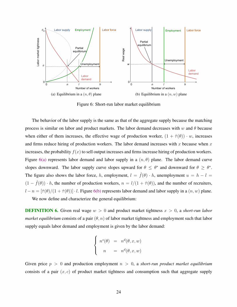
Figure 6: Short-run labor market equilibrium

The behavior of the labor supply is the same as that of the aggregate supply because the matching

process is similar on labor and product markets. The labor demand decreases with w and θ because

when either of them increases, the effective wage of production worker, (1 + τ(θ)) · w, increases

and firms reduce hiring of production workers. The labor demand increases with x because when x

increases, the probability f(x) to sell output increases and firms increase hiring of production workers.

Figure 6(a) represents labor demand and labor supply in a (n, θ) plane. The labor demand curve

slopes downward. The labor supply curve slopes upward for θ ≤ θ∗ and downward for θ ≥ θ∗.

The figure also shows the labor force, h, employment, l = f(θ) · h, unemployment u = h − l =

(1 − f(θ)) · h, the number of production workers, n = l/(1 + τ(θ)), and the number of recruiters,

l−n = [τ(θ)/(1 + τ(θ))] · l. Figure 6(b) represents labor demand and labor supply in a (n,w) plane.

We now define and characterize the general equilibrium:

DEFINITION 6. Given real wage w > 0 and product market tightness x > 0, a short-run labor

market equilibrium consists of a pair (θ, n) of labor market tightness and employment such that labor

supply equals labor demand and employment is given by the labor demand: ns(θ) = nd(θ, x, w)

n = nd(θ, x, w)

Given price p > 0 and production employment n > 0, a short-run product market equilibrium

consists of a pair (x, c) of product market tightness and consumption such that aggregate supply

24

equals aggregate demand and consumption is given by the aggregate demand: cs(x, n) = cd(x, p)

c = cd(x, p)

Given prices (p, w), a short-run general equilibrium consists of a quadruplet (x, θ, c, n) of tightnesses

and quantities such that (θ, n) is a short-run labor market equilibrium given (x,w) and (x, c) is a

short-run product market equilibrium given (n, p).

The short-run labor market and product market equilibria are partial equilibria because they take

as given the tightness and quantity in the other market. The product market equilibrium can be rep-

resented as in Figure 2 with y = a · nα. Similarly, the labor market equilibrium is represented in

Figure 6. In general equilibrium, the two partial-equilibrium systems hold simultaneously. The fol-

lowing proposition characterizes the general equilibrium:

PROPOSITION 4. For any p > 0 and w > 0, there exists a unique short-run general equilibrium

with positive consumption. The equilibrium tightnesses, (x, θ), are the unique solution to the system

h1−α · f(θ)1−α · (1 + τ(θ))α =a · αw· f(x) (13)

h · f(θ) · (1 + τ(x))ε−1 =α

w·(

χ

1− χ

)ε· µpε. (14)

Equation (13) implicitly defines θ as a strictly increasing function of x while equation (14) implicitly

defines θ as a strictly decreasing function of x. These two functions intersect exactly once.

Equation (13) arises from the partial-equilibrium condition on the labor market combining (12)

with ns(θ) =(f(θ)− ρ · θ

)· h = f(θ) · h/[1 + τ(θ)]. Equation (14) arises from a combination

of the partial-equilibrium conditions on the labor and product markets19 combining (9) with y =

f(x) · a · nα = f(θ) · h · w/α obtained from (12). Figure 7 represents the general equilibrium as

the intersection of an upward-sloping and a downward-sloping curve in a (x, θ) plane. The upward-

sloping curve is the locus of points (x, θ) that solve (13), and the downward-sloping curve is the locus

of points (x, θ) that solve (14).20

19In addition to the equilibrium with positive consumption, there exist two other equilibria with zero consumption.Appendix A extends Proposition 4 to characterize all the possible equilibria and to describe the domain and codomain ofthe functions implicitly defined by (13) and (14).

20On Figure 7, the domain of the function that solves equation (14) is [0, xm]. If the price, p, is below some threshold,the function is only defined for x above some threshold (this threshold is necessarily below xm). At the threshold, thefunction asymptotes to +∞. See Appendix A for more details.

25

Product market tightness

Labo

r mar

ket t

ight

ness

Equation (13)

θm

xm  0 0

Equation (14)

θ

x  

General equilibrium

Figure 7: Short-run general equilibrium in the model of Section 3

In our model, firms may not want to hire all the workers in the labor force even if it is costless to

hire and consumers may not want to purchase all the production even if it is costless to shop. If the

matching costs are arbitrarily small (ρ→ 0 and ρ→ 0), then τ(x)→ 0 and τ(θ)→ 0. Equations (13)

and (14) indicate that in equilibrium, f(x) < 1 and f(θ) < 1 when w and p are large enough. In that

case, some production remains unsold and some workers remain unemployed.

3.4 Efficient Allocation

DEFINITION 7. The efficient allocation is the quadruplet (x, θ, c, n) that maximizes welfare,[χ · c ε−1

ε + (1− χ) · µ ε−1ε

] εε−1

, subject to the matching frictions on the product market, c ≤ (f(x)− ρ · x)·a · nα, and to the matching frictions on the labor market, n ≤

(f(θ)− ρ · θ

)· h.

PROPOSITION 5. The efficient allocation is (x∗, θ∗, c∗, n∗), where x∗, θ∗, c∗ and n∗ are defined by

f ′(x∗) = ρ, c∗ = [f(x∗)− ρ · x∗] · y, f ′(θ∗) = ρ, and n∗ = [f(θ∗)− ρ · θ∗] · h. The real wage w∗ and

price p∗ that implement the efficient allocation are

w∗ = a · α · hα−1 ·(

1− ρη

1+η

) 1η ·(

1− ρη

1+η

)α− 1−αη

(15)

p∗ =χ

1− χ ·( µ

a · hα) 1ε ·(

1− ρη

1+η

)1− 1+ηε·η ·

(1− ρ

η1+η

)−α·(1+η)ε·η

. (16)

The economy can be in five different regimes:

DEFINITION 8. The economy is efficient if θ = θ∗ and x = x∗, labor-slack and product-slack if

θ < θ∗ and x < x∗, labor-slack and product-tight if θ < θ∗ and x > x∗, labor-tight and product-slack

if θ > θ∗ and x < x∗, labor-tight and product-tight if θ > θ∗ and x > x∗.

26

labor-slack product-tight

Pric

e Real wage

labor-slack product-slack

efficient

w*

p*

px(w)

labor-tight product-tight

p✓(w)

labor-tight product-slack

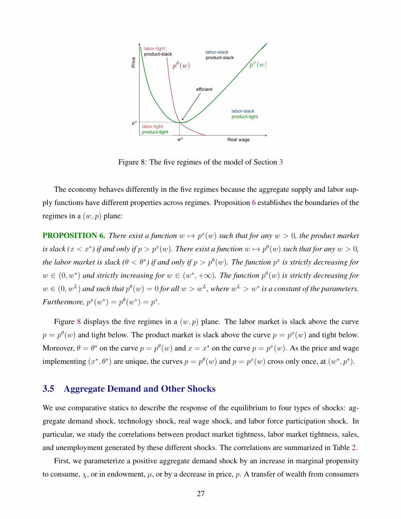
Figure 8: The five regimes of the model of Section 3

The economy behaves differently in the five regimes because the aggregate supply and labor sup-

ply functions have different properties across regimes. Proposition 6 establishes the boundaries of the

regimes in a (w, p) plane:

PROPOSITION 6. There exist a function w 7→ px(w) such that for any w > 0, the product market

is slack (x < x∗) if and only if p > px(w). There exist a function w 7→ pθ(w) such that for any w > 0,

the labor market is slack (θ < θ∗) if and only if p > pθ(w). The function px is strictly decreasing for

w ∈ (0, w∗) and strictly increasing for w ∈ (w∗,+∞). The function pθ(w) is strictly decreasing for

w ∈ (0, wL) and such that pθ(w) = 0 for all w > wL, where wL > w∗ is a constant of the parameters.

Furthermore, px(w∗) = pθ(w∗) = p∗.

Figure 8 displays the five regimes in a (w, p) plane. The labor market is slack above the curve

p = pθ(w) and tight below. The product market is slack above the curve p = px(w) and tight below.

Moreover, θ = θ∗ on the curve p = pθ(w) and x = x∗ on the curve p = px(w). As the price and wage

implementing (x∗, θ∗) are unique, the curves p = pθ(w) and p = px(w) cross only once, at (w∗, p∗).

3.5 Aggregate Demand and Other Shocks

We use comparative statics to describe the response of the equilibrium to four types of shocks: ag-

gregate demand shock, technology shock, real wage shock, and labor force participation shock. In

particular, we study the correlations between product market tightness, labor market tightness, sales,

and unemployment generated by these different shocks. The correlations are summarized in Table 2.

First, we parameterize a positive aggregate demand shock by an increase in marginal propensity

to consume, χ, or in endowment, µ, or by a decrease in price, p. A transfer of wealth from consumers

27

with low marginal propensity to consume to consumers with high marginal propensity to consume,

as in Section 2.5, would have the same effects. A positive aggregate demand shock leads to an up-

ward shift of the curve defined by equation (14) in Figure 7. After the shock, labor market tightness

and product market tightness increase. Unemployment decreases because u = h · (1 − f(θ)). Sales

increase because equation (13) implies that s = f(x) · a · nα = (w/α) · h · f(θ). The response of

consumption and employment of production workers depends on the regime. In the efficient regime,

neither consumption nor employment respond to a marginal change in tightness. Employment of pro-

duction workers decreases in a labor-tight regime but increases in a labor-slack regime. Consumption

decreases in a product-tight and labor-tight regime but increases in a product-slack and labor-slack

regime. In the two other regimes, nα and f(x)− ρ · x move in opposite direction so it is not possible

to determine the change in consumption. In the partial-equilibrium diagram of Figure 2, a positive

aggregate demand shock leads to an upward rotation of the aggregate demand curve. This rotation

raises product market tightness. In the partial-equilibrium diagram of Figure 6, the increase in product

market tightness leads to an outward shift of labor demand because the probability to sell is higher.

Labor market tightness increases as a result. Since the number of production workers changes, aggre-

gate supply adjusts in Figure 2. Product market tightness adjusts again, which feedbacks on the labor

demand. Feedbacks between labor demand and aggregate supply continue until convergence to the

new general equilibrium with higher labor market and product market tightnesses.

Second, we consider an increase in technology, a. A positive technology shock leads to an up-

ward shift of the curve defined by equation (14) in Figure 7. After the shock, labor market tightness

increases but product market tightness decreases. For the same reasons as with a positive aggre-

gate demand shock, unemployment decreases and sales increase. And as under an aggregate demand

shock, the response of consumption and employment of production workers depends on the regime.

In the partial-equilibrium diagram of Figure 2, an increase in technology leads to an expansion of

the aggregate supply curve. In the partial-equilibrium diagram of Figure 6, an increase in technology

leads to an outward shift of the labor demand curve. The resulting changes in product market tightness

and labor market tightness influence the probability to sell and employment of production workers,

which in turn feedback to the aggregate supply and labor demand curves. Feedbacks between labor

demand and aggregate supply continue until convergence to the new general equilibrium with higher

labor market tightness and lower product market tightness.

Third, we consider an increase in real wage, w. This increase leads to downward shifts of the

curves defined by equations (13) and (14) in Figure 7. After the shock, labor market tightness de-

creases and unemployment increases. On the other hand, the response of product market tightness is

28

ambiguous. We distinguish between labor-slack an labor-tight regimes. In a labor-slack regime, em-

ployment of production workers decreases when labor market tightness decreases. In the diagram of

Figure 2, the aggregate supply curve contracts whereas the aggregate demand curve remains the same.

Therefore, product market tightness, x, increases whereas consumption, given by c = cd(x, p), and

sales, given by s = (1+τ(x)) ·cd(x, p), decrease (both x 7→ cd(x, p) and x 7→ (1+τ(x)) ·cd(x, p) are

strictly decreasing). In a labor-tight regime, employment of production workers increases when labor

market tightness decreases. In the diagram of Figure 2, the aggregate supply curve expands whereas

the aggregate demand curve remains the same. Therefore, product market tightness decreases whereas

consumption and sales increase.

Finally, we consider an increase in labor force participation, h. This increase leads to downward

shifts of the curves defined by equations (13) and (14) in Figure 7. After the shock labor market

tightness, θ, decreases. Unemployment, u = h · (1− f(θ)), increases because the unemployment rate,

1−f(θ), increases and the number of workers in the labor force, h, increases. The response of product

market tightness, x, is ambiguous on the general-equilibrium diagram of Figure 7; instead, we use the

partial-equilibrium diagrams of Figures 2 and 6. Assume that x increases. Then the employment

of production workers, n = nd(θ, x, w), increases because the function nd is strictly increasing in

x and strictly decreasing in θ. Hence, the aggregate supply curve in Figure 2 expands and x falls

in equilibrium. We reach a contradiction so x decreases. As a consequence, consumption, given by

c = cd(x, p), and sales, given by s = (1 + τ(x)) · cd(x, p), increase. Finally, since s = f(x) · a · nα, s

increases, and f(x) decreases, it must be that n increases.

If we could map the variables of the model to macrodata, we could exploit the comparative-statics

results summarized in Table 2 to separate between different types of macroeconomic shocks. An ag-

gregate demand shock is the only shock under which product market tightness and sales are positively

correlated. A labor force participation shock is the only shock under which sales and unemployment

are positively correlated in a labor-slack regime (in a labor-tight regime, both labor force participa-

tion shock and real wage shock generate such a positive correlation). A technology shock is the only

shock under which product market tightness and labor market tightness are negatively correlated in a

labor-tight regime (in a labor-slack regime, both technology shock and real wage shock generate such

a negative correlation).

29

Table 2: Comparative statics in the model of Section 3

Effect on:

Increase in: Product market tightness Labor market tightness Sales Unemployment

Aggregate demand > 0 > 0 > 0 < 0

Technology < 0 > 0 > 0 < 0

Real wage > 0 if labor-slack < 0 < 0 if labor-slack > 0

< 0 if labor-tight > 0 if labor-tight

Labor force < 0 < 0 > 0 > 0

Notes: The comparative statics are derived in Section 3.5. An increase in aggregate demand results from an increase inendowment, µ, a decrease in price, p, or an increase in marginal propensity to consume, χ.

3.6 The Possibility of Reducing Unemployment by Increasing Wages

This section extends the model along two directions to improves its realism. First, we distinguish

between buyers in a long-term relationship with a firm, which we call customers, and other buyers.

This is equivalent to the usual assumption in labor market search models that some individuals are

already employed. Second, we account for inequality in labor income, wealth, and share of profits

received. With such extensions, a wage increase may reduce unemployment. With inequality and

customer-firm relationships, it is difficult to describe the set of price-wage pairs for which the general

equilibrium exists and to do comparative statics. To simplify, we assume Cobb-Douglas utility and

no matching costs. We describe the results formally in Appendix D and informally here.

We begin by deriving the aggregate supply. Each firm has κ < y customers, where y = a · nα

is the firm’s output. Each customer buys one good with certainty at price p > 0. The remaining

y − κ goods may be purchased by consumers who are not customers through the matching process.

Each consumer purchases κ goods through customer relationships and visits v firms to purchase more

goods through the matching process. The number of trades made in the matching process is s− κ =[(y − κ)−η + v−η

]− 1η . In each of these trades, a consumer buys one good at price p. The product

market tightness is x ≡ v/ [y − κ]. Let f(x) ≡ (s − κ)/(y − κ) be the probability that a firm sells

one good to a buyer who is not a customer. The probability f(x) satisfies (1). The matching cost, ρ,

is zero so consumption equals purchases. Accordingly, the aggregate supply is given by

cs(x, n) = κ+ f(x) · (a · nα − κ) . (17)

Next, we derive the aggregate demand. Workers belong to one of G groups of measure 1/G.

30

Group g’s per person utility is given by (10). Group g’s per person budget is

mg + p · cg = µg + σg · Π +$g · p · w · n,

where σg is group g’s per person share of profits, Π are nominal profits, and $g is group g’s per

person share of labor income. By construction,(∑

g σg

)/G = 1 and

(∑g$g

)/G = 1. The

optimal consumption of produced good, cg, is related to the optimal consumption of nonproduced

good, mg, by a relationship similar to (5) with ε = 1. Substituting out profits from group g’s income

using Π = p · [κ+ f(x) · (y − κ)− w · n], we find that group g’s optimal consumption satisfies

p · cg = χg · {µg + σg · p · [κ+ f(x) · (y − κ)] + ($g − σg) · p · w · n}

We define aggregate demand as the sum of each group’s demand: cd ≡(∑

g cg

)/G. In equilibrium,

purchases equal sales:(∑

g cg

)/G = κ+ f(x) · (y − κ). Thus, aggregate demand is given by

cd(n, p, w) =1

p·

∑g µg · χg∑

g(1− χg) · σg+

∑g χg · ($g − σg)∑g(1− χg) · σg

· w · n. (18)

Aggregate demand does not depend on product market tightness because the matching wedge, τ(x),

is zero. If profits and labor income are uniformly distributed across group such that σg = $g = 1

for all g, aggregate demand depends only on the price, p, groups’ endowments, {µg}, and groups’

preferences, {χg}. If profits or labor income are not uniformly distributed across group such that∑g χg · ($g − σg) 6= 0, aggregate demand also depends on the wage bill, w · n. A wage increase

stimulates aggregate demand if

∑g

χg ·$g >∑g

χg · σg. (19)

This condition says that across groups, the correlation between share of labor income and marginal

propensity to consume is higher than the correlation between share of profits and marginal propensity

to consume. Loosely speaking, wage earners have a higher marginal propensity to consume than firm

owners; alternatively, profits are more concentrated among savers than labor income. A wage in-

crease always redistributes income from firm owners to wage earners. If (19) holds, this redistribution

stimulates aggregate demand.

The labor market is the same as above and the marginal decisions of firms are not affected by the

31

presence of customers; hence, labor demand and labor supply satisfy Definition 5. Aggregate supply

and aggregate demand satisfy (17) and (18). A short-run general equilibrium satisfies Definition 6. A

major difference with the results from Proposition 4 is that a general equilibrium does not exist for all

parameter values and all price-wage pairs. But when a general equilibrium with positive consumption

and employment exists, it is unique and we can perform comparative statics.

We identify conditions on parameter values such that a wage increase reduces unemployment.

Condition (19) is necessary because it ensures that a wage increase stimulates aggregate demand.

Another necessary condition is[∑

g µg · χg]/[∑

g(1− χg) · σg]< κ, which requires the customer

base κ to be positive. Under this condition the labor-income component of aggregate demand tends

to be large relative to the endowment component, and a wage increase tends to have a large positive

effect on aggregate demand.

In fact, a wage increase has two opposite effects. First, a wage increase raises the marginal cost

of labor and depresses labor demand. This is the conventional effect, which is found in all matching

models of the labor market. Second, a wage increase redistributes income from firm owners to wage

earners. This redistribution stimulates aggregate demand if wage earners have a higher marginal

propensity to consumer than firm owners. An increase in aggregate demand leads to higher product

market tightness, which stimulates labor demand. This is an unconventional effect, which arises in

our model only in presence of a frictional product market and inequality. A wage increase lowers

unemployment when the unconventional positive response of aggregate demand to the wage increase

is strong enough to dominate the conventional negative response of labor demand.

The result that a wage increase may decrease unemployment has a number of implications. One

implication is that the effect of the minimum wage on employment may be different in partial equi-

librium and in general equilibrium. In partial equilibrium the influence of the minimum wage on

aggregate demand is omitted. In general equilibrium the influence of the minimum wage on aggre-

gate demand is accounted for. Increasing the minimum wage necessarily depresses employment in

partial equilibrium, but when (19) holds, the disemployment effect of the minimum wage is not as

strong in general equilibrium as in partial equilibrium. Under stronger conditions, the minimum wage

may have a negative employment effect in partial equilibrium but a positive employment effect in

general equilibrium.21 One possible reason why empirical studies estimating the employment effect

of the minimum wage reach conflicting conclusions is that these studies do not distinguish between

21This discussion parallels the comparison of the microelasticity and macroelasticity of unemployment with respect tounemployment insurance in Landais, Michaillat and Saez [2010].

32

partial- and general-equilibrium effects.22 On the one hand, studies measuring employment effects

within a labor market, for example by comparing workers eligible for the minimum wage to workers

ineligible, estimate partial-equilibrium effects. On the other hand, studies measuring employment

effects across labor markets estimate general-equilibrium effects. If (19) held, the within-state studies

would systematically estimate larger disemployment effect than the cross-state studies.

4 Relation to Other Macroeconomic Models

In this section, we argue that our matching framework is not restrictive. With alternative assumptions

about the functional forms of the utility, production, and matching functions, the value of matching

costs, and the price and wage schedules, our framework can replicate the key first-order conditions

of a broad range of macroeconomic models—perfect-competition model, existing matching models,

fixprice-fixwage model, and monopolistic-competition model. We then explain why making these

alternative assumptions would eliminate aggregate demand effects captured by our model.

4.1 Perfect-Competition Model

Assume that the matching costs, ρ and ρ, are zero. Assume that the real wage equals the marginal

product of the last worker in the labor force and that the price equals the marginal rate of substitution

between the produced good and the nonproduced good at full employment:

w = a · α · hα−1 (20)

p =χ

1− χ ·( µ

a · hα) 1ε. (21)

Under these assumptions, equation (14) implies that

f(θ) =1

h· α

a · α · hα−1 ·(

χ

1− χ

)ε· µ ·

(χ

1− χ

)−ε·(a · hαµ

)= 1.

Thus, θ → +∞ and n = f(θ) · h = h. Equation (13) implies that

f(x) =a · α · hα−1

a · α · h1−α = 1.

22For a survey of the vast empirical literature on the minimum wage, see for instance Card and Krueger [1995].

33

Thus, x → +∞ and c = f(x) · a · hα = a · hα. Labor and product markets behave as if they were

perfectly competitive. The matching wedges are zero: τ(x) = τ(θ) = 0. Firms sell all of their

production at the going price: f(x) = 1. All labor force participants find a job at the going wage:

f(θ) = 1. There is no unemployment: n = h. There is no unsold production: c = a · hα.

These assumptions are inadequate to study aggregate demand because they eliminate all the effects

from aggregate demand shocks. Indeed, employment and consumption do not depend on aggregate

demand: n = h and c = a · hα for any value µ of endowment and any value χ of the marginal

propensity to consume. Aggregate demand shocks have no effect because any shock to the marginal

propensity to consume, χ, or the endowment, µ, is absorbed by a corresponding change in price, p,

such that the aggregate demand, cd = [χ/(1− χ)]ε · (µ/pε), does not change.

4.2 Other Matching Models

The following assumptions capture the main features of existing matching models with a product

market and a labor market. We assume that consumers have a linear utility function, which is the

special case of the CES utility function when ε → +∞, and that firms have a linear production

function, which is the special case of our production function when α = 1. The optimal consumption

choice of consumers, given by (5), and the optimal employment choice of firms, given by (12), yield

(1 + τ(x)) · p =χ

1− χ (22)

(1 + τ(θ)) · w = a · f(x). (23)

Equations (22) and (23) show that tightnesses are pinned down independently of quantities so that

both aggregate demand and labor demand are perfectly elastic with respect to x and θ respectively.

The diagrams of Figure 9 represent the product market in a (c, x) plane and the labor market in a

(n, θ) plane. Both aggregate demand and labor demand are represented by horizontal curves.

Existing matching models assume either that price and wage are the outcome of bargaining, or

that price and wage are rigid.23 In a bargaining model, real wage and price are given by

w = β · a · f(x) (24)

p = β · χ

1− χ, (25)

23See Wasmer [2011] for a model assuming bargaining and Hall [2008] for a model assuming rigid price and wage.

34

Aggregate demand

Quantity of product

0

Pro

duct

mar

ket t

ight

ness

0

Aggregate supply xm Output

c

x

s

Sales

y

Partial equilibrium

(a) Partial equilibrium on the product markett Number of workers

0

Labo

r mar

ket t

ight

ness

0

Labor supply θm

Partial equilibrium

Labor demand

n

θ

l

Employment

h

Labor force

(b) Partial equilibrium on the labor market

Figure 9: The matching model with linear utility function and linear production function

where β ∈ (0, 1) and β ∈ (0, 1) are parameters. The real wage is the generalized Nash solution of

the bargaining problem between a worker and a firm when the worker has bargaining power β. The

surplus to the firm of hiring one worker is F(w) = a · f(x)− w. The surplus to the worker of being

hired is W(w) = w. The Nash solution maximizes F(w)1−β · W(w)β , so W(w) = β · [W(w) +

F(w)] = β · a · f(x) and w satisfies (24). The price is the generalized Nash solution to the bargaining

problem between a consumer and a firm when the firm has bargaining power β. The surplus to the

consumer of buying one unit of produced good is C(p) = χ− p · (1− χ). The surplus to the firm of

selling one unit of produced good is F(p) = p · (1 − χ). Firms are owned by consumers so firms’

marginal income is valued at consumers’ marginal utility of consumption of nonproduced good. The

Nash solution maximizes C(p)1−β · F(p)β , so F(p) = β · [F(p) + C(p)] = β · χ and p satisfies (25).

Combining (22), (23), (24) and (25), we determine the equilibrium tightnesses:

β · (1 + τ(x)) = 1 and β · (1 + τ(θ)) = 1.

Hence both x and θ are pinned down independently of quantities hereby eliminating all the effects

from aggregate demand shocks. Indeed, employment and consumption are given by the supply equa-

tions n = ns(θ) and c = cs(x, n) and are independent of the aggregate demand parameters, µ and χ.

Aggregate demand shocks are eliminated because the bargained price is proportional to the marginal

rate of substitution between produced good and nonproduced good, χ/(1− χ).

Instead of assuming price and wage bargaining, assume instead that price and real wage are pa-

rameters of the model as in Hall [2008]. For the equilibrium to exist, it is necessary that p < χ/(1−χ)

35

and w < a. The equilibrium tightnesses are given by (22) and (23). Since price and wage are rigid,

aggregate demand shocks (shocks to χ) affect equilibrium tightnesses and quantities. However, many

elements of our analysis disappear in this model because the demand curves are perfectly elastic: the

transfers of Section 2.5 have no effect because wealth plays no role; the government-purchase multi-

plier of Section 2.6 is always zero; unemployment and unsold production would disappear in absence

of matching costs, irrespective of the level of aggregate demand or labor demand.

4.3 Monopolistic-Competition Model

We begin by presenting a model with monopolistic competition on the product market and labor

market. The model is a variant of the model of Blanchard and Kiyotaki [1987, Section 2]. Since

this model is standard, we omit derivations and only report equilibrium conditions. The economy is

composed of a continuum of firms indexed by i ∈ [0, 1] and a continuum of households indexed by

j ∈ [0, 1]. The goods produced by firms are imperfect substitutes and the types of labor supplied by

households are also imperfect substitutes, so firms and households have some monopoly power.

The utility function of household j is given by

χ · ln(cj) + (1− χ) · ln(mj)− ν ·ξ

1 + ξ· n

1+ξξ

j . (26)

Utility depends on consumption of nonproduced good, mj , number of hours worked, nj ∈ (0, 1), and

a consumption index, cj ≡(∫ 1

0cζ−1ζ

ij di

) ζζ−1

, where cij is consumption of good i. The parameters

ν > 0, ξ > 0, and ζ > 1, measure the disutility from labor, the curvature of the disutility for labor,

and the elasticity of substitution between goods in utility. The budget constraint of household j is

mj +

∫ 1

0

pi · cijdi = µj +Wj · nj + Πj, (27)

where pi is the price of good i, Wj is the nominal wage for labor of type j, Πj is the share of aggregate

profits distributed to the household, and µj > 0 is the endowment received by the household. The

aggregate endowment of nonproduced good is µ =∫ 1

0µjdj. Given {pi}, household j chooses {cij},

mj , nj , and Wj to maximize (26) subject to (27) and to a demand schedule for its labor, a decreasing

function of Wj arising from firms’ profit maximization.

36

Firm i hires labor to produce output. Its production function is

ci = a ·(∫ 1

0

nγ−1γ

ij dj

)α· γγ−1

, (28)

where ci is output of good i, a is the technology level, nij is the number of workers of type j hired,

γ > 1 is the elasticity of substitution between types of labor in production, and α < 1 indicates

decreasing returns to scale. Given {Wj}, firm i chooses {nij}, ci and pi to maximize profits

pi · ci −∫ 1

0

Wj · nijdj.

subject to (28) and to a demand schedule for its good, a decreasing function of pi arising from house-

holds’ utility maximization.

In the symmetric general equilibrium, all households and firms are identical, they set the same

prices and wages, and they produce and work the same amounts. In this equilibrium, we have

W

p=

γ

γ − 1· ν · n 1

ξ · cχ

(29)

p

W=

ζ

ζ − 1· 1

α · a · n1−α, (30)

whereW is the nominal wage paid by all firms, p is the price charged by all firms, and n and cmeasure

the aggregate number of hours worked and aggregate quantity of goods produced. Equation (29) says

that households set the real wage at a markup γ/(γ − 1) > 1 over its marginal rate of substitution

between leisure and consumption. Equation (30) says that firms set the price at a markup ζ/(ζ−1) > 1

over the marginal cost of producing one item.

Our matching model generates the same markups as the model with monopolistic competition

under appropriate assumptions. Assume that matching costs are zero and that consumers have a

utility function given by χ · ln(c) + (1 − χ) · ln(m) − ν · [ξ/ (1 + ξ)] · h1+ξξ , where h is the number

of workers in the labor force searching for a job. Given that h = n/f(θ), the optimal choice of labor

force participation imposes

W

p=

1

f(θ)1+ξξ

· ν · n 1ξ · cχ,

37

where W ≡ w · p is the nominal wage. With ρ = 0 and hence τ(θ) = 0, equation (12) becomes

p

W=

1

f(x)· 1

α · a · n1−α.

We make two assumptions on tightnesses to close the model:

f(x) =ζ − 1

ζ(31)

f(θ) =

(γ − 1

γ

) ξ1+ξ

. (32)

These assumptions impose that the job-finding probability is the inverse of the labor market markup

and the selling probability is the inverse of the product market markup to the power of ξ/(1+ξ). Under

these conditions, the quadruplet (c, n,W, p) satisfies equations (29) and (30) both in the model with

matching frictions and in the model with monopolistic competition. The ratio between the marginal

product of labor and the marginal rate of substitution, sometimes called the labor wedge, is therefore

identical in the two models and equal to γ · ξ/ [(γ − 1) · (ξ − 1)] > 1.

These assumptions are inadequate to study aggregate demand because they eliminate all the effects

from aggregate demand shocks. Indeed, unemployment rate and consumption do not depend on

aggregate demand: u =(

1− f(θ))· h and c = f(x) · a · f(θ)α · hα where f(x) and f(θ) depend

only on the parameters ζ , γ, and ξ and not on the parameters capturing aggregate demand, µ and

χ. Aggregate demand shocks have no effect because the price always adjusts such that (31) holds.

Given that f(x) and the real wage remain the same, the labor demand does not respond to aggregate

demand shocks. The labor supply does not respond either so unemployment is unaffected. In fact,

the price response is such that the aggregate demand curve does not shift in response to aggregate

demand shocks. Aggregate demand shocks impact unemployment in this model only if (31) and (32)

do not always hold. One way to eliminate (31) and (32) is to assume instead that price and real wage

are somewhat rigid, which brings us back to the model of Section 3.24

4.4 Fixprice-Fixwage Model

The standard fixprice-fixwage model was developed by Barro and Grossman [1971].25 Our model

cannot replicate the allocation of that model because firms’ sales are sometimes determined by a

24This is only a reinterpretation of the insight of Blanchard and Kiyotaki [1987]. They showed that aggregate demandshocks have effects in the monopolistic-competition model only if prices are rigid.

25See Benassy [1993] for an overview of this class of models and their properties.

38

demand constraint in that model whereas they are always determined by a marginal decision in our

model.26 Our model can, however, replicate the allocation of a fixprice-fixwage model with a propor-

tional rationing rule. With this rule, all agents on the rationed side of the market trade with the same

probability. This alternative model predicts slightly different allocations from the standard fixprice-

fixwage model, but the allocations can still be sorted into its four traditional regimes.

To replicate the allocation of the fixprice-fixwage model with proportional rationing, we assume

that the matching costs are zero and that the matching functions are given by s = min {v, y} and

l = min {v, h}. These matching functions are the special case of those considered in our model when

η → +∞ and η → +∞. Since the matching functions have a kink, the matching probabilities have

a kink as well: f(x) = min {x, 1} and f(θ) = min {θ, 1}. Accordingly, the supply functions are

defined piecewise, with one piece when the relevant tightness is below 1 and one piece when it is

above 1: ns(θ) = min {θ, 1} · h and cs(x, n) = min {x, 1} · a · nα. Since the matching wedges, τ(x)

and τ(θ), are zero, the demand functions do not depend on the tightness in their market: nd(θ, x, w) =

(min {x, 1} · a · α/w)1

1−α and cd(p) = [χ/ (1− χ)]ε · µ/pε. In particular, equilibrium consumption

is c = [χ/ (1− χ)]ε · µ/pε. Supply and demand curves are represented in Figure 10 in a (c, x) plane

and in a (n, θ) plane. The aggregate supply and labor supply are piecewise linear with a kink at

x = 1 and θ = 1, respectively; the aggregate demand is vertical; and the labor demand is vertical.

Given price and real wage, tightnesses and quantities are determined by the intersection of supply

and demand curves. By introducing matching functions that govern the number of trades on each

market, we rewrite the fixprice-fixwage model, which traditionally is a disequilibrium model, as an

equilibrium model. Before describing the four regimes, we define two functions to help delimitate

them: p 7→ wθ(p) = (α/h) · [χ/ (1− χ)]ε ·µ/pε and p 7→ wx(p) = α · a 1α · {[(1− χ) /χ]ε · pε/µ}

1−αα .

The function wθ decreases from +∞ to 0 for p ∈ (0,+∞). The function wx increases from 0 to +∞for p ∈ (0,+∞). Accordingly, the equation wθ(p) = wx(p) admits a unique solution on (0,+∞),

which we denote p∗. We denote w∗ = wθ(p∗). We can show that p∗ is given by (21) and w∗ is given

by (20). Figure 10(c) delimitates the four regimes in a (p, w) plane.

In the Keynesian unemployment regime, there is excess supply in the labor and product market:

26Indeed when demand is low in the standard fixprice-fixwage model, firms sell all of their output up to a fixed numberof items and none above that number. In our model, firms sell all their output with the same probability; they chooseoutput and thus sales to equalize marginal cost with marginal revenue.

39

1 > f(θ) = θ and 1 > f(x) = x. The equilibrium tightnesses satisfy

θ =α

h · w ·(

χ

1− χ

)ε· µpε

x =wα

a · αα ·[(

χ

1− χ

)ε· µpε

]1−α.

Employment n = θ · h is determined partly by aggregate demand and partly by the real wage. In

the standard fixprice-fixwage model, employment only depends on demand in the Keynesian unem-

ployment regime. In our model, employment also depends on the wage because firms have a positive

probability to sell any amount of production so employment is determined by the marginal cost of

labor and not by a quantity constraint. This regime prevails if w > wθ(p) and w < wx(p). In the

classical unemployment regime, there is excess supply in the labor market and excess demand in the

product market: 1 > f(θ) = θ and 1 = f(x). Product market tightness x ≥ 1 is irrelevant. Labor

market tightness satisfies

θ =1

h·(α · aw

) 11−α

.

Employment n = θ · h is completely determined by the real wage. Aggregate demand does not

matter because firms sell all their production for sure on the product market. This regime prevails if

w > w∗ and w = wx(p). If w > wx(p), there is no equilibrium. In the underconsumption regime,

there is excess demand in the labor market and excess supply in the product market: f(θ) = 1 and

1 > f(x) = x. Labor market tightness θ ≥ 1 is irrelevant. Product market tightness satisfies

x =w

a · α · hα−1 .

There is no unemployment: n = h. This regime prevails if w < w∗ and w = wθ(p). If w < wθ(p),

there is no equilibrium. In the repressed inflation regime, there is excess demand in the labor market

and excess demand in the product market: f(θ) = 1 and f(x) = 1. The tightnesses x ≥ 1 and θ ≥ 1

are irrelevant. There is no unemployment: n = h. This regime prevails for w = w∗ and p = p∗. Price

and real wage are exactly the same as in the perfectly competitive case. Thus, the repressed inflation

regime is identical to the Walrasian equilibrium.

The assumptions made in this section could be used to study the effect of aggregate demand on

unemployment. However, these assumptions limit the theory without clear advantages. First, the

equilibrium is not well defined for all positive prices and wages. Second, the theory is complex

40

0 0

1

Aggregate demand

c

Unsold production

Aggregate supply P

rodu

ct m

arke

t tig

htne

ss

x

Quantity of product y

Output

(a) Excess demand in the product market

Number of workers

0

Labo

r mar

ket t

ight

ness

0

Labor supply

1

Labor demand

h n

θ

Unemployment

Labor force

(b) Excess demand in the labor market

Price

Rea

l wag

e

Repressed inflation

w✓(p) wx(p)

Keynesian unemployment

Classical unemployment

Underconsumption

p⇤

w⇤

(c) The four regimes of the fixprice-fixwage model

Figure 10: The fixprice-fixwage model of Section 4.4

because it requires to determine in which of the four regimes the economy operates in order to know

which equilibrium conditions hold. Third, aggregate demand plays an interesting role only in the

Keynesian unemployment regime, and not in the other regimes.

5 Conclusion

This paper proposes a parsimonious model that links unemployment to aggregate demand. We en-

vision three applications for the model. First, the model could be used to analyse the impact on

unemployment of a broad range of fiscal policies that affect simultaneously aggregate demand, labor

demand, and labor supply. The model could address the following questions: Should unemployment

insurance be more generous in recessions to stimulate aggregate demand, or should it be less generous

to incentivize jobseekers to search more? Should payroll tax shift from employees to employers in

41

recessions to stimulate aggregate demand, or should it shift from employers to employees to reduce

labor cost and stimulate hiring? Should the minimum wage rise in recessions to increase the income

of poorer workers with a high marginal propensity to consume and thus stimulate aggregate demand,

or should it fall to stimulate hiring of low-income workers? Should income tax be more progressive

in recessions to stimulate aggregate demand, or should it be more regressive to encourage work?

Second, empirical research could exploit the theoretical predictions of the model to identify the

macroeconomic shocks driving business cycle fluctuations. A key result of our analysis is that product

market tightness and sales are positively correlated under aggregate demand shocks, whereas they are

negatively correlated under other shocks. This result implies that the probability to sell goods is

procyclical under aggregate demand shocks and countercyclical under other shocks. This probability

can be measured by the ratio of sales to stock for sales in a given period. Hence, empirical research

on the cyclical behavior of sales and inventories could be useful to separate between different types

of macroeconomic shocks. For instance, Bils and Kahn [2000] study empirically the cyclicality of

the ratio of sales to stock for sales in the manufacturing sector in the US. They find that this ratio is

strongly procyclical, suggesting that aggregate demand shocks play an important role in their data.

Third, the model could be a starting point to build a more sophisticated dynamic stochastic general

equilibrium model featuring unsold production and unemployment. An important restriction of the

theory, however, needs to be addressed to obtain a quantitatively realistic macroeconomic model.

The restriction is that prices are completely rigid in the short-run in response to a shock and that all

adjustments take place through tightnesses. Naturally in the long-run, market forces could push prices

to adjust if their level is inefficient. For instance if prices are too high, new markets may be created

with lower prices but higher tightness.27 Sellers and buyers have incentives to move to these new

markets because they are more efficient so there is a larger surplus to share. Sellers are compensated

for the lower price with a higher probability to sell. Buyers are compensated for the higher matching

wedge by a lower price. A mechanism that could lead to the creation of these new markets and

dynamic price adjustments in the medium-run is the competitive search mechanism of Moen [1997].

Modeling these market forces would provide a microfoundation for the aggregate supply curve of

the traditional AS-AD model; indeed, the AS curve represents the price increase arising when the

economy is overheating and the price decrease arising when the economy is slack.

27Lazear [2010] finds evidence of such behavior for price and tightness in the housing market in the US.

42

ReferencesBai, Yan, Jose-Victor Rios-Rull, and Kjetil Storesletten. 2012. “Demand Shocks as Productivity Shocks.”

http://www.econ.umn.edu/∼vr0j/papers/brs Sept 27 2012.pdf.

Barro, Robert J., and Herschel I. Grossman. 1971. “A General Disequilibrium Model of Income and Em-ployment.” American Economic Review, 61(1): 82–93.

Benassy, Jean-Pascal. 1993. “Nonclearing Markets: Microeconomic Concepts and Macroeconomic Applica-tions.” Journal of Economic Literature, 31(2): 732–761.

Bils, Mark J., and James A. Kahn. 2000. “What Inventory Behavior Tells Us about Business Cycles.” Amer-ican Economic Review, 90(3): 458–481.

Blanchard, Olivier J., and Jordi Galı. 2010. “Labor Markets and Monetary Policy: A New-Keynesian Modelwith Unemployment.” American Economic Journal: Macroeconomics, 2(2): 1–30.

Blanchard, Olivier J., and Nobuhiro Kiyotaki. 1987. “Monopolistic Competition and the Effects of Aggre-gate Demand.” American Economic Review, 77(4): 647–666.

Burdett, Kenneth, and Kenneth L. Judd. 1983. “Equilibrium Price Dispersion.” Econometrica, 51(4): 955–969.

Card, David, and Alan B. Krueger. 1995. Myth and Measurement: The New Economics of the MinimumWage. Princeton University Press.

den Haan, Wouter J., Garey Ramey, and Joel Watson. 2000. “Job Destruction and Propagation of Shocks.”American Economic Review, 90(3): 482–498.

Diamond, Peter A. 1982. “Wage Determination and Efficiency in Search Equilibrium.” Review of EconomicStudies, 49(2): 217–227.

Edgeworth, Francis Y. 1881. Mathematical Psychics: An Essay on the Application of Mathematics to theMoral Sciences. London:Kegan Paul.

Eggertsson, Gauti B., and Paul Krugman. 2012. “Debt, Deleveraging, and the Liquidity Trap: A Fisher-Minsky-Koo approach.” Quarterly Journal of Economics, 127(3): 1469–1513.

Farmer, Roger E. A. 2008. “Aggregate Demand and Supply.” International Journal of Economic Theory,4(1): 77–93.

Farmer, Roger E.A. 2009. “Confidence, Crashes and Animal Spirits.” National Bureau of Economic ResearchWorking Paper 14846.

Hall, Robert E. 2005. “ Employment Fluctuations with Equilibrium Wage Stickiness.” American EconomicReview, 95(1): 50–65.

Hall, Robert E. 2008. “General Equilibrium with Customer Relationships: A Dynamic Analysis of Rent-Seeking.” http://www.stanford.edu/∼rehall/GECR no derivs.pdf.

Hart, Oliver. 1982. “A Model of Imperfect Competition with Keynesian Features.” Quarterly Journal of Eco-nomics, 97(1): 109–138.

Heathcote, Jonathan, and Fabrizio Perri. 2012. “Wealth and Volatility.”

Hicks, John. 1965. Capital and Growth. Oxford University Press.

Howitt, Peter, and R. Preston McAfee. 1987. “Costly Search and Recruiting.” International Economic Review,28(1): 89–107.

Kaplan, Greg, and Guido Menzio. 2013. “Shopping Externalities and Self-Fulfilling Unemployment Fluctu-ations.” National Bureau of Economic Research Working Paper 18777.

Keynes, John Maynard. 1936. The General Theory of Employment, Interest and Money. Macmillan.

Landais, Camille, Pascal Michaillat, and Emmanuel Saez. 2010. “Optimal Unemployment Insurance over

43

the Business Cycle.” National Bureau of Economic Research Working Paper 16526.

Lazear, Edward P. 2010. “Why Do Inventories Rise When Demand Falls in Housing and Other Markets?”National Bureau of Economic Research Working Paper 15878.

Lehmann, Etienne, and Bruno Van der Linden. 2010. “Search Frictions on Product and Labor Markets:Money in the Matching Function.” Macroeconomic Dynamics, 14(01): 56–92.

Lorenzoni, Guido. 2009. “A Theory of Demand Shocks.” American Economic Review, 99(5): 2050–2084.

Mian, Atif, and Amir Sufi. 2012. “What Explains High Unemployment? The Aggregate Demand Channel.”Chicago Booth Working Paper 13-43.

Michaillat, Pascal. 2012. “Do Matching Frictions Explain Unemployment? Not in Bad Times.” AmericanEconomic Review, 102(4): 1721–1750.

Michaillat, Pascal. forthcoming. “A Theory of Countercyclical Government Multiplier.” American EconomicJournal: Macroeconomics.

Moen, Espen R. 1997. “Competitive Search Equilibrium.” Journal of Political Economy, 105(2): 385–411.

Montgomery, James D. 1991. “Equilibrium Wage Dispersion and Interindustry Wage Differentials.” QuarterlyJournal of Economics, 106(1): 163–179.

Mortensen, Dale T. 1982. “Property Rights and Efficiency in Mating, Racing, and Related Games.” AmericanEconomic Review, 72(5): 968–979.

Petrongolo, Barbara, and Christopher A. Pissarides. 2001. “Looking into the Black Box: A Survey of theMatching Function.” Journal of Economic Literature, 39(2): 390–431.

Pissarides, Christopher A. 1985. “Short-Run Equilibrium Dynamics of Unemployment, Vacancies, and RealWages.” American Economic Review, 75(4): 676–690.

Ramey, Valerie A. 2011. “Can Government Purchases Stimulate the Economy?” Journal of Economic Litera-ture, 49: 673–685.

Rendhal, Pontus. 2012. “Fiscal Policy in an Unemployment Crisis.” sites.google.com/site/pontusrendahl/stimulus.pdf.

Rogerson, Richard, Robert Shimer, and Randall Wright. 2005. “Search-Theoretic Models of the LaborMarket: A Survey.” Journal of Economic Literature, 43(4): 959–988.

Shimer, Robert. 2010. Labor Markets and Business Cycles. Princeton, NJ:Princeton University Press.

Wasmer, Etienne. 2011. “A Steady-State Model of Non-Walrasian Economy with Three Imperfect Markets.”http://econ.sciences-po.fr/sites/default/files/file/ewasmer/WasmerNequal3-3June2011.pdf.

44

Appendix

A ProofsWe start by proving a lemma that we use repeatedly in the proofs. The lemma characterizes thematching probabilities, defined by q(x) = (1 + xη)−

1η and f(x) = (1 + x−η)−

1η , the matching wedge,

defined by τ(x) = ρ/(q(x)−ρ), and the tightnesses xm and x∗, defined by f ′(x∗) = ρ and q(xm) = ρ.

LEMMA A1. The functions f , q, and τ and the values xm and x∗ satisfy the following properties:

• xm = (ρ−η − 1)1η

• f(xm) = (1− ρη) 1η .

• τ(xm) = +∞ and 1/(1 + τ(xm)) = 0.

• x∗ =(ρ−

η1+η − 1

) 1η

• q(x∗) = ρ1

1+η .

• f(x∗) =(

1− ρη

1+η

) 1η.

• τ(x∗) = 1/(ρ−

η1+η − 1

)and 1/(1 + τ(x∗)) = 1− ρ

η1+η .

• f(0) = 0 and limx→+∞ f(x) = 1.

• f is positive, smooth, and strictly increasing on [0,+∞).

• q(0) = 1 and limx→+∞ q(x) = 0.

• q is positive, smooth, and strictly decreasing on [0,+∞).

• τ(0) = ρ/(1− ρ) and limx→xm τ(x) = +∞.

• τ is positive, smooth, and strictly increasing on [0, xm).

• f(x) = q(x) · x.

• q′(x) = −q(x)1+η · xη−1.

• f ′(x) = q(x)1+η.

Proof. The results follow from simple algebra.

A.1 Proof of Lemma 1The proof follows directly from the definitions of x∗ and c∗, and from Lemma A1.

45

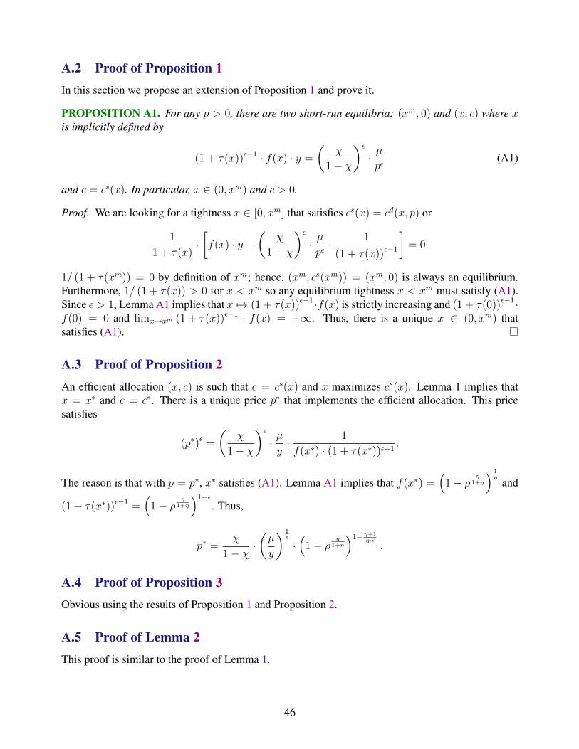
A.2 Proof of Proposition 1In this section we propose an extension of Proposition 1 and prove it.

PROPOSITION A1. For any p > 0, there are two short-run equilibria: (xm, 0) and (x, c) where xis implicitly defined by

(1 + τ(x))ε−1 · f(x) · y =

(χ

1− χ

)ε· µpε

(A1)

and c = cs(x). In particular, x ∈ (0, xm) and c > 0.

Proof. We are looking for a tightness x ∈ [0, xm] that satisfies cs(x) = cd(x, p) or

1

1 + τ(x)·[f(x) · y −

(χ

1− χ

)ε· µpε· 1

(1 + τ(x))ε−1

]= 0.

1/ (1 + τ(xm)) = 0 by definition of xm; hence, (xm, cs(xm)) = (xm, 0) is always an equilibrium.Furthermore, 1/ (1 + τ(x)) > 0 for x < xm so any equilibrium tightness x < xm must satisfy (A1).Since ε > 1, Lemma A1 implies that x 7→ (1 + τ(x))ε−1 ·f(x) is strictly increasing and (1 + τ(0))ε−1 ·f(0) = 0 and limx→xm (1 + τ(x))ε−1 · f(x) = +∞. Thus, there is a unique x ∈ (0, xm) thatsatisfies (A1).

A.3 Proof of Proposition 2An efficient allocation (x, c) is such that c = cs(x) and x maximizes cs(x). Lemma 1 implies thatx = x∗ and c = c∗. There is a unique price p∗ that implements the efficient allocation. This pricesatisfies

(p∗)ε =

(χ

1− χ

)ε· µy· 1

f(x∗) · (1 + τ(x∗))ε−1.

The reason is that with p = p∗, x∗ satisfies (A1). Lemma A1 implies that f(x∗) =(

1− ρη

1+η

) 1η

and

(1 + τ(x∗))ε−1 =(

1− ρη

1+η

)1−ε. Thus,

p∗ =χ

1− χ ·(µ

y

) 1ε

·(

1− ρη

1+η

)1− η+1η·ε.

A.4 Proof of Proposition 3Obvious using the results of Proposition 1 and Proposition 2.

A.5 Proof of Lemma 2This proof is similar to the proof of Lemma 1.

46

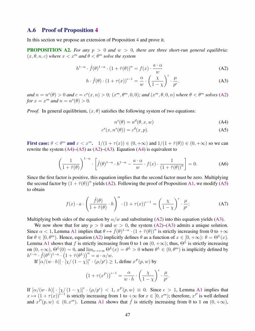
A.6 Proof of Proposition 4In this section we propose an extension of Proposition 4 and prove it.

PROPOSITION A2. For any p > 0 and w > 0, there are three short-run general equilibria:(x, θ, n, c) where x < xm and θ < θm solve the system

h1−α · f(θ)1−α · (1 + τ(θ))α = f(x) · a · αw

(A2)

h · f(θ) · (1 + τ(x))ε−1 =α

w·(

χ

1− χ

)ε· µpε. (A3)

and n = ns(θ) > 0 and c = cs(x, n) > 0; (xm, θm, 0, 0); and (xm, θ, 0, n) where θ < θm solves (A2)for x = xm and n = ns(θ) > 0.

Proof. In general equilibrium, (x, θ) satisfies the following system of two equations:

ns(θ) = nd(θ, x, w) (A4)

cs(x, ns(θ)) = cd(x, p). (A5)

First case: θ < θm and x < xm. 1/(1 + τ(x)) ∈ (0,+∞) and 1/(1 + τ(θ)) ∈ (0,+∞) so we canrewrite the system (A4)–(A5) as (A2)–(A3). Equation (A4) is equivalent to(

1

1 + τ(θ)

)1−α

·[f(θ)1−α · h1−α − a · α

w· f(x) · 1

(1 + τ(θ))α

]= 0. (A6)

Since the first factor is positive, this equation implies that the second factor must be zero. Multiplyingthe second factor by (1 + τ(θ))α yields (A2). Following the proof of Proposition A1, we modify (A5)to obtain

f(x) · a ·(

f(θ)

1 + τ(θ)· h)α

· (1 + τ(x))ε−1 =

(χ

1− χ

)ε· µpε

; (A7)

Multiplying both sides of the equation by α/w and substituting (A2) into this equation yields (A3).We now show that for any p > 0 and w > 0, the system (A2)–(A3) admits a unique solution.

Since α < 1, Lemma A1 implies that θ 7→ f(θ)1−α · (1 + τ(θ))α is strictly increasing from 0 to +∞for θ ∈ [0, θm). Hence, equation (A2) implicitly defines θ as a function of x ∈ [0,+∞): θ = ΘL(x).Lemma A1 shows that f is strictly increasing from 0 to 1 on (0,+∞); thus, ΘL is strictly increasingon (0,+∞), ΘL(0) = 0, and limx→+∞ΘL(x) = θL > 0 where θL ∈ (0, θm) is implicitly defined byh1−α · f(θL)1−α ·

(1 + τ(θL)

)α= a · α/w.

If [α/(w · h)] · [χ/ (1− χ)]ε · (µ/pε) ≥ 1, define xP (p, w) by

(1 + τ(xP )

)ε−1=

α

w · h ·(

χ

1− χ

)ε· µpε.

If [α/(w · h)] · [χ/ (1− χ)]ε · (µ/pε) < 1, xP (p, w) ≡ 0. Since ε > 1, Lemma A1 implies thatx 7→ (1 + τ(x))ε−1 is strictly increasing from 1 to +∞ for x ∈ [0, xm); therefore, xP is well definedand xP (p, w) ∈ (0, xm). Lemma A1 shows that f is strictly increasing from 0 to 1 on (0,+∞),

47

which implies that equation (A3) implicitly defines θ as a function of x ∈ (xP (p, w), xm): θ =ΘP (x). Moreover, ΘP is strictly decreasing on (xP (p, w), xm), limx→xP (p,w) ΘP (x) = +∞, andlimx→xm ΘP (x) = 0.

The system (A2)–(A3) is equivalent to{ΘL(x) = ΘP (x)

θ = ΘP (x)

Given the properties of the functions ΘL and ΘP , we conclude that this system admits a uniquesolution (x, θ) with x ∈ (xP (p, w), xm) and θ ∈ (0, θL).

Second case: x = xm. cs(xm, ns(θ)) = 0 = cd(xm, p) so (A5) is necessarily satisfied. When (A4)is rewritten as (A6), it is clear that it admits exactly two solutions for x = xm: θm and ΘL(xm) < θm.To summarize, there are exactly two general equilibria when x = xm: (xm, θm, 0, 0) and (xm, θ, 0, n)where θ < θm solves (A2) for x = xm and n = ns(θ) > 0.

Third case: θ = θm. ns(θm) = 0 = nd(θm, x, w) so (A4) is necessarily satisfied. Then, ns(θm) = 0so (A5) becomes cs(x, 0) = cd(x, p). Since cs(x, 0) = 0, x solves cd(x, p) = 0, which imposesx = xm. Thus, we are back to the second case.

A.7 Proof of Proposition 5An efficient allocation (x, θ, c, n) is such that n = ns(θ) and θ maximizes ns(θ). Lemma 2 impliesthat θ = θ∗ and n = n∗. An efficient allocation is also such that c = cs(x, n∗) and x maximizescs(x, n∗). Lemma 1 implies that x = x∗ and c = c∗ = (f(x∗)− ρ · x∗) · a · (n∗)α.

There exists a unique pair (p∗, w∗) that implements the efficient allocation. The pair satisfies

w∗ = a · α · f(x∗) · hα−1 · f(θ∗)α−1 · (1 + τ(θ∗))−α

(p∗)ε =α

w∗·(

χ

1− χ

)ε· µ · 1

h · f(θ∗)· (1 + τ(x∗))1−ε .

The reason is that with p = p∗ and w = w∗, (x∗, θ∗) satisfies the system (A2)–(A3). Lemma A1

implies that f(x∗) =(

1− ρη

1+η

) 1η, f(θ∗) =

(1− ρ

η1+η

) 1η, (1 + τ(x∗)) =

(1− ρ

η1+η

)−1, and

(1 + τ(θ∗)) =(

1− ρη

1+η

)−1. After some algebra, we conclude that

w∗ = a · α · hα−1 ·(

1− ρη

1+η

) 1η ·(

1− ρη

1+η

)α− 1−αη

p∗ =χ

1− χ ·( µ

a · hα) 1ε ·(

1− ρη

1+η

)1− 1+ηε·η ·

(1− ρ

η1+η

)−α·(1+η)ε·η

.

A.8 Proof of Proposition 6We build on the proof of Proposition 4 and use the same notations. The function ΘL : [0,+∞) ×(0,+∞) → (0,+∞) is defined such that θ = ΘL(x,w) solves (A2). The function ΘL is strictly in-

48

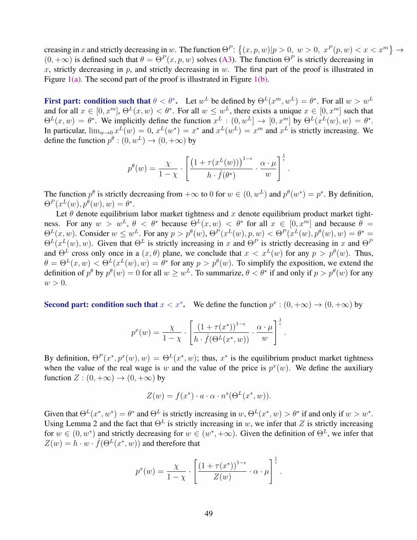
creasing in x and strictly decreasing inw. The function ΘP :{

(x, p, w)|p > 0, w > 0, xP (p, w) < x < xm}→

(0,+∞) is defined such that θ = ΘP (x, p, w) solves (A3). The function ΘP is strictly decreasing inx, strictly decreasing in p, and strictly decreasing in w. The first part of the proof is illustrated inFigure 1(a). The second part of the proof is illustrated in Figure 1(b).

First part: condition such that θ < θ∗. Let wL be defined by ΘL(xm, wL) = θ∗. For all w > wL

and for all x ∈ [0, xm], ΘL(x,w) < θ∗. For all w ≤ wL, there exists a unique x ∈ [0, xm] such thatΘL(x,w) = θ∗. We implicitly define the function xL : (0, wL] → [0, xm] by ΘL(xL(w), w) = θ∗.In particular, limw→0 x

L(w) = 0, xL(w∗) = x∗ and xL(wL) = xm and xL is strictly increasing. Wedefine the function pθ : (0, wL)→ (0,+∞) by

pθ(w) =χ

1− χ ·[(

1 + τ(xL(w)))1−ε

h · f(θ∗)· α · µw

] 1ε

.

The function pθ is strictly decreasing from +∞ to 0 for w ∈ (0, wL) and pθ(w∗) = p∗. By definition,ΘP (xL(w), pθ(w), w) = θ∗.

Let θ denote equilibrium labor market tightness and x denote equilibrium product market tight-ness. For any w > wL, θ < θ∗ because ΘL(x,w) < θ∗ for all x ∈ [0, xm] and because θ =ΘL(x,w). Consider w ≤ wL. For any p > pθ(w), ΘP (xL(w), p, w) < ΘP (xL(w), pθ(w), w) = θ∗ =ΘL(xL(w), w). Given that ΘL is strictly increasing in x and ΘP is strictly decreasing in x and ΘP

and ΘL cross only once in a (x, θ) plane, we conclude that x < xL(w) for any p > pθ(w). Thus,θ = ΘL(x,w) < ΘL(xL(w), w) = θ∗ for any p > pθ(w). To simplify the exposition, we extend thedefinition of pθ by pθ(w) = 0 for all w ≥ wL. To summarize, θ < θ∗ if and only if p > pθ(w) for anyw > 0.

Second part: condition such that x < x∗. We define the function px : (0,+∞)→ (0,+∞) by

px(w) =χ

1− χ ·[

(1 + τ(x∗))1−ε

h · f(ΘL(x∗, w))· α · µw

] 1ε

.

By definition, ΘP (x∗, px(w), w) = ΘL(x∗, w); thus, x∗ is the equilibrium product market tightnesswhen the value of the real wage is w and the value of the price is px(w). We define the auxiliaryfunction Z : (0,+∞)→ (0,+∞) by

Z(w) = f(x∗) · a · α · ns(ΘL(x∗, w)).

Given that ΘL(x∗, w∗) = θ∗ and ΘL is strictly increasing in w, ΘL(x∗, w) > θ∗ if and only if w > w∗.Using Lemma 2 and the fact that ΘL is strictly increasing in w, we infer that Z is strictly increasingfor w ∈ (0, w∗) and strictly decreasing for w ∈ (w∗,+∞). Given the definition of ΘL, we infer thatZ(w) = h · w · f(ΘL(x∗, w)) and therefore that

px(w) =χ

1− χ ·[

(1 + τ(x∗))1−ε

Z(w)· α · µ

] 1ε

.

49

0 0 xm

✓m

✓⇤

⇥L(x, wL)

⇥L(x, w < wL)xL(w)

⇥P (x, p✓(w), w)

⇥P (x, p > p✓(w), w)

✓

x

(a) Condition such that θ < θ∗

0 0 xm

✓m

✓⇤

✓

x x⇤

⇥P (x, px(w), w)

⇥P (x, p⇤, w⇤)

⇥L(x, w⇤)

⇥L(x, w > w⇤)

⇥P (x, p > px(w), w)

(b) Condition such that x < x∗

Figure A1: Illustration of the proof of Proposition 6

50

The properties of Z imply that the function px strictly decreasing for w ∈ (0, w∗) and strictly increas-ing for w ∈ (w∗,+∞) and px(w∗) = p∗.

Let θ denote equilibrium labor market tightness and x denote equilibrium product market tight-ness. Consider w ∈ (0,+∞). For any p > px(w), ΘP (x∗, p, w) < ΘP (x∗, px(w), w) = ΘL(x∗, w).Given that ΘL is strictly increasing in x and ΘP is strictly decreasing in x and ΘP and ΘL cross onlyonce in a (x, θ) plane, we conclude that x < x∗ for any p > px(w). To summarize, x < x∗ if and onlyif p > px(w) for any w > 0.

B Equilibrium ConceptThis appendix provides more details about our equilibrium concept. We draw a parallel betweenour concept and the Walrasian equilibrium. Following Walrasian theory, we make the institutionalassumption that a price, p, and a market tightness, x, are posted on the market for services, and wemake the behavioral assumption that buyers and sellers of services take price and tightness as given.The assumption is that buyers and sellers are small relative to the size of the market so that theyregard market tightness and price as unaffected by their own actions. Market tightness is the ratio ofaggregate buying effort to aggregate selling effort; thus, it seems reasonable for buyers and sellersto take it as given if they are small relative to the size of the market. The issue is more complicatedfor the price since buyer and seller could bargain over the price once they are matched, implying thatthey have some control over the price. However, the actual transaction price has no influence on theproduction and search decisions once a match is realized; what matters is the price that buyers andsellers expect to trade at. Since the transaction price depends on the other party and possibly otherfactors (for instance, custom, social norms, other buyers, and other sellers), we assume that each partytakes the expected transaction price as given.

We define a general equilibrium as follows:

DEFINITION A1. A general equilibrium is a price p, market tightness x, aggregate consumption ofservices c, aggregate sales of services s, a collection of visits {v(i), i ∈ [0, 1]}, and a collection ofcapacities {y(j), j ∈ [0, 1]} such that

(1) Taking x and p as given, buyer i ∈ [0, 1] chooses the number of visits v(i) to maximize her utilitysubject to her budget constraint and to the constraint imposed by matching frictions: c(i) =v(i) · q(x)/(1 + τ(x)), where c(i) is consumption of buyer i.

(2) Taking x and p as given, seller j ∈ [0, 1] chooses the capacity y(j) to maximize her utility subjectto the constraint imposed by matching frictions: s(j) = y(j) ·f(x), where s(j) is sales of seller j.

(3) The actual labor market tightness is x:

x =

∫ 1

0v(i)di∫ 1

0y(j)dj

.

(4) The price p is pairwise Pareto efficient in all buyer-seller matches.

(5) Aggregate consumption satisfies c =∫ 1

0c(i)di and aggregate sales satisfy s =

∫ 1

0s(j)dj.

51

As in a Walrasian equilibrium, our equilibrium concept imposes that buyers and sellers behaveoptimally given the quoted price and tightness. A key difference between the two equilibrium conceptsis that in a Walrasian equilibrium, buyers and sellers decide the quantity that they desire to buy or sellwhereas in our equilibrium, buyers and sellers decide the buying effort and selling effort that theydesire to exert, and these efforts lead to a trade with a probability determined by the market tightness.Consumers decide how many sellers of services to visit, knowing that each visits lead to a purchasewith probability q(x); workers decide how many units of services to offer for sale, knowing that eachunit is sold with probability f(x).

In a Walrasian equilibrium, the condition that sellers and buyers behave optimally is comple-mented by a market-clearing condition: at the quoted price, the quantity that buyers desire to buyequals the quantity that sellers desire to sell. It is possible to reformulate this condition as a consis-tency requirement: given that sellers and buyers expect to be able to trade with probability one, it mustbe that anybody desiring to trade is able to trade in equilibrium; this condition can only be fulfilledif the market clears. Condition (3) is the equivalent to this consistency requirement in presence ofmatching frictions. Once buyers and sellers have chosen {v(i), i ∈ [0, 1]} and {y(j), j ∈ [0, 1]}, thenumber of trades is given by[(∫

v(i)di

)−η+

(∫y(j)dj

)−η]−1η

=

(∫y(j)dj

)·f(∫

v(i)di∫y(j)dj

)=

(∫v(i)di

)·q(∫

v(i)di∫y(j)dj

).

These equalities imply that the selling probability faced by sellers is f(∫

v(i)di/∫y(j)dj

)and the

buying probability faced by buyers is q(∫

v(i)di/∫y(j)dj

). Both probabilities do not have to be

equal to the probabilities on which sellers and buyers based their calculations, f(x) and q(x). Inequilibrium, we impose the consistency requirement that these probabilities match, or equivalently,that the posted tightness equals the actual tightness,

∫v(i)di/

∫y(j)dj.

The last substantial equilibrium condition is that the price is pairwise Pareto efficient in all buyer-seller matches. In Walrasian theory, the condition that no mutually advantageous trades between twoagents are available impose that the probability to trade is one. This is because without a matchingfunction, buyers who do not trade with anybody but would like to trade can come together on themarket place. If excess supply or demand existed at the market price, buyers or sellers could initiatenew trades at a different price until all opportunities for pairwise improvement are exhausted. Forexample, if there is excess demand for a good, a buyer who is not receiving as much of the goodas she desires could offer a slightly higher price and get sellers to sell the good to her first, makingboth buyer and seller better off. In our theory, this condition only constrains the price to allocateto buyer and seller a positive share of the surplus arising from the seller-buyer match. This surplusarises because workers remain idle and do not sell one unit of service if the match is broken, and alsobecause buyer’s matching costs are sunk at the time of matching.

Under these equilibrium conditions, the market for nonproduced good necessarily clears:∫ 1

0m(i)di =

µ, where m(i) is consumption of nonproduced good by buyer i. The reason is that the budget con-straints of all consumers are satisfied, and that sales equal purchases through the matching process.

52

C Equilibrium Under Cobb-Douglas Utility FunctionWe determine conditions such that an equilibrium with positive consumption exists when consumershave Cobb-Douglas utility function (which is a CES utility function with ε→ 1). We state and provea proposition for the model of Section 2, and another one for the model of Section 3.

PROPOSITION A3. Consider the model of Section 2. Assume that consumers have a Cobb-Douglasutility function, cχ ·m1−χ. Define

pm ≡ χ

1− χ ·µ

y· (1− ρη)− 1

η .

There are two cases:

(i) If p ≤ pm, the only short-run equilibrium is (xm, 0).

(ii) If p > pm, one short-run equilibrium is (xm, 0) and one short-run equilibrium is (x, c) where xsatisfies

f(x) · y =χ

1− χ ·µ

p(A8)

and c = cs(x). In particular, x ∈ (0, xm) and c > 0.

Proof. We are looking for a tightness x ∈ [0, xm] that satisfies cs(x) = cd(x, p) or

1

1 + τ(x)·(f(x) · y − χ

1− χ ·µ

p

)= 0.

1/ (1 + τ(xm)) = 0 by definition of xm. Hence, (x, c) = (xm, cs(xm)) = (xm, 0) is always anequilibrium. Furthermore, 1/ (1 + τ(x)) > 0 for x < xm so any other equilibrium tightness mustsatisfy (A8). Since f is strictly increasing and f(0) = 0, there is a unique x ∈ (0, xm) that satisfiesthis condition if and only if

f(xm) = (1− ρη) 1η >

χ

1− χ ·µ

p · y . (A9)

Let us summarize the results. If (A9) is not satisfied, (xm, 0) is the unique equilibrium. If (A9) issatisfied, there are two equilibria: (xm, 0) and (x, c) where x satisfies (A8) and c = cs(x).

In the interior equilibrium (x, c), demand is higher than supply when tightness is below x (andconversely). Hence, if tightness is below equilibrium, demand is above supply, leading to an increasein tightness (and conversely). In contrast, in the corner equilibrium (xm, 0), demand is lower thansupply when tightness is below xm. Loosely speaking, the interior equilibrium is stable while thecorner equilibrium is unstable. Hence, the main text focuses solely on the interior equilibrium.

PROPOSITION A4. Consider the model of Section 3. Assume that consumers have a Cobb-Douglasutility function, cχ ·m1−χ. Define

Wm ≡ α · χ

1− χ · µ ·(1− ρη

) 1η .

53

Define Θ : [Wm,+∞) → [0, θm) by Θ(W ) = f−1 (α · [χ/ (1− χ)] · (µ/W )). Finally, define pm :[Wm,+∞)→ [0,+∞) by

pm(W ) =χ

1− χ ·µ

a· (1− ρη)− 1

η · [ns(Θ(W ))]−α .

There are two cases:

(i) If p · w ≤ Wm or p ≤ pm(p · w), there are two short-run general equilibria: the two equilibriawith zero consumption of Proposition A2.

(ii) If p ·w > Wm and p > pm(p ·w), there are three short-run general equilibria: the two equilibriawith zero consumption of Proposition A2 and (x, θ, n, c) where (θ, x) solve

α · χ

1− χ · µ = p · w · f(θ) (A10)

χ

1− χ · µ = p · f(x) · a · [ns(θ)]α (A11)

and n = ns(θ) and c = cs(x, n).

Proof. In general equilibrium, (x, θ) satisfies the system (A4)–(A5).

First case: θ = θm or x = xm. As explained in the proof of Proposition A2, there are exactly twogeneral equilibria in that case: the two equilibria with zero consumption of Proposition A2. Theseequilibria exist for any p > 0 and any w > 0.

Second case: θ < θm and x < xm. 1/(1 + τ(x)) > 0 and 1/(1 + τ(θ)) > 0 so we can rewrite (A4)and (A5) as

w · f(θ) = f(x) · a · α · [ns(θ)]α

f(x) · a · [ns(θ)]α =χ

1− χ ·µ

p.

The first equation is just (A2) and the second equation is just (A7) when ε = 1, substituting ns(θ) =h·f(θ)/(1+ τ(θ)). We can recombine this system as (A10)–(A11). The system (A10)–(A11) does not

admit solutions for any p and w. As we are looking for θ < θm, we need f(θ) < f(θm) =(1− ρη

) 1η .

Equation (A10) therefore requires

p · w > α · χ

1− χ · µ ·(1− ρη

)− 1η ≡ Wm.

Since f is strictly increasing from 0 to(1− ρη

) 1η for θ ∈ [0, θm), equation (A10) admits a unique

solution in [0, θm) if p · w > Wm. The function Θ defined in the proposition is the unique solutionto (A10) when p · w ∈ (Wm,+∞).

We turn to (A11). As we are looking for x < xm, we also need f(x) < f(xm) = (1− ρη) 1η .

54

Equation (A11) therefore requires

p >χ

1− χ ·µ

a· (1− ρη)− 1

η · [ns(Θ(p · w))]−α ≡ pm(p · w).

We replaced θ by Θ(p · w) in (A11) since we have already solved (A10) for θ. Since f is strictlyincreasing from 0 to (1− ρη) 1

η for x ∈ [0, xm), equation (A11) admits a unique solution in [0, xm) ifp > pm(p · w).

D Reducing Unemployment by Increasing WagesTo formalize the discussion of Section 3.6, we state and prove two propositions that apply to the modelwith customer relationships and inequality. The first proposition describes the set of parameters suchthat a general equilibrium exists. The second proposition establishes conditions such that a wageincrease leads to a reduction in unemployment.

PROPOSITION A5. Assume that consumers have Cobb-Douglas utility function, cχ ·m1−χ. Assumethat there are no matching costs: ρ = ρ = 0. Assume that the customer base is κ > 0. Normalizetechnology to a = 1 and price to p = 1. Then equilibrium employment solves

α

w· [K2 − κ] = K1 · n− κ · n1−α

where the constants K1 and K2 are defined by

K1 ≡∑

g(1− χg) · [α ·$g + (1− α) · σg]∑g(1− χg) · σg

(A12)

K2 ≡∑

g µg · χg∑g(1− χg) · σg

. (A13)

In addition, define the following constants: B1 ≡ κ−1/α ·(κ−K2)/(1−K1),B2 ≡ (κ−K2)/(κ−K1),andB3 ≡ (K1/K2)

1−αα . There are several possible cases in which a general equilibrium with positive

tightnesses exists:

(i) if K1 < κ, K2 < κ, and K1 < K2, for any wage such that (w/α) ∈ [B1, B2];

(ii) if K1 < 1, K2 < κ, and K1 > K2, for any wage such that (w/α) ∈ [B1, B3];

(iii) if K1 < 1, κ < K2, and K1 > K2, for any wage such that (w/α) ∈ [B2, B3];

(iv) if 1 < K1, κ < K2, and K1 > K2, for any wage such that (w/α) ∈ [B2,min {B1, B3}];In all these cases, the general equilibrium with positive tightnesses is unique.

Proof. Assume that ρ = ρ = 0, a = 1, and p = 1. In this case, τ(x) = τ(θ) = 0. Also assume thatκ > 0. A key general-equilibrium condition is that cd(n,w) = cs(x, n). Using the expressions forcs(x, n) and cd(n,w) obtained in Section 3.6, we obtain∑

g µg · χg∑g(1− χg) · σg

+

∑g χg · ($g − σg)∑g(1− χg) · σg

· w · n = κ · (1− f(x)) + f(x) · nα.

55

Another general equilibrium condition is that n = nd(θ, x, w), which implies α · f(x) = w · n1−α.Combining these two conditions, we obtain

α ·∑

g µg · χg∑g(1− χg) · σg

= α · κ− κ · w · n1−α +

[1− α ·

∑g χg · ($g − σg)∑g(1− χg) · σg

]· w · n.

Using the constants defined by (A12) and (A13), this equation simplifies to

α

w· (K2 − κ) = K1 · n− κ · n1−α. (A14)

Define the polynomial

P (z) = K1 · z1

1−α − κ · z +α

w· (κ−K2)

Solving the general equilibrium of the model is equivalent to solving P (z) = 0 and imposing that theroot z∗ of P satisfies z∗ ∈

[κ

1−αα ,min {1, α/w}

]. Once we have found z∗, the general equilibrium

(n, x, θ, c) is given by n = (z∗)1

1−α , x = f−1 (z∗ · w/α), θ = f−1(

(z∗)1

1−α

), and c = κ+(z∗ · w/α) ·(

(z∗)α

1−α − κ)

. The three conditions on z∗ ensure that we can construct x, θ, and c:

• z∗ ≥ κ1−αα ensures that c ≥ κ;

• z∗ < 1 ensures that we can construct θ given that f(θ) ∈ [0, 1];

• z∗ < α/w ensures that we can construct x given that f(x) ∈ [0, 1].

We first show that P (z) is strictly increasing for z ∈ [κ1−αα ,+∞).

P ′(z) =K1

1− α · zα

1−α − κ.

Hence,

P ′(κ1−αα ) =

[K1

1− α − 1

]· κ.

As

K1 =

∑g(1− χg) · [α ·$g + (1− α) · σg]∑

g(1− χg) · σg≥∑

g(1− χg) · [(1− α) · σg]∑g(1− χg) · σg

= 1− α,

K1/(1− α) ≥ 1 and P ′(κ1−αα ) ≥ 0. Since P ′ is strictly increasing for z ≥ 0, we infer that P ′(z) > 0

for z > κ1−αα . As a conclusion, P is strictly increasing for z ∈ [κ

1−αα ,+∞) and P has at most one

root on [κ1−αα ,+∞).

The system of equations has a solution if and only if P has a root in the interval[κ

1−αα ,min {1, α/w}

].

As a function of the parameters K1, K2, and κ, we determine for which wages such a root exists. Forsuch a root to exist, it is necessary and sufficient that P (κ

1−αα ) < 0 and min {P (1), P (α/w)} > 0.

The first condition is that P (κ1−αα ) < 0, which is equivalent to

w

α· (K1 − 1) < (K2 − κ) · κ− 1

α .

56

Define B1 ≡ κ−1/α · (κ−K2)/(1−K1). There are three cases:

• if K1 < 1, then we need w/α > B1;

• if K1 = 1, then any wage works as long as K2 > κ;

• if K1 > 1, then we need w/α < B1.

The next necessary condition is that P (1) > 0, which is equivalent to

w

α· (K1 − κ) > (K2 − κ).

Define B2 ≡ (κ−K2)/(κ−K1). There are three cases:

• if K1 < κ, then we need w/α < B2;

• if K1 = κ, then any wage works as long as K2 < κ;

• if K1 > κ, then we need w/α > B2.

The last necessary condition is that P (α/w) > 0, which is equivalent to

K1 ·(αw

) α1−α

> K2.

Define B3 ≡ (K1/K2)1−αα . Then we need w/α < B3 for any K1 > 0 and K2 > 0.

We now need to consider all the possible combinations of (K1, K2) to determine whether thereexists a wage satisfying these three conditions.

1. K2 < K1 < κ: We need w/α > B1, w/α < B2, and w/α < B3. K2 < K1 so B3 > 1 andB2 > 1. However, when w/α > 1, P (1) > P (α/w) so the constraint w/α < B2 is not binding.Hence, we only need to impose B1 < w/α < B3.

2. K1 < K2 < κ: We need w/α > B1, w/α < B2, and w/α < B3. K1 < K2 so B3 < 1 sow/α < 1 so P (1) < P (α/w) so the constraint w/α < B3 is not binding. Hence, we only needto impose B1 < w/α < B2.

3. K1 < κ and K2 > κ: We need w/α > B1, w/α < B2, and w/α < B3. But B2 < 0. Therefore,no such w/α exists.

4. K1 ∈ (κ, 1) and K2 < κ: We need w/α > B1, w/α > B2, and w/α < B3. But B2 < 0 so theconstraint w/α > B2 is always satisfied. Hence, we only need to impose B1 < w/α < B3.

5. K1 ∈ (κ, 1) and K2 ∈ (κ, 1) and K2 < K1: We need w/α > B1, w/α > B2, and w/α < B3.But B1 < 0 so the constraint w/α > B1 is always satisfied. Hence, we only need to imposeB2 < w/α < B3.

6. K1 ∈ (κ, 1) and K2 > K1: We need w/α > B1, w/α > B2, and w/α < B3. But B2 > 1 andB3 < 1. Therefore, no such w/α exists.

7. K1 > 1 and K2 < κ: We need w/α < B1, w/α > B2, and w/α < B3. But B1 < 0. Therefore,no such w/α exists.

57

8. K1 > 1 and K2 ∈ (κ,K1): We need w/α < B1, w/α > B2, and w/α < B3.

9. K1 > 1 and K2 > K1: We need w/α < B1, w/α > B2, and w/α < B3. But B2 > 1 andB3 < 1. Therefore, no such w/α exists.

Only Cases 1, 2, 4, 5, and 8 offer a solution.

PROPOSITION A6. In all general equilibria such thatK2 < κ, a wage increase leads to a reductionin unemployment, as well as an increase in employment, consumption, product market tightness, andlabor market tightness.

Proof. Consider a general equilibrium with K2 < κ. Using the notations of the proof of Proposition6, a general equilibrium characterized by z∗ satisfies P (z∗) = 0. We perform a comparative-staticsexercise with respect to w:

∂P

∂w+∂P

∂z· dz

∗

dw= 0.

Since K2 < κ,

∂P

∂w= α · (K2 − κ) · 1

w2< 0.

Furthermore, since z∗ > κ1−αα and K1 ≥ 1− α,

∂P

∂z=

K1

1− α · zα

1−α − κ ≥ zα

1−α − κ >(κ

1−αα

) α1−α − κ = 0.

We conclude that dz∗/dw > 0. All the results listed in the proposition follow given the relationshipbetween z∗ and the equilibrium variables described in the proof of Proposition 6.

58