1

A Modelling Study of the Multiphase Leakage Flow from Pressurised CO2

Pipeline

Xuejin Zhou a, Kang Li a, Ran Tu b, Jianxin Yi a, Qiyuan Xie a, Xi Jiang c * a Department of Safety Science Engineering & State Key Laboratory of Fire Science, University of Science and Technology of China, Hefei, Anhui 230026, China b College of Mechanical Engineering and Automation, Huaqiao University, Jimei, Xiamen, 361000, China c Engineering Department, Lancaster University, Lancaster LA1 4YR, United Kingdom

Abstract

The accidental leakage is one of the main risks during the pipeline transportation of high pressure CO2. The decompression process of high pressure CO2 involves complex phase transition and large variations of the pressure and temperature fields. A mathematical method based on the homogeneous equilibrium mixture assumption is presented for simulating the leakage flow through a nozzle in a pressurised CO2 pipeline. The decompression process is represented by two sub-models: the flow in the pipe is represented by the blowdown model, while the leakage flow through the nozzle is calculated with the capillary tube assumption. In the simulation, two kinds of real gas equations of state were employed in this model instead of the ideal gas equation of state. Moreover, results of the flow through the nozzle and measurement data obtained from laboratory experiments of pressurised CO2 pipeline leakage were compared for the purpose of validation. The thermodynamic processes of the fluid both in the pipeline and the nozzle were described and analysed.

Keywords: CO2; pipeline transport; choked flow; crack flow; equation of state

Nomenclature

Awall pipe inner surface area (m2)

Ae area of the leakage nozzle/orifice (m2)

c, c1, c2 sound speed (m/s)

cp,k heat capacity (J/Kg/K)

Cp,k extensive heat capacity (J/K/m3)

D the pipe inner diameter (m)

De diameter of the exit nozzle (m)

e specific internal energy (J/Kg)

* Corresponding author. Tel.: +44 1524 592439. E-mail address: x.jiang@lancaster.ac.uk.

2

E total energy of the fluid per unit volume (J/m3)

f the Fanning friction factor

h specific enthalpy (J/Kg)

H total enthalpy of the fluid per unit volume (J/m3)

M total mass of the fluid in the pipeline (Kg)

Ma Mach number

p pressure (Pa)

Q* CO2 mass outflow rates (Kg/s)

qwall heat flux at the pipeline wall (W/m2)

R universal gas constant (8.314 J/Kg/K)

s specific entropy of the fluid (J/Kg/K)

S entropy of the fluid (J/K)

T Temperature (K)

xg gas phase mass fraction

u fluid velocity (m/s)

v molar specific volume (m3/Kg)

V pipeline volume (m3)

ζk parameter in Eq. (7) (K/Pa)

ρ fluid density (Kg/m3)

Subscripts

0, 1, 2 parameters in the pipeline, nozzle inlet boundary, nozzle outlet boundary

g, d gaseous phase, liquid/dense phase

1. Introduction

The application of high pressure transmission pipelines to convey carbon dioxide in liquid/dense phase or supercritical phase is regarded as an essential element in the development of enhanced oil recovery and carbon capture and storage technologies. It is foreseen that large amounts of CO2 will be transported by pipelines if carbon capture and storage is deployed on an industrial scale [1]. Therefore it is important to ensure a safe and cost-effective implementation of the transportation.

Accidental release from pipelines could result in high concentrations due to the significant amounts of CO2 involved, leading to considerable negative impacts on the local environment and threats to the residents nearby [2]. Many pipeline failures caused by excessive stress, corrosion, and valve cracks are

3

initiated from small cracks or orifices [3, 4]. In order to detect and control the risks of these accidental failures in early stages, it is vital to understand and predict the leakage flow characteristics including the flow pressure and temperature, the exit velocity and the mass outflow rate [5]. Such data are important for the development of a leakage detection system and are critical when modelling the CO2 atmospheric dispersion because they provide the necessary input data and serve as the source terms for leakage strength estimation [6, 7].

Investigations of accidental release from high pressure hydrocarbon pipelines have long been a subject of study [8, 9]. The majority of the pipeline multiphase outflow numerical models in the literature is based on the homogeneous equilibrium mixture (HEM) [6, 10, 11] or more recently the homogeneous relaxation model (HRM) [12, 13]. The two models have been widely used and assessed by experimental data for hydrocarbon pipeline transport. For single-phase and two-phase flows, the choked flow condition in those studies is determined by maximizing the release mass flow rate with respect to the release pressure [14, 15], which may be more satisfied for full bore rupture of the pipeline in consideration of the almost instantaneous pressure drop at the rupture location. In the case of small puncture or orifice, the choked flow lasts much longer, while the pressure and temperature may vary violently in the cracks. Different from many other hydrocarbons, CO2 has a relatively high triple pressure of 0.518 MPa [16]. In addition to the Joule-Thomson effect, the temperature would experience a violent drop which means the cold condensed CO2 can be more likely appearing inside the cracks. It possesses high danger to pipeline integrity.

Numerical studies involving pressurised pipeline release through an orifice/nozzle have been conducted with different approaches. In some models [17, 18], the crack in the pipe wall is treated as a convergent nozzle and the choked flow condition was calculated elaborately for the nozzle. The calculations were mostly based on ideal gas and single phase flow, which are not suitable for applications of CO2 transport at typical operating conditions. Moreover, there are studies on the “rapid expansion of supercritical solution” solving the governing equations numerically, which calculate the choked flow from a stagnation source to the capillary exit [19, 20] explicitly. Overall, there is a lack of predictive models for high pressure leakage process taking into account both the flow in the pipe and the leakage flow through the nozzle with realistic equations of state. The thermo-hydraulic behaviour of accidental high pressure leakage flows has not been fully understood.

In this study, a one-dimensional fluid flow model was developed to investigate the leakage flow behaviour and the results were compared with the data obtained from an existing laboratory facility. The method is developed with two different equations of state for the multiphase mixture consideration. The main objective of the paper is to develop a simple but effective model for a better understanding of the thermo-hydraulic behaviour both in the pipeline and at the nozzle exit for the decompression process following the failure of pressurised CO2 pipelines.

2. Experimental setup

The experimental setup is shown in Fig. 1. The leakage experiments were performed in the laboratory facilities available at the University of Science and Technology of China [5, 21]. The high pressure CO2 circulation pipeline system is shown in Fig. 1(a). The test section is 10 m while the total length of the pipeline is 23 m. It consists of a carbon steel pipe with a 0.04 m outer diameter and 0.03 m inner diameter (1), which is designed with a maximum operating pressure of 16 MPa. The pipe is covered with a strip heater (2) and thermally insulated by a glass wool layer (3). The leakage module is settled in the middle of the pipe with a release nozzle (4) for controlling the initiation of the leakage.

4

The cross-sectional view of this leakage module is shown in Fig. 1(b). At the beginning, CO2 was pressurised and cooled down to liquid phase; then it would be injected into the pipe, and be heated or pressurised continuously by a pump to maintain a specific equilibrium pressure, temperature and phase conditions. At last, the CO2 was released through the leakage module. In this process, the pressures of the fluid and the temperatures of the wall were measured with pressure transducers and thermal couples which were distributed along the test pipe as schematically shown in Fig. 1(a).

Three experiments with different initial conditions were performed using a release nozzle diameter of 2.5 mm with a length of 150 mm, which were summarised in Table 1. These experiments were designed with different initial conditions which include supercritical, near-critical and gas-like phases. The results will be presented and used to validate the predictions using the mathematical model developed in this study.

The uncertainty in the pressure measurements in the pipeline and nozzle is ±0.25%, while the uncertainty in the temperature measurements is ±5%. The mass inside the pipeline is calculated using the measured pressure and temperature. The flow rate is the time derivative of the mass of CO2 inside the pipeline with an uncertainty of ±21%. These are based on systematic assessments of the experimental procedures and measurement data.

Fig. 1 (a) Overview of the test section. (b) The cross-sectional view of the leakage module.

Table 1. Operating conditions and initial parameters in the experiments.

Properties Test 1 Test 2 Test 3

Initial Pressure (MPa) 8.94 7.97 6.96

Temperature (◦C) 40.0 40.0 39.8

Phase state Supercritical Supercritical Gas

3. Modelling approach

3.1 Thermodynamic properties

A pivotal prerequisite condition for the computational study involving pressurised CO2 is to calculate its thermodynamic properties accurately over a wide range of pressure and temperature. In

5

the case of CO2 release from high pressure reservoirs, it has been shown that the temperature could drop to the triple point [16, 21], resulting to high density substance including “dry ice”. The PT phase diagram of CO2 [22] is shown in Fig. 2. Since the high pressure CO2 release involves significant phase changes, any equation of state employed must be consistent with the real gas behaviours covering a range of conditions including the critical point and the triple point.

To satisfy the requirements, two kinds of equations of state are used in this study: Span-Wagner equation of state (SW EOS) and Peng-Robinson equation of state (PR EOS). The SW EOS [23] which explicitly employs the Helmholtz free energy has a complex format for the state of CO2. It is considered as the most accurate and the state-of-the-art equation of state for CO2, which can be used to benchmark simpler equations for gas and liquid phase densities. The PR EOS [24] extends the ideal gas state equation to a cubic equation using a simple format. It can be written in a common format:

( ) ( )RT ap

v b v v b b v b= −

− + − − (1)

where the coefficients a and b are defined elsewhere [24].

Fig. 2 Schematic of the phase diagram for carbon dioxide, data from [22].

Fig. 3 presents the ρ-T saturation curve obtained using the PR EOS in comparison with SW EOS. It shows that PR EOS is close to SW EOS in the gas phase, but the liquid densities given by the two equations do not agree well. It means PR EOS may result in large uncertainty in the liquid phase calculation. Fig. 3 also shows CO2 density variations corresponding to three pressures and the experimental initial conditions (green cross markers). In this study, Chung’s method is used to obtain the viscosity [25] during the decompression process. All the calculations performed are based on these equations.

6

Fig. 3 Density on the saturation curve obtained using the PR EOS and SW EOS, and density variations with three pressures (thin solid lines).

3.2 Homogenous equilibrium model

The present study is dedicated to modelling the choked flow characteristics with homogeneous equilibrium assumption. In this study, the mixture of CO2 is considered to be in dense form (including supercritical fluid, liquid phase) and gaseous form. The HEM is based on assumptions of thermal and dynamic equilibrium between the phases, which means they move in the same velocity and have the same temperature. In addition, the mixture pressure is assumed to be equal to the saturated pressure whenever the liquid and gas coexist.

Properties of the HEM fluid are essential to the computational model of CO2 release process. The specific molar volume v, specific enthalpy h, and specific entropy s are defined as:

(1 )g g g dv x v x v= + − (2)

(1 )g g g dh x h x h= + − (3)

(1 )g g g ds x s x s= + − (4)

where the subscript g denotes the gaseous phase, d the dense/liquid phase. The fluid properties of single phase are calculated with the two equations of state.

3.3 Speed of sound

When a CO2 dense/liquid–gas mixture remains in equilibrium, the adiabatic sound speed of a pure component is given by:

1/2

S

pcρ

∂= ∂

(5)

When the pressure is in equilibrium, we can differentiate Eq. (2) with respect to p,

7

22 2 2 2 21

11 = g g

g g d d

x xc c c

ρρ ρ

−+

(6)

where cg and cd are adiabatic sound speed of dense/liquid and gas phases respectively, while c1 is the mixture sound speed assuming pressure equilibrium.

When both pressure and temperature are in equilibrium, the mixture sound speed is given by [26]:

( )2

, ,2 22 1 , ,

1 1 p g p d d g

p g p d

C Cc c T C C

ζ ζρ −= +

+ (7)

where for { , }k g d∈ , variable kζ and ,p kC are defined as:

k

ks

Tp

ζ ∂

= ∂ (8)

, ,p k k k p kC x cρ= (9)

,k

p kp

c T sT∂∂

=

(10)

In this paper, c2 is used to represent the mixture sound speed. The mixture sound speed for CO2 at the boiling point T = 273.15 K is presented in Fig. 4. The data show that the results from the two equations differ from each other considerably.

Fig. 4 Mixture sound speed of two-phase CO2 as a function of gas mass fraction.

8

3.4 Computational model

When modelling the leakage flow of CO2 from a pressurised pipeline, either the adiabatic flow model (the Fanno flow) [27], assuming no external heat transfer, or the isothermal flow model, assuming that the heat flux received cross the pipe wall leads to a constant temperature, can be used. Both of them could apply to a one-dimensional, transient compressible model based on the HEM assumption. The continuity, momentum, and energy conservation equations in a pipeline are respectively given by

( ) 0ρ ρut x

∂ ∂+ =

∂ ∂ (11)

2 2( ) ( ) 2ρu ρu p fρut x x D

∂ ∂ ∂+ + = −

∂ ∂ ∂ (12)

34[( ) ] 2wallqE E p u fρut x D D

∂ ∂ ++ = − −

∂ ∂ (13)

where f can be calculated by Colebrook equation [28]. E is the total energy of the fluid per unit volume:

2( 2)E e uρ= + (14)

where e = h – p/ρ can be associated with a single-phase or a multi-phase flow. Since the pipe is well insulated, the heats transfer between the pipe and surrounding materials can be ignored. Furthermore, if the total heat capacity is relatively small, the pipe decompression is simulated as an adiabatic process without any heat source terms.

The schematic of the overall leakage model is shown in Fig. 5. Three specific states of the flow named J0, J1, J2 represent the average state of the pipe flow, the flow at the nozzle inlet boundary and flow at the nozzle outlet boundary, respectively. Therefore, the leakage process is divided into two parts: from the pipe to nozzle inlet (J0 to J1) and inside the nozzle (J1 to J2). They are solved with the vessel blowdown model and capillary tube assumption respectively and coupled with each other in J1. Both calculations are derived from the above equations with different simplifications. The following section will give a detailed description.

9

Fig. 5 Schematic representations of the CO2 pipe flow and nozzle flow analyses.

3.4.1 Vessel blowdown model

For short pipelines or reservoirs with small orifices/nozzles, the blowdown model can be used to simulate the decompression process [15]. It can be considered as a zero-dimensional pipeline release model where the momentum of the fluid upstream the release unit is neglected [29]. Inside the pipeline, the HEM is employed in which assumptions of local thermodynamic equilibrium and isentropic flow are adopted. The density is calculated by a mass balance and an energy balance:

0ddd dM V Qt t

ρ ∗= = − (15)

0 01

d( )d waal ll lw

Mh p V Q h q At

∗−= − + (16)

where ρ0, p0 and h0 are the average properties in the pipeline J0; h1 is the instantaneous specific enthalpy of the leakage flow. The heat transfer rate is defined as qwallAwall. Due to the slow cooling of the pipe wall, the heat transfer should not be neglected here as the leakage process lasted for a long time (hundreds of seconds) for the small nozzle. It is shown that the decompression process is highly turbulent and characterised by intense heat transfer from the pipe wall to the colder fluid [5, 11]. So it is reasonable to assume that the thermal boundary layer at the pipeline wall is infinitely thin, hence the heat flux is applied directly to the fluid. In this research, the pipe wall temperature is measured by thermocouples, and qwall is obtained from a calculation of the heat flux.

Using the thermodynamic relation of dh = Tds + vdp, Eq. (10) can be expressed as:

*00 0 0 1

d ( )dsVT Q h ht

ρ = − (17)

10

3.4.2. The choked flow calculation In this study, the pipeline leaks at time t = 0, and the choked flow is formulated in the release point

momentarily. Accordingly, the variables need to be solved are the choked flow parameters: Q* and h1, which will be described in this section.

As mentioned above, parameters in J0 are determined by the blowdown model. However, the exit nozzle inlet boundary J1 cannot take the values in J0 when the flow is choked since the local flow field will be significantly different from the average ones. Instead, J0 and J1 share the same specific entropy only since the decompression process in the pipeline is considered to be isentropic. Generally, the two sub-models are solved separately but linked by the mass outflow rate, entropy and enthalpy in the nozzle.

With respect to the crack geometry structure, the main challenge is to evaluate the choked flow parameters in the leakage module. The flow going through the nozzle to the exit J2 is assumed to be fast and therefore an adiabatic and quasi-steady state assumption could be used. Moreover, the cross-sectional area of the nozzle does not decrease consistently, so that a convergent nozzle assumption cannot be employed to deal with the area change. In the present study, the capillary tube assumption for the leakage module is superseded which has been used similarly in the rapid expansion of supercritical solution [20]. For the capillary process, the typical analysis involves the quasi-one-dimensional approximation including viscous frictional effects. A strong gradient of pressure and temperature exists in the tube flow to overcome the viscous wall shear and accelerate the fluid from stagnation condition to sonic conditions at the exit. Unlike the convergent nozzle model in which the area change dominates the acceleration, the capillary flow is not isentropic. In this model, the heat transfer in the capillary tube is neglected and the flow is considered as adiabatic and in quasi-steady state, so that the governing equations Eqs (11) - (13) can also be used here. Fanno equations of conservation of mass, momentum and energy are respectively expressed as:

*

e

QuA

ρ = (18)

2d d 2d d e

p u fuux x D

ρ+ = − (19)

( )2d 20

dh u

ρux

+= (20)

Here the length of the capillary tube is set as the length from the valve to the nozzle outlet. The energy conservation equation can be expressed by the total enthalpy per unit volume 2( 2)H h u= + , which is a constant in the nozzle.

The capillary tube inlet boundary conditions are imposed by the pipeline conditions: the specific entropy s1 in J1 is specified to be equal to s0 in J0. While at the outlet, the boundary conditions depend on the pressure ratio between p2 and p1, as that shown in the bottom right sub-figure of Fig. 5. When the ratio is subcritical, the leakage flow is not choked therefore parameters in J0 are applied to J1 and the atmospheric pressure is imposed at the outlet boundary. Otherwise when the pressure ratio is supercritical or critical (the “critical” here is an aerodynamic concept of sonic flow instead of the CO2

11

thermodynamic state), the flow is choked, and the flow accelerates to a sonic condition which means the Mach number at the exit J2 is equal to one:

22

2

1uMac

= = (21)

Eqs. (18) – (21) can be solved numerically with an auxiliary equation of state and initial condition. The Q* and the h1 here are incorporated with Eqs. (15) and (17) to accomplish the vessel blowdown model.

Fig. 6 Numerical algorithm for solving the vessel blowdown model equations (left diagram); iterative procedures to complete the choked flow calculation (right diagram).

3.4.3. Numerical algorithm The numerical algorithm for solving the equations is shown by the flowcharts in Fig. 6. When

started, J0 is given for the choked flow calculations which involve iterative procedures by Eqs. (18) -(21), shown in the right-hand side of the figure. Then Q*and h1 are updated and returned to the vessel blowdown model. This algorithm involves explicit time integration of Eqs. (15) and (17).

4. Results and discussion

In this section, the results of Tests 1-3 are analysed and used to validate the proposed computational model. Furthermore, a brief discussion on the multiphase flow characteristics by investigating the vapour mass fraction and exit conditions is also presented.

4.1 Decompression process

The experimental data of three tests in Table 1 indicate that the pressure measured along the pipe had small variations for all the tests (not presented for brevity) during the decompression process, so that the vessel blowdown model is suitable to simulate the above tests. In Figs. 7 and 8, both the

12

experimental results and the corresponding simulation results including the pipeline pressure and the mass flow rate calculated as functions of time are presented. Additionally, in Test 1 and Test 2 the fluid was initially in supercritical state, but in Test 2 it was closer to the critical point. The initial phase condition in Test 3 was gas-like.

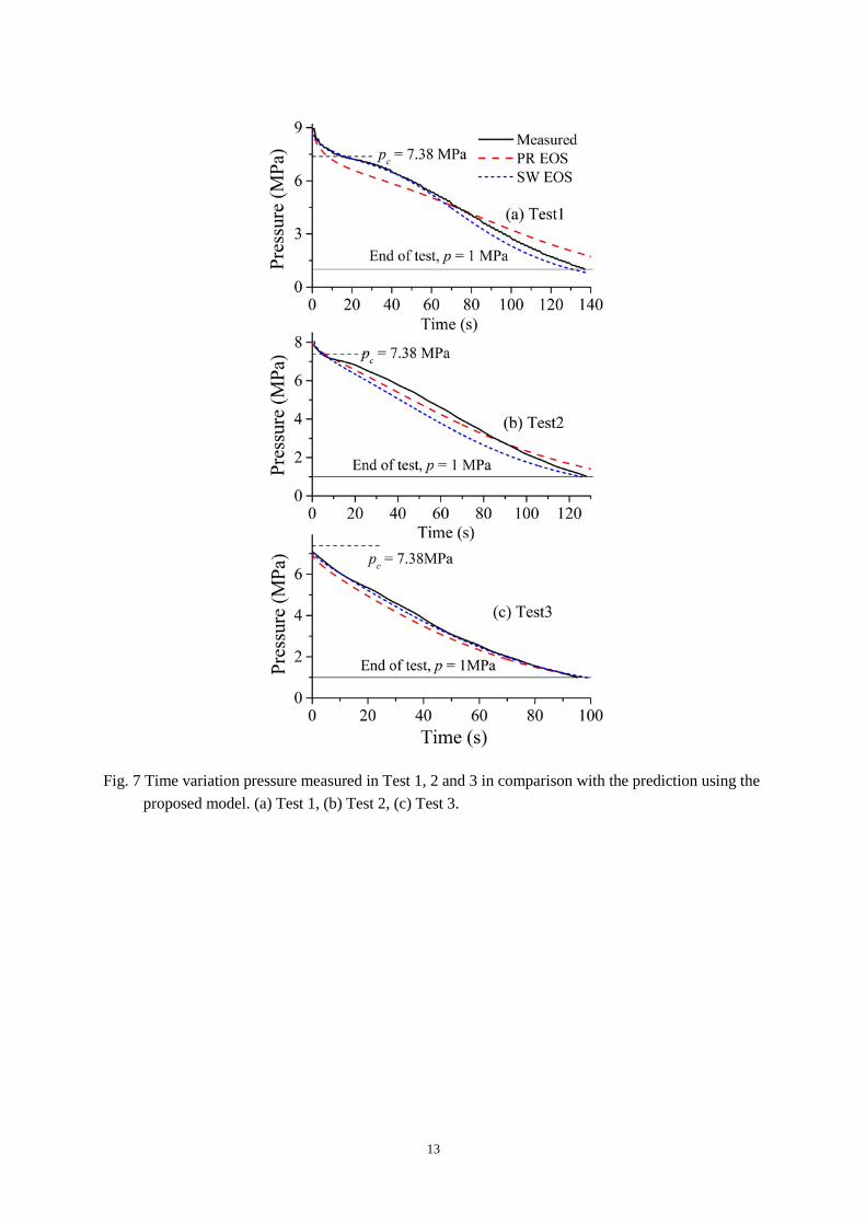
Figs. 7(a) - (c) present the pipeline pressure transients measured in Tests 1, 2 and 3 in comparison with the prediction using the coupled model employing PR EOS and SW EOS, respectively. As can be seen, the pressure decreases nearly linearly on the whole with time from the initial decompression. All the three predictions are in good agreements with the experimental data. One main significant difference can be seen from Figs. 7(a) - (b) is that the pressures in Tests 1-2 (black line) experience an obvious sudden drop in the very early stage (before t = 14 s in Test 1 and t = 7 s in Test 2). This phenomenon is caused by phase-state changes between the pure supercritical and the gas phases or two-phase mixtures. More discussions on this will be provided in the next section. The subsequent linear but slower decreases are observed and in agreement with previous saturated fluids decompression studies reported [29, 30].

When comparing the predictions of Test 1 (dashed lines) to the measured data, the model could catch the pressure drop tendency in the early stage. The predicted value agreed with the measurements and the decreasing trend quite well. However, when using PR EOS in the modelling approach, the pressures were considerably under-predicted in that period and the time when the quick drop ceased was not satisfactorily predicted. The reason may be that the equation of state greatly differs from the real gas near the critical point, as can be seen in Fig. 3. In addition, the difference between them tends to decrease when the initial condition was gaseous, as shown in Fig. 7(c). The pressure transients shown in Fig. 7(a) are well represented by the model with SW EOS in the first 60 s. The predictions are somewhat lower afterwards. Similarly, such discrepancies, although to a less extent, are also observed in Figs. 7(b)-(c). One reason for this could be the inaccurate prediction of heat transfer to the wall. Another possible reason for the discrepancies may be that the fluid was an unsaturated mixture of liquid–gas from J0 to J2, and thus cannot be accurately modelled by the HEM assumption.

13

Fig. 7 Time variation pressure measured in Test 1, 2 and 3 in comparison with the prediction using the proposed model. (a) Test 1, (b) Test 2, (c) Test 3.

14

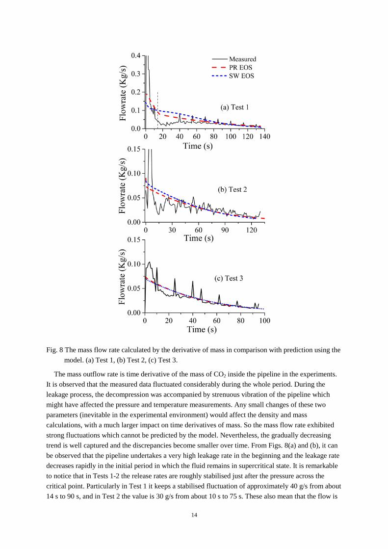
Fig. 8 The mass flow rate calculated by the derivative of mass in comparison with prediction using the model. (a) Test 1, (b) Test 2, (c) Test 3.

The mass outflow rate is time derivative of the mass of CO2 inside the pipeline in the experiments. It is observed that the measured data fluctuated considerably during the whole period. During the leakage process, the decompression was accompanied by strenuous vibration of the pipeline which might have affected the pressure and temperature measurements. Any small changes of these two parameters (inevitable in the experimental environment) would affect the density and mass calculations, with a much larger impact on time derivatives of mass. So the mass flow rate exhibited strong fluctuations which cannot be predicted by the model. Nevertheless, the gradually decreasing trend is well captured and the discrepancies become smaller over time. From Figs. 8(a) and (b), it can be observed that the pipeline undertakes a very high leakage rate in the beginning and the leakage rate decreases rapidly in the initial period in which the fluid remains in supercritical state. It is remarkable to notice that in Tests 1-2 the release rates are roughly stabilised just after the pressure across the critical point. Particularly in Test 1 it keeps a stabilised fluctuation of approximately 40 g/s from about 14 s to 90 s, and in Test 2 the value is 30 g/s from about 10 s to 75 s. These also mean that the flow is

15

highly choked. After that, the leakage rates keep slowing down until the end of test.

The model with either equation of state could reproduce the general trends of the experimental data, especially the slower decreasing periods. When the initial condition is in a gas-like state (Fig. 7(c)), the mass flow rates predicted are in very close agreement with the experimental data. However, the predictions and experimental data do not match well in the early stages of the leakage, with the predicted values obviously changing slower compared with the tests. The large deviation at the beginning can be mainly attributed to the simplified calculation of the chocked flow. For the experimental tests, the pressure at the outlet boundary (p2) was equal to the local atmospheric pressure at the start which increased sharply after the test began. While the model calculation for the pressure (indicated by the algorithm shown in Fig. 6) neglected the transient period. Accordingly p2 in the model is much larger than the real pressure at the beginning, so is the pressure ratio (p2/p1). Therefore, large deviations occurred as shown in Figs. 8(a) and (b). Moreover, an observation in Figs. 8(a) and (b) is that the flow remained roughly at a constant release rate after the appearance of the two-phase mixture, while the model predicted a decreasing trend. At the start of the release test, the mass outflow quickly attained its maximum level with the initial high pressure inside the pipeline. The fluid through the nozzle experienced a violent drop in both pressure and temperature which led to considerable phase changing to saturation. This leakage flow soon became choked and the outflow rate decreased from the maximum level. As the inner pressure is maintained, the mass flow rate reaches a quasi-steady state. After transition from saturation to gaseous flow the mass flow rate dropped further. Since the multiphase behaviour of the flow was not captured in the model, the simplification in the choked flow calculation led to the discrepancies between the modelling and experimental results. Although the proposed model captures the main flow features of the decompression process, there are still large rooms for further improvements.

4.2 Test analyses

The variations of gas mass fraction with time, predicted using the flow models both inside the pipeline and at the nozzle outlet J2 for Test 1, are shown Fig. 9. Although the only difference is 1 MPa in the initial pressure, Test 2 does not experience a two-phase period in the pipeline. For brevity, only Test 1 is shown here as a typical case. In the case of an adiabatic release, the fluid could remain two-phase over the entire period of release once the condition is met [15]. In this study, since the heat transfer to the wall was taken into account, the two-phase state only lasted for a few seconds. It means that the heat transfer can promote the liquid vaporisation.

16

Fig. 9 Gas mass fraction predicted in J0 and J2 for Test 1.

Given that the pipeline flow is supercritical initially, the gas fraction remains zero at first, which refers to a rapid decrease of pressure and temperature. Then the supercritical fluid turns into a saturated mixture. The models with either PR EOS or SW EOS captured this characteristic satisfactorily. During the vaporisation process, gas mass fraction calculated with PR EOS was obviously lower than that with SW EOS. The vaporisation completed at ca. 23 s for SW EOS and 75 s for PR EOS, respectively. It is mainly due to the under-prediction of pressure in PR EOS, as shown in Fig. 7(a). Interestingly, situation in the nozzle exit J2 is quite different from the pipeline J0. The exit velocity of the flow, shown in Fig. 11, is accelerated to sonic from J0 to J2. The inner energy, pressure and temperature of the fluid would undertake a sharp drop, leading to a longer duration of two-phase flow from the very beginning in J2.

In Fig. 10, the modelling results are plotted in PT-diagrams together with the boiling line of pure CO2. It gives a visual comparison of the decompression process in the nozzle inlet J0 and nozzle outlet boundary J2. The results also show that the supercritical fluid changes to liquid-gas phase in J2 from the beginning. Furthermore, it implies that the pressure and temperature are much lower in the nozzle.

Uncontrolled depressurization of liquid or dense phase CO2 can lead to temperatures below the design temperature of the pipeline, as well as the high speeds. It is reasonable to believe that cold condense CO2 passing through the cracks could lead to catastrophic damage to the pipeline. A fully understanding of the pipeline decompression in the pipe wall is important for the long-term emergency planning in the case of accidental failure of long CO2 transportation pipelines. The model presented above may be used to access the risks. The model predictions can also provide source terms for CO2 vapour dispersion modelling, which can assist the leakage detection technology development.

17

Fig. 10 p-T variations in J0 and J2 for Test 1 plotted together with the boiling line.

Fig. 11 Nozzle exit velocity predicted for Test 1.

5. Conclusion remarks

This work studied the decompression of a high pressure CO2 transportation pipe. Using two sub-models for the two-stage leakage process, a modelling approach was developed to evaluate the leakage flow through a nozzle in the pipe. As the model formulation is relatively simple and easy to implement, the modelling approach can be advantageous in practical engineering applications. The pipeline decompression model based on the blowdown model was further incorporated with the capillary tube assumption for calculating the choked flow condition. Two kinds of equations of state were employed to take the two-phase flow into account. Comparisons with experimental data were performed. According to the results, some conclusions are summarised as follows:

(1) Comparison of the model predictions with the experimental data showed that the model accurately predicts the pressure variation tendencies in the pipe in the three tests. In the case of initially supercritical CO2 fluid (Tests 1 and 2) the disagreements can be attributed to the equation of state and the HEM assumption.

(2) Generally, the more complex and accurate SW EOS shows a better prediction than the PR EOS. The PR EOS may compromise the accuracy in dealing with the flow which involves significant phase changes, especially near the critical point. Since it is much simpler with low computational costs, the PR EOS may be effectively used in the case of single phase flows or liquid-gas flows.

(3) The proposed model also accounts for the effects of heating in the pipe and viscous friction at the nozzle. The non-adiabatic decompression process varies significantly near the critical point.

18

(4) The flow is choked when initiated from supercritical phase, and stabilised release rates are observed after the critical point.

(5) Remarkable temperature drop and velocity increase in the crack can be potentially dangerous to the pipeline integrity.

The choked flow calculation depends on the pressure and temperature at the inlet boundary near the leakage nozzle, the equations of state and other assumptions used. To improve the modelling capability, the model can be subsequently extended to three-phase flow simulation in a straightforward manner. Further studies will be aimed at taking into account the solid phase and vapour dispersion in the physical modelling as well as the vibration behaviour of the pipe during the leakage.

Acknowledgements

This work was supported by the Thousand Talent Programme of China, China Postdoctoral Foundation (Project No. 2012M521253), National Natural Science Foundation of China (No.51106147) and National Basic Research Programme of China (973 Programme: No. 2012CB719701). The authors thankfully acknowledge all these supports.

19

References [1] B. Metz, O. Davidson, H. de Coninck, M. Loos, L. Meyer. IPCC special report on carbon dioxide

capture and storage. Cambridge University Press, UK 2005; p. 181-85. [2] J. Koornneef, M. Spruijt, M. Molag, A. Ramírez, W. Turkenburg, A. Faaij. Quantitative risk

assessment of CO2 transport by pipelines—A review of uncertainties and their impacts. J Hazard Mater. 177(1–3) (2010) 12-27.

[3] M.T. Lilly, S.C. Ihekwoaba, S.O.T. Ogaji, S.D. Probert. Prolonging the lives of buried crude-oil and natural-gas pipelines by cathodic protection. Appl Energ. 84(9) (2007) 958-70.

[4] S. Rimkevicius, A. Kaliatka, M. Valincius, G. Dundulis, R. Janulionis, A. Grybenas, I. Zutautaite. Development of approach for reliability assessment of pipeline network systems. Appl Energ. 94 (2012) 22-33.

[5] K. Li, X. Zhou, R. Tu, Q. Xie, X. Jiang. The flow and heat transfer characteristics of supercritical CO2 leakage from a pipeline. Energy. 71 (2014) 665-72.

[6] A. Oke, H. Mahgerefteh, I. Economou, Y. Rykov. A transient outflow model for pipeline puncture. Chem Eng Sci. 58(20) (2003) 4591-604.

[7] E. Papanikolaou, M. Heitsch, D. Baraldi. Validation of a numerical code for the simulation of a short-term CO2 release in an open environment: Effect of wind conditions and obstacles. J Hazard Mater. 190(1–3) (2011) 268-75.

[8] A. Luketa-Hanlin. A review of large-scale LNG spills: Experiments and modeling. J Hazard Mater. 132(2–3) (2006) 119-40.

[9] Z.Y. Han, W.G. Weng. Comparison study on qualitative and quantitative risk assessment methods for urban natural gas pipeline network. J Hazard Mater. 189(1–2) (2011) 509-18.

[10] M. Popescu. Modeling of fluid dynamics interacting with ductile fraction propagation in high pressure pipeline. Acta Mech Sin. 25(3) (2009) 311-18.

[11] S. Martynov, S. Brown, H. Mahgerefteh, V. Sundara. Modelling choked flow for CO2 from the dense phase to below the triple point. Int J Greenh Gas Con. 19 (2013) 552-58.

[12] K. Banasiak, A. Hafner. Mathematical modelling of supersonic two-phase R744 flows through converging–diverging nozzles: The effects of phase transition models. Appl Therm Eng. 51(1–2) (2013) 635-43.

[13] S. Brown, S. Martynov, H. Mahgerefteh, C. Proust. A homogeneous relaxation flow model for the full bore rupture of dense phase CO2 pipelines. Int J Greenh Gas Con. 17 (2013) 349-56.

[14] E. Elias, G.S. Lellouche. Two-phase critical flow. Int J Multiphas Flow. 20, Supplement 1 (1994) 91-168.

[15] S. Martynov, S. Brown, H. Mahgerefteh, V. Sundara, S. Chen, Y. Zhang. Modelling three-phase releases of carbon dioxide from high-pressure pipelines. Process Saf Environ. PSEP-379. (2013).

[16] A. Mazzoldi, T. Hill, J.J. Colls. CO2 transportation for carbon capture and storage: Sublimation of carbon dioxide from a dry ice bank. Int J Greenh Gas Con. 2(2) (2008) 210-18.

[17] A. Morin, S. Kragset, S.T. Munkejord. Pipeline flow modelling with source terms due to leakage: the straw method. Energy Procedia. 23 (2012) 226-35.

[18] H.O. Nordhagen, S. Kragset, T. Berstad, A. Morin, C. Dørum, S.T. Munkejord. A new coupled fluid–structure modeling methodology for running ductile fracture. Comput Struct. 94–95 (2012) 13-21.

[19] I.G. Khalil, D.R. Miller. The structure of supercritical fluid free-jet expansions. Aiche J. 50(11) (2004) 2697-704.

[20] I.G. Khalil, D.R. Miller. The free-jet expansion of supercritical CO2 from a capillary source. AIP Conference Proceedings. 762(1) (2005) 343-48.

[21] Q. Xie, R. Tu, X. Jiang, K. Li, X. Zhou. The leakage behavior of supercritical CO2 flow in an experimental pipeline system. Appl Energ. 130 (2014) 574-80.

[22] E. Lemmon, M. McLinden, D. Friend, P. Linstrom, W. Mallard. NIST chemistry WebBook, Nist standard reference database number 69. Thermophysical Properties of Fluid Systems, National Institute of Standards and Technology, Gaithersburg. 2010.

20

[23] R. Span, W. Wagner. A new equation of state for carbon dioxide covering the fluid region from the triple ‐point temperature to 1100 K at pressures up to 800 MPa. J Phys Chem Ref Data. 25(6) (1996) 1509-96.

[24] D.Y. Peng, D.B. Robinson. A new two-constant equation of state. Industrial & Engineering Chemistry Fundamentals. 15(1) (1976) 59-64.

[25] T.H. Chung, M. Ajlan, L.L. Lee, K.E. Starling. Generalized multiparameter correlation for nonpolar and polar fluid transport properties. Industrial & Engineering Chemistry Research. 27(4) (1988) 671-79.

[26] T. Flatten, H. Lund. Relaxation two-phase flow models and the subcharacteristic condition. Mathematical Models and Methods in Applied Sciences. 21(12) (2011) 2379-407.

[27] P.K. Bansal, G. Wang. Numerical analysis of choked refrigerant flow in adiabatic capillary tubes. Appl Therm Eng. 24(5–6) (2004) 851-63.

[28] B.R. Munson, W.W. Huebsch, A.P. Rothmayer. Fundamentals of fluid mechanics. New York: John Wiley & Sons, Inc., 1998.

[29] A. Fredenhagen, R. Eggers. High pressure release of binary mixtures of CO2 and N2. Experimental investigation and simulation. Chem Eng Sci. 56(16) (2001) 4879-85.

[30] S.M. Richardson, G. Saville, S.A. Fisher, A.J. Meredith, M.J. Dix. Experimental Determination of Two-Phase Flow Rates of Hydrocarbons Through Restrictions. Process Saf Environ. 84(1) (2006) 40-53.