Under consideration for publication in Math. Struct. in Comp. Science

A Modular Formal Semantics for Ptolemy1 2

Stavros Tripakis, Christos Stergiou, Chris Shaver and Edward A. Lee

University of California, Berkeley

{stavros,chster,shaver,eal}@eecs.berkeley.edu

Received 23 August 2012

Ptolemy is an open-source and extensible modeling and simulation framework. It offersheterogeneous modeling capabilities by allowing different models of computation, both untimedand timed, to be composed hierarchically in an arbitrary fashion. This paper proposes a formalsemantics for Ptolemy which is modular, in the sense that atomic actors and their compositions aretreated in a unified way. In particular, all actors conform to an executable interface that containsfour functions: fire (produce outputs given current state and inputs), postfire (update stateinstantaneously), deadline (how much time the actor is willing to let elapse) and time-update(update state with passage of time). Composite actors are obtained from composition operators thatin Ptolemy are called directors. Different directors realize different models of computation. Thispaper defines formally the directors for the following models of computation:Synchronous-Reactive, Discrete Event, Continuous Time, Process Networks, and Modal Models.

Contents

1 Introduction 22 Related Work 63 Ptolemy’s Graphical Syntax 114 Actors 13

4.1 Variables, Assignments and Timers 134.2 Actors 134.3 Actor Behaviors 144.4 Actor Classification and Special Cases 154.5 Examples of Atomic Actors 15

1 Ptolemy in this document refers to Ptolemy II, see http://ptolemy.org. If you are reading this document onscreen (vs. on paper) and you have a network connection, then you can click on the figures showing Ptolemy models toview, execute and experiment with those models online. There is no need to pre-install Ptolemy or any other software.

2 This work is partially supported by NSF project ExCAPE: Expeditions in Computer Augmented Program Engineering,and by the Center for Hybrid and Embedded Software Systems (CHESS) at UC Berkeley, which receives support fromthe National Science Foundation (NSF awards #0720882 (CSR-EHS: PRET) and #0931843 (ActionWebs), the U.S.Army Research Office (ARO #W911NF-11-2-0038), the Air Force Research Lab (AFRL), the Multiscale SystemsCenter (MuSyC), one of six research centers funded under the Focus Center Research Program, a SemiconductorResearch Corporation program, and the following companies: Bosch, National Instruments, Thales, and Toyota.

S. Tripakis, C. Stergiou, C. Shaver, E. A. Lee 2

5 Actor Diagrams 225.1 Block Diagrams 225.2 Modal Model Diagrams 23

6 Directors 236.1 Synchronous-Reactive (SR) 236.2 Discrete Event (DE) 266.3 Continuous Time (CT) 276.4 Process Networks (PN) 316.5 Modal Models (MM) 32

7 Conclusions and Future Work 39References 40

1. Introduction

Modeling has always been an essential component of system design. Building models of systemsbefore or even after building the systems themselves is beneficial for a number of reasons. Themodel provides a means for experimenting with a virtual version of the system, analyzing its be-havior, and asking “what-if” questions. Therefore, having a model of the system before actuallybuilding the system allows to make design decisions based on the results of the analysis. On theother hand, having a model of an existing system allows to subject the model to experimentationthat the physical system cannot be subjected to, for various reasons (cost, size, time scales, etc.).Such experimentation can influence decisions such as adjustments to be made to the system andfuture system evolution.

Building large and complex systems is not a trivial task. This task is often accompanied by thetask of building large and complex models, which is itself non-trivial. One of the main difficultiesof the modeling task comes from the fact that a large system cannot be modeled in a monolithicway. That is, instead of developing a single model that captures the entire system, one developsmany smaller models, for parts of the system. These sub-models need to be combined somehowinto a single model. We refer to this problem as the problem of model composition.

Model composition may be easier (but by no means easy!) when the models to be composedare of the same nature, or homogeneous. Homogeneity comes in different flavors:

— Homogeneity may be linguistic in the sense that the models to be composed are written inthe same language. In this case, the language typically provides some composition operatorswhich allow to compose these models and form a larger model.1

— Homogeneity may be syntactic, meaning that the models, even though they may be written indifferent languages, share the same syntax or have similar syntaxes. For instance, a Simulink 2

model can be written in a block diagram notation, and so can a SysML “block definitiondiagram”.3 The fact that the two models share a similar notation, however, does not imply

1 Even in this simplest case, composition may not be entirely straightforward. This is because existence of compositionoperators does not ensure that the language is compositional, in the sense that an arbitrary composition of models canbe represented as an atomic (i.e., non-composite) model. Indeed, many languages are not compositional in this sense,for instance, see (Lublinerman et al., 2009; Tripakis et al., 2010).

2 http://www.mathworks.com/products/simulink/3 http://www.omgsysml.org/

A Modular Formal Semantics for Ptolemy 3

that it is easy to compose them, as this composition strongly depends on the semantics of thecorresponding notations, as well as on the desired semantics of the composition.

— Homogeneity may be semantic, meaning that the models share the same semantics, eventhough they may have different syntaxes. For instance, a model written in a state-machinenotation may have a different syntax than a model written in the synchronous language Lus-tre (Halbwachs et al., 1991), but they can both be given semantics in terms of sets of syn-chronous input-output traces. This makes it easier to compose the models semantically, butit is unclear how to do so syntactically. Syntax does matter in modeling and system design.As an extreme thesis, one may claim that every model executable in a computer could beencoded as a Turing machine, therefore Turing machines are the ultimate unifying modelinglanguage! But this language is of course not very useful.Another practical problem with composing semantically homogeneous models but which arenot written in the same language or syntax is tool support. Often the individual models canbe handled by separate tools, but there is no tool that can handle the composition. A numberof attempts have been made in the past to build tool “bridges” (e.g., in the context of the EUproject SPEEDS4 or the earlier US project MoBIES5 unfortunately with limited success).

In practice models are often heterogeneous, in any of the senses mentioned above. That is, theymay have different syntaxes, semantics, or both. Heterogeneous models arise naturally becausedifferent parts of the system have inherently distinct properties, and therefore require differenttypes of models. For instance, the dynamics of a car is natural to capture using a continuous-timemodel, whereas a computerized controller is more natural to describe in discrete-time. If thecontroller is implemented in hardware (say, as a synchronous digital circuit) or as a single read-compute-write software control loop, then it may be easier to describe in Lustre or Simulink,whereas if it is implemented as a set of concurrent threads, it may be easier to capture as a KahnProcess Network (Kahn, 1974). Another reason for heterogeneity is also the fact that differentmodels are often built by different groups of people, with different traditions or processes.

The term model of computation (MoC) can be defined as the set of rules used to obtain a se-mantically well-defined composite model from a set of sub-models.6 Thus, a MoC can be seenas providing a solution to the model composition problem for homogeneous models. A num-ber of modeling languages exist today, realizing different MoCs. Many of these languages aregaining acceptance in the industry, in so-called model-based design methodologies. Examplesare UML/SysML, Matlab/Simulink/Stateflow, AADL, Modelica, LabVIEW, and others. Thesetypes of languages are raising the level of abstraction in system design, by offering mechanismsto capture concurrency, interaction, and time behavior, all of which are essential aspects of mod-ern systems. Moreover, verification and code generation tools exist for many of these languages,allowing to go beyond simple modeling and simulation, and facilitating the process of goingfrom high-level models to low-level implementations.

Despite these advances, however, the above languages offer little or no support for heterogene-ity. Currently, no universally accepted solution exists for heterogeneous modeling.

4 http://www.speeds.eu.com/5 http://w3.isis.vanderbilt.edu/Projects/mobies/6 Often the term model of concurrency and communication (MoCC) is used instead.

S. Tripakis, C. Stergiou, C. Shaver, E. A. Lee 4

The modeling and simulation tool Ptolemy 7 has been a pioneering, long-term, and on-goingeffort to provide a solution to the model composition problem in the presence of heterogene-ity (Eker et al., 2003; Lee, 2010). Ptolemy follows the actor-oriented paradigm, where a systemconsists of a set of actors, which can be seen as processes executing concurrently and commu-nicating using some mechanism. In Ptolemy, the exact manner in which actors execute (e.g., byinterleaving, in lock-step, or in some other order) and the exact manner in which they communi-cate (e.g., through message passing or shared variables) are not fixed but are defined by an MoC,also called domain, in Ptolemy terminology. Each domain is implemented in the tool by a direc-tor, which coordinates the execution of a set of actors as well as their communication. Ptolemyis written in Java, and it is open-source and free. It is also architected to be easily extensible: newdomains (i.e., new directors) and new actors can be added with relatively small effort.

Currently, Ptolemy supports a number of MoCs and corresponding domains, including syn-chronous data flow (SDF), synchronous reactive (SR), discrete event (DE), process networks(PN), continuous time (CT), extended state machines (ESM), and modal models (MM). A richbody of literature presents formal semantics for all of these MoCs (see Section 2 for references).However, no unified formal semantics of Ptolemy has been provided so far. By “unified” we meana semantics that can encompass more than one, and in principle all, the domains implemented inPtolemy.

Ultimately, the semantics of a tool like Ptolemy is derived by its implementation, i.e., by “whatthe simulator does”. This is the case for every tool that implements a language, even one witha formal semantics, since the question of conformance of the implementation to the semanticsof the language is always a tricky one. Despite this inherent difficulty, a formal semantics isdesirable to have, for many reasons that we will not repeat here as these have been well arguedbefore (e.g., in (Floyd, 1967; Dijkstra, 1976)). Suffice it to say that we view conciseness andreadability as two of the most important reasons. It is much easier to read and understand a fewpages of formalism than many thousands of lines of Java code.

In this paper we propose a formal semantics for Ptolemy that unifies a number of domains, inparticular, SR, DE, CT, PN and MM. These domains have been chosen as they represent a sig-nificant subset of Ptolemy, as well as the most often used subset. Apart from that, they also rep-resent significantly heterogeneous models of computation. SR has a synchronous, “untimed” (or“logical-time”) semantics akin to that of the synchronous languages (Benveniste and Berry, 1991;Halbwachs et al., 1991; Benveniste et al., 2003). DE has a timed semantics based on streams oftimed events (Yates, 1993; Lee, 1999). CT approximates continuous-time semantics using nu-merical solvers for differential equations. PN is based on Kahn Process Networks (KPN) (Kahn,1974), which model asynchronous concurrent processes communicating via FIFO queues. AndMM capture control with state machines or hierarchical state machines (Harel, 1987; André,1996). We believe that the approach proposed in this paper is not limited to the above domainsand could be extended to other MoCs as well. For instance, SDF can be seen as a static subclassof KPN and therefore could be captured semantically as such.8

Ptolemy uses a graphical syntax, with hierarchy being the fundamental modularity mechanism

7 http://ptolemy.eecs.berkeley.edu/.8 An implementation would typically distinguish SDF from PN for reasons of efficiency, since SDF admits specialized

algorithms for scheduling and analysis.

A Modular Formal Semantics for Ptolemy 5

at the syntactic level. This means that a model is essentially a tree of submodels. The leaves of thetree correspond to atomic actors, available in the Ptolemy library of predefined actors or writtenin Java by users. The internal nodes of the tree correspond to composite actors, which are formedby composing other actors using the graphical syntax into an actor diagram (see Figures 3, 5,etc., for examples).

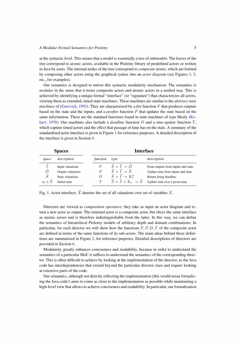
Our semantics is designed to mirror this syntactic modularity mechanism. The semantics ismodular in the sense that it treats composite actors and atomic actors in a unified way. This isachieved by identifying a unique formal “interface” (or “signature”) that characterizes all actors,viewing them as extended, timed state machines. These machines are similar to the abstract statemachines of (Gurevich, 1993). They are characterized by a fire function F that produces outputsbased on the state and the inputs, and a postfire function P that updates the state based on thesame information. These are the standard functions found in state machines of type Mealy (Ko-havi, 1978). Our machines also include a deadline function D and a time-update function T ,which capture timed actors and the effect that passage of time has on the state. A summary of thestandardized actor interface is given in Figure 1 for reference purposes. A detailed description ofthe interface is given in Section 4.

Spacesspace description

I Input valuations

O Output valuations

S State valuations

s0 ∈ S Initial state

Interfacefunction type description

F S × I → O Form outputs from inputs and state.

P S × I → S Update state from inputs and state.

D S × I → R∞+ Return firing deadline.

T S × I × R+ → S Update state over a given time.

Fig. 1. Actor interface: X denotes the set of all valuations over set of variables X .

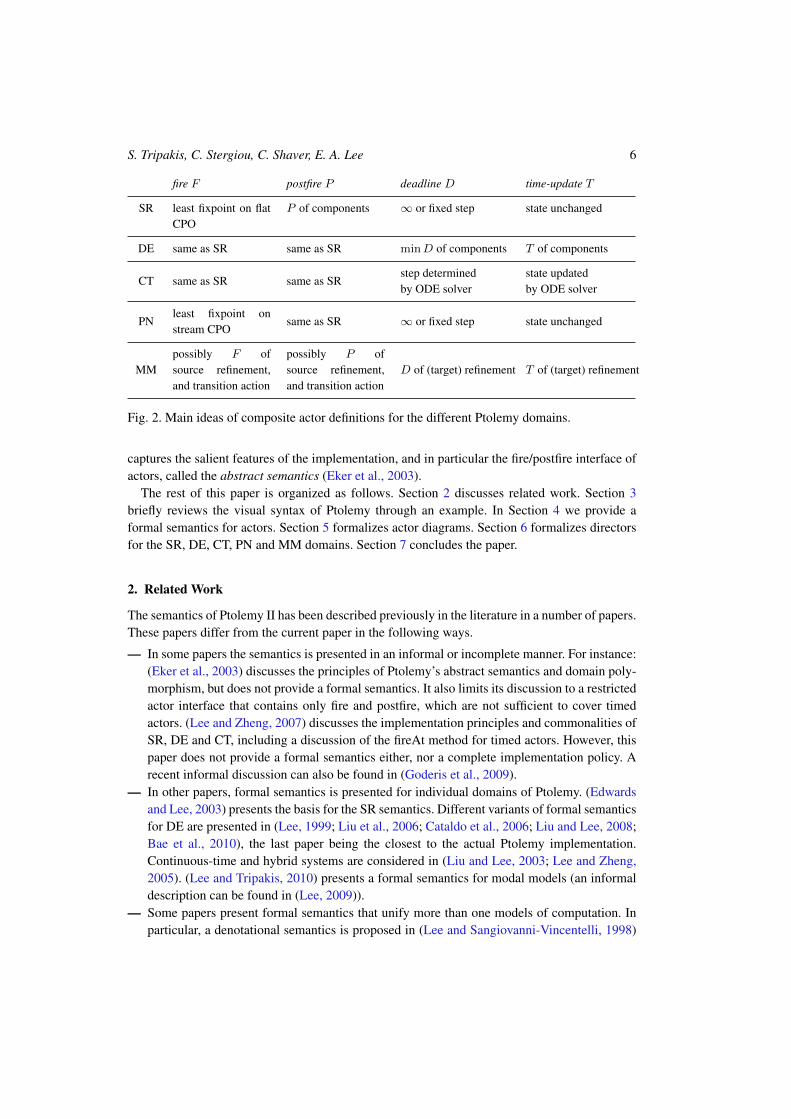
Directors are viewed as composition operators: they take as input an actor diagram and re-turn a new actor as output. The returned actor is a composite actor, but obeys the same interfaceas atomic actors and is therefore indistinguishable from the latter. In this way, we can definethe semantics of hierarchical Ptolemy models of arbitrary depth and domain combinations. Inparticular, for each director we will show how the functions F, P,D, T of the composite actorare defined in terms of the same functions of its sub-actors. The main ideas behind these defini-tions are summarized in Figure 2, for reference purposes. Detailed descriptions of directors areprovided in Section 6.

Modularity greatly enhances conciseness and readability, because in order to understand thesemantics of a particular MoC it suffices to understand the semantics of the corresponding direc-tor. This is often difficult to achieve by looking at the implementation of the director, as the Javacode has interdependencies that extend beyond the particular director class and require lookingat extensive parts of the code.

Our semantics, although not directly reflecting the implementation (this would mean formaliz-ing the Java code!) aims to come as close to the implementation as possible while maintaining ahigh-level view that allows to achieve conciseness and readability. In particular, our formalization

S. Tripakis, C. Stergiou, C. Shaver, E. A. Lee 6

fire F postfire P deadline D time-update T

SR least fixpoint on flatCPO

P of components ∞ or fixed step state unchanged

DE same as SR same as SR minD of components T of components

CT same as SR same as SRstep determined state updatedby ODE solver by ODE solver

PNleast fixpoint onstream CPO

same as SR ∞ or fixed step state unchanged

MMpossibly F ofsource refinement,and transition action

possibly P ofsource refinement,and transition action

D of (target) refinement T of (target) refinement

Fig. 2. Main ideas of composite actor definitions for the different Ptolemy domains.

captures the salient features of the implementation, and in particular the fire/postfire interface ofactors, called the abstract semantics (Eker et al., 2003).

The rest of this paper is organized as follows. Section 2 discusses related work. Section 3briefly reviews the visual syntax of Ptolemy through an example. In Section 4 we provide aformal semantics for actors. Section 5 formalizes actor diagrams. Section 6 formalizes directorsfor the SR, DE, CT, PN and MM domains. Section 7 concludes the paper.

2. Related Work

The semantics of Ptolemy II has been described previously in the literature in a number of papers.These papers differ from the current paper in the following ways.

— In some papers the semantics is presented in an informal or incomplete manner. For instance:(Eker et al., 2003) discusses the principles of Ptolemy’s abstract semantics and domain poly-morphism, but does not provide a formal semantics. It also limits its discussion to a restrictedactor interface that contains only fire and postfire, which are not sufficient to cover timedactors. (Lee and Zheng, 2007) discusses the implementation principles and commonalities ofSR, DE and CT, including a discussion of the fireAt method for timed actors. However, thispaper does not provide a formal semantics either, nor a complete implementation policy. Arecent informal discussion can also be found in (Goderis et al., 2009).

— In other papers, formal semantics is presented for individual domains of Ptolemy. (Edwardsand Lee, 2003) presents the basis for the SR semantics. Different variants of formal semanticsfor DE are presented in (Lee, 1999; Liu et al., 2006; Cataldo et al., 2006; Liu and Lee, 2008;Bae et al., 2010), the last paper being the closest to the actual Ptolemy implementation.Continuous-time and hybrid systems are considered in (Liu and Lee, 2003; Lee and Zheng,2005). (Lee and Tripakis, 2010) presents a formal semantics for modal models (an informaldescription can be found in (Lee, 2009)).

— Some papers present formal semantics that unify more than one models of computation. Inparticular, a denotational semantics is proposed in (Lee and Sangiovanni-Vincentelli, 1998)

A Modular Formal Semantics for Ptolemy 7

where processes are seen as relations between signals, where a signal is a set of taggedevents (events with timestamps in some abstract time domain). Only a single compositionoperator, essentially based on intersection, is provided. It is difficult to see how this cancapture different domains which, as mentioned above, are viewed as different compositionoperators in this paper.Another denotational semantics is proposed in (Liu and Lee, 2008), based on fixpoints onCPOs with a prefix order. This allows this semantics to be applied directly to a number ofdomains that can be naturally described using CPOs, in particular SR (Edwards and Lee,2003) and PN (Kahn, 1974). The authors also show how to incorporate timed systems (e.g.,DE) in the same framework. A similar denotational semantics is proposed in (Benvenisteet al., 2009) with the difference that a special “absent” value is not used.9 It is unclear howthis work can be extended to include other MoCs, in particular continuous-time and modalmodels.Finally, an abstract framework reminiscent of trace theory (Dill, 1988) is provided in (Burchet al., 2001). The latter can be seen as a “meta-framework” under which the heterogeneouscomposition of specific MoCs can be formulated, but does not include such formulations forthe MoCs considered in this paper.

An additional concern with some (although by no means all) of the above papers is also howclose the formal semantics is to the actual tool implementation. This is particularly a concernwith papers that present denotational semantics. Although we do not pretend in this paper topresent a semantics that exactly captures the tool implementation, we believe our semantics ismuch closer to the implementation than in previous works.

Aside from the above literature, most of which focuses on the Ptolemy tool in particular, arich body of research is concerned with the semantics of the individual MoCs considered in thispaper. Our work builds upon all this previous work, our focus being to develop a composablesemantics that integrates multiple models of computation. We next list the relations of our workto the previous work for each of the MoCs considered in this paper.

The semantics of SR is strongly related to those of the synchronous languages (Benvenisteand Berry, 1991; Halbwachs et al., 1991; Benveniste et al., 2003), and in particular the idea ofconstructive semantics of Esterel (Malik, 1994; Berry, 1996; Shiple et al., 1996). These ideashave been adapted in (Edwards and Lee, 2003) for a block-diagram notation, which is also theone used in Ptolemy in the case of SR. Our semantics follows the one of (Edwards and Lee, 2003)and extends it to “open” systems, in the sense that a composite block can have inputs. The theoryof fixpoints of Scott-continuous functions on CPOs (complete partial orders) is used to give anunambiguous meaning to models with feedback loops. Feedback loops may result in causalitycycles, but these are resolved by adding a special “bottom” value ⊥ representing an unknownvalue. As a result, the set of values becomes a “flat” CPO with ⊥ being the smallest element andall other values being incomparable. A monotonic function in this CPO is guaranteed to have aunique least fixpoint, and this is defined to be the semantics of a model.

9 This results in some loss of expressiveness, attested by the fact that the Adder actor cannot be specified in a satisfac-tory manner.

S. Tripakis, C. Stergiou, C. Shaver, E. A. Lee 8

The semantics of PN is based on Kahn Process Networks (Kahn, 1974). This semantics isalso given in terms of the least fixpoint of a continuous function on a CPO, however, the CPO isdifferent here than the one used in SR. In SR, inputs and outputs are individual values, whereasin PN they are streams, i.e., finite or infinite sequences of values. Streams are ordered with theprefix order, and the empty sequence is the minimal element of the corresponding CPO. Thestream CPO is not flat, in fact, it has infinite height (since finite streams can be of arbitrarylength). As a result, monotonicity of functions does not generally imply Scott-continuity. Scott-continuity is a reasonable assumption to make, however, and it is satisfied by actors in practice.

The PN semantics is a denotational semantics. The stream CPO has infinite height, therefore,the least fixpoint may not be reachable in a finite number of iterations. In fact, problems suchas deciding whether in a given PN model the length of a produced stream is finite are undecid-able (Buck, 1993). Algorithmic ways of executing a PN model that satisfy different propertiesare provided in (Lee and Parks, 1995) and (Geilen and Basten, 2003). The semantics of PN isunified with the semantics of dataflow models in (Lee and Matsikoudis, 2009). Reactive processnetworks which extend process networks with event-based control are defined in (Geilen andBasten, 2004).

The semantics of DE has been an old topic of discussion (Reed and Roscoe, 1988; Yates,1993), which is also related to fixpoint semantics based on metric spaces or CPOs (Arnold andNivat, 1980; Baier and Majster-Cederbaum, 1994). The DE domain is related to other modelsof computation that have a dense-time semantics. An example is timed automata (Alur and Dill,1994). A timed automaton has a finite number of clocks, whereas in DE a separate clock may berequired for each token, which makes the number of clocks a-priori unbounded. For this reason,DE models are not directly representable as timed automata. They could be representable as someform of timed Petri nets (Sifakis, 1977) but to our knowledge, this link has not been explored yet.

SR, PN and DE have semantical similarities that have been explored and exploited in the liter-ature (Broy and Stolen, 2001; Liu and Lee, 2008; Benveniste et al., 2009). Particularly relevantis the work on FOCUS (Broy and Stolen, 2001) which offers a general framework for specifyingsystems based on stream-processing elements. FOCUS can capture both untimed and timed sys-tems, as well as asynchronous and synchronous systems. It provides formal refinement relationsand guarantees of compositionality.

The semantics of CT is based on numerical methods for solving differential equations. Combi-nations of CT models with discrete logic (e.g., modal models) result in models similar to hybridsystems (Manna and Pnueli, 1992). The faithful reproduction of the semantics of such systemsby a computer, for instance, by simulation, is a difficult problem and still an active area of re-search (e.g., see (Zhu et al., 2010)). (Liu and Lee, 2003) uses the notion of an ideal solver, whichcan solve a set of differential equations exactly, provided the equations satisfy a Lipschitz condi-tion over a given time interval. This is not as far-fetched as it might sound, because closed formexpressions can sometimes be given for the solution over the intervals of continuous behavior.Even when we do not have closed form solutions, for many special cases, numerical solutionsyield exact answers (using appropriate solvers). But even in cases where the solution must beapproximated, it is valuable to separate the issue of approximate ODE solutions from the othersemantic issues (such as determinacy of the model). Hence, the idealization remains useful.

Modal models are based on hierarchical state machines, various versions of which have beenstudied in the literature or are available as commercial products, including Statecharts (Harel,

A Modular Formal Semantics for Ptolemy 9

1987), SyncCharts (André, 1996), Stateflow from the Mathworks, Safe State Machines from Es-terel Technologies (André, 2003) (SSMs are based on SyncCharts), and UML state machines.A variety of different semantics has been proposed for Statecharts for instance, see (Beeck,1994; Eshuis, 2009). Some of these semantics are synchronous in nature. SyncCharts also uses asynchronous semantics. An alternative for incorporating mode switching into synchronous lan-guages is presented in (Maraninchi and Rémond, 2003). The semantics of Stateflow are based onthe “run-to-completion” principle which is not really synchronous, although it can be approxi-mated by a synchronous model (Scaife et al., 2004). Operational and denotational semantics forStateflow are presented in (Hamon and Rushby, 2004; Hamon, 2005). Timed versions of State-charts and UML have been proposed in (Damm et al., 1998; Graf et al., 2006). In Ptolemy modalmodels the hierarchy is not restricted to contain only state machines or concurrent state machines(built with AND states). Also, contrary to Statecharts, SyncCharts and Stateflow, Ptolemy modalmodels do not use broadcast events for communication. Instead, communication is done viaports, as in the block-diagram based notation of Ptolemy.

A number of other modeling frameworks exist that provide mechanisms for mixing MoCs. Anearly systematic approach to such mixed models was realized in Ptolemy Classic (Buck et al.,1994). The Metropolis environment (Balarin et al., 2003; Goessler and Sangiovanni-Vincentelli,2002) focuses on modeling both function and architecture, as well as the mapping of the formerto the latter. Metropolis includes the concepts of constraints and quantity managers that are usedto constrain the behaviors of a model and annotate them with quantities such as time, energyor other metrics. The Generic Modeling Environment (GME) (Karsai, 1995; Nordstrom et al.,1999; Ledeczi et al., 2001) uses metamodeling techniques to create domain-specific modelingand program synthesis environments. BIP (Basu et al., 2006; Bliudze and Sifakis, 2008a; Bozgaet al., 2009) models are built by composing behavioral components with n-ary rendezvous basedinteractions and then restricting those interactions using priorities. An important problem that re-searchers working on BIP have tackled is that of glue expressiveness, namely, what is the relativeexpressive power of two modeling formalisms with same sets of basic components but differ-ent composition operators (Bliudze and Sifakis, 2008b). Specifying interaction as a first-classcitizen is also at the heart of the Reo model of concurrency (Arbab, 2004). In Reo, complexinteraction protocols (connectors) can be formed by combining simpler protocols (channels),such as bounded/unbounded and lossless/lossy versions of FIFO queues. Composition is per-formed by creating channels and connecting their end-points in a graph-oriented manner usingoperators such as join or split. Glue expressiveness has been studied in the context of Reo aswell: (Arbab, 2004) shows examples of how protocols that can be expressed as regular expres-sions over I/O operations can also be captured by Reo connectors composed of five primitivechannels. The ModHel’X environment (Hardebolle et al., 2007; Boulanger et al., 2011) shares anumber of concepts with Ptolemy, such as hierchical composition of MoCs, and emphasizes theuse of interface blocks that perform “semantic adaptation” between heterogeneous models. Forinstance, when embedding an SDF model within a DE model, an interface block can be used toadd timestamps to the typically untimed outputs of SDF. ForSyDe (Jantsch, 2003; Sander andJantsch, 2004) provides a set of libraries for capturing heterogeneous MoCs based on the func-tional programming language Haskell. ForSyDe includes different model transformations thatare used to refine an abstract specification model into a detailed implementation model, whichcan be translated into a target implementation language. SystemC is capable of realizing multiple

S. Tripakis, C. Stergiou, C. Shaver, E. A. Lee 10

MoCs with a discrete-event simulation flavor (Patel and Shukla, 2004; Herrera and Villar, 2006).An interesting way of expressing the semantics of a MoC is given by “42” (Maraninchi andBhouhadiba, 2007), which integrates with an application model a specification of a customizedMoC. A mechanism to create domain-polymorphic components similar in spirit to Ptolemy isproposed in (Feredj et al., 2009). Close in spirit to this paper are also the works (Bliudze andKrob, 2009; Aiguier et al., 2011), whose goal is to provide a sound semantical framework forheterogeneous systems, in particular with respect to the integration of systems operating at dif-ferent time dimensions and scales. In (Bliudze and Krob, 2009) a system (in our terms, actor)is captured as a kind of timed Turing machine, where non-standard analysis is used to representcontinuous time via infinitesimals. In (Aiguier et al., 2011) a system is captured as a kind of timedMealy machine. The interface of these machines contains two functions, an output function and astate-update function, as in a Mealy machine, except that time is an additional input argument toboth functions. Composition in this framework is achieved by three operators: parallel composi-tion, feedback and abstraction. Therefore, in the approach of (Aiguier et al., 2011), the differentMoCs are not realized by the composition operators (as is the case with Ptolemy).

Perhaps the work most closely related to our paper is (Denckla and Mosterman, 2008). There,the authors present two types of semantics for a block-diagram language with hierarchy: astream-based semantics where blocks are viewed as functions from streams to streams; and astate-based semantics where each block is represented by an initial state and a kind of ‘step’function which, given the current input and state, returns the current output and an ‘implicit out-put’. For discrete systems the latter is interpreted as ‘next state’, whereas for continuous systemsit is interpreted as the time derivative of the state. A solver is then used to transform continuoussystems to discrete systems. The state-based semantics of (Denckla and Mosterman, 2008) isclosely related to the semantics we present in this paper. However, the (single) step function usedthere is different from our 4-function actor interface. In particular, their step function does notappear to be able to explicitly manipulate time (e.g., to specify a deadline).

Comparing the above frameworks among themselves as well as with Ptolemy, stating preciselythe strengths and weaknesses of each, is a difficult task. This is partly because each of the aboveprojects pursues slightly different goals, ranging from “pure” modeling and simulation, to verifi-cation, to design-space exploration, mapping and implementation. Ptolemy focuses on modelingand simulation, and leverages external tools (e.g., model-checkers) and code-generators for othertasks (e.g., verification).

In terms of expressiveness, many frameworks are equivalent in the sense of being Turing-complete. However, other types of expressiveness may be more appropriate in the context ofheterogeneous modeling, such as glue expressiveness (Bliudze and Sifakis, 2008b). A formalcomparison of the semantics of Ptolemy viewed as a kind of “glue” and compared to other gluesis beyond the scope of this paper, but a worth-pursuing future research direction.

Another, perhaps a more fundamental issue is that modeling and design are ultimately creativetasks and therefore inherently subjective to human taste, experience, and other factors. Whichtypes of designs are easier to build or more intuitive to understand in each of the above ap-proaches? This is at least as difficult as the question: which kind of programs are easier to writein each of the existing programming languages. Most designs could in principle be capturedin any of the frameworks listed above, and even in homogeneous modeling frameworks, usingclever encodings. The question is how much effort is required to do so, as well as to understand

A Modular Formal Semantics for Ptolemy 11

the result, modify it when necessary, use it for analysis or implementation, and so on. Ptolemystrives to offer a framework which is as general as possible (integrating many MoCs), yet at thesame time as intuitive as possible, so that an individual model written in, say, SDF or CT, behavesin Ptolemy as one familiar with SDF or CT would expect it to behave.

Finally, a number of component-oriented frameworks come from the fields of traditional pro-gramming and software engineering, e.g., object-oriented programming languages such as Eif-fel (Meyer, 1992), component diagrams in UML and other notations, and component modelssuch as CORBA CCM, .NET, EJB, or Fractal (Bruneton et al., 2006), to name a few. The com-mon characteristic that these frameworks have with ours is that they also provide notions ofstandardized interfaces, from the level of notation, as with UML-based frameworks, to the levelof execution, as with concrete implementations of frameworks like Fractal. The above frame-works have a variety of objectives, which are quite different from ours. Our main goal is to comeup with the right actor interface to express the behavioral semantics of many different MoCs.

3. Ptolemy’s Graphical Syntax

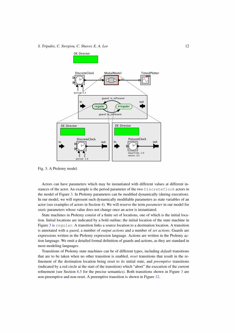
Before presenting the formal semantics, we give a brief overview of Ptolemy’s graphical syntax,via an example, shown in Figure 3. There are 9 actors in this model:

1 The top-level actor is a composite actor, composed with the DE director. This top-level actorcontains three sub-actors.

2 The DiscreteClock actor with period 2.5 embedded in the top-level actor.3 The TimedPlotter actor embedded in the top-level actor.4 The ModalModel actor embedded in the top-level actor. The ModalModel actor is also a

composite actor, composed with the MM director.5 The controller automaton of the ModalModel actor, which has two locations, regular

and irregular.10

6 The composite actor refining state regular of ModalModel. This composite actor is com-posed with the DE director.

7 The composite actor refining state irregular of ModalModel. This composite actor iscomposed with the DE director.

8 The DiscreteClock actor with period 1.0 embedded in the composite actor refiningregular.

9 The PoissonClock actor embedded in the composite actor refining irregular.

Out of these 9 actors, 4 are composite actors and 5 are atomic actors.11 Each composite actoris associated with an actor diagram, therefore, the model also contains 4 actor diagrams.

Actors in Ptolemy have ports, rendered graphically as small triangles attached to the “boxes”that represent the external view of actors. In composite actors, ports appear also internally in thecorresponding actor diagram. Ports can be input or output. For example, DiscreteClock hasfour input ports and one output port. ModalModel has one input port and one output port.

10 For state machines and modal models, we use the term location instead of state, in order to distinguish it from thesemantical concept of state (defined formally in Section 4).

11 We classify the automaton of the modal model as an atomic actor. It could also be classified as a composite actor,composed from basic states and transitions, but this would make things more complex than necessary.

S. Tripakis, C. Stergiou, C. Shaver, E. A. Lee 12

Fig. 3. A Ptolemy model.

Actors can have parameters which may be instantiated with different values at different in-stances of the actor. An example is the period parameter of the two DiscreteClock actors inthe model of Figure 3. In Ptolemy parameters can be modified dynamically (during execution).In our model, we will represent such dynamically modifiable parameters as state variables of anactor (see examples of actors in Section 4). We will reserve the term parameter in our model forstatic parameters whose value does not change once an actor is instantiated.

State machines in Ptolemy consist of a finite set of locations, one of which is the initial loca-tion. Initial locations are indicated by a bold outline; the initial location of the state machine inFigure 3 is regular. A transition links a source location to a destination location. A transitionis annotated with a guard, a number of output actions and a number of set actions. Guards areexpressions written in the Ptolemy expression language. Actions are written in the Ptolemy ac-tion language. We omit a detailed formal definition of guards and actions, as they are standard inmost modeling languages.

Transitions of Ptolemy state machines can be of different types, including default transitionsthat are to be taken when no other transition is enabled, reset transitions that result in the re-finement of the destination location being reset to its initial state, and preemptive transitions(indicated by a red circle at the start of the transition) which “abort” the execution of the currentrefinement (see Section 6.5 for the precise semantics). Both transitions shown in Figure 3 arenon-preemptive and non-reset. A preemptive transition is shown in Figure 12.

A Modular Formal Semantics for Ptolemy 13

Briefly, the behavior of the model of Figure 3 is that the ModalModel actor switches be-tween two modes of operation every 2.5 time units: in the regular mode it generates aregularly-spaced clock signal while in the irregular mode, it generates pseudo-randomlyspaced events, as illustrated in Figure 11. See Section 6.5 for a more detailed description of thebehavior of this model.

4. Actors

4.1. Variables, Assignments and Timers

Let S be a set of variables (more precisely, variable names). We will assume that all variables takevalues in some universe of values U . A valuation (or assignment) over S is a function x : S → Uthat assigns to each variable v ∈ S some value x(v) ∈ U . The set of all assignments over S isdenoted S. Note that if S1 and S2 are disjoint sets of variables, then S1 ∪ S2 is isomorphic toS1 × S2. If x1 ∈ S1 and x2 ∈ S2 we write (x1, x2) for the valuation x ∈ S1 ∪ S2 such thatx(v1) = x1(v1) for all v1 ∈ S1 and x(v2) = x2(v2) for all v2 ∈ S2. If S′ ⊆ S and x ∈ S

then x �S′ is the restriction (or projection) of x to S′, that is, the valuation x′ ∈ S′ such thatx′(v) = x(v) for all v ∈ S′.

We use the following notation for valuations. If x ∈ S, v ∈ S, and α ∈ U , then {x | v 7→ α}denotes the new valuation x′ obtained from x by setting v to α and leaving other variablesunchanged. A new valuation is denoted by listing the assignments for all variables in S. Forexample, if S = {v1, v2} and α1, α2 ∈ U , then {v1 7→ α1, v2 7→ α2} denotes the valuationx ∈ S such that x(v1) = α1 and x(v2) = α2.

We will often use a special type of variables called timers. Timers are implicitly typed to takevalues in R+, the set of non-negative real numbers. We use R∞+ to denote the set R+ ∪ {∞},where∞ denotes (positive) infinity.

Two special values in U are⊥, representing “bottom” or “unknown”, and absent, representingthe “absence” of a signal at a particular point in time. Unknown values are useful when definingthe semantics of diagrams of actors that contain feedback loops, as the fixpoint of some function.We define such fixpoint semantics for SR, DE and CT (see Sections 6.1, 6.2 and 6.3). Absentvalues are useful in models with discrete events, where at any given time either an event occursor it does not: in the former case, the corresponding signal is present (and assumes some value),whereas in the latter case, the signal has value absent. Note that the concepts of absent and un-known are very different. A signal that takes absent values is perfectly legal in a model. However,a signal that is sometimes unknown corresponds to a “bad”, ambiguous model. In the rest of thepaper we present concrete examples of actors and models that manipulate these values.

4.2. Actors

An actor is a tuple

A = (I,O, S, s0, F, P,D, T ) (1)

S. Tripakis, C. Stergiou, C. Shaver, E. A. Lee 14

where I is a set of input variables, O is a set of output variables,12 S is a set of state variables,s0 ∈ S is a valuation over S representing the initial state, and F, P,D, T are total functions withthe following types:

F : S × I → O (2)

P : S × I → S (3)

D : S × I → R∞+ (4)

T : S × I × R+ → S (5)

We assume that I,O, S are pair-wise disjoint, i.e., I ∩ O = I ∩ S = O ∩ S = ∅. We use theterms input, output, state to mean valuations over I,O, S, respectively. For example, x : I → Uis an input, y : O → U is an output, and s : S → U is a state.

Note that any of the sets of variables I,O, S may be empty or infinite. By convention, the setof valuations over an empty set of variables is a singleton, i.e., a set with a single element that wewill denote ∗. Even if all its sets of variables are finite, an actor need not be finite-state, since itsstate space, i.e., S, can still be infinite. This is because the domains of variables can be infinite.Similarly, the input and output spaces can be infinite.F, P,D and T are called the fire, postfire, deadline and time-update functions of A, respec-

tively. F and P are similar to the output and transition functions of a state machine. F producesan output given a state and an input. P produces a new state, given the same information as F .D returns a deadline, indicating how much time the actor is willing to let elapse. T updates thestate given information on the actual delay chosen by the environment. Delays and deadlines areuseful to model the semantics of timed actors. Their role should become clear when we explaintimed behaviors below.

4.3. Actor Behaviors

An actor A = (I,O, S, s0, F, P,D, T ) defines a set of behaviors. Our model of behaviors isinspired from the semantic models of timed or hybrid automata (Alur et al., 1995). A timedbehavior of A is a sequence

s0

x0/y0 // s′0x′0/d0 // s1

x1/y1 // s′1x′1/d1 // s2

x2/y2 // s′2x′2/d2 // · · · (6)

where for all i ∈ N, si, s′i ∈ S, di ∈ R+, xi ∈ I , yi ∈ O, and

yi = F (si, xi) (7)

s′i = P (si, xi) (8)

di ≤ D(s′i, x′i) (9)

si+1 = T (s′i, x′i, di) (10)

The intuition is as follows. Suppose that at some point in time, say t ∈ R+, A is at state si.The environment provides input xi to A and A instantaneously produces output yi using its F

12 In Ptolemy terminology, the term ports is used for input and output variables.

A Modular Formal Semantics for Ptolemy 15

function, and moves to state s′i using its P function. The environment then proposes to advancetime and “asks” A whether it has any restrictions on the amount of time that may elapse. A“replies” by returning a deadline D(s′i, x

′i) on the amount of time that may elapse. To compute

this deadline, A may in general use input value x′i which is provided by the environment. Thisvalue can be viewed as an estimate of the environment of the value of input variables during thenext interval of time. Next, the environment chooses to advance time by some concrete delay di ∈R+, making sure that di does not violate the deadline provided by A. Finally, the environmentnotifies A that it advanced time by di and A updates its state to si+1 accordingly, using its Tfunction. The new time is t+ di and execution repeats from then on in the same fashion.

It is worth noting that in our model of actors and behaviors, the “interesting points in time”are determined by the environment, and not the actor. In fact, the actor has no explicit notion oftime (although it can measure time by using state variables, e.g., timers). However, the actor canimpose constraints on the advancement of time using deadlines.

The fact that F, P,D, T are functions makes our actors deterministic. This is done for reasonsof simplicity, and because our main focus is heterogeneity. Non-deterministic actors could bemodeled, however, as deterministic actors using extra input variables.

4.4. Actor Classification and Special Cases

Consider an actor A = (I,O, S, s0, F, P,D, T ).

— A is called a source if it has no input variables, i.e., I = ∅.— A is called a sink if it has no output variables, i.e., O = ∅.— A is called stateless if it has no state variables, i.e., S = ∅.— A is called untimed if D is a constant function that always returns infinity, i.e., for any state

s and input x, D(s, x) =∞. Otherwise A is called timed.— A is called delay-independent if T leaves the state unchanged, i.e., for any state s, input x,

and delay d, T (s, x, d) = s. Otherwise A is called delay-dependent.— A is called a dataflow actor if its input and output variables range over streams.

When a set of variables is empty or a function is independent of one or more of its parameters,the type of the function simplifies, and we accordingly simplify our notation. For instance, if Ais a source then I is a singleton, therefore, F does not depend on the input. Because of this, wecan assume that F is a function with a simpler type F : S → O and we can write F (s), for states. We similarly simplify notation for other special cases of actors. For example, for a statelessactor, we write F (x), for input x. For an actor that is both stateless and a source, we write F ().Also note that for a stateless actor functions P and T are trivial: they are the constant functionsthat return the unique element ∗, therefore they need not be specified.

4.5. Examples of Atomic Actors

4.5.1. Constant: The Constant actor parameterized by some value α ∈ U is an actor that intu-itively produces the constant value α every time it is fired. This actor can be modeled as follows:

Constα = (∅, {o}, ∅, ∗, F, P,D, T ) (11)

S. Tripakis, C. Stergiou, C. Shaver, E. A. Lee 16

where

F () = {o 7→ α} and D() =∞ (12)

F returns the valuation y ∈ {o} which assigns α to the unique output variable o. Constα is asource, and it is also stateless, untimed, and delay-independent.

4.5.2. Identity: The Identity actor simply “copies” its input to its output. This actor can be mod-eled as follows:

Id = ({v}, {o}, ∅, ∗, F, P,D, T ) (13)

where

F (x) = {o 7→ x(v)} and D(x) =∞ (14)

for any input x.F returns the valuation y ∈ {o} which assigns to the unique output variable o the value x(v)

of the unique input variable v at the input valuation x. Id is a stateless, untimed, and delay-independent actor.

4.5.3. Adder: The Adder actor intuitively produces a value that corresponds to the sum of itsinputs every time it is fired. This actor can be modeled as follows:

Add = ({v1, v2}, {o}, ∅, ∗, F, P,D, T ) (15)

where

F (x) =

{{o 7→ (x(v1)⊕ x(v2))} if x(v1) 6= ⊥ and x(v2) 6= ⊥{o 7→ ⊥} otherwise

(16)

u1 ⊕ u2 =

u1 + u2 if u1 6= absent and u2 6= absent

u1 if u1 6= absent and u2 = absent

u2 if u1 = absent and u2 6= absent

absent if u1 = absent and u2 = absent

(17)

D(x) = ∞ (18)

for any input x. That is, F returns the valuation y ∈ {o} which assigns to the unique outputvariable o the sum x(v1) + x(v2) of the values of the two input variables v1 and v2, providednone of these values are unknown (i.e., ⊥), or absent. If any of the input values is unknown, theoutput is unknown. If one of the inputs is absent, the output is equal to the other input. If bothinputs are absent, the output is absent.Add is stateless, untimed and delay-independent.

4.5.4. Logical-and: The And actor intuitively produces a value that corresponds to the logical-and (conjunction) of its inputs every time it is fired. This actor can be modeled as follows:

And = ({v1, v2}, {o}, ∅, ∗, F, P,D, T ) (19)

A Modular Formal Semantics for Ptolemy 17

where

F (x) =

{o 7→ false} if x(v1) = false or x(v2) = false

{o 7→ true} if x(v1) = true and x(v2) = true, otherwise:{o 7→ x(v1)} if x(v2) = absent

{o 7→ x(v2)} if x(v1) = absent

{o 7→ ⊥} otherwise

(20)

D(x) = ∞ (21)

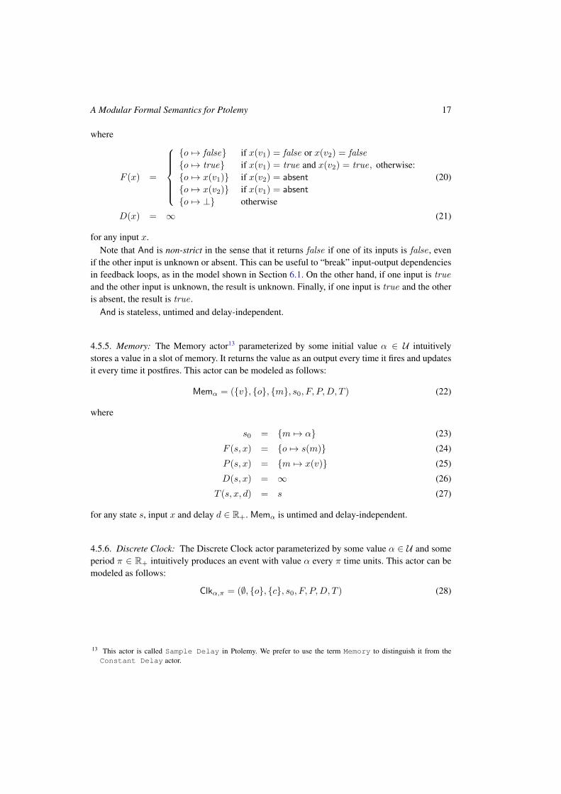
for any input x.Note that And is non-strict in the sense that it returns false if one of its inputs is false , even

if the other input is unknown or absent. This can be useful to “break” input-output dependenciesin feedback loops, as in the model shown in Section 6.1. On the other hand, if one input is trueand the other input is unknown, the result is unknown. Finally, if one input is true and the otheris absent, the result is true .And is stateless, untimed and delay-independent.

4.5.5. Memory: The Memory actor13 parameterized by some initial value α ∈ U intuitivelystores a value in a slot of memory. It returns the value as an output every time it fires and updatesit every time it postfires. This actor can be modeled as follows:

Memα = ({v}, {o}, {m}, s0, F, P,D, T ) (22)

where

s0 = {m 7→ α} (23)

F (s, x) = {o 7→ s(m)} (24)

P (s, x) = {m 7→ x(v)} (25)

D(s, x) = ∞ (26)

T (s, x, d) = s (27)

for any state s, input x and delay d ∈ R+. Memα is untimed and delay-independent.

4.5.6. Discrete Clock: The Discrete Clock actor parameterized by some value α ∈ U and someperiod π ∈ R+ intuitively produces an event with value α every π time units. This actor can bemodeled as follows:

Clkα,π = (∅, {o}, {c}, s0, F, P,D, T ) (28)

13 This actor is called Sample Delay in Ptolemy. We prefer to use the term Memory to distinguish it from theConstant Delay actor.

S. Tripakis, C. Stergiou, C. Shaver, E. A. Lee 18

where

s0 = {c 7→ 0} (29)

F (s) =

{{o 7→ α} if s(c) = 0

{o 7→ absent} otherwise(30)

P (s) =

{{c 7→ π} if s(c) = 0

{c 7→ s(c)} otherwise(31)

D(s) = s(c) (32)

T (s, d) = {c 7→(s(c)− d

)} (33)

for any state s, and delay d ∈ R+ such that d ≤ D(s).

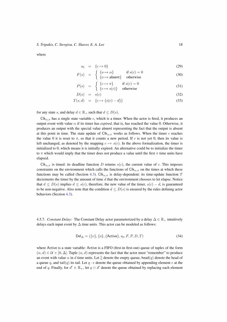
Clkα,π has a single state variable c, which is a timer. When the actor is fired, it produces anoutput event with value α if its timer has expired, that is, has reached the value 0. Otherwise, itproduces an output with the special value absent representing the fact that the output is absentat this point in time. The state update of Clkα,π works as follows. When the timer c reachesthe value 0 it is reset to π, so that it counts a new period. If c is not yet 0, then its value isleft unchanged, as denoted by the mapping c 7→ s(c). In the above formalization, the timer isinitialized to 0, which means it is initially expired. An alternative could be to initialize the timerto π which would imply that the timer does not produce a value until the first π time units haveelapsed.

Clkα,π is timed: its deadline function D returns s(c), the current value of c. This imposesconstraints on the environment which calls the functions of Clkα,π on the times at which thesefunctions may be called (Section 4.3). Clkα,π is delay-dependent: its time-update function Tdecrements the timer by the amount of time d that the environment chooses to let elapse. Noticethat d ≤ D(s) implies d ≤ s(c), therefore, the new value of the timer, s(c) − d, is guaranteedto be non-negative. Also note that the condition d ≤ D(s) is ensured by the rules defining actorbehaviors (Section 4.3).

4.5.7. Constant Delay: The Constant Delay actor parameterized by a delay ∆ ∈ R+ intuitivelydelays each input event by ∆ time units. This actor can be modeled as follows:

Del∆ = ({v}, {o}, {Active}, s0, F, P,D, T ) (34)

where Active is a state variable: Active is a FIFO (first-in first-out) queue of tuples of the form(α, d) ∈ U × [0,∆]. Tuple (α, d) represents the fact that the actor must “remember” to producean event with value α in d time units. Let [] denote the empty queue, head(q) denote the head ofa queue q, and tail(q) its tail. Let q · e denote the queue obtained by appending element e at theend of q. Finally, for d′ ∈ R+, let q d′ denote the queue obtained by replacing each element

A Modular Formal Semantics for Ptolemy 19

(α, d) of q by (α, d− d′). Then, we have:

s0 = {Active 7→ []} (35)

F (s, x) =

{{o 7→ α} if s(Active) 6= [] and head(s(Active)) = (α, 0)

{o 7→ absent} otherwise(36)

P (s, x) =

{{Active 7→

(A′ · (α,∆)

)} if x(v) = α and α 6= absent

{Active 7→ A′} otherwise(37)

A′ =

{tail(s(Active)) if s(Active) 6= [] and head(s(Active)) = (α, 0)

s(Active) otherwise(38)

D(s, x) =

{d if s(Active) 6= [] and head(s(Active)) = (α, d)

∞ otherwise(39)

T (s, x, d) = {Active 7→(s(Active) d

)} (40)

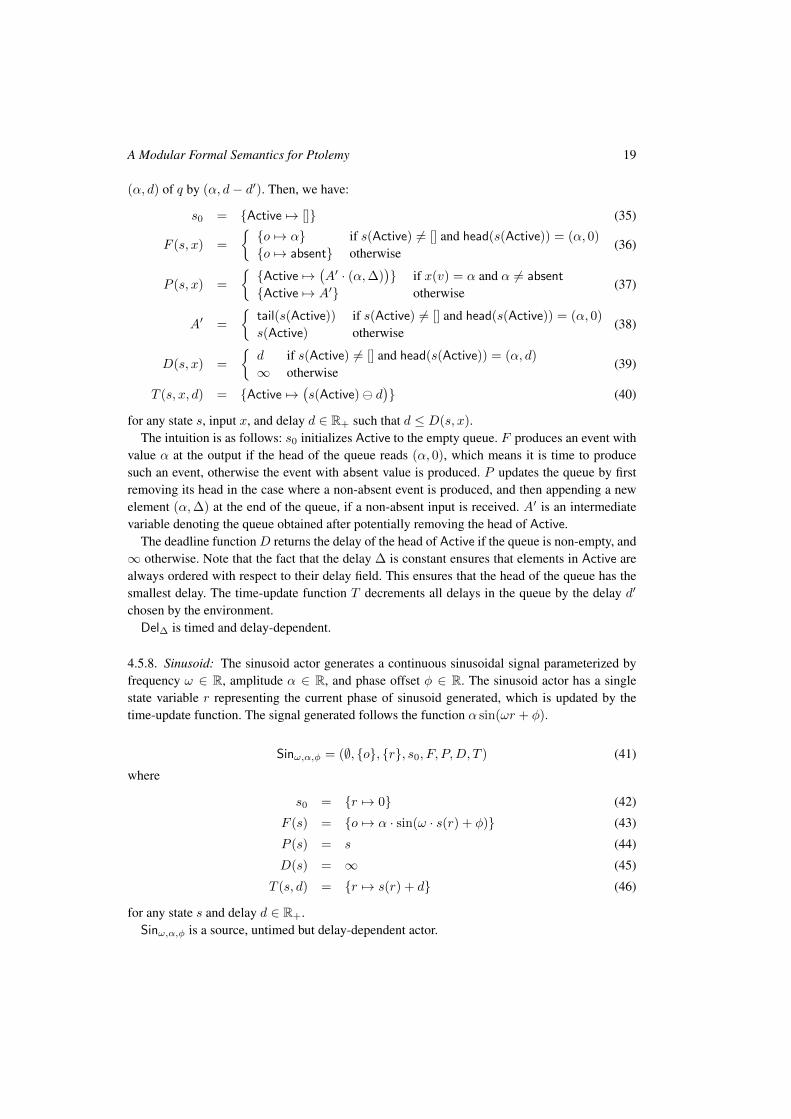
for any state s, input x, and delay d ∈ R+ such that d ≤ D(s, x).The intuition is as follows: s0 initializes Active to the empty queue. F produces an event with

value α at the output if the head of the queue reads (α, 0), which means it is time to producesuch an event, otherwise the event with absent value is produced. P updates the queue by firstremoving its head in the case where a non-absent event is produced, and then appending a newelement (α,∆) at the end of the queue, if a non-absent input is received. A′ is an intermediatevariable denoting the queue obtained after potentially removing the head of Active.

The deadline function D returns the delay of the head of Active if the queue is non-empty, and∞ otherwise. Note that the fact that the delay ∆ is constant ensures that elements in Active arealways ordered with respect to their delay field. This ensures that the head of the queue has thesmallest delay. The time-update function T decrements all delays in the queue by the delay d′

chosen by the environment.Del∆ is timed and delay-dependent.

4.5.8. Sinusoid: The sinusoid actor generates a continuous sinusoidal signal parameterized byfrequency ω ∈ R, amplitude α ∈ R, and phase offset φ ∈ R. The sinusoid actor has a singlestate variable r representing the current phase of sinusoid generated, which is updated by thetime-update function. The signal generated follows the function α sin(ωr + φ).

Sinω,α,φ = (∅, {o}, {r}, s0, F, P,D, T ) (41)

where

s0 = {r 7→ 0} (42)

F (s) = {o 7→ α · sin(ω · s(r) + φ)} (43)

P (s) = s (44)

D(s) = ∞ (45)

T (s, d) = {r 7→ s(r) + d} (46)

for any state s and delay d ∈ R+.Sinω,α,φ is a source, untimed but delay-dependent actor.

S. Tripakis, C. Stergiou, C. Shaver, E. A. Lee 20

4.5.9. Integrator: The Integrator actor Integratorα, parameterized by initial value α ∈ R+, isused by the CT director (Section 6.3) to perform integration. Integratorα is in fact identical toMemα. However, we use a special name as a syntactic mechanism that permits the CT directorto identify the integrator actors in a given model.

It may appear surprising that Integrators are nothing else but memories, but this is the case fornumerical solvers of Runge-Kutta type (see Section 6.3). Integrators would be less trivial undera different solver, for instance, a fixed-step Euler solver. In that case, Integrators can be definedto perform the integration, at the same time eliminating the need for a special CT director: in thecase of Euler integration, the DE director is sufficient.

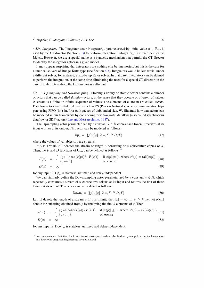
4.5.10. Upsampling and Downsampling: Ptolemy’s library of atomic actors contains a numberof actors that can be called dataflow actors, in the sense that they operate on streams of values.A stream is a finite or infinite sequence of values. The elements of a stream are called tokens.Dataflow actors are useful in domains such as PN (Process Networks) where communication hap-pens using FIFO (first-in, first-out) queues of unbounded size. We illustrate how data actors canbe modeled in our framework by considering first two static dataflow (also called synchronousdataflow or SDF) actors (Lee and Messerschmitt, 1987).

The Upsampling actor parameterized by a constant k ∈ N copies each token it receives at itsinput n times at its output. This actor can be modeled as follows:

Upn = ({p}, {q}, ∅, ∗, F, P,D, T ) (47)

where the values of variables p, q are streams.If α is a value, αn denotes the stream of length n consisting of n consecutive copies of α.

Then, the F and D functions of Upn can be defined as follows:14

F (x) =

{{q 7→ head(x(p))n · F (x′)} if x(p) 6= [], where x′(p) = tail(x(p))

{q 7→ []} otherwise(48)

D(x) = ∞ (49)

for any input x. Upn is stateless, untimed and delay-independent.We can similarly define the Downsampling actor parameterized by a constant n ∈ N, which

repeatedly consumes a stream of n consecutive tokens at its input and returns the first of thesetokens at its output. This actor can be modeled as follows:

Downn = ({p}, {q}, ∅, ∗, F, P,D, T ) (50)

Let |ρ| denote the length of a stream ρ. If ρ is infinite then |ρ| = ∞. If |ρ| ≥ k then let ρ(k..)

denote the substring obtained from ρ by removing the first k elements of ρ. Then:

F (x) =

{{q 7→ head(x(p)) · F (x′)} if |x(p)| ≥ n, where x′(p) = (x(p))(n..)

{q 7→ []} otherwise(51)

D(x) = ∞ (52)

for any input x. Downn is stateless, untimed and delay-independent.

14 we use a recursive definition for F as it is easier to express, and can also be directly mapped into an implementationin a functional programming language such as Haskell

A Modular Formal Semantics for Ptolemy 21

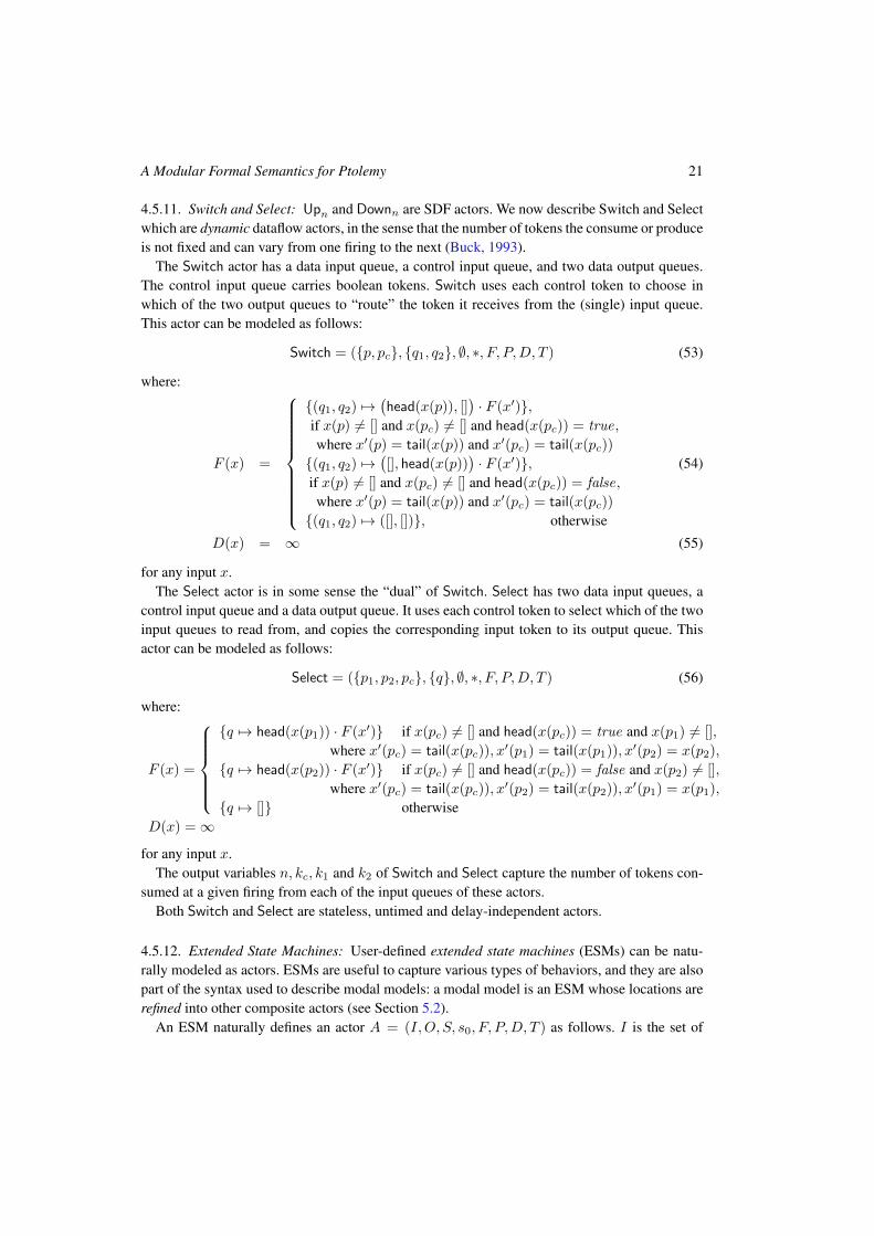
4.5.11. Switch and Select: Upn and Downn are SDF actors. We now describe Switch and Selectwhich are dynamic dataflow actors, in the sense that the number of tokens the consume or produceis not fixed and can vary from one firing to the next (Buck, 1993).

The Switch actor has a data input queue, a control input queue, and two data output queues.The control input queue carries boolean tokens. Switch uses each control token to choose inwhich of the two output queues to “route” the token it receives from the (single) input queue.This actor can be modeled as follows:

Switch = ({p, pc}, {q1, q2}, ∅, ∗, F, P,D, T ) (53)

where:

F (x) =

{(q1, q2) 7→(head(x(p)), []

)· F (x′)},

if x(p) 6= [] and x(pc) 6= [] and head(x(pc)) = true,

where x′(p) = tail(x(p)) and x′(pc) = tail(x(pc))

{(q1, q2) 7→([], head(x(p))

)· F (x′)},

if x(p) 6= [] and x(pc) 6= [] and head(x(pc)) = false,

where x′(p) = tail(x(p)) and x′(pc) = tail(x(pc))

{(q1, q2) 7→ ([], [])}, otherwise

(54)

D(x) = ∞ (55)

for any input x.The Select actor is in some sense the “dual” of Switch. Select has two data input queues, a

control input queue and a data output queue. It uses each control token to select which of the twoinput queues to read from, and copies the corresponding input token to its output queue. Thisactor can be modeled as follows:

Select = ({p1, p2, pc}, {q}, ∅, ∗, F, P,D, T ) (56)

where:

F (x) =

{q 7→ head(x(p1)) · F (x′)} if x(pc) 6= [] and head(x(pc)) = true and x(p1) 6= [],

where x′(pc) = tail(x(pc)), x′(p1) = tail(x(p1)), x′(p2) = x(p2),

{q 7→ head(x(p2)) · F (x′)} if x(pc) 6= [] and head(x(pc)) = false and x(p2) 6= [],

where x′(pc) = tail(x(pc)), x′(p2) = tail(x(p2)), x′(p1) = x(p1),

{q 7→ []} otherwiseD(x) =∞

for any input x.The output variables n, kc, k1 and k2 of Switch and Select capture the number of tokens con-

sumed at a given firing from each of the input queues of these actors.Both Switch and Select are stateless, untimed and delay-independent actors.

4.5.12. Extended State Machines: User-defined extended state machines (ESMs) can be natu-rally modeled as actors. ESMs are useful to capture various types of behaviors, and they are alsopart of the syntax used to describe modal models: a modal model is an ESM whose locations arerefined into other composite actors (see Section 5.2).

An ESM naturally defines an actor A = (I,O, S, s0, F, P,D, T ) as follows. I is the set of

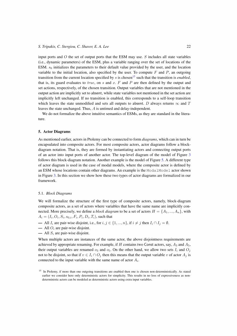
S. Tripakis, C. Stergiou, C. Shaver, E. A. Lee 22

input ports and O the set of output ports that the ESM may use. S includes all state variables(i.e., dynamic parameters) of the ESM, plus a variable ranging over the set of locations of theESM. s0 initializes the parameters to their default value provided by the user, and the locationvariable to the initial location, also specified by the user. To compute F and P , an outgoingtransition from the current location specified by s is chosen15 such that the transition is enabled,that is, its guard evaluates to true , on s and x. F and P are then defined by the output andset actions, respectively, of the chosen transition. Output variables that are not mentioned in theoutput action are implicitly set to absent, while state variables not mentioned in the set action areimplicitly left unchanged. If no transition is enabled, this corresponds to a self-loop transitionwhich leaves the state unmodified and sets all outputs to absent. D always returns ∞ and Tleaves the state unchanged. Thus, A is untimed and delay-independent.

We do not formalize the above intuitive semantics of ESMs, as they are standard in the litera-ture.

5. Actor Diagrams

As mentioned earlier, actors in Ptolemy can be connected to form diagrams, which can in turn beencapsulated into composite actors. For most composite actors, actor diagrams follow a block-diagram notation. That is, they are formed by instantiating actors and connecting output portsof an actor into input ports of another actor. The top-level diagram of the model of Figure 3follows this block-diagram notation. Another example is the model of Figure 5. A different typeof actor diagram is used in the case of modal models, where the composite actor is defined byan ESM whose locations contain other diagrams. An example is the ModalModel actor shownin Figure 3. In this section we show how these two types of actor diagrams are formalized in ourframework.

5.1. Block Diagrams

We will formalize the structure of the first type of composite actors, namely, block-diagramcomposite actors, as a set of actors where variables that have the same name are implicitly con-nected. More precisely, we define a block diagram to be a set of actors H = {A1, ..., An}, withAi = (Ii, Oi, Si, s0,i, Fi, Pi, Di, Ti), such that

— All Ii are pair-wise disjoint, i.e., for i, j ∈ {1, ..., n}, if i 6= j then Ii ∩ Ij = ∅.— All Oi are pair-wise disjoint.— All Si are pair-wise disjoint.

When multiple actors are instances of the same actor, the above disjointness requirements areachieved by appropriate renaming. For example, ifH contains two Const actors, say,A3 andA5,their output variables are renamed o3 and o5. On the other hand, we allow two sets Ii and Ojnot to be disjoint, so that if v ∈ Ii ∩Oj then this means that the output variable v of actor Aj isconnected to the input variable with the same name of actor Ai.

15 In Ptolemy, if more than one outgoing transitions are enabled then one is chosen non-deterministically. As statedearlier we consider here only deterministic actors for simplicity. This results in no loss of expressiveness as non-deterministic actors can be modeled as deterministic actors using extra input variables.

A Modular Formal Semantics for Ptolemy 23

Fan-out, where an output variable o of some actor is connected to the input variables v1, v2, ...

of multiple actors, is modeled by adding an explicit actor Fanout with input o and outputsv1, v2, .... Fanout is a stateless actor that “copies” its input to all its outputs every time it fires.

Feedback loops can be formed by connecting an output variable of an actor to one of its inputvariables. However, since in order to avoid confusion we assume that input and output variablesare disjoint, we model feedback by including an additional Id actor in the connection.

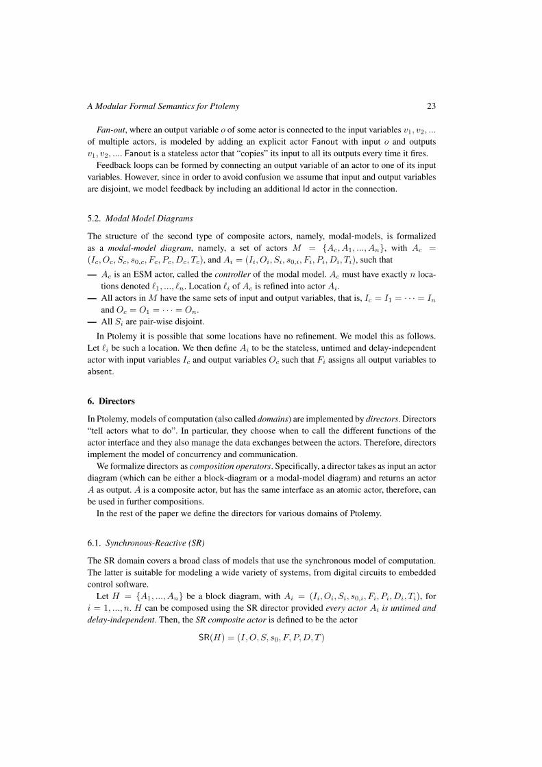
5.2. Modal Model Diagrams

The structure of the second type of composite actors, namely, modal-models, is formalizedas a modal-model diagram, namely, a set of actors M = {Ac, A1, ..., An}, with Ac =

(Ic, Oc, Sc, s0,c, Fc, Pc, Dc, Tc), and Ai = (Ii, Oi, Si, s0,i, Fi, Pi, Di, Ti), such that

— Ac is an ESM actor, called the controller of the modal model. Ac must have exactly n loca-tions denoted `1, ..., `n. Location `i of Ac is refined into actor Ai.

— All actors in M have the same sets of input and output variables, that is, Ic = I1 = · · · = Inand Oc = O1 = · · · = On.

— All Si are pair-wise disjoint.

In Ptolemy it is possible that some locations have no refinement. We model this as follows.Let `i be such a location. We then define Ai to be the stateless, untimed and delay-independentactor with input variables Ic and output variables Oc such that Fi assigns all output variables toabsent.

6. Directors

In Ptolemy, models of computation (also called domains) are implemented by directors. Directors“tell actors what to do”. In particular, they choose when to call the different functions of theactor interface and they also manage the data exchanges between the actors. Therefore, directorsimplement the model of concurrency and communication.

We formalize directors as composition operators. Specifically, a director takes as input an actordiagram (which can be either a block-diagram or a modal-model diagram) and returns an actorA as output. A is a composite actor, but has the same interface as an atomic actor, therefore, canbe used in further compositions.

In the rest of the paper we define the directors for various domains of Ptolemy.

6.1. Synchronous-Reactive (SR)

The SR domain covers a broad class of models that use the synchronous model of computation.The latter is suitable for modeling a wide variety of systems, from digital circuits to embeddedcontrol software.

Let H = {A1, ..., An} be a block diagram, with Ai = (Ii, Oi, Si, s0,i, Fi, Pi, Di, Ti), fori = 1, ..., n. H can be composed using the SR director provided every actor Ai is untimed anddelay-independent. Then, the SR composite actor is defined to be the actor

SR(H) = (I,O, S, s0, F, P,D, T )

S. Tripakis, C. Stergiou, C. Shaver, E. A. Lee 24

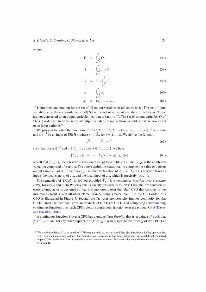
where:

V =

n⋃i=1

Oi (57)

I =

n⋃i=1

Ii \ V (58)

O = V \n⋃i=1

Ii (59)

S =

n⋃i=1

Si (60)

s0 = (s0,1, ..., s0,n) (61)

V is intermediate notation for the set of all output variables of all actors in H . The set of inputvariables I of the composite actor SR(H) is the set of all input variables of actors in H thatare not connected to an output variable, i.e., that are not in V . The set of output variables O ofSR(H) is defined to be the set of all output variables V minus those variables that are connectedto an input variable.16

We proceed to define the functions F, P,D, T of SR(H). Let s = (s1, ..., sn) ∈ S be a stateand x ∈ I be an input of SR(H), where si ∈ Si, for i = 1, ..., n. We define the function

Fs,x : V → V (62)

such that, for y ∈ V and o ∈ Oj , for some j ∈ {1, ..., n}, we have(Fs,x(y)

)(o) = Fj

(sj , (x, y) �Ij

)(o) (63)

Recall that (x, y) �Ij denotes the restriction of (x, y) to variables in Ij and (x, y) is the combinedvaluation composed of x and y. The above definition states that, to compute the value of a givenoutput variable o of Aj , function Fs,x uses the fire function of Aj , i.e., Fj . This function takes asinputs the local state sj of Aj , and the local input of Aj , which is precisely (x, y) �Ij .

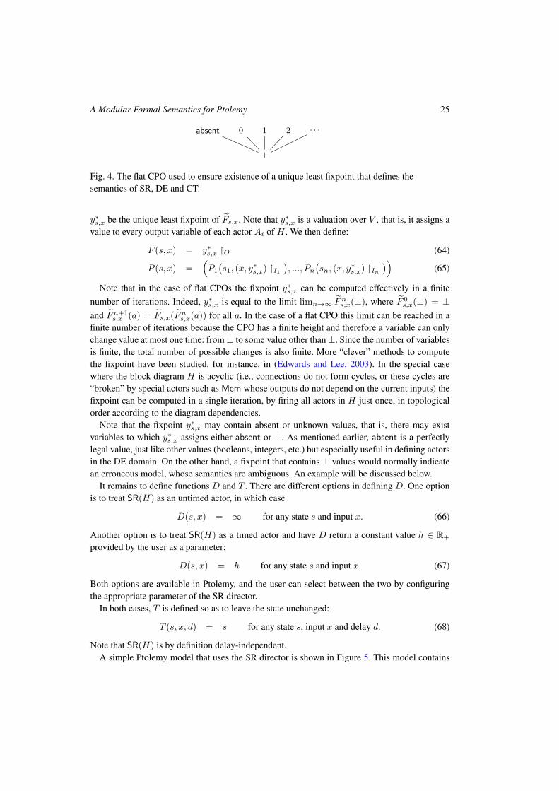
The semantics of SR(H) is defined provided Fs,x is a continuous function over a certainCPO, for any s and x. In Ptolemy this is usually ensured as follows: First, the fire function ofevery atomic actor is designed so that it is monotonic over the “flat” CPO that consists of theminimal element ⊥ and all other elements in U being greater than ⊥ in the CPO order: thisCPO is illustrated in Figure 4. Second, the fact that monotonicity implies continuity for flatCPOs. Third, the fact that Cartesian products of CPOs are CPOs, and composing correspondingcontinuous functions over such CPOs yields a continuous function over the product CPO (Daveyand Priestley, 2002).

A continuous function f over a CPO has a unique least fixpoint, that is, a unique x∗ such thatf(x∗) = x∗ and for any other fixpoint x of f , x∗ ≤ x with respect to the order≤ of the CPO. Let

16 We could also define O to be equal to V . We opt not to do so, as we should then also introduce a hiding operator thatremoves some unnecessary outputs. The definition we use results in this hiding happening by default to all connectedoutputs. This results in no loss of generality, as we can always add explicit actors that copy the outputs that we do notwish to hide.

A Modular Formal Semantics for Ptolemy 25

⊥

1 2 · · ·0absent

Fig. 4. The flat CPO used to ensure existence of a unique least fixpoint that defines thesemantics of SR, DE and CT.

y∗s,x be the unique least fixpoint of Fs,x. Note that y∗s,x is a valuation over V , that is, it assigns avalue to every output variable of each actor Ai of H . We then define:

F (s, x) = y∗s,x �O (64)

P (s, x) =(P1

(s1, (x, y

∗s,x) �I1

), ..., Pn

(sn, (x, y

∗s,x) �In

))(65)

Note that in the case of flat CPOs the fixpoint y∗s,x can be computed effectively in a finitenumber of iterations. Indeed, y∗s,x is equal to the limit limn→∞ Fns,x(⊥), where F 0

s,x(⊥) = ⊥and Fn+1

s,x (a) = Fs,x(Fns,x(a)) for all a. In the case of a flat CPO this limit can be reached in afinite number of iterations because the CPO has a finite height and therefore a variable can onlychange value at most one time: from⊥ to some value other than⊥. Since the number of variablesis finite, the total number of possible changes is also finite. More “clever” methods to computethe fixpoint have been studied, for instance, in (Edwards and Lee, 2003). In the special casewhere the block diagram H is acyclic (i.e., connections do not form cycles, or these cycles are“broken” by special actors such as Mem whose outputs do not depend on the current inputs) thefixpoint can be computed in a single iteration, by firing all actors in H just once, in topologicalorder according to the diagram dependencies.

Note that the fixpoint y∗s,x may contain absent or unknown values, that is, there may existvariables to which y∗s,x assigns either absent or ⊥. As mentioned earlier, absent is a perfectlylegal value, just like other values (booleans, integers, etc.) but especially useful in defining actorsin the DE domain. On the other hand, a fixpoint that contains ⊥ values would normally indicatean erroneous model, whose semantics are ambiguous. An example will be discussed below.

It remains to define functions D and T . There are different options in defining D. One optionis to treat SR(H) as an untimed actor, in which case

D(s, x) = ∞ for any state s and input x. (66)

Another option is to treat SR(H) as a timed actor and have D return a constant value h ∈ R+

provided by the user as a parameter:

D(s, x) = h for any state s and input x. (67)

Both options are available in Ptolemy, and the user can select between the two by configuringthe appropriate parameter of the SR director.

In both cases, T is defined so as to leave the state unchanged:

T (s, x, d) = s for any state s, input x and delay d. (68)

Note that SR(H) is by definition delay-independent.A simple Ptolemy model that uses the SR director is shown in Figure 5. This model contains

S. Tripakis, C. Stergiou, C. Shaver, E. A. Lee 26

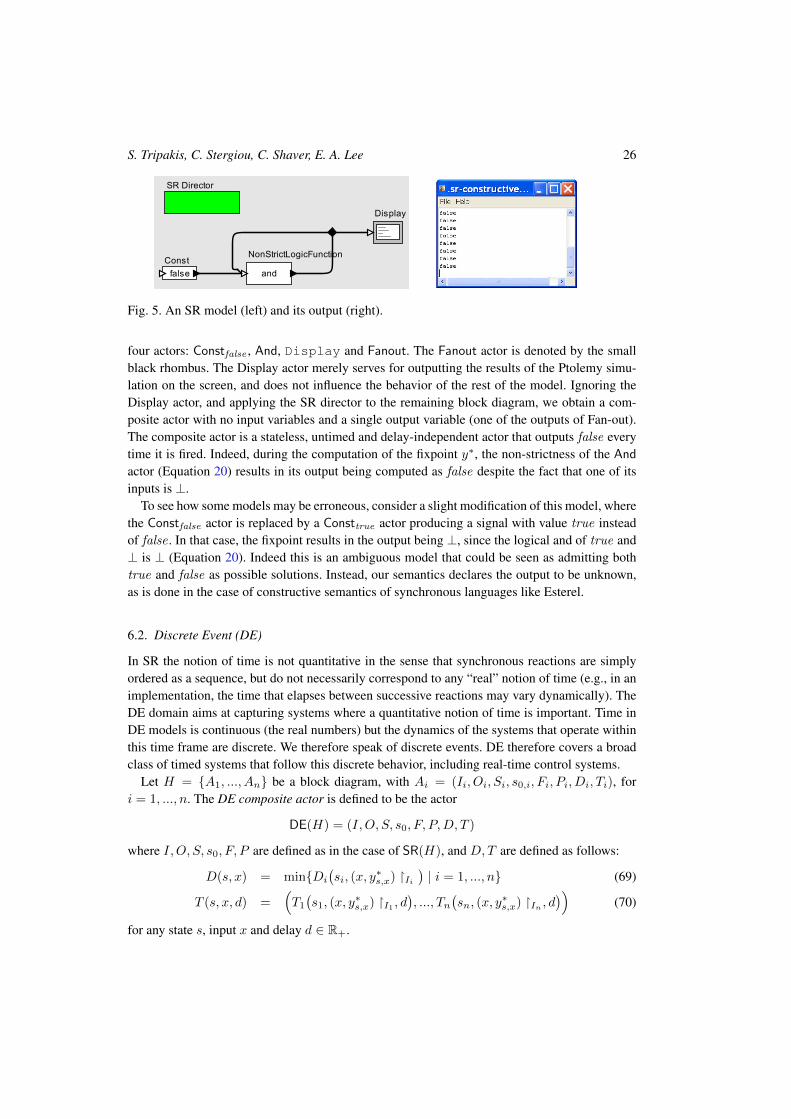
Fig. 5. An SR model (left) and its output (right).

four actors: Constfalse , And, Display and Fanout. The Fanout actor is denoted by the smallblack rhombus. The Display actor merely serves for outputting the results of the Ptolemy simu-lation on the screen, and does not influence the behavior of the rest of the model. Ignoring theDisplay actor, and applying the SR director to the remaining block diagram, we obtain a com-posite actor with no input variables and a single output variable (one of the outputs of Fan-out).The composite actor is a stateless, untimed and delay-independent actor that outputs false everytime it is fired. Indeed, during the computation of the fixpoint y∗, the non-strictness of the And

actor (Equation 20) results in its output being computed as false despite the fact that one of itsinputs is ⊥.

To see how some models may be erroneous, consider a slight modification of this model, wherethe Constfalse actor is replaced by a Consttrue actor producing a signal with value true insteadof false . In that case, the fixpoint results in the output being ⊥, since the logical and of true and⊥ is ⊥ (Equation 20). Indeed this is an ambiguous model that could be seen as admitting bothtrue and false as possible solutions. Instead, our semantics declares the output to be unknown,as is done in the case of constructive semantics of synchronous languages like Esterel.

6.2. Discrete Event (DE)

In SR the notion of time is not quantitative in the sense that synchronous reactions are simplyordered as a sequence, but do not necessarily correspond to any “real” notion of time (e.g., in animplementation, the time that elapses between successive reactions may vary dynamically). TheDE domain aims at capturing systems where a quantitative notion of time is important. Time inDE models is continuous (the real numbers) but the dynamics of the systems that operate withinthis time frame are discrete. We therefore speak of discrete events. DE therefore covers a broadclass of timed systems that follow this discrete behavior, including real-time control systems.

Let H = {A1, ..., An} be a block diagram, with Ai = (Ii, Oi, Si, s0,i, Fi, Pi, Di, Ti), fori = 1, ..., n. The DE composite actor is defined to be the actor

DE(H) = (I,O, S, s0, F, P,D, T )

where I,O, S, s0, F, P are defined as in the case of SR(H), and D,T are defined as follows:

D(s, x) = min{Di

(si, (x, y

∗s,x) �Ii

)| i = 1, ..., n} (69)

T (s, x, d) =(T1

(s1, (x, y

∗s,x) �I1 , d

), ..., Tn

(sn, (x, y

∗s,x) �In , d

))(70)

for any state s, input x and delay d ∈ R+.

A Modular Formal Semantics for Ptolemy 27

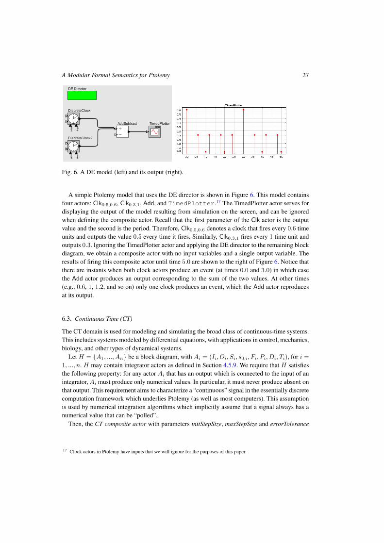
Fig. 6. A DE model (left) and its output (right).

A simple Ptolemy model that uses the DE director is shown in Figure 6. This model containsfour actors: Clk0.5,0.6, Clk0.3,1, Add, and TimedPlotter.17 The TimedPlotter actor serves fordisplaying the output of the model resulting from simulation on the screen, and can be ignoredwhen defining the composite actor. Recall that the first parameter of the Clk actor is the outputvalue and the second is the period. Therefore, Clk0.5,0.6 denotes a clock that fires every 0.6 timeunits and outputs the value 0.5 every time it fires. Similarly, Clk0.3,1 fires every 1 time unit andoutputs 0.3. Ignoring the TimedPlotter actor and applying the DE director to the remaining blockdiagram, we obtain a composite actor with no input variables and a single output variable. Theresults of firing this composite actor until time 5.0 are shown to the right of Figure 6. Notice thatthere are instants when both clock actors produce an event (at times 0.0 and 3.0) in which casethe Add actor produces an output corresponding to the sum of the two values. At other times(e.g., 0.6, 1, 1.2, and so on) only one clock produces an event, which the Add actor reproducesat its output.

6.3. Continuous Time (CT)

The CT domain is used for modeling and simulating the broad class of continuous-time systems.This includes systems modeled by differential equations, with applications in control, mechanics,biology, and other types of dynamical systems.

Let H = {A1, ..., An} be a block diagram, with Ai = (Ii, Oi, Si, s0,i, Fi, Pi, Di, Ti), for i =

1, ..., n. H may contain integrator actors as defined in Section 4.5.9. We require that H satisfiesthe following property: for any actor Ai that has an output which is connected to the input of anintegrator,Ai must produce only numerical values. In particular, it must never produce absent onthat output. This requirement aims to characterize a “continuous” signal in the essentially discretecomputation framework which underlies Ptolemy (as well as most computers). This assumptionis used by numerical integration algorithms which implicitly assume that a signal always has anumerical value that can be “polled”.

Then, the CT composite actor with parameters initStepSize, maxStepSize and errorTolerance

17 Clock actors in Ptolemy have inputs that we will ignore for the purposes of this paper.

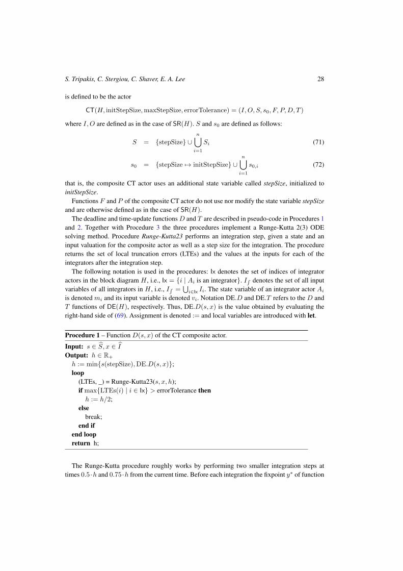
S. Tripakis, C. Stergiou, C. Shaver, E. A. Lee 28

is defined to be the actor

CT(H, initStepSize,maxStepSize, errorTolerance) = (I,O, S, s0, F, P,D, T )

where I,O are defined as in the case of SR(H). S and s0 are defined as follows:

S = {stepSize} ∪n⋃i=1

Si (71)

s0 = {stepSize 7→ initStepSize} ∪n⋃i=1

s0,i (72)

that is, the composite CT actor uses an additional state variable called stepSize, initialized toinitStepSize.

Functions F and P of the composite CT actor do not use nor modify the state variable stepSizeand are otherwise defined as in the case of SR(H).

The deadline and time-update functionsD and T are described in pseudo-code in Procedures 1and 2. Together with Procedure 3 the three procedures implement a Runge-Kutta 2(3) ODEsolving method. Procedure Runge-Kutta23 performs an integration step, given a state and aninput valuation for the composite actor as well as a step size for the integration. The procedurereturns the set of local truncation errors (LTEs) and the values at the inputs for each of theintegrators after the integration step.

The following notation is used in the procedures: Ix denotes the set of indices of integratoractors in the block diagram H , i.e., Ix = {i | Ai is an integrator}. I∫ denotes the set of all inputvariables of all integrators in H , i.e., I∫ =

⋃i∈Ix Ii. The state variable of an integrator actor Ai

is denoted mi and its input variable is denoted vi. Notation DE.D and DE.T refers to the D andT functions of DE(H), respectively. Thus, DE.D(s, x) is the value obtained by evaluating theright-hand side of (69). Assignment is denoted := and local variables are introduced with let.

Procedure 1 – Function D(s, x) of the CT composite actor.

Input: s ∈ S, x ∈ IOutput: h ∈ R+

h := min{s(stepSize),DE.D(s, x)};loop

(LTEs, _) = Runge-Kutta23(s, x, h);if max{LTEs(i) | i ∈ Ix} > errorTolerance thenh := h/2;

elsebreak;

end ifend loopreturn h;

The Runge-Kutta procedure roughly works by performing two smaller integration steps attimes 0.5 ·h and 0.75 ·h from the current time. Before each integration the fixpoint y∗ of function

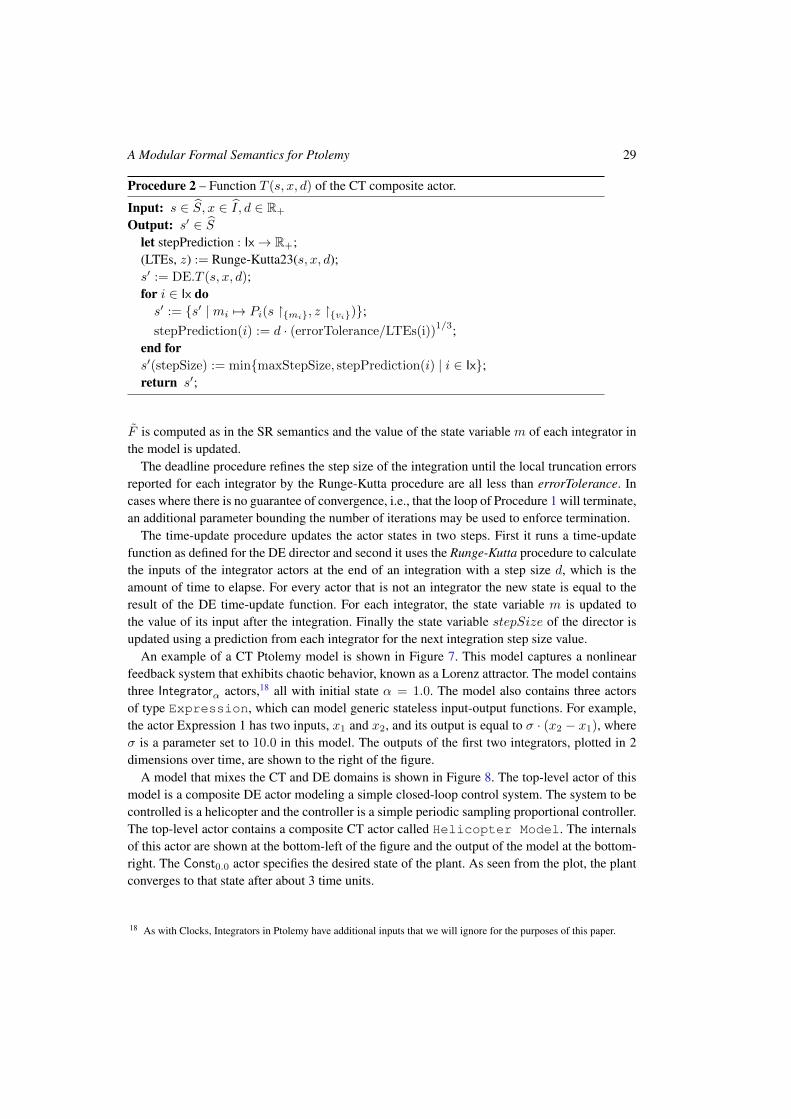
A Modular Formal Semantics for Ptolemy 29

Procedure 2 – Function T (s, x, d) of the CT composite actor.

Input: s ∈ S, x ∈ I , d ∈ R+

Output: s′ ∈ Slet stepPrediction : Ix→ R+;(LTEs, z) := Runge-Kutta23(s, x, d);s′ := DE.T (s, x, d);for i ∈ Ix dos′ := {s′ | mi 7→ Pi(s �{mi}, z �{vi})};stepPrediction(i) := d · (errorTolerance/LTEs(i))

1/3;end fors′(stepSize) := min{maxStepSize, stepPrediction(i) | i ∈ Ix};return s′;

F is computed as in the SR semantics and the value of the state variable m of each integrator inthe model is updated.

The deadline procedure refines the step size of the integration until the local truncation errorsreported for each integrator by the Runge-Kutta procedure are all less than errorTolerance. Incases where there is no guarantee of convergence, i.e., that the loop of Procedure 1 will terminate,an additional parameter bounding the number of iterations may be used to enforce termination.

The time-update procedure updates the actor states in two steps. First it runs a time-updatefunction as defined for the DE director and second it uses the Runge-Kutta procedure to calculatethe inputs of the integrator actors at the end of an integration with a step size d, which is theamount of time to elapse. For every actor that is not an integrator the new state is equal to theresult of the DE time-update function. For each integrator, the state variable m is updated tothe value of its input after the integration. Finally the state variable stepSize of the director isupdated using a prediction from each integrator for the next integration step size value.

An example of a CT Ptolemy model is shown in Figure 7. This model captures a nonlinearfeedback system that exhibits chaotic behavior, known as a Lorenz attractor. The model containsthree Integratorα actors,18 all with initial state α = 1.0. The model also contains three actorsof type Expression, which can model generic stateless input-output functions. For example,the actor Expression 1 has two inputs, x1 and x2, and its output is equal to σ · (x2 − x1), whereσ is a parameter set to 10.0 in this model. The outputs of the first two integrators, plotted in 2dimensions over time, are shown to the right of the figure.

A model that mixes the CT and DE domains is shown in Figure 8. The top-level actor of thismodel is a composite DE actor modeling a simple closed-loop control system. The system to becontrolled is a helicopter and the controller is a simple periodic sampling proportional controller.The top-level actor contains a composite CT actor called Helicopter Model. The internalsof this actor are shown at the bottom-left of the figure and the output of the model at the bottom-right. The Const0.0 actor specifies the desired state of the plant. As seen from the plot, the plantconverges to that state after about 3 time units.

18 As with Clocks, Integrators in Ptolemy have additional inputs that we will ignore for the purposes of this paper.

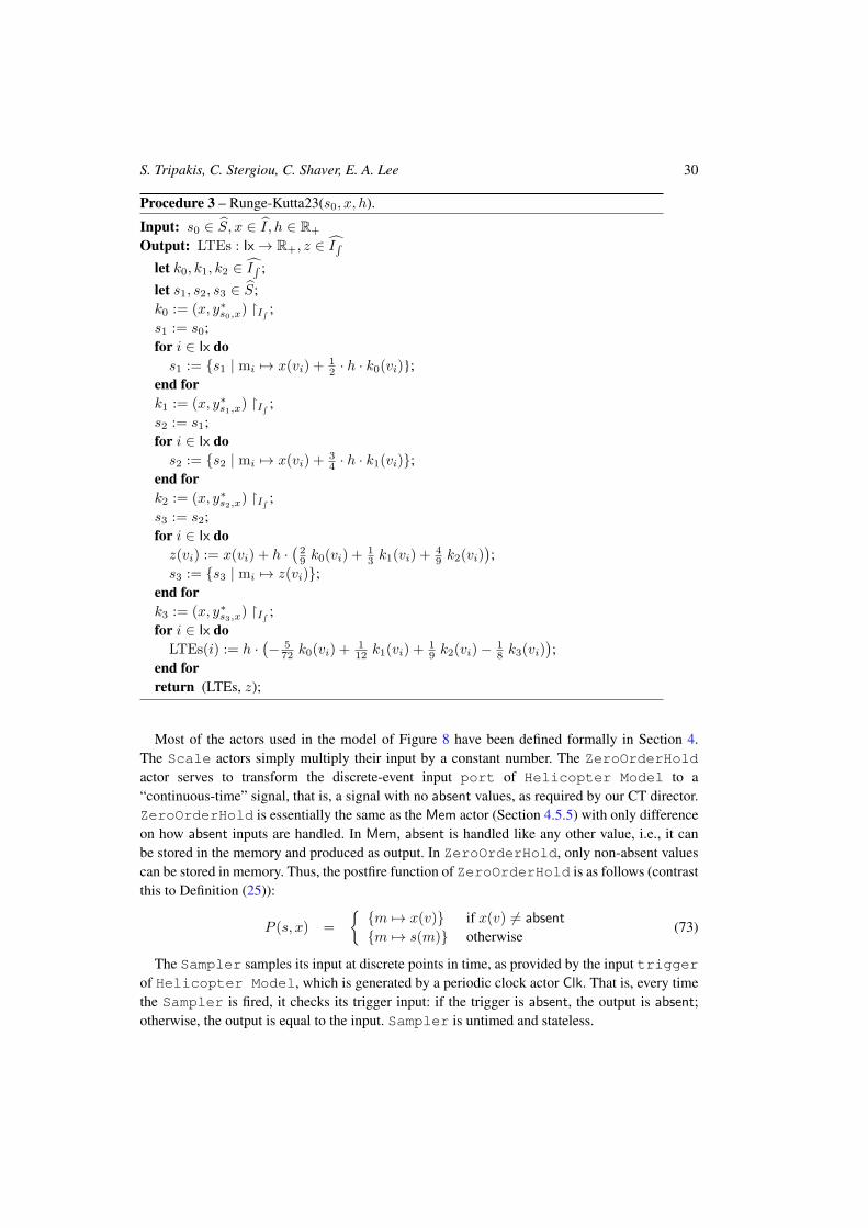
S. Tripakis, C. Stergiou, C. Shaver, E. A. Lee 30

Procedure 3 – Runge-Kutta23(s0, x, h).

Input: s0 ∈ S, x ∈ I , h ∈ R+

Output: LTEs : Ix→ R+, z ∈ I∫let k0, k1, k2 ∈ I∫ ;

let s1, s2, s3 ∈ S;k0 := (x, y∗s0,x) �I∫ ;s1 := s0;for i ∈ Ix dos1 := {s1 | mi 7→ x(vi) + 1

2 · h · k0(vi)};end fork1 := (x, y∗s1,x) �I∫ ;s2 := s1;for i ∈ Ix dos2 := {s2 | mi 7→ x(vi) + 3

4 · h · k1(vi)};end fork2 := (x, y∗s2,x) �I∫ ;s3 := s2;for i ∈ Ix doz(vi) := x(vi) + h ·

(29 k0(vi) + 1

3 k1(vi) + 49 k2(vi)

);

s3 := {s3 | mi 7→ z(vi)};end fork3 := (x, y∗s3,x) �I∫ ;for i ∈ Ix do

LTEs(i) := h ·(− 5

72 k0(vi) + 112 k1(vi) + 1

9 k2(vi)− 18 k3(vi)

);

end forreturn (LTEs, z);

Most of the actors used in the model of Figure 8 have been defined formally in Section 4.The Scale actors simply multiply their input by a constant number. The ZeroOrderHoldactor serves to transform the discrete-event input port of Helicopter Model to a“continuous-time” signal, that is, a signal with no absent values, as required by our CT director.ZeroOrderHold is essentially the same as the Mem actor (Section 4.5.5) with only differenceon how absent inputs are handled. In Mem, absent is handled like any other value, i.e., it canbe stored in the memory and produced as output. In ZeroOrderHold, only non-absent valuescan be stored in memory. Thus, the postfire function of ZeroOrderHold is as follows (contrastthis to Definition (25)):

P (s, x) =

{{m 7→ x(v)} if x(v) 6= absent

{m 7→ s(m)} otherwise(73)

The Sampler samples its input at discrete points in time, as provided by the input triggerof Helicopter Model, which is generated by a periodic clock actor Clk. That is, every timethe Sampler is fired, it checks its trigger input: if the trigger is absent, the output is absent;otherwise, the output is equal to the input. Sampler is untimed and stateless.

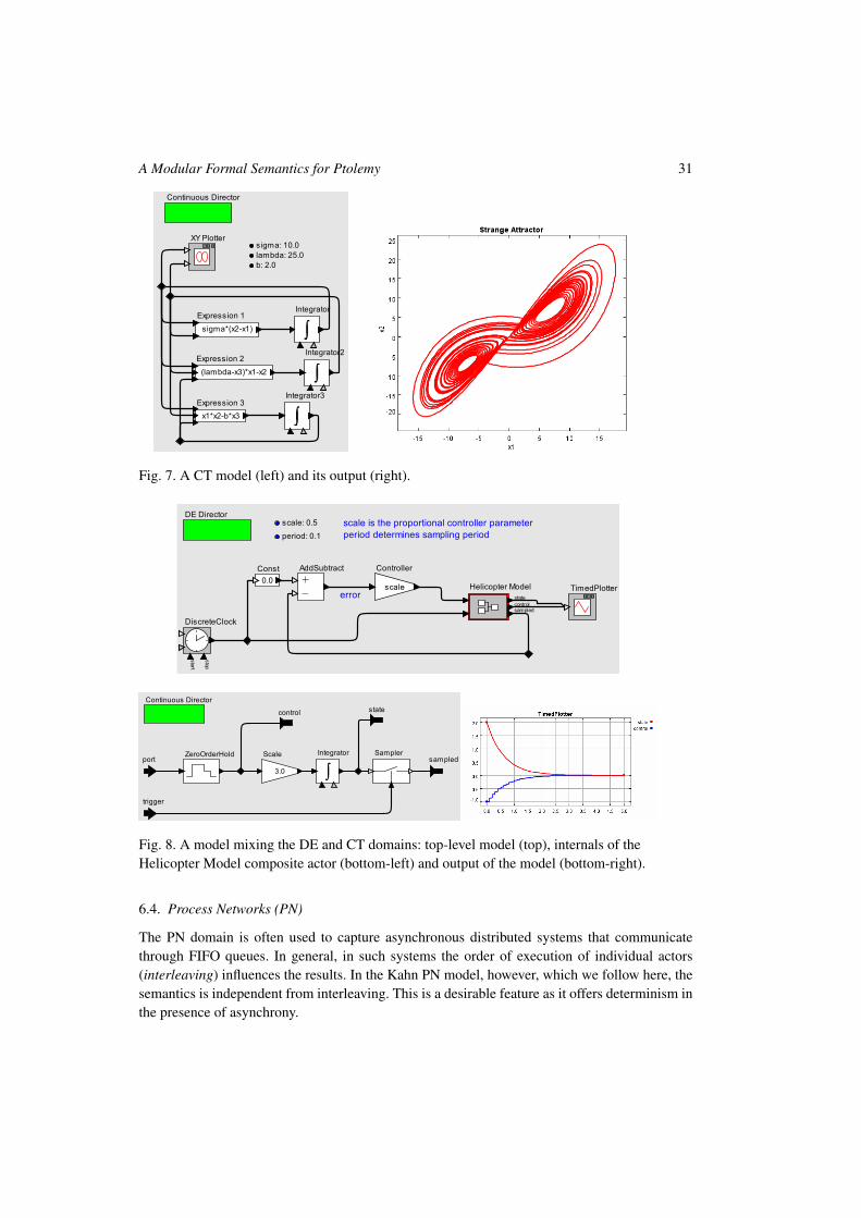
A Modular Formal Semantics for Ptolemy 31

Fig. 7. A CT model (left) and its output (right).

Fig. 8. A model mixing the DE and CT domains: top-level model (top), internals of theHelicopter Model composite actor (bottom-left) and output of the model (bottom-right).

6.4. Process Networks (PN)

The PN domain is often used to capture asynchronous distributed systems that communicatethrough FIFO queues. In general, in such systems the order of execution of individual actors(interleaving) influences the results. In the Kahn PN model, however, which we follow here, thesemantics is independent from interleaving. This is a desirable feature as it offers determinism inthe presence of asynchrony.

S. Tripakis, C. Stergiou, C. Shaver, E. A. Lee 32

Let H = {A1, ..., An} be a block diagram, with Ai = (Ii, Oi, Si, s0,i, Fi, Pi, Di, Ti), fori = 1, ..., n. H can be composed using the PN director provided every actor Ai is a dataflow,untimed and delay-independent actor. The fact that Ai is dataflow means that variables in Ii andOi range over streams. Then, the PN composite actor is defined to be the actor

PN(H) = (I,O, S, s0, F, P,D, T )

where I,O, S, s0 are defined as in the case of SR(H).The semantics for PN follows the semantics of Kahn Process Networks (Kahn, 1974). Specifi-

cally, F is defined using a fixpoint semantics similarly to the SR case, but with a major difference:in the SR case the CPO is the flat CPO shown in Figure 4, whereas in the PN case the CPO is theset of all (finite or infinite) streams ordered with the prefix order. Stream ρ is a prefix of stream ρ′

iff there exists stream ρ′′ such that ρ′ = ρ · ρ′′, where · denotes stream concatenation. Notice thatρ′ = ρ · ρ′′ implies that either ρ is finite, or it is infinite in which case ρ′ = ρ and ρ′′ = []. Theleast element in the CPO of streams is the empty stream [] (i.e., the sequence of length 0). Actorsare required to be monotonic (in fact, continuous) in this CPO, essentially meaning that longerinput streams can only result in longer output streams. Then, the definitions of F and P for PNcan be given by the same Equations (62)–(65) used for SR, and will therefore not be repeatedhere. This definition ensures that continuity is preserved, that is, if all actors Ai are continuousthen so is the resulting composite actor PN(H).

The definition of D for PN can also follow the definition for SR. PN is essentially an un-timed model of computation, but, like SR, could be given timed semantics for convenience ofembedding it into timed models. The definition of T for PN is also as in SR: PN(H) is a delay-independent actor, like its sub-actors.

A simple Ptolemy model that uses the PN director is shown in Figure 9. This model containsfive actors: Ramp, AddSubtract, SampleDelay, Display and Fanout. Ramp producesthe infinite stream [1, 2, · · · ]. SampleDelay produces as output the stream it receives as inputprefixed by the element 0. For example, if it receives [1, 2] it produces [0, 1, 2]. AddSubtractis the extension of Add to streams: it adds streams in an element-wise fashion, up to the lengthof the shorter input stream.19

6.5. Modal Models (MM)

Modal models are hierarchical models where the top level model consists of an ESM, the statesof which are refined into other models (possibly from different domains). Modal models aresuitable for a number of applications. They are especially useful in describing event-driven andmodal behavior, where the system’s operation changes dynamically by switching among a finiteset of modes. Such changes may be triggered by user inputs, sensor data, hardware failures, orother types of events, and are essential in fault management, adaptivity, and reconfigurability

19 In Ptolemy, many actors are polymorphic in the sense that they can operate under different directors and with differenttypes of inputs and outputs. AddSubtract is such an actor: it can add scalars of numerical type (integers, reals, etc.)as well as streams. We do not provide a formal treatment of actor polymorphism, as this would involve a more or lesscomplete type theory for actors, which is beyond the scope of this paper.

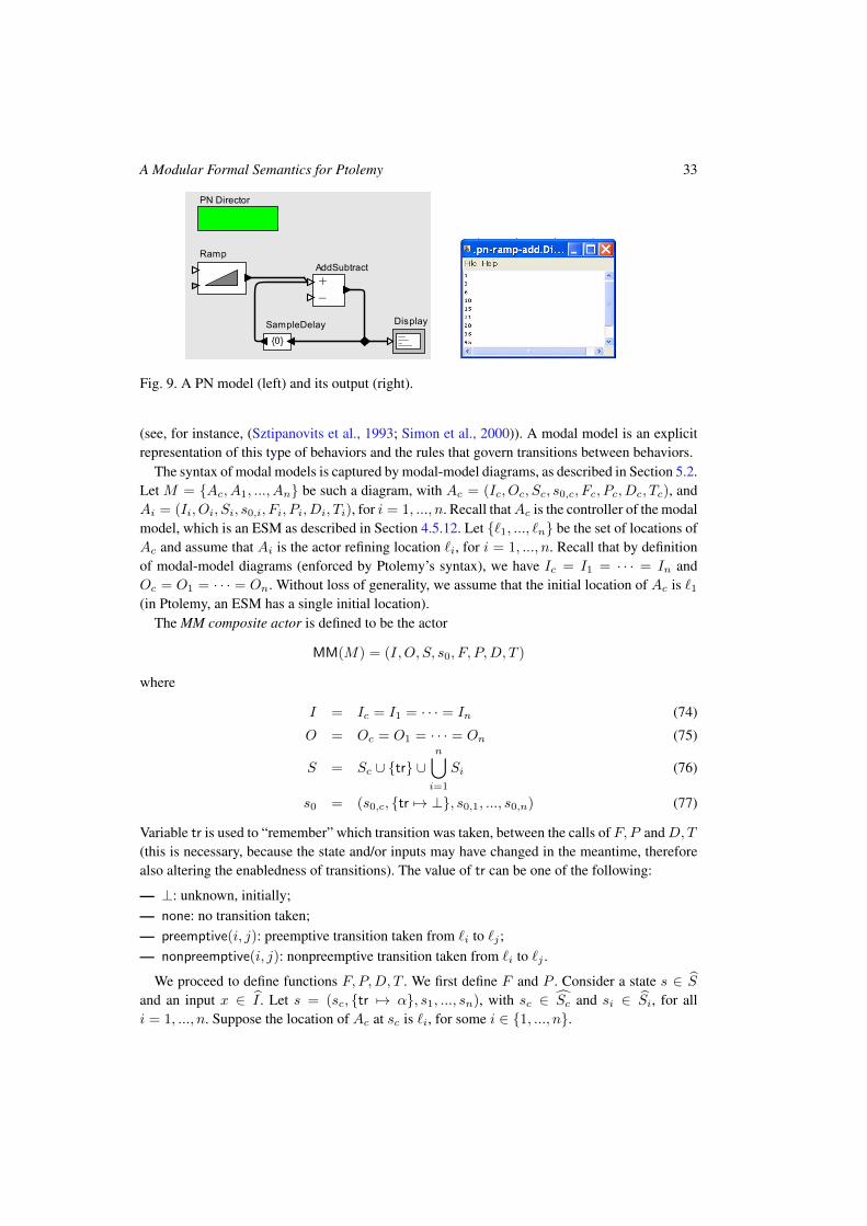
A Modular Formal Semantics for Ptolemy 33

Fig. 9. A PN model (left) and its output (right).

(see, for instance, (Sztipanovits et al., 1993; Simon et al., 2000)). A modal model is an explicitrepresentation of this type of behaviors and the rules that govern transitions between behaviors.

The syntax of modal models is captured by modal-model diagrams, as described in Section 5.2.Let M = {Ac, A1, ..., An} be such a diagram, with Ac = (Ic, Oc, Sc, s0,c, Fc, Pc, Dc, Tc), andAi = (Ii, Oi, Si, s0,i, Fi, Pi, Di, Ti), for i = 1, ..., n. Recall thatAc is the controller of the modalmodel, which is an ESM as described in Section 4.5.12. Let {`1, ..., `n} be the set of locations ofAc and assume that Ai is the actor refining location `i, for i = 1, ..., n. Recall that by definitionof modal-model diagrams (enforced by Ptolemy’s syntax), we have Ic = I1 = · · · = In andOc = O1 = · · · = On. Without loss of generality, we assume that the initial location of Ac is `1(in Ptolemy, an ESM has a single initial location).

The MM composite actor is defined to be the actor

MM(M) = (I,O, S, s0, F, P,D, T )

where

I = Ic = I1 = · · · = In (74)

O = Oc = O1 = · · · = On (75)

S = Sc ∪ {tr} ∪n⋃i=1

Si (76)

s0 = (s0,c, {tr 7→ ⊥}, s0,1, ..., s0,n) (77)

Variable tr is used to “remember” which transition was taken, between the calls of F, P andD,T(this is necessary, because the state and/or inputs may have changed in the meantime, thereforealso altering the enabledness of transitions). The value of tr can be one of the following:

— ⊥: unknown, initially;— none: no transition taken;— preemptive(i, j): preemptive transition taken from `i to `j ;— nonpreemptive(i, j): nonpreemptive transition taken from `i to `j .

We proceed to define functions F, P,D, T . We first define F and P . Consider a state s ∈ Sand an input x ∈ I . Let s = (sc, {tr 7→ α}, s1, ..., sn), with sc ∈ Sc and si ∈ Si, for alli = 1, ..., n. Suppose the location of Ac at sc is `i, for some i ∈ {1, ..., n}.

S. Tripakis, C. Stergiou, C. Shaver, E. A. Lee 34

6.5.1. Strict modal models: We will first present a strict interpretation of the semantics of modalmodels, where we can assume that the enabledness status of all outgoing transitions from `i(that is, whether the guard of each transition evaluates to true or false) can be determined. Theenabledness of a transition may not be known due to some inputs being unknown (i.e., ⊥). E.g.,if x is an input variable and x = ⊥, then the guard x ≥ 0 evaluates to neither true nor false , butto ⊥. Figure 10 shows an example, which will be discussed later.

In the strict interpretation, if guards are unknown then all outputs can be also set to be ⊥. InSection 6.5.2 we provide a non-strict interpretation where outputs can be assigned to values otherthan unknown, even if some inputs are unknown. This is inspired by non-strict but constructivesemantics, such as those we presented for SR, or those used in Esterel.

For the strict interpretation, we distinguish the following cases:

1 There are no outgoing transitions of Ac from location li that are enabled at s and x. Then:

F (s, x) = Fi(si, x) (78)

P (s, x) = (sc, {tr 7→ none}, s1, ..., si−1, Pi(si, x), si+1, ..., sn) (79)

2 There exists a preemptive outgoing transition from `i to `j that is enabled at s and x. Denotethe output action and set action of this transition by β and γ, respectively. Then:

F (s, x) = β(s, x) (80)

P (s, x) = (s′c, {tr 7→ preemptive(i, j)}, s1, ..., sj−1, s′j , sj+1, ..., sn) (81)

where:

(a) β(s, x) denotes the output obtained by applying the output action β to s and x,(b) s′c is obtained by applying the set action γ to s and x and setting the location of Ac to `j ,(c) s′j is obtained by applying the set action γ to s and x.

3 There are no preemptive outgoing transitions from `i that are enabled at s and x, but thereexists a non-preemptive outgoing transition from `i to `j that is enabled at s and x. Denotethe output action and set action of this transition by β and γ, respectively. Then:

F (s, x) = β(s, x, Fi(s, x)) (82)

P (s, x) = (s′c, {tr 7→ nonpreemptive(i, j)}, s1, ..., s′i, ..., s

′j , ..., sn) (83)

where:

(a) β(s, x, Fi(s, x)) denotes the output obtained by first computing the output y = Fi(s, x)

and then applying the output action β to y, s and x,(b) s′c is obtained as in Case 2b,(c) s′j is obtained as in Case 2c,(d) s′i is obtained by first computing s′′i = Pi(si, x) and then applying the set action γ to s′′i ,

Item 1 treats the case where no transition of the controller is enabled: in this case, the locationof the controller remains unchanged and the modal model M behaves (i.e., fires and postfires)like its current refinement Mi.

Item 2 treats the case where preemptive transitions of the controller are enabled (possibly inaddition to non-preemptive transitions). In this case the preemptive transitions preempt the firingand postfiring of Mi, and the outputs and state updates are produced solely by the output and

A Modular Formal Semantics for Ptolemy 35

set actions of the transition. We will not define formally the effect of those actions, as they arestandard. Note that the set action γ may reset some state variables of the target refinement Ajto their initial values. This is done in particular if the transition is a reset transition. Also, γ may“copy” the value of some other state variable, possibly of another refinement, to a state variableof the target refinement. In particular, when modeling hybrid systems (Manna and Pnueli, 1992),the state variables in all refinements are typically the same, i.e., copies of each other. In that case,when moving from one mode of operation to the next, the state of the system must be preserved.This can be done with the appropriate set actions.

Item 3 treats the case where only non-preemptive transitions of the controller are enabled. Inthis case, before taking such a transition, the current refinement Mi is fired and postfired.

Ptolemy modal models are inspired by formalisms such as Statecharts (Harel, 1987), Es-terel (Berry, 1996) and SyncCharts (André, 1996), which also include concepts such as preemp-tive vs. non-preemptive transitions, albeit sometimes using different terminology (for instance,Esterel uses the terms strong and weak abortion, respectively).

6.5.2. Non-strict modal models: The above completes the description of the semantics for thecase where all outgoing transitions from the current location `i have known enabledness status.In general, however, a Modal Model may be used in situations where I and O are in spaces thatcan include ⊥. Then, the behavior of Modal Models must accomodate the non-strict evaluationof transition guards. This is the case, for instance, when a Modal Model is a composite inside ofa SR model. The behavior of the Modal Model in an SR model must be defined over partiallydetermined inputs for a constructive fixed point to be determined. When inputs involve bottomvalues, transition guards are lifted into standard non-strict logic where logical connectives aremodeled as is described by the following truth table (the operations are symmetric):

a b ¬b a ∧ b a ∨ b

true true false true true

true ⊥ ⊥ ⊥ true

true false true false true

⊥ ⊥ − ⊥ ⊥⊥ false − false ⊥

false false − false false

The predicates themselves may vary in their definition over non-strict values depending onthe nature of the predicate. Equality for instance is usually interpreted strictly, such that eitheroperand being bottom evaluates the predicate to logical bottom. As a consequence of these se-mantics for the evaluation of guards, given a particular set of inputs, each guard can either beevaluated to true , false , or ⊥. Given the implicit prioritization of preemptive transitions overnon-preemptive ones, certain additional constraints can be given to predicate the enabling anddisabling of some transitions.

For example, if a preemptive transition is known to be enabled, then the enabledness status of

S. Tripakis, C. Stergiou, C. Shaver, E. A. Lee 36

nonpreemptive transitions is irrelevant.20 If after these additional constraints are used, only onetransition can be taken, then the transition is taken in the manner described above for the casewhere the enabledness status of all transitions is known. Likewise, if no transition can be taken,then the current refinement is executed and the location does not change, as described above.

However, if there are some transitions the guards of which are ⊥, and hence given more infor-mation in the input (a monotonic increase in the input domain) one of several transitions can betaken, the set of possible actions on output signals taking each of these transitions or taking noneof them must be considered. In the circuit-style constructive semantics as described in (Berry,1996), the presence of a signal cannot be concluded unless it is made present by a totally definedbehavior, but if amongst all determined possible actions an output value is not declared as havinga present value it can be conclusively set to absent.

To make this notion exact, let there be two sets TP and TN representing respectively the pre-emptive and non-preemptive transitions emanating from the current location `i. For a given set oftransitionsX , let can(X) denote the subset of transitions inX the guards of which evaluate non-strictly to true or ⊥ (not false). Also, let must(X) be the subset of transitions in X the guardsof which evaluate to true . (Note that by the determinism assumption must(TP ) and must(TN )

are either singletons or empty.) Finally, let there be a special transition ε representing not takingany actual transition.

The algorithm to determine this non-strict behavior is as follows:

if must(TP ) = {tp} take(tp)

else if can(TP ) = ∅ ∧ must(TN ) = {tn} take(tn)

else if can(TP ) = can(TN ) = ∅ take(ε)

else check(can(TP ) ∪ can(TN ) ∪ {ε})

where take means to take the corresponding transition as described for the strict case (Sec-tion 6.5.1). The function check takes a set of possible transitions X and checks whether theactions of those transitions can declare present values on the outputs. An output is determined tobe absent if no such declarations can be found; otherwise, the output is set to ⊥. It is beyond thescope of this paper to provide a complete definition of check, as this involves static analysis ofthe action language of Ptolemy, the details of which have been omitted. Instead, we illustrate thebehavior of check in the example that follows.

Figure 10 shows a simple model that can be interpreted under these non-strict semantics. AtState 1, the guards of both non-preemptive outgoing transition express the predicates x = absent

and ¬(x = absent). If the input variable x is valued at ⊥, under the non-strict logic givenabove both predicates will evaluate to ⊥. Intuitively, this means either of the transitions mightbe enabled given more information about x. Since both predicates evaluate to ⊥ and there areno preemptive transitions, can(TP ) = must(TP ) = must(TN ) = ∅, and can(TN ) containsboth transitions. This means that the output y must be determined by function check applied onthese two transitions. Assuming that the refinements of both locations are empty, i.e., that thismodal model is simply an ESM, check can “safely” conclude that y is absent. This is becausethe actions associated with both transitions emanating from State 1 are empty.

20 Note that the case where more than one transitions are enabled is excluded by our determinism assumption. Therefore,if one preemptive transition is known to be enabled, the rest must be disabled.

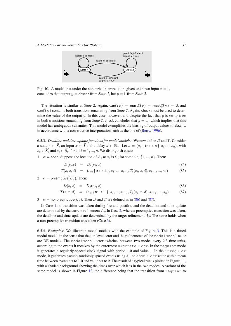
A Modular Formal Semantics for Ptolemy 37

Fig. 10. A model that under the non-strict interpretation, given unknown input x =⊥,concludes that output y = absent from State 1, but y =⊥ from State 2.

The situation is similar at State 2. Again, can(TP ) = must(TP ) = must(TN ) = ∅, andcan(TN ) contains both transitions emanating from State 2. Again, check must be used to deter-mine the value of the output y. In this case, however, and despite the fact that y is set to true

in both transitions emanating from State 2, check concludes that y = ⊥, which implies that thismodel has ambiguous semantics. This model exemplifies the biasing of output values to absent,in accordance with a constructive interpretation such as the one of (Berry, 1996).

6.5.3. Deadline and time-update functions for modal models: We now defineD and T . Considera state s ∈ S, an input x ∈ I and a delay d ∈ R+. Let s = (sc, {tr 7→ α}, s1, ..., sn), withsc ∈ Sc and si ∈ Si, for all i = 1, ..., n. We distinguish cases:

1 α = none. Suppose the location of Ac at sc is `i, for some i ∈ {1, ..., n}. Then:

D(s, x) = Di(si, x) (84)

T (s, x, d) = (sc, {tr 7→ ⊥}, s1, ..., si−1, Ti(si, x, d), si+1, ..., sn) (85)

2 α = preemptive(i, j). Then:

D(s, x) = Dj(sj , x) (86)

T (s, x, d) = (sc, {tr 7→ ⊥}, s1, ..., sj−1, Tj(sj , x, d), sj+1, ..., sn) (87)

3 α = nonpreemptive(i, j). Then D and T are defined as in (86) and (87).

In Case 1 no transition was taken during fire and postfire, and the deadline and time-updateare determined by the current refinement Ai. In Case 2, where a preemptive transition was taken,the deadline and time-update are determined by the target refinement Aj . The same holds whena non-preemptive transition was taken (Case 3).

6.5.4. Examples: We illustrate modal models with the example of Figure 3. This is a timedmodal model, in the sense that the top level actor and the refinements of the ModalModel actorare DE models. The ModalModel actor switches between two modes every 2.5 time units,according to the events it receives by the outermost DiscreteClock. In the regular modeit generates a regularly-spaced clock signal with period 1.0 and value 1. In the irregularmode, it generates pseudo-randomly spaced events using a PoissonClock actor with a meantime between events set to 1.0 and value set to 2. The result of a typical run is plotted in Figure 11,with a shaded background showing the times over which it is in the two modes. A variant of thesame model is shown in Figure 12, the difference being that the transition from regular to

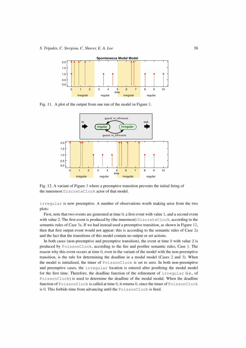
S. Tripakis, C. Stergiou, C. Shaver, E. A. Lee 38

irregular regularirregular regular

0.00.5

1.0

1.5

2.0

0 1 2 3 4 5 6 7 8 9 10

Spontaneous Modal Model

time

Fig. 11. A plot of the output from one run of the model in Figure 3.

irregular regularirregular regular

0.00.5

1.0

1.5

2.0

0 1 2 3 4 5 6 7 8 9 10

Spontaneous Modal Model

time

irregular regularirregular regular

0.00.5

1.0

1.5

2.0

0 1 2 3 4 5 6 7 8 9 10

Spontaneous Modal Model

time

Fig. 12. A variant of Figure 3 where a preemptive transition prevents the initial firing ofthe innermost DiscreteClock actor of that model.

irregular is now preemptive. A number of observations worth making arise from the twoplots:

First, note that two events are generated at time 0, a first event with value 1, and a second eventwith value 2. The first event is produced by (the innermost) DiscreteClock, according to thesemantic rules of Case 3a. If we had instead used a preemptive transition, as shown in Figure 12,then that first output event would not appear: this is according to the semantic rules of Case 2aand the fact that the transitions of this model contain no output or set actions.

In both cases (non-preemptive and preemptive transition), the event at time 0 with value 2 isproduced by PoissonClock, according to the fire and postfire semantic rules, Case 1. Thereason why this event occurs at time 0, even in the variant of the model with the non-preemptivetransition, is the rule for determining the deadline in a modal model (Cases 2 and 3). Whenthe model is initialized, the timer of PoissonClock is set to zero. In both non-preemptiveand preemptive cases, the irregular location is entered after postfiring the modal modelfor the first time. Therefore, the deadline function of the refinement of irregular (i.e., ofPoissonClock) is used to determine the deadline of the modal modal. When the deadlinefunction of PoissonClock is called at time 0, it returns 0, since the timer of PoissonClockis 0. This forbids time from advancing until the PoissonClock is fired.

A Modular Formal Semantics for Ptolemy 39

Another interesting observation concerns the output events with value 1 occurring at times 3.5,4.5, 8, and so on, in the plot of Figure 11. These events occur at times during which the model isat the regular mode. As explained above, the model begins in the regular mode but spendszero time there, since it immediately transitions to the irregularmode. In the non-preemptivecase, the DiscreteClock is postfired before entering irregular (Case 3d). Hence, thetimer of DiscreteClock has value 1 when irregular is entered. When regular is re-entered at time 2.5, this timer still has value 1, since it has not been updated in the meantime.It therefore expires one time unit later, i.e., at time 3.5, which explains the event at that time.Moreover, the timer is reset to 1 during postfire(). It expires again one time unit later, whichexplains the event at time 4.5. Finally, it is reset to 1 at time 4.5, suspended at time 5, andresumed at time 7.5, which explains the event at time 8.

Consider also the event with value 1 at time 2.5, in the plot of Figure 12. This event isgenerated when regular is re-entered at time 2.5. In the case of a preemptive transition,DiscreteClock has not been postfired at time 0, therefore, its timer has value 0 at time 2.5.This explains the event at that time.

7. Conclusions and Future Work

This paper proposes a formal semantics for the heterogeneous modeling environment Ptolemy.The semantics is modular in the sense that it unifies atomic and composite actors within a singleexecutable interface. Directors, which realize specific models of computation, are compositionoperators: they take as input a diagram of actors and return a new (composite) actor. Becausecomposite actors have the same interface as atomic actors, they can be seen as “black boxes”. Thisenables reasoning about a hierarchical model in a modular, actor-by-actor basis, thus minimizingthe complexity that arises from cross-cutting dependencies between levels of the hierarchy.

An implementation of our framework in the functional programming language Haskell is on-going. Prototype implementations of the SR, DE, CT and PN domains are currently available.Implementation of MM is under way. Our goal for the Haskell-based implementation is not tobe a replacement for the current Java implementation of Ptolemy (the primary reason being thebetter performance of the latter). Instead we intend to use it mainly as a tool for validating the se-mantics. This validation can be performed by comparing the results of the two implementationson different models. All the examples described in this paper, with the exception of the examplecontaining a modal model (Figure 3), have been modeled both in Ptolemy and in the Haskellimplementation, and give equivalent results, modulo minor numerical discrepancies.

Adding more models of computation to the collection presented in this paper is one of thedirections for future work. Another direction is to examine the properties of the directors ascomposition operators, for instance, properties related to associativity and commutativity. Wehope that this will lead to a better understanding of the properties of heterogeneous modelingin general. We also hope that this framework will serve as a starting point for a more in-depthdiscussion on how to unify different models of computation (for instance, which are the possibleactor interfaces and what are their relative merits?) as well as how to formally represent them(e.g., what would be the right language for writing directors?).

S. Tripakis, C. Stergiou, C. Shaver, E. A. Lee 40

References

Aiguier, M., Golden, B., and Krob, D. (2011). Complex Systems Modeling II: A minimalist and unifiedsemantics for heterogeneous integrated systems. Applied Mathematics and Computation. To appear.

Alur, R., Courcoubetis, C., Halbwachs, N., Henzinger, T. A., Ho, P.-H., Nicollin, X., Olivero, A., Sifakis,J., and Yovine, S. (1995). The algorithmic analysis of hybrid systems. Theor. Comput. Sci., 138:3–34.

Alur, R. and Dill, D. L. (1994). A theory of timed automata. Theoretical Computer Science, 126(2):183–235.

André, C. (1996). SyncCharts: A visual representation of reactive behaviors. Technical Report RR 95–52,rev. RR (96–56), I3S.

André, C. (2003). Semantics of S.S.M (Safe State Machine). Technical report, Esterel Technologies.Arbab, F. (2004). Reo: A channel-based coordination model for component composition. Mathematical

Structures in Computer Science, 14(3):329–366.Arnold, A. and Nivat, M. (1980). Metric interpretations of infinite trees and semantics of non deterministic

recursive programs. Fundamenta Informaticae, 11(2):181–205.Bae, K., Csaba Olveczky, P., Feng, T. H., Lee, E. A., and Tripakis, S. (Accepted for publication, Oct 2010).

Verifying Hierarchical Ptolemy II Discrete-Event Models using Real-Time Maude. Science of ComputerProgramming.

Baier, C. and Majster-Cederbaum, M. E. (1994). Denotational semantics in the CPO and metric approach.Theoretical Computer Science, 135(2):171–220.

Balarin, F., Hsieh, H., Lavagno, L., Passerone, C., Sangiovanni-Vincentelli, A. L., and Watanabe, Y. (2003).Metropolis: an integrated electronic system design environment. Computer, 36(4).

Basu, A., Bozga, M., and Sifakis, J. (2006). Modeling heterogeneous real-time components in BIP. InInternational Conference on Software Engineering and Formal Methods (SEFM), pages 3–12, Pune.

Beeck, M. v. d. (1994). A comparison of Statecharts variants. In Langmaack, H., de Roever, W. P., andVytopil, J., editors, 3rd Intl. Symp. Formal Techniques in Real-Time and Fault-Tolerant Systems, volume863 of LNCS, pages 128–148, Lübeck, Germany. Springer-Verlag.

Benveniste, A. and Berry, G. (1991). The synchronous approach to reactive and real-time systems. Pro-ceedings of the IEEE, 79(9):1270–1282.

Benveniste, A., Caspi, P., Edwards, S., Halbwachs, N., Le Guernic, P., and de Simone, R. (2003). Thesynchronous languages 12 years later. Proceedings of the IEEE, 91(1):64–83.

Benveniste, A., Caspi, P., Lublinerman, R., and Tripakis, S. (2009). Actors without directors: a Kahnianview of heterogeneous systems. In Hybrid Systems – Computation and Control (HSCC), volume LNCS.Springer.

Berry, G. (1996). The Constructive Semantics of Pure Esterel. Book Draft.Bliudze, S. and Krob, D. (2009). Modelling of complex systems: Systems as dataflow machines. Fundam.

Inf., 91:251–274.Bliudze, S. and Sifakis, J. (2008a). The algebra of connectors - structuring interaction in bip. IEEE Trans.

Computers, 57(10):1315–1330.Bliudze, S. and Sifakis, J. (2008b). A notion of glue expressiveness for component-based systems. In van

Breugel, F. and Chechik, M., editors, CONCUR 2008, volume 5201 of LNCS, pages 508–522. Springer.Boulanger, F., Hardebolle, C., Jacquet, C., and Marcadet, D. (2011). Semantic Adaptation for Models of

Computation. In Proceedings of ACSD 2011 (Application of Concurrency to System Design), pages153–162. IEEE Computer Society.

Bozga, M., Sfyrla, V., and Sifakis, J. (2009). Modeling synchronous systems in BIP. In Chakraborty, S.and Halbwachs, N., editors, EMSOFT, pages 77–86. ACM.

Broy, M. and Stolen, K. (2001). Specification and Development of Interactive Systems, volume 62 ofMonographs in Computer Science. Springer.

A Modular Formal Semantics for Ptolemy 41

Bruneton, E., Coupaye, T., Leclercq, M., Quéma, V., and Stefani, J.-B. (2006). The FRACTAL componentmodel and its support in Java. Softw. Pract. Exper., 36:1257–1284.

Buck, J. T. (1993). Scheduling Dynamic Dataflow Graphs with Bounded Memory Using the Token FlowModel. Ph.d. thesis, University of California, Berkeley.

Buck, J. T., Ha, S., Lee, E. A., and Messerschmitt, D. G. (1994). Ptolemy: A framework for simulating andprototyping heterogeneous systems. Int. Journal of Computer Simulation, special issue on “SimulationSoftware Development”, 4:155–182.

Burch, J. R., Passerone, R., and Sangiovanni-Vincentelli, A. L. (2001). Overcoming heterophobia: Model-ing concurrency in heterogeneous systems. In International Conference on Application of Concurrencyto System Design, page 13.

Cataldo, A., Lee, E., Liu, X., Matsikoudis, E., and Zheng, H. (2006). A constructive fixed-point theoremand the feedback semantics of timed systems. In Proceedings of the 8th International Workshop onDiscrete-Event Systems (WODES’06).

Damm, W., Josko, B., Hungar, H., and Pnueli, A. (1998). A Compositional Real-time Semantics of STATE-MATE Designs. In Compositionality: The Significant Difference, volume 1536 of LNCS, pages 186–238.Springer.

Davey, B. A. and Priestley, H. A. (2002). Introduction to Lattices and Order. Cambridge University Press,2nd edition.

Denckla, B. and Mosterman, P. (2008). Stream- and state-based semantics of hierarchy in block diagrams.In 17th IFAC World Congress, pages 7955–7960.

Dijkstra, E. W. (1976). A Discipline of Programming. Prentice Hall.Dill, D. L. (1988). Trace theory for automatic hierarchical verification of speed-independent circuits. Ph.d.,

Carnegie-Mellon University.Edwards, S. A. and Lee, E. A. (2003). The semantics and execution of a synchronous block-diagram

language. Science of Computer Programming, 48(1).Eker, J., Janneck, J. W., Lee, E. A., Liu, J., Liu, X., Ludvig, J., Neuendorffer, S., Sachs, S., and Xiong, Y.

(2003). Taming heterogeneity—the Ptolemy approach. Proceedings of the IEEE, 91(2):127–144.Eshuis, R. (2009). Reconciling statechart semantics. Sci. Comput. Program., 74(3):65–99.Feredj, M., Boulanger, F., and Mbobi, A. M. (2009). A model of domain-polymorph component for hetero-

geneous system design. The Journal of Systems and Software, 82:112–120.Floyd, R. W. (1967). Assigning meaning to programs. In Proc. of Symposium on Applied Mathematics,

volume 19, pages 19–32. A.M.S.Geilen, M. and Basten, T. (2003). Requirements on the execution of Kahn process networks. In European

Symposium on Programming Languages and Systems, LNCS, pages 319–334. Springer.Geilen, M. and Basten, T. (2004). Reactive process networks. In 4th ACM international conference on

Embedded Software, EMSOFT ’04, pages 137–146. ACM.Goderis, A., Brooks, C., Altintas, I., Lee, E. A., and Goble, C. (2009). Heterogeneous composition of

models of computation. Future Generation Computer Systems, 25(5):552 – 560.Goessler, G. and Sangiovanni-Vincentelli, A. (2002). Compositional modeling in Metropolis. In Second

International Workshop on Embedded Software (EMSOFT), Grenoble, France. Springer-Verlag.Graf, S., Ober, I., and Ober, I. (2006). A real-time profile for UML. Soft. Tools Tech. Transfer, 8(2):113–127.Gurevich, Y. (1993). Evolving algebras: An attempt to discover semantics. In Rozenberg, G. and Salomaa,

A., editors, Current Trends in Theoretical Computer Science, pages 266–292. World Scientific.Halbwachs, N., Caspi, P., Raymond, P., and Pilaud, D. (1991). The synchronous data flow programming

language LUSTRE. Proceedings of the IEEE, 79(9):1305–1319.Hamon, G. (2005). A denotational semantics for stateflow. In EMSOFT ’05: Proceedings of the 5th ACM

international conference on Embedded software, pages 164–172, New York, NY, USA. ACM.

S. Tripakis, C. Stergiou, C. Shaver, E. A. Lee 42

Hamon, G. and Rushby, J. (2004). An operational semantics for Stateflow. In Fundamental Approaches toSoftware Engineering (FASE), volume 2984 of LNCS, pages 229–243, Barcelona, Spain. Springer.

Hardebolle, C., Boulanger, F., Marcadet, D., and Vidal-Naquet, G. (2007). A generic execution frame-work for models of computation. In Proceedings of the Fourth International Workshop on Model-BasedMethodologies for Pervasive and Embedded Software, MOMPES ’07, pages 45–54, Washington, DC,USA. IEEE Computer Society.

Harel, D. (1987). Statecharts: A visual formalism for complex systems. Science of Computer Programming,8:231–274.

Herrera, F. and Villar, E. (2006). A framework for embedded system specification under different modelsof computation in SystemC. In Design Automation Conference (DAC), San Francisco. ACM.

Jantsch, A. (2003). Modeling Embedded Systems and SoCs - Concurrency and Time in Models of Compu-tation. Morgan Kaufmann.

Kahn, G. (1974). The semantics of a simple language for parallel programming. In Proc. of the IFIPCongress 74. North-Holland Publishing Co.

Karsai, G. (1995). A configurable visual programming environment: A tool for domain-specific program-ming. IEEE Computer, pages 36–44.

Kohavi, Z. (1978). Switching and finite automata theory. McGraw-Hill.Ledeczi, A., Bakay, A., Maroti, M., Volgyesi, P., Nordstrom, G., Sprinkle, J., and Karsai, G. (2001). Com-

posing domain-specific design environments. IEEE Computer, pages 44–51.Lee, E. A. (1999). Modeling concurrent real-time processes using discrete events. Annals of Software

Engineering, 7:25–45.Lee, E. A. (2009). Finite State Machines and Modal Models in Ptolemy II. Technical Report UCB/EECS-

2009-151, EECS Department, University of California, Berkeley.Lee, E. A. (2010). Disciplined heterogeneous modeling. In D.C. Petriu, N. Rouquette, O. H., editor,

Proceedings of the ACM/IEEE 13th International Conference on Model Driven Engineering, Languages,and Systems (MODELS), pages 273–287. IEEE.

Lee, E. A. and Matsikoudis, E. (2009). The semantics of dataflow with firing. In Huet, G., Plotkin, G.,Lévy, J.-J., and Bertot, Y., editors, From Semantics to Computer Science: Essays in memory of GillesKahn. Cambridge University Press.

Lee, E. A. and Messerschmitt, D. G. (1987). Synchronous data flow. Proceedings of the IEEE, 75(9):1235–1245.

Lee, E. A. and Parks, T. M. (1995). Dataflow process networks. Proceedings of the IEEE, 83(5):773–801.Lee, E. A. and Sangiovanni-Vincentelli, A. (1998). A framework for comparing models of computation.

IEEE Transactions on Computer-Aided Design of Circuits and Systems, 17(12):1217–1229.Lee, E. A. and Tripakis, S. (2010). Modal Models in Ptolemy. In EOOLT 2010 – 3rd International Workshop

on Equation-Based Object-Oriented Modeling Languages and Tools. Linköping University ElectronicPress.

Lee, E. A. and Zheng, H. (2005). Operational semantics of hybrid systems. In Morari, M. and Thiele,L., editors, Hybrid Systems: Computation and Control (HSCC), volume LNCS 3414, pages pp. 25–53,Zurich, Switzerland. Springer-Verlag.

Lee, E. A. and Zheng, H. (2007). Leveraging synchronous language principles for heterogeneous modelingand design of embedded systems. In EMSOFT, Salzburg, Austria. ACM.

Liu, J. and Lee, E. A. (2003). On the causality of mixed-signal and hybrid models. In 6th InternationalWorkshop on Hybrid Systems: Computation and Control (HSCC ’03), Prague, Czech Republic.

Liu, X. and Lee, E. A. (2008). CPO semantics of timed interactive actor networks. Theoretical ComputerScience, 409(1):110–125.

Liu, X., Matsikoudis, E., and Lee, E. A. (2006). Modeling timed concurrent systems. In CONCUR 2006 -Concurrency Theory, volume LNCS 4137, Bonn, Germany. Springer.

A Modular Formal Semantics for Ptolemy 43

Lublinerman, R., Szegedy, C., and Tripakis, S. (2009). Modular Code Generation from Synchronous BlockDiagrams – Modularity vs. Code Size. In 36th ACM SIGPLAN-SIGACT Symposium on Principles ofProgramming Languages (POPL’09), pages 78–89. ACM.

Malik, S. (1994). Analysis of cyclic combinational circuits. IEEE Trans. Computer-Aided Design,13(7):950–956.

Manna, Z. and Pnueli, A. (1992). Verifying hybrid systems. Hybrid Systems, pages 4–35.Maraninchi, F. and Bhouhadiba, T. (2007). 42: Programmable models of computation for a component-

based approach to heterogeneous embedded systems. In 6th ACM International Conference on Genera-tive Programming and Component Engineering (GPCE), pages 1–3, Salzburg, Austria.

Maraninchi, F. and Rémond, Y. (2003). Mode-automata: a new domain-specific construct for the develop-ment of safe critical systems. Sci. Comput. Program., 46:219–254.

Meyer, B. (1992). Applying "design by contract". Computer, 25(10):40–51.Nordstrom, G., Sztipanovits, J., Karsai, G., and Ledeczi, A. (1999). Metamodeling - rapid design and

evolution of domain-specific modeling environments. In Proc. of Conf. on Engineering of ComputerBased Systems (ECBS), pages 68–74, Nashville, Tennessee.

Patel, H. D. and Shukla, S. K. (2004). SystemC Kernel Extensions for Heterogeneous System Modelling.Kluwer.

Reed, G. M. and Roscoe, A. W. (1988). Metric spaces as models for real-time concurrency. In 3rd Workshopon Mathematical Foundations of Programming Language Semantics, pages 331–343, London, UK.

Sander, I. and Jantsch, A. (2004). System modeling and transformational design refinement in ForSyDe.IEEE Transactions on Computer-Aided Design of Circuits and Systems, 23(1):17–32.

Scaife, N., Sofronis, C., Caspi, P., Tripakis, S., and Maraninchi, F. (2004). Defining and Translating a“Safe” Subset of Simulink/Stateflow into Lustre. In Proceedings of the 4th ACM Intl. Conf. on EmbeddedSoftware (EMSOFT’04), pages 259–268. ACM.

Shiple, T., Berry, G., and Touati, H. (1996). Constructive analysis of cyclic circuits. In European Designand Test Conference (EDTC’96). IEEE Computer Society.

Sifakis, J. (1977). Use of petri nets for performance evaluation. In Measuring, modelling and evaluatingcomputer systems, pages 75–93. North-Holland.

Simon, G., Kovácsházy, T., and Péceli, G. (2000). Transient management in reconfigurable systems. InIWSAS’ 2000: Proc. 1st Intl. Workshop on Self-Adaptive Software, pages 90–98, Secaucus, NJ, USA.Springer.

Sztipanovits, J., Wilkes, D., Karsai, G., Biegl, C., and Lynd, L. (1993). The multigraph and structuraladaptivity. IEEE Trans. Signal Proc., pages 2695–2716.

Tripakis, S., Bui, D., Geilen, M., Rodiers, B., and Lee, E. A. (Accepted for publication, Dec 2010). Com-positionality in Synchronous Data Flow: Modular Code Generation from Hierarchical SDF Graphs.ACM Transactions on Embedded Computing Systems (TECS). Preprint available as a technical re-port from http://www.eecs.berkeley.edu/Pubs/TechRpts/2009/EECS-2009-143.

html.Yates, R. K. (1993). Networks of real-time processes. In Best, E., editor, Proc. of the 4th Int. Conf. on

Concurrency Theory (CONCUR), volume LNCS 715. Springer-Verlag.Zhu, Y., Westbrook, E., Inoue, J., Chapoutot, A., Salama, C., Peralta, M., Martin, T., Taha, W., O’Malley, M.,

Cartwright, R., Ames, A., and Bhattacharya, R. (2010). Mathematical equations as executable models ofmechanical systems. In Proceedings of the 1st ACM/IEEE International Conference on Cyber-PhysicalSystems, ICCPS ’10, pages 1–11. ACM.