A Molecular Modeling Approach to Predicting Thermo-Mechanical

Properties of Thermosetting Polymers

Natalia Shenogina, Wright State University Mesfin Tsige, University of Akron

Soumya Patnaik, AFRL Sharmila Mukhopadhyay, Wright State University

June 5, 2012

Thermoset Polymers

Applications – Aerospace composites

– Other structural materials

– Adhesives

– Encapsulation and boards for electronics

Properties that enable these applications – Dimensional stability

– Thermal stability

– Mechanical Strength

– Chemical resistance

– Electrical Properties

Polymer

Unique Opportunities/Challenges Variability in Structures and Properties

• All polymers are prone to structural variations and

thermosets have additional variable introduced by curing step.

• However, these are important materials, having annual market demand well over $15B worldwide.

• Thousands of variations that have been empirically tailored for specific needs.

Computational Models can make tailoring easier and more

economical by systematically predicting composition-structure-property relationships.

Predictive Models for Macromolecules

Models operate at different levels of detail: – Length scales

– Time Scales

– Degrees of freedom

– Etc….

Practical considerations: – Number of constraints

– Number of unknowns

– Realistic Conditions

– Computational time

Ref: Florian Muller-Plathe , SOFT MATERIALS, Vol. 1, pp. 1–31, 2003

Scales in Modeling

• Finite-element methods (FEM) are widely used to study large-scale events in polymers.

– Often limited by lack of the realistic parameters for inputs to constitutive relations.

– These parameters can be difficult to obtain from experiments.

• Molecular Dynamics (MD) simulations can provide detailed microscopic information.

• Can provide parameters for larger systems (finite element analysis or coarse-grained models)

• The coarse-grained simulations in turn can be used as a guidance for the all atom (AA) simulations

MD simulations of Thermosetting Polymers (TSP)

• Several reported MD simulations have demonstrated that it can be successfully used as a tool in predicting material properties of TSP.

• Various approaches of simulating bond formation and cross-linking have been developed to bring models closer to experimental conditions.

• Some Issues remain: – Many obtained structures have low degree of curing – Some have high internal stresses and distortions – Number of atoms that can be included have been small, typically

less than 15K atoms These issues often lead to predicted properties that are far from those of

real systems

Objectives of this study

• Construct more realistic models

• Achieve high degree of cure, closer to engineering materials.

• Calculate some of the important material properties, and compare with experimental trends:

– Density

– Glass transition temperature

– Coefficient of thermal expansion

– Elastic constants

• Investigate influence of simulation size, extent of curing, and length of epoxy strands on these quantities.

Long-term Goals

• Use of atomistic MD predicted parameters to incorporate into larger scale models (coarse-grained etc.)

• Provide parameters for constitutive relations in Finite Element Methods

• Allow prediction of the strength and toughness as a function of experimental parameters such as: monomer chemistry, cross-link density and temperature

Simulation Predictions (Tsige et al)

Tensile tests on similar chemistry (Mukhopadhyay et al)

In future, better

correlations between these

Polymer System Investigated Epoxy-amine cured system: reactants

• Epoxy resin: DGEBA (diglycidyl ether of bisphenol A) – Functionality: 2

• Aromatic amine

hardener: DETDA (diethylene toluene diamine) – Functionality: 4

Epoxy-amine cured system: amorphous cell

Stochiometric ratio of epoxy resin and hardener (32/16 molecules) in a box

resin hardener atoms

32 16 ~2000

64 32 ~4000

96 48 ~6000

128 64 ~8000

256 128 ~15000

432 216 ~23000

512 256 ~35000

General Approach Used

• All simulations performed using Materials Studio package from Accelrys.

• Generate epoxy-amine systems cured to a given extent of reaction

• Study volume-temperature behavior:

– Density, Glass transition temperature, Coefficients of thermal expansion

• Estimate elastic properties:

– Young’s, Shear and Bulk Modulus, Poisson’s ratio

Details at: Shenogina, N.; Tsige, M.; Patnaik, S.; Mukhopadhyay, S. , “Molecular Modeling Approach to Prediction of Thermo-Mechanical Behavior of Thermoset Polymer Networks”, Macromolecules, accepted for publication, 2012

Building of Thermosets

• Generate many topologically independent structures

• Extract energetic and structural information at each cross-linking cycle on-the fly.

• Maximum bond stretching energy considered as a good measure of distortion.

• Models that show dramatic increase of maximum bond stretching energy at high extent of reaction are rejected (signifies artificially high stresses )

0.0 0.2 0.4 0.6 0.8-20

0

20

40

60

80

100

120

140

160

180

Ma

xim

um

bo

nd

en

erg

y,

kc

al/

mo

l

Extent of reaction 0.0 0.2 0.4 0.6 0.8 1.00.4

0.6

0.8

1.0

1.2

1.4

1.6

Ma

xim

um

bo

nd

en

erg

y,

kc

al/

mo

l

Extent of reaction

rejected accepted

I. Thermal Property Calculations

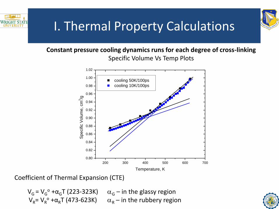
VG = VGo +αGT (223-323K)

VR= VRo +αRT (473-623K)

Coefficient of Thermal Expansion (CTE)

aG – in the glassy region aR – in the rubbery region

200 300 400 500 600 700

0.80

0.82

0.84

0.86

0.88

0.90

0.92

0.94

0.96

0.98

1.00

1.02

Sp

ecific

Vo

lum

e, cm

3/g

Temperature, K

cooling 50K/100ps

cooling 10K/100ps

Constant pressure cooling dynamics runs for each degree of cross-linking Specific Volume Vs Temp Plots

Analysis of the V vs. T plots (100% curing)

Experimental values: Density: 1.16 g/cm3 (Ratna et al, J. Mater. Sci. 38, 147-154 (2003)) Tg: 443 K (Jansen et al, Polymer, 40, 5601-5607 (1999)) 457 K (Ratna et al, Poly. Int. 52, 1403-1407 (2003)) 441 K (Shen et al, Macromol. Mat. Eng. 291 (2006) 476 K (Liu et al, Polymer, 47, 2091-2098 (2006)) aG: 24*10-5/K (Liu et al, Polymer, 47, 2091-2098 (2006))

structure Dens.(298K) g/cm3

Dens.(480K) g/cm3

Tg,K αG 1/K *10-5

αR 1/K *10-5

1 1.138 1.089 363 17.0 27.4

2 1.122 1.092 562 21.4 34.2

3 1.137 1.107 471 12.9 52.5

4 1.142 1.107 462 14.2 49.2

5 1.160 1.097 370 14.2 40.6

average 1.140 1.098 446 15.9 40.8

Coefficient of Thermal Expansion (CTE) as a function of degree of cross-link

•CTE decreases with increasing degree of curing •Size effect is detected, larger structures show clearly linear trend

T=480K

T=298K

50 60 70 80 90 10010

20

30

40

50

60

70

Vo

lum

etr

ic c

oe

ff.o

f th

erm

.exp

an

sio

n*1

0-5, 1

/K

Extent of reaction,%

2000 atoms

4000 atoms

6000 atoms

8000 atoms

15000 atoms

23000 atoms

34000 atoms

Exp. value

CTE for different chain lengths of epoxy

•The dependence of CTE on degree of curing decreases with chain length

T=480K

T=298K

50 60 70 80 90 100

20

30

40

50

60

70

Vo

lum

etr

ic c

oe

ff.o

f th

erm

.exp

an

sio

n*1

0-5,1

/K

Extent of reaction,%

1 monomer

2 monomers

4 monomers

Variation of Tg with degree of curing

Tg increases with degree of curing, within range of experimental values

50 60 70 80 90 100380

400

420

440

460

480

Gla

ss tra

nsitio

n te

mp

era

ture

, K

Extent of reaction,%

2000 atoms

4000 atoms

6000 atoms

8000 atoms

15000 atoms

23000 atoms

34000 atoms

Exp. values

Density variation with degree of curing

•Density increases with degree of curing •This effect is more pronounced at higher temperature

T=298K

T=480K

50 60 70 80 90 100

1.02

1.04

1.06

1.08

1.10

1.12

1.14

1.16

1.18

1.20

De

nsity, g

/cm

3

Extent of reaction,%

2000 atoms

4000 atoms

6000 atoms

8000 atoms

15000 atoms

23000 atoms

34000 atoms

Exp. value

Role of chain length of the epoxy strands on density

•Density increases with chain length

T=298K

T=480K

50 60 70 80 90 100

1.02

1.04

1.06

1.08

1.10

1.12

1.14

1.16

1.18

1.20

De

nsity,g

/cm

3

Extent of reaction,%

1 monomer

2 monomers

4 monomers

Mechanical Properties

• Any small (e.g. nanometer scale) volume element of an amorphous

material can be characterized by unique distribution of matter.

• Individual elements viewed as regions.

• A large number of such elements averaged using Voigt-Reuss and Hill-Walpole approaches.

• Finally, assuming isotropic symmetry, Lame elastic constants obtained from stress and compliance tensors. Leads to coomonly measured coefficents: – Young’s modulus

– Shear Modulus

– Bulk Modulus

– Poisson’s ratio

Mechanical Properties

Static Approach

• Static approach (Theodoru and Suter, 1986): – Neglect entropic contributions to elastic response – Take into account potential energy contribution – Small deformations and low temperatures

• Three tensile and three shear deformations of magnitude ±0.001 are applied to the system

• Energy minimization of the structures

• The obtained stress tensor is then used to estimate stiffness coefficients of the material

• Elastic constants are calculated: Young’s, bulk, shear moduli, Poisson’s ratio

Young’s modulus vs. degree of curing Static Approach

Experimental value is 2.71GPa, lower than simulations [Qi et al, Compos. Struct. 75, 514-519 (2006)]: tensile test at room temperature

T=298K

T=480K

50 60 70 80 90 100

3

4

5

6

7

8

9

10

Yo

un

g's

mo

du

lus, G

Pa

Extent of reaction,%

6000 atoms

8000 atoms

15000 atoms

23000 atoms

35000 atoms

Young’s modulus vs. degree of curing for different chain lengths (static Approach)

•The rate of increase depends on chain length

50 60 70 80 90 1004

5

6

7

8

9

Yo

un

g's

mo

du

lus,G

Pa

Extent of reaction,%

1 monomer

2 monomers

4 monomers

T=298K

T=480K

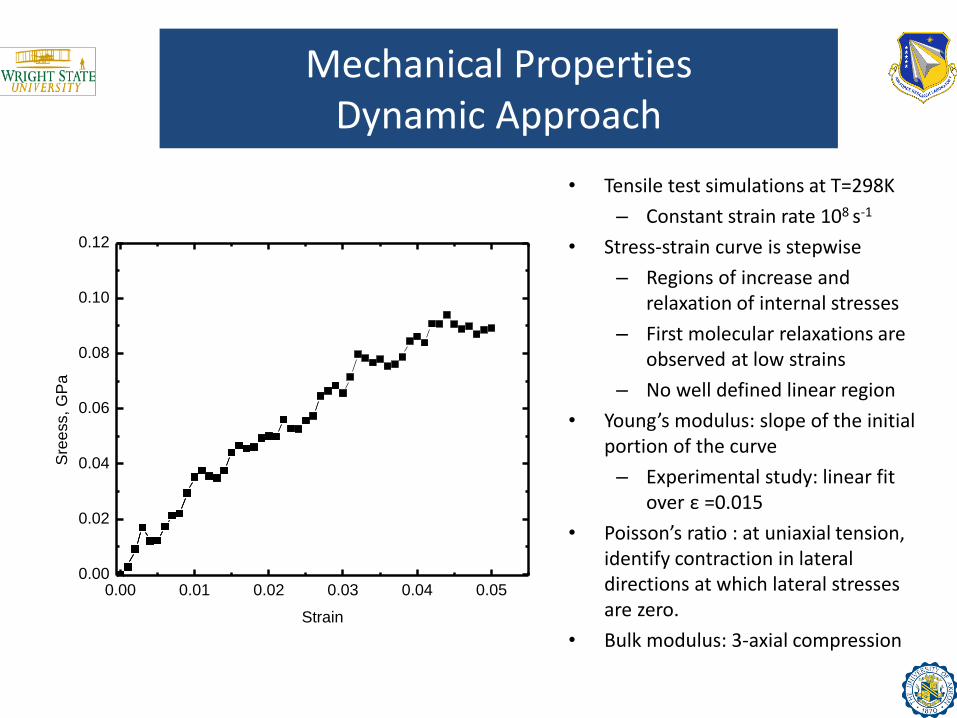
Mechanical Properties Dynamic Approach

• Tensile test simulations at T=298K

– Constant strain rate 108 s-1

• Stress-strain curve is stepwise

– Regions of increase and relaxation of internal stresses

– First molecular relaxations are observed at low strains

– No well defined linear region

• Young’s modulus: slope of the initial portion of the curve

– Experimental study: linear fit over ε =0.015

• Poisson’s ratio : at uniaxial tension, identify contraction in lateral directions at which lateral stresses are zero.

• Bulk modulus: 3-axial compression

0.00 0.01 0.02 0.03 0.04 0.050.00

0.02

0.04

0.06

0.08

0.10

0.12

Sre

ess, G

Pa

Strain

Poisson’s ratio vs. degree of curing Dynamic vs. Static Approach

T=480K, dynamic

T=298K, dynamic

T=298K, static

T=480K, static

Exp. value

Poisson’s ratio predictions significantly approved by dynamic approach

50 60 70 80 90 100

0.28

0.30

0.32

0.34

0.36

0.38

0.40

0.42

0.44

0.46

0.48

Po

isso

n's

Ra

tio

Degree of Curing, %

Young’s modulus vs. degree of curing. Dynamic vs. Static Approach

T=298K, static

T=480K, static

T=298K, dynamic

T=480K, dynamic

Exp. value

•Dynamic effects seem to provide much more realistic predictions. •This is despite large strain rates and small sizes, inherent to MD

50 60 70 80 90 100

0

1

2

3

4

5

6

7

8

You

ng

's M

od

ulu

s, G

Pa

Degree of Curing, %

Bulk modulus vs. degree of curing Dynamic vs. Static Approach (compression)

T=298K, static

T=480K, static

T=298K, dynamic

T=480K, dynamic

50 60 70 80 90 100

1

2

3

4

5

6

7

Bu

lk M

od

ulu

s, G

Pa

Degree of Curing, %

Shear modulus vs. degree of curing Dynamic vs. Static Approach

T=298K, static

T=480K, static

T=298K, dynamic

T=480K, dynamic

50 60 70 80 90 100

0

1

2

3

4

5

She

ar

Mo

du

lus, G

Pa

Degree of Curing, %

Summary

Stress free thermo-set models up to 35000 atoms were generated with high degree of cure containing

Densities, CTE and Tg were found in good agreement with

experimental data Effects of system size and chain length investigated

Mechanical Deformation has been simulated using both static and dynamic approaches and their results compared. Significant improvements are seen by treating this as a dynamic event

Publications and Presentations to date

Papers:

• Shenogina, N.; Tsige, M.; Patnaik, S.; Mukhopadhyay, S.M, “Molecular Modeling Approach to Prediction of Thermo-Mechanical Behavior of Thermoset Polymer Networks”, Macromolecules, 2012.

• N. B. Shenogina, M. Tsige, S. M. Mukhopadhyay, S. S. Patnaik, “Molecular modeling of thermosetting polymers: effects of degree of curing and chin length on thermo-mechanical properties” , Proceedings of 18th International Conference on Composite Materials, August, 2011.

• Shenogina, N.; Tsige, M.; Patnaik, S.; Mukhopadhyay, S.M .“Molecular Modeling to Predict Elastic Properties of Highly Cross-linked Polymer Networks Using Dynamic Deformation Approach”, to be submitted to Macromolecules.

Book Chapter:

• S. S. Patnaik and M. Tsige, “Modeling and Simulation of Nanoscale Materials” Chapter 6 in Nanoscale Multifunctional Materials, Science and Applications, Edited by S. M. Mukhopadhyay, Wiley, 2012.

Conferences:

• N.Shenogina, M.Tsige, S.Patnaik, S.M. Mukhopadhyay “Molecular Dynamics Simulations of Mechanical Behavior of Thermosetting Polymers” Dayton-Cincinnati Aerospace Sciences Symposium, March , 2011

• N.Shenogina, M.Tsige, S.M. Mukhopadhyay, S.Patnaik “A Molecular Modeling Approach to Predicting Thermo-Mechanical Properties of Thermosetting Polymers”, US National Congress on Computational Mechanics-11, July, 2011

• N.Shenogina, M.Tsige, S.M.Mukhopadhyay, S.Patnaik “Molecular Modeling Simulations of Highly Cross-linked Polymer Networks: Prediction of Thermal and Mechanical Properties”, American Physical Society March Meeting, March, 2012

• M. Tsige, N.Shenogina, S.Patnaik, S.M. Mukhopadhyay , “Molecular Modeling Simulations of Highly Cross-linked Polymer Networks”, Invited Presentation, 10th International Symposium of Polymer Physics, May 2012, Chengdou, China.

Acknowledgements

• Financial support from AFOSR

Program Manager: Dr. Joycelyn Harrison

• Valuable discussions with Dr. Charles Lee

• Computer Time: DoD Supercomputing Resource Center High Performance Computing.

Thank you!

Mechanical Properties Simulation Basic Theory

• The isothermal elastic constants are defined as the elements of the 4th rank tensor of the second derivatives of the Helmholtz energy per unit volume, equivalent to the first derivative of the stress with respect to strain, i.e.

• For small deformations stress and strain are related by

• where C denote the stiffness coefficients, and S the compliance coefficients of the material

Mechanical Properties Basic Theory (cont’d)

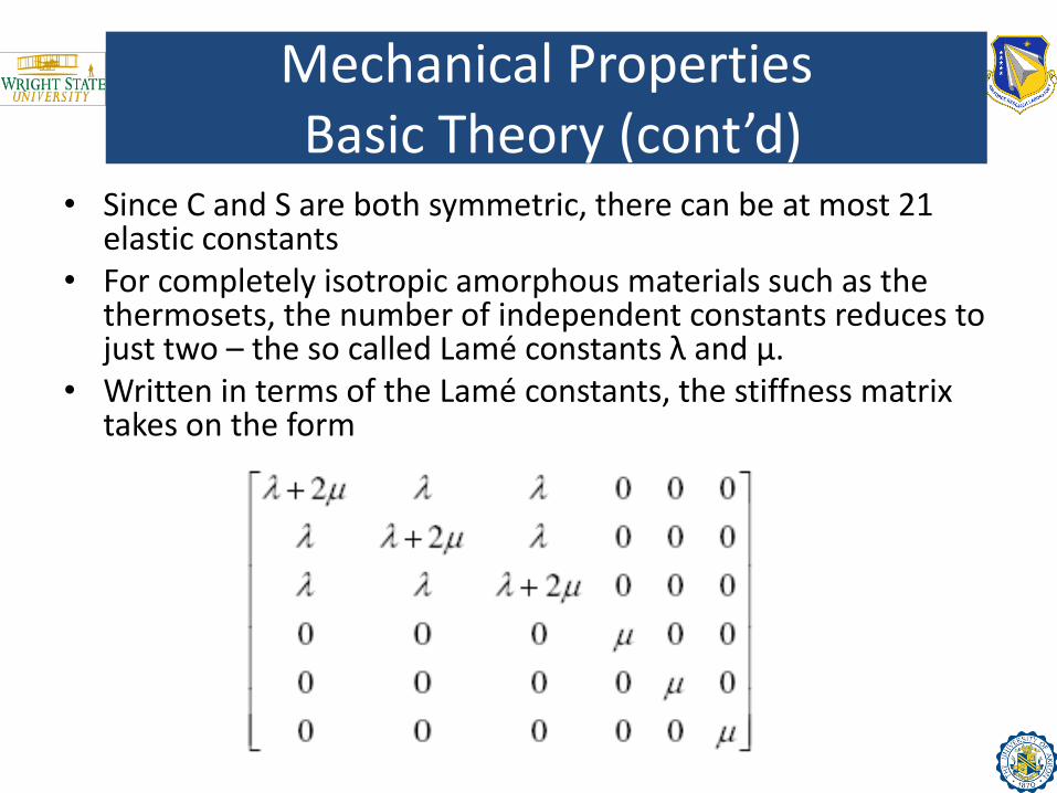
• Since C and S are both symmetric, there can be at most 21 elastic constants

• For completely isotropic amorphous materials such as the thermosets, the number of independent constants reduces to just two – the so called Lamé constants λ and μ.

• Written in terms of the Lamé constants, the stiffness matrix takes on the form

Mechanical PropertiesTheory (cont’d)

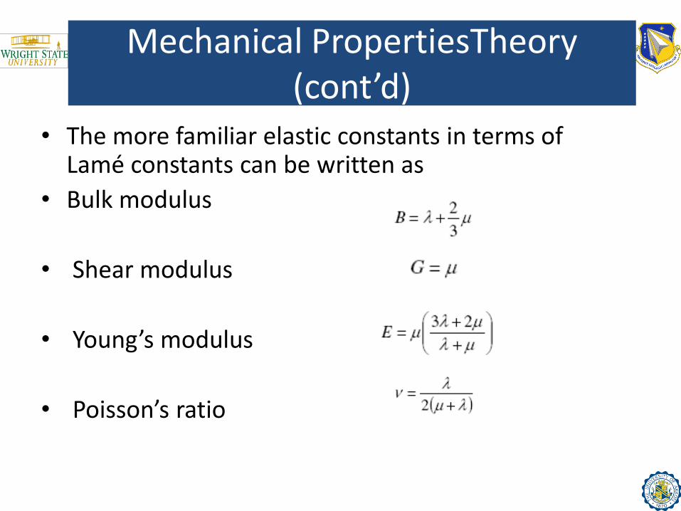
• The more familiar elastic constants in terms of Lamé constants can be written as

• Bulk modulus

• Shear modulus

• Young’s modulus

• Poisson’s ratio

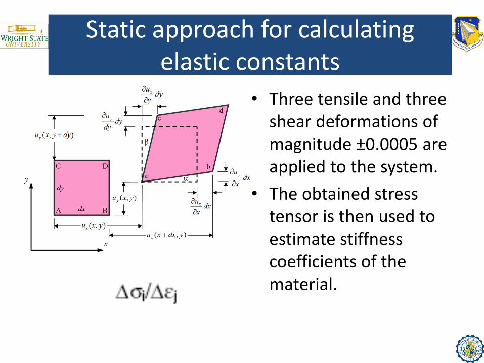
Static approach for calculating elastic constants

• Three tensile and three shear deformations of magnitude ±0.0005 are applied to the system.

• The obtained stress tensor is then used to estimate stiffness coefficients of the material.

Mechanical Properties Theory – Bounds Calculation

• Any small (e.g. nanometer scale) volume element of an amorphous material can be characterized by unique distribution of matter within it.

• Individual elements can be viewed as regions of a nanoscopically heterogeneous composite material.

• Distribution of the material properties in the macroscopic sample.

• Upper and lower bounds of the elastic constants of such material can be estimated by considering averages of the individual stiffness and compliance matrices of the elements. Thus we obtain the so-called Voigt and Reuss bounds

Mechanical Properties Theory – Bounds Calculation(cont’d)

• For typical simulated systems, the difference between Voigt and Reuss bounds can be 10-20% of the mean.

• To calculate mechanical properties of the thermosets with similar characteristics (e.g. hardeners or extents of reaction) we need improved (narrower) bounds estimates.

• Hill and Walpole approach can be used to obtain the improved bounds of the elastic constants

Mechanical Properties Theory – Hill-Walpole Bounds Calculation

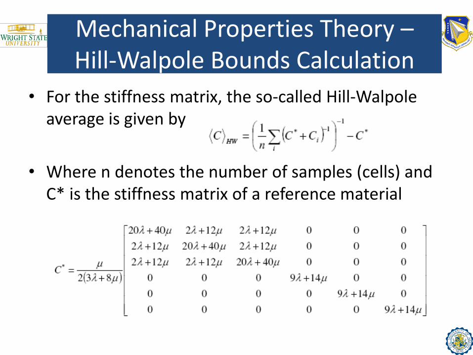
• For the stiffness matrix, the so-called Hill-Walpole average is given by

• Where n denotes the number of samples (cells) and C* is the stiffness matrix of a reference material

Mechanical Properties Theory – Hill-Walpole Bounds Calculation(cont’d)

• Two moduli, say B and G, are calculated for the stiffness matrix obtained for each model

• The extremes of these values over the full set of models are then used to define four comparison matrices by combining (Bmax,Gmax), (Bmin,Gmin), (Bmax,Gmin), (Bmin,Gmax)

• The 4 comparison matrices are used to generate 4 Hill-Walpole averages <C>HW and the associated sets of moduli {B, G, E, ν}

• Extreme values of the 4 sets of moduli are taken to define the Hill-Walpole bounds