Auton RobotDOI 10.1007/s10514-012-9294-z

A momentum-based balance controller for humanoid robotson non-level and non-stationary ground

Sung-Hee Lee · Ambarish Goswami

Received: 14 October 2011 / Accepted: 10 April 2012© Springer Science+Business Media, LLC 2012

Abstract Recent research suggests the importance of con-trolling rotational dynamics of a humanoid robot in bal-ance maintenance and gait. In this paper, we present a novelbalance strategy that controls both linear and angular mo-mentum of the robot. The controller’s objective is definedin terms of the desired momenta, allowing intuitive controlof the balancing behavior of the robot. By directly deter-mining the ground reaction force (GRF) and the center ofpressure (CoP) at each support foot to realize the desiredmomenta, this strategy can deal with non-level and non-stationary grounds, as well as different frictional propertiesat each foot-ground contact. When the robot cannot realizethe desired values of linear and angular momenta simultane-ously, the controller attributes higher priority to linear mo-mentum at the cost of compromising angular momentum.This creates a large rotation of the upper body, reminiscentof the balancing behavior of humans. We develop a com-putationally efficient method to optimize GRFs and CoPs atindividual foot by sequentially solving two small-scale con-strained linear least-squares problems. The balance strategyis demonstrated on a simulated humanoid robot under ex-periments such as recovery from unknown external pushesand balancing on non-level and moving supports.

Electronic supplementary material The online version of this article(doi:10.1007/s10514-012-9294-z) contains supplementary material,which is available to authorized users.

S.-H. LeeSchool of Information and Communications, Gwangju Institute ofScience and Technology, Gwangju, South Koreae-mail: shl@gist.ac.kr

A. Goswami (�)Honda Research Institute, Mountain View, CA, USAe-mail: agoswami@honda-ri.com

Keywords Humanoid robot balance · Linear and angularmomentum · Non-level ground · Momentum control ·Centroidal momentum matrix

1 Introduction

Even after several decades of research balance maintenancehas remained one of the most important issues of humanoidrobots. Although the basic dynamics of balance are currentlyunderstood, robust and general controllers that can deal withdiscrete and non-level foot support as well as large, unex-pected and unknown external disturbances such as movingsupport, slip and trip have not yet emerged. Especially, incomparison with the elegance and versatility of human bal-ance, present-day robots appear quite deficient. In order forhumanoid robots to coexist with humans in the real world,more advanced balance controllers that can deal with a broadrange of environment conditions and external perturbationsneed to be developed.

Until recently, most balance control techniques have at-tempted to maintain balance by controlling only the linearmotion of a robot. For example, Kagami et al. (2000) andKudoh et al. (2002) proposed methods to change the inputjoint angle trajectories to modify the position of the Centerof Pressure (CoP), a point within the robot’s support areathrough which the resultant Ground Reaction Force (GRF)acts. When the CoP, computed from the input joint motion,leaves the support base, indicating a possible toppling of afoot, the motion is modified to bring the CoP back inside thesupport base while the robot still follows the desired linearmotion of the Center of Mass (CoM). The rotational mo-tion of the robot remains more or less ignored in these ap-proaches.

Auton Robot

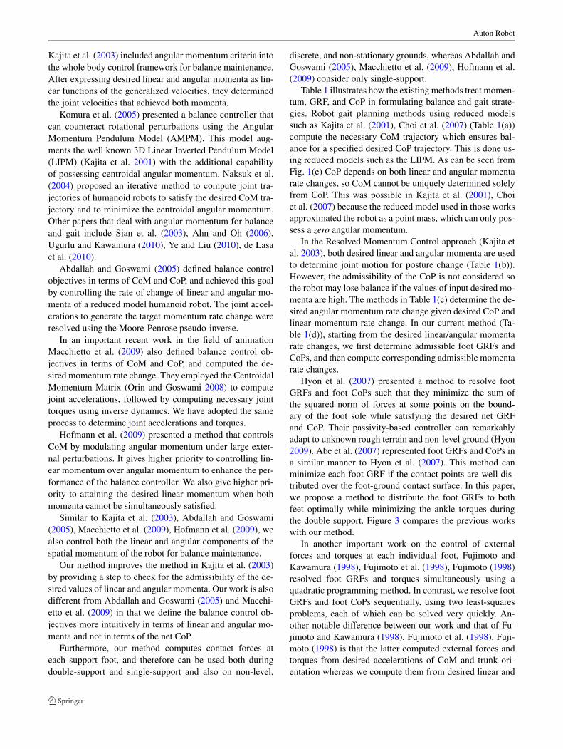
Fig. 1 The external forces and torques in (a) are solely responsiblefor the centroidal momentum rate change in (b). (c): Linear momen-tum rate change l has a one-to-one correspondence with the GRF f .(d): The centroidal angular momentum rate change k is determined byboth f and CoP location p. (e): Conversely, p is determined by both l

and k

However, rotational dynamics of a robot plays a signifi-cant role in balance (Komura et al. 2005). Experiments onhuman balance control also show that humans tightly reg-ulate angular momentum during gait (Popovic et al. 2004),which suggests the strong possibility that angular momen-tum may be important in humanoid movements.

In fact, both angular and linear momenta must be regu-lated to completely control the CoP. The fundamental quan-tities and the relations between them are schematically de-picted in Fig. 1 and described subsequently.

Figure 1(a) shows all the external forces that act on afreely standing humanoid: the GRF f , the Ground ReactionMoment τn normal to the ground, and the weight mg of therobot, where m is the total robot mass and g is the acceler-ation due to gravity. According to D’Alembert’s principle,the sums of external moments and external forces, respec-tively, are equivalent to the rates of change of angular andlinear momenta, respectively, of the robot. The mathemati-cal expressions for these relationships are given by (1) and(2). Figure 1(b) depicts the robot’s rate of change of angu-lar momentum about the CoM, k, and linear momentum, l,respectively.

k = (p − rG) × f + τn (1)

l = mg + f (2)

In the above equations, rG is the CoM location and p isthe CoP location. Together k and l is a 6 × 1 vector calledthe spatial centroidal momentum h = [kT lT ]T , which wasstudied in Orin and Goswami (2008). In this paper, we willcall it spatial momentum, or simply the momentum of therobot. The aggregate momentum of a humanoid robot maybe obtained by summing up all of the angular and linear mo-menta contributed by the individual link segments. The cen-troidal momentum is this aggregate momentum of the robot

projected to a reference point instantaneously located at itsCoM. Note that the spatial centroidal momentunm is com-puted with respect to a frame which is aligned to the worldframe and located at the overall CoM of the robot. Also theframe is instantaneously frozen with respect to the worldframe.

Indeed, as noted in Macchietto et al. (2009), the (spa-tial) momentum rate change has a one-to-one relationshipwith the GRF and CoP. From (2) and as shown in Fig. 1(c),l is completely determined by f and vice versa. Further-more, from (1) and Fig. 1(d), a complete description of k

needs both f and p. Conversely, p depends on both k andl, which is shown in Fig. 1(e).1 This last sentence impliesthat a complete control of p is impossible without control-ling both momenta.

Based on this fundamental relation researchers have de-veloped balance maintenance methods that controls boththe linear and angular components of the spatial momen-tum (Kajita et al. 2003; Abdallah and Goswami 2005;Macchietto et al. 2009). We will call balance controllers ofthis approach momentum-based balance controllers.

Some momentum-based balance control approaches de-fine the desired rotational behavior of the controller in termsof the CoP (Abdallah and Goswami 2005; Macchietto etal. 2009) while others use angular momentum (Kajita et al.2003). Although the GRF-CoP combination has a one-to-one relationship with momentum rate changes, their signifi-cance regarding balance are very different, and is worth dis-cussing. Whereas the former characterize the magnitude, di-rection and point of application of the external forces, thelatter describes the resulting motion of a robot. The unilat-eral nature of robot-ground contact and friction limits im-pose important direct constraints on the range of GRF andCoP. These influence the achievable range of momentumrate change, but only indirectly. On the other hand, it is morenatural to describe the aggregate motion of a robot in termsof momentum.

In this paper we present a new momentum-based balancecontroller that uses both the momentum and the GRF-CoPfor their respectively appropriate purposes: We use momen-tum to define control objectives as well as to compute jointmotions while GRF and CoP are used as constraints.

In this method, we first specify the desired momentumrate change for balance (Sect. 3.2). However, the desiredmomentum rate change may not always be physically real-izable due to several constraints on the foot-ground contact.

1The normal torque τn also affects k in the transverse plane. Actu-ally f , p, and τn together constitute the 6 variables that correspond tothe 6 variables of the spatial momentum. Usually τn is omitted in thediscussion for simplicity because its magnitude is small.

Auton Robot

Fig. 2 Overview of Momentum-Based Balance Controller. θu

d is thedesired joint accelerations for the upper body. T d,i and vd,i are thedesired configuration and spatial velocity of each foot (i = r, l). Sub-scripts d and a imply “desired” and “admissible,” respectively

First, the CoP cannot be outside the robot’s support base.2

Second, the GRF must be unilateral in nature, and can neverattract the robot towards the ground. Third, the GRF mustsatisfy the friction limit of the foot-ground surface, so as notto cause slip.

Therefore, in the next step we determine the admissiblevalues of GRF and CoP that will create the desired momen-tum rate change as close as possible while being physicallyrealizable. Specifically, in order to make the controller ro-bustly applicable to non-level and non-stationary ground,we directly determine admissible foot GRFs and foot CoPs,without using more conventional net GRF and net CoP ofthe robot. Assuming planar contact between the ground andeach foot, the foot GRF is the ground reaction force actingon an individual foot and foot CoP is the location where itsline of action intersects the foot support plane. Using thevalues of admissible foot GRF and foot CoP we recalculatemomentum rate changes – these are the admissible momen-tum rate changes (Sect. 3.4).

In the subsequent step we resolve the joint accelerationsgiven the admissible momentum rate change, desired jointaccelerations for the upper body, and desired motion of thefeet. Finally we compute necessary joint torques to createthe joint accelerations and the admissible external forces us-ing inverse dynamics (Sect. 3.5). Figure 2 shows the blockdiagram for the controller.

During double support, the computation of foot GRFsand foot CoPs from the desired momentum rate change isan under-determined problem. This allows us to pursue anadditional optimality criterion in the solution. In this paper,we minimize the ankle torques while generating the desiredmomentum rate change. Minimizing ankle torque is impor-tant because typically the ankle torque is more constrainedthan others in that it should not cause foot tipping.

Specifically, we show that computing optimal foot GRFsand foot CoPs that minimizes ankle torques can be achieved

2During single support, the support base is identical to the foot contactarea, whereas during double support on level ground, the support baseis equivalent to the convex hull of the support areas of the two feet.

by solving two simple constrained linear least-squares prob-lems. Our simulation experiments show that this new opti-mization method is significantly faster than the conventionalquadratic programming approach to solve the same problem.

The main unique contributions of this paper can be listedas follows:

1. Our momentum-based control framework determines thedesired momenta but before attempting to reach them, itfirst checks to make sure that the momenta targets arephysically attainable by computing their admissible val-ues.

2. The optimal foot GRFs and foot CoPs are computedquickly by solving two small-scale linear least-squaresproblems.

3. The framework is sufficiently general to support amomentum-based stepping algorithm, as reported re-cently (Yun and Goswami 2011).

We will present a number of simulation experiments in-cluding pushing the single or double-supported robot in var-ious directions, and maintaining balance when two feet areon separate moving supports with different inclinations andvelocities.

The remainder of this paper is organized as follows. Afterdiscussing related work in Sect. 2, we detail the momentum-based balance control framework in Sect. 3. Section 4 re-ports the simulation experiments. Section 5 provides the dis-cussion and the future work.

2 Related work

Starting from the early work of Vukobratovic and Juricic(1969), researchers have developed numerous techniquesfor biped balance control using various approaches. Amongthese are joint control strategies using ankle or hip (Sanoand Furusho 1990; Stephens 2007), whole body control ap-proaches (Kagami et al. 2000; Sugihara et al. 2002; Kajitaet al. 2003; Choi et al. 2007; Park et al. 2005; Stephensand Atkeson 2010), methods that find optimal control poli-cies (Zhou and Meng 2003; Muico et al. 2009), and reflexcontrollers (Huang and Nakamura 2005). In this section wefocus on the research relevant to momentum-based balancecontrol.

The importance of angular momentum in humanoidwalking was reported by Sano and Furusho as early as1990 (Sano and Furusho 1990). However, it was muchlater before its importance for balance maintenance ofhuman and humanoid robots started to be seriously ex-plored (Kajita et al. 2003; Goswami and Kallem 2004;Popovic et al. 2004). Sano and Furusho (1990), and Mi-tobe et al. (2004) showed that it is possible to generate thedesired angular momentum by controlling the ankle torque.

Auton Robot

Kajita et al. (2003) included angular momentum criteria intothe whole body control framework for balance maintenance.After expressing desired linear and angular momenta as lin-ear functions of the generalized velocities, they determinedthe joint velocities that achieved both momenta.

Komura et al. (2005) presented a balance controller thatcan counteract rotational perturbations using the AngularMomentum Pendulum Model (AMPM). This model aug-ments the well known 3D Linear Inverted Pendulum Model(LIPM) (Kajita et al. 2001) with the additional capabilityof possessing centroidal angular momentum. Naksuk et al.(2004) proposed an iterative method to compute joint tra-jectories of humanoid robots to satisfy the desired CoM tra-jectory and to minimize the centroidal angular momentum.Other papers that deal with angular momentum for balanceand gait include Sian et al. (2003), Ahn and Oh (2006),Ugurlu and Kawamura (2010), Ye and Liu (2010), de Lasaet al. (2010).

Abdallah and Goswami (2005) defined balance controlobjectives in terms of CoM and CoP, and achieved this goalby controlling the rate of change of linear and angular mo-menta of a reduced model humanoid robot. The joint accel-erations to generate the target momentum rate change wereresolved using the Moore-Penrose pseudo-inverse.

In an important recent work in the field of animationMacchietto et al. (2009) also defined balance control ob-jectives in terms of CoM and CoP, and computed the de-sired momentum rate change. They employed the CentroidalMomentum Matrix (Orin and Goswami 2008) to computejoint accelerations, followed by computing necessary jointtorques using inverse dynamics. We have adopted the sameprocess to determine joint accelerations and torques.

Hofmann et al. (2009) presented a method that controlsCoM by modulating angular momentum under large exter-nal perturbations. It gives higher priority to controlling lin-ear momentum over angular momentum to enhance the per-formance of the balance controller. We also give higher pri-ority to attaining the desired linear momentum when bothmomenta cannot be simultaneously satisfied.

Similar to Kajita et al. (2003), Abdallah and Goswami(2005), Macchietto et al. (2009), Hofmann et al. (2009), wealso control both the linear and angular components of thespatial momentum of the robot for balance maintenance.

Our method improves the method in Kajita et al. (2003)by providing a step to check for the admissibility of the de-sired values of linear and angular momenta. Our work is alsodifferent from Abdallah and Goswami (2005) and Macchi-etto et al. (2009) in that we define the balance control ob-jectives more intuitively in terms of linear and angular mo-menta and not in terms of the net CoP.

Furthermore, our method computes contact forces ateach support foot, and therefore can be used both duringdouble-support and single-support and also on non-level,

discrete, and non-stationary grounds, whereas Abdallah andGoswami (2005), Macchietto et al. (2009), Hofmann et al.(2009) consider only single-support.

Table 1 illustrates how the existing methods treat momen-tum, GRF, and CoP in formulating balance and gait strate-gies. Robot gait planning methods using reduced modelssuch as Kajita et al. (2001), Choi et al. (2007) (Table 1(a))compute the necessary CoM trajectory which ensures bal-ance for a specified desired CoP trajectory. This is done us-ing reduced models such as the LIPM. As can be seen fromFig. 1(e) CoP depends on both linear and angular momentarate changes, so CoM cannot be uniquely determined solelyfrom CoP. This was possible in Kajita et al. (2001), Choiet al. (2007) because the reduced model used in those worksapproximated the robot as a point mass, which can only pos-sess a zero angular momentum.

In the Resolved Momentum Control approach (Kajita etal. 2003), both desired linear and angular momenta are usedto determine joint motion for posture change (Table 1(b)).However, the admissibility of the CoP is not considered sothe robot may lose balance if the values of input desired mo-menta are high. The methods in Table 1(c) determine the de-sired angular momentum rate change given desired CoP andlinear momentum rate change. In our current method (Ta-ble 1(d)), starting from the desired linear/angular momentarate changes, we first determine admissible foot GRFs andCoPs, and then compute corresponding admissible momentarate changes.

Hyon et al. (2007) presented a method to resolve footGRFs and foot CoPs such that they minimize the sum ofthe squared norm of forces at some points on the bound-ary of the foot sole while satisfying the desired net GRFand CoP. Their passivity-based controller can remarkablyadapt to unknown rough terrain and non-level ground (Hyon2009). Abe et al. (2007) represented foot GRFs and CoPs ina similar manner to Hyon et al. (2007). This method canminimize each foot GRF if the contact points are well dis-tributed over the foot-ground contact surface. In this paper,we propose a method to distribute the foot GRFs to bothfeet optimally while minimizing the ankle torques duringthe double support. Figure 3 compares the previous workswith our method.

In another important work on the control of externalforces and torques at each individual foot, Fujimoto andKawamura (1998), Fujimoto et al. (1998), Fujimoto (1998)resolved foot GRFs and torques simultaneously using aquadratic programming method. In contrast, we resolve footGRFs and foot CoPs sequentially, using two least-squaresproblems, each of which can be solved very quickly. An-other notable difference between our work and that of Fu-jimoto and Kawamura (1998), Fujimoto et al. (1998), Fuji-moto (1998) is that the latter computed external forces andtorques from desired accelerations of CoM and trunk ori-entation whereas we compute them from desired linear and

Auton Robot

Table 1 The diagrams show how each method on balance control orgait pattern generation treats momenta (k, l), GRF (f ), and CoP (p).A pair of solid lines determines the target value together. The dottedline shows the determination process of linear motion and force. The

subscript “d” indicates a desired input to the controller and superscript“∗” indicates that the quantity is used to determine control output suchas joint torques

(a) Kajita et al. (2001), Choi etal. (2007)

(b) Kajita et al. (2003) (c) Abdallah and Goswami(2005), Macchietto et al. (2009)

(d) Lee and Goswami (2010), thispaper

Fig. 3 Comparison of the optimal foot GRFs given the same net GRF(f ) and CoP (p) between Hyon et al. (2007), Abe et al. (2007) and ourmethod. The figure shows the robot feet and the shanks in the coronalplane. The ankle joints are not precisely located at the center of thefeet due to the mechanical design considerations. The eccentricity isdenoted by d . (a): The method presented in Hyon et al. (2007), Abe etal. (2007): Minimizing the sum of squared norms of the contact forcesat sample points (marked with circles on the foot bottoms) results inhaving the foot GRFs at the center of the foot bottoms and inducesankle torques. (b): Our method: Minimizing both (1) the difference ofthe magnitudes of foot GRFs and (2) the ankle torques results in zeroankle torques in the case shown above

angular momenta rate changes. The advantage of computingdesired trunk orientation from external forces and torques isthat it can be done more intuitively than computing desiredangular momentum, the latter having no direct visible refer-ence. On the other hand, our approach is based on Newton’slaw, i.e., momentum rate change is completely determinedby the external forces and torques. In contrast, the angularacceleration of the trunk cannot be completely determinedfrom the external forces and torques unless the accelera-tions of other joints are also specified. If these joint acceler-ations are not incorporated in the force/torque computation,the computed values would be valid only for motions withnegligible joint accelerations.

Sentis et al. (2010) developed a method to precisely con-trol contact CoPs in a more general setting of multicontactinteraction between a humanoid robot and the environmentusing a virtual-linkage model. Park et al. (2007) showed thatmany balancing problems can be framed as the second-ordercone programming problem.

Unlike the above-mentioned approaches which involvedistributing the net GRF and net CoP to the supporting feet,

Sugihara and Nakamura (2003), Sugihara (2003) take a dif-ferent approach that computes the desired acceleration ofCoM from the desired foot GRFs and foot CoPs, and thenresolves the joint motion to realize the desired accelerationof CoM.

This method has the merit of offering an easy manipula-tion of contact state between individual foot and the groundbut, as mentioned in Sugihara and Nakamura (2003), Sugi-hara (2003) by the authors themselves, is not guaranteed torealize the desired foot CoP and GRF during double support.

3 Momentum-based balance control framework

This is the main section of the paper which provides step-by-step details of how the joint torques for the controller aredetermined.

3.1 Control framework

We will represent the configuration of a humanoid robotas Q = (T 0, θ) ∈ SE(3) × R

n, where T 0 = (R0,p0) ∈SO(3) × R

3 denotes the base frame (trunk) configuration,θ ∈ R

n is the vector of joint angles, and n is the total num-ber of joint DoFs. The subscripts 0 and s denote the baseframe and joints, respectively, with s implying “shape” as-sociated with the joint angles in geometric dynamics (Blochet al. 1996). The total DoFs of the robot is thus 6 + n, be-cause the floating base has 6 DoFs. The generalized velocitycan be written as q = (v0, θ) ∈ R

6+n where v0 = (ω0,υ0)

is the spatial velocity of the trunk with respect to the bodyframe and expressed as: 3

[ω0]× = RT0 R0 (3)

υ0 = RT0 p0 (4)

3q is a slight abuse of notation because we do not define nor use avector q . However, since se(3), the Lie algebra of SE(3), is isomorphicto R

6, we will use a single vector form of q ∈ R6+n for convenience.

[ω0]× represents a skew-symmetric matrix of a vector ω0.

Auton Robot

Then, assuming stationary ground, the constraint equationsdue to ground contacts and the joint space equations of mo-tion of the robot are as follows:

0 = J (Q)q (5)

τ = H (Q)q + C(Q, q)q + τ g(Q) − J T f c (6)

where τ ∈ R6+n denotes the generalized forces, H is the

joint space inertia matrix, Cq includes Coriolis and cen-trifugal terms and τ g is the gravity torque. f c is a vectorrepresenting external “constraint” forces from the ground,determined by foot GRFs and CoPs, and the Jacobian J ∈R

c×(6+n) transforms f c to the generalized forces. The num-ber of constraint equations c depends on the nature of con-straint at the foot-ground contact. For example, when boththe linear and angular motion of the support foot are con-strained due to foot-ground contact, c = 6 for single supportand c = 12 for double support. In this case, J q denotes thelinear and angular velocities of the support foot given q , and0 in (5) denotes zero velocity of the support foot.

Since the robot base is free floating, the first six elementsof τ are zero, i.e., τT = [0T τT

s ]. Hence, we can divide (6)into two parts, one corresponding to the base, denoted by thesubscript 0, and the other, subscripted with s, for the joints.Then (5) and (6) are rewritten as follows:

0 = J q + J q (7)

0 = H 0q + C0q + τ g,0 − J T0 f c (8)

τ s = H s q + Cs q + τg,s − J Ts f c (9)

where (7) is the time derivative of (5).Due to the high DoFs of humanoid robots, balance con-

trollers usually solve an optimization problem. However, thecomputational cost of the optimization increases rapidly asthe dimension of the search space increases. Even the sim-plest optimization problem such as the least-squares prob-lem has order O(n3) time complexity. Therefore, aimingfor computational efficiency, we have adopted a sequentialapproach; we divide the balance control problem into threesmaller sub-problems, which can be solved serially. The bal-ance controller determines the control input τ s through thefollowing steps:

– Step 1: foot GRFs and foot CoPs (hence f c) are com-puted from the desired momentum rate change.

– Step 2: joint accelerations q are determined such that theysatisfy both (7) and (8). Actually, as will be explained inSect. 3.5, instead of directly using (8), we use the cen-troidal momentum equation (32), which is a slight varia-tion of (8). In general, if the total number of robot DoFsis greater than or equal to c + 6, a solution to q exists.

– Step 3: the required joint torques τ s satisfying (9) arecomputed from f c and q using an inverse dynamics al-gorithm.

Note that, by computing f c and q first, we can useefficient linear-time algorithms for inverse dynamics inStep 3, without having to compute the joint space equa-tions of motion (6) which have a quadratic time complex-ity.

3.2 Desired momentum for balance control

The overall behavior of the robot against external perturba-tions is determined by the desired momentum rate change.We employ the following feedback control policy:

kd = Γ 11(kd − k) (10)

ld/m = Γ 21(rG,d − rG) + Γ 22(rG,d − rG) (11)

where kd and ld are the independently specified desiredrates of change of centroidal angular and linear momenta.In other words kd and ld are not time derivatives of kd andld . Additionally, rG,d is the desired CoM position. Γ ij rep-resents 3×3 diagonal matrix of feedback gain parameters.Note that unlike the linear position feedback term in (11),we do not have an angular position feedback in (10). Thisis because a physically meaningful angular “position” can-not be defined corresponding to angular momentum (Wieber2005). For postural balance maintenance experiments we setkd and rG,d to zero and rG,d to be above the mid-point ofthe geometric centers of the two feet. For other cases, thesevalues may be determined from the desired motion.

It is to be noted that, despite the various studies onangular momentum in humanoid motions (Komura et al.2005; Popovic et al. 2004; Sano and Furusho 1990; Ka-jita et al. 2003; Mitobe et al. 2004; Naksuk et al. 2004;Goswami and Kallem 2004; Abdallah and Goswami 2005;Ahn and Oh 2006; Macchietto et al. 2009; Hofmann etal. 2009; Ugurlu and Kawamura 2010; Ye and Liu 2010;de Lasa et al. 2010), the issue of how to set the desired angu-lar momentum for more complex motions such as locomo-tion has not been fully explored, and remains an importantfuture work.

3.3 Prioritization between linear and angular momenta

Given the desired momentum rate change, we determine ad-missible foot GRF and foot CoP such that the resulting mo-mentum rate change is as close as possible to the desiredvalue. If the desired GRF and CoP computed from kd and ldviolate physical constraints (e.g., GRF being outside frictioncone, normal component of GRF being negative, or CoP be-ing outside support base), it is not possible to generate thosekd and ld . In this case we must strike a compromise and de-cide which quantity out of kd and ld is more important topreserve.

Auton Robot

Fig. 4 When the desired GRF, f d and the desired CoP, pd computedfrom the desired momentum rate change are not simultaneously ad-missible, as indicated by pd being outside the support base, momentaobjectives need to be compromised for control law formulation. Twoextreme cases are illustrated. Left: linear momentum is respected whileangular momentum is compromised. Right: angular momentum is re-spected while linear momentum is compromised

Figure 4 illustrates one case where the desired CoP,pd , computed from the desired momentum rate change isoutside the support base, indicating that it is not admissi-ble. Two different solutions are possible. The first solution,shown in Fig. 4, left, is to translate the CoP to the closestpoint of the support base while keeping the magnitude andline of action of the desired GRF f d unchanged. In this casethe desired linear momentum is attained but the desired an-gular momentum is compromised. The behavior emergingfrom this choice is characterized by a trunk rotation. Thisstrategy can be observed in the human when the trunk yieldsin the direction of the push to maintain balance. Alterna-tively, in addition to translating the CoP to the support base,as before, we can rotate the direction of the GRF, as shownin Fig. 4, right. In this case the desired angular momentumis attained while the desired linear momentum is compro-mised. With this strategy the robot must move linearly alongthe direction of the applied force due to the residual linearmomentum, making it necessary to step forward to preventfalling.

In this paper, we give higher priority to preserving lin-ear momentum over angular momentum because it in-creases the capability of postural balance without involv-ing a stepping. Ideally, a smart controller should be ableto choose optimal strategies depending on the environ-ment conditions and the status of the robot. The approachesthat give higher priority to linear momentum and sacri-fice angular momentum can also be found in the litera-ture (Hofmann et al. 2009; Stephens and Atkeson 2010)and in our recent work on stepping (Yun and Goswami2011).

3.4 Admissible foot GRF, foot CoP, and momentum ratechange

Given the desired momentum rate change, we determine ad-missible foot GRF and CoP such that the resulting momen-tum rate change is as close as possible to the desired value.Admissible momentum rate change is determined by the ad-missible foot GRF and foot CoP.

3.4.1 Single support case

Dealing with single support case is straightforward becausethe foot GRF and CoP are uniquely determined from thedesired momentum rate change, from (1) and (2):

f d = ld − mg (12)

pd,X = rG,X − 1

ld,Y − mg(fd,X rG,Y − kd,Z) (13)

pd,Z = rG,Z − 1

ld,Y − mg(fd,Z rG,Y + kd,X) (14)

where the Y -axis is parallel to the direction of gravity vector,i.e., g = (0, g,0).

If f d and pd computed above are valid, then we directlyuse these values. Otherwise, as mentioned previously, wegive higher priority to linear momentum. If f d is outside thefriction cone, we project it onto the friction cone to preventfoot slipping.

3.4.2 Double support case

Determining foot GRFs and foot CoPs for double support ismore involved. Let us first rewrite (1) and (2) for the dou-ble support case. Following Sano and Furusho (1990), wewill express the GRF at each foot in terms of the forcesand torques applied to the corresponding ankle (Fig. 5). Thebenefit of this representation is that we can explicitly expressthe torques applied to the ankles.

k = kf + kτ (15)

kf = (rr − rG) × f r + (r l − rG) × f l (16)

kτ = τ r + τ l (17)

l = mg + f r + f l (18)

In (15), we have divided k into two parts, kf , due to the an-kle force, and kτ , due to ankle torque. This division enablesus to take ankle torques into account in determining footGRFs. f r and f l are the GRFs at the right and left foot, re-spectively, and rr , r l are the positions of the body frames ofthe foot, located at the respective ankle joints.

Auton Robot

Fig. 5 By expressing GRF applied to each foot with respect to thelocal frame of the foot located at the ankle, we can factor out the mo-ments τ r , τ l applied to the ankle by the foot GRFs f r and f l . rr andr l are the positions of the ankles

Fig. 6 We represent the foot/ground interaction forces on the right footusing foot CoP, whose location with respect to the right foot frame {R}is denoted by dr = (dr,X,dr,Y ,−h), ground reaction moment normalto the ground τn,r = (0,0, τn,r ), and the GRF f r . f r is representedusing four basis vectors βrj (j = 1 . . .4) that approximate the frictioncone of the ground, i.e., f r = ∑

j βrj ρrj , where ρrj (≥ 0) is the mag-nitude in the direction of βrj . Therefore, the ground pressure is definedby 7 parameters, (ρr1, . . . , ρr4, dr,X, dr,Y , τn,r ). This representation iscompact, having only one more parameter than the minimum (3 forforce and 3 for torque), and constraint can be expressed in a very sim-ple form for a rectangular convex hull of the foot sole, i.e., ρj ≥ 0,dj ≤ dj ≤ dj , and |τn| < μτ fr,N where fr,N is the normal component

of f r , i.e., the Z-coordinate of RTr f r with Rr being the orientation of

the right foot. μτ is a friction coefficient for torque and h is the heightof foot frame from the foot sole. Note that dr and τn,r are expressedwith respect to the body frame {R} while rr , pr , f r , and βrj are withrespect to the world frame

The ankle torques τ i , (i = r, l) are expressed in terms offoot GRF and foot CoP as follows (Fig. 6):

τ i = (Rid i ) × f i + Riτn,i , (19)

where Ri is the orientation of the foot, d i is the foot CoPin body frame, and τn,i = (0,0, τn,i) is the normal torque inbody frame.

Given k and l, solving for foot GRFs and foot CoPs is anunderdetermined problem, which lets us prescribe additionaloptimality criteria to find a solution. If we incorporate min-imal ankle torques into the optimality condition, we could

express the objective function as follows:

wl

∥∥ld − l(f r ,f l )

∥∥2 + wk

∥∥kd − k(f r ,f l ,τ r ,τ l )

∥∥2

+ wf

(‖f r‖2 + ‖f l‖2) + wτ

(‖τ r‖2 + ‖τ l‖2)

s.t. f i and τ i are admissible (20)

where the first two terms aim to achieve the desired momen-tum rate change, the third term regularizes foot GRFs, andthe last term tries to minimize ankle torques. w’s are weight-ing factors among the different objectives.

Equation (20) represents a nonlinear and non-quadraticoptimization problem and it especially contains nonlinearcross product terms (see (19)); this makes it difficult to usein a real-time controller. One solution is to convert thisgeneral nonlinear optimization problem to easier ones thatcan be solved using least-squares or quadratic programmingmethods. This can be achieved by expressing the foot GRFand foot CoP using the forces at certain specific locations onthe boundary of the foot soles (Pollard and Reitsma 2001;Hyon et al. 2007). However, this approach increases the di-mension of the search space significantly. For example, Pol-lard and Reitsma (2001) used 16 variables to model the GRFand CoP of one foot, which is 10 more than the dimensionof the unknowns.

We develop a different approach. Instead of increasingthe search space to make the optimization problem eas-ier, we approximate (20) with two constrained least-squaresproblems, one for determining the foot GRFs, and the otherfor determining the foot CoPs. This way the number of vari-ables is kept small. Additionally, we attempt to minimizethe ankle torques. Minimizing ankle torques is meaningfulbecause large ankle torques can cause foot slipping.

Our approach can be intuitively understood as follows. Inorder to minimize the ankle torques (kτ → 0), the foot GRFsf r and f l should create kf as close to the desired angularmomentum rate change (kf → kd ) as possible while satisfy-ing ld . If kf = kd , the ankle torques can vanish. If kf �= kd ,we compute the ankle torques that are necessary to gener-ate the residual angular momentum rate change, kd − kf .In other words, by reducing burdens on the ankle torques tocreate kd , our approach can be understood as solving (20)for the case in which minimizing ankle torques has higherpriority than regularizing foot GRFs.

Determination of foot GRFs In order to compute the footGRFs, f r and f l , we solve the optimization problem below:

min∥∥ld − l(f r ,f l)

∥∥2 + wk

∥∥kd − kf (f r ,f l )

∥∥2

+ εf

(‖f r‖2 + ‖f l‖2), (21)

where wk and εf (wk εf > 0) are weighting factors forangular momentum and the regularization of foot GRFs, re-

Auton Robot

spectively. Note that, if kd = kf , the ankle torques τ i be-come zero. Each foot GRF is modeled using four basis vec-tors βij and their magnitudes ρij that approximate the fric-tion cone (an inverted pyramid in Fig. 6) on the ground

f i =4∑

j=1

β ij ρij := β iρi , (22)

where βi = [β i1 · · ·βi4].Note that rr and r l are determined by the configuration

of the robot; they are constants when solving this problem.Therefore kf becomes a linear equation of ρi when we sub-stitute (22) into (16). Rearranging into a matrix equation, wecan turn the optimization problem (21) into a linear least-squares problem with non-negativity constraints where theonly unknowns are the ρi :

min ‖Φρ − ξ‖2 s.t. ρi ≥ 0, (23)

where4

Φ =⎡

⎣βr β l

wf δr wf δl

εf 1

⎤

⎦ ∈ R(3+3+8)×(4+4) (24)

ξ =⎡

⎣ld − mg

wf kd

0

⎤

⎦ ∈ R(3+3+8)

ρ = [ρT

r ρTl

]T ∈ R8 (25)

δi = [r i − rG]×β i (26)

Determination of foot CoPs In general, the desired angu-lar momentum rate change cannot be fully generated only byf r and f l , so the residual, kτ,d = kd − kf , should be gen-erated by the ankle torques. To this end, we determine thelocation of each foot CoP such that they create kτ,d whileminimizing each ankle torque. It is to be noted that, afterhaving determined f i , (19) can be written as a linear func-tion of d i and τn,i :

τ i = −[f i]×Rid i + Riτn,i , (27)

so that we can express the optimization problem as a least-squares problem with upper and lower bounds:

min ‖Ψ η − κ‖2 s.t. η ≤ η ≤ η, (28)

4The vector δi expresses angular momentum rate change (16) in termsof ρi as follows:

(rr − rG) × f r = (rr − rG) × (βrρr ) = [r i − rG]×βr︸ ︷︷ ︸δr

ρr := δrρr

where

Ψ =[Ψ k

εp1

]

∈ R(3+6)×6, κ =

[κk

εpηd

]

∈ R(3+6) (29)

η = [dr,X dr,Y τn,r dl,X dl,Y τn,l]T ∈ R6, (30)

where the elements of the constant matrix Ψ k ∈ R3×6 and

κk are determined from (27).5

η and η are determined from foot geometry, friction coef-ficient, and the normal component of foot GRF (see Fig. 6).ηd is chosen such that τ i is zero, i.e., the line of action of f i

intersects the ankle. Note that both the least-squares prob-lems have a small number of variables, so the optimizationcan be carried out quickly.

Admissible momentum rate change After determining ad-missible foot GRF and foot CoP, the admissible momentum

rate change ha = [kT

a lT

a ]T is also computed using (1) and(2) for single support, or (15) and (18) for double support.

3.5 Determination of Joint Accelerations and Torques

After determining the admissible foot GRFs and foot CoPs,and admissible momentum rate changes, we compute jointaccelerations and torques to realize them. In this step, weadopt a procedure similar to that used in Macchietto et al.(2009).

First, we resolve the desired joint accelerations q for bal-ance such that they satisfy (7) and a variation of (8). To ex-plain the latter let us first express the spatial centroidal mo-mentum h = [kT lT ]T in terms of the generalized velocities:

h = A(Q)q, (31)

where A ∈ R6×(6+n) is the centroidal momentum ma-

trix (Orin and Goswami 2008) that linearly maps the gen-eralized velocities to the spatial momentum. Differentiating(31), we obtain

h = Aq + Aq. (32)

If we replace h with external forces using Newton’s law(refer to (1) and (2)), then (32) expresses the aggregate mo-tion of the dynamic system due to the external forces, which

5Specifically, Ψ k = [Ψ 0k . . .Ψ 5

k] where

Ψ 0k = −R1

rfbr,Z + R2

rfbr,Y , Ψ 1

k = R0rf

br,Z − R2

rfbr,X, Ψ 2

k = R2r ,

Ψ 3k = −R1

l fbl,Z + R2

l fbl,Y , Ψ 4

k = R0l f

bl,Z − R2

l fbl,X, Ψ 5

k = R2l ,

and κk = kτ,d +h(R1rf

br,X −R0

rfbr,Y +R1

l fbl,X −R0

l fbl,Y ). R

ji is j -th

column vector of Ri (i = r, l), f bi = RT

i f i , and h is the height of footframe from the foot sole.

Auton Robot

Fig. 7 Controller Block Diagram. Subscripts ‘d’ and ‘a’ refer to de-sired and admissible values, respectively. Subscript ‘i’ refers to the leftand right foot. Note that the blocks in the shaded area in the middle

of the figure applies to double support case. For single support, the ad-missible foot GRF, CoP, and momenta rate changes are determined asdescribed in Sect. 3.3

is exactly same as what (8) represents. Note that the jointtorques are not included in (8). The only difference is thereference frame: (32) is expressed with respect to a frameat the CoM whereas (8) is written with respect to the baseframe. While either (8) or (32) can be used, we choose to use(32) because our balance controller defines its objectives interms of centroidal momenta.

Specifically, we compute the output accelerations of thebalance controller θ such that they minimize the followingobjective function:

θa = argminθ

wb‖ha − Aq − Aq‖ + (1 − wb)∥∥θ

u

d − θu∥∥

s.t. J q + J q = ad and θ l ≤ θ ≤ θu, (33)

where ha is the admissible momentum rate change. We willcall the output acceleration vector the admissible accelera-tion, and denote it by θa . Note that θa contains all the jointaccelerations except those of the floating joints. Becausethere can be infinitely many solutions for θa that create ha ,we have an additional optimality criteria in (33), which is tofollow the desired joint acceleration of the upper body θ

u

d

as closely as possible. One can set θu

d to specify an upper-

body task, or set θu

d = 0 to minimize the movement. Theparameter wb (0 < wb < 1) controls the relative importancebetween the balance objective (the first term) and the pre-scribed motion objective associated with the kinematic task(the second term). It is to be noted that wb should be closeto 1 in order to create admissible momentum rate, but itcannot be exactly 1 because in this case (33) becomes in-determinate. ad = [aT

d,r aTd,l]T is the desired accelerations

of the right and left feet. Section 3.6 details how to deter-mine ad . Equation (33) can be easily converted to a least-squares problem with linear equality and bound constraints,and many solvers (e.g., Lourakis 2004) are available for thistype of problem.

We set θ l and θu, the lower and upper bound of the jointaccelerations, somewhat heuristically such that the jointlimit constraints are satisfied (e.g., θu decreases when a jointangle approaches its upper limit).

Finally, we compute the feedforward torque input τff

from θa and the admissible external forces by performinginverse dynamics. Since external forces are explicitly speci-fied for the support feet by (23) and (28) and joint accelera-tions are set by (33), we have all the necessary informationfor inverse dynamics. Specifically, we use the hybrid systemdynamics algorithms (Featherstone 1987), which is usefulfor performing inverse dynamics for floating-base mecha-nisms.

Overall torque input is determined by adding feedbackterms:

τ s = τff + τf b (34)

τf b = Γ p

(θ∗ − θ

) + Γ d

(θ

∗ − θ), (35)

where Γ p = diag(γp,i) and Γ d = diag(γd,i) are propor-tional and derivative gains, respectively. Position and veloc-ity commands θ∗, θ

∗are determined from the time integra-

tion of θa .

3.6 Desired motion of the feet

We set the desired foot accelerations ad such that eachfoot has the desired configuration T d ∈ SE(3) and velocityvd ∈ se(3). Specifically, for each foot, we use the followingfeedback rule:

ad,i = kp log(T −1

i T d,i

) + kd(vd,i − vi ), (36)

for i ∈ {r, l} where kp and kd are proportional and deriva-tive feedback gains, respectively. The log : SE(3) → se(3)

function computes the twist coordinates corresponding to a

Auton Robot

Fig. 8 The balance controller can deal with different non-level groundslopes at each foot. The cyan lines show the admissible GRF and CoPat each support foot determined by the balance controller, and the blacklines show the actual GRF and CoP measured during the simulation

transformation matrix (Murray et al. 1994). The current con-figuration T and velocity v of a foot can be computed fromthe forward kinematics operation assuming that the robotcan either measure or estimate the joint angles and veloc-ities as well as the configuration and velocity of the trunk,e.g., from an accelerometer and a gyroscope.

3.7 Controller block diagram

Figure 7 shows a detailed block diagram of our balance con-troller. Inputs to the controller are the desired configurationand velocity of the feet (T d ,vd ), CoM position and velocity(rG,d, rG,d ), angular momentum (kd ), and the upper bodyjoint motion (θ

u

d ). Thus the balance control framework al-lows for the incorporation of specific motions of the head,arm and swing foot to perform some given tasks.

Using the sensory data of joint angles and trunk velocity,the kinematics solver computes CoM and its velocity, an-gular momentum, and the configuration and velocity of thefeet.

4 Simulation results

We tested the balance controller by simulating a full-sizedhumanoid robot (Fig. 8) using our high fidelity simula-tor called Locomote. Locomote is based on the commer-cial mobile robot simulation software package called We-bots (Michel 2004), which,in turn, uses a popular and freedynamics package called Open Dynamics Engine (ODE).The total mass of the robot is about 50 kg and each leg has 6DoFs. The control command was generated every 1 msec. Inthe examples of this paper, we excluded the robot arms fromthe balance controller because arms may have other tasks tocarry out simultaneously. Also, the arms are relatively light-weight and do not affect the state of balance all that much.

4.1 Push recovery on stationary support

In the first set of experiments the robot is subjected to pushesfrom various directions while it is standing on a stationarysupport. The directions, magnitudes, and the locations of thepush are all unknown to the controller. As shown in Fig. 7,we assume that only the joint angles, joint velocities, andtrunk velocity can be either measured or calculated usingsensor data.

When the push magnitude is small, the desired GRF andCoP computed from the desired momentum rate change areboth admissible, and thus the robot can achieve the desiredvalues for both linear and angular momentum. When theperturbation is larger, the desired values are different fromthe admissible values, and in order to maintain balance with-out stepping, the controller tries to preserve the CoM loca-tion by modulating angular momentum by rotating the upperbody. The resulting motion of the robot is similar to that ofa human rotating the trunk in the direction of the push tomaintain balance.

The top row of Fig. 9 shows a series of snapshots illus-trating this when the robot is subjected to an external push(120 N, 0.1 sec) applied at the CoM in the forward direction.Before 0.2 sec and after 0.65 sec in the test, the admissiblefoot GRF and foot CoP can be determined such that theycreate the desired momentum rate change, so the admissi-ble momentum rate change during that time period is nearlyidentical to its desired value (Figs. 9(c, f)). However, from0.2 to 0.65 sec, the admissible foot CoP (Fig. 9(g)) is kepton the front border of the safe region of the support, markedwith dotted line. Our controller gives higher priority to linearmomentum so the admissible linear momentum rate changeis still same as the desired value, while the angular momen-tum objective is compromised, as shown by the differencebetween the desired and admissible values of angular mo-mentum rate change in Fig. 9(f).

Figure 9(d) shows foot GRFs in vertical direction. Theright and left foot GRFs have similar values and theysmoothly return to the stable values after perturbation. FootGRFs in forward direction have the same pattern with thelinear momentum rate change (Fig. 9(b)) because there existno other external forces in forward direction.

Figure 9(g) shows the measured foot CoP, which is cal-culated using the contact force information during the sim-ulation. Ideally it should be the same as the admissible footCoP, but actually they are slightly different because of theinclusion of the prescribed motion objective in (33) as wellas the numerical error of the simulation. Fig. 9(h) shows thejoint torque at the right ankle and, naturally, its trajectoryhas the same pattern with that of the foot CoP.

Figure 10 shows the balance control behavior when thesingle-supported robot is pushed laterally. In this case therobot maintains balance by rotating the trunk in the coro-nal plane. Although compared to double support, the range

Auton Robot

Fig. 9 Top row: Given a forward push (120 N, 0.1 sec), the balancecontroller controls both linear and angular momentum, and generates amotion comparable to human’s balance control behavior. The robot isstanding on stationary level platforms. (a–h): Trajectory of importantphysical properties of the experiment. Small circles in each figure in-

dicate the start and end of the push. The dotted line in (g) indicates thefront and rear borders of the safe region of the support, which is set toa few millimeters inside of the edge of the foot base. Left foot CoP isvery similar to the right foot CoP

of admissible CoP location is smaller during single-support,

it is possible to create larger angular momentum through

swing leg movement.

The trajectories of CoM, foot CoP, foot GRF, momen-

tum, and ankle torques of this experiment are shown in

Figs. 10(a–h). These trajectories exhibit patterns very simi-

lar to the case when the double-support robot is pushed for-

ward (Fig. 9). A notable difference is that for lateral push

it takes about twice the time to get back to the desired pose

than the forward push, as can be seen by the trajectory of

CoM in Fig. 10(a) compared with Fig. 9(a), because the

robot rotates more. The reason that the single-support robot

rotates more in lateral direction is because the safe region

of the foot support base of our robot model is narrower in

lateral direction than frontal direction, thus the robot needs

more angular momentum in lateral direction to keep the foot

CoP inside the safe region. The slope in Fig. 10(d) before the

external perturbation is due to the planned movement of the

robot in vertical direction.

4.2 Postural balance on moving support

The second experiment is balance maintenance on non-leveland non-stationary supports as shown in Fig. 11. In this casethe two feet of the robot are supported on two surfaces ofdifferent inclination angles (+10 degrees and −10 degrees)and they receive continuous independent perturbations. InFig. 11 (top row), both supports are moving in synchronyback and forth in a sinusoid pattern. With the amplitude of 1m, the robot can endure the frequency up to about 0.12 Hz.The robot needs to generate fairly large trunk rotation tokeep balance.

In Fig. 11 (bottom row) the two foot supports not onlyhave different inclination angles (±10 degrees) but are trans-lating back and forth with out of phase velocities: when onesupport moves forward, the other moves backward. With a0.4 m translation amplitude of the support, the robot canmaintain balance up to about 1 Hz of frequency.

When a foot rests on a moving support, we need to es-timate the motion of the support to set the desired motionof the foot properly. We use the following rule: if the mea-

Auton Robot

Fig. 10 Top row: A leftward push (100 N, 0.1 sec) is applied to the single-supported robot on stationary level support. (a–h): Trajectory ofimportant physical properties of the experiment. Small circles in each figure indicate the start and end of the push

Fig. 11 Top row: The two supports translate forward and backwardwith the same speed. In order to maintain balance, the robot rotates itstrunk in a periodic manner. In each snapshot the arrow at left indicatesthe direction and magnitude of the linear momentum of the robot. Bot-

tom row: The robot maintains balance on moving supports. The twofoot support surfaces have different inclination angles and out of phasefront-back velocities

sured CoP is inside the safe region of the support foot, wedetermine that the foot is not tipping but stably resting onthe moving support. In this case, we update the desired con-figuration and velocity of the support foot to its current con-figuration and velocity, i.e., vd = v and T d = T .

The desired horizontal location of CoM is set to the mid-dle of the geometric centers of the two feet, and the desiredvelocity of CoM is set to the mean velocity of the two feet.

In all the experiments above, the following parametersare used: Γ 11 = diag{5,5,5} in (10), Γ 21 = diag{40,20,40}and Γ 22 = diag{8,3,8} in (11), wk = 0.1, εf = 0.01 in (21),and εp = 0.01 in (29).

4.3 Computational costs of optimization processes

Our framework includes solving three optimization prob-lems and each problem can be solved efficiently. We solve

Auton Robot

(23) using the Non-Negative Least-Squares algorithm (Law-son and Hanson 1974). In our experiment, it takes about0.009 millisecond to solve (23) (www.netlib.org/lawson-hanson/all). Equation (28) can be solved using the Bounded-variable least squares algorithm (Stark and Parker 1995)(http://lib.stat.cmu.edu/general/bvls) and the computationtime varied from 0.006 to 0.01 millisecond. Altogether, thetwo optimization problems take less than 0.02 millisecond.This is significantly less than what quadratic programming(QP) methods would take. In our experiment, Goldfarb-Idnani dual QP solver (http://sourceforge.net/projects/quadprog/) took 0.03 milliseconds to solve the problem,which is about 50 % slower than our sequential method.The difference of the results between our method and thequadratic programming was small. In the experiment inFig. 9, the average magnitude of the difference of foot GRFswas only about 0.7 % of the average magnitude of the footGRF, and it was about 7 % for the ankle torque.

Equation (33) takes the longest, naturally because ofthe highest dimension of the unknowns, and it took about0.11 millisecond with our rather naive implementation ofthe least-squares solver. We experimented using Intel’s2.66 GHz Core2 Quad CPU without utilizing multi-corefunctionality.

5 Discussion and future work

In this paper, we introduced a novel balance control methodfor humanoid robots on non-level, non-continuous, and non-stationary grounds. By controlling both linear and angu-lar momenta of the robot, this whole body balance con-troller can maintain balance under relatively large pertur-bations and often generates human-like balancing behavior.The controller can deal with different ground geometry andground frictions at each foot by determining the GRF andCoP at each support foot. For efficient optimization for thefoot GRFs and CoPs during double support, we developed anovel method to determine the foot GRFs and CoPs sequen-tially by solving two small constrained linear least-squaresproblems. We showed the performance of the balance con-troller through a number of simulation experiments.

The characteristic features of the presented controller areas follows:

– Both angular and linear momenta of the robot are con-trolled for balance maintenance and the control policy isdefined in terms of the desired momenta.

– One can choose to satisfy linear and angular momenta indifferent proportions, as the situation demands.

– Desired foot GRF and foot CoP are directly computedfrom the desired momentum without requiring to computethe net GRF and net CoP, which makes the framework ap-plicable to non-level ground at each foot without having

to compute rather complex convex hulls made by contactpoints to check feasibility of the net CoP.

– For double support, we compute foot GRFs and foot CoPsthat minimize the ankle torques.

Figure 12 contains two plots showing the performancelimits of the balance controller on stationary floor and corre-sponds to a forward push on the robot. The first plot showsthe maximum impulse, which is the product of the magni-tude of an impact force and its duration, that the balancecontroller can survive. The second plot shows the maximumduration for which a given impact force can be survived.

According to the first plot, the maximum impulse thatthe robot can successfully handle drops quite rapidly and be-comes more or less constant for a force larger than 80 N. Themaximum duration of push that the robot can handle dropseven more precipitously as the force magnitude increases.

The message delivered by the plots is that the balancecontrol strategy is somewhat weak against a long durationpush. A major reason for this is in general, a humanoid robotcan generate angular momentum for only a short time: thetrunk and the legs, which are the most effective body parts increating large angular momentum, cannot rotate indefinitelydue to the joint limits and self-collision possibility. There-fore, the strategy of modulating angular momentum for bal-ance maintenance has limitations against a continuous push.

A possible remedy for surviving a long-duration pushwould be to take a different strategy rather than modulatingangular momentum. For example, in the situation of Fig. 11(top row), if the robot could estimate the inertial force, itcould maintain balance by leaning the body against the ac-celerating direction of the moving platforms, instead of ro-tating its trunk as the current controller does.

Our algorithm currently does not utilize the force andtorque sensor data when it determines the desired and admis-sible GRF and CoP. While this can be regarded as a featureof our method for a robot that is not equipped with force-torque sensors, the difference between the actual and desiredvalues can become significant as the errors in physical pa-rameter of the dynamics model increase. As many of today’shumanoid robots are equipped with force-torque sensors atthe foot, using the sensory information as a feedback datais available to many humanoid robots and can help reducethe difference between the actual and desired GRF and CoP.Also the sensory data could be further used for estimatingthe direction and magnitude of external perturbations.

The proposed method takes an inverse dynamics-basedapproach, which depends on an accurate knowledge of thephysical parameters of the robot. Since a large modeling er-ror may negatively influence the performance of the con-troller, it is an important future work to improve the balancecontroller to be more robust against modeling errors.

Due to the unilateral nature of the robot-ground contact,all postural balance controllers have intrinsic limitations.

Auton Robot

Fig. 12 Maximum impulse(left) and duration (right) offorward push (Fig. 9, top row)that the balance controller canhandle for given magnitude offorce

Therefore, another important venue of future work is to de-velop a different type of balance controller that will dealwith the larger external disturbance than the postural bal-ance controller can handle. For example, balance mainte-nance through stepping (Fig. 4) can cope with larger pertur-bations and will increase the push-robustness of the robotsignificantly (Pratt et al. 2006).

Acknowledgements This work was mainly done while S.H.L. waswith HRI. S.H.L. was also supported in part by the Global Fron-tier R&D Program on “Human-Centered Interaction for Coexis-tence” funded by the National Research Foundation of Korea (NRF-M1AXA003-2011-0028374).

References

Abdallah, M., & Goswami, A. (2005). A biomechanically moti-vated two-phase strategy for biped robot upright balance con-trol. In IEEE international conference on robotics and automation(ICRA) (pp. 3707–3713). Barcelona, Spain.

Abe, Y., da Silva, M., & Popovic, J. (2007). Multiobjective control withfrictional contacts. In Eurographics/ACM SIGGRAPH symposiumon computer animation (pp. 249–258).

Ahn, K. H., & Oh, Y. (2006). Walking control of a humanoid robot viaexplicit and stable CoM manipulation with the angular momen-tum resolution. In IEEE/RSJ international conference on intelli-gent robots and systems (IROS).

Bloch, A. M., Krishnaprasad, P. S., Marsden, J. E., & Murray, R.M. (1996). Nonholonomic mechanical systems with symmetry.Archive for Rational Mechanics and Analysis, 136(1), 21–99.

Choi, Y., Kim, D., Oh, Y., & You, B. J. (2007). Posture/walking con-trol for humanoid robot based on kinematic resolution of CoMJacobian with embedded motion. IEEE Transactions on Robotics,23(6), 1285–1293.

de Lasa, M., Mordatch, I., & Hertzmann, A. (2010). Feature-based lo-comotion controllers. ACM Transactions on Graphics, 29(3).

Featherstone, R. (1987). Robot dynamics algorithms. Dordrecht:Kluwer Academic.

Fujimoto, Y. (1998). Study on biped walking robot with environmentalforce interaction. Ph.D. Thesis, Yokohama National University.

Fujimoto, Y., & Kawamura, A. (1998). Simulation of an autonomousbiped walking robot including environmental force interaction.IEEE Robotics & Automation Magazine, 5(2), 33–41.

Fujimoto, Y., Obata, S., & Kawamura, A. (1998). Robust biped walk-ing with active interaction control between foot and ground.In IEEE international conference on robotics and automation(ICRA) (pp. 2030–2035).

Goswami, A., & Kallem, V. (2004). Rate of change of angular mo-mentum and balance maintenance of biped robots. In IEEE in-ternational conference on robotics and automation (ICRA) (pp.3785–3790).

Hofmann, A., Popovic, M., & Herr, H. (2009). Exploiting angular mo-mentum to enhance bipedal center-of-mass control. In IEEE in-ternational conference on robotics and automation (ICRA) (pp.4423–4429).

Huang, Q., & Nakamura, Y. (2005). Sensory reflex control for hu-manoid walking. IEEE Transactions on Robotics, 21(5), 977–984.

Hyon, S. H. (2009). Compliant terrain adaptation for biped humanoidswithout measuring ground surface and contact forces. IEEETransactions on Robotics, 25(1), 171–178.

Hyon, S. H., Hale, J., & Cheng, G. (2007). Full-body complianthuman–humanoid interaction: balancing in the presence of un-known external forces. IEEE Transactions on Robotics, 23(5),884–898.

Kagami, S., Kanehiro, F., Tamiya, Y., Inaba, M., & Inoue, H. (2000).AutoBalancer: an online dynamic balance compensation schemefor humanoid robots. In Proc. of the 4th international workshopon algorithmic foundation on robotics.

Kajita, S., Kanehiro, F., Kaneko, K., Fujiwara, K., Harada, K., Yokoi,K., & Hirukawa, H. (2003). Resolved momentum control: hu-manoid motion planning based on the linear and angular momen-tum. In IEEE/RSJ international conference on intelligent robotsand systems (IROS) (Vol. 2, pp. 1644–1650). Las Vegas, NV,USA.

Kajita, S., Kanehiro, F., Kaneko, K., Yokoi, K., & Hirukawa, H. (2001).The 3D linear inverted pendulum model: a simple modeling for abiped walking pattern generator. In IEEE/RSJ international con-ference on intelligent robots and systems (IROS) (pp. 239–246).Maui, Hawaii.

Komura, T., Leung, H., Kudoh, S., & Kuffner, J. (2005). A feedbackcontroller for biped humanoids that can counteract large pertur-bations during gait. In IEEE international conference on roboticsand automation (ICRA) (pp. 2001–2007). Barcelona, Spain.

Kudoh, S., Komura, T., & Ikeuchi, K. (2002). The dynamic pos-tural adjustment with the quadratic programming method. InIEEE/RSJ international conference on intelligent robots and sys-tems (IROS).

Lawson, C. L., & Hanson, R. J. (1974). Solving least squares problems.Englewood: Prentice-Hall.

Lee, S. H., & Goswami, A. (2010). Ground reaction force control ateach foot: a momentum-based humanoid balance controller fornon-level and non-stationary ground. In IEEE/RSJ internationalconference on intelligent robots and systems (IROS).

Lourakis, M. (2004). Levmar: Levenberg-Marquardt nonlinear leastsquares algorithms in C/C++. [web page] http://www.ics.forth.gr/~lourakis/levmar/ (Jul.).

Macchietto, A., Zordan, V., & Shelton, C.R. (2009). Momentum con-trol for balance. ACM Transactions on Graphics, 28(3), 80:1–80:8.

Michel, O. (2004). Webots: professional mobile robot simulation. In-ternational Journal of Advanced Robotic Systems, 1(1), 39–42.

Mitobe, K., Capi, G., & Nasu, Y. (2004). A new control methodfor walking robots based on angular momentum. Mechatronics,14(2), 163–174.

Auton Robot

Muico, U., Lee, Y., Popovic, J., & Popovic, Z. (2009). Contact-awarenonlinear control of dynamic characters. ACM Transactions onGraphics, 28(3).

Murray, R. M., Li, Z., & Sastry, S. S. (1994). A mathematical introduc-tion to robotic manipulation. Boca Raton: CRC Press.

Naksuk, N., Mei, Y., & Lee, C. (2004). Humanoid trajectory genera-tion: an iterative approach based on movement and angular mo-mentum criteria. In IEEE/RAS international conference on hu-manoid robots (humanoids) (pp. 576–591).

Orin, D., & Goswami, A. (2008). Centroidal momentum matrix of ahumanoid robot: Structure and properties. In IEEE/RSJ interna-tional conference on intelligent robots and systems (IROS). Nice,France.

Park, J., Youm, Y., & Chung, W. K. (2005). Control of ground inter-action at the zero-moment point for dynamic control of humanoidrobots. In IEEE international conference on robotics and automa-tion (ICRA) (pp. 1724–1729).

Park, J., Han, J., & Park, F. (2007). Convex optimization algorithmsfor active balancing of humanoid robots. IEEE Transactions onRobotics, 23(4), 817–822.

Pollard, N. S., & Reitsma, P. S. A. (2001). Animation of humanlikecharacters: dynamic motion filtering with a physically plausiblecontact model. In Yale workshop on adaptive and learning sys-tems.

Popovic, M., Hofmann, A., & Herr, H. (2004). Angular momen-tum regulation during human walking: biomechanics and con-trol. In IEEE international conference on robotics and automation(ICRA) (pp. 2405–2411).

Pratt, J., Carff, J., Drakunov, S., & Goswami, A. (2006). Capture point:a step toward humanoid push recovery. In EEE-RAS/RSJ interna-tional conference on humanoid robots (humanoids).

Sano, A., & Furusho, J. (1990). Realization of natural dynamic walkingusing the angular momentum information. In IEEE internationalconference on robotics and automation (ICRA) (pp. 1476–1481).

Sentis, L., Park, J., & Khatib, O. (2010). Compliant control of multi-contact and center-of-mass behaviors in humanoid robots. IEEETransactions on Robotics, 26(3), 483–501.

Sian, N. E., Yokoi, K., Kajita, S., Kanehiro, F., & Tanie, K. (2003).Whole body teleoperation of a humanoid robot—a method of in-tegrating operator’s intention and robot’s autonomy. In IEEE in-ternational conference on robotics and automation (ICRA).

Stark, P. B., & Parker, R. L. (1995). Bounded-variable least-squares:an algorithm and applications. Computational Statistics, 10, 129–141.

Stephens, B. (2007). Integral control of humanoid balance. InIEEE/RSJ international conference on intelligent robots and sys-tems (IROS).

Stephens, B. J., & Atkeson, C. G. (2010). Dynamic balance force con-trol for compliant humanoid robots. In IEEE/RSJ internationalconference on intelligent robots and systems (IROS).

Sugihara, T. (2003). Mobility enhancement control of humanoid robotbased on reaction force manipulation via whole body motion.Ph.D. Thesis, University of Tokyo.

Sugihara, T., & Nakamura, Y. (2003). Variable impedant inverted pen-dulum model control for a seamless contact phase transition onhumanoid robot. In IEEE-RAS/RSJ international conference onhumanoid robots (humanoids).

Sugihara, T., Nakamura, Y., & Inoue, H. (2002). Realtime humanoidmotion generation through ZMP manipulation based on invertedpendulum control. In IEEE international conference on roboticsand automation (ICRA) (pp. 1404–1409).

Ugurlu, B., & Kawamura, A. (2010). Eulerian ZMP resolution basedbipedal walking: discussions on the rate change of angular mo-mentum about center of mass. In IEEE international conferenceon robotics and automation (ICRA).

Vukobratovic, M., & Juricic, D. (1969). Contribution to the synthesisof biped gait. IEEE Transactions on Biomedical Engineering, 16,1.

Wieber, P. B. (2005). Holonomy and nonholonomy in the dynamics ofarticulated motion. In Fast motions in biomechanics and robotics.Heidelberg, Germany.

Ye, Y., & Liu, C. K. (2010). Optimal feedback control for character an-imation using an abstract model. ACM Transactions on Graphics,29, 3.

Yun, S. K., & Goswami, A. (2011). Momentum-based reactive step-ping controller on level and non-level ground for humanoid robotpush recovery. In IEEE/RSJ international conference on intelli-gent robots and systems (IROS).

Zhou, C., & Meng, Q. (2003). Dynamic balance of a biped robot us-ing fuzzy reinforcement learning agents. Fuzzy Sets and Systems,134(1), 169–187.

Sung-Hee Lee received the B.S.and the M.S. degree in mechan-ical engineering from Seoul Na-tional University, Korea, in 1996and 2000, respectively, and thePh.D. degree in computer sciencefrom University of California, LosAngeles, USA, in 2008. He is cur-rently an Assistant Professor withthe School of Information and Com-munications at Gwangju Institute ofScience and Technology. He was aPostdoctoral researcher at UCLAfrom 2008 to 2009, and at HondaResearch Institute, CA, from 2009

to 2010. His research interests include humanoid robotics, physics-based computer graphics, biomechanical human modeling, and dy-namics simulation.

Ambarish Goswami received theB.S. degree from Jadavpur Univer-sity, India, the M.S. degree fromDrexel University, and the Ph.D. de-gree from Northwestern University,all in Mechanical Engineering. HisPh.D. work, under Prof. MichaelPeshkin, were in the area of auto-mated assembly and robot-assistedsurgery. For four years followinghis graduation he was at the INRIARhône-Alpes Laboratory in Greno-ble, France, as a member of the per-manent scientific staff (Charge derecherche), and worked in the early

stages of the anthropomorphic biped robot project “BIP”. Later heworked at the Center for Human Modeling and Simulation of the Uni-versity of Pennsylvania, Philadelphia, as an IRCS Fellow, and at Au-todesk as a core animation software developer for 3D Studio Max.Since 2002 Ambarish has been at the Honda Research Institute in Cal-ifornia, USA, where he is currently a Principal Scientist. His field isdynamics and control, and his main research is in balance maintenanceand fall of human and humanoid robots. Ambarish has also held vis-iting researcher positions at the Ohio State University and the Univer-sity of Illinois at Urbana-Champaign for short periods. Ambarish hasmore than 70 publications, seven granted patents and several pendingpatents.