a multi-agent based multi-layer distributed hybrid

HAL Id: tel-00558769https://tel.archives-ouvertes.fr/tel-00558769

Submitted on 24 Jan 2011

HAL is a multi-disciplinary open accessarchive for the deposit and dissemination of sci-entific research documents, whether they are pub-lished or not. The documents may come fromteaching and research institutions in France orabroad, or from public or private research centers.

L’archive ouverte pluridisciplinaire HAL, estdestinée au dépôt et à la diffusion de documentsscientifiques de niveau recherche, publiés ou non,émanant des établissements d’enseignement et derecherche français ou étrangers, des laboratoirespublics ou privés.

A Multi-agent Based Multi-Layer Distributed HybridPlanning Model for Demand Responsive Transport

System StudyJin Xu

To cite this version:Jin Xu. A Multi-agent Based Multi-Layer Distributed Hybrid Planning Model for Demand ResponsiveTransport System Study. Other [cs.OH]. INSA de Rouen, 2008. English. �NNT : 2008ISAM0016�. �tel-00558769�

https://tel.archives-ouvertes.fr/tel-00558769

https://hal.archives-ouvertes.fr

A Multi-agent Based Multi-Layer Distributed Hybrid Plan-

ning Model for Demand Responsive Transport System Study

Un modèle multi-agent distribué et hybride pour la

planification du transport à la demande temps réel

Ph.D. THESIS

Presented for defense on 29 October 2008 for degree of

Ph.D. IN COMPUTER SCIENCE OF INSA DE ROUEN

By

XU JIN

Jury:

M. Aladdin Aayesh De Montfort University, UK Reviewer

M. Srinivasan Ramaswamy UALR, USA Reviewer

M. Ralph C. Huntsinger CSU, USA Reviewer

M. Damien Olivier Université du Havre Examiner

M. Habib Abdulrab INSA, ROUEN Director

M. Mhamed Itmi INSA, ROUEN Co-director

- ii -

To my father and mother!

To my family!

- iii -

- iv -

Abstract

In recent years, urban traffic congestion and air pollution have become huge problems

in many cities in the world. In order to reduce congestion, we can invest in improving city

infrastructures. Infrastructure improvements, however, are very costly to undertake and do

not reduce air pollution. Hence we can work on intelligent mobility in order to have a more

efficient car use. The application of new information technologies, such as multi-agent

technologies to urban traffic information control, has made it possible to create and deploy

more intelligent traffic management like DRT (Demand Responsive Transport) system.

The objective of multi-agent based DRT system is to manage taxis in an intelligent way, to

increase the efficient number of passengers in every vehicle, and at the same time to de-

crease the number of vehicles on streets. This will reduce the CO2 emissions and air

pollution caused by the vehicles, as well as traffic congestion and financial costs.

Multi-agent simulation has been looked as an efficient tool for urban dynamic traffic

services. However, the main problem is how to build an agent-based model for it. This re-

search presents a multi-agent based demand responsive transport (DRT) services model,

which adopts a practical multi-agents planning approach for urban DRT services control

that satisfies the main constraints: minimize total slack time, client’s special requests, in-

creases taxis’ seats use ratio, and using minimum number of vehicle etc. In this thesis, we

propose a multi-agent based multi-layer distributed hybrid planning model for the real-time

problem. In the proposed method, an agent for each vehicle finds a set of routes by its local

search, and selects a route by cooperation with other agents in its planning domain. By

computational experiments, we examine the effectiveness of the proposed method.

This research is supported by project “Gestion Temps Réel du Transport Collectif à la De-

mande” (CPER) Budgetthe French.

- v -

Publications

Xu Jin, Abdulrab H., Itmi M.. An integrated design and implementation for multi-

agent system. Qualita, 7ème Congrès international pluridisciplinaire Qualité et Sûreté de

Fonctionnement, pp 762-769, 2007.

Xu Jin, Itmi M., Abdulrab H.. A Cooperative Multi-agent System Simulation Model

for Urban Traffic Intelligent Control. MTSA/SCSC: The Summer Computer Simulation

Conference (SCSC'07) San Diego, CA ,USA, pp 953-958，2007.

Xu Jin, Itmi M., Abdulrab H.. An Intelligent Based Model for Urban Demand-

responsive Passenger Transportation, in Innovations and Advanced Techniques in Sys-

tems, Computing Sciences and Software Engineering, Khaled Elleithy, Ed. Netherlands :

Springer, 2008, pp. 520-525.

Xu Jin, Abdulrab H., Itmi M.. A Multi-agent Based Model for Urban Demand-

responsive Passenger Transport Services. IEEE World Congress on Computational Intelli-

gence (WCCI2008), Hong Kong, pp 3667-3674, 2008

Xu Jin, Abdulrab H., Itmi M.. A Multi-agent Based Model for Urban Demand-

responsive Transport System Intelligent Control. IEEE Intelligent Vehicles Symposium

(IV’08), Netherlands, pp 1033-1038, 2008.

- vi -

Acknowledgements

I would like to extend my sincere thanks to my advisors Habib Abdulrab and Mhamed

ITMI for their guidance in my thesis, and for their patience and invaluable advice through-

out the process of completing this work.

Special thanks to my wife Huang zhe stay with me during my study!

I would like to thank my parents, and my brother, for their support and encouragement.

Special thanks to my thesis committee, and my good friends: Adnane, Sami, Waled, Alan. I

am so happy we had a good time together!

.

- vii -

Table of Contents

Table of Contents ................................................................................................................vii List of Figures .......................................................................................................................x List of Table ........................................................................................................................xii List of Abbreviations..........................................................................................................xiii Chapter 1. Introduction ....................................................................................................1

1.1 Background ..............................................................................................................1 1.1.1 Actual Situation ..................................................................................................1 1.1.2 Demand Responsive Transport (DRT) Services .................................................3 1.1.3 Advantages of the Multi-agent Concept .............................................................5

1.2 Objectives and Motivation .......................................................................................6 1.3 Achievements...........................................................................................................7 1.4 Overview of Dissertation .........................................................................................8

Chapter 2. Review of the Literature...............................................................................10 2.1 Existing Solution for DRT .....................................................................................10

2.1.1 Telematics-based DRT ......................................................................................10 2.1.2 Internet and Telematics Based DRT..................................................................13

2.2 Existing Software Packages ...................................................................................14 2.2.1 MobiRouter .......................................................................................................14 2.2.2 PersonalBus.......................................................................................................18 2.2.3 LITRES-2..........................................................................................................22 2.2.4 SAMPO.............................................................................................................27 2.2.5 Project LT: DRT ................................................................................................29

2.3 Modeling Method for Urban Transport Simulation ...............................................32 2.3.1 Cellular Automata .............................................................................................32 2.3.2 Geo-simulation..................................................................................................33 2.3.3 Optimal Multi-graph Simulation.......................................................................34 2.3.4 Multi-agent Based Transportation Simulation ..................................................34 2.3.5 Comparison .......................................................................................................36

Chapter 3. Theoretical Foundation ................................................................................38 3.1 Multi-agent System ................................................................................................38

3.1.1 Agent Definition ...............................................................................................38 3.1.2 Multi-agent Systems .........................................................................................43

3.1.2.1 Multi-agent systems Definition and Classification ...................................43 3.1.2.2 Multi-agent Systems Architecture .............................................................49

- viii -

3.2 Multi-agent Based Modeling and Simulation ........................................................52 3.2.1 Agent Based Simulation ...................................................................................53 3.2.2 Application of Multi-agent Based Molding and Simulation.............................58 3.2.3 Advantages and Disadvantages.........................................................................59

3.3 Theory of Demand Responsive Transport..............................................................62 3.3.1 Neoclassical Economic Theory.........................................................................62 3.3.2 Derivation of Transportation Demand ..............................................................67 3.3.3 Trip Distribution Models...................................................................................71

Chapter 4. Multi-agent Planning....................................................................................78 4.1 Classical Planning Problem....................................................................................79 4.2 Single Agent Planning............................................................................................79

4.2.1 Refinement Planning.........................................................................................80 4.2.2 STRIPS (Stanford Research Institute Problem Solver).....................................87 4.2.3 State Space Planning.........................................................................................90 4.2.4 The Least Commitment Planning .....................................................................92 4.2.5 Hierarchical Task Network Planning ................................................................94 4.2.6 Local Search Planning ......................................................................................98

4.3 Multi-agent Planning............................................................................................101 4.3.1 Centralized Planning.......................................................................................101 4.3.2 Distributed Planning .......................................................................................103 4.3.3 Plan Merging...................................................................................................109 4.3.4 Summary of Multi-agent Based Planning....................................................... 115

Chapter 5. Our Approach for DRT System.................................................................. 117 5.1 The Problem to Solve........................................................................................... 117 5.2 Multi-layer Hybrid Planning Model for DRT ...................................................... 119

5.2.1 Framework of System..................................................................................... 119 5.2.2 The Definition of Agents ................................................................................122 5.2.3 Agent Planning Sequence Model Design........................................................123 5.2.4 Planning Domain Based Multi-agent Plan Logic............................................132

Chapter 6. Multi-agent Based Multi-Layer Distributed Hybrid Planning DRT System

Prototype and Experiments Analysis .....................................................................................155 6.1 Simulation Platform .............................................................................................155

6.1.1 Programming Language..................................................................................155 6.1.2 Multi-agent Platform.......................................................................................156

6.2 Prototype Implementation....................................................................................162 6.2.1 Flow of Multi-agent Based DRT Simulation System .....................................162 6.2.2 The Taxi Agent and Node-Station Agent Planning Static Structure................164

- ix -

6.2.3 The Interface and Function of Multi-Agent Based DRT Simulation System .166 6.3 Experiments Analysis...........................................................................................170

6.3.1 Structure of Experiments ................................................................................170 6.3.2 Experiment and Results Analyze ....................................................................171

Chapter 7. Conclusion and Future Work......................................................................177 7.1 Conclusion ...........................................................................................................177 7.2 Future Work .........................................................................................................178

References.........................................................................................................................181

- x -

List of Figures

Figure 1. DRT services concepts topology .................................................................................... 5 Figure 2. Traditional Telematics Based DRT .............................................................................. 10 Figure 3. Internet and Telematics Based DRT............................................................................ 14 Figure 4. Screenshot of MobiRouter order entry form................................................................ 16 Figure 5. Screenshot of MobiRouter route entry form ................................................................ 17 Figure 6. Vehicle definition in MobiRouter................................................................................. 17 Figure 7. PersonalBus internet booking ...................................................................................... 20 Figure 8. PersonalBus vehicle display unit ................................................................................. 21 Figure 9. LITRES-2 scheduler: travel requests ........................................................................... 24 Figure 10. LITRES-2 scheduler: journey plan for the current travel request ............................ 25 Figure 11. SAMPO DRT management system.......................................................................... 29 Figure 12. LT: DRT scheduler with visual representation of operations ................................... 30 Figure 13. An Agent In Its Environment ................................................................................... 39 Figure 14. Mobile Robot Control System ................................................................................. 42 Figure 15. Touring Machines..................................................................................................... 42 Figure 16. Multi-agent Systems................................................................................................. 44 Figure 17. Independent Agents MAS ........................................................................................ 49 Figure 18. MAS with Information Layer................................................................................... 50 Figure 19. MAS with Multiple Groups ..................................................................................... 51 Figure 20. MAS with Hierarchical Organization ...................................................................... 52 Figure 21. Concept of Agent-Based Modeling .......................................................................... 55 Figure 22. Interactions Among Agents ...................................................................................... 56 Figure 23. Income Effect on the Consumer's Choice ................................................................ 68 Figure 24. Generation of Transportation Demand..................................................................... 69 Figure 25. The O-D Matrix........................................................................................................ 71 Figure 26. Generalized algorithm for refinement planning ....................................................... 82 Figure 27. Refinement search in a space of candidate plans (adapted from Narayek, 2002).... 83 Figure 28. Planning Graph of a Simple Route Planning Problem. ............................................ 92 Figure 29. Example of HTN Planning....................................................................................... 97 Figure 30. Local Search in a Space of Candidate Plans (adapted from Narayek, 2002) ........... 99 Figure 31. Centralized Planning System ................................................................................. 101 Figure 32. Distributed Local Planning System........................................................................ 104 Figure 33. A distributed goal search tree (adapted from Jennings, 1993) ............................... 107 Figure 34. Plan Merging System ..............................................................................................110

- xi -

Figure 35. Agent Based DRT ...................................................................................................118 Figure 36. System Agent Framework .......................................................................................119 Figure 37. A-globe System Architecture Structure.................................................................. 121 Figure 38. Centralized Model.................................................................................................. 124 Figure 39. Decentralized Model .............................................................................................. 125 Figure 40. Agent Planning Domain Framework...................................................................... 126 Figure 41. Agent Multi-Layer Planning Framework............................................................... 128 Figure 42. Taxi Agent “Decentralized” Planning Model......................................................... 130 Figure 43. Taxi Agent Centralized Planning Model ................................................................ 131 Figure 44. Taxi Agent T1 ad T2 Initial Routes ........................................................................ 149 Figure 45. Plan Structure in Taxi Agent T1 Planning Domain ................................................ 150 Figure 46. Action Resource Graph of Taxi Agent T1.............................................................. 151 Figure 47. Action Resource Graph of Taxi Agent T2.............................................................. 152 Figure 48. The Merging Plan of Taxi Agent T1 and T2 .......................................................... 154 Figure 49. Memory Requirements per Agent .......................................................................... 159 Figure 50. A-Globe GUI screen shot....................................................................................... 161 Figure 51. Flow of Multi-agent Based DRT Simulation System............................................. 163 Figure 52. The Taxi Agent and Node-Station Agent Planning Static Structure....................... 164 Figure 53. Taxi Agent Update Planning Domain Vision Information ..................................... 165 Figure 54. Taxi Agent Handle Planning Domain Visible Information .................................... 166 Figure 55. DRT GUI Screen Shot............................................................................................ 167 Figure 56. Visualization of DRT System................................................................................. 168 Figure 57. Single Taxi Agent Status Interface ......................................................................... 169 Figure 58. Single Node-Station Agent Status Interface ........................................................... 169 Figure 59. Simulation Result with Limited Planning Domain ................................................ 171 Figure 60. Simulation Result with Unlimited Planning Domain............................................. 172 Figure 61. Simulation Result Compare ................................................................................... 173 Figure 62. Capacity Utilization of Taxis with Limited Planning Domain ............................... 174 Figure 63. Capacity Utilization of Taxis with Unlimited Planning Domain ........................... 175 Figure 64. Capacity Utilization of Taxis Result Compare....................................................... 176

- xii -

List of Table

Table 1. Summary of Popular Multi-agent Platform and Toolkit ……………………………156

Table 2. Message Delivery Time Results…………………………………………………..…158

- xiii -

List of Abbreviations

ABM Agent Based Modeling.

BTS Bureau of Transportation Statistics.

CSP Constraint Satisfaction Problems.

DCSP Dynamic Constraint Satisfaction Problems.

DOT Department of Transportation.

DRT Demand Responsive Transport.

GUI Graphic User Interface.

MADM Multi-Attribute Decision Making.

MAS Multi-Agent System.

M&S Modeling and Simulation.

NASA National Aeronautics and Space Administration.

NTS National Transportation System.

O-D Origin-Destination.

STRIPS Stanford Research Institute Problem Solver

R&D Research and Development.

TDC Travel Dispatch Centre.

TRB Transportation Research Board.

- 1 -

Chapter 1. Introduction

The background (actual situation, demands responsive transport services, advantages of

the multi-agent concept), objectives and motivation, achievements, overview of disserta-

tion are described in the following sections.

1.1 Background

1.1.1 Actual Situation

In recent years, urban traffic congestion and air pollution have become huge problems

in many cities across many countries. In order to reduce congestion and air pollution, we

can invest in improving our city infrastructures, but it is very costly to undertake and do

not reduce air pollution. Hence, existing infrastructure and vehicles have to be used more

efficiently.

In this situation, we can lead people to use transport services more efficiently, thereby

persuading more people to give up the use of their cars, but it reduces their mobility levels.

On opposite situation, people can have more private vehicles, but this reduces the number

of public transport users, making it a less viable alternative; creating the vicious circle of

public transport decline. Additionally, there are issues having to do with rising costs in

providing bus services. So these services are more expensive to provide, leading to in-

creased costs of services and pressures to social public budgets.

Therefore, research on new traffic information control and traffic guidance strategies

are particularly necessary and important. The application of new information technologies

such as multi-agent technologies to urban traffic information control has made it possible to create

- 2 -

and deploy more intelligent traffic management like DRT (Demand Responsive Transport) sys-

tem.

So for using existing transport system more efficiently, at first we should know what

conditions exist in public transport systems. Normally in the textbook definition of public

transport is ‘any transport available for hire and reward’. In fact, public transport is seen

as being very important for many reasons. First, on well-trafficked routes, public transport

is a more efficient mover of people and causes less congestion, air pollution and carbon

dioxide per person per trip than private cars, i.e., it can be economically and environmen-

tally desirable. Second, it potentially allows people without cars, those who are young,

elderly, poor or disabled, to use the public transport system at any particular time. This is a

very necessary point of functionality for our society. Hence, we can say it is socially desir-

able not only for reducing pollution in the city and saving money. In short, public urban

transport can be summed up as follows:

‘Whether one’s concern was the economic vitality of cities, protecting the environment,

stopping highways, energy conservation, assisting the elderly, handicapped and poor, or

simply getting other people off the road so as to be able to drive faster, transit was a policy

that could be embraced. This is not to say that transit was an effective way of serving all

these objectives, but simply that it was widely believed to be so.’

Altshuler, Womack and Pucher (1979)

Obviously, there are several types of public transport. However, a vehicle-based system

is the most popular transport system in city. And it is possible implemented on corridors of

high demand trip request, like DRT (Demand Responsive Transport) system. Reference

- 3 -

will also be made to the position of Community Transport and of Specialist Transport ser-

vices within the range of possible DRT implementations. The following section will

therefore briefly outline the DRT systems.

1.1.2 Demand Responsive Transport (DRT) Services

Bakker (1999) [1] defines Demand Responsive Transport (DRT) or paratransit as:

‘Transportation options that fall between private car and conventional public bus services.

It is usually considered to be an option only for less developed countries and for niches

like elderly and disabled people.’

Bakker (1999)

A second definition is:

‘DRT is an intermediate form of transport, somewhere between the bus and taxi and covers

a wide range of transport services ranging from less formal community transport through

to area-wide service networks.’

Grosso et al. (2002)

DRT system is a form of flexible public transportation service in which the itineraries

and the schedules of the vehicles are programmed on the basis of the requests of the users.

Early DRT systems were designed for the general public, but within some years they had

with financial problems and had to be discontinued or radically transformed [2]. At the

present time, excluding some flourishing niche services such as airport feeders, existing

DRT systems are almost entirely used for dedicated services in eligible categories (e.g.,

disabled and elderly) and are heavily subsidized [3].

- 4 -

In recent years there has been an increasing interest in reconsidering the implementation

of these services in a broader set of circumstances. Technological advances can now pro-

vide Intelligent Transportation System devices, such as Automatic Vehicle Location or

smart cards for fare collection, at a low cost. A large amount of research work has been car-

ried out concerning the design of more efficient scheduling and routing algorithms of such

systems; two of the latest comprehensive reviews can be found in [4] and in [5]. Improve-

ments in routing and scheduling may help overcome the economical inefficiency that can

be usually detected in existing systems. In this case, a ‘‘smart’’ DRT system can be seen as

one of the possible alternatives to offer a service of acceptable quality when the travel de-

mand density is too low to justify fixed route lines. To make this a feasible option, a set of

transportation modeling tools is needed to effectively plan the system. Up to now, research

efforts have mainly focused on the improvement of different aspects related to the service

scheduling in order to achieve better efficiencies for the existing systems. When consider-

ing the tactical and operational decision levels, detailed planning activities related to the

operation of the service must be carried out typically using mathematical programming

techniques. However, during the design phase, the extensive datasets needed to perform

such analyses are usually unavailable. Furthermore, as the system becomes bigger and

more complex, the computational burden associated with efficient algorithmic procedures

increases very rapidly. In those cases, the use of approximation models to estimate the

costs on the basis of a few inputs may be sought. The utility of this kind of technique has

already been shown in related research fields, such as in logistic systems [6] and for the

heuristic solution of the Traveling Salesman Problem [7]. The concept topology DRT ser-

vice is shown in Figure 1.

- 5 -

Virtual flexible route: Area service (example)

Depot

Non predefined stop point

Predefined stop pointVirtual flexible route: Area service (example)

Depot

Non predefined stop point

Predefined stop point

Figure 1. DRT services concepts topology

So in demand responsive transport services are planning computer systems in charge of

the assignment and scheduling of client’s traffic requests and using different vehicles

available for these purposes. DRT services can provide rapid response transport services

‘on demand’ from the passengers, and offer greater flexibility in time and location for their

clients. Moreover, it could also increase the number of passengers in every vehicle, so that

will help reduce environmental pollution, traffic congestion and financial cost.

1.1.3 Advantages of the Multi-agent Concept

A multi-agent system (MAS) is a collection of software agents that work in conjunc-

tion with each other. They interact, they may cooperate or they may compete, or some

- 6 -

combination of cooperation and competition, but there is some common infrastructure. A

multi-agent system is an aggregate of agents, with the objective of decomposing a larger

system into several smaller agent systems in which they communicate and cooperate with

one other. So agent-based modeling can be used for high-quality simulations, like complex

and large-scale distributed system behaviors. Such as the urban traffic system, a large-scale

complex system with multiple entities and complicated relationships among them. Hence,

the application of multi-agent system to model and study urban traffic information systems

is highly suitable and can be very efficient.

In this thesis, we propose a new agent based multi-layer distributed hybrid planning

model for demand responsive transportation systems that is able to automatically carry out

traffic information control for DRT services.

1.2 Objectives and Motivation

To reduce traffic congestion and air pollution, it is necessary to make further research

on the characteristics of traffic flow. In general, road traffic system consists of many

autonomous, such as vehicle users, public transportation system, traffic lights and traffic

management centre, which distribute over a large area and interact with one another to

achieve individual goal.

Our motivation is:

• To increase the passengers in every vehicle, and at the same time to reduce the

number of vehicles in street. Therefore, we can reduce the air pollution by the

vehicle and traffic congestion;

• To fill geographical gaps in the existing public transport services;

- 7 -

• To provide rapid response transport services ‘on demand’ for the passengers;

• To Offer greater flexibility in time and location than conventional public trans-

port in meeting individual requests for transport.

• Interest in urbanism: decrease urban space consumption by automobiles.

• Interest in climate change: if we increase mean number of passengers, it is pos-

sible to reduce the greenhouse gas CO2 emissions.

• Interest in decreasing public expense because it avoids overinvestment in ur-

ban roads.

Our objectives are:

• To study the problem of DRT, and formalize the essential processes.

• To identify important algorithms and computational problems we face and

make attempts to define or resolve them.

• To create a Multi-agent based simulation model for DRT system.

1.3 Achievements

In this thesis we have:

• Discussed the background and relevant work on DRT (Demand Responsive

Transport) system.

• Discussed the theoretical foundation of multi-agent based simulation and DRT

system.

• Described a multi-agent architecture for the urban DRT intelligent control sys-

tem.

- 8 -

• Investigated various multi agent planning problems and approaches.

• Proposed a new multi-agent based multi-layer distributed hybrid planning

model for DRT system.

• Developed an efficient planning domain based plan merging algorithm. Ex-

periments on established benchmark sets show the validity of our approach.

The intent of this study is to develop a multi-agent based analytical modeling approach

to demand responsive transport (DRT) simulation model. Unlike standard optimization

procedures that require the knowledge of the exact spatial and temporal location of the de-

mand points, we propose a methodology in the situation which the spatial and temporal

distributed of trip demand. Our methodology makes effective solution for this distributed

situation.

Our research presents a multi-agent based demand responsive transport (DRT) services

model, which adopts a practical multi-agents planning approach for urban DRT services

control that satisfies the main constraints: using minimum number of vehicle etc. Our pro-

posed model is for the distributed real-time problem like urban DRT system. In the

proposed method, an agent for each vehicle finds a set of routes by its local search, and

selects a route by cooperation with other agents in its planning domain. By computational

experiments, we examine the effectiveness of the proposed method.

1.4 Overview of Dissertation

The work presented below investigates, implements, analyses and evaluates potential

approaches to multi agent planning in terms of their efficiency, the types of DRT problem

they can be applied to. Chapter 2 discusses relevant work on DRT system from the litera-

- 9 -

ture. Chapter 3 discusses the theoretical foundation of multi-agent based simulation, theory

of demand responsive transport. Chapter 4 discusses multi-agent planning problem that we

will use for our approach. Chapter 5 discusses our approach for DRT system. Chapter 6

discusses multi-agent based multi-layer distributed hybrid planning DRT system prototype

and provides experiments and empirical analysis of the performance of the algorithms ap-

plied to DRT planning problems that show the effectiveness of our approach. Chapter 7

reviews the contributions above in the light of the knowledge gained and suggests direc-

tions for future research presents a plan for future work.

- 10 -

Chapter 2. Review of the Literature

The existing solution for DRT, objectives and motivation, existing software packages,

modeling method for urban transport Simulation is described in the following phase.

2.1 Existing Solution for DRT

2.1.1 Telematics-based DRT

In order to improve the problems encountered in traditional transit service several

flexible services were studied and offered. Telematics-based DRT systems based on tradi-

tional telecommunication technology has played a role in providing an equitable

transportation service to elderly and handicapped persons who have difficulty in accessing

regular public transit systems. Telematics-based DRT systems are based upon organization

via a TDC (Travel Dispatch Centre) using booking and reservation systems which have the

capability to dynamically assign passengers to vehicles and optimize the routes. A sche-

matic representation of telematics-based DRT services [8] is shown in Figure 2.

Booking the Journey

Making the Journey

DEMAND

TRANSPORT(DRT) USER

“SMART” BUS STOP

TRAVEL DISPATCH CENTRE (TDC)

BOOKING

BOOKING

BOOKING,

ANDDISPATCHING

ON-BOARD UNIT (OBU)

VEHICLEMEETINGPOINT

Booking the Journey

Making the Journey

Booking the Journey

Making the Journey

DEMAND

TRANSPORT(DRT) USER



BOOKING

BOOKING

BOOKING,

ANDDISPATCHING

ON-BOARD UNIT (OBU)

VEHICLEMEETINGPOINT

DEMAND

TRANSPORT(DRT) USER



BOOKING

BOOKING

BOOKING,

ANDDISPATCHING

ON-BOARD UNIT (OBU)

VEHICLEMEETINGPOINT

MEETINGPOINT

Figure 2. Traditional Telematics Based DRT

- 11 -

For example, Mageean and Nelson [8] Travel Dispatch Centre is one of Telematics-

based DRT.

The TDC hardware required running the latest systems for scheduling and dispatching

fleets of passenger vehicles is based on the latest information technology. The specification

is largely determined by the software requirements and size of the problem, e.g. a system

built around a large database for an entire county with detailed 1:10,000 digital maps re-

quires powerful computers. The hardware requirements are typically:

· At least 512MB DDR memory.

· A fast Intel Pentium TM 4 or AMD Athlon XPTM processor.

· Fast and reliable hard drives.

· A reliable backup system for the extensive databases.

The booking, planning and dispatching system can be based on a single PC/server or

multiple servers networked together via high-speed Local/Wide Area Network

(LAN/WAN) connections. For example, the Northumberland TDC offering Phone & Go

and Click & Go DRT services incorporates the existing Northumberland Journey Planner

(a fixed routes database) into the new flexible route system. The so-called Intelligent Mo-

bility Engine serves as the pivot, with additional external links to the VISUM traffic model

database. These databases do not necessarily have to be located on the same server or in

the same room, as long as the interconnections are reliable and fast (e.g. fiber optical cable,

wireless Bluetooth TM). The booking can be either manual, automated or a combination of

the two. At the user end bookings can usually be made over the phone, online over the web

or at strategically placed terminals (e.g. hospital, GP practice). Note in terms of operating

costs, the method of booking has a strong impact on overall TDC costs. No pre-booking is

the least costly method – but pre-booking is the preferred option, as it leads to the most ef-

- 12 -

ficient scheduling. Manual booking is the least costly method of pre-booking, but in Bel-

gium it was anticipated that as bookings increase Interactive Voice Response System1

(IVRS) and Internet booking will offset operator costs. They have the added advantage of

being available 24 hours, virtually eliminating the possibility of a call not being answered

– which can lead to a lost booking. Touch screens and magnetic swipe cards, used in Goth-

enburg, are not cheap options, but they do improve the quality of service for return

booking.

The TDC software is usually based on digital mapping and address data (for example,

Ordnance Survey Traffic Master and Address Point). The maps assist with locating ad-

dresses and seeing vehicle positions. The address database makes it easy to find addresses

or post-codes. Depending on the application, the customer database contains customer de-

tails and requirements, which in some cases can be automatically sent to the driver. The

TDC operator can define all kinds of demand-responsive services, including fixed, semi

flexed, deviating fixed route or free route. In addition, the supply side is covered by a vehi-

cle database consisting of those vehicles that are offering DRT services (e.g. mini-buses,

buses and taxis). Vehicle capacity and availability information are key – in some cases ser-

vice offerings such as wheelchair and bicycle rack can be defined and used to appropriately

match users and vehicles.

One of the main design features for the call centre software is to allow quick and effi-

cient order taking and allocation of customers to vehicles with, for example, the facility to

pre-register customers and default journeys. Section 3 will go into more details, presenting

a review of the currently implemented TDC software packages plus a limited assessment

against key design features.

As indicated above, the equipment needed for the vehicle consists of an onboard unit,

including a modem, data terminal, key pad, central processing unit (CPU) and the antenna

- 13 -

of the Geographical Positioning System (GPS). These are usually fixed but future applica-

tions are likely to involve mobile units based on Personal Digital Assistants (PDA) and the

next generation of cellular phone technology. The link between the on-board unit and the

TDC is based on digital information links, e.g. via a mobile General Packet Radio Service2

(GPRS) connection or satellite links. In some cases, automated vehicle counting assists the

driver and the TDC in the on-going scheduling and dispatching process.

Because it is based on traditional telecommunication technology, the telematics-based

DRT services response to client is slow, and sometimes it is difficult to find the best solu-

tion for client, besides being unstable.

2.1.2 Internet and Telematics Based DRT

The Northumberland UK County Council [9] is engaged in a DRT projects:

1. Phone and Go is designing, demonstrating and evaluating DRT services at two loca-

tions in Northumberland;

2. Click and Go is developing an internet-based system for pre-booking DRT (and other

transport services) with special reference to health services.

As indicated in Figure 3, it works is exploring the requirements for integrating the

TDC with pre-trip planning facilities, real-time information generated by Automated Vehi-

cle Location(AVL) and Automated Passenger Counting (APC) devices. The

Northumberland experience points the way towards the concept of a regional TDC with a

multi-sector user base such as taxis, social services, patient transport services and commu-

nity services.

- 14 -

panicbutton

AutomaticPassengerCounting

AutomaticVehicleLocation

MobiRouterDatabase (Oracle)

JourneyPlanner

TransportDirectDatabase

fixed routesDatabase

IntelligentPlatform

panicbutton



panicbutton




JourneyPlanner



IntelligentPlatform


MobiRouterMobiRouterDatabase (Oracle)

JourneyPlanner



JourneyPlanner



IntelligentPlatformIntelligentPlatform

Figure 3. Internet and Telematics Based DRT

2.2 Existing Software Packages

This review focuses on the existing software packages in different countries.

2.2.1 MobiRouter

The MobiRouter software allows real-time scheduling and dispatch of vehicles. The

operator can therefore choose to accept bookings as little as 15 minutes before requested

pick-up times. Suitable vehicles are automatically suggested to the dispatcher, based on the

passenger requirements taken on the phone – pick-up and drop-off locations and times,

calculated travel times, and existing commitments to other passengers. The selected vehi-

- 15 -

cle’s driver then automatically receives the passenger and journey details through his in

vehicle display screen. When a passenger calls in to book a bus journey from their front

door, the dispatcher enters the passenger details and pick-up and drop-off locations, aided

by a detailed digital mapping display, and the software automatically assigns the best vehi-

cle for the job, offering alternatives where possible. MobiRouter was developed by

MobiSoft Oy in Finland and is marketed and supplied in the UK by Mobisoft (UK) Ltd.

Currently, MobiRouter has a strong presence in the UK, with the majority share of DRT

applications compared to its competitors. Therefore it seems worth looking at its features

in more detail. The main operational steps are order entry, service definition and vehicle

definition.

· Order entry (see screenshot in Figure 4 courtesy of MobiSoft ): A digital map display

assists with locating addresses and seeing vehicle positions in all functions. A detailed ad-

dress database makes it easy to find addresses or post-codes. This can be based on, for

example, Ordnance Survey Address Point mapping data. In the order dialog box, default or

common journeys can be selected to further reduce the time to take bookings. Also, default

customer requirements can be modified for a specific order. Customer requirements are

automatically sent to the driver. Specific messages about a customer can also be sent to

help the driver. Block bookings and group bookings can be made, making it easy to book

large groups such as school children or day care attendees.

· Service definition (see screenshot in Figure 5 courtesy of MobiSoft Oy): In the route

dialog box, a variety of services can be defined for the same vehicle, varying from hour to

hour or day to day. Any combination of demand responsive services can be defined; in-

cluding ‘fixed’, ‘semi-fixed’ or ‘free route’. Service areas and zones are defined using a

simple drawing tool on the digital map. Other tools help to design service areas by indicat-

ing travel time between selected points or equidistance areas from a central point.

- 16 -

· Vehicle definition (see screenshot in Figure 6): Within the software database, large

fleets of vehicles can be defined, including minibuses, taxis, etc. Capacities can be defined

to suit the service offering, e.g. wheelchair, bicycle rack. Multiple capacities can be defined

to reflect different vehicle configurations. MobiRouter can also be used to schedule taxis. A

variety of running costs can be associated with taxis and the software algorithm will indi-

cate which is the cheapest for a given journey. The software can also automatically indicate

where taxi sharing is possible.

Figure 4. Screenshot of MobiRouter order entry form

- 17 -

Figure 5. Screenshot of MobiRouter route entry form

Figure 6. Vehicle definition in MobiRouter

- 18 -

As well as sending customer specific messages, dispatchers can send general mes-

sages to drivers at any time. When entering orders a complete address database enables

pickup and drop off addresses to be found quickly. A specific location can be found on the

map. The map will automatically centre on the desired point. Local names can be added to

the address database. Once added these names then become available to any dispatcher.

MobiRouter is claimed to be ‘extremely flexible’. Indeed, the many software parame-

ters cater for a variety of local conditions. For example, driving speeds can be set to vary

for different road conditions throughout the day. In addition, individual roads can be cut or

set to one way if, for example, they are under repair.

According to Jeff Duffell [10], Managing Director of Mobisoft (UK) Ltd., the key ap-

plications for MobiRouter are:

· Fixed route feeder services e.g. bus, train, airport;

· Travel to and between businesses;

· Schools transport;

· Multi-use vehicles (usage varying throughout the day);

· Rural transport – vehicles only traveling when necessary;

· Demand responsive public transport.

More information can be found on the MobiSoft website at www.mobisoft.com.

2.2.2 PersonalBus

PersonalBus (see screenshot in Figure 7) is a TDC software package developed and

marketed by Softeco Sismat S.p.A. [11] in Italy. It has a strong presence in Italy, with cities

- 19 -

in 9 regions offering DRT services using the software tool. In Tuscany, for example, cities

such as Florence and Livorno use PersonalBus in a number of localized DRT schemes.

Other major cities include Rome and Naples.

The system’s main features are:

· Management of DRT Service Resources: organization and management of shifts data

for DRT vehicles. Vehicles are classified in terms of type, passenger capacity, and schedule

times.

· Management of Geographic Area Data: acquisition of digital and geo-referenced maps.

Handling of map data related to one or more geographic areas covered by the service. De-

velopment of one or more service networks and possible alternate versions of the same

network (e.g. for different week days, annual periods, seasons, etc.).

· Management of User’s Service Requests: consists of the total requests users may make

to the Travel Dispatch Centre operator. Different types of requests may be handled in rela-

tion to: Type of service (one-way, roundtrip, single, periodic, multi-passenger rides)

Schedules (same-day, subsequent days, and requests for a given time period)

User access modality (TDC phone calls, direct requests to the driver, via the

Internet)

The PersonalBus DRT service operation essentially features three distinct operative

phases:

1. Route development:

· Automatic: routes developed directly through the system according to fixed parameters

and restrictions and on the basis of optimizing criteria (algorithms).

- 20 -

· Semi-automatic: initially by the system and subsequently manually modified (tuning)

by the operator.

· Manual: firsthand by the operator.

2. Personalized Solutions to Customer Requests:

· Immediate matching of a vehicle to a route and immediate phone confirmation to the

client.

· The need for planning means that a solution is relayed later by calling back the client.

3. Negotiation of Proposed Solutions:

· Acceptance or modification of client requests.

· Rides matched to pre-planned, modified, or new routes.

Figure 7. PersonalBus internet booking

- 21 -

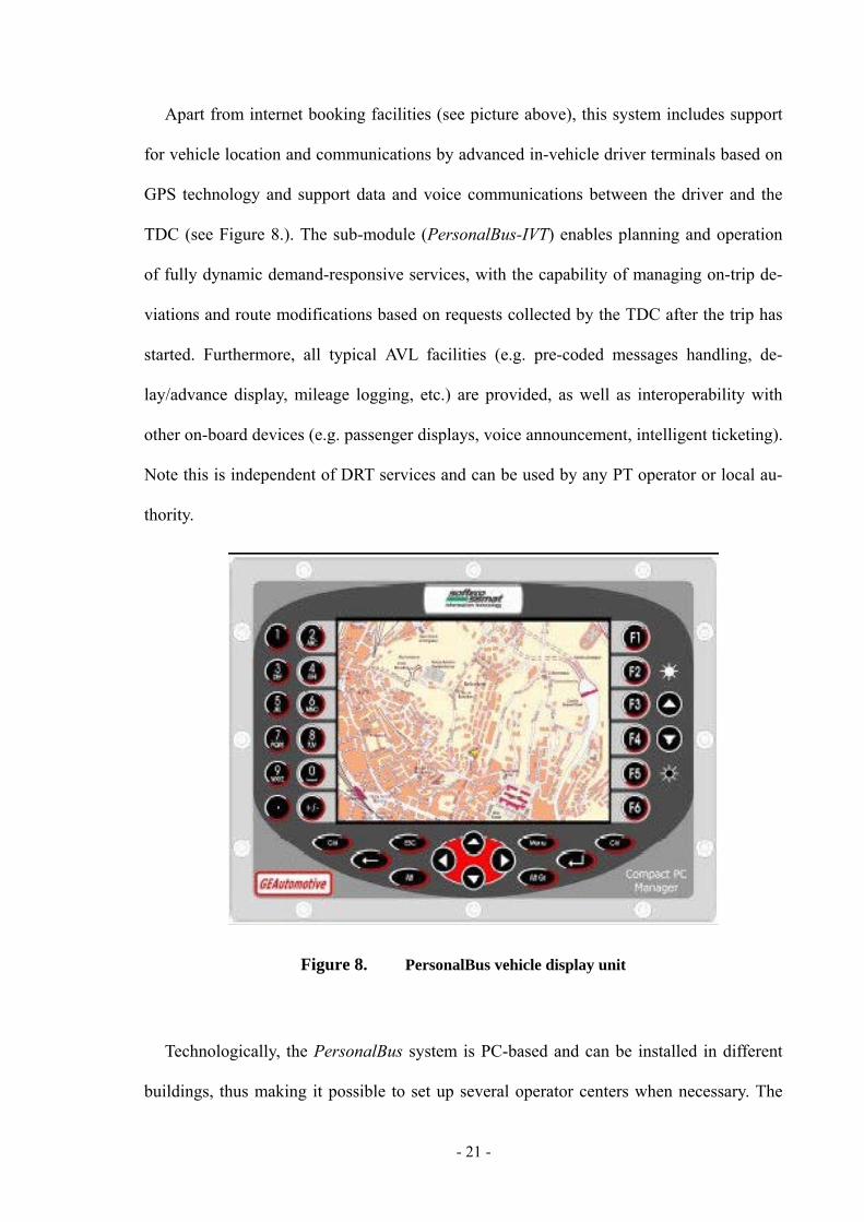
Apart from internet booking facilities (see picture above), this system includes support

for vehicle location and communications by advanced in-vehicle driver terminals based on

GPS technology and support data and voice communications between the driver and the

TDC (see Figure 8.). The sub-module (PersonalBus-IVT) enables planning and operation

of fully dynamic demand-responsive services, with the capability of managing on-trip de-

viations and route modifications based on requests collected by the TDC after the trip has

started. Furthermore, all typical AVL facilities (e.g. pre-coded messages handling, de-

lay/advance display, mileage logging, etc.) are provided, as well as interoperability with

other on-board devices (e.g. passenger displays, voice announcement, intelligent ticketing).

Note this is independent of DRT services and can be used by any PT operator or local au-

thority.

Figure 8. PersonalBus vehicle display unit

Technologically, the PersonalBus system is PC-based and can be installed in different

buildings, thus making it possible to set up several operator centers when necessary. The

- 22 -

basic hardware platform consists of a stand-alone PC that has been especially equipped to

guarantee satisfactory performance. The basic software platform consists of a Microsoft

Windows© NT/2000/XP operative environment. As with MobiRouter, the main data ar-

chive is based on an Oracle relational database. Geographic area maps are managed by a

MapInfo© GIS graphic tool, which is able to support any graphic format.

More information can be found on the PersonalBus website at

http://www.personalbus.it/.

2.2.3 LITRES-2

This work is done in Australia which seeks to develop technology that can meet the

needs of scheduling new forms of public transport such as demand responsive transport.

LITRES-2 is a R&D activity concerned with the simulation and scheduling of public trans-

port services. The first LITRES simulator was developed in 1993-94 and was applied in

planning studies for Canberra, Sydney and Perth. The most recent version, called LITRES-

2 (1996-97), handles multi-leg journeys and makes a clear distinction between simulation

and scheduling modules, with the scheduler designed for stand-alone use in real-time ap-

plications (TDC application). The LITRES-2 software provides a fine-grained simulation

capability for use in urban public transport planning. According to the developers, the

software is well suited to the investigation of initiatives and scenarios, including combina-

tions of conventional service (e.g. bus, rail and single-hire taxi) with novel modes, such as

demand-responsive and zone-based bus services. In the longer term, LITRES-2 is intended

as the kernel for traveler-information and fleet-scheduling systems.

LITRES-2 can handle the following transport modes:

· Conventional timetabled, pre-scheduled modes: bus, light rail, train, ferry.

- 23 -

· Medium-volume demand-responsive modes: "Taxi-Transit" and "Personal public

transport", which typically use vehicles intermediate in size between buses and taxis (e.g.

"maxi-taxis"). Such services probably are most valuable where demand is low or spatially

diffused (e.g. zone-based service in suburban areas late at night), and as feeders to main

bus and rail routes.

· Single and multiple hire taxis. Multiple-hire taxis differ from conventional taxis in that

more than one group of passengers can travel together. Services of this kind may be pro-

vided commercially, or under a cooperative car-pooling arrangement.

The system provides a detailed representation of travel behavior and service provision.

It comprises a simulator and a scheduler. Demand is specified by means of origin-

destination and source-sink models. The simulator disaggregates these models to generate

a time ordered stream of travel-requests. The methods used here allow for the overlaying of

a wide variety of spatial, temporal and socio-economic patterns of travel demand. Travel

requests are passed from the simulator to the scheduler. The scheduler’s journey-planning

module seeks to implement each request as a journey comprising one or more legs – possi-

bly including walking – so as to minimize travelers' generalized costs. The scheduler also

arranges bookings for journeys that involve the use of dynamically scheduled modes (e.g.

taxis). A central scheduler is needed to respond to prospective passengers' inquiries and

requests for travel, and to deploy vehicles efficiently. LITRES-2 includes embedded mod-

ules for two critical types of tasks in this respect:

1. The L2sched module controls the deployment of a fleet of demand-responsive pas-

senger vehicles. Functions include dynamic booking, scheduling, dispatching and routing.

Heuristic techniques are used, with the objective (broadly speaking) of minimizing vehicle

operating costs. This module has potential application as a real-time scheduling system for

a fleet of passenger vehicles, or for local delivery or courier services.

- 24 -

2. The L2jplan module emulates the decision-making processes of prospective passen-

gers. This involves minimizing for each passenger the generalized cost of travel (i.e. fares

plus the value the traveler attributes to his own time). A journey-plan produced by L2jplan

may comprise several legs, covered by walking, conventional modes (e.g. bus or train), or

demand-responsive services (e.g. taxi or smart-shuttle). L2jplan has potential application

as a component of a real-time information or booking-management service.

The scheduler has a graphical interface which can display travel requests that have been

processed so far (Figure 9), a journey plan for the current travel request (Figure 10), and

Figure 9. LITRES-2 scheduler: travel requests

- 25 -

Figure 10. LITRES-2 scheduler: journey plan for the current travel request

current itinerary for each vehicle. Note that L2sched is designed for use in conjunction

with radio-based dispatching systems and (optionally) with location-finding technologies

such as GPS. The operating modes that can be handled by L2sched include traditional

phone booked or "step-in" service; multiple hiring; and "smart shuttle" services working

nominally to timetables but run on demand. Thus the fleet managed by L2sched may be

- 26 -

restricted to "blue ribbon" taxis, but it may also offer a variety of lower-priced multiple-

hire services. Other possibilities include cooperative dial-a-ride arrangements, and special

services for the elderly and disabled.

L2sched plans passenger services as far ahead in time as possible. For instance, if a

booking is made six hours in advance, the passenger is immediately allocated to a vehicle

on a tentative basis. This provides scope for optimization, and helps to ensure reliability of

service. It is also consistent with a yield-management approach which would reward "early

booking" passengers with reduced fare rates. The optimization techniques used in L2sched

are designed to maximize the efficiency of fleet deployment over time (efficiency is typi-

cally defined in terms of minimizing total travel time or distance, or maximising the

number of passengers carried). Work allocations and routing plans can be revised in re-

sponse to events as they occur in real time (e.g. vehicle breakdowns), and to changes in the

spatial and temporal patterns of demand.

Detailed information about the road network is used, when planning fleet deployment

and routing plans for vehicles. This information includes provision for fluctuation of travel

speeds on the network over the course of the day. It is assumed that the dispatching tech-

nology provides information about current location when passengers are picked up and set

down. LITRES-2 has been used in planning transport services for the Gold Coast area of

Queensland, Australia. More information on the methodology can be found in [12] and

[13], and more general background information is available at

http://www.cmis.csiro.au/its/projects/litres2.htm.

- 27 -

2.2.4 SAMPO

The municipality of Tuusula, population 30,000, is located 25km north of the Helsinki

Metropolitan area. Tuusula’ s DRT system has been tested and implemented as part of a

regional partnership comprising three municipalities of the Keski-Uusimaa region. The to-

tal regional population is 99,000. Transport services in the region are delivered by private

taxi services, numerous bus operators (private and public), public transport services includ-

ing minibuses for mobility impaired and rail connections to Helsinki. The addition of the

DRT system has enabled complete geographical coverage of public transportation.

The Tuusula DRT system studied was an EU DG13 supported project called SAMPO

(System for Advanced Management for Public Transport Operations) [14]. The objective

of SAMPO was to set up and test DRT systems in Tuusula and other European cities in

Belgium, Italy and Sweden. The project ran between 1996 and 1997 and was continued

during 1998 and 1999 under the SAMPLUS project (System for Advanced Management for

Public Transport Operations). SAMPLUS focused on further evaluation of the SAMPO test

sites. The technology development is continued focusing on producing an affordable intel-

ligent in vehicle terminal (IVT).

The objective of DRT system is to fill geographical gaps in the existing public trans-

port services. The Finnish model is based on "open for all” principles, guaranteeing equal

access to public transport. DRT systems optimize the transport of special needs groups

such as the elderly or disabled who are not able to access public transport. It also enables

collective transport for example between airports and hotels and for tourist transportation.

It can also be used for enhancing, replacing or establishing flexible public transport in low-

density rural areas. DRT builds on the existing transportation network, integrating services

with regular public transport and encourages full utilization and non-competitive services

- 28 -

with existing public transport services. DRT aggregates demand and operates on multimo-

dal principles.

A relatively simple technical platform is used to deliver DRT systems. A central dis-

patch centre has a computer with DRT based software and can be operated by a single

person (for small to medium sized systems) or scaled up as necessary. Users call the travel

dispatch centre (TDC) to book single trips or to arrange scheduled trips - at least three

hours in advance. The SAMPO system provides fixed timetables and pre-ordered pick-up

and drop-off destinations. The centre recommends the best alternatives combining bus and

taxi services. The transportation fleet, which includes buses, minibuses and taxis, has GSM

based communication devices to receive passenger and route information. The SAMPO

DRT management system (see Figure 11.) combines the resources of multiple municipali-

ties through a shared travel dispatch centre.

The DRT system in Tuusula provides an excellent ‘test bed’ to evaluate the crosscutting

themes. Results from the DRT system are briefly highlighted below. DRT meets the lack of

public transport in rural areas providing solutions for school services, shopping trips, food

and goods transport, feeding services for fixed bus services, hospital transport and the eld-

erly and disabled. The DRT system is socially inclusive. Rural residents normally

accustomed to limited public transport services benefit from a flexible and timely system

overcoming barriers such as a lack of private transport or access to public services. Special

user groups receive door-to-door services non-existent prior to DRT. This greatly increases

mobility, access to public services and provides a significant increase to quality of life.

DRT provides a solution to battle the increasing costs in special transport services. DRT

systems are not necessarily the cheapest solution compared with urban public transport

however, it has been shown that, municipalities including Tuusula, have reduced the cost

- 29 -

of servicing rural areas to an annual decrease of 2-3% compared with an annual increase of

15%, including set-up costs.

Figure 11. SAMPO DRT management system

2.2.5 Project LT: DRT

LT: DRT has been developed and marketed by Logical Transport (LT) [15], a passenger

transport software company based in Portsmouth. In the company’s own words, “LT: DRT

can manage every aspect of the DRT operation from the initial booking of a travel request;

scheduling and monitoring of current commitments through to invoicing and driver bill-

ing.” The LT: DRT package includes mapping, GPS, driver communication, web booking

and real-time scheduling across the Internet.

The package specification includes:

- 30 -

· Fast telephone booking: The booking screen recalls customers’ popular journeys and

personal information to assist in quickly recording travel requests. Bookings can be classed

as one-offs or repeating bookings and can be automatically priced according to pre-defined

tax structures.

· Internet bookings: The internet booking facility can be used to streamline the booking

process and affect considerable savings on call-centre operating costs. Online customers

can create and review their travel requests at any time and receive activity reports of past,

current and future travel commitments.

· Visual Diary Scheduler: A visual representation of operations in advance over any time

scale is provided (see Figure 12 for a screenshot of the scheduler). LT: DRT is claimed to

be extremely flexible in that it enables a ‘mix and match’ approach to operations, i.e. part

of the fleet can be engaged in DRT operations, at the same time as other vehicles can be

dedicated to other activities such as excursion or contract services.

Figure 12. LT: DRT scheduler with visual representation of operations

- 31 -

· Real-time control centre: The software monitors and actions bookings that are waiting

to be performed, currently being undertaken and those that are complete. It allocates book-

ings to the operator’s fleet or third parties and controls progress through a specified ‘event

lifecycle’. The drivers’ shifts can be monitored to ensure that bookings are not allocated to

drivers that would put them beyond specified daily driving hours. Color and countdown

timings to reflect status and priority of each booking are displayed onscreen.

· GIS mapping: Integrated street level mapping down to premise level is available to

view all travel commitments and driver routes. The system can be configured to search for

shortest or quickest routes and can model differing traffic conditions at different times of

day, e.g. evening rush hours. Known trouble spots can be identified and avoided.

· Driver communication and positioning information: Using the latest PDAs with inte-

grated mobile phone capability (GPRS etc) help maintain full two-way data

communication with drivers. These computer devices can provide destination details and

pickup information and drivers in turn can communicate current position using GPS and

confirm status of the current travel request.

· Invoice administration and management reporting: Automated invoicing and reporting

of completed work for both cash and account clients. A variety of invoice printing styles

can be incorporated, including breakdown by cost centre or by individual accounts. Jobs

can be tagged as requiring supervisor review before being approved for invoicing in this

fashion you can assure that all job costing information has been correctly entered before an

invoice is raised. Production of sub-contractor self-billing and reconciliation reports are

available with an export file facility compatible with Sage Accounting software. Operators

are able to build a complete history of all transactions in line with financial periods.

- 32 -

The software has been designed and developed for Microsoft Windows and Microsoft

Internet Server. It will run on the following Window platforms: 95/98/NT/XP/2000. A

powerful server is needed to successfully run the central application. LT: DRT has so far

been used by Vodafone Ltd as an extension of their intranet and SMS based car share sys-

tem. More information is available at http://www.logicaltransport.com/drt/index.html.

2.3 Modeling Method for Urban Transport Simulation

Software modeling and simulation of urban transport systems, it had a hard position

during the 1970s [16]. Though relevant at the time, the field of geographic modeling and

simulation was revived by numerous advances in the related areas of research. Break-

throughs in the understanding of cities transport in general, as well as developments in

mathematics and computer science, have enabled new approaches in urban transport mod-

eling. In fact, the rise of the object-orientation paradigm in computer science provides both

an insightful way for modeling and simulation, as well as a useful technique for software

implementation.

2.3.1 Cellular Automata

Cellular automata (CA) [17] are presently the most popular modeling concept in urban

geography domain. Cellular automata are standard automata, but the input is defined in a

cellular context. In CA, each cell represents an automaton that is neighboring another

automaton in a grid of cells. There are different ways how neighborhood may be defined in

CA. The most popular approaches are the five-cell von Neumann neighborhood and the

nine-cell Moore neighborhood.

- 33 -

The definition of a CA is:

A ~ (S, T, R)

Here, R denotes the cellular neighborhood of A, therefore defining the boundaries of

input I. Changes of set S are again expressed through transport rules, virtually every possi-

ble discrete spatial process may be translated into transition rules for CA. Although cells

are stationary in CA, information can be propagated, depending on the implemented

neighborhood as stated above. In geographic modeling, CA is particularly popular for rep-

resenting areas with varying land use as cellular units.

2.3.2 Geo-simulation

Geo-simulation is concerned with the design and construction of spatial models, with a

focus on urban areas. These models are useful for exploring ideas and hypotheses about the

inner works of the complex spatial systems that these models represent. Geo-simulation

achieves that through object-oriented simulation software, which is then applied to real

world scenarios within a spatial context. It employs spatially related automata as a basic

concept for modeling. GIS and remote sensing databases serve as the predominant data

sources for geo-simulation systems.

The special feature of geo-simulation is its constituent elements. Geo-simulation fea-

tures a ‘bottom-up’ design, meaning that higher level entities such as census groupings are

a product of the dynamics of animated and unanimated objects at the lowest level of mod-

eling. These high-level entities may be considered emergent, in such as these high levels

are significantly richer in characteristics compared to the atomic objects that compound

them.

- 34 -

2.3.3 Optimal Multi-graph Simulation

The class of vehicle routing problems has drawn many researchers and industrial practi-

tioners’ attention during the last decades. These problems involve the optimization of

freight or passenger transportation activities. They are generally treated via the representa-

tion of the road network as a weighted complete graph, constructed as follows. The vertex

set is the set of origin or destination points. Arcs represent shortest paths between pairs of

vertices. Several attributes can be defined for one arc (travel time, travel cost . . . ), but the

shortest path implied by this arc is computed according to one single criterion, generally

travel time. Consequently, some alternative paths proposing a different compromise be-

tween these attributes are dismissed at once from the solution space. In the following, to

avoid any ambiguity between the paths of the new graph (working graph in the figure) and

the paths of the original road network, the latter are called road-paths.

In [18], Thierry GARAIX represents the road network with a multi-graph, so that alter-

native routes are considered. A simple insertion algorithm is proposed and illustrated in the

context of an on-demand transportation system was developed. Computational experiments

on academic and realistic data underline the potential cost savings brought by the multi-

graph mode. Ideally, one arc will be added between two vertices for each Pareto optimal

road-path according to arc attributes in the road network. Any good road-path would then

be captured in the graph. Practically, one could prefer just to consider a reasonable set of

arcs between two vertices.

2.3.4 Multi-agent Based Transportation Simulation

In computer science, the multi-agent system (MAS) is a system comprising multiple

autonomous and intelligent agents, which are capable of perceiving their environment and

- 35 -

acting upon that environment to achieve their goals. The main applications of MAS at the

moment are problem solving, multi-agent simulation, construction of synthetic worlds and

collective robotics. According to their study, a good behavior is measured by how success-

fully the agent’s action to achieve its goal. In 2003, Russell and Norvig [19] give out four

factors involved in design a rational agent:

• The performance measure defining the success criterion;

• The agent’s prior knowledge of the environment;

• The available actions of the agent;

• The agent’s percept sequence to date.

The application of new multi-agent technologies to urban traffic information systems

has made it possible to create intelligent systems for traffic control and management: the

so-called Intelligent Traffic Systems (ITS) [20] or Advanced Traffic Management Systems

(ATMS). The basic task of ITS is to support road managers in traffic management tasks

[21].

Because urban traffic networks have interrupted traffic flow, they have to effectively

manage a high quantity of vehicles in many small road sections. On the other side, they

also have to deal with a non-interrupted flow and use traffic sensors for traffic data infor-

mation integration. These features make it difficult for real time traffic management. The

urban traffic simulators can be classified into two main kinds: macroscopic simulator and

microscopic simulators. Macroscopic simulators use mathematical models that describe the

flows of all vehicles. In microscopic simulator, each element is modeled separately, which

allow it to interact with other elements.

Multi-agent systems are an efficient tool for the basis of urban traffic simulator. Many

researchers have made studies on this subject. In [22], Patrick A. M. Ehlert and Leon J. M.

- 36 -

Rothkrantz designed driving agents, which can exhibit human-like behaviors ranging from

slow and careful to fast and aggressive driving behaviors. In [23], J. Miguel Leitao uses

autonomous and controllable agent to model both the traffic environment and the con-

trolled vehicles. And their scripting language is based in a well-known graphical language,

Grafcet. In [24], Joacbim Wahle and Michael Schreckenberg present and review a frame-

work for online simulations and predictions, which are based on the combination of real-

world traffic data and a multi-agent traffic flow model. Nagel [25] discusses several as-

pects in the design of intelligent agents such as: route generation, activity generation,

learning framework, route re-planning and private knowledge, while no transportation

simulation integrates all the aspects. Guidi-Polanco et al. [26] present a case study of a

passenger transport planning system, in which transportation agents are identified in two

layers: the internet layer for communicating with the external world, and the scheduling

layer for scheduling and assignment services.

2.3.5 Comparison

We can see that all of the three approaches described above can be used to implement

the urban transport simulation environment. Geo-simulation is too complex to be a good

option since it aims at the most realistic and detailed modeling possible today. Cellular

automata are not the first choice for modeling moving objects like vehicles, since CA are

static in nature. Certain similarities nevertheless arise, since the urban street network of the

simulation used here is a regular grid world. Optimal multi-graph simulation use the math-

ematic way to simulation, it is different to simulate large-scale real-time system behaviors.

A multi-agent system is an autonomous intelligent computer system, in which every

agent always has a certain level of intelligence. The level of an agent’s intelligence could

- 37 -

vary from having pre-determined roles and responsibilities to a learning entity. A multi-

agent system is an aggregate of agents, with the objective of decomposing a larger system

into several smaller agent systems in which they communicate and cooperate with one

other. Agent-based model can produce high-quality simulations for complex and large-

scale system behaviors like the urban traffic system. The multi-agent based simulation ap-

proach is the most suitable technique for urban transport domain, because clients and hosts

can be modeled as more or less independent entities with their own behavior. The level of

complexity can be adjusted to make this approach feasible, making multi-agent based

simulation the method chosen for this work. Hence, the application of multi-agent system

to model and simulate urban traffic systems is highly suitable and can be very efficient.

- 38 -

Chapter 3. Theoretical Foundation

The objective of this chapter is to provide necessary theoretical foundation informa-

tion to familiarize readers with the context of this thesis. The work begins with a definition

of multi-agent system. The next section discusses the capabilities and limitations of the

multi-agent based modeling and simulation technique, laying a basis for the present model-

ing efforts. The last section details theory of demand responsive transport to establish an

outlook in creating the model assumptions, methods and implementations.

3.1 Multi-agent System

3.1.1 Agent Definition

As is very common in the field of Artificial Intelligence, there is no standard defini-

tion of an agent. Instead, it seems that almost every major research and survey yields yet

another definition. For the sake of completeness, some of the definitions of agent are pre-

sented below.

An agent is:

“A computer system, situated in some environment, which is capable of flexible

autonomous action in order to meet its design objectives” [27].

Others define an agent as:

• “An agent is a computational entity which: acts on behalf of other entities in an

autonomous fashion, performs its actions with some level of pro-activity and/or

reactive-ness, and exhibits some level of the key attributes of learning, coopera-

tion and mobility” [28].

- 39 -

• “A system that independently handles parts of the problem based on small inde-

pendent knowledge bases” [29].

• “An autonomous entity that interacts with the environment, and adapts its state

and behavior based on interaction” [30].

An agent has the following characteristics:

• Autonomy: An agent has its own beliefs, plans and intentions and it can accept or re-

fuse a request.

• Interaction: An agent interacts with its environment. The agent can change the envi-

ronment via its actions and the environment can change the agent’s actions.

• Collaboration: An agent must be able to collaborate with other agents in order to

achieve a common goal.

• Learning: An agent must have the ability to learn, based on previous experience from

its interaction with the environment. (See Figure 13)

Figure 13. An Agent In Its Environment

- 40 -

It is important to note that some of the typical agents and agent architectures do not

fully have all of the proposed characteristics. Sometime agent’s architecture do not have

full collaboration and learning characteristics [31], while agents in behavior based architec-

tures do not “consciously” collaborate [32]. The proposed set of characteristics can be seen

as the result of evolution of the desired characteristics for an agent and represents the cur-

rent typical approach to agency. The prospects of having a standard definition of an agent

are as good as having a standard definition of an intelligent system.

Classification schemes of agents are not relatively explored by a same standard. Some

classification schemes are implicitly given in various agent surveys and some explicitly.

Normally the classification of agents based on agent reasoning model, agent key attributes

and agent paradigm origin. The following sections discuss classification based on agent

reasoning models.

Classification based on an agent’s reasoning method is not new. Despite the fact that

classification based on reasoning method is not new, there is still no consensus on the exact

naming of the two main paradigms that form the basis of this classification. The two main

paradigms that form reasoning method classification are symbolic and sub-symbolic para-

digms. Symbolic and sub-symbolic paradigms are respectively referred to as traditional

and connectionist, or deliberative and reactive paradigms. These are all different names for

the fundamental division between two different approaches in the field of AI.

According to reasoning method, agents can be classified into the following three dis-

tinctive groups:

• Symbolic Reasoning Agents, which utilize a traditional AI approach based on logic

calculus. Traditional AI approaches are exemplified in the majority of expert systems. The

- 41 -

main characteristic of a symbolic reasoning agent is that it relies on symbolic representa-

tion of the real-world. Symbolic reasoning agents usually have the following components:

• A symbolic model of the world usually represented in some form of rules such

as first-order predicate logic.

• A symbolic specification of the agent’s actions usually represented as a rule

with a condition for its triggering, which consists of an antecedent (a conjunc-

tion of Boolean conditions) and a consequent (or action).

• A reasoning algorithm is that plans the agent’s future actions. All reasoning re-

lated computations usually rely on inference rules, expressed in first order

predicate calculus [33].

• Sub-symbolic Reasoning Agents, which do not maintain a world model, or if they do,

a non-symbolic representation is used for a world model. Sub-symbolic agents are some-

times called reactive agents. The main objective of sub-symbolic reasoning agents is to

minimize the amount of predetermined behavior, and to create agents that exhibit intelli-

gent behavior based on the agent’s interaction with its environment. In other words,

intelligent behavior should emerge.

The main characteristics of such agents are that they do not maintain a symbolic model

of the world and usually do not communicate with other agents. The consequences are that

a sub-symbolic agent’s reasoning is based on interaction with the local environment. De-

spite the well-documented shortcomings of sub-symbolic agents, some of the sub-symbolic

agent implementations have achieved spectacular results, albeit in very specific domains.

Like traditional decomposition of a mobile robot control system is one of reactive agent

systems [34]. (See figure 14.)

- 42 -

Figure 14. Mobile Robot Control System

• Hybrid Reasoning Agents, which combine the characteristics of symbolic and sub-

symbolic agents. Shortcomings of both symbolic and sub-symbolic models have become

apparent fairly early. Various hybrid models were proposed that try to exploit the best of

both approaches such as Touring Machines [35] (See Figure 15). Most hybrid architectures

are layered architectures, where lower layers are simpler (reactive or behavioral) and upper

layers are more complex, providing symbolic reasoning capabilities, as well as mecha-

nisms for cooperation between various agents.

Figure 15. Touring Machines

Control Subsystem

Planning Layer

Reactive Layer

Perception

Subsystem Action

Subsystem

Modeling Layer

Sensor Input Action Output

- 43 -

3.1.2 Multi-agent Systems

3.1.2.1 Multi-agent systems Definition and Classification

A system that consists of multiple agents is called a Multi-Agent System (MAS). MAS

are a generalization of an agent system where the main advantages of agents can be further

exploited, namely an agent’s ability to execute both autonomously and in parallel. MAS

are ideally suited for problems that can be either executed in parallel or that can employ

multiple problem-solving methods. However, the advantage of a MAS approach to prob-

lem-solving and parallelism does come at a price: interaction problems between

autonomous agents exist, including cooperation (working towards a common goal), nego-

tiations (coming to an agreement) and coordination (avoiding harmful interactions between

agents).

3.1.2.1.1 MAS Definition

There are various definitions of MAS. MAS can be defined as a loosely-coupled net-

work of problem-solvers that work together to solve problems that are beyond the

individual capabilities or knowledge of each problem-solver [36]. Other authors keep the

definition much simpler: MAS can also be seen as a society of agents [37].

Wooldridge and Jennings propose a rather strict definition of MAS that is based on

MAS characteristics:

• Each agent has incomplete information or capabilities for solving the problem,

thus each agent has a limited viewpoint.

• There is no global system control.

• Data is decentralized.

- 44 -

• Computation is asynchronous.

Figure 16. Multi-agent Systems

MAS have some characteristics:

• Each agent has complete or incomplete information about the problem or capa-

bilities to solve the problem [38].

• There is no global rigid control system. However, there can be a global coordi-

nating system, such as a supervisor.

• A complete set of data can be partially or completely decentralized.

• Computations are executed in parallel. (See figure 16.)

3.1.2.1.2 MAS Classification

- 45 -

Like the classification schemes of agents, there is various classification schemes of

MAS are in existence [39]. Some of the presented classification schemes are generalized

versions of agent classification schemes, while others are based on properties applicable

only to MAS such as communication models.

Classification Based on Reasoning Module

MAS can be classified according to the reasoning module employed by the MAS. Using

such a classification scheme, MAS can be divided into three classes: symbolic MAS, sub-

sumption MAS and hybrid MAS. These classes are presented in chronological order of

appearance.

Symbolic MAS

Symbolic architectures were the earliest to emerge as MAS. This is hardly surprising if

it is taken into consideration that a significant contribution to the agent paradigm came

from AI planning research, which was a very active research area during the 1970s and

1980s. Symbolic MAS are based on premises of the “physical-symbol system hypothesis”.

In [40], Newell and Simon, defined a physical symbol system as a:

“Physically realizable set of physical entities (symbols) that can be combined to form

structures and which is capable of running processes that operate on those symbols accord-

ing to symbolically coded sets of instructions”.

The physical-symbol hypothesis then stipulates that a physical symbol system is capable

of general intelligent action. In [27], Wooldridge and Jennings define a symbolic architec-

ture as “the architecture that contains an explicitly represented, symbolic model of the

world, and in which decisions are made via logical (or at least pseudo-logical) reasoning,

- 46 -

based on pattern matching and symbolic manipulations”. Typically, a symbolic MAS is

based on a problem-solving method, such as STRIPS (Stanford Research Institute Problem

Solver) [41] that employs a symbolic, centralized model of the world. A symbolic MAS is

based on the cognitive science sense-think-act cycle. The sense-think-act cycle assumes

that an agent senses a change in the environment deliberates about the change in the envi-

ronment and decides on an optimal or nearly optimal course of action and, lastly, executes

an action which may have an effect on its environment. In theory this sounds very good but

there were problems when implemented in real world environments. In practice, problems

such as slowness of deliberation and accurate real-world modeling were experienced. Sys-

tems such as STRIPS and General Problem Solver (GPS) have performed extremely well

in virtual worlds, where the model of the world was static and accurately given [42].

Sub-symbolic MAS

Once the limitations of symbolic MAS became obvious and theoretically proven, in[31]

Brooks had some criticism. As a complete opposite to the symbolic approach, an approach

where knowledge is subsumed was proposed in the seminal work by Brooks. In this purely

reactive approach, knowledge is subsumed in condition-action pairs. Intelligence is treated

as a “side-effect” of an agent’s interaction with its environment. The subsumption architec-

ture employs no symbolic knowledge at all. Hence there is no model of the world. It

assumes that intelligent behaviors emerge from interaction between more primitive behav-

iors represented, essentially, as action-reaction pairs. The subsumption architecture has

been surprisingly successful, despite its apparent simplicity, but there are serious disadvan-

tages of this architecture. An obvious problem is that, because of the lack of a world

model, every agent decides on its actions based on information from its local environment.

- 47 -

Therefore, there is no coordination as such, actions are only locally optimal, and overall

behavior is not easily understood.

An additional problem is that there is no effective way for an agent to learn from ex-

perience, as there is no direct feedback loop from consequences to actions. By the 1990s it

was accepted that the subsumption architecture may be applicable to certain problem do-

mains, such as modeling of insect behavior, but it was not suited as a general architecture

[43]. An attempt to reconcile symbolic and sub-symbolic approaches resulted in the next

class of MAS, i.e. the hybrid MAS.

Hybrid MAS

Hybrid MAS is a result of trying to use the best of both worlds, i.e. symbolic and sub-

sumption MAS. Two main problems of the symbolic architecture, namely its slowness and

the problem of accurate world modeling were related to its interaction with its environ-

ment. Most of the strengths of the symbolic approach come from its deliberative and

planned approach to acting on stimuli from the environment. On the other hand, the main

strength of the sub-symbolic architecture stems from its efficient interaction with its envi-

ronment and the main weakness is the fact there is no efficient, goal-driven interaction

between agents. A typical hybrid system uses both symbolic and subsumed knowledge and

exploits the strengths of each approach.

Typically, a hybrid MAS is a layered system, where different layers use different

knowledge representations. The higher levels are based on symbolic knowledge reasoning,

while lower levels are usually implemented using a sub-symbolic approach. A layered

MAS exhibits symbolic planning and coordination, coupled with fast, efficient interaction

with the environment. An example of a hybrid MAS is Multiple Automata for Complex

- 48 -

Task Achievement (MACTA) [44] that utilizes a symbolic planner as a symbolic compo-

nent, while a sub-symbolic component is implemented using the Behavioral Synthesis

Architecture (BSA) [45].

Classification Based on Cooperation Level

With the appearance of MAS, the issue of avoiding negative interaction (or conflict) by

means of negotiation and the issue of cooperation by means of coordination became very

important. The potential for exhibiting negative interaction is due to the autonomy of

agents, who may have their own beliefs, desires and intentions that are not necessarily

shared between all agents. If agents’ intentions are conflicting, a conflict may arise be-

tween the agents in MAS. Classification of MAS based on the level of cooperation was

proposed in the late 80s [46]. The cooperation based classification scheme has been

adopted by other researchers [47]. According to level of cooperation between agents, MAS

can be divided into:

Cooperative Multi-Agent Systems

Cooperative MAS, historically the first to appear, have their background in early Dis-

tributed Artificial Intelligence (DAI). In cooperative MAS, the emphasis is not in

optimizing the performance of an individual agent, but that of the whole system. This class

of MAS roughly corresponds to symbolic MAS, as symbolic MAS often employ symbolic

representation and cooperation enabling techniques that rely on symbolic representation of

the world model. The consequence is that a global world model must be maintained. The

main focus of research in cooperative MAS is that of coordination between the agents.

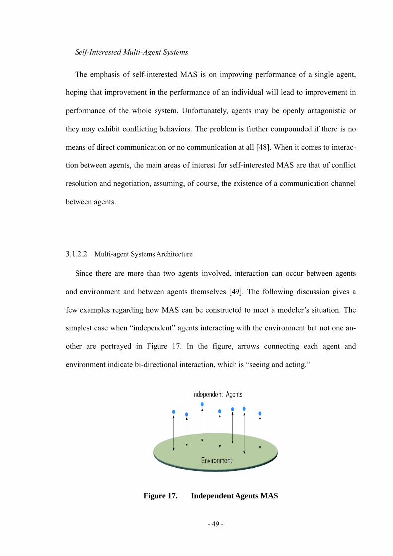
- 49 -

Self-Interested Multi-Agent Systems

The emphasis of self-interested MAS is on improving performance of a single agent,

hoping that improvement in the performance of an individual will lead to improvement in

performance of the whole system. Unfortunately, agents may be openly antagonistic or

they may exhibit conflicting behaviors. The problem is further compounded if there is no

means of direct communication or no communication at all [48]. When it comes to interac-

tion between agents, the main areas of interest for self-interested MAS are that of conflict

resolution and negotiation, assuming, of course, the existence of a communication channel

between agents.

3.1.2.2 Multi-agent Systems Architecture

Since there are more than two agents involved, interaction can occur between agents

and environment and between agents themselves [49]. The following discussion gives a

few examples regarding how MAS can be constructed to meet a modeler’s situation. The

simplest case when “independent” agents interacting with the environment but not one an-

other are portrayed in Figure 17. In the figure, arrows connecting each agent and

environment indicate bi-directional interaction, which is “seeing and acting.”

Figure 17. Independent Agents MAS

- 50 -

However, in general, there are many examples of agents who interacting with one an-

other. One famous example of this is flocking behavior of birds. Birds, when they fly

together, watch obstacles in their flight direction as well as adjacent neighbors to avoid

possible collision and to be inside of their group [50]. In this case, agents can communicate

with each other and act directly on other agents' states. The information layer, shown on

top of Figure 18, is introduced to present this mechanism.

Figure 18. MAS with Information Layer

An advanced MAS architecture can be constructed using multiple information layers.

Figure 19 shows a multi-agent system in which case agents interact with the environment

as usual but part of them collectively behaves as a group. The agents in the figure are di-

vided into two groups: group X and group Y. Agent Xn follows the rules, exchanges

information, and affects other members in its group who share the same kind of behavioral

patterns and rules through information layer X. Likewise, agents in group Y, which may

retrieve a different set of information from the environment and affect the environment in a

different way, do so with their own rules without (or with) consulting group X. Many hu-

- 51 -

man social behaviors follow this architecture. A representative example would be the stock

market where individual and institutional investors form different groups and act differ-

ently.

Figure 19. MAS with Multiple Groups

The last architecture of multi-agent configuration is that of organizational architecture,

shown in Figure 20. The best example can be found in military organization where the

general is the head and the order passes down from top all the way to the bottom level. The

lowest level agents, analogous to private soldiers or fighters, directly interact with the en-

emy and the environment around them. The agents X and Y in the intermediate level gather

information and report this, such as attrition, to the super agent. They can control the low-

est level agents with their own discretion as long as their goals obey the super agent's

instructions.

- 52 -

Figure 20. MAS with Hierarchical Organization

In fact, the modeler can construct virtually any form of agent-based model with the ap-

propriate architecture depending on the nature of the application problem. In next section,

we will introduce multi-agent based modeling (ABM) and simulation.

3.2 Multi-agent Based Modeling and Simulation

On the technical side, computer simulations can be classified along several dividing

lines. As every computer simulation involves some kind of dynamics, an important ques-

tion is how to represent time. Time can be represented either as a continuous real-valued

- 53 -

variable (within the limits of today’s inherently discrete computers) or can be regarded as a

sequence of discrete symbols. Another, perhaps more important, issue is that in time-based

systems or in continuous event simulations the system state changes continuously in time,

while in discrete event systems, changes are assumed to take place instantaneously, at spe-

cific points in time. These points are the ones when ‘events’ occur. It is also important to

decide how the simulation handles the passing of time. In time driven systems time is ad-

vanced in constant small steps, so that state changes occur evenly in time. Most

continuous-time simulations use this approach, making the time step of the simulation suf-

ficiently small, so that there are no perceivable transitions within the system between the

steps. In these systems, time usually has a ‘physical’ meaning, that is, the simulated time

value directly corresponds to that of the modeled system. On the other hand, event driven

simulations take the opposite approach. They determine when events occur, and advance

the time variable to that point [51]. Event driven simulation is more efficient in the sense

that it doesn’t iterate through time steps when nothing happens. On the other hand, time

driven simulation is more suited to human interaction (e.g., training simulations), as simu-

lated time is more realistic in this case [52].

3.2.1 Agent Based Simulation

Agent-based modeling and simulation is a new and specialized branch of computer

simulation that emerged as a methodology for studying complex systems. While agent-

based modeling is most commonly applied to the simulation of social processes, it has also

been used in a wide range of other fields, such as ecology, biology, anthropology, psychol-

ogy, and traffic & vehicle simulations [53]. Agent-based models are generally used to

perform highly abstract thought experiments [54].

- 54 -

The approach bears several names. In ecology, it is called individual-based modeling

(IBM), while some people call it multi-agent simulation [51] or multi-agent based simula-

tion (MABS). The most widely accepted name, however, remains agent-based modeling.

In principle, agent-based modeling (ABM) refers to the research methodology of construct-

ing models in a particular way, and agent-based simulation (ABS) is a particular way of

implementing simulations. However, almost all agent-based simulations are constructed

using the ABM methodology and vice versa. Therefore the two terms are often used inter-

changeably. In the following, wherever the meaning is clear from the context, I will adopt

this practice.

As mentioned before, agent-based modeling is a bottom-up approach that looks at what

happens when a diverse group of individuals interacts locally. Agent-based models consist

of agents and an environment (sometimes people call it: space or framework) . The agents

have states and behavioral rules. States can be fixed for the life span of the agent or can be

dynamic. The fixed states are often called parameters, while the dynamic ones variables.

The environment may be spatial (e.g., a rectangular grid), or non-spatial (e.g., an abstract

trading community).

Most importantly, interactions among agents take place in the environment component.

The adaptive and autonomous agent operates in the following manner: First, an agent sees

the world, and then it makes a decision that entails an action. The world is influenced,

however unimportantly, by the action. The same agent now senses a different world, and

updates its knowledge, which may then cause a different action or even shift its goal. Ac-

cumulated action of the agent produces an emergent behavior, which often renders a useful

insight to the real world even if a model itself is in a very simple form. (See Figure 21)

- 55 -

Figure 21. Concept of Agent-Based Modeling

Interactions among agents take place in the environment component. Interactions can be

direct, where an action immediately changes the state of a partner, or indirect, where an

action changes the environment, which, in turn, causes a partner’s state to change. In any

case, the embedded nature of agents implies that the type of interactions among the agents,

often referred to as the interaction topology, is an inherent and highly explicit part of the

model. Another important aspect is that the environment may be also active, having its own

behavior [55]. This allows for the development of models in which the agent population

co-evolves with the environment. (See Figure 22)

- 56 -

Figure 22. Interactions Among Agents

A simple formalization of these ideas, assuming a discrete-time system, is the following.

Let vector A denote the internal states of all agents. Similarly, vector E stands for envi-

ronmental states. Then, the abstract form of an agent-based model can be written as two

update functions:

A (t+1) =f (A (t), E (t))

E (t+1) = g (A (t), E (t))

When building agent-based models, the modeler has to define the cognitive and sensory

capabilities of the agents, and the actions they can carry out, together with a description of

the environment and its activities. Given this ‘compartmentalization’ ABM supports ‘struc-

ture preserving modeling’ of the simulated system. That is, there is a close match between

the entities of reality, the entities of the model, and the entities of the simulation software.

It is also a fundamentally important point of the methodology that agents interact without

the control of a central authority. Global patterns emerge from the bottom up, determined

- 57 -

not by a centralized authority but by local interactions among autonomous decision-

makers. [56]

After the rules for guiding an agent's actions and the relationships between the agent

and environment are established, a computational model that imitates the real world is

simulated. The observation and analysis should follow the simulation invoked by a user:

i.e., let them play and watch it. For this reason, agent-based modeling and simulation

(ABM/S) can be thought of as a scientific reasoning approach that complements deduction

and induction. In [57], Axelrod clearly explains this point as follows:

Like deduction, it starts with a set of explicit assumptions. But unlike deduction, it does

not prove theorems. Instead, an agent-based model generates simulated data that can be

analyzed inductively. Unlike typical induction, however, the simulated data come from a

rigorously specified set of rules rather than direct measurement of the real world. Whereas

the purpose of induction is to find patterns in data and that of deduction is to find conse-

quences of assumptions, the purpose of agent-based modeling is to aid intuition.

The major strength of ABM/S comes from the fact that it is a simple, versatile and

flexible method that is well suited for studies of complex non-linear systems. Agent-based

simulations can reveal both qualitative and quantitative properties of the real system, so

ABM/S can be used as a versatile laboratory to perform experiments to test nearly any kind

of imaginable hypotheses. ABM/S, however, does have a downside. For a highly realistic

model, large amounts of data input and computation may be needed. In [58], another issue

for ABM/S is that identifying the right, rules or behaviors that capture the real dynamics

can be a somewhat ad hoc process.

- 58 -

3.2.2 Application of Multi-agent Based Molding and Simulation

Although present applications of ABM/S have become very numerous, it was not until

mid 1980s that the concept of agent based modeling blossomed with the evolution of com-

puter technology. Additionally, as the amount of fundamental research on complex systems

grew, the use of agent-based modeling and simulations became more widespread. Below

lists a few applications of ABM/S found in the literature.

Natural Sciences

Ecology would be one of active application fields within the natural sciences. In [59],

Fishwick, Sanderson &Wolff presented modeling method for use in large-scale ecosystem,

focusing on the dynamics of species with the Florida Everglades. Hartvigsen & Levin [60]

developed an agent-based model of plant-herbivore interactions to test the interactive ef-

fects of explicit space and co-evolution on population and community dynamics.

ABM/S technique is also naturally adapted to the study of animals or plants. In [61],

Sumpter presented a mathematical study of determining the relationship between the local

interactions of individuals in a population and the global dynamical behavior of that popu-

lation in the context of honey bee behavior, using a variety of modeling techniques

including ABM. Scheffer et al. [62] tried to model behaviors of fish population with their

super-individual approach, an ABM technique which aims to enhance computational effi-

ciency. Deutschman et al. [63] carried out computational simulations of forest dynamics

using an individual-tree model of the forests of the northeastern United States.

Though not an obvious match, ABM/S has even found a fit in chemistry. McMullin &

Varela [64] applied ABM/S to the field of artificial chemistry and presented simulation re-

sults which exhibits spontaneous emergence and persistence of auto organization.

- 59 -

Social sciences

The nature of the social sciences is the study of the human aspects of the world. ABM/S

is a promising technique for social scientists in economics, political science, sociology and

psychology. Its development has revived old and raised new questions regarding the dy-

namics of complex human society. In economics, a new branch of economics-called agent-

based computational economics (ACE)-is fledging with increasing attention recently. Prac-

tical applications of ACE can be abundantly found. Basu, Pryor, Quint & Arnold [65] have

built a micro-analytic model, called Aspen, to simulate the U.S. economy. Raberto et al.

[66] carried out an agent-based simulation to look at a behavior of a virtual financial mar-

ket through a realistic trading mechanism for price formation. An excellent survey paper is

given by Tesfatsion [67] regarding this blooming field. Other social sciences have actively

adopted ABM/S as well. Chakrabarti [68] is building an ABM to provide a connection be-

tween theoretical study of corruption developing micro models of individual acts and

empirical study of corruption at the country level. McPhail [69] discussed collective ac-

tions of people in large assembling and dispersal such as crowds, mobs and

demonstrations. Helbing, Farkas & Vicsek [70] also performed a simulation study on ag-

gregate behavior of individuals in a panic situation. Benenson & Omer [71] are doing an

interesting research to demonstrate the dynamics of urban residential distribution of Arab

and Jewish people in a few Israeli cities. Merelo, Prieto & Rivas [72] attempt to forecast

the effects of mass media advertising using ABM/S.

3.2.3 Advantages and Disadvantages

The most often claimed advantages of agent-based modeling and simulation can be

summarized as follows.

- 60 -

• Bottom-up, generative method.

• Represents the environment and the interaction topology explicitly.

• Handle heterogeneous (diverse) and dynamic populations.

According to Ross Hammond “traditional models – to permit mathematical solution –

must often use either homogenous actors, or so-called representative agents.” This is no

longer necessary in ABM. Similarly, dynamic population can easily lead to the intractabil-

ity of traditional models. [73]

• Enforces realistic computational abilities for the agents.

Traditional social sciences, especially neoclassical economics, make very strong as-

sumptions about rationality. Individuals are assumed to have perfect information, and

infinite time and computational power to make complicated decisions. Agent-based mod-

els, for comparison, directly enforce the implementation of the agent’s decision-making

processes, therefore limiting their computational ability. Thus most ABMs use bounded

rational agents that have only “local, limited information, and limited ability and time to

process that information”. Some writers go that far as making agent simplicity a methodo-

logical requirement for ABM [53]. Others argue that agent simplicity is only due to the

relative novelty of the approach and due to the lack of better tools. It is important to see,

however, that the computational bounds imposed by ABM are there independent of the

model’s sophistication in depicting agent cognition. Moreover, “… often the main concern

is not to model general cognitive capability, but to investigate the consequences of

bounded rationality.”

• ABM is arguably capable of modeling emergent actors and institutions.

Holland and Miller suggest that artificial agents can be used as ‘subjects’ in pilot studies

to identify potential areas for human experiments. Participatory agent-based simulation, a

- 61 -

new area even within the field of agent-based simulation, implements this idea by provid-

ing tools to mix human subjects with artificial agents within the same computational

experiment [74].

Technically, agent-based simulations are most often discrete-time, discrete event, event

driven simulations, although exceptions exist to each of these properties. Generally they

are built in an object-oriented programming language, although special purpose agent pro-

gramming languages also exist.

One serious disadvantage of ABM:

• Generally slower and require more computers resource.

When compared to more aggregate modeling methods, is due to its bottom-up approach.

Implementing behavioral rules for each low-level individual may be more demanding than

calculating the dynamics of aggregate global variables. Therefore, agent-based simulations

are generally slower and require more powerful computers than, e.g., the simulations of the

more traditional systems dynamics approach.

In summarize, agent-based modeling and simulation is a bottom-up approach to under-

standing complex systems. It encodes attributes and behaviors at the individual component

or microscopic level of the system. It is thus a powerful complement to top-down modeling

approach, particularly because it allows for the implications of assumptions that are neces-

sarily made in top-down analysis. Whereas agent-based models can be made arbitrarily

realistic by capturing the processes, mechanisms or architectures that drive individual

components, they can also be made quite abstract in an attempt to understand .the essence

of the problem. As pointed out by Bonabeau [75], ABM/S is particularly useful for model-

ing of flows, markets, organizations, and diffusion in which system behaviors change due

- 62 -

to learning or adaptation. He further states that ABM/S can bring significant benefits when

1) the interactions are complex, nonlinear or discontinuous, 2) an agent is spatially explicit,

3) agents are heterogeneous, 4) the topology of the interactions is heterogeneous and com-

plex, and 5) agents exhibit learning and adaptation behavior. However, unlike other

approaches based on mathematical formalism, there can be an element of subjectivity in

constructing and testing an agent-based model. Also, the simulations of ABM/S are poten-

tially very intensive from a computational aspect.

3.3 Theory of Demand Responsive Transport

In this section, we will introduce demand responsive transport from economic point

view. Transportation demand analysis are discussed in this section, stemming from the lit-

erature spread including Kanafani [76], McCarthy [77], Labbé et al. [78] and Noland [79],

among others. The discussion begins with basic foundations of neoclassical economics.

3.3.1 Neoclassical Economic Theory

For planning transportation facilities, it is necessary to forecast how much they will be

used. In order to price them rationally and determine the best operating policies, it is nec-

essary to know how users respond to prices and service characteristics. In order to evaluate

whether a project is worthwhile at all, it is necessary to have a measure of the benefits it

produces. All these requirements are in the province of neoclassical economic analysis.

Neoclassical economic theory postulates that human beings are self-interested and

highly rational when it comes to making decisions about economic activity. In other words,

human beings select the choices that offer them the best possible advantage, given the cir-

- 63 -

cumstances they face. Circumstances involve a wide variety of factors: the prices of goods

and services, and the constraints on the decisions that may make such as income, regula-

tions and technology limitations. Another premise is that our greed is non-satiable; the

more, the better, always. Based on these postulations, neoclassical economists regard that

any individual has a capability of comparing alternatives.

The demand transport decisions are often envisioned as a sequence, typically starting

with residential and job locations, then vehicle ownership, then other aspects. This se-

quence is in decreasing order of the time span over which the decision can be changed

easily. However, it does not imply a sequential decision procedure whereby one decision is

made without regard to its implications for later decisions. Rather, each decision is affected

by others and so can be fully understood only as part of a simultaneous choice process. A

given study may isolate just a few of these decisions for tractability; it is then all the more

important to remember, in interpreting results, that other decisions are lurking in the back-

ground.

In addition, travel is a derived demand, usually undertaken to facilitate a spatially varied

set of activities such as work, recreation, shopping, and home life. This observation links

the study of travel demand to studies of labor supply, firms’ choices of technologies, and

urban development. It also calls attention to an increasingly common form of travel: the

linking together of several trip purposes into one integrated itinerary or tour, a process

known as trip chaining.

For more formal analysis, the approach most similar to standard economic analysis of

consumer demand is an aggregate one. The demand for some portion of the travel market

is explained as a function of variables that describes the product or its consumers. For ex-

ample, total transit demand in a city might be related to the amounts of residential and

industrial development, the average transit fare, the costs of alternative modes, some sim-

- 64 -

ple measures of service quality, and average income. Because behavior cannot be predicted

precisely, an “error term” is added to represent behavior that, to the researcher at least, ap-

pears random. Thus a demand function might be represented as:

x = f (Z) +ε

Where: x is the quantity demanded, Z is a vector of values of all the relevant character-

istics of the good and its potential consumers, f ( ) is some mathematical function that

depend on which domain apply, and ε is the random error term. Statistical data on x and Z

can be used to estimate the function f and the probability distribution of ε.

It is possible to estimate f using non-parametric methods that impose no prior assump-

tions about its shape. More commonly, f is specified to be a particular functional form with

parameters whose values are to be determined from statistical data. For example, f might

be specified as a general quadratic function:

Where: Zk is one of the characteristics included in vector Z, Zl is a factor that possibly

affects the extent the effect of Zk upon f, and the β parameters are to be estimated empiri-

cally. This is an example of an equation that is linear in parameters. To see why, define

variables z0≡1, z1k=Zk, z2k=Zk2, and z3kl=ZkZl, for all values of k and l. Combining all these

variables into a single vector z and all the corresponding parameters into a single vector β,

we can write as:

x = β′z +ε

Where the prime on β indicates transposition (changing it from a column vector to a row

vector); thus β'z is the inner product between β and z. So this equation is known as a re-

gression of x on z. When it is linear in β, as in this example, one can very easily estimate

the unknown parameters. Indeed, we chose this example to illustrate that even a quite

- 65 -

complex relationship between x and Z can often be represented as a linear regression. The

most common way of estimating the unknown parameters is ordinary least squares, which

the value of β is found that minimizes the sum of squared residuals for a set of observa-

tions labeled n =1,…, N:

Where now we have indexed each observed data point (xn, zn) by its observation label n.

Ordinary least squares has particularly nice properties when the random error ε is assumed

to have a normal (bell-shaped) distribution. However it is quite possible to estimate regres-

sion models non-linear functional forms or with other error distributions.

The non-random part of the demand equation is often based on an explicit theory of

consumer choice. Such a theory is not necessary in order to specify and estimate a demand

function, but it may help by suggesting likely functional forms for f and it is useful for in-

terpreting the results. The most common such theory postulates that a consumer or group

of consumers maximizes a utility function, u(x, X); this function expresses preferences over

the quantities of the good x under consideration and of other goods represented by the vec-

tor X. The consumer is limited by a budget constraint, expressed in terms of the price p of x

and a price vector P consisting of prices of all the other goods X. Mathematically, then,

consumption is determined as a solution to the following constrained maximization prob-

lem:

Where y is income and again the prime on P transposes it so that P′X is an inner prod-

uct, expressing the cost of consuming all the goods in vector X. Denoting the solution to it

by vector (x*, X*), we note that it depends on prices and income:

- 66 -

But if we knew, or were willing to postulate, a form for the function u, and if we could

solve the maximization problem, we would know the form of the demand function except

for its random term.

For the demand functions, when we derived in this way, can be used to define a very

useful quantity. We simply substitute them into the utility function to see how much utility

can be achieved with a given set of prices and income. The result is known as the indirect

utility function, often written as V:

V (p, P, y) = u(x * (p, P, y), X * (p, P, y))

The indirect utility function has a property known as Roy’s identity:

Where it is understood that all quantities in x * depend on p, P, and y. We will make use

of the indirect utility function and Roy’s identity when we discuss disaggregate demand

analysis. For cleanness, our notation for demand functions will omit the asterisks in x* and

X*.

The demand functions (x*, X*) were defined as resulting from an individual consumer’s

optimization. An aggregate demand function can simply be derived from individuals’ de-

mands by summing quantities demanded over consumers. Under some quite restrictive

conditions, the resulting aggregate demand function may look as if it could have resulted

from optimization by a single “representative” consumer, which can be convenient in

analyses. Specifically, a necessary and sufficient condition for this to be true is that indi-

- 67 -

viduals’ indirect utility functions take the “Gorman form”, meaning that for an individual i

it can be written as Vi (p, P, y) = ai (p, P) + b (p, P) · yi, where the ai-term can vary across

consumers. This condition is satisfied for several utility functions commonly used for theo-

retical analysis.

3.3.2 Derivation of Transportation Demand

Suppose a hypothetical situation that transportation and all other goods are given by a

commodity bundle (t, x) which contains t units of transportation (T) and x units of all other

goods (X). As shown previously, an indifference curve can be generated that gives the con-

sumer the same level of utility. However, this does not necessarily mean the consumer has

no limitations in selecting any alternatives on the iso-utility curve. The consumer always

has constraints under which she/he seeks to maximize the utility. In microeconomic de-

mand theory, it is common to consider the monetary budget constraints since it is usually

the most important.

Now consider a case that a consumer who has the monetary budget B1. Then the com-

bined expense for purchasing T and X should not exceed the budget B1. The quantities t and

x that a consumer can afford is dictated by:

PT* t + PX * X ≤B1

Where: PT and PX are the prices of T and X. Any pair (t, x) comprises the feasible

choice set (or opportunity set) for a consumer. A consumer's final alternative can be found

by solving a simple optimization problem as follows:

Maximize U (t, x), or minimize -U (t, x)

- 68 -

Subject to: PT * t +PX * X ≤ B1

A commodity pair is a solution to this equation, illustrated in Figure 23(a) where a1 =

(t1, x1) is located on the tangent point of the budget line and the utility curve U1. Suppose

the consumer's income increases. This causes a rightward parallel shift in the budget line

since the amount of budget will also increase to B2 (> B1). The expansion of feasible choice

set poses a new constraint and the consumer's choice moves to a2 = (t2, x2) which offers

increased utility to the consumer, as shown in Figure 23(b).

Figure 23. Income Effect on the Consumer's Choice

The effect of changes in price of T or X, all else being constant, results in expansion or

contraction of a consumer's choice set. Consider the transportation price PT used to be p2

but there is an incident that leads to higher transportation prices. The price is p3 now, so the

t-intercept of the budget line shift leftwards, which brings contraction of the feasible choice

set. Then, a consumer's selection point also changes with lower amount of transportation

with potentially less impact on all other goods as shown in Figure 24(a). If this process is

repeated with different prices, a general description of relationship between transportation

price PT and transportation demand t can be obtained, shown in Figure 24(b).

- 69 -

Figure 24. Generation of Transportation Demand

Suppose PT is replaced with a vector_p . The vector

_p can be thought of as a list of gen-

eralized prices which describes `the amount of resistance' a consumer feels such as the

actual price and transportation time of T. These components of _p have a negative impact

on t, but one can think of some components that have a positive impact, for example, the

consumer's budget and the price of other competing product X. In economics, the elasticity

is frequently used to measure the consumer's responsiveness of the demand function t

(_p ) with respect to p, a component of

_p . It is defined as the ratio of percent change in p to

percent change in t. In mathematical way, the elasticity can be expressed as:

A nice feature of the elasticity is facilitating comparisons of the demand to any of the af-

fecting variables, since tpε is dimensionless and independent of the units for t and p. One

limitation of the concept of the elasticity is that it cannot accommodate non-cardinal vari-

- 70 -

ables. (e.g. high/medium/low, building a new road, technology infusion, etc.) Another

weakness is that it is not applicable if more than one variable are simultaneously changed.

In order to deal with these situations, the perturbation and the sensitivity are defined next.

Perturbation (P): The change in system's state v, from v0 to v1, denoted by vp 1,0 . If the

change involves only a single variable in cardinal number, the perturbation can also refer to

the amount of the difference of that variable with respect to its reference (or baseline) value

v0, i.e., 0

011,0 v

vvpv −=

Sensitivity (S): The difference of system's dependent variable η with respect to its ref-

erence value η0 brought by the perturbation vp 1,0 i.e.,

These definitions are very generic and will be used in later chapters. It is very important

to keep track of state v0 and state v1 when the sensitivity is compared to other sensitivity.

The elasticity simply equals to the ratio of the sensitivity to the perturbation as v1 ap-

proaches v0, the reference or baseline state.

While this equation is mathematically rigorous in regard of Equation tpε , it is not gener-

ally required (or possible) to take the limit in practice; instead small perturbation-on the

order of a few percent-is adequate enough. The elasticity without taking the limit is fre-

quently used, called the arc elasticity e, and it can be calculated through the following

equation:

- 71 -

Which has an advantage since it gives the same value regardless of perturbation se-

quence. Still, it is very important to keep track of v1 and especially the reference state v0. It

is meaningless to compare which dependent variable's effect is significant when the base-

line state is not the same.

3.3.3 Trip Distribution Models

The transportation activity is essentially to link people or goods that are spatially sepa-

rated. Consequently, the study of transportation demand should be implemented with

distribution of trips in origins and destinations. The first step to study trip distribution is to

divide physical space under investigation into mutually exclusive zones or locations. Then,

the trip distribution can be conveniently specified in a matrix form. If tij(k) indicates the

number of trips during a given time period k between origin location i and destination loca-

tion j, an n-by-n matrix T(k) = [tij(k)] can be constructed where n is the number of

locations. This matrix is often called trip table, trip distribution matrix or origin-destination

(O-D) matrix. In general, a typical O-D matrix is not symmetric and shown in Figure 25.

Figure 25. The O-D Matrix

- 72 -

From the O-D matrix, trip production and attraction of each location can be easily ob-

tained. The trip production of i, Pi (k) is the sum of row i representing the total number of

trips originating from location i. The sum of column j, Aj(k) is the total number of trips des-

tined to location j and is called the trip attraction of j. The grand total D(k) of the O-D

matrix, called total trip demand, represents the total number of trips across all locations.

The following summarizes the characteristics of the O-D matrix.

∑ j ti j(k) = Pi (k)

∑ i ti j (k) = A j (k)

∑ i Pi (k) = ∑ j A j (k) = ∑ i,j ti j (k) = D(k)

Creating and estimating a reliable O-D matrix forms a crucial basis for the study of the

transportation demand analysis. The simplest approach is to utilize the concept of growth

factors.

When a priori knowledge is available, growth factor models are most frequently used,

though some variations can be found. They basically attempt to predict the future demand

by multiplying observed trips by some scaling factor. The simplest model has a constant

growth factor for all tij(k) but in practice each element of the O-D matrix has a correspond-

ing growth factor, that is:

ti j (k+1) = g ij (k) * tij (k)

Where (k+1) is an index for indicating the next time period after time period k. The

concept of the Hadamard product [80] is useful in converting equation tij (k+1) into a ma-

trix equation, and introduced in the followings.

Hadamard Product : Let Mm,n denote the set of m-by-n matrices. The Hamadard product

of A = [aij]∈Mm,n and B = [bij] ∈ Mm,n is AoB ≡[aij *bij]∈Mm,n.

- 73 -

Hadamard Exponent: Let A = [aij] ∈Mm,n then the Hadamard exponent of the matrix A

in the order of m is denoted by A[m] and its component is obtained by calculating aij m.

Using the above definitions, Equation ti j (k+1) is equivalent to the following matrix

equation: T (k+1) = G (k) o T (k) where G (k) = [gij (k)]. Further, if G (k) is a constant ma-

trix with respect to k, the trip distribution after k periods can be easily computed with the

initial trip distribution T (0) as follows:

As seen, growth factor models are a very intuitive and simple approach for estimating

the O-D matrix. They are particularly useful for forecasting of near-term demands espe-

cially when a clear trend is identified in the past data. However, growth factor models do

not have the capability to account for changes in the system that in turn affects growth fac-

tors. Hence, various trip distribution models have been suggested to properly reflect the

effects of influencing variables into the O-D matrix. Kanafani [76] (1983) observes that

most of trip distribution models have a general form given as follows:

tij = µivjCij

Where µi and vj are functions of the socioeconomic characteristics of locations i and j,

respectively; and Cij is a general function representing the impedance to travel between i

and j. He further suggests that trip distribution models can be classified into three major

categories: demand models, choice models, and spatial interaction models. The first two

groups are rooted in utility theory while the last one is derived from analogies of physical

laws.

The most basic approach to modeling trip distribution is to construct a demand model

for trips between an origin and a destination. This model can be an individual or aggregate

- 74 -

function, depending on the information available for calibration. It is derived by using the

utility maximization principle discussed previously. Assume a utility function for an indi-

vidual living location i is represented as follows: U =U (xi1, xi2,…..; xin) where xij is the

number of trips from the origin i to destination j. Associated with these trips, total travel

cost are given by C = ∑j cij xij where cij is a unit travel cost from i to j. Maximizing U under

the constraint C can be solved by constructing a Lagrangian: L =U-λC where λ is a Lagran-

gian multiplier. Then derivatives of L mush vanish so that U has optima:

∂U ⁄ ∂xij = λcij, for all j

Which states that constant is the ratio of the marginal utility to the trip cost for all loca-

tions. In order to solve the Lagrangian equations, however, an analytic form for U should

be given. A common utility function to use is a linear combination of the constant elasticity

utility functions [81] which can be expressed as:

ij

jijij xU ρα∑=

Where αij and ρij are parameters and 0 < ρij < 1 to satisfy the law of diminishing mar-

ginal utility. Substitution this into the Lagrange equations makes xij to be solved for. The

result is:

From which a general structure can be observed as follows:

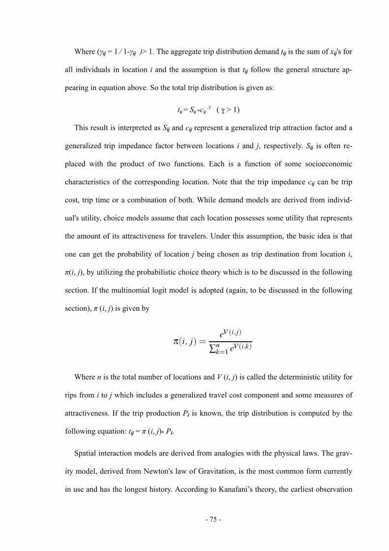
- 75 -

Where (γij = 1 ⁄ 1-γij )> 1. The aggregate trip distribution demand tij is the sum of xij's for

all individuals in location i and the assumption is that tij follow the general structure ap-

pearing in equation above. So the total trip distribution is given as:

tij = Sij *cij -γ ( γ > 1)

This result is interpreted as Sij and cij represent a generalized trip attraction factor and a

generalized trip impedance factor between locations i and j, respectively. Sij is often re-

placed with the product of two functions. Each is a function of some socioeconomic

characteristics of the corresponding location. Note that the trip impedance cij can be trip

cost, trip time or a combination of both. While demand models are derived from individ-

ual's utility, choice models assume that each location possesses some utility that represents

the amount of its attractiveness for travelers. Under this assumption, the basic idea is that

one can get the probability of location j being chosen as trip destination from location i,

π(i, j), by utilizing the probabilistic choice theory which is to be discussed in the following

section. If the multinomial logit model is adopted (again, to be discussed in the following

section), π (i, j) is given by

Where n is the total number of locations and V (i, j) is called the deterministic utility for

rips from i to j which includes a generalized travel cost component and some measures of

attractiveness. If the trip production Pi is known, the trip distribution is computed by the

following equation: tij = π (i, j)* Pi.

Spatial interaction models are derived from analogies with the physical laws. The grav-

ity model, derived from Newton's law of Gravitation, is the most common form currently

in use and has the longest history. According to Kanafani’s theory, the earliest observation

- 76 -

that the magnitude of population movements between cites is similar to the gravitational

pull between masses was suggested by Ravenstein in 1885. The basic structure is in line

with the law as follows:

Where µi and nj indicates a function of characteristics of origin i and destination j such

as Pi and Aj, respectively and cij is representing impedance between i and j. Keeping strict

gravitational framework would take kij = k and cijγ= dij 2 where dij represents distance be-

tween locations i and j.

Another approach based on physical analogy is the entropy model introduced by Wilson

[82]. In this approach, the entropy of the O-D matrix T is given by

This has the lowest value 1, when all trips are aggregated on a particular cell in the OD

matrix. Just like physical cases, this pseudo entropy is maximized in order to achieve sys-

tem's equilibrium. Consider that the optimization problem is subject to the following

constraints: ∑ j tij = Pi, ∑ j tij = = Aj, and ∑ j tij =B. The first two constraints and the last

constraint mandates that the total transportation cost expended is limited to a budget B.

Formulating a Lagrangian equation and differentiating with respect to tij result in the fol-

lowing expression.

t ij = kij Pi Aj e-λcij

Where: kij and λ are parameters for model calibration. For more details about derivation,

refer to [83].

- 77 -

Different trip distribution models discussed so far are subject to diverse model assump-

tions and so have generated a wide variety of modified forms. Despite the variety, all

models have some same objectives. For example, we think that every good model should

be properly responsive to socioeconomic factors and other transportation related condi-

tions.

We would like use multi-agent planning approach to solve DRT problem. In our multi-

agent based simulation approach for DRT system: multi-layer hybrid planning model, which

uses planning domain based agents planning framework to coordinate the plans of demand

responsive transport systems. The system offers trip solutions to client’s requests, at the

same time use minimal number of taxi, from socioeconomic view the system also proposes

good solutions.

We will introduce our approach and model in next chapters.

- 78 -

Chapter 4. Multi-agent Planning

Many situations involve decision making, like our situation: demand transportation

tasks to be carried out, use minimum resource (vehicles…) for the DRT systems. Often the

problem structure is the same: the world is in a certain state, but managers or directors

would like it to be in another state. The problem of how to get from the current state of the

world through a sequence of actions (possibly concurrent) to the desired goal state is a

planning problem. Ideally, to solve such planning problems, people would like to have a

general planning-problem solver. Since it turned out to be inherently impossible to design

an algorithm with a reasonable time complexity that can solve all planning problems cor-

rectly, several simplifications of this problem have been made in the past, eventually

leading to what may be called ‘the classical planning problem’. Although not all realistic

problems can be modeled and solved as such a classical planning problem, they can help to

solve more complex problems.

We would like to use multi-agent planning approach to solve our problem. So in this

chapter, at first we will give an overview of planning techniques for this classical planning

problem. Then we review current approaches to single agent planning. This is done for two

reasons: to give the reader a basic understanding of the range of approaches, and to identify

the approaches that are may be suitable for extension to multiple agents.

Then we discuss relevant approaches to multi-agent planning. Multi-agent planning ap-

proaches can roughly be divided into two categories: those that explicitly deal with the

interaction of plans of agents and those that use some kind of market or economy to ensure

that no conflicts occur and help agents take advantage of positive interactions. Each agent

in such a multi-agent system has to solve some form of planning problem. The most stud-

ied and accepted ‘basic’ planning problem is the classical planning problem.

- 79 -

In next chapter, we will present our multi-agent based simulation approach for DRT sys-

tem: multi-layer hybrid planning model, which uses planning domain based agents planning

framework to coordinate the plans of demand responsive transport systems.

4.1 Classical Planning Problem

The classical planning problem can be defined as follows [84]:

• A description of the known part of the initial state of the world in a formal language,

usually propositional logic, denoted by I.

• A description of the goal (i.e., a set of goal states) in a formal language, denoted by G.

• A description of the possible (atomic) actions that can be performed, modeled as state

transformation functions.

Determine a plan, i.e., a sequence of actions that transform each of the states fitting the

initial configuration of the world to one of the goal states. The formal language that was

used for STRIPS [41] is common to most classical planning frameworks.

4.2 Single Agent Planning

Planning is a process of search. The planning agent is given a set of input information

such as the current state of the environment, a set of actions that may be performed and a

set of goals to achieve, and searches through possible sequences of actions until it finds a

suitable solution plan. This is a hard problem as the space of possible sequences can be

very large. Successful planning approaches involve an informed systematic search through

the possibilities until a solution plan is found, or until the agent is reasonably sure that no

- 80 -

solution exists (either the search space has been exhausted or a timeout interval has passed

without a solution being found).

This section reviews current approaches to single agent planning in an attempt to iden-

tify approaches suitable for adaptation to multiple agents. We describe the refinement

planning paradigm, which is not a specific approach but a framework in which many plan-

ning algorithms can be expressed and compared using common concepts and terminology.

Refinement planning is used throughout the rest of this thesis in the discussion of single

and multi agent planning mechanisms and algorithms alike. Then we describe various re-

finement planning mechanisms that might be used as a basis for multi agent planning, and

alternative local search planning approaches that do not fit into the refinement framework.

4.2.1 Refinement Planning

Planning can be formulated as a search through possible candidate action sequences to

find a solution that achieves the desired result. The refinement planning paradigm [85] in-

volves starting with a state representing the set of all possible action sequences and

gradually shrinking it to a single solution sequence. Refinement planning maintains an

open list of sets of candidates that have yet to be considered, allowing the agent to perform

a sound, complete, systematic search of “candidate space”, but limiting its applicability to

environments that are static during planning. By contrast, local search planning does not

provide soundness and completeness guarantees, but is more suited to dynamic environ-

ments.

- 81 -

Partial plans

Sets of candidate action sequences are specified using sets of constraints, called partial

plans. A partial plan simultaneously represents all the action sequences that are consistent

with its constraints. As constraints are added to the partial plan, so the set of candidate se-

quences decreases in size. The planner is finished when it has a partial plan in which all

candidates are solutions.

Consider, for example, a planning formalism in which actions may be inserted at any

point into a totally ordered list. The empty list represents all possible candidate sequences

as no commitment has been made to any actions or orderings. The list (go to shops, go to

cinema….) represents all candidate sequences in which the shops and cinema are visited,

in that order but not necessarily immediately after one another.

If the planning algorithm only allowed the addition of actions to the beginning or end of

the list, the same list would represent all candidate sequences in which the shops and cin-

ema are visited consecutively. Thus, the set of sequences represented by a partial plan is

dependent on the plan representation used and the set of planning operators available to the

agent. In practice, depending on the partial plan representation chosen, it may not always

be possible to represent the desired set of candidates at a particular stage of refinement us-

ing a single partial plan. For example, the list based representation from the example above

is only capable of representing totally ordered action sequences, so it cannot be used to

represent the plan “visit the shops before or after cinema”. Strictly speaking, refinement

planning operates on sets of partial plans that represent all necessary candidates.

Refinement planning algorithm

- 82 -

A generalized deterministic refinement planning algorithm is shown in Figure 26 and

graphically in Figure 27. The algorithm takes an initial partial plan, representing a large set

of candidate sequences, as input, and progressively refines it to produce a solution plan in

which only solution sequences remain. The solution plan in Figure 27 contains a single so-

lution sequence, but in practice several solutions can be represented in a single plan. In

iteration, the planning agent chooses a feature of the plan to improve, called a refinement

(line 10). A refinement can be many things including the removal of a flaw, the extension

of the plan by an action, or the making of a specific decision.

1 function bfs (initial ) → solution: 2 create empty open list 3 (open_list← push (initial , open_list) 4 while ¬empty(open_list): 5 (plan, open_list)← pop(open_list) 6 if is_solution(plan): 7 solution←plan 8 return 9 else: 10 ref ← pick_refinement(plan) (not a backtracking point) 11 open_list← push (plans (ref), open_list) 12 solution ← failure

Figure 26. Generalized algorithm for refinement planning

- 83 -

Figure 27. Refinement search in a space of candidate plans (adapted from Na-

rayek, 2002)

There may be more than one way of performing a given refinement. For example, there

may be more than one way of resolving a particular problem or performing a particular

task. Each of these ways is embodied in a planning operator (or sequence of operators)

leading to a valid partial plan. The agent chooses an appropriate operator and applies it to

the plan (line 11). Each successive operator fills in more constraints, and the process con-

tinues until a solution plan is found (line 6) or no more valid plans can be generated.

Consider, for example, an agent trying to produce a list of up to five letters, chosen from

the set {A, B, C, D, E} representing any dictionary word. The complete set of candidate

sequences can be generated by appending different combinations of letters to the end of an

empty list. The agent starts with an empty letter sequence and adds it to its open list (line

3). In iteration, the agent removes a partial sequence from the list and checks if it is a dic-

tionary word (line 6). If so, the agent returns the word as a solution. Otherwise, the agent

applies the append_letter refinement (line 10), generating all possible sequences resulting

- 84 -

from appending a single letter and adding all sequences of five letters or less back to the

open list (line 11).

In most planning algorithms an agent will be able to perform more than one type of re-

finement. In the example above the agent could have been given a preprend_letter

refinement as well as an append_letter one. A single refinement r0 is picked per partial plan

p0 visited during search. When r0 is applied to p0, it should output a set of plans P1 that,

between them, represent the complete set of candidate sequences of p0. If each of the

members of P1 contains some kind of definite flaw, the agent can signal failure immedi-

ately: it does not have to backtrack and try an alternative refinement of p0. For example,

there are no words in the English language that contain three or more identical consecutive

vowels: if the agent in the example above were to come across the partial sequence

“AAA”, it could discard it immediately without considering the derivatives “AAAA”,

“AAAB”, “AAAC” and so on.

Planning approaches: The refinement planning algorithm can be altered to resemble

almost any modern planning algorithm by changing one or more of the following features,

referred to collectively as a planning approach.

Plan representation: This is the type of data structure used to represent the plan, in-

cluding features such as temporal and resource models. The choice of representation

affects the sets of candidates that can be stored in a single partial plan. This affects how

many plans the agent has to produce to cover all possible ways of performing a refinement,

and consequently the number of plans that need to be visited per refinement in the worst

case.

- 85 -

Refinements and operators: The refinements available to the planner affect the effi-

ciency, completeness and branching properties of the algorithm. They affect the ability of

the planner to directly tackle specific flaws in a plan, minimize the production of redundant

plans, and so on.

Choice of refinement: The choice of refinement (pick refinement function, line 10) has

a large effect on the performance of the algorithm. Strategies such as least commitment

[86] and the identification of separable sub-problems [87] require the agent to identify re-

finements early on in planning that shape search later on. In particular, refinement choice

affects:

• How quickly sets of invalid action sequences can be pruned from the search

space;

• The ability of an agent to commit to plan features in a multi agent environment,

for the benefit of fellow agents;

• The redundancy in plans visited during planning;

• Whether second or third parties need to be contracted to help resolve conflicts in

multi agent problems.

Heuristics: Heuristics may be used to help pick the refinements that will produce the

maximum benefit later on, and to choose the order in which to investigate partial plans

once they have been generated.

Solution and failure test functions: The solution function (line 6) is used to identify

complete or partial solutions when they arise. In some cases this can be a complex prob-

lem, as it will not always be obvious whether some or all of the candidate action sequences

in a partial plan are solutions. Other functions may also be made available to identify un-

- 86 -

resolvable flaws in some partial plans and prune the corresponding branches of search (as

with the three vowel example above).

Search algorithm: The push and pop functions can be implemented in various ways to

produce different search algorithms. Stack like functions produce depth first search, queue

like functions produce breadth first search and so on. The most common form of search in

planning is A* and best first (heuristic only A*) search, which treat the open list as a prior-

ity queue sorted by a heuristic measure of plan quality. Depending on the nature of the

planning problem, however, other algorithms may prove more useful. Search algorithms

are discussed in more detail by Russell and Norvig [88].

The aspects of planning listed above are collectively referred to in this thesis as a plan-

ning approach. The same aspects minus the planning algorithm are collectively referred to

as a planning mechanism. Thus:

Approach = mechanism + algorithm

While we concern with multi agent planning rather than single agent planning, a limited

discussion of the basic approaches to single agent planning is required. Refinement based

planning approaches can be divided into two categories: those that search in the space of

states of the environment that may be visited by performing actions, and those that search

in the space of possible plans. These paradigms, called state space and plan space planning

respectively, are briefly introduced in the following sections. In next sections, we will dis-

cuss the STRIPS (Stanford Research Institute Problem Solver) [41] action representation

that is common to many planning algorithms, state space approaches, the two basic types

of plan space planners: least commitment and hierarchical planners. Finally, Section 4.2.6

discusses a class of local search planners that do not fit into the refinement planning

framework.

- 87 -

4.2.2 STRIPS (Stanford Research Institute Problem Solver)

The first planner was the General Problem Solver (GPS) of Newell and Simon [89].

GPS could solve various problems, including planning and theorem proving, through the

iterative application of logical rules. Work on planners has since focused on more specific

formalisms better suited to the production of efficient planning algorithms. GPS was suc-

ceeded by STRIPS [41], the most commonly known planning system. The major

contribution of STRIPS was a compact action representation that is still used by many cur-

rent planners. A STRIPS action consists of three parts: a description, a precondition

formula and a set of effects. For example the action of traveling between neighboring

towns might be represented as follows:

Action: travel (? a, ? b)

Preconditions: at (? a) ^ road (? a, ? b)

Effects: {at (? b), ¬at (? a)}

where travel is the name of the action, ?a and ?b are variable arguments representing

towns and at (?x ) and road(?x , ?y) are Boolean valued state literals. In English this trans-

lates as:

Preconditions: To travel from ?a to ?b there must be a road from ?a to ?b and the trav-

eler must be at ?a.

Effects: Once the traveler has moved, he is no longer at ?a: he is at ?b instead.

Planning variables: Variables are used to specify actions that can be applied to more

than one object. They allow a partial specification of the arguments of an action. Actions

- 88 -

and literals are referred to as grounded if all their arguments refer to objects in the world

and lifted if they contain one or more variables. Variables are bound to world objects when

an agent decides to commit to a specific action during planning.

Variables in preconditions are existentially quantified, referring to a single object in the

world. Variables in effects must appear in the action description or preconditions. This al-

lows the planning agent to analyze the predicted state of the world at the time when the

action is due to start and bind variables accordingly to produce the desired effects.

Plans: A complete STRIPS plan is a totally ordered sequence of grounded actions. The

following conditions hold for a plan:

• The plan is valid if the preconditions of each action match subsets of the world

state immediately before the action is executed (taking into account the effects

of previous actions).

• The plan is a solution to a problem if goals of the problem match a subset of the

world state immediately after the last action in the plan is executed.

Extensions to STRIPS representation: The STRIPS action and plan representation are

extremely simple. They lack many features that are considered convenient or necessary to

represent “real world” applications. Examples include:

1. Universal quantification of variables in preconditions or effects;

2. “Conditional action effects” that depend on world state at the time of execution;

3. Decomposition of actions into smaller parts, or aggregation of actions into “macro ac-

tions” (for example for learning);

4. Negative or disjunctive preconditions;

5. Typed planning variables and world objects;

- 89 -

6. Actions with duration and/or delayed effects;

7. A quantitative temporal model;

8. Metric or non-Boolean world state;

9. Actions with uncertain or unpredictable effects;

10. Sensing actions that reveal world state;

11. Conditional branching depending on world state or action effects;

12. Looping.

Some of these features are a convenience, reducing the work needed to encode planning

problems but not actually adding any representational power. Other features represent

types of problem and plan that simply cannot be represented using the STRIPS formalism.

Universal quantification and conditional action effects were first addressed by the Ac-

tion Description Language (ADL) [90] and later by the well known Planning Domain

Definition Language (PDDL) [91]. PDDL, in its various incarnations, has also provided

support for many of the other features above, although noticeably not looping.

While many of the features above are useful for solving real world problems, only a few

are strictly necessary for dealing with multiple agents. The most important features in this

regard are a sufficiently expressive model of interactions and relationships between con-

current actions [92]. Early work by Georgeff [93] on process models helped laid the

groundwork for understanding in this area. Support for sensing actions or uncertainty are

also potentially useful if agents have severely limited knowledge of the world, although

less so if agents are able to exchange information before plan execution to get a complete

picture of world state. Other features such as universal quantification and conditional ef-

- 90 -

fects reduce potential maintenance on plans in dynamic worlds where external changes

may cause action effects to change.

4.2.3 State Space Planning

The first category of refinement planners, state space planners, includes STRIPS itself.

State space planning involves searching in the space of possible world states. Reachable

states are determined by simulating the effects of actions. State space planners are given

three initial inputs:

1. A set of symbols O representing objects in the world and a complete description of

the initial world state I. World state is specified as a set of literals defined on tuples of ele-

ments from O.

2. The goal state G, also specified as a set of literals. G does not have to be a complete

description of world state; unspecified literals are assumed to be unimportant and are ig-

nored when checking for goal states.

3. A set of actions A, in STRIPS or some equivalent representation.

They proceed in one of two ways:

• Forward chaining planners start at the initial world state and search forward in

time. Actions are added to the end of the plan, which is assumed to be totally or-

dered, until a state is reached that matches the goal state.

• Regression planners do a similar search starting at the goal state and working

backward towards the initial conditions.

Despite the intuitiveness of state space planning, the space of reachable world states is

vast and for many years no good techniques were known for guiding algorithms to solu-

- 91 -

tions [94]. This meant that for a long time state space planners were only able to handle

small problems and plan space planning dominated. Recent work on planning graphs [95]

has revived state space planning by providing a compact way of simultaneously represent-

ing alternative orderings of actions.

Planning graphs: Planning graphs are a compact plan representation that forms the ba-

sis of some of the fastest current planning techniques. In figure 28, a planning graph is a

relaxed representation of possible action sequences and reachable world states. It consists

of interleaving layers of propositions representing possible future states and possible

choices of actions. Layers 1 and 2 represent possible state and action choices at time 1,

layers 3 and 4 represent possible state and action choices at time 2 and so on.

The graph is constructed with a forward chaining search, in iteration extending it by one

unit of time (or two layers). Because layers represent possible future states, individual lay-

ers can contain nodes that would be mutually exclusive in a single possible world. Mutex

arcs are used to denote pairs of mutually exclusive state and action nodes in each layer. At

iteration the graph is searched for possible plan sequences if the goal state is a non-mutex

subset of the final state layer. Plan retrieval is done with a backward search that makes

heavy use of mutex information in the planning graph. More recent extensions to planning

graphs handle many extra features, including universal quantification and conditional ef-

fects, exploitation of symmetry, automatic type identification and exploitation, uncertainty

and sensing actions [96], metric resources, quantitative time and durative actions with de-

layed effects [97]. Many of the fastest modern planners [98] plan in state space and use

planning graphs either directly or as the basis of heuristics [99].

- 92 -

Figure 28. Planning Graph of a Simple Route Planning Problem.

4.2.4 The Least Commitment Planning

Least commitment planning introduced by Marr [100], has been used in many fields of

AI, including computer vision, planning and theorem proving. It involves deferring deci-

sions about the temporal orderings and variable bindings until they are required to resolve

conflicts in the partial plan. Least commitment allows the planner to be flexible about parts

of its plan until it has enough information to work out the best possible course of action.

While many of the fastest current planning algorithms are based on state space planning, it

is this flexibility that makes plan space planning, including least commitment planning,

interesting from a multi agent perspective. Least commitment planners are often also re-

ferred to as “partial order planners” or “Partial Order Causal Link (POCL) planners”. The

following is a simplified version of the description of UCPOP provided by Penberthy and

Weld [101]:

A partial plan p is a tuple < A, T, B, L > where A is a set of actions, T is a set of temporal

constraints, B is a set of variable bindings and L is a set of causal links. The preconditions

and effects of an action a∈ A are referred to as pre (a) and eff (a) respectively. Actions are

- 93 -

unordered and lifted by default; constraints are added to T and B where necessary to im-

pose temporal orderings, ground variables and remove conflicts. By changing the language

of implementation of T [102], a number of qualitative and quantities temporal models can

be implemented with varying complexity and expressiveness [103].

A causal link is a structure ai ⎯→⎯l aj where ai and aj are actions in A, ai is ordered be-

fore aj and l is an effect of ai and a precondition of aj. ai and aj are referred to as the

provider and consumer of the literal respectively. Causal links are added to the plan to pro-

tect preconditions, making sure they do not come under threat from actions with

conflicting effects.

Least commitment planners are given two initial inputs:

1. An initial plan p where:

• Ap contains two dummy actions: a0 and a∞, eff (a0) represents the initial state of the

world, pre (a1) represents the goal state, a0 is ordered before a∞, Bp is empty, Lp is empty.

2. A set of actions in STRIPS representation or some equivalent.

They proceed by iteratively selecting an action aj and unachieved precondition l∈pre

(aj) and trying to achieve it by making the following refinements to the plan:

• Adding a causal link ai ⎯→⎯l aj from an appropriate existing action ai;

• Adding a new action ai that may be used as a provider and a causal link ai ⎯→⎯l aj ;

• Removing a threat to an existing causal link ai ⎯→⎯l aj from an action ak with ¬l ∈

eff(ak) by adding appropriate constraints to T and/or B.

A valid solution is a plan with no unachieved preconditions and no threats to causal

links. Penberthy andWeld [101] built on early least commitment planners in 1992 such as

SNLP [104] and TWEAK [105] to produce UCPOP, the first least commitment planner to

- 94 -

handle ADL (conditional action effects and universal quantification). Since then they have

gone on to produce Zeno [106], one of the most expressive current plan space planners,

which is capable of handling domain features such as metric resources and durative actions

with delayed and continuous effects.

4.2.5 Hierarchical Task Network Planning

The earliest plan space planners did not search in the space of task orderings and causal

links, but rather in the space of decompositions of actions [107]. These early planners gave

rise to another form of plan space refinement planning: Hierarchical Task Network (HTN)

planning [108]. Like least commitment planning, hierarchical planning allows a certain

amount of flexibility during planning. It also allows agents to reason at varying levels of

abstraction, which could be useful for reducing communications overheads and limiting the

complexity of inter-agent coordination in multi agent planning.

HTN planners are similar to least commitment planners in that they search in the space

of partial plans and explicitly model temporal and variable binding constraints. However,

they are different in the way they search the space: by considering the possible decomposi-

tions of abstract tasks. Just as the “flat” planners above are based on the notions of actions,

goals and plans, HTN planners are based on notions of tasks, task networks and methods:

Tasks subsume actions and goals. Rather than planning to achieve a set of goals, an

agent plans to perform a set of tasks. There are two types of task: primitive tasks that can

be executed directly and abstract tasks that must be decomposed into smaller tasks during

planning.

- 95 -

Task networks are used to represent plans and sub-plans. A task network n is a tuple <

A, T, B > where A is a set of tasks, T is a set of temporal constraints on the members of A

and B is a set of variable binding constraints.

Methods represent ways of decomposing abstract tasks. A method m is a tuple < h, b >

where h is an abstract task and b is a task network representing a sub-plan that achieves the

desired effects of h.

HTN planners are given two initial inputs:

1. A non-empty initial plan p containing abstract and primitive tasks those need to be

performed.

2. A set of methods M providing ways of decomposing abstract tasks.

They proceed by iteratively selecting a task t ∈Ap and decomposing it using an applica-

ble method m∈M by substituting for t with bm. Primitive tasks have preconditions and

effects in the same way STRIPS actions do. Abstract tasks have no preconditions and ef-

fects per se, although new preconditions and effects may be introduced when an abstract

task is decomposed. A single abstract task may have more than one applicable method, so

relevant preconditions and effects are not always known in advance. Conflicts introduced

during decomposition are resolved as they are in least commitment planning by adding

temporal or variable binding constraints.

Most HTN planners search only in the space of task decompositions. This is limiting

because every combination of actions has to have been thought out in advance by the hu-

man designer of the method library. This is the major objection raised against HTN

planning by supporters of “flat” planning techniques, but it does not prevent HTN planners

being the most widely used planners in industry for two reasons:

- 96 -

1. HTN is an intuitive way of thinking about planning, and many planning systems in

industry are mixed initiative systems that interact with human operators as well as per-

forming automated search.

2. Human designers can encode problem specific knowledge into methods such that the

planner produces predictable plans in a timely fashion.

Consider, for example, a manufacturing scenario in which it is necessary for a particular

machine to produce a diagnostic report every time it is used. The specification of this con-

straint in a “flat” planning formalism would require the addition of state information and

action preconditions and effects to ensure that every time a use machine action is added to

a plan, a produce report action is also added. This is a non-trivial adjustment to the plan-

ning domain, and would add an extra layer of complexity to the problems given to the

planner. In HTN planning, however, the produce report task would simply need to be

added to the relevant method, and the planner would not need to do any extra processing to

ensure its use at the relevant points in the plan.

Recursive versus non-recursive domains: HTN planning problems can broadly be

classified into ones that contain recursive methods and ones that are not. A method m is

recursive if Bm contains a subtask, some part of which may be decomposed with m. Block-

sworld is a classic example of a recursive HTN domain:

In order to pick up block A, I have to make sure there is nothing on top of it. If there is a

block B on top of A, I must pick it up and place it on the table. In order to pick up block B

I have to make sure there is nothing on top of it. If there is a block C on top of B, I must

pick it up and place it on the table...

Conflict detection: HTN planners are prone to backtracking because preconditions and

effects are only added to the plan after tasks have been decomposed.

- 97 -

Consider, for example, an agent planning the preparation of an exotic meal as shown in

Figure 29. This is done in three decompositions: first, the agent chooses whether to prepare

a Chinese or an Indian meal, then it shops for the ingredients, and finally it cooks and eats

the meal. Chinese meals involve eating with chopsticks: if the agent doesn’t have any

chopsticks, it will be unable to find a suitable plan if it uses the prepare_chinese method. A

human would immediately recognize this and choose to make an Indian meal. An unin-

formed HTN agent, however, may choose prepare_chinese and make all sorts of decisions

about which shops to visit, which ingredients to buy, and how long to cook the noodles,

before realizing that the chopstick requirement cannot be satisfied.

Figure 29. Example of HTN Planning

A number of planning systems use control strategies to guide search and stop the plan-

ner making “poor” choices of decomposition: The Task Formalism (TF) of the early HTN

planner [107] allows the domain designer to specify several types of information about

methods. For example, a high level effect of a method m specifies an effect that the body

of m is designed to achieve. An unsupervised condition of m specifies a precondition of a

descendant of m in the decomposition hierarchy that no other descendant is able to

achieve. These pieces of information can help the planner prune inappropriate choices of

- 98 -

method, but can affect soundness and completeness. For example, a high level effect of a

method m may affect the soundness of a planner if one or more decompositions and lin-

earization of m do not have an appropriate concrete effect.

Similarly, SHOP [109] and SHOP-2 [110] allow human domain designers to annotate

methods with the preconditions for situations in which they should be applied: a human

designer could add a requires chopsticks precondition to the the prepare chinese method to

prevent it being used when chopsticks are not available. This requires the planner to totally

order tasks and decompose them in the order they will be executed, so that the complete

world state is known at the beginning of each abstract task. SHOP requires method bodies

to be totally ordered. SHOP-2 relaxes this requirement, creating a totally ordered plan from

partially ordered methods. Tsuneto et al. [111] present a technique for automatically com-

puting external conditions of methods from the decomposition hierarchy, by looking at the

possible interactions between the descendant tasks of a method. External conditions serve

the same purpose as Tate’s unsupervised conditions, but because they are automatically

calculated rather than designed by a human, they can be shown to never affect soundness

or completeness. Similar work by Clement and Durfee [112] use summary information de-

rived from methods and subtasks to detect possible conflicts directly between abstract tasks

in non-recursive propositional HTN domains. They use this information both as a heuristic

guide and to prune search states from which conflicts cannot be moved. Their planning

mechanism is called Concurrent Hierarchical Plans (CHiPs).

4.2.6 Local Search Planning

All of the planning algorithms described so far are refinement planning algorithms.

They work by iteratively adding to a partial plan until a solution plan is found. At iteration,

- 99 -

the agent picks a refinement to apply to the current plan and uses various combinations of

planning operators to create a set of new plans. The agent uses heuristics to estimate which

new plan is most appropriate, and saves the others on an open list as backtracking points.

Backtracking guarantees completeness if the planner can always spot solution and fail-

ure states. Additionally the search algorithm is able to signal failure if the entire search

space has been covered and no solution has been found. The price of this is the storing of

the backtracking points, which take up memory and can require maintenance in the event

of external changes to the environment.

Local search is an alternative technique in which few if any backtracking points are

used. Search algorithms use a combination of the refinement operators from global search

and iterative repair operators that correct individual flaws in the plan. Planners never back-

track: they simply keep changing aspects of their plans in an ad hoc manner until they find

a solution. (See figure 30)

Figure 30. Local Search in a Space of Candidate Plans (adapted from Narayek,

2002)

- 100 -

Local search algorithms are “hill descending” algorithms, constantly iterating towards

“better” plans of smaller heuristic value, according to the local slope of a heuristic land-

scape. They do not guarantee completeness and normally only signal failure after being

unable to find a solution for a predetermined length of time. Like all hill climbing algo-

rithms, local search planners are prone to getting stuck in heuristic plateau and local

minima that do not contain solution plans. Local search can be effective, however, if good

heuristics are used that create a relatively smooth landscape that minimizes at solutions,

and stochastic search techniques are used to help the planner escape local anomalies. Ex-

ample techniques include:

Simulated annealing is a technique where the current location of search is loosely mod-

eled as the position of a particle in a hot material that is slowly cooling. At first, when the

material is at a high temperature, the particle will have lots of energy and will be able to

move large distances. As the material cools, the particle’s energy will drop and it will even-

tually come to rest at the location of a local energy minimum. In search terms, this means

that the agent starts with a candidate plan and randomly changes it to try and minimize the

number of conflicts it contains. At first it will try large (“high temperature”) changes, but

over time it will decrease the magnitude of its changes until a conflict minimum is reached.

Hopefully this minimum will be low enough to constitute a solution to the problem.

No-good constraints keep records of parts of plans that have failed to work together.

They are similar to taboos lists, preventing agents from revisiting previous states, but only

record information specific to conflicts and are kept around for the remainder of planning,

rather than for a short period of time.

- 101 -

4.3 Multi-agent Planning

This section describes various approaches to multi agent planning, based on refinement

based and local search based approaches to single agent planning. Centralized planning,

distributed planning and plan merging are described in this section.

4.3.1 Centralized Planning

Any of the techniques from single agent planning can be applied to multi agent planning

if agents are willing to share complete information about their goals and plans. The process

of centralized planning is shown in Figure 31.

Figure 31. Centralized Planning System

- 102 -

There are three steps in multi-agent centralized planning:

Goal aggregation

Agents’ goals are merged into a single set of joint goals, and passed to a planning dele-

gate agent that takes on the job of planning on behalf of the team. If goals are non-

conflicting, aggregation can be as simple as union goals from each agent. If goals are con-

flicting or contradictory, agents may have to select a subset of goals that are achievable. In

[47], Rosenschein and Zlotkin describe many bidding and negotiation protocols that can be

applied to such problems. Their emphasis is on efficiency [113], simplicity, fairness and

the prevention of deception and cheating. Domain dependent aspects of negotiation, such

as agents’ preferences for plans that achieve a maximum number of goals or that are robust

to environmental events, are typically encoded as measures of “cost” or “worth” of goals

and plans, which are fed into the protocols in a domain independent way. Agents may not

be able to determine whether or not goals are conflicting until some planning has been per-

formed, meaning goal selection may have to be revisited after planning has started.

Planning

The planning creates a joint plan to achieve all the joint goals. Any of the single agent

planning techniques can be used that have a sufficiently expressive plan representation.

Plan separation

The joint plan must be split into a set of coordinated individual plans that can be passed

to the relevant executives.

- 103 -

If “real world” plan execution is being considered, this step may involve reasoning

about executives and their roles in the joint plan. Executives may have to be assigned to

certain actions if the decision has not already been made during planning [114]. Synchro-

nization and coordination information may also have to be inserted into the plan to ensure

successful multi executive executions [115].

Centralized planning is an attractive approach because the planning delegate may draw

on well established algorithms from single agent planning. However, centralized planning

does have one major drawback in that individual agents have no privacy or independence.

This may be inappropriate if agents are acting on behalf of companies or have access to

sensitive information. In such cases it may be more appropriate for agents to keep their

goals and knowledge private and only share information about their plans [116]. Central-

ized planning may also be inefficient if agents’ goals do not conflict significantly. In [87],

Korf categorizes goals as independent, serialsable and non-serialisable depending on the

nature of their relationships. Independent goals do not interfere during planning and are

obviously solved faster by separate planners.

4.3.2 Distributed Planning

In complex “real world” environments, agents with different goals and abilities may

need to create plans quickly and individually without relying on other agents for help. In

some situations, demands for independence or privacy may limit the applicability of plan

merging techniques. In these situations agents may require a higher degree of independ-

ence.

In this approach, agents are allowed to communicate and exchange information during

planning as shown in Figure 32. While this approach is flexible, it is also complicated as

- 104 -

each agent has to keep other agents informed of salient changes to its plan while staying on

top of similar reciprocal messages.

Figure 32. Distributed Local Planning System

Two types of distributed search:

Distributed global search

It is essentially a form of centralized planning that takes advantage of concurrency. A

single agent controls the search process and assigns refinements to other agents as planning

tasks. The results of refinements are passed back to the delegate and stored ready for the

next iteration. This is the paradigm adopted by, for example, the Multi-agent Planning Ar-

chitecture (MPA) of Wilkins and Myers [117]. Agents in this paradigm are equivalent to

subordinate problem solvers because they are directly under the control of a master agent.

- 105 -

This is potentially a way of increasing the speed of centralized planning, but it does not

deal with the issue of independence any more than centralized planning does.

Distributed local search

It is an approach that agents plan independently but periodically update each other with

salient information about resource usage, requests for planning assistance and so on (Fig-

ure 2.8). This approach focuses on the independence of the agents, but means that

centralized control like that in centralized planning and plan merging is impossible. Re-

finement planning algorithms are of limited use to agents in this paradigm because changes

in other agents’ plans, which are essentially changes in the external environment, can in-

validate established parts of the plan. Agents are forced to use alternative algorithms, such

as local search algorithms, that do not rely on a static external environment.

Distributed local search is a topic that has been dealt with very little in the planning lit-

erature, although relevant approaches have been used in the field of distributed constraint

satisfaction. In [118], Yokoo and Hirayama present several asynchronous algorithms for

solving constraint satisfaction problems with single and multiple agents. These algorithms

do not store backtracking states, relying instead on no-good constraints to store invalid

combinations of values so that they are not visited again. Brenner [92] has also suggested

basing a forward chaining algorithm for multi agent planning on asynchronous backtrack-

ing, although at the time of writing his algorithm is unpublished.

Commitments and conventions In [119], Jennings creates a general theory of multi-

agent problem solving using distributed goal search formalism. He argues that multi agent

cooperation and coordination are based on two central premises:

Commitments are “pledges to undertake a specified course of action”. Commitments

about future actions are fundamental because without them consensus cannot be achieved.

- 106 -

For example, if an agent commits that it is going to a specific bar in the evening, other

agents can decide whether to join in and when and where to meet up: if no commitment is

made, no plan will be made either. Commitments need to be, within reason, binding. If

they are rarely held for long, agents cannot reliably use them as the basis of further deci-

sions. Refinements in planning are essentially commitments to particular plan features. For

example, an agent may commit to a certain order of execution or to the use of a particular

resource. When agents backtrack or try different branches of search they retract or switch

between commitments, which can be bad for other agents.

Conventions “provide means of monitoring commitments in changing circumstances”.

Changing circumstances sometimes require commitments to be broken. Agents need to

agree on when this is necessary, and on the courses of action to choose in such an event.

Random changes to commitments are equivalent to unpredictable events in a dynamic en-

vironment: they are more of a hindrance than a help. In planning, conventions can be

enforced in a number of ways, including distributed search algorithms, negotiation proto-

cols and social laws. The important feature of all of these techniques is predictability: this

is what distinguishes a change in an agent’s plan in a well thought out multi agent planning

approach from a random change in the external environment.

Jennings performs an in-depth analysis of commitments and conventions in various hy-

pothetical scenarios, and shows how they can be used to model existing distributed

problem solving systems. His analysis is based on distributed goal search formalism. An

example is shown in Figure 33. Agents’ plans are modeled as classic and/or goal trees. It is

possible for agents to share goals and goals to share sub-goals. Further interdependencies

can exist between goals belonging to the same agent or different agents. These interde-

pendencies can be strong or weak, unidirectional or bidirectional. Interdependencies can

- 107 -

also exist between goals and resources: resources are either required to achieve a goal or

are provided by achieving a goal.

Figure 33. A distributed goal search tree (adapted from Jennings, 1993)

Given a distributed goal tree and a set of interdependencies, agents make commitments

by choosing or branches to pursue and imposing constraints on the order in which they will

be pursued. The structure of the interdependencies helps agents determine which commit-

ments are likely to be the most appropriate and/or stable. Jennings’s goal trees are rich and

expressive formalism that has inspired a number of projects in distributed artificial intelli-

gence:

Partial Global Planning Generalized Partial Global Planning (GPGP) [120] is con-

cerned with the “distributed coordination problem”, which is described as “ the local

scheduling of activities at each agent affected by non-local concerns and constraints”.

- 108 -

GPGP uses a goal formalism called TÆMS [121] that is very similar to Jennings’s goal

trees: quantitative interdependencies can be specified between goals and resources at vary-

ing levels of abstraction, allowing agents to schedule problem solving activities to

maximize the quality of their results. GPGP is a family of coordination algorithms for goal

allocation and subdivision, information sharing, and result merging. GPGP does not deal

explicitly with planning problems in the conventional sense: agents are provided with a

problem structure in terms of a goal tree, whereas in planning the tree would have to be

inferred from the description of the problem domain. The quantitative nature of GPGP

gears it towards optimization problems, in which there are few hard constraints but many

weak constraints that affect the quality of the solutions output.

Task trees and summary information

The work of Clement and Durfee [112] is also based on a goal tree like formalism. Their

task trees are a blend of goal trees and HTN planning formalisms, and their summary in-

formation allows weak and strong interdependency information to be automatically

generated from the planning domain. In performing the crossover with HTN planning

Clement and Durfee drop some of the flexibility of Jennings’s representation. For example,

there is not multiple parenthood as there is with goal6 and goal18 in Figure 33, and this

means that a single task cannot be controlled by more than one agent. This simplification is

presumably in the interests of simplicity when developing the formal semantics of task

trees, although this is not made clear in the literature.

Jennings’s hypothesis about the centrality of commitments and conventions makes

many state space planning approaches less attractive from the point of view of distributed

local planning:

- 109 -

• Agents need to be able to make commitments progressively during planning. If

agents do not make commitments regularly or retract them too quickly, other

agents cannot make decisions based on them. Agents using planning graphs, in

particular, do not commit to any temporal orderings until the very end of plan-

ning, when a valid plan is extracted from the graph. This gives a single agent

enormous amounts of flexibility, but is bad from a multi agent point of view.

• Distributed local planning is about resolving conflicts between agents’ plans.

An agent may be required to resolve a specific conflict at a specific stage in

planning, which is more likely to be possible if agents only commit to plan fea-

tures when necessary to remove conflicts that have already been detected. State

space planning algorithms commit heavily to temporal orderings regardless of

whether there are conflicts in the plan or not, meaning they may have to back-

track several levels if there is a problem caused by an action in the middle of a

plan. Plan space approaches that use the principle of least commitment are

more likely to be able to make a quick change to fix a particular conflict.

4.3.3 Plan Merging

Plan merging is a popular approach to multi agent planning that addresses part of the

problem of sensitive information and fares better than centralized planning when agents’

goals are largely independent. Figure 34 shows a typical plan merging procedure:

- 110 -

Figure 34. Plan Merging System

Planning

It is handled separately by each agent, in isolation, disregarding other agents and con-

centrating only on individual goals. The result is a set of uncoordinated individual plans

that are not guaranteed to work when executed together, as actions can be rendered impos-

sible and goals undone by other agents.

Plan merging

All agents pass their uncoordinated plans to coordination by plan merging. Plan infor-

mation can safely be shared without exchanging information about the agent’s original

goals and knowledge, although agents must be willing to share the plans themselves before

- 111 -

execution. The merger agent combines the uncoordinated individual plans to form a single

coordinated joint plan, resolving conflicts by adding ordering constraints and variable

bindings and by eliminating redundant actions (difficulties can arise if there are un-

resolvable conflicts in or between the individual plans: this is discussed in more detail be-

low).

Plan separation

It is the same as in centralized planning, and is required to assign individual plans to ex-

ecutives.

Plan merging is also used in some planning systems when new goals are added after

some planning has been completed. There are many examples of this in the field of contin-

ual planning where planning and execution are continual interleaved processes [122].

In [123], Alami et al. present an “efficient forward chaining plan merging algorithm that

supports multiple agents and continual planning”. At any point there are several agents

with plans that have already been coordinated and are being executed. Agents periodically

receive new goals from a central server and create uncoordinated plans to achieve them.

Once an agent has a complete uncoordinated plan it requests and performs a plan merging

operation (PMO), in which it examines the coordinated plans from all the other agents and

merges its new plan in with them. Agents can create new uncoordinated plans and execute

existing coordinated plans concurrently and continuously, apart from during the short pe-

riod of time in which a PMO is taking place. Only one agent is allowed to perform a PMO

at a time, causing a potential bottleneck when goals are numerous and the plans to achieve

them are short. Un-resolvable conflicts between new and existing plans may occasionally

- 112 -

make plan merging impossible, in which case a centralized planner is used as a fallback,

pausing execution and recreating all plans from scratch.

In [124], Tsamardinos et al. present a plan merging algorithm for partial order plans that

can handle simple conditional branching, quantitative time and actions with temporal dura-

tion. They use it to merge new goals into existing single agent plans. Plans are merged

using constraint satisfaction techniques on two constraint graphs: a conditional simple

temporal network, containing the start and end points of actions, and a conflict-resolution

graph of the threats on causal links in the plan.

In [125], De Weerdt has developed a resource oriented representation of actions and

state called the Action Resource Formalism (ARF). He uses this as the basis of an anytime

plan merging algorithm with polynomial complexity based on the exchange of resources

between agents. The system requires agents to have an existing set of concurrently execu-

table plans. Plan merging is not strictly required for the plans to be executable, but it may

help reduce the cost of execution to the agents involved. In [126], Valk et al. present a re-

lated plan merging paradigm that adds an extra pre-planning coordination phase, in which

agents exchange goals to suit their own planning knowledge. This helps create the set of

independently executable plans required by De Weerdt. The problem of allocating a set of

planning tasks to a set of agents is shown to be NP-hard in general, but Valk et al. develop

an approximate algorithm that suffices in most cases.

Serial solution of sub-goals

Korf [87] did some influential work on the serial solution of subgoals in single agent

planning, briefly mentioned in the last section, which has some relevance to plan merging

and multi agent planning in general. Serial solution involves concentrating on one subgoal

at a time: once a sub-goal has been achieved, the relevant bits of state information are fixed

- 113 -

so the planner cannot undo them, and the next sub-goal is tackled. Serial solution is not

possible for all sets of goals, but if it is possible it can significantly reduce problem com-

plexity. Korf categorizes sub-goals in the following way:

Independent sub-goals do not interfere with each other, and can be solved serially in

any order. For example, an agent could solve any number of “eight puzzles” independ-

ently: once each puzzle has been solved, it can be left untouched while the planner solves

the others.

Serialisable sub-goals can be solved serially in some orders but not in others. For ex-

ample, an agent can put away its toys and then close the toy box, but cannot close the toy

box and then put away its toys.

Non-serialisable sub-goals have to be solved at the same time. For example, the robots

rely on each others’ movement to reach their destinations. It is impossible to move one ro-

bot and then the other.

Korf shows that the serial solution of n independent sub-goals reduces planning time by

a factor of n. However, with serialisable goals the results are not always clear cut, and with

non-serialisable sub-goals no speed increase is possible. In the majority of “interesting”

planning domains, goals often have serialisable and non-serialisable relationships that

make serial solution much more difficult. The relationships between goals may also be dif-

ficult to solve in general.

Restrictions on subgoals

Some attempts to solve this problem of independence have been made by limiting the

interactions between the goals that may be given to different agents. For example, Yang et

al. [127] propose two domain independent restrictions that can be imposed on goals to en-

sure fast plan merging:

- 114 -

1. Given a set of plans S, the actions therein can be partitioned into a set of merge abil-

ity classes {E1, E2 . . .En} such that actions can only be merged if they belong to the same

class. The merging of a set of actions involves replacing them with a single action that has

precisely the same effects.

2. In the joint plan formed by merging the members of S, if there is a precedence rela-

tionship such that an action a must be ordered before an action b from a different merge-

ability class, then the reverse precedence relationship of b before a can not also be re-

quired.

These are limiting restrictions, but they still allow the representation of a significant

number of planning problems (see the paper for examples). Yang et al. define two polyno-

mial time algorithms for merging plans where each planning agent is given a single

individual goal:

• One algorithm produces an optimal joint plan from a set of individual plans in

O (n3) time.

• Another algorithm produces a near-optimal joint plan in situations where each

planning agent produces a set of alternative individual plans. Again, the algo-

rithm has O (n3) complexity.

Algorithms are also defined for situations in which planning agents produce plans for

multiple goals. The algorithms ensure that plans can be merged if they can be found, but

the assumption is still made that individual plans can be found without interaction during

planning.

- 115 -

Implicit coordination and social laws

Shoham and Tennenholtz [128] show how social laws can be used to reduce conflicts in

planning. Social laws are predefined rules that agents must follow. A simple example is the

rule “Always drive on the left.” If all driving agents follow this rule they rarely need to

worry about collisions. Social laws are effective means of reducing time spent on planning,

but poorly defined rules can prevent planning being sound. For example, if the left hand

lane is blocked then it is a reasonable course of action to temporarily cross to the other side

of the road: the rule defined above forbids this, so agents would be unable to create a valid

plan in this case.

Briggs and Cook [129] extend the social law paradigm by allowing agents to relax so-

cial laws when necessary to find a solution. Laws are given a ranking, from the strictest to

the most flexible. If agents cannot find valid plans with the strictest set of laws, they relax

the highest ranking laws and try again. Soundness is preserved because agents end up try-

ing to find plans subject to no laws, which equates to “normal” planning and plan merging.

Optimality of plans is not guaranteed if they are created following laws, but in complex

domains the quick production of a sub-optimal plan is often preferred to the time consum-

ing production of an optimal one.

4.3.4 Summary of Multi-agent Based Planning

In particular, three general types of multi agent planning approaches have been outlined:

Centralized planning collects individual planning problems into one large joint planning

problem, and passes that problem to a single agent to solve. Independence of individual

agents is sacrificed in exchange for the ability to use fast refinement planning techniques.

These new actions are labeled with the name of this agent. Once a complete plan has been

- 116 -

constructed, each agent should execute exactly those actions that are labeled with its name

in the order prescribed by the global plan.

Distributed local planning approaches give agents the maximum independence possible:

they only share the information necessary to coordinate their plans, and do not rely on the

outsourcing of planning or merging activities to others. The distributed nature of search

means that refinement search algorithms are inappropriate without modification. Local

search provides a possible alternative paradigm.

Plan merging techniques allow agents to plan independently using single agent planning

techniques. The individual plans are collected by a single agent and merged into a coordi-

nated joint plan. Individual agents are more independent in this approach than in

centralized planning, but the division of search into two separate phases causes it to be in-

appropriate for some problems. Refinement planning approaches are useful throughout,

although the plan merging agent may benefit from increased flexibility if it is given the

ability to undo commitments made in individual plans to create a valid joint plan.

In terms of independence view, distributed planning is the most attractive of the three

approaches. However, for our situation plan merging is more suitable. Because in plan

merging, each agent has its own resources, plans and goals might coordinate after plan

merging in order to reduce their plan costs without giving up their autonomy. For example

in our DRT system, each taxi has its own plans and goals, normally all the taxis drive in its

side, so we do not need coordinating all the taxis in real-time.

- 117 -

Chapter 5. Our Approach for DRT System

In this chapter we present our multi-agent based simulation approach for DRT system:

multi-layer hybrid planning model, which uses planning domain based agents planning

framework to coordinate the plans of demand responsive transport systems. Our research

presents a multi-agent based demand responsive transport (DRT) services model, which

adopts a practical multi-agents planning approach for urban DRT services control that sat-

isfies the main constraints: using minimum number of vehicle etc. Our proposed model is

for the distributed real-time problem like urban DRT system. In the proposed method, an

agent for each vehicle finds a set of routes by its local search, and selects a route by coop-

eration with other agents in its planning domain. By computational experiments, we

examine the effectiveness of the proposed method.

5.1 The Problem to Solve







propose a multi-agent based multi-layer distributed hybrid planning model for the real-time

problem which can solve this question. In the proposed method, an agent for each vehicle

finds a set of routes by its local search, and selects a route by cooperation with other agents

in its planning domain. By computational experiments, we examine the effectiveness of the

proposed method.

- 118 -

Multi-layer distributed hybrid planning model based on multiple agents. Multi-agent

systems can exhibit more complex behaviors such as: autonomy, learning, aggregation of

agents: decompose the larger task to several small agents, communicate and cooperate

planning with each other. Agent-based model has been used for simulation if complex

large-scale system behaviors. So the application of multi-agent system to DRT system is

suitable.

In short, the problem can be stated as follows: “How can we make agents to cooperate

so as to give the client the trip solution for his transportation request, and use the minimum

number of vehicles?” (See Figure 35)

DRT System

Agent 1

MAS

Agent 2

Agent N

Client

DRT System

Agent 1

MAS

Agent 2

Agent N

Client

Figure 35. Agent Based DRT

In multi-agent simulation, the model design is very important for system. So in next

section, we will first introduce our model.

- 119 -

5.2 Multi-layer Hybrid Planning Model for DRT

In the following sections, we propose our agent-based multi-layer distributed hybrid

planning model and its planning domain based multi-agent plan logic for demand respon-

sive transportation intelligent control simulation that perform the basic interface, planning

and support services for managing different types of DRT services.

5.2.1 Framework of System

This section describes the agent framework used for urban demand responsive transpor-

tation information intelligent control. The system agent framework is composed of three

layers. The first layer is an agent platform (A-globe platform), on top of it is the multi-

agent architecture and finally there is the urban demand responsive transportation informa-

tion system. (See Figure 36)

Figure 36. System Agent Framework

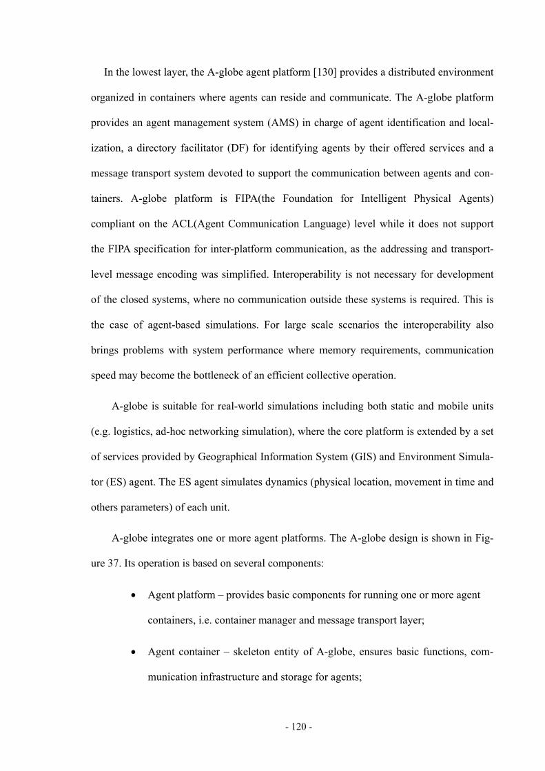
- 120 -

In the lowest layer, the A-globe agent platform [130] provides a distributed environment

organized in containers where agents can reside and communicate. The A-globe platform

provides an agent management system (AMS) in charge of agent identification and local-

ization, a directory facilitator (DF) for identifying agents by their offered services and a

message transport system devoted to support the communication between agents and con-

tainers. A-globe platform is FIPA(the Foundation for Intelligent Physical Agents)

compliant on the ACL(Agent Communication Language) level while it does not support

the FIPA specification for inter-platform communication, as the addressing and transport-

level message encoding was simplified. Interoperability is not necessary for development

of the closed systems, where no communication outside these systems is required. This is

the case of agent-based simulations. For large scale scenarios the interoperability also

brings problems with system performance where memory requirements, communication

speed may become the bottleneck of an efficient collective operation.

A-globe is suitable for real-world simulations including both static and mobile units

(e.g. logistics, ad-hoc networking simulation), where the core platform is extended by a set

of services provided by Geographical Information System (GIS) and Environment Simula-

tor (ES) agent. The ES agent simulates dynamics (physical location, movement in time and

others parameters) of each unit.

A-globe integrates one or more agent platforms. The A-globe design is shown in Fig-

ure 37. Its operation is based on several components:

• Agent platform – provides basic components for running one or more agent

containers, i.e. container manager and message transport layer;

• Agent container – skeleton entity of A-globe, ensures basic functions, com-

munication infrastructure and storage for agents;

- 121 -

• Services – provide some common functions for all agents in one container;

• Environment simulator (ES) agents – simulates the real-world environment

and controls visibility among other agent containers;

• Agents – represent basic functional entities in a specific simulation scenario.

Figure 37. A-globe System Architecture Structure

Simulation scenario is defined by a set of actors represented by agents residing in the

agent containers. All agent containers are connected together to one system by the GIS ser-

vices. Beside the simulation of dynamics the ES agent can also control communication

accessibility among all agent containers. The GIS service applies accessibility restrictions

in the message transport layer of the agent container.

On top of the A-globe agent platform resides the multi-agent architecture, providing

the base agents, structures and semantics for implementing urban demand responsive

transportation information intelligent control system [131]. The agents are of four kinds:

- 122 -

the user agent, which is in-charge of the communication with the different parties involved

(vehicles, clients, other systems) by means of different devices; the node-station agents,

which are in-charge of processing, assigning and scheduling the received trip requests en-

capsulate the assignment and scheduling of the transportation requests processed by the

system; the taxi agent, which is in-charge of modeling each real vehicle for the system; and

the transport-admin agent, which is in-charge of all agents (taxis, node-stations).

Finally, over the multi-agent architecture layers an urban demand responsive transpor-

tation system layer is implemented. By extending and implementing the agent-based

system provided by the architecture, a dynamic trips planning and traffic control system

can be developed.

5.2.2 The Definition of Agents

This section describes the main agents in the multi-agent architecture used for urban

demand responsive transportation intelligent control system.

User Agent

This kind of agent represents a human user and their (allowed) interactions with system.

It is responsible for capturing all the client’s requirements. It provides communication and

interoperability between the end user and the urban demand responsive transportation in-

telligent system.

Node-station Agent

This kind of agent is to model each real geographical node-station for the system. This

agent is in-charge of processing, assigning and scheduling the received trip requests. It is

responsible for coordination with the other agents and the administration of the transporta-

- 123 -

tion service. It helps in the collaboration among agents that provide support to related func-

tions, such as the matching of request to vehicles, the geographical data access, the

accountability of the transactions and the service payment among others.

Taxi Agent

This kind of agent is in-charge of modeling each real vehicle in the system. It processes

the trip plan of the vehicle and provides interoperability between the vehicle and the DRT

system. Taxi agents make proposals for the actual plan, process change information with

the node-station agent, update the plan and reschedule the remaining trip requests.

Transport-admin Agent

This kind of agent is in-charge of all agents (taxis, node-stations, users). It can set: how

many taxi agents will start, how route planning and intercommunication they will use

matching transport requests with available vehicles. It manages service descriptions com-

ing from vehicles side and client’s side.

5.2.3 Agent Planning Sequence Model Design

The taxi agent planning sequence model design could be carried out by either a cen-

tralized model or a decentralized model. The differences among these two options are

briefly described and then we present our multi-layer distributed hybrid planning model.

The centralized model (See Figure 38) considers the optimization of the entire system

as the most important thing. For this reason, it pursues the minimization of all disutility

function that considers the agent operator (number of vehicles required, occupancy and

slack times) [132] and the served users (effective waiting time, effective excess ride time).

- 124 -

The decentralized model (See Figure 39) is based on self-interested actors. This

means that each agent seeks the maximization of its own utility.

The hybrid model uses a third actor, the planner for applying filtering policies [133].

The taxi agent behaves in a self-interested way as in the decentralized model approach

[134]. The difference from the decentralized model is the hybrid planning algorithm for

transport tasks allocation.

Centralized Model

Figure 38. Centralized Model

In the centralized model, it focus is on optimization of the global utility for the system.

Transport-admin agent can control other three kind agents, and choose the trip plan for cli-

ents.

- 125 -

Since the urban demand responsive transportation information system is not always lin-

ear, when something is amiss in the communication between the agents, the centralized

system will be unstable. (See Figure 38)

Decentralized Model

Figure 39. Decentralized Model

In the decentralized model, each agent is interested in maximizing its utility (See Figure

39). Every agent can propose his trip plan to clients. In the decentralized model is based on

self-interested actors. This means that each agent seeks the maximization of its own utility.

In our situation, node-station agent to model each real geographical node-station for the

system, they do not move. The taxi agents are in-charge of modeling each real vehicle in

the system, they are moving in real-time. It is a distributed real-time situation. So decen-

- 126 -

tralized model and centralized model is difficult to find good solution. Then we will intro-

duce our multi-layer distributed hybrid planning model.

Multi-Layer Distributed Hybrid Planning Model

Figure 40. Agent Planning Domain Framework

- 127 -

In Figure 40 we can see: each taxi agent has graph with its particular edges (costs of

edges) and a planning domain. According to it, taxi agent makes its plan of path. Because

of traffic unpredictability (traffic jams, etc.), taxi agents need to communicate with other

agents exchange information. Therefore each taxi agent makes own statistic of pass times.

It updates it by means of own experience and experience of the others, that are transmitted

among them by sending messages.

In our approach, every taxi agent is moving and the trip requests are random. So it is a

dynamic distributed situation. If all the agents communicate together online, it will be

slowly and unstable. Hence each taxi has a limited range of planning domain it need not

communicate with all taxi agents. The taxi agent can communicate only with taxis agents

or node-station agents in its planning domain, the information interchange is performed

when other agents entry to the planning domain. It also ensures change while each meet-

ing. So they can change their plan and use another path.

Taxi planning system ensures route planning and communication with the view of im-

proving planning. It consists of two main parts. First part is taxi agents planning and re-

planning paths within its planning domain. Second part is node-station communicating in

real time. It ensures right interchange and using information about traffic situation and pas-

sengers’ trip requests. (See Figure 41)

As mentioned above, in the multi-layer distributed hybrid planning model we have:

1) A multi-layer distributed hybrid structure is used.

2) The node-station agent applies filtering policies.

3) The taxi agent makes proposals for the actual plan, process change information with

the node-station agent in its planning domain, updates the plan and reschedules the remain-

ing requests, transport passengers.

- 128 -

Figure 41. Agent Multi-Layer Planning Framework

- 129 -

In the transport-admin agent layer, user agent’s job is to represent the client and his de-

cisions of the transportation request. So it is responsible for the result. Since the real client

does not directly communicate with the taxi agent, the user agent also constitutes a kind of

client towards the transportation system, which is represented by the node-station agent.

So when the clients change their requests in a dynamic scenario to deal with unexpected

situations, the user agent also has responsibility for communicating the client about any

subsequent changes to the original deal. These unexpected situations must also be commu-

nicated with the other agents though transport-admin agent. The user agent must

communicate to the transport-admin agent about changes on the clients’ desires (e.g.

change the lieu, delays, and trip cancellations). The transport-admin will implement a ne-

gotiation with the node-station agent about the changed request.

In the node-station agent layer, the node-station agent gives the client (through taxi

agent) the most suitable trip solution offered by the planning together after filtering a list of

proposals. The node-station agents do not move, like the station in the geography map. At

the same time, the node-station agent holds a request profile containing the client’s prefer-

ences concerning the trip. It also holds some negotiation capabilities with the other node-

station agent in real time. The node-station agent processes all the client’s requests coming

through the User agent. It is the agent who in charge of executing a negotiation role in the

layer. In addition, the node-station is in charge of implementing the assignment through

filtering policies and the negotiation process. It holds a list containing the trip requests be-

ing processed and a list of filtering policies to apply to the trip solutions. Before the taxi

agent gives the proposals to the node-station agent, it will communicate with the other

agents that manage the trip plan of the vehicle and other traffic information in its planning

domain.

- 130 -

In the taxi agent layer, when a taxi agent communicates with other agents in its plan-

ning domain, if there is not any node-station agent in it, the planning model will be

“decentralized”, and in the plan logic we will chose a trusted third party acting as auction-

eer. The details we will describe in section 5.2.4. (See Figure 42)

Figure 42. Taxi Agent “Decentralized” Planning Model

If there is a higher lever node-station agent in it, the planning model will be centralized

(See Figure 43). When we set the taxi agent planning domain, we should make sure that

there is not two node-station agents in its planning domain. In this situation, we will

choose node-station agent acting as auctioneer in planning logic.

- 131 -

Figure 43. Taxi Agent Centralized Planning Model

When the node-station agent receives the trip-proposals from the taxi agent, it can

implement different filtering policies that include: the minimum number of used vehicles,

the waiting time, the travel time, and the total traveled distance. This point is very impor-

tant for the client that the system just like a “Black Box” [135]. The clients propose the

request to the User agent and get the best solution for his request.

To sum up, the multi-layer distributed hybrid planning model is able to provide reso-

lution for the gaps in performance for our distributed real-time situation. In next chapter,

we examine the effectiveness of the proposed method by computational experiments.

- 132 -

5.2.4 Planning Domain Based Multi-agent Plan Logic

In the demand responsive transportation system, a general formulation of a client’s de-

mand function is:

).....( 321 ixxxxFY ••••=

Where Y is the dependent variable (level of demand) and xi (i = 1, 2..., n) are the ex-

planatory variables. The demand function reflects the behavior of an individual client,

whose preferences dictate the particular functional form of the relationship, or it may be

formulated to explain the behavior of an aggregate group of individual client.

A particular specification of the demand function which is often used to analyze client’s

travel demand is expressed in terms of ‘generalized costs’ (time, money…). This concept is

an attempt to summarize the ‘cost’ of a journey by adding together the various components

of time or money spent. The operation system can be formulated as the following optimi-

zation problem:

Minimize 01cmqaAC M

i iiT ∑=++•= β

Where:

ACT is the all generalized cost of the journey at time T.

β is the value of coefficients.

M is a set of all passengers.

m is the monetary cost of the journey.

ai is the value of time associated with time component i.

- 133 -

qi is the time required to complete the journey divided into the various components i of

traveling time: like a get-on delay time of passenger i, a get-off delay time of passenger i,

the travel time.

c0 is the residual component of the ‘cost’ of making a journey which is not a function of

the monetary cost or the time involved but is a ‘cost’ associated with user’s special re-

quirement component. This cost may represent many different aspects of travel, e.g. the

effort involved in taking heavy or bulky baggage on a trip or that part of the discomfort or

general inconvenience which is not a function of the time duration of the journey. In some

models this component also represents the different propensities to travel of different seg-

ments of the population, grouped by income, sex, age etc and will take different average

values in all these categories. The generalized cost function represents the traveler’s will-

ingness to pay to reduce the waiting, walking or trip time. The residual effort component is

also measured in monetary units.

In our multi-layer distributed hybrid planning model, we propose a special approach to

multi-agent planning logic for taxi agents and node-station agents, extending an existing

resource-based planning approach. As the earlier section described situation of our model,

we assume that each of the agents has a plan available to satisfy their goals. In order to

lower their costs, two or more agents investigate whether they can cooperate together in

their planning domain.

In [136], Mathijs de Weerdt (2003) introduced a resource oriented representation of ac-

tions and state called the Action Resource Formalism (ARF). His main idea is that in

carrying out a plan an agent possibly produces side products that can be used as resources

by other agents. As a result, other agents can discard some of its planned actions. This

process of exchanging products, called plan merging, results in distributed plans in which

- 134 -

agents become dependent on each other, but are able to reach their goals more efficiently.

The formalism is a resource logic based on the notions of resource, skill, goal, and service.

In the Action Resource Formalism (ARF) planning merging logic, two agents can co-

operate if one agent produces a resource – one that is not directly needed for goal

satisfaction, but as a byproduct – that is needed by the other agent. Both agents may agree

to cooperate by exchanging resources. That is to say, the agent producing the resource al-

lows the other agent to use it. As a result, the resource that was originally produced as a

byproduct becomes a sub-goal for the agent.

Several potential problems may arise during merging of two plans. Plans may conflict

and get into deadlock situation. Normally it happens when agents require the same re-

source for correct execution, or the prescribed order of actions may lead to dead-lock, e.g.,

both have to wait for the other to finish the certain action. For example, consider the fol-

lowing two goals:

Agent1: G1.underCondition(A), B is one of the subgoal of G1

Agent2: G2.underCondition(B), A is one of the subgoal of G2.

Assume that agent1 is pursuing G1 under condition A, but has not yet reached subgoal

B. The agent2 is pursuing G2 under condition B, but has not yet reached subgoal A. In this

situation, the system will be into deadlock. So in Mathijs de Weerdt’s model, he used auc-

tion mechanism exchanging resources. He assumed one of the agents acts as an auctioneer

and collects all requests of all agents. For each request an auction is held, in which all

agents, other than the requesting agent, may offer to deliver the requested resource. The

auctioneer ensures that all constraints are satisfied and that the exchange actually takes

place, resulting in a cost reduction. We assume that agents are always willing to cooperate.

- 135 -

The problem is that for every plan merging, we need to do “auction” collecting all re-

quests of all agents, so how many agents in the system? If there are many mobile agents in

the system, it will be slow and difficult to avoid deadlock. For example, in our real-time

distributed situation, there are many taxi-agents moving in real-time. If we use auction

mechanism merging all the agents’ plan together in real-time, the system will be slow and

not stable. So as we introduced before, in our proposed model there are three layers, taxi-

agents and node-station agents plan together in their planning domain.

We propose a special planning domain based multi-agent planning logic, extending an

existing resource-based ARF (Action Resource Formalism) planning approach. We also

use many-sorted first-order language to describe our framework [137]. At first we intro-

duce many-sorted language described primitive ARF (Action Resource Formalism) main

elements notions like goals, resources, action, plans, and our special element planning

domain. Then we describe the planning domain based multi-agent plan merging logic and

its algorithm.

Definition 1. The alphabet of a many-sorted first-order language consists of the follow-

ing sets of symbols:

A countable set S∪{bool} of sorts (or types) containing the special sort bool, and such

that S is nonempty and does not contain bool.

• Logical connectives: ∧ (and), ∨ (or), ⊃ (implication), ≡ (equivalence), all of

rank (bool.bool, bool), ￢ (not) of rank (bool, bool), ⊥(of rank (e, bool));

• Quantifiers: For every sort s ∈S, ∀s (for all), ∃s (there exists), each of rank

(bool, bool); For every sort s in S, the equality symbol =． s, of rank (ss, bool).

- 136 -

The symbols consisting of:

• Sorts: Sorts = {s1, s2, . . . , sn, . . .}.

• Variables: Vars = { 1sx , . . . , 1

nx ,…. . . .} for each s ∈ Sorts; we use Var =∪s�Sorts

Vars to denote the set of all variables.

• Predicate symbols: Pred = {p,q, . . .} with rank r : Pred → Sorts∗ .

• Function symbols: Funs = {f,g, . . .} and rank r : Funs → Sorts+ × {s} for each s

∈ Sorts.

• Constants: Cons = { 1sc , . . . , n

sc , . . .} for each s∈Sorts.

Resource

For the plans, the resources are required to achieve a goal. This attribute captures the re-

source requirements of all actions within the plan and does not include the resource

requirements of any sub-goals of the plan. We model a real process, like transportation in

our DRT systems, by an action. Each resource fact represents a particular atomic product

or object with all its properties at a specific time and place. This implies that for each ob-

ject many possible resource facts exist, but only one at a time. Resource facts may also be

used to denote more abstract ‘products’, such as possibilities and availabilities. The proper-

ties of a resource are described by the terms in our language, and are defined for all

planning agents in a specific domain. A fundamental property of resources is that they can

be consumed and produced by actions. We use these actions combining together to achieve

certain goals in agent’s planning domain. This kind of actions combing together is called as

plan.

- 137 -

A resource fact, or simply resource, in many-sorts first order language formula p(t1 : s1,

t2 : s2, . . . , tn : sn). The terms sj are also called the attributes of resource p with attribute

values tj .

As an example, take a resource fact:

Taxiagent(1234 : id, Rouen1 : loc, [90, 100]: time, [123,124]: planningdomain)

It is referring to the taxi with identification 1234 at location Rouen1 at time interval [90,

100], taxi123 and taxi124 in his planning domain. This point is different from resource

based planning logic before, in our model taxi agents change information and planning to-

gether in his planning domain.

Resource scheme is used to indicate a set of sources sharing some attributed. It is useful

to denote arbitrary resources that are ground instances of a resource scheme. For example,

Taxiagent (x : id, rouen : loc, I : time)

It is a resource scheme denoting some taxi at Rouen, where we do not care about the

time interval I it is available.

Definition 2. A set of resources R satisfies an extended resource scheme (RS, C), RS is a

set of resource schemes, and C is a set of constraints for terms with variables occurring in

resources in RS,, abbreviated as R |= (RS, C), if there exists some resource-identity preserv-

ing ground substitution θ with respect to RS such that

1. RSθ ⊆ R,

2. |= Cθ, i.e., every constraint reduces to true under θ.

If we want to specify the substitution θ used to satisfy the extended resource scheme,

we write R |=θ (RS, C).

- 138 -

Example: Consider a passenger p(x: loc, I1 : time) at location x at time interval I1, wait-

ing for a (taxi)-ride ride(x : loc, y : loc, c : cap, I2 : time) from location x to y, having c free

seats and occurring in time interval I2. To help the passenger it is required that c > 0, and I1

∩ I2 = Ø. This is expressed by the following extended resource scheme:

({p(x : loc, I1 : time), ride(x : loc, y : loc, c : cap, I2 : time)}, { I1 ∩ I2 = Ø, c > 0}).

Every set R of resources containing at least one ride and one passenger resource meet-

ing these constraints will satisfy this extended resource scheme.

A resource fact is the concise description of an object (resource) that is relevant to an

agent with respect to the planning problem at hand. Such a resource is either a physical ob-

ject such as a taxi or a passenger, or an abstract conceptual notion such as an opportunity to

travel. Syntactically, an atomic resource fact is denoted by a predicate name together with a

complete specification of its attributes, together with their values. The predicate name

serves to indicate the type of resource mentioned in the fact (e.g., a taxi or a passenger). If

taxi is a resource type, having an attribute location loc and an attribute num, then taxi (8:

num, A: loc) is an atomic resource fact describing taxi number 8 in A. Since similar re-

sources (i.e., resources with the same type and the same values for the attributes) may

occur multiple times in the same plan, we add to each resource a unique occurrence identi-

fier of sort identity, i.e., a special index that is used exclusively to distinguish between

different occurrences of a resource in a plan. A resource of type t with i as (the value of its)

occurrence identifier is denoted as ti(. . .).

Values of attributes may be ground (i.e., constant), but may also be variables or func-

tions. In the latter case, a resource fact describes a set of ground resource facts (instances)

of the same resource type. For example, the following resource refers to all taxis in loca-

tion A: taxi (n: num, A: loc). To specify one specific ground resource fact denoted by such

- 139 -

a general resource fact, we introduce the notion of a substitution. A substitution θ replaces

variables occurring in a resource r by terms of the appropriate sort like. We also use rθ to

denote the resource r’ that results from replacing the variables occurring in r according to θ

like in ARF. If R is a set of general resources, Rθ is a shorthand for {rθ | r∈R}.

Goals

Some resources an agent already has, others he needs to obtain. In general, such an

agent does not care about obtaining a specific (unique) resource as a goal g, but only a re-

source having some specific properties. So we will conceive an individual goal g as a

resource scheme. Even more generally, we may want to obtain a set of goals meeting some

constraints. Therefore, we define goals and goal schemes analogously to resources and ex-

tended resource schemes as follows:

Definition 3. A goal g is a resource scheme. A goal scheme Gs is an extended resource

scheme Gs = (G, C), where G is a set of goals. G = {g1, . . . , gn}.

As goal schemes are extended resource schemes, we also use R |= G to express that the

resource set R satisfies the goal G. if there exists a ground substitution θ such that Gθ⊆R,

i.e., there is a set of ground instances of the goals that is provided by the resources in R.

Two resources r1 and r2 are called equivalent, denoted by r1 ≡ r2, when they are equal ex-

cept for the value of their occurrence attribute. Resource facts are used to model the state

of the world (as far as it is relevant) by enumerating the set of resource facts that are true at

a certain time point. Possible transitions from one state to another are described by actions.

An action is a basic process that consumes and produces resources. An action o has a set of

input resources in(o) that it consumes, and a set of output resources out(o) it produces. Fur-

thermore, an action may contain a specification param(o) of some variables that occur in

- 140 -

the set of output resources as parameters of the action. To ensure that each output resource

out is uniquely defined, it may only contain variables var(out) that already occur in the in-

put resources or in the set of the parameters. This is formally defined as follows.

Action

Action is a rule of the form a: Rs2 ← < Rs1,C>, a is the name of the action, Rs2 is set

of resources produced by a, Rs1 is the set of resources consumed by a and C the set of con-

straints on Rs1.

Definition 4. An action specification is a formula:

oid(x1, . . . , xn) :Ф{inid,−i|1≦ i ≦m} ⇒ Ф{outid,i|1≦i≦k} where

1. id is a variable of sort identity,

2. x1, . . . , xn are the parameters of the action,

3. Ф {inid,−i|1≤i≤m} is a conjunction of general (input) resources inid,−i(. . .),

4. Ф {outid,i|1≤i≤k} is a conjunction of general (output) resources outid,i(. . .), such that

for all 1≤i≤k, var(outid,i)⊆Uj var(inid,j)U {xl | 1≤l≤n}.

Remark: The value (id,−i) of the occurrence id for the i-th input resource is inherited

from the value of the occurrence identifier of the action o in which its is used. Analogously

the value (id, i) of output resources is constructed. As can be seen later on, this mechanism

provides us with unique occurrence labels of resources in plans.

Example : Consider the following action

moveid(y : loc) : taxi(id,−1)(n : num, x : loc) ⇒ ride(id,1)(x : loc, y : loc) ∧ taxi(id,2)(n :

num, y : loc)

- 141 -

This action specifies how a taxi may move from a source location x to a destination y

and requires the taxi to be present at the source x. It “produces” a taxi at the destination

and the ride opportunity (for passengers) to travel with this taxi from x to y. Let O be a fi-

nite set of action specifications. The set O is said to be a set of (concrete) actions over O if

(i) every action occurring in O is obtained from an action oid() in O by substituting a

unique ground value v for its occurrence identifier id and (ii) variables in actions are stan-

dardized apart, i.e., for each o≠ o’∈O we have var(o) ≠ var(o’). A concrete action o ∈ O

can be applied to a set of (ground) resources R if there exists a ground substitution θ such

that in(o) θ⊆R. Application of this action to R results in consuming the set in(o)θ of input

resources while producing the set out(o) θ. The result of o applied to R (under θ) therefore

is a resource transformation: starting with R, the set R \ in(o)∪out(o)θ is produced. The set

res(O) is the set of all resources mentioned in the input in(o) or output out(o) of actions o

∈ O. The set cons(O) specifies the set of all resources consumed using actions in O:

cons(O) = ∪o∈ O in(o), while the set of resources produced equals prod(O) = ∪o∈ O

out(o).

Plan

In general, a single action applied to an initial set of resources is not sufficient to

achieve a desired state. Often, a set of actions have to be applied in some partial order to

produce the desired effect. A specification of only the ordering of actions, however, in gen-

eral is not sufficient to describe a plan in sufficient detail. ARF also need to specify for

each consumed resource, which produced resource it is dependent upon. Such a partially

ordered set of actions with a specification of the dependency relation between resources is

- 142 -

called a plan. To specify how actions are interrelated, we also use the notion of a depend-

ency function.

Definition 5. Let O be a set of (concrete) actions. A dependency function is an injective

function d : cons(O) → prod(O) ∪ {⊥} specifying (in a unique way) for each resource r

to be consumed which resource r’ produced by another action is used to provide r (or ⊥ if

r is not produced by an action in O, i.e., r is an input resource).

Sometimes we need the inverse d−1 of d, which is defined as follows: for every r’

∈ prod(O) such that d(r) = r’, d−1(r’) = r, and for every r’ ∈ prod(O) not occurring in

ran(d), d−1(r’) = ⊥. As mentioned before, plans are composed of partially ordered actions.

Since a dependency function d specifies an immediate dependency of input resources of an

action on output resources of another action, d can only specify a valid dependency if (i)

the resources involved are equivalent and (ii) d generates a partial ordering of the actions

in O.

The first requirement is met if there exists a substitution θ such that for two resources r

and r’, d(r) = r’ implies rθ ≡ r’ θ , that is θ is a unifier for every pair of resources (r, d(r)).

In particular, we are looking at a most general unifier (mgu) θ with this property.

The second condition requires that there are no loops in the dependency relation be-

tween actions generated by d: we say that o directly depends on o’, abbreviated as o’ <<d o,

if resources r ∈ in(o) and r’ ∈ out(o’) exist such that d(r) = r’. Let <d = << +d be the transi-

tive closure of <<d. Then the second condition simply requires <d to be a (strict) partial

order on O.

Now a plan can be defined as follows.

- 143 -

Definition 6. A plan P over a set of actions O is a triple P = (O, d, θ) where d is a de-

pendency function specifying dependencies between equivalent resources and generating a

partial order <d on O, while θ is the mgu of all dependency pairs (r, d(r)) with r, d(r) ∈

res(O). The empty plan (Ø,Ø,Ø) is denoted by ◇.

Given a plan P = (O, d, θ), the set In(P) = {rθ | r ∈ cons(O), d(r) = ⊥} is the set of in-

put resources of P, i.e., the set of resources not depending on other resources in the plan.

Analogously, the set Out(P) = {rθ | r ∈ prod(O), d(r) = ⊥} of output resources of P is the

set of resources that are not consumed by actions in the plan. Furthermore, we define

prod(P) = prod(O) θ and cons(P) =cons(O) θ. Note that resources from prod(P) may be

consumed by other plans to produce resources.

A planning problem Π= (O, I,G) is given by a set of ground initially available resources

I, a set of goal resources G, and a set of action specifications O that can be used for this

problem domain to transform resources. A solution to such a planning problem п is a plan

P = (O, d, θ) where O is a set of concrete actions over O and there exists a substitution Υ

such that In(P)⊆ I and Out(P)Υ |= G.

Planning domain

Definition 7. Planning domain is the domain range for agent’s communication. The

agent only can communicate and exchange information with other agents in his domain

range. A planning domain of the agent ai∈A is a tuple PDi= (Pj, aj) where Pj is plan of

agent aj in the agent ai planning domain, A = {a1, a2, . . . ,an} is a set of agents.

For a set of agents A = {a1, a2, . . . , an} that each has one plan P1, P2, . . . , Pn for its

problem Π1, Π2, . . . , Πn . Ppdi is plan after agent ai planning together with other agents

- 144 -

in his planning domain. We can now combine these plans into one composed plan

(Ppd1║Ppd2║ ··· ║ Ppdn) for the combined problem Π. An independent combination of

their plans can be considered as a model of their joint plans:

Pi= pdjPDj

Pi

U∈

)( aAa

POut∈U |= a

AaG

∈U and a

AaI

∈U |= )( a

AaPIn

∈U

That is mean: the agents jointly are able to satisfy the joint goals G using their joint re-

sources I. So we can use the plan reduction techniques in the every agent’s planning

domain to deal with the multi-agent cooperation planning problem.

Planning domain based multi-agent plan merging logic

The main idea of planning domain based multi-agent plan merging is that agents can re-

duce the cost (action) of their own plan by communication and cooperation with other

agents in his planning domain. Agent can remove actions for which the results (the re-

sources produced by these actions) are readily available at other agents in his planning

domain.

Plan reduction:

In the planning domain, we also use plan reduction like in AFR. The different is: the

plans reduce and merging in the agent’s planning domain. For each concrete action o ∈ O

there is a positive integer value cost (o), representing the cost of executing o. Agents, once

having conceived a plan P = (O, d, θ) will aim at reducing the cost cost(P) = ∑ ∈Ooot )(cos

of their plan, while maintaining goal-reliability. To reduce the costs of a plan an agent

- 145 -

therefore might try to remove some action o from its plan, by replacing every output re-

source r of o that is used in the plan, i.e. d−1(r) ≠ ⊥, by another other, freely available

resource r’ occurring in the current plan or by an input resource of o. The resources r’ that

is not used in a plan to attain the goals is called free resources and are defined as follows:

Definition 8. Given a plan P = (O, d, θ) that is a solution to a problem Π= (O, I,G), and

a substitution θ G such that G θ G ⊆ Out(P), the set of free resources is defined as Free(P,

Π) = (I \ In(P)) U (Out(P) \ G θ G).

If using Free (P, Π) U in(o) θ, every output resource can be replaced such that a

cheaper valid plan P’ can be obtained, we say that P is reduced by removing o.

Note that if o cannot be removed, a nonempty subset of its (used) output resources can-

not be replaced. We call this set the request set RequestSet(P, Π, o) belonging to o and

note that it contains the set {r | r ∈ out(o), d−1(r) ≠ ⊥ }\ (Free (P, Π) U in(o)). Viewed

from a multi-agent perspective, these request sets can be used for resource transactions be-

tween agents: if free resources are available from other agents in his planning domain, we

can reduce the plan P exists if these free resources are sufficient to attain RequestSet.

Definition 8. Free resources of a multi-agent plan: Given a multi-agent planning prob-

lem {(Oa, Ia, Ga) | a ∈ A}, and an action o ∈ O for an agent i ∈ A, in agent i planning

domain a set of independent embedded agent plans {Pa | a ∈ PDi}. Then the set of free

resources with respect to the action o is given by Free ( −oiP, )∪ { }U j\Aj∈

Free(Pj).

Multi-agent plan reduction: Given a multi-agent planning problem { Πa | a ∈ A},

where Πa = (Oa, Ia,Ga), an action o ∈ O for an agent i ∈ A, in agent i planning domain a

set of independent embedded agent j plans {Pj | j ∈ PDi}, where Pa = (((Oa, da, θa) , Ia, dIa,

θIa) ,Ga, dGa, θGa). If

- 146 -

Free ( −oiP, )∪

{ })(

iPDj\j

AjPFree

∈∈U |= In( +

oiP, )∪(Gi \ 1−Gid (Out ( +

oiP , )) ,

then a partial injective function

f : In( +oiP , )∪(Gi \ 1−

Gid (Out( +oiP , ))→Free( −

oiP, ) ∪{ }

)(iPDj\

iAi

PFree∈∈U

can be found such that the tuple ({(Oa, da, θa) | a ∈ A}, d*, θ*) is a multi-agent solution

where d* ⊆ f is a partial dependency function U Aa∈ In(Pa) → U Aa∈

Out(Pa) and θ* is a

substitution.

Theorem 1. Given a set of agents A, for each agent i ∈ A a problem Π i and a plan Pi

that solves this problem, the action o in the plan Pj of agent j (agent j in agent i planning

domain) can be removed if

{ }),(

iPDj\ii

AiPFree Π

∈∈U |= RequestSet (Pj , Π i , o).

About proof of resource based multi-agent plan reduction theorem can be found in [5].

This reduction property is used in the plan merging algorithm to be discussed next.

Plan merging:

In Action Resource Formalism (ARF), it uses auctioneer mechanism algorithm to ex-

change of resource facts. It assumes that one of the agent or a trusted third party acts as the

virtual auctioneer. The problem is that it chose one auctioneer for the entire agents plan

merging make system slow and difficult to avoid deadlock especially for real-time system.

In our model, we also use auctioneer mechanism in agent planning domain plan merg-

ing. When in one taxi-agent planning domain, there is one high lever station-agent, we will

choose the station-agent acting as auctioneer. If there is only the same lever taxi-agents in

- 147 -

his planning domain, we will assume that a trusted third party acting as virtual auctioneer.

And for avoiding deadlock if one taxi-agent in one station-agent planning domain, it will

be not acting as auctioneer in other agents’ planning domain at the same time.

The planning domain based plan merging algorithm (Algorithm 1.) works as follows:

Agents communicate with other agents in his planning domain to choose the auctioneer in

the agent planning domain. The auctioneer announces when the agents in the planning do-

main can start the plan merging, thereby announcing some minimum allowed cost

reduction value. All agents in his planning domain deposit their request sets with this auc-

tioneer. Each request set corresponds with the removal of an action from an agent’s plan

and contains a set of resource facts the agent needs to remove the particular action. Fur-

thermore, the request contains a cost reduction value defined by the difference in costs

between the old plan and the resulting plan if the exchange would succeed.

The auctioneer deals with the request with the highest potential cost reduction first. All

the agents openly announce their cost reduction values. Right before each auction round

starts, the requesting agent (ai) is asked for the specific set of resource facts that has to be

replaced by resource facts of other agents – this set is called the RequestSet. This set is not

necessarily equal to the set in the initial request, since other exchanges influence the avail-

ability of resource facts for the agents. Next, the set of requested resource facts is sent to

each agent, except to ai. The agents in the planning domain return all their free resource

facts for which there is an equivalent one in the request set RequestSet, and include the

price of each of their offered resource facts. When all bids (collected in R’) are collected by

the auctioneer, it selects for each requested resource fact the cheapest bid (Vickrey (1961)

auction).

If for each resource fact in RequestSet a replacement can be found, the requesting agent

ai may remove the corresponding action(s). Furthermore, we have to add dependencies be-

- 148 -

tween the providing agents and the initial resource facts for the requesting agent. At the

end of each successful exchange each involved agent has to update the cost reduction val-

ues of all of their requests, because this value can change as the agent can now have more

or less resource facts available. One could repeat this process until none of the auctions has

been successful done.

We can see that the planning domain based agent plan merging algorithm is a distrib-

uted any-time algorithm, because it can be stopped at any moment. And the system will not

be dead that even in some agent’s planning domain have dead-lock problem. If the algo-

rithm is stopped, it still returns an improved set of agent plans, because it uses a greedy

policy to dealing with the requests with the largest potential cost reduction first.

Algorithm 1. planning domain based plan merging

1. choose the auctioneer in each agent’s (ai∈A) planning domain PDi.

2. auctioneer broadcasts minimum allowed cost reduction.

3. auctioneer retrieves requests with their cost reduction from all agents in planning

domain.

4. while some requests left do

4.1. get the request with the largest cost reduction.

4.2. ask the requesting agent ai for the required resource facts RequestSet.

4.3. for each agent aj ∈ PDi, aj ≠ ai do

4.3.1. ask aj for free resource facts equivalent to RequestSet.

4.3.2. add these resource facts to R’.

4.4. if R’ ⊇ RequestSet then

4.4.1. let R” ⊆ R’ be the cheapest set that satisfies RequestSet.

4.4.2. add for each r ∈ RequestSet the corresponding dependency to R”.

4.4.3. remove as much actions as possible from the plan Pi of ai.

4.4.4. for each involved agent in the planning domain, update the cost reduction

of all requests.

- 149 -

Example: In taxi agent T1planning domain, there is taxi agent T2 and node-station

agent N1. Suppose that a taxi agent T1, starting in A, has the plan to put down a passage1

at station1 and put down passage2 at station2 , and get a passenger3 from station1 to sta-

tion2. Taxi agent T2 starts in B, has the plan to put down a passage4 at station1, and get a

passenger5 from station1 to station2. Their initial routes are shown in Figure 44. Each taxi

has at least 4 passenger seats.

Figure 44. Taxi Agent T1 ad T2 Initial Routes

- 150 -

When these agents are cooperating and plan merging together, they can significantly re-

duce the distance traveled and costs by sharing their capacities and travel. In taxi agent T1

planning domain, there are taxi agent T2 and high lever station-agent N1, so N1 will be

acting as auctioneer. (See Figure 45) If there is no node-station agent, we will choose a

trusted third party acting as virtual auctioneer.

N1

T1T2

Ni : Node-station agent iTi : Taxi agent i

Taxi agent1 planning domain

AB

Auctioneer

Figure 45. Plan Structure in Taxi Agent T1 Planning Domain

The initial plans of taxi agent T1 and taxi agent T2 are represented in the action re-

source formalism by the dependency graph shown in Figure 46 and Figure 47.

- 151 -

Figure 46. Action Resource Graph of Taxi Agent T1

- 152 -

Figure 47. Action Resource Graph of Taxi Agent T2

- 153 -

Running planning domain based plan merging algorithm in taxi agent T1 planning do-

main, taxi agent T1 and T2 return a set of requests to the auctioneer node-station agent N1.

For taxi agent T1, it finds that it can reduce its plan with two actions if it is able to obtain a

resource ride (A, N1) and ride (N1, N2) from one of the other agents. For taxi agent T2, it

finds that it can reduce its plan with two actions if it is able to obtain a resource ride (B,

N1) and ride (N1, N2) from one of the other agents. Each request consists of a resource

and a number of the potential cost reduction. The requests are put in a priority queue based

on this cost reduction. Unfortunately, there is not resource for taxi agent T1 request ride

(A, N1), and for taxi agent T2 request ride (B, N1) either. So these requests do not lead to a

success. But for request ride (N1, N2) both taxi agent T1 and taxi agent T2 can obtain

from each other. To satisfy taxi agent T1 request, we can not remove any action because

there is passage2 on taxi1 who want go to station N2. We can see that to satisfy taxi agent

T2 request can remove one action. So this request has the highest priority and is treated by

auctioneer first. Then the actions move (N1, N2) can be removed from the plan of taxi

agent T2. When this has all been done, the auctioneer continues with the next request if

there are any other requests. The result of the merging plan is depicted in Figure 48.

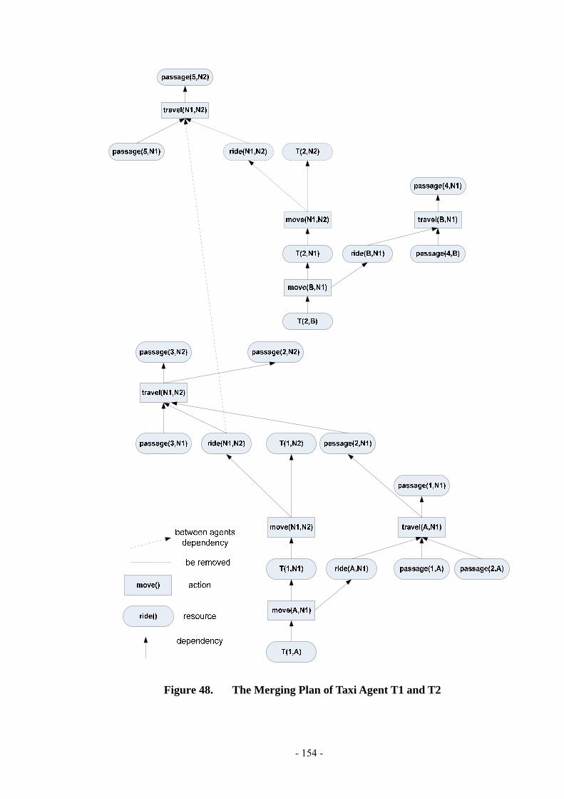
- 154 -

Figure 48. The Merging Plan of Taxi Agent T1 and T2

- 155 -

Chapter 6. Multi-agent Based Multi-Layer Distributed Hy-

brid Planning DRT System Prototype and Experiments

Analysis

In multi-agent simulation, Simulation platform is very important for system design. So

in next section, we will first introduce simulation platform. Then we will introduce proto-

type implantation and experiments analyze.

6.1 Simulation Platform

6.1.1 Programming Language

There are many different multi-agent construction platforms or frameworks available,

some of which are for academic and educational research, while others are built for com-

mercial applications. Agent construction tools use the principle of object-oriented design

and programming to encapsulate the fundamental agent building blocks, as base classes,

and provide Software Development Kits (SDK) for agent developers to construct agents by

providing a class library. Tools and systems are built on many different kinds of platforms

and languages, including Java, C/C++, Prolog, and Python. As the following table shows,

the majority of the agent tools and systems are built using Java. Table 1, originally created

by Serenko and Detlor [138], gives a summary of some of the popular toolkits by catego-

ries: mobile agent toolkits, multi-agent toolkits, Internet agent toolkits, and other agent

toolkits. From table 1, we can see: Java programming language is often used for multi-

agent systems. So for its wide use we will choose Java programming language.

- 156 -

Categories Features Language Examples Comments

Concordia

Gossip Fargo

Mobile and communicate Mobile-agent

Toolkits

Mobility

Java (majority)

C/C++ (<10%)

Python (<10%) IBM aglets Tool for manipulating agents

VC++ and Java RETSINA A platform and agent foundation class for host-

ing and building agents

CoABS

A middleware that integrates heterogeneous

agent-based systems, objected-oriented applica-

tions and legacy systems

AgentBuilder Tools for building agents and hosting

Madkit

Capable of hosting built-in agents and out-side

agents

Zeus For developing agents and testing agents

JADE

Platform for creating and debugging Founda-

tion for Intelligent Physical Agents (FIPA)

MAS agents.

JADLite Java packages for building agents

MAST Agents and network for knowledge interchange

Multi-agent

Toolkits

Agent inter-

action

Communi-

cation

Coordina-

tion conflict

resolution

Java

A-globe Platform for creating and debugging Founda-

tion for Intelligent Physical Agents (FIPA)

MAS agents.

FIPA-OS Foundation for Intelligent Physical Agents

(FIPA)

Other Agent

Toolkits

Java (majority)

Prolog (<10%)

C/C++ (<10%)

Other (<16%) Ascape

Microsoft

Agent

Set of software services for animated presenta-

tion.

Voyager For creating mobile (CORBA-based) agents

Internet Agent

Toolkits

Java

NetStepper For creating information retrieval agents

Table 1. Summary of Popular Multi-agent Platform and Toolkit

6.1.2 Multi-agent Platform

In this section, we present the results of comparison of available JAVA-based agent de-

velopment platform (evaluated by an industry expert Pavel Vrba from Rockwell

Automation Research Centre in Prague, which was carried out in cooperation with the

- 157 -

Gerstner Laboratory [139]). In our approach it will be necessary to run a lot of agents at the

same time. And we want to run this simulation on a common personal computer. Platforms

were compared in message speed benchmark and memory requirements benchmark.

These benchmarks are carried out in platforms: Jade, FIPA-OS, ZEUS, JACK and A-

Globe.

Message Speed Benchmark

The agent platform runtime, carrying out interactions, should be fast enough to ensure

reasonable message delivery times. The selected platforms have been put through a series

of tests where the message delivery times have been observed under different conditions.

In each test, the so called average roundtrip time (avgRTT) is measured. This is the time

period needed for a pair of agents (let’s say A and B) to send a message from A to B and

get reply from B to A. The roundtrip time is computed by the agent A when a reply from B

is received as a difference between the receive time and the send time. This message ex-

change was repeated several times (depending on the type of experiment) and the results

were computed as an average from all the trials.

The overall benchmark results are presented in the Table 2 (originally created by David

Sislak, Martin Rehak, Michal Pechoucek, Milan Rollo, Dusan Pavlıcek). A more transpar-

ent representation of these results in the form of bar charts is depicted in Figure 10. Three

different numbers of agent pairs have been considered: 1 agent pair (A-B) with 1000 mes-

sages exchanged, 10 agent pairs with 100 messages exchanged within each pair and 100

agent pairs with 10 messages per pair. Moreover, for each of these configurations two dif-

ferent ways of executing the tests are applied.

In the serial test, the A agent from each pair sends one message to its B counterpart and

when a reply is received, the roundtrip time for this trial is computed. It is repeated in the

- 158 -

same manner N-times (N is 1000/100/10 according to the number of agents). The parallel

test differs in such a way that the A agent from each pair sends all N messages to B at once

and then waits until all N replies from B are received.

Different protocols used by agent platforms for the inter-platform communication are

mentioned: Java RMI (Remote Method Invocation) for JADE and FIPA-OS, TCP/IP for

ZEUS and A-globe and UDP for JACK. Some of the tests, especially in the case of 100

agents, were not successfully completed mainly because of communication errors or errors

connected with the creation of agents. These cases are marked by a special symbol.

Table 2. Message Delivery Time Results

Memory requirements benchmark

- 159 -

This issue is mainly interesting for deploying agents on small devices like mobile

phones or personal digital assistants (PDA) which can have only a few megabytes of mem-

ory available. This issue is also important for running thousands of agents on one computer

at the same time. Approximate memory requirements per agent are shown in Figure 49

(originally created by David Sislak, Martin Rehak, Michal Pechoucek, Milan Rollo, Dusan

Pavlıcek).

Figure 49. Memory Requirements per Agent

With regard to this important points (memory requirements and processor load), there

are two good possible platforms: JACK and A-Globe.

JACK applications consist of a collection of autonomous agents that take input from the

environment and communicate with other agents. This provides system builders with a

very powerful form of encapsulation. Each agent is defined in terms of its goals, knowl-

edge and social capability, and is then left to perform its function autonomously within the

- 160 -

environment it is embedded in. This is a very effective way of building applications for

dynamic and complex environments–each agent is responsible for pursuing its own goals,

reacting to events and communicating with other agents in the system. There is no need to

explicitly program the interactions of the whole application; rather, the interactions emerge

as a by-product of the individual goals and capabilities of the constituent agents. JACK is a

mature, cross-platform environment for building, running and integrating commercial-

grade multi-agent systems. It is built on a sound logical foundation: BDI (Be-

liefs/Desires/Intentions). BDI is an intuitive and powerful abstraction that allows

developers to manage the complexity of the problem. In JACK, agents are defined in terms

of their beliefs (what they know and what they know how to do), their desires (what goals

they would like to achieve), and their intentions (the goals they are currently committed to

achieving). Entirely written in Java™, JACK is highly portable and runs on anything from

PDAs to high-end, multi-CPU servers. Its Java foundation means that JACK can run with

multiple threads across multiple CPUs, has platform-independent GUIs, and is easily inte-

grated with third-party libraries. But JACK platform is not open source, so we prefer to

choice an open-source platform.

On the other hand A-Globe is suitable for real-world simulations including static and

mobile units. For large scale scenarios the interoperability also brings problems with sys-

tem performance (memory requirements, communication speed). A-globe is suitable for

real-world simulations including both static (e.g. towns, ports, etc.) and mobile units (e.g.

vehicles). It could be useful for large taxi simulations. In such case the platform can be

started in extended version with Geographical Information System (GIS) services and En-

vironment Simulator (ES) agent. The ES agent simulates dynamics (physical location,

movement in time and others parameters) of each unit. In A-Globe there is a nice container

- 161 -

GUI. This gives an easy way to inspect container state and to install or remove its compo-

nents. The GUI screen shot is shown in Figure 50.

Figure 50. A-Globe GUI screen shot

Further in A-Globe you can find the Sniffer Agent. This is on-line tool for monitoring

messages. This tool allows you to monitor all messages and their status. One of very im-

portant advantages of A-Globe is our communication possibility with authors. Furthermore

A-Globe is an open-source platform.

From mentioned above that A-Globe is the best available platform for our application.

- 162 -

6.2 Prototype Implementation

In the section, at first we will introduce the implementation flow of multi-agent based

DRT simulation system. Then we will introduce the taxi agent and node-station agent

planning static structure. At last, we will introduce the interface and function of multi-

agent based DRT simulation system.

6.2.1 Flow of Multi-agent Based DRT Simulation System

At first, the User agent receives passenger's requests at time T and transfers them toward

all others agents, and holds information of all passenger's requests. Taxi agent exists for

each vehicle and determines its route by planning and cooperation with node-station agents

and other taxi agents in his planning domain.

The route is determined as follows:

1) To finds some candidate routes by its local planning domain search.

2) To decide each route by planning and cooperation with agents in its planning domain.

3) Do the above step until each route is chosen.

4) When the system receives a new trip request T=T+1 do the above step. The flow of

multi-agent based DRT system planning is shown in figure 51.

- 163 -

Figure 51. Flow of Multi-agent Based DRT Simulation System

- 164 -

6.2.2 The Taxi Agent and Node-Station Agent Planning Static Structure

In last section, we introduce the flow of multi-agent based DRT simulation system. In

this section, we will introduce the taxi agent and node-station agent planning static struc-

ture.

Figure 52. The Taxi Agent and Node-Station Agent Planning Static Structure

In figure 52, we can see the Taxi agent N is planning with other taxi agents, at the same

time it is communicating and planning with other node-station agents in its planning do-

main. All node-station agents are communicating in real-time. Taxi agent uses the Planner

of Route to find short route. The geographic information like node, route, planning domain

- 165 -

range information, the entire taxi agent and passage information store in Transport Ontol-

ogy package. So taxi agent and node-station agent access the Transport Ontology package

in real-time to renew their information.

Figure 53. Taxi Agent Update Planning Domain Vision Information

In our simulation, Taxi agents get information about actual simulation time (on de-

mand), client trip request like destined node-station and other geographic information,

capacity utilization of taxi, update planning domain vision information (see Figure 53),

who gets in and get out of his planning domain visibility (communication) range (see Fig-

ure 54).

- 166 -

Figure 54. Taxi Agent Handle Planning Domain Visible Information

6.2.3 The Interface and Function of Multi-Agent Based DRT Simulation System

This simulation is based on A-Globe multi-agent platform. In figure 55, we can see that

there are three main interfaces: Transport-admin Agent interface, Node-station and Taxi

agent Status interface, and A-globe central interface. The Transport-admin Agent interface

can create the containers for node-station agents and taxi agents to active them. We can

change the number of taxi agent by setting “From” and “To”. After transport-admin agent

creates the containers for node-station agents and taxi agents, we can see their status in

Node-station and Taxi agent Status interface. Start the simulation by pressing "Start" but-

ton. In A-Globe central Graphical User Interface (GUI), it gives an easy way to inspect

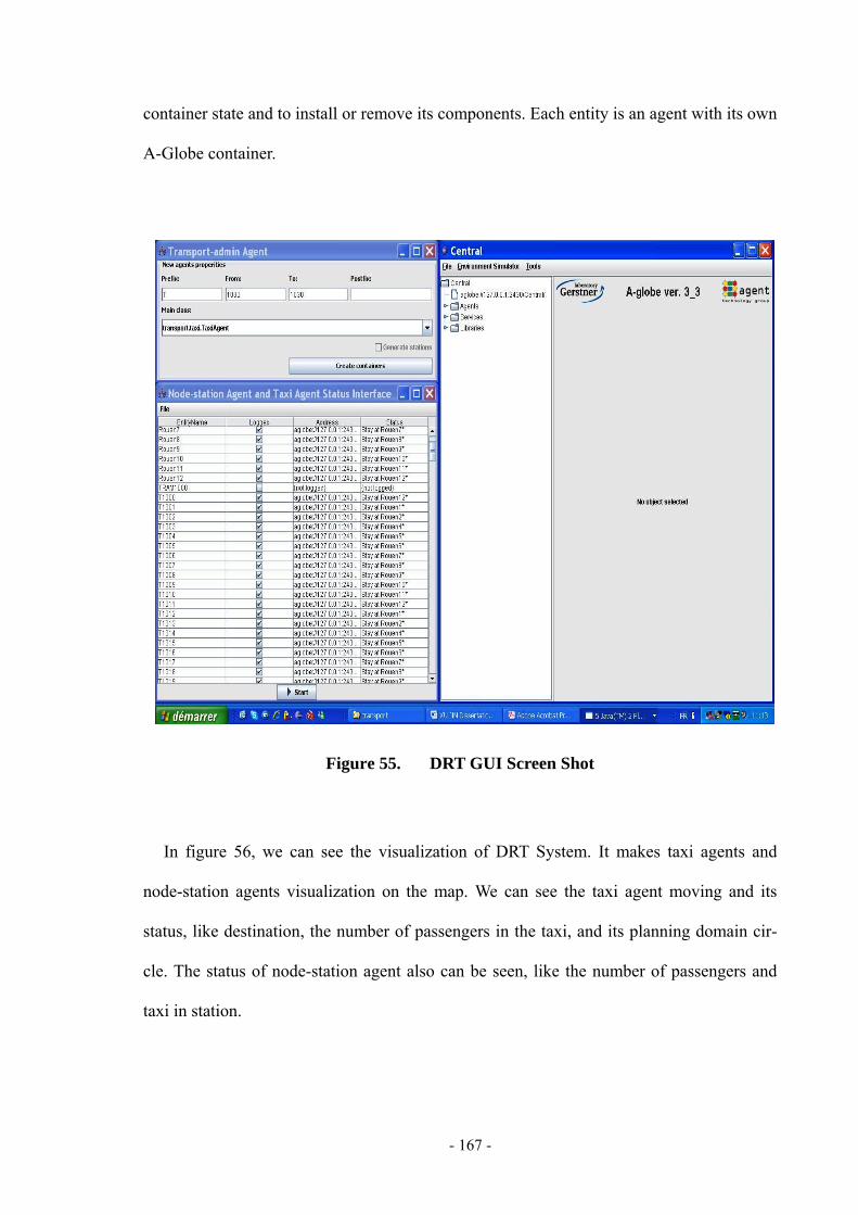
- 167 -

container state and to install or remove its components. Each entity is an agent with its own

A-Globe container.

Figure 55. DRT GUI Screen Shot

In figure 56, we can see the visualization of DRT System. It makes taxi agents and

node-station agents visualization on the map. We can see the taxi agent moving and its

status, like destination, the number of passengers in the taxi, and its planning domain cir-

cle. The status of node-station agent also can be seen, like the number of passengers and

taxi in station.

- 168 -

Figure 56. Visualization of DRT System

If double click the entity name on the Node-station and Taxi agent Status interface, we

can see the single taxi agent status interface (see Figure 57). Capacity and actual status

can be seen in the interface.

By the same way, we can open single node-station agent status interface (see Figure 58).

The waiting passenger’s information in the station can be seen in interface.

- 169 -

Figure 57. Single Taxi Agent Status Interface

Figure 58. Single Node-Station Agent Status Interface

- 170 -

6.3 Experiments Analysis

6.3.1 Structure of Experiments

In last sections, we introduced the planning domain based plan merging algorithm and

prototype the implementation. In this section the experimental will be discussed.

For the performance of the plan merging algorithm, we are interested in the realistic as-

pects. For example, to find minim number of taxis for trip requests, increase the efficient

passages in every vehicle, and while at the same time reduce the number of vehicles on the street

for reducing the air pollution caused by the vehicle, traffic congestion and financial cost.

The ideal data set to use for these experiments would consist of the schedules of several

trip requests and taxis in the one region and for the same time passages and taxis are pre-

pared to share taxis. The experiment is organized as follows: The test considered 500

random trips requests in one hour, the capacity of the vehicle (total number of seats) is 4.

The scenario has 12 stations. These plans were merged using the plan merging algorithm in

taxi agent planning domain. We assume that we constructed an action resource plan for

each of the taxi agent at first, and the taxi agents try to improve their plans using the plan-

ning domain based plan merging algorithm.

We assume that taxi agent can exchange information in its planning domain. Therefore,

our goal is to reduce the costs by taxi agents exchanging their resource among taxi agents

in its planning domain and planning together. The attributes of resource describes a taxi

agent like agent ID, destination station, the number of useable seat, preferred pickup time,

agents who get in and get out of its planning domain, etc. The most important resource

facts for plan merging in planning domain are the ride of a taxi that passengers to travel

from one location to another and agent’s ID who get in and get out of its planning domain.

- 171 -

6.3.2 Experiment and Results Analyze

The scenario of the test considered 500 random trips requests in one hour, the capacity

of the vehicle (total number of seats) is 4. The scenario has 12 stations, we set taxi (taxi

agent) number as 30, 40, 50, 60, 70. At first, we set each taxi agent has a limited planning

domain as introduced that in one taxi agent planning domain there will not have two sta-

tion-agents. The results (see Figure 59) show the number of waiting passengers depending

on number of taxis. The approach gives better results for the clients, which provides an ac-

ceptable balance between cost, and service quality. In figure 59, we can see that there are

will no passenger waiting if 60 taxis in the street. And there are will have almost five pas-

sengers waiting if 50 taxis in the street. So in this scenario, it is necessary 50 taxis spread

into all stations.

Number of taxis

30 40 50 60 70

Num

ber o

f wai

ting

pass

enge

rs

0

10

20

30

40

50

Col 2

Figure 59. Simulation Result with Limited Planning Domain

- 172 -

Then we set each taxi agent has an unlimited planning domain that it can communicate

with all other agents. The results (see Figure 60) show the number of waiting passengers

depending on number of taxis. So in this scenario, it is necessary 70 taxis spread into all

stations. In figure 61, we have compared the two results. The model with the limited plan-

ning domain is more effectively than unlimited. On the other hand, we can see the multi-

layer distributed hybrid planning model performs better from the vehicles’ perspective.

Number of taxis

30 40 50 60 70

Num

ber o

f wai

ting

pass

enge

rs

0

10

20

30

40

50

60

70

Col 2

Figure 60. Simulation Result with Unlimited Planning Domain

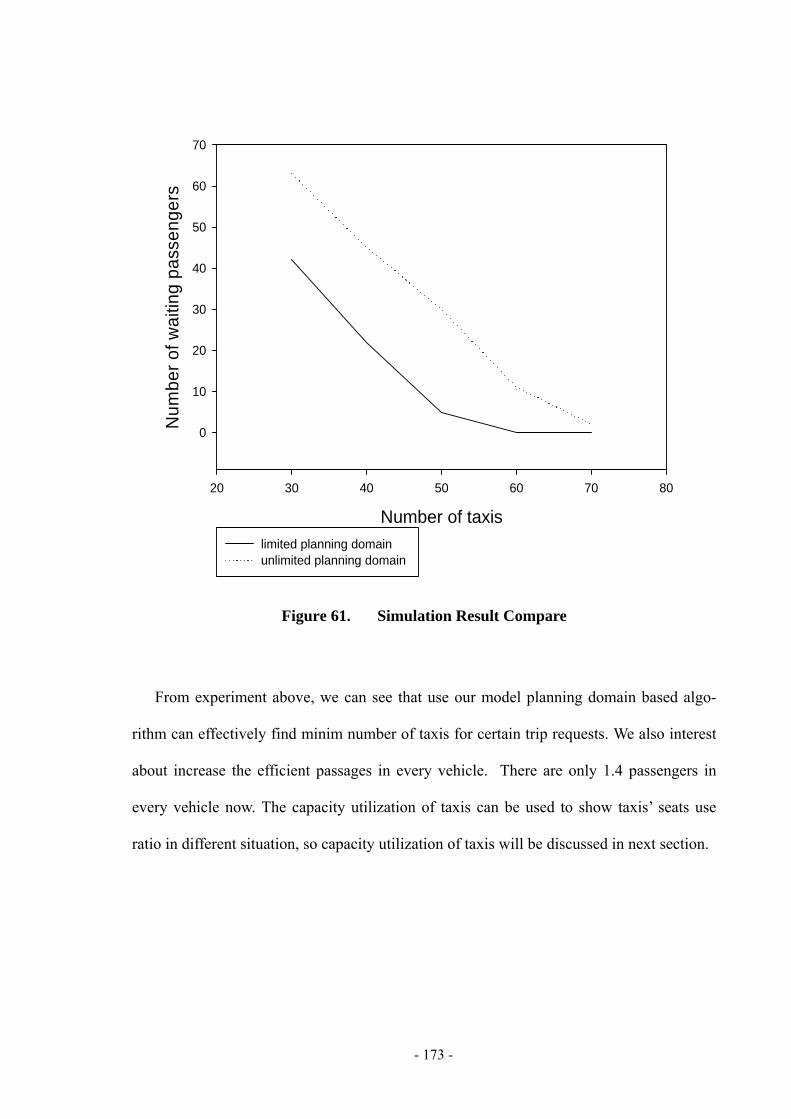
- 173 -

Number of taxis

20 30 40 50 60 70 80

Num

ber o

f wai

ting

pass

enge

rs

0

10

20

30

40

50

60

70

limited planning domainunlimited planning domain

Figure 61. Simulation Result Compare

From experiment above, we can see that use our model planning domain based algo-

rithm can effectively find minim number of taxis for certain trip requests. We also interest

about increase the efficient passages in every vehicle. There are only 1.4 passengers in

every vehicle now. The capacity utilization of taxis can be used to show taxis’ seats use

ratio in different situation, so capacity utilization of taxis will be discussed in next section.

- 174 -

65

70

75

80

85

90

95

100

105

0

10

2030

4050

2030

4050

6070

Cap

acity

util

izat

ion

of ta

xis

(%)

Numbe

r of w

aitin

g pa

ssen

gers

Number of taxis

Col 2 vs Col 1 vs Col 3

Figure 62. Capacity Utilization of Taxis with Limited Planning Domain

In the figure 62, it shows the relationship among capacity utilization of taxis, number of

taxis and number of waiting passengers in planning domain limited situation. We can see

that when there are 30 taxis (taxi agents) in the street, the capacity utilization of taxis is

almost 99%, but there are 42 passengers waiting. If there are 70 taxis (taxi agents) in the

street, there are no passengers waiting, but the capacity utilization of taxis is only 68%. So

we can see 50 taxis in the street is the best result, because it has a balance among capacity

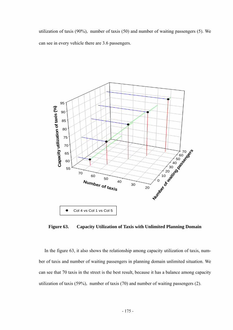
- 175 -

utilization of taxis (90%), number of taxis (50) and number of waiting passengers (5). We

can see in every vehicle there are 3.6 passengers.

55

60

65

70

75

80

85

90

95

010

2030

4050

6070

2030

4050

6070

Cap

acity

util

izat

ion

of ta

xis

(%)

Num

ber o

f wait

ing

pass

enge

rs

Number of taxis

Col 4 vs Col 1 vs Col 5

Figure 63. Capacity Utilization of Taxis with Unlimited Planning Domain

In the figure 63, it also shows the relationship among capacity utilization of taxis, num-

ber of taxis and number of waiting passengers in planning domain unlimited situation. We

can see that 70 taxis in the street is the best result, because it has a balance among capacity

utilization of taxis (59%), number of taxis (70) and number of waiting passengers (2).

- 176 -

Number of taxis

30 40 50 60 70

Cap

acity

util

izat

ion

of ta

xis

(%)

0

20

40

60

80

100

120

limited planning domainunlimited planning domain

Figure 64. Capacity Utilization of Taxis Result Compare

In figure 64, we have compared the results of capacity utilization of taxis. It shows that

the model with the limited planning domain is evidently more effectively than unlimited in

the same number of taxis (taxi agents) in the street. So we can see that the multi-layer dis-

tributed hybrid planning model performs better from the vehicles’ seats use ratio

perspective.

- 177 -

Chapter 7. Conclusion and Future Work

7.1 Conclusion

In recent years, more and more people care about urban traffic congestion and air pollu-

tion problems of many cities in the world. In order to reduce congestion, we can invest in

improving city infrastructures. Infrastructure improvements, however, are very costly to

undertake and do not reduce air pollution. Hence we can work on the intelligent mobility in

order to have a more efficient car use. The application of new information technologies,

such as multi-agent technologies to urban traffic information control, has made it possible

to create and deploy more intelligent traffic management like DRT (Demand Responsive

Transport) system. The objective of multi-agent based DRT system is to manage taxis in an

intelligent way, to increase the efficient number of passengers in every vehicle, and at the

same time to decrease the number of vehicles on streets. This will reduce the CO2 emis-

sions and air pollution caused by the vehicles, as well as traffic congestion and financial

costs.

In this thesis we have:

• Discussed the background and relevant work on DRT (Demand Responsive

Transport) system.

• Discussed the theoretical foundation of multi-agent based simulation and DRT

system.

• Described a multi-agent architecture for the urban DRT intelligent control sys-

tem.

• Investigated various multi agent planning problems and approaches.

- 178 -

• Proposed a new multi-agent based multi-layer distributed hybrid planning

model for DRT system.

• Developed an efficient planning domain based plan merging algorithm. Ex-

periments on established benchmark sets show the validity of our approach.

The intent of this study is to develop a multi-agent based analytical modeling approach

as to demand responsive transport (DRT) simulation model. Unlike standard optimization

procedures that require the knowledge of the exact spatial and temporal location of the de-

mand points, we propose a methodology using spatial and temporal distribution of trip

demand. Our methodology makes effective solution for this distributed situation.







propose an agent based multi-layer distributed hybrid planning model for the real-time

problem which can solve this question. In the proposed method, an agent for each vehicle

finds a set of routes by its local search, and selects a route by cooperation with other agents

in its planning domain. By computational experiments, we examine the effectiveness of the

proposed method.

7.2 Future Work

This thesis attempted to find a multi-agent based method to solve demand responsive

transport (DRT) problem in urban real-time distributed situation. Our project “Gestion

- 179 -

Temps Réel du Transport Collectif à la Demande (CPER) Budgetthe French” will continue. Fur-

ther study include: improving multi-layer distributed hybrid planning model, doing more

experiments, developing application, and application to wider domain of problem.

Improving multi-layer distributed hybrid planning model

As mentioned above, in the multi-layer distributed hybrid planning model we have:

• A multi-layer distributed hybrid structure is used.

• The node-station agent applies filtering policies and communicates in real-time.

• The taxi agent makes proposals for the actual plan, process change information

with the node-station agent and other taxi agents in its planning domain, updates

the plan and reschedules the remaining requests, transport passengers.

New distributed planning domain based agent plan mechanisms and algorithms may

benefit from ideas like the exchange only of summary needed information, even if the in-

formation used in different planning domain. The point is here: the node-station agent

abstract relevant information what needed by other node-station agents in its involved

planning domain. So in this way we can reduce communication costs and improves pri-

vacy and communications competence and taxi agent can update his plan more quickly and

more efficient.

Application to wider domain of problem

The multi-agent system is an autonomous intelligent computer system, in which every

agent always has a certain level of intelligence. The level of an agent’s intelligence could

vary from having pre-determined roles and responsibilities to a learning entity. A multi-

- 180 -

agent system is an aggregate of agents, with the objective of decomposing a larger system

into several smaller agent systems in which they communicate and cooperate with one

other. So agent-based model can produce high-quality simulations for complex and large-

scale real-time distributed system behaviors, like the urban traffic system that a large-scale

complex system with multiple entities and complicated relationships among them.

In real world, there are many different real-time distributed systems like DRT system.

So our multi-layer distributed hybrid planning model also can apply to these systems. For

example, like aviation system. In aviation system, the airport in every city cannot move

like node-station in DRT system, the plane transport passengers among different airports in

different cities like taxi. How to make the plane usage more efficient by change passen-

ger’s trip information is a problem. Certainly one plane do not need to communicate and

change information with all other planes in the world. Our model can be extended apply to

this problem.

And for supermarket supplies distribution system, every supermarket in the city cannot

move like node-station, the truck transport different supplies request for different super-

market like taxi. By change the supplies request information, how to make the trucks usage

more efficient and quickly, and at the same time to reduce the cost of transport is a prob-

lem. Our model also can be extended apply to this problem.

So as future work is considered to continue optimizing our model with known bench-

marks and extend its application.

- 181 -

References

[1] P. Bakker, "Large scale demand responsive transit systems –A local suburban trans-

port solution for the next millennium," AVV Transport Research Centre, Ministry of

Transport, Public Works and Water Management, Rotterdam, Netherlands 1999.

[2] R. E. Lave, Teal, R. and Piras, P., "A handbook for acquiring demand-responsive

transit software," Transportation Research Board, Washington, D.C 1996.

[3] K. Palmer, Dessouky, M. M., and Abdelmaguid, "Impacts of management practices

and advanced technologies on demand responsive transit systems " Transportation Re-

search, Part A: Policy and Practice, vol. 38, pp. 495-509, 2004.

[4] M. W. P. a. S. Savelsbergh, M, "The general pickup and delivery problem," Trans-

portation Science, vol. 29, pp. 17-29, 1995.

[5] G. Desaulniers, Desrosiers, J., Erdmann, A., Solomon, M.M. and Soumis, F., "The

VRP with pickup and delivery," Philadelphia 2001.

[6] F. Robusté, Daganzo, C.F. and Souleyrette, R.R., "Implementing vehicle routing

models," Transportation Research B, vol. 24B, pp. 263-286, 1990.

[7] J. M. Del Castillo, "A heuristic for the traveling salesman problem based on a con-

tinuous approximation," Transportation Research B, vol. 33B, pp. 123-152, 1999.

[8] J. D. Nelson, "Recent developments in telematics-based demand responsive trans-

port," in Presented at the IVT seminar University of Newcastle upon Tyne, 2003.

[9] J. Brake and J. D. Nelson, "A case study of flexible solutions to transport demand

in a deregulated environment," Journal of Transport Geography, vol. 15, pp. 262-273,

2007.

- 182 -

[10] " MobiSoft website www.mobisoft.com."

[11] "PersonalBus website http://www.personalbus.it/."

[12] M. Horn, "Fleet scheduling and dispatching for demand responsive passenger ser-

vices," Transportation Research Part C, vol. 10, pp. 35-63, 2002.

[13] M. Horn, "Modelling and assessment of demand-responsive passenger transport

services," in Applied GIS and Spatial Analysis, J. S. a. G. Clarke, Ed. Chichester: Wiley,

2003.

[14] "Analysis of User Needs for Demand Responsive Transport Services," 1996.

[15] "Logical Transport website http://www.logicaltransport.com/drt/index.html."

[16] D. Lee, "Requiem for large-scale models," 1975.

[17] I. Benenson, Torrens, P., Geosimulation: Automata-based modeling of urban phe-

nomena: John Wiley & Sons Ltd, 2004.

[18] T. Garaix, C. Artigues, D. Feillet, and D. Josselin, "Vehicle routing problems with

alternative paths: an application to on-demand transportation," HAL - CCSD, 2008.

[19] N. P. Russell S. , Artificial Intelligence: A Modern Approach. Upper Saddle River,

N.J., Great Britain, 2003.

[20] C. E., Transportation Systems Engineering: Theory and Methods: Kluwer Aca-

demic Press, 2001.

[21] M. B., Intelligent transportation systems architecture Artech House Books, 1999.

[22] L. J. M. R. Partich A.M.Ehlert, "Microscopic traffic simulation with reactive driv-

ing agents," in Proceedings of the IEEE Intelligent Transportation Systems Conference,

Oakland, USA, 2001, pp. 860-865.

- 183 -

[23] A. A. S. N. F. J. Miguel Leitao, "Graphical Control of Autonomous Virtual Vehi-

cles," in Proceedings of the IEEE Vehicular Technology Conference, Tokyo, Japan, 2000,

pp. 507-511.

[24] M. S. Joacbim Wahle, "A Multi-Agent System for On-lie Simulations based on

Real-World Traffic Data," in Proceedings of the International Conference on System Sci-

ences Hawaii,USA, 2001, pp. 1125-1133.

[25] K. Nagel, Traffic Networks. Weinheim, Germany: Wiley - VCH, 2003.

[26] F. C. Guidi-Polanco, C., "Architecting Global Automation Systems over a Distrib-

uted Multi-agent Infrastructure," in Software Architecture: 2nd European Workshop Berlin:

Springer, 2005, pp. 18-29.

[27] M. Wooldridge and N. R. Jennings, "Intelligent Agents: Theory and Practice," The

Knowledge Engineering Review, vol. 10, pp. 115-152, 1995.

[28] L. H. S. Green, B. Nangle, P. Cunnigham, F. Somers and R. Evans, "Software

Agents: A Review," Trinity College Dublin1 Broadcom E'ireann Research Ltd.2, 1997.

[29] R. D. B. J. Grosz, "AAAI Report to ARPA on 21st Century Intelligent Systems," AI

Magazine, pp. 10-20, 1994.

[30] O. M. Group, "Agent Platform Special Interest Group. Agent Technology," 2000.

[31] R. A. Brooks, "A robust layered control system for a mobile robot," IEEE Transac-

tions on Robotics and Automation, vol. 2(1), pp. 14-23, 1986.

[32] M. J. Matarić, "Interaction and Intelligent Behaviour," MIT, 1994.

[33] K. S. N. R. Jennings, M. Wooldridge, "A Roadmap of Agent Research and Devel-

opment," Autonomous Agents and Multi-Agent Systems 1, pp. 275-306, 1988.

- 184 -

[34] R. A. Brooks, "A Robot That Walks: Emergent Behaviour from a Carefully Evolved

Network," Neural Computation 1, pp. 153-162, 1989.

[35] I. A. Ferguson, "Touring Machines: An Architecture for Dynamic, Rational, Mobile

Agents." vol. PhD thesis: University of Cambridge, 1992.

[36] G. N. Boone, "Efficient Reinforcement Learning: Model-Based Acrob ot Control,"

in IEEE International Conference on Robotics and Automation Albuquerque, 1997, pp.

229-234.

[37] L. H. S. Green, B. Nangle, P. Cunnigham, F. Somers and R. Evans, "Software

Agents: A Review " Trinity College Dublin1 Broadcom E'ireann Research Ltd.2, 1997.

[38] N. R. Jennings, K. Sycara, and M. Wooldridge, "A Roadmap of Agent Research and

Development," Autonomous Agents and Multi-Agent Systems 1, pp. 275-306, 1998.

[39] H. S. Nwana, "Software Agents: An Overview," Knowledge Engineering Review,

vol. 11(3), pp. 1-40, 1996.

[40] A. Newell and H. A. Simon, "Computer Science as Empirical Enquiry," Communi-

cations of the ACM 19, pp. 113-126, 1976.

[41] R. Fikes and N. Nilsson, "STRIPS: A New Approach to the Application of Theorem

Proving to Problem Solving," Artificial Intelligence, vol. 2 (3), pp. 189-208, 1971.

[42] A. Newell and H. A. Simon, "GPS, a Program That Simulates Human Thought," in

Computers and Thought USA: MIT Press, 1995, pp. 279-293.

[43] A. A. Perez-Uribe and B. Hirsbrunner, Learning and Foraging in Robot-bees.

Honolulu: International Society for Adaptive Behavior, 2000.

- 185 -

[44] R. Aylett, R. A. Ghanea-Hercock, and A. M. Coddington, "Supervising multiple co-

operating mobile robots," in Proceedings of the first international conference on

Autonomous agents, California, United States, 1997, pp. 514-515.

[45] P. Maes, "The Agent Network Architecture (ANA)," 1991.

[46] A. H. Bond and L. Gasser, An Analysis of Problems and Research in DAI. San

Mateo CA: Morgan Kaufmann Publishers, 1988.

[47] J. S. Rosenschein and G. Zlotkin, Rules of encounter: designing conventions for

automated negotiation among computers: MIT Press, 1994.

[48] R. A. Brooks, "Intelligence Without Representation," Artificial Intelligence Journal

47, pp. 139–159, 1991.

[49] G. Weiss, Multiagent Systems: A Modern Approach to Distributed Artificial Intelli-

gence. Massachusetts, USA: MIT Press, 1999.

[50] C. W. Reynolds, "Flocks, herds, and schools: A distributed behavioral model,"

Computer Graphics, vol. 21(4), pp. 25-34, 1987.

[51] P. Davidsson, "Multi Agent Based Simulation: Beyond social simulation," in Multi

Agent Based Simulation, S. Moss and P. Davidsson, Eds.: Springer-Verlag, 2000.

[52] H. V. D. Parunak, "Go to the Ant': Engineering Principles from Natural Agent Sys-

tems," Annals of Operations Research, vol. 75, pp. 69-101, 1997.

[53] M. W. Macy and R. Willer, "From factors to actors: computational sociology and

agent-based modeling," Annual Review of Sociology, vol. 28, pp. 143-166, 2002.

[54] H. J. Scholl, "Agent-based and System Dynamics Modeling: A Call for Cross Study

and Joint Research," in Proceedings of 34th Annual Hawaii International Conference on

System Sciences ( HICSS-34), Maui, Hawaii, USA, 2001, p. 8.

- 186 -

[55] R. Hammond, "Simplified Worlds and Macroscopes: The Power of Agent-Based

Modeling," 2003.

[56] N. Gilbert and P. Terna, "How to build and use agent-based models in social sci-

ence," Mind & Society, vol. 1, pp. 55-72, 2000.

[57] R. Axelrod, The Complexity of Cooperation: Agent-Based Models of Competition

and Collaboration. Princeton, NJ: Princeton University Press, 1997.

[58] L. Hood, "Agent based modelling," 2002.

[59] P. A. Fishwick, J. G. Sanderson, and W. F. Wolff, "A multimodeling basis for

acrosstrophic- �level ecosystem modeling: The orida everglades example," Transactions of

the Society for Computer Simulation, vol. 15(2), pp. 76-89, 1998.

[60] G. Hartvigsen and S. Levin, "Evolution and spatial structure interact to influence

plant-herbivore population and community dynamics," in Proceedings of the Royal Society

of London, 1997, pp. 1677-1685.

[61] D. J. T. Sumpter, "From Bee to Society: An Agent-based Investigation of Honey

Bee Colonies." vol. PhD Manchester, United Kingdom: University of Manchester, 2000.

[62] M. e. a. Scheffer, "Super-individuals: a simple solution for modelling large popula-

tions on an individual basis," Ecological Modelling, vol. 80(2-3), pp. 161-170, 1995.

[63] D. H. e. a. Deutschman, "Scaling from trees to forests: Analysis of a complex simu-

lation model," Science, vol. 277, 1997.

[64] B. McMullin and F. J. Varela, "Rediscovering computational autopoiesis," in

`Fourth European Conference on Artificial Life, P. Husbands and I. Harvey, Eds. Brington,

UK: MIT Press, 1997.

- 187 -

[65] N. Basu, R. Pryor, T. Quint, and T. Arnold, "Aspen: A microsimulation model of the

economy," Sandia National Laboratories, Albuquerque, NM 1996.

[66] M. e. a. Raberto, "Agent-based simulation of a financial market," Physica A: Statis-

tical Mechanics and its Applications, vol. 299(1-2), pp. 319-327, 2001.

[67] L. Tesfatsion, "Agent-based computational economics: Growing economies from

the bottom-up," Artificial Life, vol. 8(1), pp. 55-82, 2002.

[68] R. Chakrabarti, "An agent based model of corruption," Georgia Institute of Tech-

nology 2002.

[69] C. McPhail, Stereotypes of crowds and collective behavior: Looking backward,

looking forward. Greenwich, CT: JAI Press Inc., 1997.

[70] D. Helbing, I. Farkas, and T. Vicsek, "Simulating dynamical features of escaping

panic," Nature 407, pp. 487-490, 2000.

[71] I. Benenson and I. Omer, "Agent-based modeling of residential distribution," De-

partment of Geography and Human Environment, University Tel Aviv, Israel 2001.

[72] J. J. Merelo, A. Prieto, and V. Rivas, "An agent based model for the study of public-

ity/consumer dynamics," in Fourth European Conference on Artificial Life, P. Husbands

and I. Harvey, Eds. Brington, UK: MIT Press, 1997.

[73] D. L. Lauen, "An Agent Based Modeling Approach to School Choice," in Proceed-

ings of Annual Meeting of the American Sociological Association, 2003.

[74] L. Gulyás, B. Adamcsek, and Á. Kiss, "Experimental Economics Meets Agent-

Based Finance: A Participatory Artificial Stock Market," in Proceedings of 34th Annual

Conference of International Simulation and Gaming Association (ISAGA 2003), 2003.

- 188 -

[75] E. Bonabeau, "Agent-based modeling: Methods and techniques for simulating hu-

man systems," in PNAS 99, 2002, pp. 7280-7287.

[76] A. Kanafani, Transportation Demand Analysis. New York: McGraw-Hill, 1983.

[77] P. S. McCarthy, Transportation Economics: Theory and Practice: A Case Study Ap-

proach. Malden, MA: Blackwell pub., 2001.

[78] M. Labb´e and e. al., "Operations Research and Decision Aid Methodologies in

Traffic and Transportation Management." vol. 166 Berlin, Germany: Springer-Verlag,

1998.

[79] R. B. Noland, "Relationship between highway capacity and induced vehicle travel,"

Transprotation Research Part A pp. 47-72, 2001.

[80] R. Huang, "Some inequalities for the Hadamard product and the Fan product of ma-

trices," Linear Algebra and its Applications vol. 428, pp. 1551-1559, 2008.

[81] B. B. White, "Empirical tests of the life cycle hypothesis," The American Economic

Review, vol. 68(4), pp. 547-560, 1978.

[82] A. G. Wilson, "A statistical theory of spatial distribution models," Transportation

Research Part B 1, pp. 253-269, 1967.

[83] M. Bierlaire, "Mathematical Models for Transportation Demand Analysis." vol.

PhD Namur, Belgium: Facultés Universitaires Notre-Dame de la Paix, 1996.

[84] D. E. Smith and D. S. Weld, "Temporal planning with mutual exclusion reasoning,"

in Proceedings of the Sixteenth International Joint Conference on Artificial Intelligence

(IJCAI-99), San Mateo, CA, 1999.

[85] S. Kambhampati, "Refinement planning as a unifying framework for plan synthe-

sis," AI Magazine, vol. 18(2), pp. 67-97, 1997.

- 189 -

[86] D. S. Weld, "An introduction to least-commitment planning," AI Magazine, vol.

15(4), pp. 27-61, 1994.

[87] R. Korf, "Planning as search: A quantitative approach," Artificial Intelligence, vol.

33(1), pp. 65-88, 1987.

[88] S. Russell and P. Norvig, Artificial Intelligence: A Modern Approach: Prentice Hall,

1995.

[89] A. Newell and H. A. Simon, GPS, a program that simulates human thought, 1969.

[90] E. P. D. Pednault, "Formulating multi-agent dynamic-world problems in the classi-

cal planning framework," in Reasoning About Actions and Plans: Proceedings of the 1986

Workshop, M. P. Georgeff and A. L. Lansky, Eds. San Mateo, CA: Morgan Kaufmann Pub-

lishers, 1987, pp. 47-82.

[91] M. Fox and D. Long, "Pddl2.1: An extension of pddl for expressing temporal plan-

ning domains," Journal of AI Research, vol. 20, pp. 61-124, 2003.

[92] M. Brenner, "Multiagent planning with partially ordered temporal plans," in Pro-

ceedings of the Doctorial Consortium of the International Conferenence on AI Planning

and Scheduling, 2003.

[93] M. P. Georgeff, "Communication and interaction in multi-agent planning," in Pro-

ceedings of the Third National Conference on Artificial Intelligence (AAAI-83), Menlo

Park, CA, 1983, pp. 125-129.

[94] M. Ghallab, D. Nau, and P. Traverso, Automated Planning: Theory and Practice:

Morgan Kaufmann, 2004.

[95] A. L. Blum and M. L. Furst., "Fast planning through planning graph analysis," Arti-

ficial Intelligence, vol. 90, pp. 281-300, 1997.

- 190 -

[96] D. S. Weld, "Recent advances in AI planning," AI Magazine, vol. 20(2), pp. 93-123,

1999.

[97] B. Srivastava, S. Kambhampati, and M. B. Do, "Planning the project management

way: Efficient planning by effective integration of causal and resource reasoning in

RealPlan," Artificial Intelligence, vol. 131(1-2), pp. 73-134, 2001.

[98] F. Bacchus and F. Kabanza, "Using temporal logics to express search control

knowledge for planning," Artificial Intelligence, vol. 116, pp. 123-191, 2000.

[99] J. Hoffmann and B. Nebel, "The FF planning system: Fast plan generation through

heuristic search," Journal of AI Research, vol. 14, pp. 253-302, 2001.

[100] D. Marr, Vision: Freeman Publishers, 1982.

[101] J. S. Penberthy and D. S. Weld., "UCPOP: A sound, complete, partial order planner

for ADL," in Proceedings of the Third International Conference on Knowledge Representa-

tion and Reasoning (KR&R-92), 1992, pp. 103-114.

[102] E. Schwalb and L. Vila, "Temporal constraints: A survey," Constraints: An Interna-

tional Journal of AI Research, vol. 3(2/3), pp. 129-149, 1998.

[103] R. Dechter, I. Meiri, and J. Pearl, "Temporal constraint networks," Artif. Intell., vol.

49(1-3), pp. 61-95, 1991.

[104] D. McAllester and D. Rosenblitt, "Systematic nonlinear planning," in Proceedings

of the Ninth National Conference on Artificial Intelligence, Anaheim, CA, 1991, pp. 634-

639.

[105] D. Chapman, "Planning for conjunctive goals," Artificial Intelligence, vol. 32, pp.

333-377, 1987.

- 191 -

[106] J. S. Penberthy and D. S. Weld, "Temporal planning with continuous change," in

Proceedings of the Twelfth National Conference on Artificial Intelligence (AAAI-94),

Menlo Park, CA, 1994, pp. 1010-1015.

[107] A. Tate, "Generating project networks," in Proceedings of the Fifth International

Joint Conference on Artificial Intelligence, 1977, pp. 888-893.

[108] E. D. Sacerdoti, "The nonlinear nature of plans," in Proceedings of the Fourth In-

ternational Joint Conference on Artificial Intelligence, 1975, pp. 206-214.

[109] D. Nau, Y. Cao, A. Lotem, and H. M. n. Avila., "SHOP: A Simple Hierarchical Or-

dered Planner," in Proceedings of the Sixteenth International Joint Conference on Artificial

Intelligence, 1999.

[110] D. Nau, T.-C. Au, O. Ilghami, U. Kuter, J. W. Murdock, DanWu, and F. Yaman,

"SHOP2: An HTN planning system," Journal of Artificial Intelligence Research, vol. 20,

pp. 379-404, 2003.

[111] R. Tsuneto, J. A. Hendler, and D. S. Nau, "Analyzing external conditions to im-

prove the efficiency of HTN planning," in Proceedings of the Fifteenth National

Conference on Artificial Intelligence (AAAI-98), Menlo Park, CA, 1998.

[112] B. J. Clement and E. H. Durfee, "Top-down search for coordinating the hierarchical

plans or multiple agents," in Proceedings of the Third International Conference on

Autonomous Agents(Agents’99), Seattle, WA, USA, 1999.

[113] G. Zlotkin and J. S. Rosenschein, "Mechanisms for automated negotiation in state

oriented domains," Journal of Artificial Intelligence Research, vol. 5, pp. 163-238, 1996.

[114] M. Browning, B. Browning, and M. Veloso, "Plays as effective multiagent plans

enabling opponent-adaptive play selection," in Proceedings of the Fourteenth International

Conference on Automated Planning and Scheduling,, Vancouver, 2004.

- 192 -

[115] K. Biggers and T. Ioerger, "Automatic generation of communication and teamwork

within multi-agent teams," Applied Artificial Intelligence, vol. 15, pp. 875-916, 2001.

[116] M. M. d. Weerdt and R. P. J. v. d. Krogt, "A method to integrate planning and coor-

dination," Menlo Park, CA 2002.

[117] D. E. Wilkins and K. L. Myers, "A Multiagent Planning Architecture," in Proceed-

ings of the Fourth International Conference on Artificial Intelligence Planning Systems

(AIPS-98), Menlo Park, CA, 1998, pp. 154-162.

[118] M. Yokoo and K. Hirayama., "Algorithms for distributed constraint satisfaction: A

review of ”plans and situated actions” by Lucy Suchman," Autonomous Agents and Multi-

Agent Systems, 2000.

[119] N. R. Jennings, "Commitments and conventions: The foundation of coordination in

multiagent systems," The Knowledge Engineering Review, vol. 8(3), pp. 223-250, 1993.

[120] K. S. Decker and V. R. Lesser, "Generalizing the Partial Global Planning algo-

rithm," International Journal of Intelligent and Cooperative Information Systems, vol. 1(2),

pp. 319-346, 1992.

[121] B. Horling, V. Lesser, R. Vincent, T. Wagner, A. Raja, S. Zhang, K. Decker, and A.

Garvey, "The TAEMS white paper," 1999.

[122] M. E. desJardins, E. H. Durfee, C. L. O. Jr., and M. J. Wolverton., "A survey of re-

search in Distributed, Continual Planning," AI Magazine, 2000.

[123] R. Alami, F. Ingrand, and S. Qutub, "A scheme for coordinating multi-robot plan-

ning activities and plans execution," in Proceedings of the Thirteenth European Conference

on Artificial Intelligence, Brighton, UK, 1998.

- 193 -

[124] I. Tsamardinos, M. E. Pollack, and J. F. Horty, "Merging plans with quantitative

temporal constraints, temporally extended actions, and conditional branches," in Proceed-

ings of the Fifth International Conference on Artificial Intelligence Planning Systems

(AIPS-00), Menlo Park, CA, 2000, pp. 264-272.

[125] M. M. d. Weerdt, R. P. J. v. d. Krogt, and C. Witteveen, "Resource Based Multi

Agent Plan Merging: framework and application," in Proceedings of the 22nd Annual

Workshop of the UK Planning and Scheduling Special Interest Group (PlanSIG-03), 2003.

[126] J. M. Valk, M. M. d. Weerdt, and C. Witteveen., Algorithms for coordination in

multi-agent planning. London: Idea Group Publishing, 2005.

[127] Q. Yang, D. S. Nau, and J. Hendler, "Merging separately generated plans with re-

stricted interactions," Computational Intelligence, vol. 8(4), pp. 648-676, 1992.

[128] Y. Shoham and M. Tennenholtz, "On social laws for artificial agent societies: Off-

line design," Artificial Intelligence, vol. 73(1–2), pp. 231-252, 1995.

[129] W. Briggs and D. J. Cook, "Modularity and Communication in Multi-Agent Plan-

ning." vol. PhD: University of Texas at Arlington, 1996.

[130] "A-Globe: A-Globe Agent Platform website http://agents.felk.cvut.cz/aglobe."

[131] L. Xiac-Ming and W. Fei-Yue, "Study of City Area Traffic Coordination Control on

The Basis of Agent," in Proceedings of the IEEE Intelligent Transportation Systems Con-

ference, Singapore, 2002, pp. 758-761.

[132] "Transportation Research Board," in Highway Capacity Manual, 2000.

[133] V. R. e. a. Tomás, "New technologies to work with traffic management plans," Traf-

fic Technology International-Annual review, 2003.

- 194 -

[134] W. H. Zhang Jin, Li Ping, "Towards the Applications of Multiagent Techniques in

Intelligent Transportation Systems," in Proceedings of the IEEE Int. Conf. on Intelligent

Transportation Systems, 2003, pp. 1750-1754.

[135] R. A. Alan B. Tickle, Mostefa Golea, and Joachim Diederich, "The truth will come

to light: Directions and challenges in extracting the knowledge embedded within trained

artificial neural networks," IEEE Transactions on Neural Networks, pp. 1057-1068, 1998.

[136] M. M. deWeerdt, A. Bos, J. Tonino, and C.Witteveen., "A resource logic for multi-

agent plan merging," Annals of Mathematics and A. I., special issue on Computational

Logic on Multi-Agent Systems, vol. 37(1–2), pp. 93-130, 2003.

[137] J. S. H. Yang, Y. H. Chin, and C. G. Chung, "Many-sorted first-order logic database

language," The Computer Journal vol. 35, pp. 129-137 1992.

[138] A. Serenko and B. Detlor, "Agent Toolkits: A General Overview of the Market and

an Assessment of Instructor Satisfaction With Utilizing Toolkits in the Classroom,"

McMaster University, Hamilton, Ontario 2002.

[139] P. Vrba, "Java-based agent platform evaluation," in Holonic and Multi-Agent Sys-

tems for Manufacturing, Marık, McFarlane, Valckenaers, and eds., Eds. Heidelberg:

Springer-Verlag, 2003, pp. 47-58.

- 195 -

- 196 -

Résumé Durant ces dernières années, la congestion du trafic urbain et la pollution de l'air sont devenus

d'énormes problèmes dans de nombreuses villes dans le monde. Afin de réduire cette congestion,

nous pouvons investir dans l'amélioration des infrastructures de la ville. Toutefois, cette solution

reste très coûteuse à entreprendre et de ne permet pas de réduire la pollution de l'air. C'est pourquoi

nous travaillons sur la mobilité intelligente afin de disposer d'une meilleure utilisation de la voiture.

L'application de nouvelles technologies de l'information, tels que les systèmes multi-agents

appliqués au contrôle de l'information de la circulation urbaine, a permis de créer et de déployer

une gestion plus intelligente du trafic comme le système DRT (transport à la demande). L'objectif

des systèmes multi-agents basés sur le DRT est de gérer les taxis de manière intelligente, afin

d'accroître le nombre de passagers dans chaque véhicule, et en même temps à réduire le nombre de

véhicules dans les rues. Cela permettra de réduire les émissions de CO2 et la pollution de l'air

causée par les véhicules, ainsi que la congestion du trafic et les coûts financiers associés.

La simulation multi-agents est considérée comme un outil efficace pour les services dynamiques

urbains de la circulation. Toutefois, le principal problème est de savoir comment construire un

agent à base de modèle pour cette problématique. Ces travaux de recherche présente une solution

basée sur les systèmes multi-agents réactifs pour la problématique du transport à la demande

(DRT), qui adopte une approche multi-agent de planification urbaine en utilisant des services de

contrôle qui satisfont aux principales contraintes : réduction de la période totale creuse, demandes

spéciales du client, augmentation du nombre de places utilisées dans un même taxi, utilisation du

nombre minimal de véhicules, etc. Dans cette thèse, nous proposons un modèle multi-agents

multicouche hybride distribué pour des problématiques en temps réel. Dans la méthode proposée,

un agent pour chaque véhicule trouve un ensemble de routes pour sa recherche locale, et choisit un

itinéraire en coopérant avec d'autres agents se trouvant dans son domaine de planification. Nous

avons examiné expérimentalement, l'efficacité de la méthode proposée.

Mots-clés: Systèmes multi-agents, Transport à la demande, Systèmes de transport intelligents.

a multi-agent based multi-layer distributed hybrid

Documents