a multi-model intercomparison of halogenated very … · 5department of chemistry, university of...
TRANSCRIPT

Atmos. Chem. Phys., 16, 9163–9187, 2016www.atmos-chem-phys.net/16/9163/2016/doi:10.5194/acp-16-9163-2016© Author(s) 2016. CC Attribution 3.0 License.
A multi-model intercomparison of halogenated very short-livedsubstances (TransCom-VSLS): linking oceanic emissions andtropospheric transport for a reconciled estimate of the stratosphericsource gas injection of bromineR. Hossaini1,a, P. K. Patra2, A. A. Leeson1,b, G. Krysztofiak3,c, N. L. Abraham4,5, S. J. Andrews6, A. T. Archibald4,J. Aschmann7, E. L. Atlas8, D. A. Belikov9,10,11, H. Bönisch12, L. J. Carpenter6, S. Dhomse1, M. Dorf13, A. Engel12,W. Feng1,4, S. Fuhlbrügge14, P. T. Griffiths5, N. R. P. Harris5, R. Hommel7, T. Keber12, K. Krüger14,15,S. T. Lennartz14, S. Maksyutov9, H. Mantle1, G. P. Mills16, B. Miller17, S. A. Montzka17, F. Moore17, M. A. Navarro8,D. E. Oram16, K. Pfeilsticker18, J. A. Pyle4,5, B. Quack14, A. D. Robinson5, E. Saikawa19,20, A. Saiz-Lopez21, S. Sala12,B.-M. Sinnhuber3, S. Taguchi22, S. Tegtmeier14, R. T. Lidster6, C. Wilson1,23, and F. Ziska14
1School of Earth and Environment, University of Leeds, Leeds, UK2Department of Environmental Geochemical Cycle Research, JAMSTEC, Yokohama, Japan3Institute for Meteorology and Climate Research, Karlsruhe Institute of Technology, Karlsruhe, Germany4National Centre for Atmospheric Science, Cambridge, UK5Department of Chemistry, University of Cambridge, Cambridge, UK6Department of Chemistry, University of York, Heslington, York, UK7Institute of Environmental Physics, University of Bremen, Bremen, Germany8Rosenstiel School of Marine and Atmospheric Science, University of Miami, Miami, USA9Center for Global Environmental Research, National Institute for Environmental Studies, Tsukuba, Japan10National Institute of Polar Research, Tokyo, Japan11Tomsk State University, Tomsk, Russia12Institute for Atmospheric and Environmental Sciences, Universität Frankfurt/Main, Frankfurt, Germany13Max-Planck-Institute for Chemistry, Mainz, Germany14GEOMAR Helmholtz Centre for Ocean Research Kiel, Kiel, Germany15University of Oslo, Department of Geosciences, Oslo, Norway16School of Environmental Sciences, University of East Anglia, Norwich, UK17National Oceanic and Atmospheric Administration, Boulder, USA18Institute for Environmental Physics, University of Heidelberg, Heidelberg, Germany19Department of Environmental Sciences, Emory University, Atlanta, USA20Department of Environmental Health, Rollins School of Public Health, Emory University, Atlanta, USA21Atmospheric Chemistry and Climate Group, Institute of Physical Chemistry Rocasolano, CSIC, Madrid, Spain22National Institute of Advanced Industrial Science and Technology, Tsukuba, Japan23National Centre for Earth Observation, Leeds, UKanow at: Lancaster Environment Centre, Lancaster University, Lancaster, UKbnow at: Lancaster Environment Centre/Data Science Institute, Lancaster University, Lancaster, UKcnow at: Laboratoire de Physique et Chimie de l’Environnement et de l’Espace, CNRS-Université d’Orléans, Orléans, France
Correspondence to: Ryan Hossaini ([email protected])
Received: 13 October 2015 – Published in Atmos. Chem. Phys. Discuss.: 18 January 2016Revised: 30 May 2016 – Accepted: 21 June 2016 – Published: 26 July 2016
Published by Copernicus Publications on behalf of the European Geosciences Union.
9164 R. Hossaini et al.: TransCom-VSLS Model Intercomparison Project
Abstract. The first concerted multi-model intercompari-son of halogenated very short-lived substances (VSLS) hasbeen performed, within the framework of the ongoing At-mospheric Tracer Transport Model Intercomparison Project(TransCom). Eleven global models or model variants partici-pated (nine chemical transport models and two chemistry–climate models) by simulating the major natural bromineVSLS, bromoform (CHBr3) and dibromomethane (CH2Br2),over a 20-year period (1993–2012). Except for three modelsimulations, all others were driven offline by (or nudged to)reanalysed meteorology. The overarching goal of TransCom-VSLS was to provide a reconciled model estimate of thestratospheric source gas injection (SGI) of bromine fromthese gases, to constrain the current measurement-derivedrange, and to investigate inter-model differences due to emis-sions and transport processes. Models ran with standardisedidealised chemistry, to isolate differences due to transport,and we investigated the sensitivity of results to a range ofVSLS emission inventories. Models were tested in their abil-ity to reproduce the observed seasonal and spatial distri-bution of VSLS at the surface, using measurements fromNOAA’s long-term global monitoring network, and in thetropical troposphere, using recent aircraft measurements –including high-altitude observations from the NASA GlobalHawk platform.
The models generally capture the observed seasonal cycleof surface CHBr3 and CH2Br2 well, with a strong model–measurement correlation (r ≥ 0.7) at most sites. In a givenmodel, the absolute model–measurement agreement at thesurface is highly sensitive to the choice of emissions. Largeinter-model differences are apparent when using the sameemission inventory, highlighting the challenges faced in eval-uating such inventories at the global scale. Across the ensem-ble, most consistency is found within the tropics where mostof the models (8 out of 11) achieve best agreement to sur-face CHBr3 observations using the lowest of the three CHBr3emission inventories tested (similarly, 8 out of 11 modelsfor CH2Br2). In general, the models reproduce observationsof CHBr3 and CH2Br2 obtained in the tropical tropopauselayer (TTL) at various locations throughout the Pacific well.Zonal variability in VSLS loading in the TTL is generallyconsistent among models, with CHBr3 (and to a lesser extentCH2Br2) most elevated over the tropical western Pacific dur-ing boreal winter. The models also indicate the Asian mon-soon during boreal summer to be an important pathway forVSLS reaching the stratosphere, though the strength of thissignal varies considerably among models.
We derive an ensemble climatological mean estimate ofthe stratospheric bromine SGI from CHBr3 and CH2Br2of 2.0 (1.2–2.5) ppt, ∼ 57 % larger than the best estimatefrom the most recent World Meteorological Organization(WMO) Ozone Assessment Report. We find no evidence fora long-term, transport-driven trend in the stratospheric SGIof bromine over the simulation period. The transport-driveninterannual variability in the annual mean bromine SGI is
of the order of ±5 %, with SGI exhibiting a strong positivecorrelation with the El Niño–Southern Oscillation (ENSO)in the eastern Pacific. Overall, our results do not show sys-tematic differences between models specific to the choice ofreanalysis meteorology, rather clear differences are seen re-lated to differences in the implementation of transport pro-cesses in the models.
1 Introduction
Halogenated very short-lived substances (VSLS) are gaseswith atmospheric lifetimes shorter than, or comparable to,tropospheric transport timescales (∼ 6 months or less atthe surface). Naturally emitted VSLS, such as bromoform(CHBr3), have marine sources and are produced by phyto-plankton (e.g. Quack and Wallace, 2003) and various speciesof seaweed (e.g. Carpenter and Liss, 2000) – a numberof which are farmed for commercial application (Leedhamet al., 2013). Once in the atmosphere, VSLS (and their degra-dation products) may ascend to the lower stratosphere (LS),where they contribute to the inorganic bromine (Bry) bud-get (e.g. Pfeilsticker et al., 2000; Sturges et al., 2000) andthereby enhance halogen-driven ozone (O3) loss (Salawitchet al., 2005; Feng et al., 2007; Sinnhuber et al., 2009; Sinnhu-ber and Meul, 2015). On a per molecule basis, O3 pertur-bations near the tropopause exert the largest radiative ef-fect (e.g. Lacis et al., 1990; Forster and Shine, 1997; Rieseet al., 2012), and recent work has highlighted the climate rel-evance of VSLS-driven O3 loss in this region (Hossaini et al.,2015a).
Quantifying the contribution of VSLS to stratospheric Bry(BrVSLS
y ) has been a major objective of numerous recent ob-servational studies (e.g. Dorf et al., 2008; Laube et al., 2008;Brinckmann et al., 2012; Sala et al., 2014; Wisher et al.,2014) and modelling efforts (e.g. Warwick et al., 2006; Hos-saini et al., 2010; Liang et al., 2010; Aschmann et al., 2011;Tegtmeier et al., 2012; Hossaini et al., 2012b, 2013; As-chmann and Sinnhuber, 2013; Fernandez et al., 2014). How-ever, despite a wealth of research, BrVSLS
y remains poorlyconstrained, with a current best-estimate range of 2–8 ppt re-ported in the most recent World Meteorological Organization(WMO) Ozone Assessment Report (Carpenter and Reimann,2014). Between 15 and 76 % of this supply comes from thestratospheric source gas injection (SGI) of VSLS, i.e. thetransport of a source gas (e.g. CHBr3) across the tropopause,followed by its breakdown and in situ release of BrVSLS
y
in the LS. The remainder comes from the troposphere-to-stratosphere transport of both organic and inorganic productgases, formed following the breakdown of VSLS below thetropopause; termed product gas injection (PGI).
Owing to their short tropospheric lifetimes, combined withsignificant spatial and temporal inhomogeneity in their emis-sions (e.g. Carpenter et al., 2005; Archer et al., 2007; Or-
Atmos. Chem. Phys., 16, 9163–9187, 2016 www.atmos-chem-phys.net/16/9163/2016/
R. Hossaini et al.: TransCom-VSLS Model Intercomparison Project 9165
likowska and Schulz-Bull, 2009; Ziska et al., 2013; Stemm-ler et al., 2015), the atmospheric abundance of VSLS canexhibit sharp tropospheric gradients. The stratospheric SGIof VSLS is expected to be most efficient in regions wherestrong uplift, such as convectively active regions, coincideswith regions of elevated surface mixing ratios (e.g. Tegt-meier et al., 2012, 2013; Liang et al., 2014), driven bystrong localised emissions or hotspots. Both the magnitudeand distribution of emissions, with respect to transport pro-cesses, could be, therefore, an important determining factorfor SGI. However, current global-scale emission inventoriesof CHBr3 and CH2Br2 are poorly constrained, owing to apaucity of observations used to derive their surface fluxes(Ashfold et al., 2014), contributing significant uncertainty tomodel estimates of BrVSLS
y (Hossaini et al., 2013). Given theuncertainties outlined above, it is unclear how well preferen-tial transport pathways of VSLS to the LS are represented inglobal-scale models.
Strong convective source regions, such as the tropicalwestern Pacific during boreal winter, are likely importantfor the troposphere-to-stratosphere transport of VSLS (e.g.Levine et al., 2007; Aschmann et al., 2009; Pisso et al.,2010; Hossaini et al., 2012b; Liang et al., 2014). The Asianmonsoon also represents an effective pathway for boundarylayer air to be rapidly transported to the LS (e.g. Randelet al., 2010; Vogel et al., 2014; Orbe et al., 2015; Tissier andLegras, 2016), though its importance for the troposphere-to-stratosphere transport of VSLS is largely unknown, owingto a lack of observations in the region. While global modelssimulate broadly similar features in the spatial distributionof convection, large inter-model differences in the number oftracers transported to the tropopause have been reported byHoyle et al. (2011), who performed a model intercompari-son of idealised (“VSLS-like”) tracers with a uniform surfacedistribution. In order for a robust estimate of the stratosphericSGI of bromine to be obtained, it is necessary to considerspatial variations in VSLS emissions, and how such varia-tions couple with transport processes. However, a concertedmodel evaluation of this type has yet to be performed.
Over a series of two papers, we present results fromthe first VSLS multi-model intercomparison project (At-mospheric Tracer Transport Model Intercomparison Project;TransCom-VSLS). The TransCom initiative was set up inthe 1990s to examine the performance of chemical trans-port models. Previous TransCom studies have examined non-reactive tropospheric species, such as sulfur hexafluoride(SF6) (Denning et al., 1999) and carbon dioxide (CO2) (Lawet al., 1996, 2008). Most recently, TransCom projects haveexamined the influence of emissions, transport and chemi-cal loss on atmospheric CH4 (Patra et al., 2011) and N2O(Thompson et al., 2014). The overarching goal of TransCom-VSLS was to constrain estimates of BrVSLS
y , towards closureof the stratospheric bromine budget, by (i) providing a rec-onciled climatological model estimate of bromine SGI, toreduce uncertainty on the measurement-derived range (0.7–
3.4 ppt Br) – currently uncertain by a factor of ∼ 5 (Carpen-ter and Reimann, 2014) – and (ii) quantify the influence ofemissions and transport processes on inter-model differencesin SGI. In this regard, we define transport differences be-tween models as the effects of boundary layer mixing, con-vection and advection, and the implementation of these pro-cesses. The project was not designed to separate the con-tributions of each transport component in the large modelensemble clearly, but this can be inferred as the bound-ary layer mixing affects tracer concentrations mainly nearthe surface, convection controls tracer transport to the up-per troposphere and advection mainly distributes tracers hor-izontally (e.g. Patra et al., 2009). Specific objectives wereto (a) evaluate models against measurements from the sur-face to the tropical tropopause layer (TTL) and (b) exam-ine zonal and seasonal variations in VSLS loading in theTTL. We also show interannual variability in the strato-spheric loading of VSLS (limited to transport) and brieflydiscuss possible trends related to the El Niño–Southern Os-cillation (ENSO). Section 2 gives a description of the ex-perimental design and an overview of participating models.Model–measurement comparisons are given in Sects. 3.1 to3.3. Section 3.4 examines zonal/seasonal variations in thetroposphere–stratosphere transport of VSLS and Sect. 3.5provides our reconciled estimate of bromine SGI and dis-cusses interannual variability.
2 Methods, models and observations
Eleven models, or their variants, took part in TransCom-VSLS. Each model simulated the major bromine VSLS, bro-moform (CHBr3) and dibromomethane (CH2Br2), which to-gether account for 77–86 % of the total bromine SGI fromVSLS reaching the stratosphere (Carpenter and Reimann,2014). Participating models also simulated the major iodineVSLS, methyl iodide (CH3I), though results from the iodinesimulations will feature in a forthcoming, stand-alone paper(Hossaini et al., 2016). Each model ran with multiple CHBr3and CH2Br2 emission inventories (see Sect. 2.1) in order to(i) investigate the performance of each inventory, in a givenmodel, against observations and (ii) identify potential inter-model differences whilst using the same inventory. Analo-gous to previous TransCom experiments (e.g. Patra et al.,2011), a standardised treatment of tropospheric chemistrywas employed, through the use of prescribed oxidants andphotolysis rates (see Sect. 2.2). This approach (i) ensured aconsistent chemical sink of VSLS among models, minimis-ing the influence of inter-model differences in troposphericchemistry on the results, and thereby (ii) isolated differencesdue to transport processes. Long-term simulations, over a20-year period (1993–2012), were performed by each modelin order to examine trends and transport-driven interannualvariability in the stratospheric SGI of CHBr3 and CH2Br2.Global monthly mean model output over the full simula-
www.atmos-chem-phys.net/16/9163/2016/ Atmos. Chem. Phys., 16, 9163–9187, 2016
9166 R. Hossaini et al.: TransCom-VSLS Model Intercomparison Project
TransCom-VSLS
Emissioninventories
Top-down Bottom-up
3x CHBr3
3x CH2Br2
2x CH3I
VSLS
Global models& their variants
Standardisedchemistry
Photolysisrates
Prescribedoxidants
ObservationsGround-based,
ship, aircraft
Model
evaluation
8 tracers
VSLS distribution& trends
(altitude, latitude,
season, year)
Troposphere tostratosphere
transport(preferred pathways)
Reconciled
estimate of
bromine SGI
Stratospheric Brsource gas
injections (SGI)(inter-model variability)
Isolate
transport-driven
inter-model
variability
Figure 1. Schematic of the TransCom-VSLS project approach.
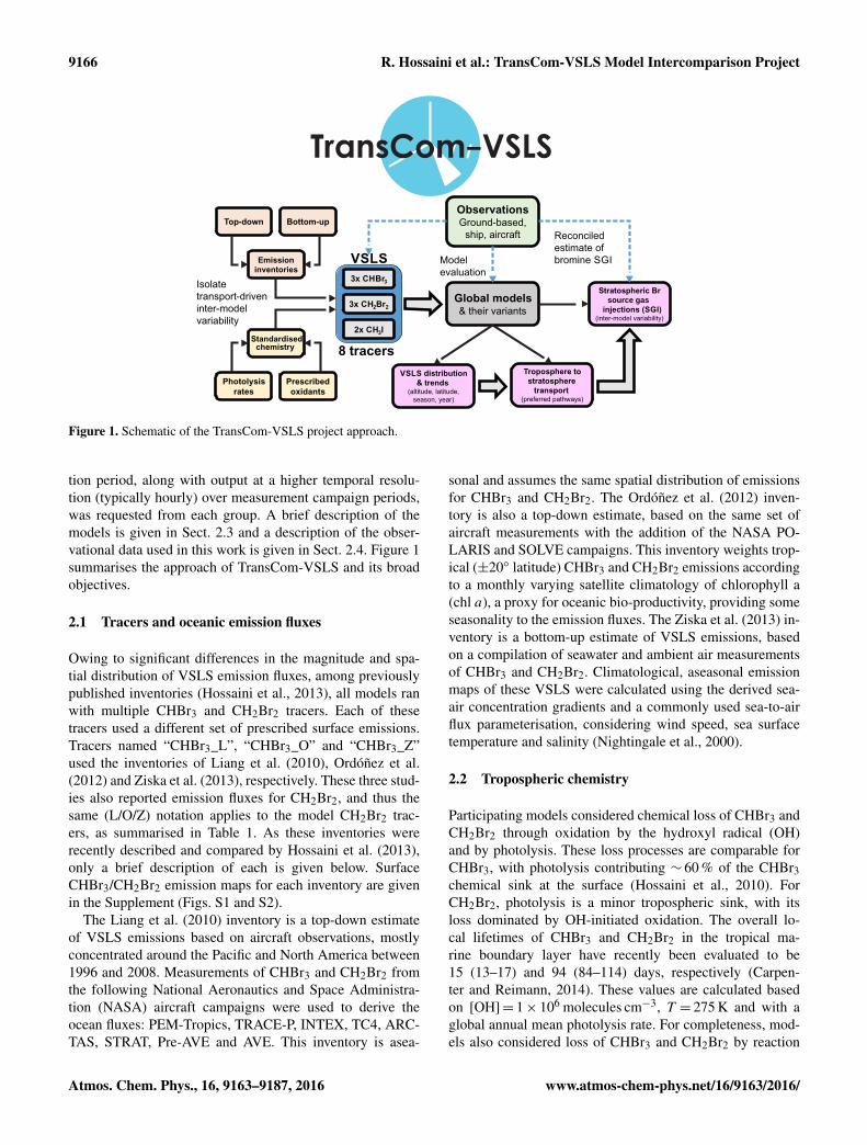
tion period, along with output at a higher temporal resolu-tion (typically hourly) over measurement campaign periods,was requested from each group. A brief description of themodels is given in Sect. 2.3 and a description of the obser-vational data used in this work is given in Sect. 2.4. Figure 1summarises the approach of TransCom-VSLS and its broadobjectives.
2.1 Tracers and oceanic emission fluxes
Owing to significant differences in the magnitude and spa-tial distribution of VSLS emission fluxes, among previouslypublished inventories (Hossaini et al., 2013), all models ranwith multiple CHBr3 and CH2Br2 tracers. Each of thesetracers used a different set of prescribed surface emissions.Tracers named “CHBr3_L”, “CHBr3_O” and “CHBr3_Z”used the inventories of Liang et al. (2010), Ordóñez et al.(2012) and Ziska et al. (2013), respectively. These three stud-ies also reported emission fluxes for CH2Br2, and thus thesame (L/O/Z) notation applies to the model CH2Br2 trac-ers, as summarised in Table 1. As these inventories wererecently described and compared by Hossaini et al. (2013),only a brief description of each is given below. SurfaceCHBr3/CH2Br2 emission maps for each inventory are givenin the Supplement (Figs. S1 and S2).
The Liang et al. (2010) inventory is a top-down estimateof VSLS emissions based on aircraft observations, mostlyconcentrated around the Pacific and North America between1996 and 2008. Measurements of CHBr3 and CH2Br2 fromthe following National Aeronautics and Space Administra-tion (NASA) aircraft campaigns were used to derive theocean fluxes: PEM-Tropics, TRACE-P, INTEX, TC4, ARC-TAS, STRAT, Pre-AVE and AVE. This inventory is asea-
sonal and assumes the same spatial distribution of emissionsfor CHBr3 and CH2Br2. The Ordóñez et al. (2012) inven-tory is also a top-down estimate, based on the same set ofaircraft measurements with the addition of the NASA PO-LARIS and SOLVE campaigns. This inventory weights trop-ical (±20◦ latitude) CHBr3 and CH2Br2 emissions accordingto a monthly varying satellite climatology of chlorophyll a(chl a), a proxy for oceanic bio-productivity, providing someseasonality to the emission fluxes. The Ziska et al. (2013) in-ventory is a bottom-up estimate of VSLS emissions, basedon a compilation of seawater and ambient air measurementsof CHBr3 and CH2Br2. Climatological, aseasonal emissionmaps of these VSLS were calculated using the derived sea-air concentration gradients and a commonly used sea-to-airflux parameterisation, considering wind speed, sea surfacetemperature and salinity (Nightingale et al., 2000).
2.2 Tropospheric chemistry
Participating models considered chemical loss of CHBr3 andCH2Br2 through oxidation by the hydroxyl radical (OH)and by photolysis. These loss processes are comparable forCHBr3, with photolysis contributing ∼ 60 % of the CHBr3chemical sink at the surface (Hossaini et al., 2010). ForCH2Br2, photolysis is a minor tropospheric sink, with itsloss dominated by OH-initiated oxidation. The overall lo-cal lifetimes of CHBr3 and CH2Br2 in the tropical ma-rine boundary layer have recently been evaluated to be15 (13–17) and 94 (84–114) days, respectively (Carpen-ter and Reimann, 2014). These values are calculated basedon [OH]= 1× 10⁶ molecules cm−3, T = 275 K and with aglobal annual mean photolysis rate. For completeness, mod-els also considered loss of CHBr3 and CH2Br2 by reaction
Atmos. Chem. Phys., 16, 9163–9187, 2016 www.atmos-chem-phys.net/16/9163/2016/
R. Hossaini et al.: TransCom-VSLS Model Intercomparison Project 9167
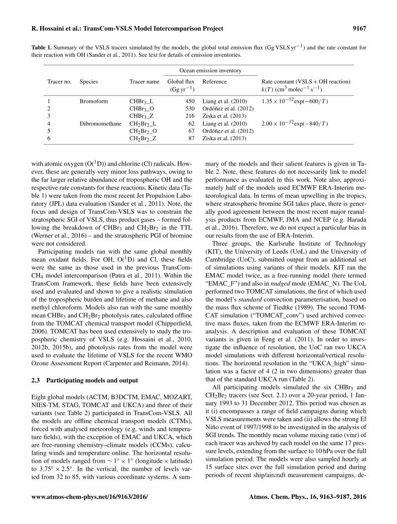
Table 1. Summary of the VSLS tracers simulated by the models, the global total emission flux (Gg VSLS yr−1) and the rate constant fortheir reaction with OH (Sander et al., 2011). See text for details of emission inventories.
Ocean emission inventory
Tracer no. Species Tracer name Global flux Reference Rate constant (VSLS+OH reaction)(Gg yr−1) k(T ) (cm3 molec−1 s−1)
1 Bromoform CHBr3_L 450 Liang et al. (2010) 1.35× 10⁻¹²exp(−600/T )2 CHBr3_O 530 Ordóñez et al. (2012)3 CHBr3_Z 216 Ziska et al. (2013)4 Dibromomethane CH2Br2_L 62 Liang et al. (2010) 2.00× 10⁻¹²exp(−840/T )5 CH2Br2_O 67 Ordóñez et al. (2012)6 CH2Br2_Z 87 Ziska et al. (2013)
with atomic oxygen (O(1D)) and chlorine (Cl) radicals. How-ever, these are generally very minor loss pathways, owing tothe far larger relative abundance of tropospheric OH and therespective rate constants for these reactions. Kinetic data (Ta-ble 1) were taken from the most recent Jet Propulsion Labo-ratory (JPL) data evaluation (Sander et al., 2011). Note, thefocus and design of TransCom-VSLS was to constrain thestratospheric SGI of VSLS, thus product gases – formed fol-lowing the breakdown of CHBr3 and CH2Br2 in the TTL(Werner et al., 2016) – and the stratospheric PGI of brominewere not considered.
Participating models ran with the same global monthlymean oxidant fields. For OH, O(1D) and Cl, these fieldswere the same as those used in the previous TransCom-CH4 model intercomparison (Patra et al., 2011). Within theTransCom framework, these fields have been extensivelyused and evaluated and shown to give a realistic simulationof the tropospheric burden and lifetime of methane and alsomethyl chloroform. Models also ran with the same monthlymean CHBr3 and CH2Br2 photolysis rates, calculated offlinefrom the TOMCAT chemical transport model (Chipperfield,2006). TOMCAT has been used extensively to study the tro-pospheric chemistry of VSLS (e.g. Hossaini et al., 2010,2012b, 2015b), and photolysis rates from the model wereused to evaluate the lifetime of VSLS for the recent WMOOzone Assessment Report (Carpenter and Reimann, 2014).
2.3 Participating models and output
Eight global models (ACTM, B3DCTM, EMAC, MOZART,NIES-TM, STAG, TOMCAT and UKCA) and three of theirvariants (see Table 2) participated in TransCom-VSLS. Allthe models are offline chemical transport models (CTMs),forced with analysed meteorology (e.g. winds and tempera-ture fields), with the exception of EMAC and UKCA, whichare free-running chemistry–climate models (CCMs), calcu-lating winds and temperature online. The horizontal resolu-tion of models ranged from ∼ 1◦× 1◦ (longitude× latitude)to 3.75◦× 2.5◦. In the vertical, the number of levels var-ied from 32 to 85, with various coordinate systems. A sum-
mary of the models and their salient features is given in Ta-ble 2. Note, these features do not necessarily link to modelperformance as evaluated in this work. Note also, approxi-mately half of the models used ECMWF ERA-Interim me-teorological data. In terms of mean upwelling in the tropics,where stratospheric bromine SGI takes place, there is gener-ally good agreement between the most recent major reanal-ysis products from ECMWF, JMA and NCEP (e.g. Haradaet al., 2016). Therefore, we do not expect a particular bias inour results from the use of ERA-Interim.
Three groups, the Karlsruhe Institute of Technology(KIT), the University of Leeds (UoL) and the University ofCambridge (UoC), submitted output from an additional setof simulations using variants of their models. KIT ran theEMAC model twice, as a free-running model (here termed“EMAC_F”) and also in nudged mode (EMAC_N). The UoLperformed two TOMCAT simulations, the first of which usedthe model’s standard convection parameterisation, based onthe mass flux scheme of Tiedtke (1989). The second TOM-CAT simulation (“TOMCAT_conv”) used archived convec-tive mass fluxes, taken from the ECMWF ERA-Interim re-analysis. A description and evaluation of these TOMCATvariants is given in Feng et al. (2011). In order to inves-tigate the influence of resolution, the UoC ran two UKCAmodel simulations with different horizontal/vertical resolu-tions. The horizontal resolution in the “UKCA_high” simu-lation was a factor of 4 (2 in two dimensions) greater thanthat of the standard UKCA run (Table 2).
All participating models simulated the six CHBr3 andCH2Br2 tracers (see Sect. 2.1) over a 20-year period, 1 Jan-uary 1993 to 31 December 2012. This period was chosen asit (i) encompasses a range of field campaigns during whichVSLS measurements were taken and (ii) allows the strong ElNiño event of 1997/1998 to be investigated in the analysis ofSGI trends. The monthly mean volume mixing ratio (vmr) ofeach tracer was archived by each model on the same 17 pres-sure levels, extending from the surface to 10 hPa over the fullsimulation period. The models were also sampled hourly at15 surface sites over the full simulation period and duringperiods of recent ship/aircraft measurement campaigns, de-
www.atmos-chem-phys.net/16/9163/2016/ Atmos. Chem. Phys., 16, 9163–9187, 2016
9168 R. Hossaini et al.: TransCom-VSLS Model Intercomparison Project
Table2.O
verviewofTransC
om-V
SLS
models
andm
odelvariants.
No.
Model a
Institution bR
esolutionM
eteorology eB
oundarylayerm
ixingC
onvectionR
eference
Horizontal c
Vertical d
1A
CT
MJA
MST
EC
2.8◦×
2.8◦
67σ
JRA
-25M
ellorandY
amada
(1974)A
rakawa
andShubert(1974)
Patraetal.(2009)
2B
3DC
TM
UoB
3.75◦×
2.5◦
40σ
-θE
CM
WF
ER
A-Interim
Simple g
ER
A-Interim
,archived hA
schmann
etal.(2014)3
EM
AC
f(_free)K
IT2.8◦×
2.8◦
39σ
-pO
nline,free-runningJöckeletal.(2006)
Tiedtke(1989) i
Jöckeletal.(2006,2010)4
EM
AC(_nudged)
KIT
2.8◦×
2.8◦
39σ
-pN
udgedto
ER
A-Interim
Jöckeletal.(2006)Tiedtke
(1989) iJöckeletal.(2006,2010)
5M
OZ
AR
TE
MU
2.5◦×
1.9◦
56σ
-pM
ER
RA
Holtslag
andB
oville(1993)
jE
mm
onsetal.(2010)
6N
IES-T
MN
IES
2.5◦×
2.5◦
32σ
-θJC
DA
S(JR
A-25)
Belikov
etal.(2013)Tiedtke
(1989)B
elikovetal.(2011,2013)
7STA
GA
IST1.125
◦×
1.125◦
60σ
-pE
CM
WF
ER
A-Interim
Taguchietal.(2013)Taguchietal.(2013)
Taguchi(1996)8
TOM
CA
TU
oL2.8◦×
2.8◦
60σ
-pE
CM
WF
ER
A-Interim
Holtslag
andB
oville(1993)
Tiedtke(1989)
Chipperfield
(2009)9
TOM
CAT
(_conv)U
oL2.8◦×
2.8◦
60σ
-pE
CM
WF
ER
A-Interim
Holtslag
andB
oville(1993)
ER
A-Interim
,archived hC
hipperfield(2009)
10U
KC
A(_low
)U
oC/N
CA
S3.75◦×
2.5◦
60σ
-zO
nline,free-runningL
ocketal.(2000)
Gregory
andR
owntree
(1990)M
orgensternetal.(2009)
11U
KC
A(_high)
UoC
/NC
AS
1.875◦×
1.25◦
85σ
-zO
nline,free-runningL
ocketal.(2000)
Gregory
andR
owntree
(1990)M
orgensternetal.(2009)
aA
llmodels
areoffline
CT
Ms
exceptboldentries
which
areC
CM
s.Modelvariants
areshow
nin
italics.CC
Ms
ranusing
prescribedsea
surfacetem
peraturesfrom
observations. bJA
MST
EC
:JapanA
gencyforM
arine-Earth
Scienceand
Technology,Japan;U
oB:U
niversityofB
remen,G
ermany;K
IT:Karlsruhe
InstituteofTechnology,G
ermany;E
MU
:Em
oryU
niversity,USA
;NIE
S:NationalInstitute
forEnvironm
entalStudies,Japan;AIST:N
ationalInstituteofA
dvancedIndustrialScience
andTechnology,
Japan;UoL
:University
ofLeeds,U
K;U
oC:U
niversityofC
ambridge,U
K;N
CA
S:NationalC
entreforA
tmospheric
Science,UK
. cL
ongitude×
latitude. dσ
:terrain-following
sigma
levels(pressure
dividedby
surfacepressure);
σ-p
:hybridsigm
a-pressure;σ
-θ:hybridsigm
a-potentialtemperature;
σ-z:hybrid
sigma-height. e
ME
RR
A:M
odern-eraR
etrospectiveA
nalysisforR
esearchand
Applications;JC
DA
S:JapanM
eteorologicalAgency
Clim
ateD
ataA
ssimilation
System;JR
A-25:
Japanese25-yearR
eAnalysis;E
CM
WF:E
uropeanC
entreforM
edium-range
WeatherForecasts. f
EC
HA
M/M
ESSy
Atm
osphericC
hemistry
(EM
AC
)model(R
oeckneretal.,2006).EC
HA
M5
version5.3.02.M
ESSy
version2.42. g
Simple
averagingof
tracermixing
ratiobelow
ER
A-Interim
boundarylayerheight. h
Read-in
convectivem
assfluxes
fromE
CM
WF
ER
A-Interim
.SeeA
schmann
etal.(2011)forB3D
CT
Mim
plementation
andFeng
etal.(2011)forTOM
CA
Tim
plementation. iW
ithm
odificationsfrom
Nordeng
(1994). jShallow&
mid-levelconvection
(Hack,1994);deep
convection(Z
hangand
McFarlane,1995).
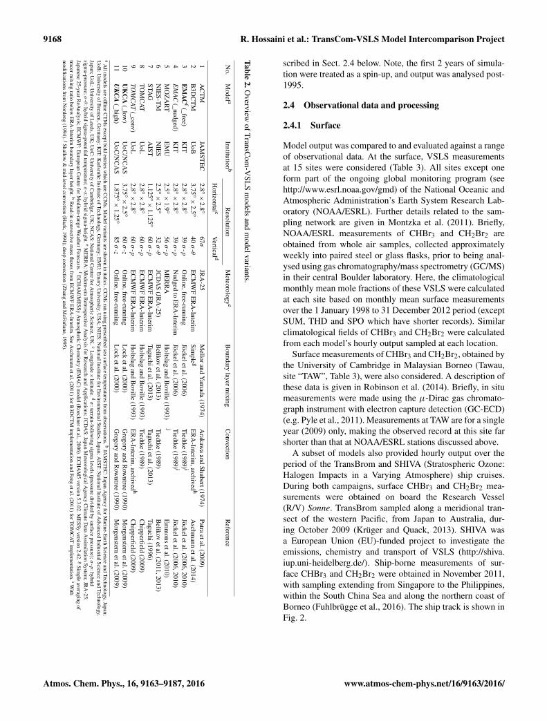
scribed in Sect. 2.4 below. Note, the first 2 years of simula-tion were treated as a spin-up, and output was analysed post-1995.
2.4 Observational data and processing
2.4.1 Surface
Model output was compared to and evaluated against a rangeof observational data. At the surface, VSLS measurementsat 15 sites were considered (Table 3). All sites except oneform part of the ongoing global monitoring program (seehttp://www.esrl.noaa.gov/gmd) of the National Oceanic andAtmospheric Administration’s Earth System Research Lab-oratory (NOAA/ESRL). Further details related to the sam-pling network are given in Montzka et al. (2011). Briefly,NOAA/ESRL measurements of CHBr3 and CH2Br2 areobtained from whole air samples, collected approximatelyweekly into paired steel or glass flasks, prior to being anal-ysed using gas chromatography/mass spectrometry (GC/MS)in their central Boulder laboratory. Here, the climatologicalmonthly mean mole fractions of these VSLS were calculatedat each site based on monthly mean surface measurementsover the 1 January 1998 to 31 December 2012 period (exceptSUM, THD and SPO which have shorter records). Similarclimatological fields of CHBr3 and CH2Br2 were calculatedfrom each model’s hourly output sampled at each location.
Surface measurements of CHBr3 and CH2Br2, obtained bythe University of Cambridge in Malaysian Borneo (Tawau,site “TAW”, Table 3), were also considered. A description ofthese data is given in Robinson et al. (2014). Briefly, in situmeasurements were made using the µ-Dirac gas chromato-graph instrument with electron capture detection (GC-ECD)(e.g. Pyle et al., 2011). Measurements at TAW are for a singleyear (2009) only, making the observed record at this site farshorter than that at NOAA/ESRL stations discussed above.
A subset of models also provided hourly output over theperiod of the TransBrom and SHIVA (Stratospheric Ozone:Halogen Impacts in a Varying Atmosphere) ship cruises.During both campaigns, surface CHBr3 and CH2Br2 mea-surements were obtained on board the Research Vessel(R/V) Sonne. TransBrom sampled along a meridional tran-sect of the western Pacific, from Japan to Australia, dur-ing October 2009 (Krüger and Quack, 2013). SHIVA wasa European Union (EU)-funded project to investigate theemissions, chemistry and transport of VSLS (http://shiva.iup.uni-heidelberg.de/). Ship-borne measurements of sur-face CHBr3 and CH2Br2 were obtained in November 2011,with sampling extending from Singapore to the Philippines,within the South China Sea and along the northern coast ofBorneo (Fuhlbrügge et al., 2016). The ship track is shown inFig. 2.
Atmos. Chem. Phys., 16, 9163–9187, 2016 www.atmos-chem-phys.net/16/9163/2016/

R. Hossaini et al.: TransCom-VSLS Model Intercomparison Project 9169
-9090 180
30
90 180 -90
90 180 -90
-30
30
-30
30
Surface ATTREX 13 ATTERX 14 CAST HIPPO-1 HIPPO-2 HIPPO-3
HIPPO-4 HIPPO-5 Pre-Ave CR-AVE SHIVA (ship) TransBrom (ship)
0
Figure 2. Summary of ground-based and campaign data used inTransCom-VSLS. See main text for details.
2.4.2 Aircraft
Observations of CHBr3 and CH2Br2 from a range of aircraftcampaigns were also used (Fig. 2). As (i) the troposphere-to-stratosphere transport of air (and VSLS) primarily occursin the tropics, and (ii) because VSLS emitted in the ex-tratropics have a negligible impact on stratospheric ozone(Tegtmeier et al., 2015), TransCom-VSLS focused on aircraftmeasurements obtained in the latitude range 30◦ N to 30◦ S.Hourly model output was interpolated to the relevant air-craft sampling location, allowing for point-by-point model–measurement comparisons. A brief description of the aircraftcampaigns follows.
The HIAPER Pole-to-Pole Observations (HIPPO) project(http://www.eol.ucar.edu/projects/hippo) comprised a seriesof aircraft campaigns between 2009 and 2011 (Wofsyet al., 2011), supported by the National Science Foun-dation (NSF). Five campaigns were conducted: HIPPO-1 (January 2009), HIPPO-2 (November 2009), HIPPO-3(March/April 2010), HIPPO-4 (June 2011) and HIPPO-5(August/September 2011). Sampling spanned a range of lat-itudes, from near the North Pole to coastal Antarctica, onboard the NSF Gulfstream V aircraft, and from the surfaceto ∼ 14 km over the Pacific Basin. Whole air samples, col-lected in stainless steel and glass flasks, were analysed bytwo different laboratories using GC/MS (NOAA/ESRL andthe University of Miami). HIPPO results from both laborato-ries are provided on a scale consistent with NOAA/ESRL.
The SHIVA aircraft campaign, based in Miri (MalaysianBorneo), was conducted during November–December 2011.Measurements of CHBr3 and CH2Br2 were obtained dur-ing 14 flights of the DLR Falcon aircraft, with samplingover much of the northern coast of Borneo, within the SouthChina and Sulu seas, up to an altitude of∼ 12 km (Sala et al.,2014; Fuhlbrügge et al., 2016). VSLS measurements wereobtained by two groups, the University of Frankfurt (UoF)and the University of East Anglia (UEA). UoF measure-ments were made using an in situ GC/MS system (Sala et al.,
2014), while UEA analysed collected whole air samples, us-ing GC/MS.
CAST (Coordinated Airborne Studies in the Tropics) isan ongoing research project funded by the UK Natural En-vironment Research Council (NERC) and is a collaborativeinitiative with the NASA ATTREX programme (see below).The CAST aircraft campaign, based in Guam, was conductedin January–February 2014 with VSLS measurements madeby the University of York on board the FAAM (Facility forAirborne Atmospheric Measurements) BAe-146 aircraft, upto an altitude of ∼ 8 km. These observations were made byGC/MS collected from whole air samples as described in An-drews et al. (2016).
Observations of CHBr3 and CH2Br2 within the TTL andlower stratosphere (up to ∼ 20 km) were obtained duringthe NASA (i) Pre-Aura Validation Experiment (Pre-AVE),(ii) Costa Rica Aura Validation Experiment (CR-AVE) and(iii) Airborne Tropical TRopopause EXperiment (ATTREX)missions. The Pre-AVE mission was conducted in 2004(January–February), with measurements obtained over theequatorial eastern Pacific during eight flights of the high-altitude WB-57 aircraft. The CR-AVE mission took placein 2006 (January–February) and sampled a similar regionaround Costa Rica (Fig. 2), also with the WB-57 aircraft (15flights). The ATTREX mission consists of an ongoing se-ries of aircraft campaigns using the unmanned Global Hawkaircraft. Here, CHBr3 and CH2Br2 measurements from 10flights of the Global Hawk, over two ATTREX campaigns,were used. The first campaign (February–March 2013) sam-pled large stretches of the north-east and central PacificOcean, while the second campaign (January–March 2014)sampled predominantly the western Pacific, around Guam.During Pre-AVE, CR-AVE and ATTREX, VSLS measure-ments were obtained by the University of Miami followingGC/MS analysis of collected whole air samples.
3 Results and discussion
3.1 Model–observation comparisons: surface
In this section, we evaluate the models in terms of (i) theirability to capture the observed seasonal cycle of CHBr3 andCH2Br2 at the surface and (ii) the absolute agreement to theobservations. We focus on investigating the relative perfor-mance of each of the tested emission inventories, within agiven model, and the performance of the inventories acrossthe ensemble.
3.1.1 Seasonality
We first consider the seasonal cycle of CHBr3 and CH2Br2 atthe locations given in Table 3. Figure 3 compares observedand simulated (CHBr3_L tracer) monthly mean anomalies,calculated by subtracting the climatological monthly meanCHBr3 surface mole fraction from the climatological annual
www.atmos-chem-phys.net/16/9163/2016/ Atmos. Chem. Phys., 16, 9163–9187, 2016

9170 R. Hossaini et al.: TransCom-VSLS Model Intercomparison Project
ALT
0 2 4 6 8 10 12
-1.50
-0.75
0.00
0.75
1.50
Anom
aly
[ppt]
SUM
0 2 4 6 8 10 12
-1.50
-0.75
0.00
0.75
1.50BRW
0 2 4 6 8 10 12
-2
-1
0
1
2MHD
0 2 4 6 8 10 12
-2
-1
0
1
2
LEF
0 2 4 6 8 10 12
-1.0
-0.5
0.0
0.5
1.0
Anom
aly
[ppt]
HFM
0 2 4 6 8 10 12
-1.0
-0.5
0.0
0.5
1.0THD
0 2 4 6 8 10 12
-1.0
-0.5
0.0
0.5
1.0NWR
0 2 4 6 8 10 12
-1.0
-0.5
0.0
0.5
1.0
KUM
0 2 4 6 8 10 12
-0.50
-0.25
0.00
0.25
0.50
Anom
aly
[ppt]
MLO
0 2 4 6 8 10 12
-0.50
-0.25
0.00
0.25
0.50TAW
0 2 4 6 8 10 12
-1.50
-0.75
0.00
0.75
1.50SMO
0 2 4 6 8 10 12Month
-0.50
-0.25
0.00
0.25
0.50
CGO
0 2 4 6 8 10 12Month
-1.0
-0.5
0.0
0.5
1.0
Anom
aly
[ppt]
PSA
0 2 4 6 8 10 12Month
-1.0
-0.5
0.0
0.5
1.0SPO
0 2 4 6 8 10 12Month
-1.0
-0.5
0.0
0.5
1.0ACTM B3DCTM
EMAC_F EMAC_N
MOZART NIES-TM
STAG TOMCAT
TOMCAT_C UKCA_LO
UKCA_HI Obs.
Figure 3. Comparison of the observed and simulated seasonal cycle of surface CHBr3 at ground-based measurement sites (see Table 3). Theseasonal cycle is shown here as climatological (1998–2011) monthly mean anomalies, calculated by subtracting the climatological monthlymean CHBr3 mole fraction (ppt) from the climatological annual mean, in both the observed (black points) and model (coloured lines; seelegend) data sets. The location of the surface sites is summarised in Table 3. Model output based on CHBr3_L tracer (i.e. using aseasonalemissions inventory of Liang et al., 2010). Horizontal bars denote ±1σ .
Table 3. Summary and location of ground-based surface VSLSmeasurements used in TransCom-VSLS, arranged from north tosouth. All sites are part of the NOAA/ESRL global monitoring net-work, with the exception of TAW, at which measurements were ob-tained by the University of Cambridge (see main text). ∗ StationsSUM, MLO and SPO are elevated at ∼ 3210, 3397 and 2810 m, re-spectively.
Station Site name Latitude Longitude
ALT Alert, NW Territories, Canada 82.5◦ N 62.3◦WSUM∗ Summit, Greenland 72.6◦ N 38.4◦WBRW Pt. Barrow, Alaska, USA 71.3◦ N 156.6◦WMHD Mace Head, Ireland 53.0◦ N 10.0◦WLEF Wisconsin, USA 45.6◦ N 90.2◦WHFM Harvard Forest, USA 42.5◦ N 72.2◦WTHD Trinidad Head, USA 41.0◦ N 124.0◦WNWR Niwot Ridge, Colorado, USA 40.1◦ N 105.6◦WKUM Cape Kumukahi, Hawaii, USA 19.5◦ N 154.8◦WMLO∗ Mauna Loa, Hawaii, USA 19.5◦ N 155.6◦WTAW Tawau, Sabah, Malaysian Borneo 4.2◦ N 117.9◦ ESMO Cape Matatula, American Samoa 14.3◦ S 170.6◦WCGO Cape Grim, Tasmania, Australia 40.7◦ S 144.8◦ EPSA Palmer Station, Antarctica 64.6◦ S 64.0◦WSPO∗ South Pole 90.0◦ S –
mean (to focus on the seasonal variability). Based on pho-tochemistry alone, in the Northern Hemisphere (NH), onewould expect a CHBr3 winter (December–February) maxi-mum owing to a reduced chemical sink (e.g. slower photol-ysis rates and lower [OH]) and thereby a relatively longerCHBr3 lifetime. This seasonality, apparent at most NH sitesshown in Fig. 3, is particularly pronounced at high latitudes(> 60◦ N, e.g. ALT, BRW and SUM), where the amplitude ofthe observed seasonal cycle is greatest. A number of featuresare apparent from these comparisons. First, in general, mostmodels reproduce the observed phase of the CHBr3 seasonalcycle well, even with emissions that do not vary seasonally,suggesting that seasonal variations in the CHBr3 chemicalsink are generally well represented. For example, model–measurement correlation coefficients (r), summarised in Ta-ble 4, are > 0.7 for at least 80 % of the models at 7 of 11NH sites. Second, at some sites, notably MHD, THD, CGOand PSA, the observed seasonal cycle of CHBr3 is not cap-tured well by virtually all of the models (see discussion be-low). Third, at most sites the amplitude of the seasonal cy-cle is generally consistent across the models (within a fewpercent, excluding clear outliers). The cause of outliers at agiven site is likely in part related to the model sampling er-ror, including distance of a model grid from the measurement
Atmos. Chem. Phys., 16, 9163–9187, 2016 www.atmos-chem-phys.net/16/9163/2016/
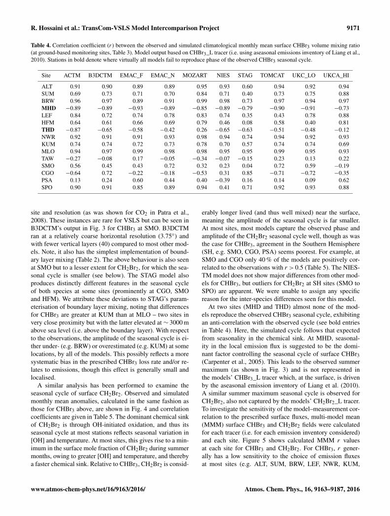
R. Hossaini et al.: TransCom-VSLS Model Intercomparison Project 9171
Table 4. Correlation coefficient (r) between the observed and simulated climatological monthly mean surface CHBr3 volume mixing ratio(at ground-based monitoring sites, Table 3). Model output based on CHBr3_L tracer (i.e. using aseasonal emissions inventory of Liang et al.,2010). Stations in bold denote where virtually all models fail to reproduce phase of the observed CHBr3 seasonal cycle.
Site ACTM B3DCTM EMAC_F EMAC_N MOZART NIES STAG TOMCAT UKC_LO UKCA_HI
ALT 0.91 0.90 0.89 0.89 0.95 0.93 0.60 0.94 0.92 0.94SUM 0.69 0.73 0.71 0.70 0.84 0.71 0.40 0.73 0.75 0.88BRW 0.96 0.97 0.89 0.91 0.99 0.98 0.73 0.97 0.94 0.97MHD −0.89 −0.89 −0.93 −0.89 −0.85 −0.89 −0.79 −0.90 −0.91 −0.73LEF 0.84 0.72 0.74 0.78 0.83 0.74 0.35 0.43 0.78 0.88HFM 0.64 0.61 0.66 0.69 0.79 0.46 0.08 0.58 0.40 0.81THD −0.87 −0.65 −0.58 −0.42 0.26 −0.65 −0.63 −0.51 −0.48 −0.12NWR 0.92 0.91 0.91 0.93 0.98 0.94 0.74 0.94 0.92 0.93KUM 0.74 0.74 0.72 0.73 0.78 0.70 0.57 0.74 0.74 0.69MLO 0.94 0.97 0.99 0.98 0.98 0.95 0.95 0.99 0.95 0.93TAW −0.27 −0.08 0.17 −0.05 −0.34 −0.07 −0.15 0.23 0.13 0.22SMO 0.56 0.45 0.43 0.72 0.32 0.23 0.04 0.72 0.59 −0.19CGO −0.64 0.72 −0.22 −0.18 −0.53 0.31 0.85 −0.71 −0.72 −0.35PSA 0.13 0.24 0.60 0.44 0.40 −0.39 0.16 0.14 0.09 0.62SPO 0.90 0.91 0.85 0.89 0.94 0.41 0.71 0.92 0.93 0.88
site and resolution (as was shown for CO2 in Patra et al.,2008). These instances are rare for VSLS but can be seen inB3DCTM’s output in Fig. 3 for CHBr3 at SMO. B3DCTMran at a relatively coarse horizontal resolution (3.75◦) andwith fewer vertical layers (40) compared to most other mod-els. Note, it also has the simplest implementation of bound-ary layer mixing (Table 2). The above behaviour is also seenat SMO but to a lesser extent for CH2Br2, for which the sea-sonal cycle is smaller (see below). The STAG model alsoproduces distinctly different features in the seasonal cycleof both species at some sites (prominently at CGO, SMOand HFM). We attribute these deviations to STAG’s param-eterisation of boundary layer mixing, noting that differencesfor CHBr3 are greater at KUM than at MLO – two sites invery close proximity but with the latter elevated at ∼ 3000 mabove sea level (i.e. above the boundary layer). With respectto the observations, the amplitude of the seasonal cycle is ei-ther under- (e.g. BRW) or overestimated (e.g. KUM) at somelocations, by all of the models. This possibly reflects a moresystematic bias in the prescribed CHBr3 loss rate and/or re-lates to emissions, though this effect is generally small andlocalised.
A similar analysis has been performed to examine theseasonal cycle of surface CH2Br2. Observed and simulatedmonthly mean anomalies, calculated in the same fashion asthose for CHBr3 above, are shown in Fig. 4 and correlationcoefficients are given in Table 5. The dominant chemical sinkof CH2Br2 is through OH-initiated oxidation, and thus itsseasonal cycle at most stations reflects seasonal variation in[OH] and temperature. At most sites, this gives rise to a min-imum in the surface mole fraction of CH2Br2 during summermonths, owing to greater [OH] and temperature, and therebya faster chemical sink. Relative to CHBr3, CH2Br2 is consid-
erably longer lived (and thus well mixed) near the surface,meaning the amplitude of the seasonal cycle is far smaller.At most sites, most models capture the observed phase andamplitude of the CH2Br2 seasonal cycle well, though as wasthe case for CHBr3, agreement in the Southern Hemisphere(SH, e.g. SMO, CGO, PSA) seems poorest. For example, atSMO and CGO only 40 % of the models are positively cor-related to the observations with r > 0.5 (Table 5). The NIES-TM model does not show major differences from other mod-els for CHBr3, but outliers for CH2Br2 at SH sites (SMO toSPO) are apparent. We were unable to assign any specificreason for the inter-species differences seen for this model.
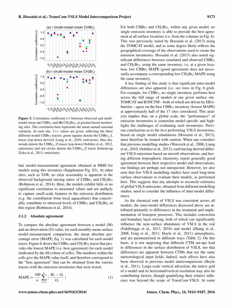
At two sites (MHD and THD) almost none of the mod-els reproduce the observed CHBr3 seasonal cycle, exhibitingan anti-correlation with the observed cycle (see bold entriesin Table 4). Here, the simulated cycle follows that expectedfrom seasonality in the chemical sink. At MHD, seasonal-ity in the local emission flux is suggested to be the domi-nant factor controlling the seasonal cycle of surface CHBr3(Carpenter et al., 2005). This leads to the observed summermaximum (as shown in Fig. 3) and is not represented inthe models’ CHBr3_L tracer which, at the surface, is drivenby the aseasonal emission inventory of Liang et al. (2010).A similar summer maximum seasonal cycle is observed forCH2Br2, also not captured by the models’ CH2Br2_L tracer.To investigate the sensitivity of the model–measurement cor-relation to the prescribed surface fluxes, multi-model mean(MMM) surface CHBr3 and CH2Br2 fields were calculatedfor each tracer (i.e. for each emission inventory considered)and each site. Figure 5 shows calculated MMM r valuesat each site for CHBr3 and CH2Br2. For CHBr3, r gener-ally has a low sensitivity to the choice of emission fluxesat most sites (e.g. ALT, SUM, BRW, LEF, NWR, KUM,
www.atmos-chem-phys.net/16/9163/2016/ Atmos. Chem. Phys., 16, 9163–9187, 2016

9172 R. Hossaini et al.: TransCom-VSLS Model Intercomparison Project
ALT
0 2 4 6 8 10 12
-0.30
-0.15
0.00
0.15
0.30
Anom
aly
[ppt]
SUM
0 2 4 6 8 10 12
-0.30
-0.15
0.00
0.15
0.30BRW
0 2 4 6 8 10 12
-0.30
-0.15
0.00
0.15
0.30MHD
0 2 4 6 8 10 12
-0.30
-0.15
0.00
0.15
0.30
LEF
0 2 4 6 8 10 12
-0.30
-0.15
0.00
0.15
0.30
Anom
aly
[ppt]
HFM
0 2 4 6 8 10 12
-0.30
-0.15
0.00
0.15
0.30THD
0 2 4 6 8 10 12
-0.30
-0.15
0.00
0.15
0.30NWR
0 2 4 6 8 10 12
-0.30
-0.15
0.00
0.15
0.30
KUM
0 2 4 6 8 10 12
-0.30
-0.15
0.00
0.15
0.30
Anom
aly
[ppt]
MLO
0 2 4 6 8 10 12
-0.30
-0.15
0.00
0.15
0.30TAW
0 2 4 6 8 10 12
-0.30
-0.15
0.00
0.15
0.30SMO
0 2 4 6 8 10 12Month
-0.30
-0.15
0.00
0.15
0.30
CGO
0 2 4 6 8 10 12Month
-0.30
-0.15
0.00
0.15
0.30
Anom
aly
[ppt]
PSA
0 2 4 6 8 10 12Month
-0.30
-0.15
0.00
0.15
0.30SPO
0 2 4 6 8 10 12Month
-0.30
-0.15
0.00
0.15
0.30ACTM B3DCTM
EMAC_F EMAC_N
MOZART NIES-TM
STAG TOMCAT
TOMCAT_C UKCA_LO
UKCA_HI Obs.
Figure 4. As Fig. 3 but for CH2Br2.
Table 5. As Table 4 but for CH2Br2.
Site ACTM B3DCTM EMAC_F EMAC_N MOZART NIES STAG TOMCAT UKCA_LO UKCA_HI
ALT 0.90 0.97 0.79 0.82 0.96 0.98 0.77 0.94 0.85 0.96SUM 0.71 0.93 0.75 0.76 0.92 0.91 0.87 0.77 0.79 0.96BRW 0.87 0.92 0.82 0.85 0.93 0.91 0.90 0.88 0.93 0.93MHD −0.65 −0.73 −0.72 −0.69 −0.76 −0.75 −0.64 −0.72 −0.71 −0.76LEF 0.87 0.73 0.84 0.84 0.94 0.94 0.47 0.62 0.88 0.96HFM 0.82 0.79 0.83 0.84 0.95 0.90 −0.02 0.75 0.72 0.92THD 0.54 0.80 0.73 0.79 0.78 0.84 0.04 0.69 0.66 0.75NWR 0.90 0.88 0.91 0.89 0.99 0.97 0.86 0.91 0.92 0.97KUM 0.90 0.89 0.90 0.91 0.99 0.91 0.74 0.90 0.92 0.98MLO 0.90 0.89 0.94 0.91 0.96 0.90 0.30 0.91 0.93 0.97TAW −0.83 −0.80 −0.78 −0.75 −0.39 −0.47 −0.12 0.15 0.20 −0.16SMO −0.08 0.67 −0.14 0.59 0.38 −0.12 0.34 0.97 0.74 0.00CGO 0.59 −0.43 0.45 0.30 0.64 −0.06 −0.42 0.80 0.80 0.41PSA 0.17 0.71 0.52 0.68 0.75 0.08 0.62 0.72 0.65 0.68SPO 0.88 0.91 0.82 0.86 0.95 −0.04 0.97 0.90 0.94 0.88
MLO, SPO), though notably at MHD, use of the Ziska et al.(2013) inventory (which is aseasonal) reverses the sign of rto give a strong positive correlation (MMM r > 0.70) againstthe observations. Individual model r values for MHD aregiven in Table S1 of the Supplement. With the exceptionof TOMCAT, TOMCAT_CONV and UKCA_HI, the remain-ing seven models each reproduce the MHD CHBr3 seasonal-ity well (with r > 0.65). That good agreement obtained withthe Ziska aseasonal inventory, compared to the other asea-
sonal inventories considered, highlights the importance ofthe CHBr3 emission distribution, with respect to transportprocesses, serving this location. We suggest that the sum-mertime transport of air that has experienced relatively largeCHBr3 emissions north/north-west of MHD is the cause ofthe apparent seasonal cycle seen in most models using theZiska inventory (example animations of the seasonal evolu-tion of surface CHBr3 are given in the Supplementary In-formation to visualise this). Note also, the far better abso-
Atmos. Chem. Phys., 16, 9163–9187, 2016 www.atmos-chem-phys.net/16/9163/2016/
R. Hossaini et al.: TransCom-VSLS Model Intercomparison Project 9173
(a) r (multi-model mean CHBr3)
-1.0
-0.5
0.0
0.5
1.0
Co
rre
latio
n c
oe
fficie
nt
(r)
ALT
SUMBRWM
HDLE
FHFM
THDNW
R
KUMM
LOTA
WSM
OCG
OPSASPO
(b) r (multi-model mean CH2Br2)
-1.0
-0.5
0.0
0.5
1.0
Co
rre
latio
n c
oe
fficie
nt
(r)
ALT
SUMBRWM
HDLE
FHFM
THDNW
R
KUMM
LOTA
WSM
OCG
OPSASPO
Figure 5. Correlation coefficient (r) between observed and multi-model mean (a) CHBr3 and (b) CH2Br2, at ground-based monitor-ing sites. The correlation here represents the mean annual seasonalvariation. At each site, 3×r values are given, reflecting the threedifferent model CHBr3 tracers; green squares denote the CHBr3_Ltracer (top-down derived, Liang et al., 2010, emissions), blue dia-monds denote the CHBr3_O tracer (top-down Ordóñez et al., 2012,emissions) and red circles denote the CHBr3_Z tracer (bottom-upZiska et al., 2013, emissions).
lute model–measurement agreement obtained at MHD formodels using this inventory (Supplement Fig. S3). At othersites, such as TAW, no clear seasonality is apparent in theobserved background mixing ratios of CHBr3 and CH2Br2(Robinson et al., 2014). Here, the models exhibit little or nosignificant correlation to measured values and are unlikelyto capture small-scale features in the emission distribution(e.g. the contribution from local aquaculture) that conceiv-ably contribute to observed levels of CHBr3 and CH2Br2 inthis region (Robinson et al., 2014).
3.1.2 Absolute agreement
To compare the absolute agreement between a model (M)and an observation (O) value, for each monthly mean surfacemodel–measurement comparison, the mean absolute per-centage error (MAPE, Eq. 1) was calculated for each modeltracer. Figure 6 shows the CHBr3 and CH2Br2 tracer that pro-vides the lowest MAPE (i.e. best agreement) for each model(indicated by the fill colour of cells). The numbers within thecells give the MAPE value itself, and therefore correspond tothe “best agreement” that can be obtained from the varioustracers with the emission inventories that were tested.
MAPE=100n
n∑t=1|Mt −Ot
Ot| (1)
For both CHBr3 and CH2Br2, within any given model, nosingle emission inventory is able to provide the best agree-ment at all surface locations (i.e. from the columns in Fig. 6).This was previously noted by Hossaini et al. (2013) usingthe TOMCAT model, and to some degree likely reflects thegeographical coverage of the observations used to create theemission inventories. Hossaini et al. (2013) also noted sig-nificant differences between simulated and observed CHBr3and CH2Br2, using the same inventory; i.e. at a given loca-tion, low CHBr3 MAPE (good agreement) does not neces-sarily accompany a corresponding low CH2Br2 MAPE usingthe same inventory.
A key finding of this study is that significant inter-modeldifferences are also apparent (i.e. see rows in Fig. 6 grid).For example, for CHBr3, no single inventory performs bestacross the full range of models at any given surface site.TOMCAT and B3DCTM – both of which are driven by ERA-Interim – agree on the best CHBr3 inventory (lowest MAPE)at approximately half of the 17 sites considered. This anal-ysis implies that, on a global scale, the “performance” ofemission inventories is somewhat model-specific and high-lights the challenges of evaluating such inventories. Previ-ous conclusions as to the best performing VSLS inventories,based on single model simulations (Hossaini et al., 2013),must therefore be treated with caution. When one considersthat previous modelling studies (Warwick et al., 2006; Lianget al., 2010; Ordóñez et al., 2012), each having derived differ-ent VSLS emissions based on aircraft observations, and hav-ing different tropospheric chemistry, report generally goodagreement between their respective model and observations,our findings are perhaps not unexpected. However, we alsonote that few VSLS modelling studies have used long-termsurface observations to evaluate their models, as performedhere. This suggests that any attempts to reconcile estimatesof global VSLS emissions, obtained from different modellingstudies, need to consider the influence of inter-model differ-ences.
As the chemical sink of VSLS was consistent across allmodels, the inter-model differences discussed above are at-tributed primarily to differences in the treatment and imple-mentation of transport processes. This includes convectionand boundary layer mixing, both of which can significantlyinfluence the near-surface abundance of VSLS in the real(Fuhlbrügge et al., 2013, 2016) and model (Zhang et al.,2008; Feng et al., 2011; Hoyle et al., 2011) atmospheres,and are parameterised in different ways (Table 2). On thisbasis, it is not surprising that different CTM set-ups leadto differences in the surface distribution of VSLS, nor thatdifferences are apparent between CTMs that use the samemeteorological input fields. Indeed, such effects have alsobeen observed in previous model intercomparisons (Hoyleet al., 2011). Large-scale vertical advection, the native gridof a model and its horizontal/vertical resolution may also becontributing factors, though quantifying their relative influ-ence was beyond the scope of TransCom-VSLS. At some
www.atmos-chem-phys.net/16/9163/2016/ Atmos. Chem. Phys., 16, 9163–9187, 2016

9174 R. Hossaini et al.: TransCom-VSLS Model Intercomparison Project
Model
SPOPSACGO
*SMO*TAW
*SHIVA
*MLO*KUMNWRTHDHFMLEF
MHDBRWSUMALT
ACTM
B3D
CTM
EM
AC-F
EM
AC-N
MO
ZART
NIE
S-TM
STA
G
TOM
CAT
TOM
CAT_C
UKCA_LO
UKCA_H
I
17
17
34
45
21
***
51
22
17
33
39
32
28
12
21
33
25
19
20
17
55
21
42
51
28
16
52
30
19
23
32
14
35
39
35
37
27
16
18
29
59
32
14
30
61
23
25
15
30
26
15
34
34
31
31
16
29
49
36
14
29
61
24
24
15
29
19
16
17
20
18
17
18
***
***
21
13
21
18
29
26
13
27
28
18
40
23
44
49
16
***
***
18
15
28
29
18
20
28
24
20
29
145
69
11
283
63
***
***
174
112
192
95
175
183
21
90
200
133
16
28
20
4
42
41
53
33
17
30
69
26
24
20
35
29
13
28
27
20
7
24
37
47
31
12
14
55
26
28
20
35
32
18
16
31
31
9
21
***
***
36
16
40
27
60
21
22
18
22
18
17
15
37
17
15
***
***
46
16
41
22
14
19
17
23
19
13
(a) CHBr3 (b) CH2Br2
Model
SPOPSACGO
*SMO*TAW
*SHIVA*TransBrom
*MLO*KUMNWRTHDHFMLEF
MHDBRWSUMALT
ACTM
B3D
CTM
EM
AC-F
EM
AC-N
MO
ZART
NIE
S-TM
STA
G
TOM
CAT
TOM
CAT_C
UKCA_LO
UKCA_H
I
8
7
9
41
25
***
16
9
9
13
14
18
12
19
11
13
11
57
44
12
8
32
44
40
13
14
4
23
13
34
40
48
48
45
6
7
7
39
21
15
18
7
8
8
16
9
9
12
8
11
9
6
7
6
34
21
15
16
8
8
10
16
9
9
14
10
9
9
24
15
18
6
30
***
***
6
7
4
3
7
6
10
10
13
10
46
41
50
17
39
***
***
36
11
41
40
33
47
50
47
48
44
6
11
12
163
17
***
***
14
20
16
31
39
13
16
6
9
8
6
9
6
8
16
22
15
10
13
10
21
10
9
13
12
10
12
5
9
7
10
18
17
16
18
14
12
18
8
6
14
11
8
10
5
9
12
4
17
***
***
10
10
11
9
17
10
17
12
9
12
6
7
14
12
16
***
***
9
8
9
8
16
7
22
8
4
7
VSLS_L
VSLS_O
VSLS_Z
N/A
Figure 6. Summary of agreement between model (a) CHBr3 and (b) CH2Br2 tracers and corresponding surface observations (ground-based;see Table 3, and TransBrom/SHIVA ship cruises). The fill colour of each cell (see legend) indicates the tracer giving the best agreementfor that model, i.e. the lowest mean absolute percentage error (MAPE, see main text for details), and the numbers within the cells givethe MAPE value (%), for each model compared to the observations. CHBr3_L tracer used the Liang et al. (2010) emissions inventory,CHBr3_O tracer used Ordóñez et al. (2012) and CHBr3_Z tracer used Ziska et al. (2013). Sites marked with ∗ are tropical locations. Certainmodel–measurement comparisons are not available (N/A).
(a) CHBr3
0
20
40
60
80
100
MA
PE
(%
)
ACTM
B3D
CTM
EM
AC-F
EM
AC-N
MOZA
RT
NIE
S-TM
STA
G
TOM
CAT
TOM
CAT_C
UKCA_LO
UKCA_H
I
(b) CH2Br2
0
20
40
60
80
100
MA
PE
(%
)
Figure 7. Overall mean absolute percentage error (MAPE) betweenmodel (a) CHBr3 and (b) CH2Br2 tracers and corresponding sur-face observations, within the tropics only (i.e. sites KUM, MLO,TAW, SMO and the TransBrom and SHIVA ship cruises). Note, thescale is capped at 100 %. A small number of data points fall out-side of this range. Green squares denote the CHBr3_L tracer, bluediamonds denote the CHBr3_O tracer and red circles denote theCHBr3_Z tracer.
sites, differences among emission inventory performance areapparent between model variants that, besides transport, areotherwise identical, i.e. TOMCAT and TOMCAT_CONV en-tries of Fig. 6.
Despite the inter-model differences in the performanceof emission inventories, some generally consistent featuresare found across the ensemble. First, for CHBr3 the tropicalMAPE (see Fig. 7), based on the model–measurement com-parisons in the latitude range ±20◦, is lowest when using theemission inventory of Ziska et al. (2013), for most (8 out of11,∼ 70 %) of the models. This is significant as troposphere-to-stratosphere transport primarily occurs in the tropics andthe Ziska et al. (2013) inventory has the lowest CHBr3 emis-sion flux in this region (and globally, Table 1). Second, forCH2Br2, the tropical MAPE is lowest for most (also∼ 70 %)of the models when using the Liang et al. (2010) inventory,which also has the lowest global flux of the three inventoriestested. For a number of models, a similar agreement is alsoobtained with the Ordóñez et al. (2012) inventory, as the twoare broadly similar in magnitude/distribution (Hossaini et al.,2013). For CH2Br2, the Ziska et al. (2013) inventory per-forms poorest across the ensemble (models generally over-estimate CH2Br2 with this inventory). Overall, the tropicalMAPE for a given model is more sensitive to the choice ofemission inventory for CHBr3 than CH2Br2 (Fig. 7). Basedon each model’s preferred inventory (i.e. from Fig. 7), thetropical MAPE is generally ∼ 40 % for CHBr3 and < 20 %for CH2Br2 (in most models). One model (STAG) exhibiteda MAPE of > 50 % for both species, regardless of the choiceof emission inventory, and was therefore omitted from thesubsequent model–measurement comparisons to aircraft dataand also from the multi-model mean SGI estimate derived inSect. 3.5.
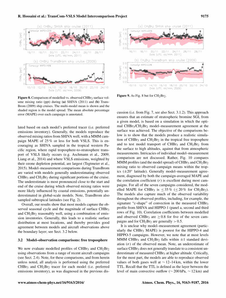
For the five models that submitted hourly output overthe period of the SHIVA (2011) and TransBrom (2009)ship cruises, Figs. 8 and 9 compare the multi-model mean(MMM) CHBr3 and CH2Br2 mixing ratio (and the modelspread) to the observed values. Note, the MMM was calcu-
Atmos. Chem. Phys., 16, 9163–9187, 2016 www.atmos-chem-phys.net/16/9163/2016/
R. Hossaini et al.: TransCom-VSLS Model Intercomparison Project 9175
Figure 8. Comparison of modelled vs. observed CHBr3 surface vol-ume mixing ratio (ppt) during (a) SHIVA (2011) and (b) Trans-Brom (2009) ship cruises. The multi-model mean is shown and theshaded region is the model spread. The mean absolute percentageerror (MAPE) over each campaign is annotated.
lated based on each model’s preferred tracer (i.e. preferredemissions inventory). Generally, the models reproduce theobserved mixing ratios from SHIVA well, with a MMM cam-paign MAPE of 25 % or less for both VSLS. This is en-couraging as SHIVA sampled in the tropical western Pa-cific region, where rapid troposphere-to-stratosphere trans-port of VSLS likely occurs (e.g. Aschmann et al., 2009;Liang et al., 2014) and where VSLS emissions, weighted bytheir ozone depletion potential, are largest (Tegtmeier et al.,2015). Model–measurement comparisons during TransBromare varied with models generally underestimating observedCHBr3 and CH2Br2 during significant portions of the cruise.The underestimate is most pronounced close to the start andend of the cruise during which observed mixing ratios weremore likely influenced by coastal emissions, potentially un-derestimated in global-scale models. Note, TransBrom alsosampled subtropical latitudes (see Fig. 2).
Overall, our results show that most models capture the ob-served seasonal cycle and the magnitude of surface CHBr3and CH2Br2 reasonably well, using a combination of emis-sion inventories. Generally, this leads to a realistic surfacedistribution at most locations, and thereby provides goodagreement between models and aircraft observations abovethe boundary layer; see Sect. 3.2 below.
3.2 Model–observation comparisons: free troposphere
We now evaluate modelled profiles of CHBr3 and CH2Br2using observations from a range of recent aircraft campaigns(see Sect. 2.4). Note, for these comparisons, and from hereinunless noted, all analysis is performed using the preferredCHBr3 and CH2Br2 tracer for each model (i.e. preferredemissions inventory), as was diagnosed in the previous dis-
Figure 9. As Fig. 8 but for CH2Br2.
cussion (i.e. from Fig. 7, see also Sect. 3.1.2). This approachensures that an estimate of stratospheric bromine SGI, froma given model, is based on a simulation in which the opti-mal CHBr3/CH2Br2 model–measurement agreement at thesurface was achieved. The objective of the comparisons be-low is to show that the models produce a realistic simula-tion of CHBr3 and CH2Br2 in the tropical free troposphereand to test model transport of CHBr3 and CH2Br2 fromthe surface to high altitudes, against that from atmosphericmeasurements. Intricacies of individual model–measurementcomparison are not discussed. Rather, Fig. 10 comparesMMM profiles (and the model spread) of CHBr3 and CH2Br2mixing ratio to observed campaign means within the trop-ics (±20◦ latitude). Generally model–measurement agree-ment, diagnosed by both the campaign-averaged MAPE andthe correlation coefficient (r) is excellent during most cam-paigns. For all of the seven campaigns considered, the mod-elled MAPE for CHBr3 is ≤ 35 % (≤ 20 % for CH2Br2).The models also capture much of the observed variabilitythroughout the observed profiles, including, for example, thesignature “c-shape” of convection in the measured CHBr3profile from SHIVA and HIPPO-1 (panel a, second and thirdrows of Fig. 10). Correlation coefficients between modelledand observed CHBr3 are ≥ 0.8 for five of the seven cam-paigns and for CH2Br2 are generally > 0.5.
It is unclear why model–measurement agreement (partic-ularly the CHBr3 MAPE) is poorest for the HIPPO-4 andHIPPO-5 campaigns. However, we note that at most levelsMMM CHBr3 and CH2Br2 falls within ±1 standard devi-ation (σ ) of the observed mean. Note, an underestimate ofsurface CHBr3 does not generally translate to a consistent un-derestimate of measured CHBr3 at higher altitude. Critically,for the most part, the models are able to reproduce observedvalues of both gases well at ∼ 12–14 km, within the lowerTTL. Recall that the TTL is defined as the layer between thelevel of main convective outflow (∼ 200 hPa, ∼ 12 km) and
www.atmos-chem-phys.net/16/9163/2016/ Atmos. Chem. Phys., 16, 9163–9187, 2016
9176 R. Hossaini et al.: TransCom-VSLS Model Intercomparison Project
(a) CHBr3
0.0 0.5 1.0 1.5 2.0
0
5
10
15A
ltitu
de
(km
) CA
ST
r = 0.96MAPE = 32 %
(b) CH2Br2
0.0 0.5 1.0 1.5 2.0
0
5
10
15
r = 0.81MAPE = 20 %
0.0 0.5 1.0 1.5 2.0
0
5
10
15
Altitu
de
(km
) SH
IVA
r = 0.84MAPE = 16 %
0.0 0.5 1.0 1.5 2.0
0
5
10
15
r = 0.84MAPE = 6 %
0.0 0.5 1.0 1.5 2.0
0
5
10
15
Altitu
de
(km
) HIP
PO
-1
r = 0.84MAPE = 20 %
0.0 0.5 1.0 1.5 2.0
0
5
10
15
r = 0.54MAPE = 7 %
0.0 0.5 1.0 1.5 2.0
0
5
10
15
Altitu
de
(km
) HIP
PO
-2
r = 0.65MAPE = 16 %
0.0 0.5 1.0 1.5 2.0
0
5
10
15
r = 0.73MAPE = 5 %
0.0 0.5 1.0 1.5 2.0
0
5
10
15
Altitu
de
(km
) HIP
PO
-3
r = 0.81MAPE = 14 %
0.0 0.5 1.0 1.5 2.0
0
5
10
15
r = 0.69MAPE = 5 %
0.0 0.5 1.0 1.5 2.0
0
5
10
15
Altitu
de
(km
) HIP
PO
-4r = 0.59
MAPE = 34 %
0.0 0.5 1.0 1.5 2.0
0
5
10
15
r = 0.43MAPE = 3 %
0.0 0.5 1.0 1.5 2.0
0
5
10
15
Altitu
de
(km
) HIP
PO
-5
r = 0.80MAPE = 33 %
0.0 0.5 1.0 1.5 2.0
0
5
10
15
r = 0.42MAPE = 13 %
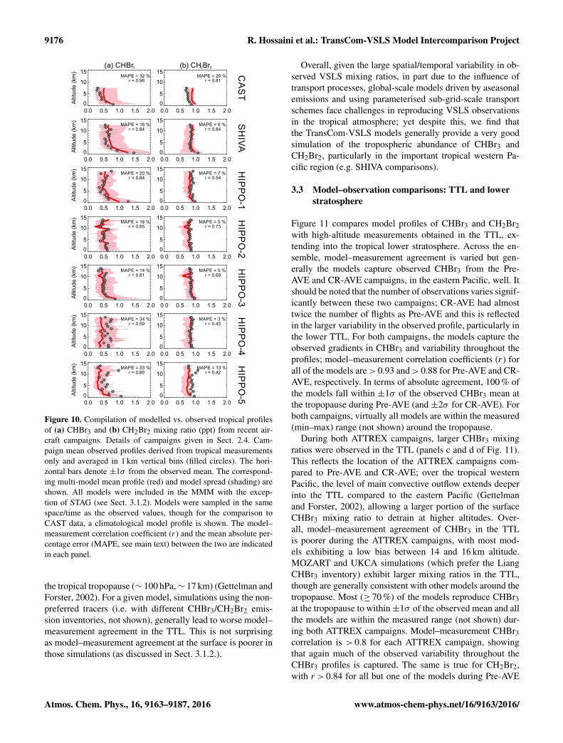
Figure 10. Compilation of modelled vs. observed tropical profilesof (a) CHBr3 and (b) CH2Br2 mixing ratio (ppt) from recent air-craft campaigns. Details of campaigns given in Sect. 2.4. Cam-paign mean observed profiles derived from tropical measurementsonly and averaged in 1 km vertical bins (filled circles). The hori-zontal bars denote ±1σ from the observed mean. The correspond-ing multi-model mean profile (red) and model spread (shading) areshown. All models were included in the MMM with the excep-tion of STAG (see Sect. 3.1.2). Models were sampled in the samespace/time as the observed values, though for the comparison toCAST data, a climatological model profile is shown. The model–measurement correlation coefficient (r) and the mean absolute per-centage error (MAPE, see main text) between the two are indicatedin each panel.
the tropical tropopause (∼ 100 hPa,∼ 17 km) (Gettelman andForster, 2002). For a given model, simulations using the non-preferred tracers (i.e. with different CHBr3/CH2Br2 emis-sion inventories, not shown), generally lead to worse model–measurement agreement in the TTL. This is not surprisingas model–measurement agreement at the surface is poorer inthose simulations (as discussed in Sect. 3.1.2.).
Overall, given the large spatial/temporal variability in ob-served VSLS mixing ratios, in part due to the influence oftransport processes, global-scale models driven by aseasonalemissions and using parameterised sub-grid-scale transportschemes face challenges in reproducing VSLS observationsin the tropical atmosphere; yet despite this, we find thatthe TransCom-VSLS models generally provide a very goodsimulation of the tropospheric abundance of CHBr3 andCH2Br2, particularly in the important tropical western Pa-cific region (e.g. SHIVA comparisons).
3.3 Model–observation comparisons: TTL and lowerstratosphere
Figure 11 compares model profiles of CHBr3 and CH2Br2with high-altitude measurements obtained in the TTL, ex-tending into the tropical lower stratosphere. Across the en-semble, model–measurement agreement is varied but gen-erally the models capture observed CHBr3 from the Pre-AVE and CR-AVE campaigns, in the eastern Pacific, well. Itshould be noted that the number of observations varies signif-icantly between these two campaigns; CR-AVE had almosttwice the number of flights as Pre-AVE and this is reflectedin the larger variability in the observed profile, particularly inthe lower TTL. For both campaigns, the models capture theobserved gradients in CHBr3 and variability throughout theprofiles; model–measurement correlation coefficients (r) forall of the models are> 0.93 and> 0.88 for Pre-AVE and CR-AVE, respectively. In terms of absolute agreement, 100 % ofthe models fall within ±1σ of the observed CHBr3 mean atthe tropopause during Pre-AVE (and ±2σ for CR-AVE). Forboth campaigns, virtually all models are within the measured(min–max) range (not shown) around the tropopause.
During both ATTREX campaigns, larger CHBr3 mixingratios were observed in the TTL (panels c and d of Fig. 11).This reflects the location of the ATTREX campaigns com-pared to Pre-AVE and CR-AVE; over the tropical westernPacific, the level of main convective outflow extends deeperinto the TTL compared to the eastern Pacific (Gettelmanand Forster, 2002), allowing a larger portion of the surfaceCHBr3 mixing ratio to detrain at higher altitudes. Over-all, model–measurement agreement of CHBr3 in the TTLis poorer during the ATTREX campaigns, with most mod-els exhibiting a low bias between 14 and 16 km altitude.MOZART and UKCA simulations (which prefer the LiangCHBr3 inventory) exhibit larger mixing ratios in the TTL,though are generally consistent with other models around thetropopause. Most (≥ 70 %) of the models reproduce CHBr3at the tropopause to within±1σ of the observed mean and allthe models are within the measured range (not shown) dur-ing both ATTREX campaigns. Model–measurement CHBr3correlation is > 0.8 for each ATTREX campaign, showingthat again much of the observed variability throughout theCHBr3 profiles is captured. The same is true for CH2Br2,with r > 0.84 for all but one of the models during Pre-AVE
Atmos. Chem. Phys., 16, 9163–9187, 2016 www.atmos-chem-phys.net/16/9163/2016/

R. Hossaini et al.: TransCom-VSLS Model Intercomparison Project 9177
0 0.2 0.4 0.6 0.8 1.0
12
14
16
18
20(a) CHBr3 PRE-AVE
0 0.2 0.4 0.6 0.8 1.0CHBr3 (ppt)
12
14
16
18
20
Altitude (
km
)
(b) CHBr3 CR-AVE
0 0.2 0.4 0.6 0.8 1.0CHBr3 (ppt)
(c) CHBr3 ATTREX 2013
0 0.2 0.4 0.6 0.8 1.0CHBr3 (ppt)
(d) CHBr3 ATTREX 2014
0 0.2 0.4 0.6 0.8 1.0CHBr3 (ppt)
(e) CH2Br2 PRE-AVE
0 0.3 0.6 0.9 1.2CH2Br2 (ppt)
12
14
16
18
20
Altitude (
km
)
(f) CH2Br2 CR-AVE
0 0.3 0.6 0.9 1.2CH2Br2 (ppt)
(g) CH2Br2 ATTREX 2013
0 0.3 0.6 0.9 1.2CH2Br2 (ppt)
(h) CH2Br2 ATTREX 2014
0 0.3 0.6 0.9 1.2CH2Br2 (ppt)
ACTM
B3DCTM
EMAC_F
EMAC_N
MOZART
NIES-TM
TOMCAT
TOMCAT_CONV
UKCA_LO
UKCA_HI
Figure 11. Comparison of modelled vs. observed volume mixing ratio (ppt) of CHBr3 (a–d) and CH2Br2 (e–h) from aircraft campaignsin the tropics (see main text for campaign details). The observed values (filled circles) are averages in 1 km altitude bins and the error barsdenote ±1σ . The dashed line denotes the approximate cold point tropopause for reference.
and r > 0.88 for all of the models in each of the other cam-paigns.
Overall, mean CHBr3 and CH2Br2 mixing ratios aroundthe tropopause, observed during the 2013/2014 ATTREXmissions, are larger than the mean mixing ratios (from pre-vious aircraft campaigns) reported in the latest WMO OzoneAssessment Report (Tables 1–7 of Carpenter and Reimann,2014). As noted, this likely reflects the location at which themeasurements were made; ATTREX 2013/2014 sampled inthe tropical West and central Pacific, whereas the WMO es-timate is based on a compilation of measurements with apaucity in that region. From Fig. 11, observed CHBr3 andCH2Br2 at the tropopause were (on average) ∼ 0.35 ppt and∼ 0.8 ppt, respectively, during ATTREX 2013/2014, com-pared to the 0.08 (0.00–0.31) ppt CHBr3 and 0.52 (0.3–0.86) ppt CH2Br2 ranges reported by Carpenter and Reimann(2014).
3.4 Seasonal and zonal variations in thetroposphere-to-stratosphere transport of VSLS
In this section we examine seasonal and zonal variability inthe loading of CHBr3 and CH2Br2 in the TTL and lowerstratosphere, indicative of transport processes. In the trop-ics, a number of previous studies have shown a marked sea-sonality in convective outflow around the tropopause, owingto seasonal variations in convective cloud top heights (e.g.Folkins et al., 2006; Hosking et al., 2010; Bergman et al.,2012). Such variations influence the near-tropopause abun-dance of brominated VSLS (Hoyle et al., 2011; Liang et al.,2014) and other tracers, such as CO (Folkins et al., 2006).
Figures 12 and 13 show the simulated seasonal cycle ofCHBr3 and CH2Br2, respectively, at the base of the TTLand the cold point tropopause (CPT). CHBr3 exhibits a pro-nounced seasonal cycle at the CPT, with virtually all modelsshowing the same phase; with respect to the annual mean andintegrated over the tropics, CHBr3 is most elevated duringboreal winter (DJF). The amplitude of the cycle varies con-siderably between models, with departures from the annualmean ranging from around ±10 to ±40 %, in a given month(panel b of Fig. 12). Owing to its relatively long troposphericlifetime, particularly in the TTL (> 1 year) (Hossaini et al.,2010), CH2Br2 exhibits a weak seasonal cycle at the CPT asit is less influenced by seasonal variations in transport.
Panels c and d of Figs. 12 and 13, also show the modelledabsolute mixing ratios of CHBr3 and CH2Br2 at the TTLbase and CPT. Annually averaged, for CHBr3, the modelspread results in a factor of ∼ 3 difference in simulatedCHBr3 at both levels (similarly, for CH2Br2 a factor of 1.5).The modelled mixing ratios fall within the measurement-derived range reported by Carpenter and Reimann (2014).The MMM CHBr3 mixing ratio at the TTL base is 0.51 ppt,within the 0.2–1.1 ppt measurement-derived range. At theCPT, the MMM CHBr3 mixing ratio is 0.20 ppt, also withinthe measured range of 0.0–0.31 ppt. On average, the modelssuggest a ∼ 60 % gradient in CHBr3 between the TTL baseand tropopause. Similarly, the annual MMM CH2Br2 mixingratio is 0.82 ppt at the TTL base, within the measured rangeof 0.6–1.2 ppt, and at the CPT is 0.73 ppt, within the mea-sured range of 0.3–0.86 ppt. On average, the models showa CH2Br2 gradient of 10 % between the two levels. Thesemodel absolute values are annual means over the whole
www.atmos-chem-phys.net/16/9163/2016/ Atmos. Chem. Phys., 16, 9163–9187, 2016

9178 R. Hossaini et al.: TransCom-VSLS Model Intercomparison Project
200 hPa (TTL base)
0 2 4 6 8 10 12-30-20
-10
0
10
2030
Ano
mal
y (%
)
(a)
100 hPa (CPT)
0 2 4 6 8 10 12
-40
-20
0
20
40
(b)
0 2 4 6 8 10 12Month
0.00.2
0.4
0.6
0.8
1.01.2
CH
Br 3
(ppt
)
(c)
0 2 4 6 8 10 12Month
0.0
0.2
0.4
0.6
(d)
Figure 12. Simulated monthly mean anomalies of CHBr3 volumemixing ratio (vmr), expressed as a percentage with respect to theannual mean, for (a) 200 hPa, the approximate base of the tropicaltropopause layer (TTL) and (b) 100 hPa, the cold point tropopause(CPT). Panels (c, d) show the CHBr3 vmr (ppt) at these levels. Allpanels show tropical (±20◦ latitude) averages over the full simula-tion period (1993–2012). See Fig. 3 for legend. The thick black linedenotes the multi-model mean.
200 hPa (TTL base)
0 2 4 6 8 10 12-15-10
-5
0
5
1015
Ano
mal
y (%
)
(a)
100 hPa (CPT)
0 2 4 6 8 10 12-15-10
-5
0
5
1015
(b)
0 2 4 6 8 10 12Month
0.0
0.5
1.0
1.5
CH
2Br 2
(ppt
)
(c)
0 2 4 6 8 10 12Month
0.0
0.5
1.0
1.5
(d)
Figure 13. As Fig. 12 but for CH2Br2.
tropical domain. However, zonal variability in VSLS load-ing within the TTL is expected to be large (e.g. Aschmannet al., 2009; Liang et al., 2014), owing to inhomogeneityin the spatial distribution of convection and oceanic emis-sions. The Indian Ocean, the Maritime Continent (incorpo-rating Malaysia, Indonesia, and the surrounding islands andocean), central America, and central Africa are all convec-tively active regions, shown to experience particularly deepconvective events, with the potential, therefore, to rapidly loftVSLS from the surface into the TTL (e.g. Gettelman et al.,2002, 2009; Hosking et al., 2010). As previously noted, theabsolute values can vary, though generally the TransCom-VSLS models agree on the locations with the highest VSLSmixing ratios, as seen from the zonal CHBr3 anomalies atthe CPT shown in Fig. 14. These regions are consistent withthe convective source regions discussed above. The largest
DJF JJAA
CT
MB
3D
CT
ME
MA
C_
FE
MA
C_
NM
OZ
AR
TN
IES
-TM
ST
AG
TO
MC
AT
TO
MC
AT
_C
UK
CA
_L
UK
CA
_H
-100 0 100
CHBr3 anom ly (%)a
Figure 14. Simulated anomalies of the CHBr3 volume mixing ratiowith respect to the tropical (±30◦ latitude) mean (expressed in %)at 100 hPa for (a) boreal winter (DJF) and (b) boreal summer (JJA).The boxes highlight the tropical western Pacific and location of theAsian monsoon – regions experiencing strong convection.
CHBr3 mixing ratios at the CPT are predicted over the trop-ical western Pacific (20◦ S–20◦ N, 100–180◦ E), particularlyduring DJF. Integrated over the tropical domain, this signalexerts the largest influence on the CHBr3 seasonal cycle atthe CPT. This result is consistent with the model intercom-parison of Hoyle et al. (2011), who examined the seasonalcycle of idealised VSLS-like tracers around the tropopause,and reported a similar seasonality.
While meridionally, the width of elevated CHBr3 mixingratios during DJF is similar across the models, differences
Atmos. Chem. Phys., 16, 9163–9187, 2016 www.atmos-chem-phys.net/16/9163/2016/
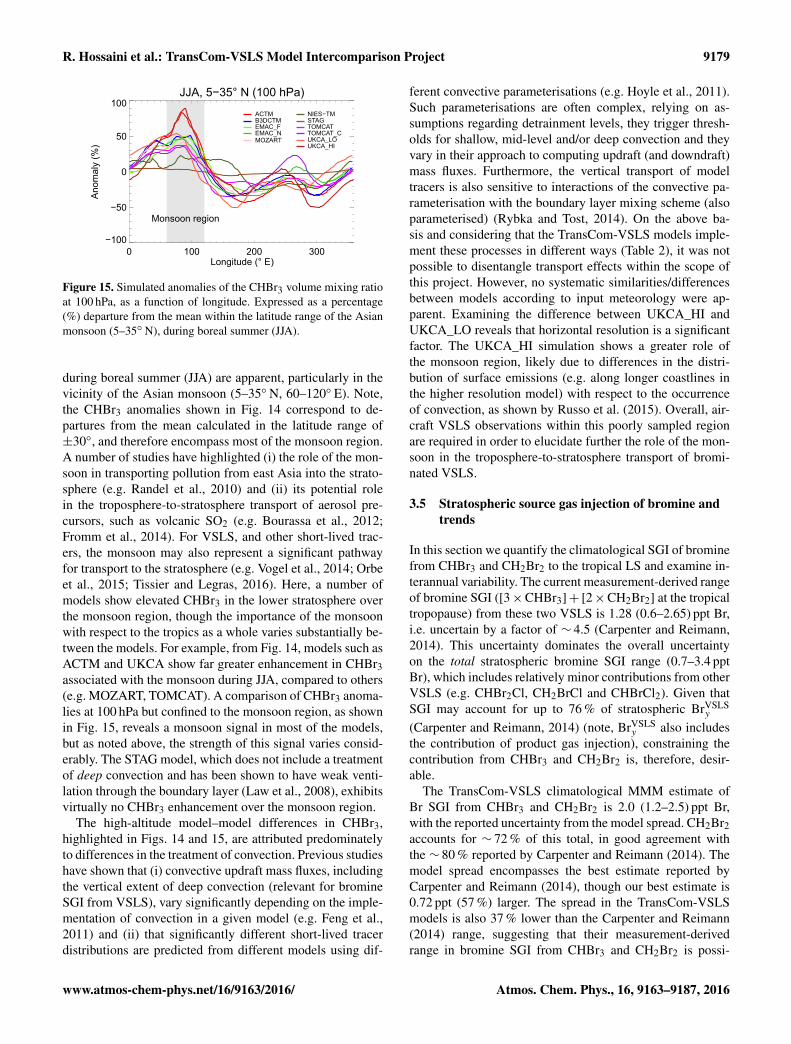
R. Hossaini et al.: TransCom-VSLS Model Intercomparison Project 9179
JJA, 5−35° N (100 hPa)
0 100 200 300Longitude (° E)
−100
−50
0
50
100A
nom
aly
(%
)
Monsoon region
ACTMB3DCTMEMAC_FEMAC_NMOZART
NIES−TMSTAGTOMCATTOMCAT_CUKCA_LOUKCA_HI
Figure 15. Simulated anomalies of the CHBr3 volume mixing ratioat 100 hPa, as a function of longitude. Expressed as a percentage(%) departure from the mean within the latitude range of the Asianmonsoon (5–35◦ N), during boreal summer (JJA).
during boreal summer (JJA) are apparent, particularly in thevicinity of the Asian monsoon (5–35◦ N, 60–120◦ E). Note,the CHBr3 anomalies shown in Fig. 14 correspond to de-partures from the mean calculated in the latitude range of±30◦, and therefore encompass most of the monsoon region.A number of studies have highlighted (i) the role of the mon-soon in transporting pollution from east Asia into the strato-sphere (e.g. Randel et al., 2010) and (ii) its potential rolein the troposphere-to-stratosphere transport of aerosol pre-cursors, such as volcanic SO2 (e.g. Bourassa et al., 2012;Fromm et al., 2014). For VSLS, and other short-lived trac-ers, the monsoon may also represent a significant pathwayfor transport to the stratosphere (e.g. Vogel et al., 2014; Orbeet al., 2015; Tissier and Legras, 2016). Here, a number ofmodels show elevated CHBr3 in the lower stratosphere overthe monsoon region, though the importance of the monsoonwith respect to the tropics as a whole varies substantially be-tween the models. For example, from Fig. 14, models such asACTM and UKCA show far greater enhancement in CHBr3associated with the monsoon during JJA, compared to others(e.g. MOZART, TOMCAT). A comparison of CHBr3 anoma-lies at 100 hPa but confined to the monsoon region, as shownin Fig. 15, reveals a monsoon signal in most of the models,but as noted above, the strength of this signal varies consid-erably. The STAG model, which does not include a treatmentof deep convection and has been shown to have weak venti-lation through the boundary layer (Law et al., 2008), exhibitsvirtually no CHBr3 enhancement over the monsoon region.
The high-altitude model–model differences in CHBr3,highlighted in Figs. 14 and 15, are attributed predominatelyto differences in the treatment of convection. Previous studieshave shown that (i) convective updraft mass fluxes, includingthe vertical extent of deep convection (relevant for bromineSGI from VSLS), vary significantly depending on the imple-mentation of convection in a given model (e.g. Feng et al.,2011) and (ii) that significantly different short-lived tracerdistributions are predicted from different models using dif-
ferent convective parameterisations (e.g. Hoyle et al., 2011).Such parameterisations are often complex, relying on as-sumptions regarding detrainment levels, they trigger thresh-olds for shallow, mid-level and/or deep convection and theyvary in their approach to computing updraft (and downdraft)mass fluxes. Furthermore, the vertical transport of modeltracers is also sensitive to interactions of the convective pa-rameterisation with the boundary layer mixing scheme (alsoparameterised) (Rybka and Tost, 2014). On the above ba-sis and considering that the TransCom-VSLS models imple-ment these processes in different ways (Table 2), it was notpossible to disentangle transport effects within the scope ofthis project. However, no systematic similarities/differencesbetween models according to input meteorology were ap-parent. Examining the difference between UKCA_HI andUKCA_LO reveals that horizontal resolution is a significantfactor. The UKCA_HI simulation shows a greater role ofthe monsoon region, likely due to differences in the distri-bution of surface emissions (e.g. along longer coastlines inthe higher resolution model) with respect to the occurrenceof convection, as shown by Russo et al. (2015). Overall, air-craft VSLS observations within this poorly sampled regionare required in order to elucidate further the role of the mon-soon in the troposphere-to-stratosphere transport of bromi-nated VSLS.
3.5 Stratospheric source gas injection of bromine andtrends
In this section we quantify the climatological SGI of brominefrom CHBr3 and CH2Br2 to the tropical LS and examine in-terannual variability. The current measurement-derived rangeof bromine SGI ([3×CHBr3]+ [2×CH2Br2] at the tropicaltropopause) from these two VSLS is 1.28 (0.6–2.65) ppt Br,i.e. uncertain by a factor of ∼ 4.5 (Carpenter and Reimann,2014). This uncertainty dominates the overall uncertaintyon the total stratospheric bromine SGI range (0.7–3.4 pptBr), which includes relatively minor contributions from otherVSLS (e.g. CHBr2Cl, CH2BrCl and CHBrCl2). Given thatSGI may account for up to 76 % of stratospheric BrVSLS
y
(Carpenter and Reimann, 2014) (note, BrVSLSy also includes
the contribution of product gas injection), constraining thecontribution from CHBr3 and CH2Br2 is, therefore, desir-able.
The TransCom-VSLS climatological MMM estimate ofBr SGI from CHBr3 and CH2Br2 is 2.0 (1.2–2.5) ppt Br,with the reported uncertainty from the model spread. CH2Br2accounts for ∼ 72 % of this total, in good agreement withthe ∼ 80 % reported by Carpenter and Reimann (2014). Themodel spread encompasses the best estimate reported byCarpenter and Reimann (2014), though our best estimate is0.72 ppt (57 %) larger. The spread in the TransCom-VSLSmodels is also 37 % lower than the Carpenter and Reimann(2014) range, suggesting that their measurement-derivedrange in bromine SGI from CHBr3 and CH2Br2 is possi-
www.atmos-chem-phys.net/16/9163/2016/ Atmos. Chem. Phys., 16, 9163–9187, 2016
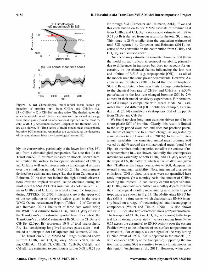
9180 R. Hossaini et al.: TransCom-VSLS Model Intercomparison Project
(a) Climatologicalmulti-model mean Br SGI
0 1 2 3 4 5Bromine (ppt)
1000
100
Pre
ssure
(hP
a)
TTL base
Tropopause
WMO range
(b) SGI annual mean time series
1995 2000 2005 2010Year
-10
-5
0
5
10
Anom
aly
(%
)
Figure 16. (a) Climatological multi-model mean source gasinjection of bromine (ppt) from CHBr3 and CH2Br2 (i.e.[3×CHBr3]+ [2×CH2Br2] mixing ratio). The shaded region de-notes the model spread. The best estimate (red circle) and SGI rangefrom these gases (based on observations) reported in the most re-cent WMO O3 Assessment Report (Carpenter and Reimann, 2014)are also shown. (b) Time series of multi-model mean stratosphericbromine SGI anomalies. Anomalies are calculated as the departureof the annual mean from the climatological mean (%).
bly too conservative, particularly at the lower limit (Fig. 16),and from a climatological perspective. We note that (i) theTransCom-VSLS estimate is based on models, shown here,to simulate the surface to tropopause abundance of CHBr3and CH2Br2 well and (ii) represents a climatological estimateover the simulation period, 1995–2012. The measurement-derived best estimate and range (i.e. that from Carpenter andReimann, 2014) does not include the high-altitude observa-tions over the tropical western Pacific obtained during themost recent NASA ATTREX missions. As noted in Sect. 3.3,mean CHBr3 and CH2Br2 measured around the tropopauseduring ATTREX (2013/2014 missions), are at the upper endof the compilation of observed values given in the recentWMO Ozone Assessment Report (Tables 1–7 of Carpenterand Reimann, 2014). Inclusion of these data would bringthe WMO SGI estimate from CHBr3 and CH2Br2 closer tothe TransCom-VSLS estimate reported here. For context, theTransCom-VSLS MMM estimate of Br SGI from CHBr3 andCH2Br2 (2.0 ppt Br) represents 10 % of total stratosphericBry (i.e. considering long-lived sources gases also) – esti-mated at ∼ 20 ppt in 2011 (Carpenter and Reimann, 2014).
The TransCom-VSLS MMM SGI range discussed aboveis from CHBr3 and CH2Br2 only. Minor VSLS, includ-ing CHBr2Cl, CH2BrCl, CHBrCl2, C2H5Br, C2H4Br andC3H7Br, are estimated to contribute a further 0.08 to 0.71 ppt
Br through SGI (Carpenter and Reimann, 2014). If we addthis contribution on to our MMM estimate of bromine SGIfrom CHBr3 and CH2Br2, a reasonable estimate of 1.28 to3.21 ppt Br is derived from our results for the total SGI range.This range is 28 % smaller than the equivalent estimate oftotal SGI reported by Carpenter and Reimann (2014), be-cause of the constraint on the contribution from CHBr3 andCH2Br2, as discussed above.
Our uncertainty estimate on simulated bromine SGI (fromthe model spread) reflects inter-model variability, primarilydue to differences in transport, but does not account for un-certainty on the chemical factors influencing the loss rateand lifetime of VSLS (e.g. tropospheric [OH]) – as all ofthe models used the same prescribed oxidants. However, As-chmann and Sinnhuber (2013) found that the stratosphericSGI of Br exhibited a low sensitivity to large perturbationsto the chemical loss rate of CHBr3 and CH2Br2; a ±50 %perturbation to the loss rate changed bromine SGI by 2 %at most in their model sensitivity experiments. Furthermore,our SGI range is compatible with recent model SGI esti-mates that used different [OH] fields; for example, Fernan-dez et al. (2014) simulated a stratospheric SGI of 1.7 ppt Brfrom CHBr3 and CH2Br2.
We found no clear long-term transport-driven trend in thestratospheric SGI of bromine. Clearly, this result is limitedto the study period examined and does not preclude poten-tial future changes due to climate change, as suggested bysome studies (e.g. Hossaini et al., 2012b). In terms of inter-annual variability, the simulated annual mean bromine SGIvaried by ±5 % around the climatological mean (panel b ofFig. 16) over the simulation period (small in the context of to-tal stratospheric Bry , see above). Naturally, this encompassesinterannual variability of both CHBr3 and CH2Br2 reachingthe tropical LS, the latter of which is far smaller, and giventhat CH2Br2 is the larger contributor to SGI, dampens theoverall interannual variability. Note, interannual changes inemissions, [OH] or photolysis rates were not quantified here(only transport). On a monthly basis, the amount of CHBr3reaching the tropical LS can clearly exhibit larger variabil-ity. CHBr3 anomalies (calculated as monthly departures fromthe climatological monthly mean mixing ratio) at the tropicaltropopause are shown in Fig. 17. The Multivariate ENSO In-dex (MEI) – a time series which characterises ENSO inten-sity based on a range of meteorological and oceanographiccomponents (Wolter and Timlin, 1998) – is also shownin Fig. 17. See also http://www.esrl.noaa.gov/psd/enso/mei/.The transport of CHBr3 (and CH2Br2, not shown) to the trop-ical LS is strongly correlated (r values ranging from 0.6 to0.75 across the ensemble) to ENSO activity over the easternPacific (owing to the influence of sea surface temperature onconvection). For example, a clear signal of the very strongEl Niño event of 1997/1998 is apparent in the models (i.e.with enhanced CHBr3 at the tropopause) supporting the no-tion that bromine SGI is sensitive to such climate modes, inthis region (Aschmann et al., 2011). However, when aver-
Atmos. Chem. Phys., 16, 9163–9187, 2016 www.atmos-chem-phys.net/16/9163/2016/
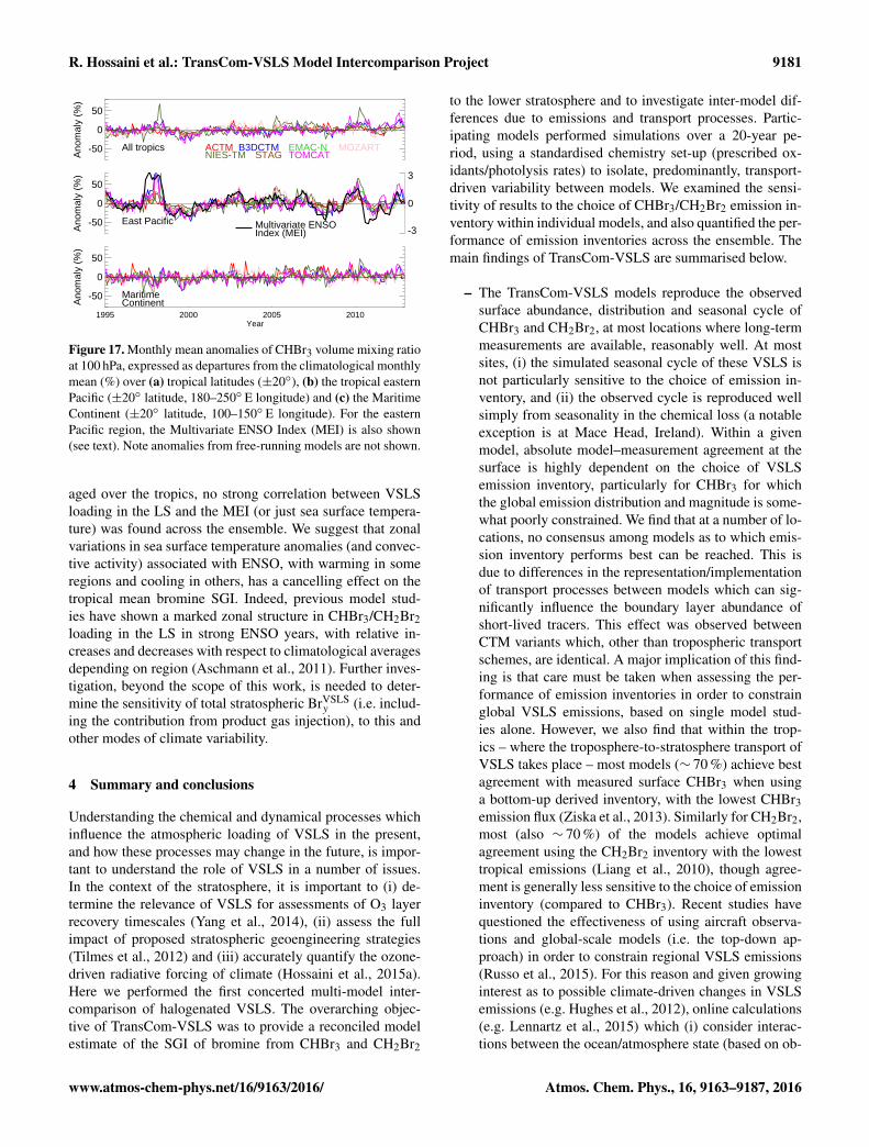
R. Hossaini et al.: TransCom-VSLS Model Intercomparison Project 9181
-50
0
50
Ano
mal
y (%
)
All tropics ACTM B3DCTM EMAC-N MOZARTNIES-TM STAG TOMCAT
-50
0
50
Ano
mal
y (%
)
East Pacific Multivariate ENSO Index (MEI) -3
0
3
ME
I
-50
0
50
Ano
mal
y (%
)
Maritime Continent
1995 2000 2005 2010Year
Figure 17. Monthly mean anomalies of CHBr3 volume mixing ratioat 100 hPa, expressed as departures from the climatological monthlymean (%) over (a) tropical latitudes (±20◦), (b) the tropical easternPacific (±20◦ latitude, 180–250◦ E longitude) and (c) the MaritimeContinent (±20◦ latitude, 100–150◦ E longitude). For the easternPacific region, the Multivariate ENSO Index (MEI) is also shown(see text). Note anomalies from free-running models are not shown.
aged over the tropics, no strong correlation between VSLSloading in the LS and the MEI (or just sea surface tempera-ture) was found across the ensemble. We suggest that zonalvariations in sea surface temperature anomalies (and convec-tive activity) associated with ENSO, with warming in someregions and cooling in others, has a cancelling effect on thetropical mean bromine SGI. Indeed, previous model stud-ies have shown a marked zonal structure in CHBr3/CH2Br2loading in the LS in strong ENSO years, with relative in-creases and decreases with respect to climatological averagesdepending on region (Aschmann et al., 2011). Further inves-tigation, beyond the scope of this work, is needed to deter-mine the sensitivity of total stratospheric BrVSLS
y (i.e. includ-ing the contribution from product gas injection), to this andother modes of climate variability.
4 Summary and conclusions
Understanding the chemical and dynamical processes whichinfluence the atmospheric loading of VSLS in the present,and how these processes may change in the future, is impor-tant to understand the role of VSLS in a number of issues.In the context of the stratosphere, it is important to (i) de-termine the relevance of VSLS for assessments of O3 layerrecovery timescales (Yang et al., 2014), (ii) assess the fullimpact of proposed stratospheric geoengineering strategies(Tilmes et al., 2012) and (iii) accurately quantify the ozone-driven radiative forcing of climate (Hossaini et al., 2015a).Here we performed the first concerted multi-model inter-comparison of halogenated VSLS. The overarching objec-tive of TransCom-VSLS was to provide a reconciled modelestimate of the SGI of bromine from CHBr3 and CH2Br2
to the lower stratosphere and to investigate inter-model dif-ferences due to emissions and transport processes. Partic-ipating models performed simulations over a 20-year pe-riod, using a standardised chemistry set-up (prescribed ox-idants/photolysis rates) to isolate, predominantly, transport-driven variability between models. We examined the sensi-tivity of results to the choice of CHBr3/CH2Br2 emission in-ventory within individual models, and also quantified the per-formance of emission inventories across the ensemble. Themain findings of TransCom-VSLS are summarised below.
– The TransCom-VSLS models reproduce the observedsurface abundance, distribution and seasonal cycle ofCHBr3 and CH2Br2, at most locations where long-termmeasurements are available, reasonably well. At mostsites, (i) the simulated seasonal cycle of these VSLS isnot particularly sensitive to the choice of emission in-ventory, and (ii) the observed cycle is reproduced wellsimply from seasonality in the chemical loss (a notableexception is at Mace Head, Ireland). Within a givenmodel, absolute model–measurement agreement at thesurface is highly dependent on the choice of VSLSemission inventory, particularly for CHBr3 for whichthe global emission distribution and magnitude is some-what poorly constrained. We find that at a number of lo-cations, no consensus among models as to which emis-sion inventory performs best can be reached. This isdue to differences in the representation/implementationof transport processes between models which can sig-nificantly influence the boundary layer abundance ofshort-lived tracers. This effect was observed betweenCTM variants which, other than tropospheric transportschemes, are identical. A major implication of this find-ing is that care must be taken when assessing the per-formance of emission inventories in order to constrainglobal VSLS emissions, based on single model stud-ies alone. However, we also find that within the trop-ics – where the troposphere-to-stratosphere transport ofVSLS takes place – most models (∼ 70 %) achieve bestagreement with measured surface CHBr3 when usinga bottom-up derived inventory, with the lowest CHBr3emission flux (Ziska et al., 2013). Similarly for CH2Br2,most (also ∼ 70 %) of the models achieve optimalagreement using the CH2Br2 inventory with the lowesttropical emissions (Liang et al., 2010), though agree-ment is generally less sensitive to the choice of emissioninventory (compared to CHBr3). Recent studies havequestioned the effectiveness of using aircraft observa-tions and global-scale models (i.e. the top-down ap-proach) in order to constrain regional VSLS emissions(Russo et al., 2015). For this reason and given growinginterest as to possible climate-driven changes in VSLSemissions (e.g. Hughes et al., 2012), online calculations(e.g. Lennartz et al., 2015) which (i) consider interac-tions between the ocean/atmosphere state (based on ob-
www.atmos-chem-phys.net/16/9163/2016/ Atmos. Chem. Phys., 16, 9163–9187, 2016
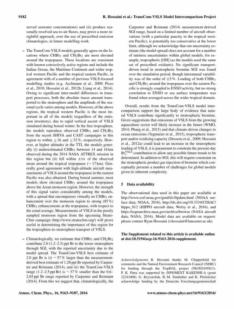
9182 R. Hossaini et al.: TransCom-VSLS Model Intercomparison Project
served seawater concentrations) and (ii) produce sea-sonally resolved sea-to-air fluxes, may prove a more in-sightful approach, over the use of prescribed emissionclimatologies, in future modelling work.
– The TransCom-VSLS models generally agree on the lo-cations where CHBr3 and CH2Br2 are most elevatedaround the tropopause. These locations are consistentwith known convectively active regions and include theIndian Ocean, the Maritime Continent and wider trop-ical western Pacific and the tropical eastern Pacific, inagreement with of a number of previous VSLS-focusedmodelling studies (e.g. Aschmann et al., 2009; Pissoet al., 2010; Hossaini et al., 2012b; Liang et al., 2014).Owing to significant inter-model differences in trans-port processes, both the absolute tracer amount trans-ported to the stratosphere and the amplitude of the sea-sonal cycle varies among models. However, of the aboveregions, the tropical western Pacific is the most im-portant in all of the models (regardless of the emis-sion inventory), due to rapid vertical ascent of VSLSsimulated during boreal winter. In the free troposphere,the models reproduce observed CHBr3 and CH2Br2from the recent SHIVA and CAST campaigns in thisregion to within ≤ 16 and ≤ 32 %, respectively. How-ever, at higher altitudes in the TTL the models gener-ally (i) underestimated CHBr3 between 14 and 16 kmobserved during the 2014 NASA ATTREX mission inthis region but (ii) fell within ±1σ of the observedmean around the tropical tropopause (∼ 17 km). Gen-erally good agreement with high-altitude aircraft mea-surements of VSLS around the tropopause in the easternPacific was also obtained. During boreal summer, mostmodels show elevated CHBr3 around the tropopauseabove the Asian monsoon region. However, the strengthof this signal varies considerably among the models,with a spread that encompasses virtually no CHBr3 en-hancement over the monsoon region to strong (85 %)CHBr3 enhancements at the tropopause, with respect tothe zonal average. Measurements of VSLS in the poorlysampled monsoon region from the upcoming Strato-Clim campaign (http://www.stratoclim.org/) will proveuseful in determining the importance of this region forthe troposphere-to-stratosphere transport of VSLS.
– Climatologically, we estimate that CHBr3 and CH2Br2contribute 2.0 (1.2–2.5) ppt Br to the lower stratospherethrough SGI, with the reported uncertainty due to themodel spread. The TransCom-VSLS best estimate of2.0 ppt Br is (i) ∼ 57 % larger than the measurement-derived best estimate of 1.28 ppt Br reported by Carpen-ter and Reimann (2014), and (ii) the TransCom-VSLSrange (1.2–2.5 ppt Br) is ∼ 37 % smaller than the 0.6–2.65 ppt Br range reported by Carpenter and Reimann(2014). From this we suggest that, climatologically, the
Carpenter and Reimann (2014) measurement-derivedSGI range, based on a limited number of aircraft obser-vations (with a particular paucity in the tropical west-ern Pacific), is potentially too conservative at the lowerlimit, although we acknowledge that our uncertainty es-timate (the model spread) does not account for a numberof intrinsic uncertainties within global models, for ex-ample, tropospheric [OH] (as the models used the sameset of prescribed oxidants). No significant transport-driven trend in stratospheric bromine SGI was foundover the simulation period, though interannual variabil-ity was of the order of ±5 %. Loading of both CHBr3and CH2Br2 around the tropopause over the eastern Pa-cific is strongly coupled to ENSO activity, but no strongcorrelation to ENSO or sea surface temperature wasfound when averaged across the wider tropical domain.
Overall, results from the TransCom-VSLS model inter-comparison support the large body of evidence that natu-ral VSLS contribute significantly to stratospheric bromine.Given suggestions that emissions of VSLS from the growingaquaculture sector will likely increase in the future (WMO,2014; Phang et al., 2015) and that climate-driven changes toocean emissions (Tegtmeier et al., 2015), tropospheric trans-port and/or oxidising capacity (Dessens et al., 2009; Hossainiet al., 2012a) could lead to an increase in the stratosphericloading of VSLS, it is paramount to constrain the present-dayBrVSLSy contribution to allow any possible future trends to be
determined. In addition to SGI, this will require constraint onthe stratospheric product gas injection of bromine which con-ceptually presents a number of challenges for global modelsgiven its inherent complexity.
5 Data availability
The observational data used in this paper are available athttp://www.esrl.noaa.gov/gmd/dv/ftpdata.html (NOAA sur-face data; NOAA, 2016), http://dx.doi.org/10.3334/CDIAC/hippo_012 (HIPPO aircraft data; Wofsy et al., 2016), andhttps://espoarchive.nasa.gov/archive/browse (NASA aircraftdata; NASA, 2016). Model data are available on request:please contact Ryan Hossaini ([email protected]).
The Supplement related to this article is available onlineat doi:10.5194/acp-16-9163-2016-supplement.
Acknowledgements. R. Hossaini thanks M. Chipperfield forcomments and the Natural Environment Research Council (NERC)for funding through the TropHAL project (NE/J02449X/1).P. K. Patra was supported by JSPS/MEXT KAKENHI-A (grant22241008). G. Krysztofiak, B.-M. Sinnhuber and K. Pfeilstickeracknowledge funding by the Deutsche Forschungsgemeinschaft
Atmos. Chem. Phys., 16, 9163–9187, 2016 www.atmos-chem-phys.net/16/9163/2016/
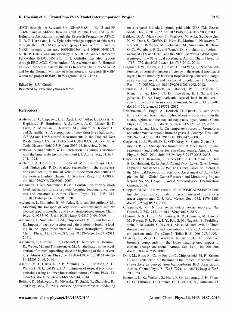
R. Hossaini et al.: TransCom-VSLS Model Intercomparison Project 9183
(DFG) through the Research Unit SHARP (SI 1400/1-2 and PF384/9-1 and in addition through grant PF 384/12-1) and by theHelmholtz Association through the Research Programme ATMO.N. R. P. Harris and J. A. Pyle acknowledge support of this workthrough the ERC ACCI project (project no. 267760), and byNERC through grant nos. NE/J006246/1 and NE/F1016012/1.N. R. P. Harris was supported by a NERC Advanced ResearchFellowship (NE/G014655/1). P. T. Griffiths was also supportthrough ERC ACCI. Contribution of J. Aschmann and R. Hommelhas been funded in part by the DFG Research Unit 1095 SHARP,and by the German Ministry of Education and Research (BMBF)within the project ROMIC-ROSA (grant 01LG1212A).
Edited by: J.-U. GrooßReviewed by: two anonymous referees
References
Andrews, S. J., Carpenter, L. J., Apel, E. C., Atlas, E., Donets, V.,Hopkins, J. F., Hornbrook, R. S., Lewis, A. C., Lidster, R. T.,Lueb, R., Minaeian, J., Navarro, M., Punjabi, S., Riemer, D.,and Schauffler, S.: A comparison of very short-lived halocarbon(VSLS) and DMS aircraft measurements in the Tropical WestPacific from CAST, ATTREX and CONTRAST, Atmos. Meas.Tech. Discuss., doi:10.5194/amt-2016-94, in review, 2016.
Arakawa, A. and Shubert, W. H.: Interaction of a cumulus ensemblewith the large-scale environment, Part I, J. Atmos. Sci., 31, 674–704, 1974.
Archer, S. D., Goldson, L. E., Liddicoat, M. I., Cummings, D. G.,and Nightingale, P. D.: Marked seasonality in the concentra-tions and sea-to-air flux of volatile iodocarbon compounds inthe western English Channel, J. Geophys. Res., 112, C08009,doi:10.1029/2006JC003963, 2007.
Aschmann, J. and Sinnhuber, B.-M.: Contribution of very short-lived substances to stratospheric bromine loading: uncertain-ties and constraints, Atmos. Chem. Phys., 13, 1203–1219,doi:10.5194/acp-13-1203-2013, 2013.
Aschmann, J., Sinnhuber, B.-M., Atlas, E. L., and Schauffler, S. M.:Modeling the transport of very short-lived substances into thetropical upper troposphere and lower stratosphere, Atmos. Chem.Phys., 9, 9237–9247, doi:10.5194/acp-9-9237-2009, 2009.
Aschmann, J., Sinnhuber, B.-M., Chipperfield, M. P., and Hossaini,R.: Impact of deep convection and dehydration on bromine load-ing in the upper troposphere and lower stratosphere, Atmos.Chem. Phys., 11, 2671–2687, doi:10.5194/acp-11-2671-2011,2011.
Aschmann, J., Burrows, J. P., Gebhardt, C., Rozanov, A., Hommel,R., Weber, M., and Thompson, A. M.: On the hiatus in the accel-eration of tropical upwelling since the beginning of the 21st cen-tury, Atmos. Chem. Phys., 14, 12803–12814, doi:10.5194/acp-14-12803-2014, 2014.
Ashfold, M. J., Harris, N. R. P., Manning, A. J., Robinson, A. D.,Warwick, N. J., and Pyle, J. A.: Estimates of tropical bromoformemissions using an inversion method, Atmos. Chem. Phys., 14,979–994, doi:10.5194/acp-14-979-2014, 2014.
Belikov, D., Maksyutov, S., Miyasaka, T., Saeki, T., Zhuravlev, R.,and Kiryushov, B.: Mass-conserving tracer transport modelling
on a reduced latitude-longitude grid with NIES-TM, Geosci.Model Dev., 4, 207–222, doi:10.5194/gmd-4-207-2011, 2011.
Belikov, D. A., Maksyutov, S., Sherlock, V., Aoki, S., Deutscher,N. M., Dohe, S., Griffith, D., Kyro, E., Morino, I., Nakazawa, T.,Notholt, J., Rettinger, M., Schneider, M., Sussmann, R., Toon,G. C., Wennberg, P. O., and Wunch, D.: Simulations of column-averaged CO2 and CH4 using the NIES TM with a hybrid sigma-isentropic (σ − θ ) vertical coordinate, Atmos. Chem. Phys., 13,1713–1732, doi:10.5194/acp-13-1713-2013, 2013.
Bergman, J. W., Jensen, E. J., Pfister, L., and Yang, Q.: Seasonal dif-ferences of vertical-transport efficiency in the tropical tropopauselayer: On the interplay between tropical deep convection, large-scale vertical ascent, and horizontal circulations, J. Geophys.Res., 117, D05302, doi:10.1029/2011JD016992, 2012.
Bourassa, A. E., Robock, A., Randel, W. J., Deshler, T.,Rieger, L. A., Lloyd, N. D., Llewellyn, E. J. T., and De-genstein, D. A.: Large volcanic aerosol load in the strato-sphere linked to asian monsoon transport, Science, 337, 78–81,doi:10.1126/science.1219371, 2012.
Brinckmann, S., Engel, A., Bönisch, H., Quack, B., and Atlas,E.: Short-lived brominated hydrocarbons – observations in thesource regions and the tropical tropopause layer, Atmos. Chem.Phys., 12, 1213–1228, doi:10.5194/acp-12-1213-2012, 2012.
Carpenter, L. and Liss, P.: On temperate sources of bromoformand other reactive organic bromine gases, J. Geophys. Res., 105,20539–20547, doi:10.1029/2000JD900242, 2000.
Carpenter, L. J., Wevill, D. J., O’Doherty, S., Spain, G., and Sim-monds, P. G.: Atmospheric bromoform at Mace Head, Ireland:seasonality and evidence for a peatland source, Atmos. Chem.Phys., 5, 2927–2934, doi:10.5194/acp-5-2927-2005, 2005.
Carpenter, L. J., Reimann, S., Burkholder, J. B., Clerbaux, C., Hall,B. D., Hossaini, R., Laube, J. C., and Yvon-Lewis, S. A.: Ozone-Depleting Substances (ODSs) and Other Gases of Interest tothe Montreal Protocol, in: Scientific Assessment of Ozone De-pletion: 2014, Global Ozone Research and Monitoring Project,Report No. 55, Chapt. 1, World Meteorological Organization,Geneva, 2014.
Chipperfield, M. P.: New version of the TOMCAT/SLIMCAT off-line chemical transport model: intercomparison of stratospherictracer experiments, Q. J. Roy. Meteor. Soc., 132, 1179–1203,doi:10.1256/qj.05.51, 2006.
Chipperfield, M.: Nitrous oxide delays ozone recovery, Nat.Geosci., 2, 742–743, doi:10.1038/ngeo678, 2009.
Denning, A. S., Holzer, M., Gurney, K. R., Heimann, M., Law, R.M., Rayner, P. J., Fung, I. Y., Fan, S.-M., Taguchi, S., Freidling-stein, P., Balkanski, Y., Taylor, J., Maiss, M., and Levin, I.: Three-dimensional transport and concentration of SF6: A model inter-comparison study (TransCom 2), Tellus B, 51, 266–297, 1999.
Dessens, O., Zeng, G., Warwick, N., and Pyle, J.: Short-livedbromine compounds in the lower stratosphere; impact ofclimate change on ozone, Atmos. Sci. Lett., 10, 201–206,doi:10.1002/asl.236, 2009.
Dorf, M., Butz, A., Camy-Peyret, C., Chipperfield, M. P., Kritten,L., and Pfeilsticker, K.: Bromine in the tropical troposphere andstratosphere as derived from balloon-borne BrO observations,Atmos. Chem. Phys., 8, 7265–7271, doi:10.5194/acp-8-7265-2008, 2008.
Emmons, L. K., Walters, S., Hess, P. G., Lamarque, J.-F., Pfister,G. G., Fillmore, D., Granier, C., Guenther, A., Kinnison, D.,
www.atmos-chem-phys.net/16/9163/2016/ Atmos. Chem. Phys., 16, 9163–9187, 2016
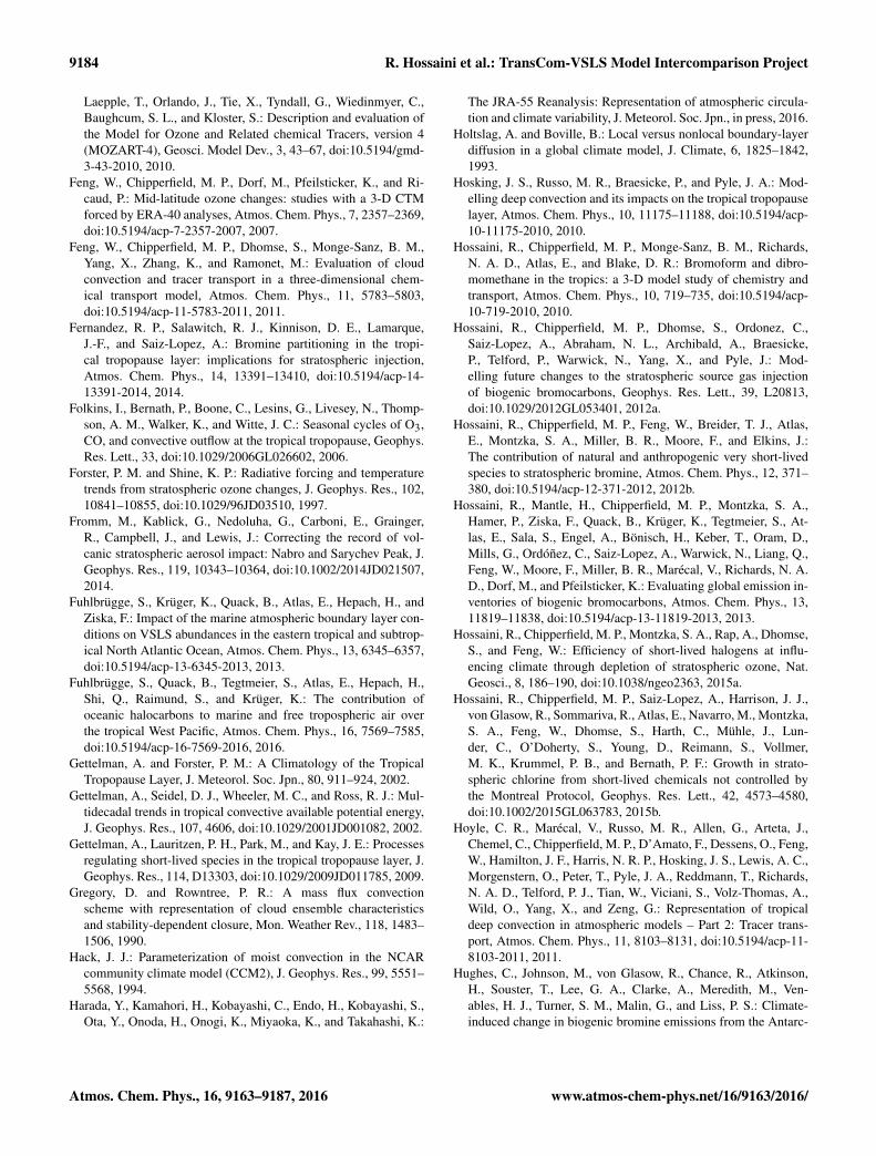
9184 R. Hossaini et al.: TransCom-VSLS Model Intercomparison Project
Laepple, T., Orlando, J., Tie, X., Tyndall, G., Wiedinmyer, C.,Baughcum, S. L., and Kloster, S.: Description and evaluation ofthe Model for Ozone and Related chemical Tracers, version 4(MOZART-4), Geosci. Model Dev., 3, 43–67, doi:10.5194/gmd-3-43-2010, 2010.
Feng, W., Chipperfield, M. P., Dorf, M., Pfeilsticker, K., and Ri-caud, P.: Mid-latitude ozone changes: studies with a 3-D CTMforced by ERA-40 analyses, Atmos. Chem. Phys., 7, 2357–2369,doi:10.5194/acp-7-2357-2007, 2007.
Feng, W., Chipperfield, M. P., Dhomse, S., Monge-Sanz, B. M.,Yang, X., Zhang, K., and Ramonet, M.: Evaluation of cloudconvection and tracer transport in a three-dimensional chem-ical transport model, Atmos. Chem. Phys., 11, 5783–5803,doi:10.5194/acp-11-5783-2011, 2011.
Fernandez, R. P., Salawitch, R. J., Kinnison, D. E., Lamarque,J.-F., and Saiz-Lopez, A.: Bromine partitioning in the tropi-cal tropopause layer: implications for stratospheric injection,Atmos. Chem. Phys., 14, 13391–13410, doi:10.5194/acp-14-13391-2014, 2014.
Folkins, I., Bernath, P., Boone, C., Lesins, G., Livesey, N., Thomp-son, A. M., Walker, K., and Witte, J. C.: Seasonal cycles of O3,CO, and convective outflow at the tropical tropopause, Geophys.Res. Lett., 33, doi:10.1029/2006GL026602, 2006.
Forster, P. M. and Shine, K. P.: Radiative forcing and temperaturetrends from stratospheric ozone changes, J. Geophys. Res., 102,10841–10855, doi:10.1029/96JD03510, 1997.
Fromm, M., Kablick, G., Nedoluha, G., Carboni, E., Grainger,R., Campbell, J., and Lewis, J.: Correcting the record of vol-canic stratospheric aerosol impact: Nabro and Sarychev Peak, J.Geophys. Res., 119, 10343–10364, doi:10.1002/2014JD021507,2014.
Fuhlbrügge, S., Krüger, K., Quack, B., Atlas, E., Hepach, H., andZiska, F.: Impact of the marine atmospheric boundary layer con-ditions on VSLS abundances in the eastern tropical and subtrop-ical North Atlantic Ocean, Atmos. Chem. Phys., 13, 6345–6357,doi:10.5194/acp-13-6345-2013, 2013.
Fuhlbrügge, S., Quack, B., Tegtmeier, S., Atlas, E., Hepach, H.,Shi, Q., Raimund, S., and Krüger, K.: The contribution ofoceanic halocarbons to marine and free tropospheric air overthe tropical West Pacific, Atmos. Chem. Phys., 16, 7569–7585,doi:10.5194/acp-16-7569-2016, 2016.
Gettelman, A. and Forster, P. M.: A Climatology of the TropicalTropopause Layer, J. Meteorol. Soc. Jpn., 80, 911–924, 2002.
Gettelman, A., Seidel, D. J., Wheeler, M. C., and Ross, R. J.: Mul-tidecadal trends in tropical convective available potential energy,J. Geophys. Res., 107, 4606, doi:10.1029/2001JD001082, 2002.
Gettelman, A., Lauritzen, P. H., Park, M., and Kay, J. E.: Processesregulating short-lived species in the tropical tropopause layer, J.Geophys. Res., 114, D13303, doi:10.1029/2009JD011785, 2009.
Gregory, D. and Rowntree, P. R.: A mass flux convectionscheme with representation of cloud ensemble characteristicsand stability-dependent closure, Mon. Weather Rev., 118, 1483–1506, 1990.
Hack, J. J.: Parameterization of moist convection in the NCARcommunity climate model (CCM2), J. Geophys. Res., 99, 5551–5568, 1994.
Harada, Y., Kamahori, H., Kobayashi, C., Endo, H., Kobayashi, S.,Ota, Y., Onoda, H., Onogi, K., Miyaoka, K., and Takahashi, K.:
The JRA-55 Reanalysis: Representation of atmospheric circula-tion and climate variability, J. Meteorol. Soc. Jpn., in press, 2016.
Holtslag, A. and Boville, B.: Local versus nonlocal boundary-layerdiffusion in a global climate model, J. Climate, 6, 1825–1842,1993.
Hosking, J. S., Russo, M. R., Braesicke, P., and Pyle, J. A.: Mod-elling deep convection and its impacts on the tropical tropopauselayer, Atmos. Chem. Phys., 10, 11175–11188, doi:10.5194/acp-10-11175-2010, 2010.
Hossaini, R., Chipperfield, M. P., Monge-Sanz, B. M., Richards,N. A. D., Atlas, E., and Blake, D. R.: Bromoform and dibro-momethane in the tropics: a 3-D model study of chemistry andtransport, Atmos. Chem. Phys., 10, 719–735, doi:10.5194/acp-10-719-2010, 2010.
Hossaini, R., Chipperfield, M. P., Dhomse, S., Ordonez, C.,Saiz-Lopez, A., Abraham, N. L., Archibald, A., Braesicke,P., Telford, P., Warwick, N., Yang, X., and Pyle, J.: Mod-elling future changes to the stratospheric source gas injectionof biogenic bromocarbons, Geophys. Res. Lett., 39, L20813,doi:10.1029/2012GL053401, 2012a.
Hossaini, R., Chipperfield, M. P., Feng, W., Breider, T. J., Atlas,E., Montzka, S. A., Miller, B. R., Moore, F., and Elkins, J.:The contribution of natural and anthropogenic very short-livedspecies to stratospheric bromine, Atmos. Chem. Phys., 12, 371–380, doi:10.5194/acp-12-371-2012, 2012b.
Hossaini, R., Mantle, H., Chipperfield, M. P., Montzka, S. A.,Hamer, P., Ziska, F., Quack, B., Krüger, K., Tegtmeier, S., At-las, E., Sala, S., Engel, A., Bönisch, H., Keber, T., Oram, D.,Mills, G., Ordóñez, C., Saiz-Lopez, A., Warwick, N., Liang, Q.,Feng, W., Moore, F., Miller, B. R., Marécal, V., Richards, N. A.D., Dorf, M., and Pfeilsticker, K.: Evaluating global emission in-ventories of biogenic bromocarbons, Atmos. Chem. Phys., 13,11819–11838, doi:10.5194/acp-13-11819-2013, 2013.
Hossaini, R., Chipperfield, M. P., Montzka, S. A., Rap, A., Dhomse,S., and Feng, W.: Efficiency of short-lived halogens at influ-encing climate through depletion of stratospheric ozone, Nat.Geosci., 8, 186–190, doi:10.1038/ngeo2363, 2015a.
Hossaini, R., Chipperfield, M. P., Saiz-Lopez, A., Harrison, J. J.,von Glasow, R., Sommariva, R., Atlas, E., Navarro, M., Montzka,S. A., Feng, W., Dhomse, S., Harth, C., Mühle, J., Lun-der, C., O’Doherty, S., Young, D., Reimann, S., Vollmer,M. K., Krummel, P. B., and Bernath, P. F.: Growth in strato-spheric chlorine from short-lived chemicals not controlled bythe Montreal Protocol, Geophys. Res. Lett., 42, 4573–4580,doi:10.1002/2015GL063783, 2015b.
Hoyle, C. R., Marécal, V., Russo, M. R., Allen, G., Arteta, J.,Chemel, C., Chipperfield, M. P., D’Amato, F., Dessens, O., Feng,W., Hamilton, J. F., Harris, N. R. P., Hosking, J. S., Lewis, A. C.,Morgenstern, O., Peter, T., Pyle, J. A., Reddmann, T., Richards,N. A. D., Telford, P. J., Tian, W., Viciani, S., Volz-Thomas, A.,Wild, O., Yang, X., and Zeng, G.: Representation of tropicaldeep convection in atmospheric models – Part 2: Tracer trans-port, Atmos. Chem. Phys., 11, 8103–8131, doi:10.5194/acp-11-8103-2011, 2011.
Hughes, C., Johnson, M., von Glasow, R., Chance, R., Atkinson,H., Souster, T., Lee, G. A., Clarke, A., Meredith, M., Ven-ables, H. J., Turner, S. M., Malin, G., and Liss, P. S.: Climate-induced change in biogenic bromine emissions from the Antarc-
Atmos. Chem. Phys., 16, 9163–9187, 2016 www.atmos-chem-phys.net/16/9163/2016/
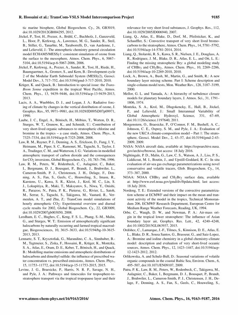
R. Hossaini et al.: TransCom-VSLS Model Intercomparison Project 9185
tic marine biosphere, Global Biogeochem. Cy., 26, GB3019,doi:10.1029/2012GB004295, 2012.
Jöckel, P., Tost, H., Pozzer, A., Brühl, C., Buchholz, J., Ganzeveld,L., Hoor, P., Kerkweg, A., Lawrence, M. G., Sander, R., Steil,B., Stiller, G., Tanarhte, M., Taraborrelli, D., van Aardenne, J.,and Lelieveld, J.: The atmospheric chemistry general circulationmodel ECHAM5/MESSy1: consistent simulation of ozone fromthe surface to the mesosphere, Atmos. Chem. Phys., 6, 5067–5104, doi:10.5194/acp-6-5067-2006, 2006.
Jöckel, P., Kerkweg, A., Pozzer, A., Sander, R., Tost, H., Riede, H.,Baumgaertner, A., Gromov, S., and Kern, B.: Development cycle2 of the Modular Earth Submodel System (MESSy2), Geosci.Model Dev., 3, 717–752, doi:10.5194/gmd-3-717-2010, 2010.
Krüger, K. and Quack, B.: Introduction to special issue: the Trans-Brom Sonne expedition in the tropical West Pacific, Atmos.Chem. Phys., 13, 9439–9446, doi:10.5194/acp-13-9439-2013,2013.
Lacis, A. A., Wuebbles, D. J., and Logan, J. A.: Radiative forc-ing of climate by changes in the vertical distribution of ozone, J.Geophys. Res., 95, 9971–9981, doi:10.1029/JD095iD07p09971,1990.
Laube, J. C., Engel, A., Bönisch, H., Möbius, T., Worton, D. R.,Sturges, W. T., Grunow, K., and Schmidt, U.: Contribution ofvery short-lived organic substances to stratospheric chlorine andbromine in the tropics – a case study, Atmos. Chem. Phys., 8,7325–7334, doi:10.5194/acp-8-7325-2008, 2008.
Law, R. M., Rayner, P. J., Denning, A. S., Erickson, D., Fung, I. Y.,Heimann, M., Piper, S. C., Ramonet, M., Taguchi, S., Taylor, J.A., Trudinger, C. M., and Watterson, I. G.: Variations in modelledatmospheric transport of carbon dioxide and the consequencesfor CO2 inversions, Global Biogeochem. Cy., 10, 783–796, 1996.
Law, R. M., Peters, W., Rödenbeck, C., Aulagnier, C., Baker,I., Bergmann, D. J., Bousquet, P., Brandt, J., Bruhwiler, L.,Cameron-Smith, P. J., Christensen, J. H., Delage, F., Den-ning, A. S., Fan, S., Geels, C., Houweling, S., Imasu, R.,Karstens, U., Kawa, S. R., Kleist, J., Krol, M. C., Lin, S.J., Lokupitiya, R., Maki, T., Maksyutov, S., Niwa, Y., Onishi,R., Parazoo, N., Patra, P. K., Pieterse, G., Rivier, L., Satoh,M., Serrar, S., Taguchi, S., Takigawa, M., Vautard, R., Ver-meulen, A. T., and Zhu, Z.: TransCom model simulations ofhourly atmospheric CO2: Experimental overview and diurnalcycle results for 2002, Global Biogeochem. Cy., 22, GB3009,doi:10.1029/2007gb003050, 2008.
Leedham, E. C., Hughes, C., Keng, F. S. L., Phang, S.-M., Malin,G., and Sturges, W. T.: Emission of atmospherically significanthalocarbons by naturally occurring and farmed tropical macroal-gae, Biogeosciences, 10, 3615–3633, doi:10.5194/bg-10-3615-2013, 2013.
Lennartz, S. T., Krysztofiak, G., Marandino, C. A., Sinnhuber, B.-M., Tegtmeier, S., Ziska, F., Hossaini, R., Krüger, K., Montzka,S. A., Atlas, E., Oram, D. E., Keber, T., Bönisch, H., and Quack,B.: Modelling marine emissions and atmospheric distributions ofhalocarbons and dimethyl sulfide: the influence of prescribed wa-ter concentration vs. prescribed emissions, Atmos. Chem. Phys.,15, 11753–11772, doi:10.5194/acp-15-11753-2015, 2015.
Levine, J. G., Braesicke, P., Harris, N. R. P., Savage, N. H.,and Pyle, J. A.: Pathways and timescales for troposphere-to-stratosphere transport via the tropical tropopause layer and their
relevance for very short lived substances, J. Geophys. Res., 112,doi:10.1029/2005JD006940, 2007.
Liang, Q., Atlas, E., Blake, D., Dorf, M., Pfeilsticker, K., andSchauffler, S.: Convective transport of very short lived bromo-carbons to the stratosphere, Atmos. Chem. Phys., 14, 5781–5792,doi:10.5194/acp-14-5781-2014, 2014.
Liang, Q., Stolarski, R. S., Kawa, S. R., Nielsen, J. E., Douglass, A.R., Rodriguez, J. M., Blake, D. R., Atlas, E. L., and Ott, L. E.:Finding the missing stratospheric Bry: a global modeling studyof CHBr3 and CH2Br2, Atmos. Chem. Phys., 10, 2269–2286,doi:10.5194/acp-10-2269-2010, 2010.
Lock, A., Brown, A., Bush, M., Martin, G., and Smith, R.: A newboundary layer mixing scheme. Part I: Scheme description andsingle-column model tests, Mon. Weather Rev., 128, 3187–3199,2000.
Mellor, G. L. and Yamada, A.: A hierarchy of turbulence closuremodels for planetary boundary layers, J. Atmos. Sci., 31, 1791–1806, 1974.
Montzka, S. A., Krol, M., Dlugokencky, E., Hall, B., Jöckel,P., and Lelieveld, J.: Small Interannual Variability ofGlobal Atmospheric Hydroxyl, Science, 331, 67–69,doi:10.1126/science.1197640, 2011.
Morgenstern, O., Braesicke, P., O’Connor, F. M., Bushell, A. C.,Johnson, C. E., Osprey, S. M., and Pyle, J. A.: Evaluation ofthe new UKCA climate-composition model – Part 1: The strato-sphere, Geosci. Model Dev., 2, 43–57, doi:10.5194/gmd-2-43-2009, 2009.
NASA: NASA aircraft data, available at: https://espoarchive.nasa.gov/archive/browse, last access: 18 July 2016.
Nightingale, P. D., Malin, G., Law, C. S., Watson, A. J., Liss, P. S.,Liddicoat, M. I., Boutin, J., and Upstill-Goddard, R. C.: In situevaluation of air-sea gas exchange parameterizations using novelconservative and volatile tracers, Glob. Biogeochem. Cy., 14,373–387, 2000.
NOAA: NOAA CHBr3 and CH2Br2 surface data, availableat: http://www.esrl.noaa.gov/gmd/dv/ftpdata.html, last access:18 July 2016.
Nordeng, T. E.: Extended versions of the convective parametriza-tion scheme at ECMWF and their impact on the mean and tran-sient activity of the model in the tropics, Technical Momoran-dum 206, ECMWF Research Department, European Centre forMedium Range Weather Forecasts, Reading, UK, 1994.
Orbe, C., Waugh, D. W., and Newman, P. A.: Air-mass ori-gin in the tropical lower stratosphere: The influence of Asianboundary layer air, Geophys. Res. Lett., 42, 4240–4248,doi:10.1002/2015GL063937, 2015.
Ordóñez, C., Lamarque, J.-F., Tilmes, S., Kinnison, D. E., Atlas, E.L., Blake, D. R., Sousa Santos, G., Brasseur, G., and Saiz-Lopez,A.: Bromine and iodine chemistry in a global chemistry-climatemodel: description and evaluation of very short-lived oceanicsources, Atmos. Chem. Phys., 12, 1423–1447, doi:10.5194/acp-12-1423-2012, 2012.
Orlikowska, A. and Schulz-Bull, D.: Seasonal variations of volatileorganic compounds in the coastal Baltic Sea, Environ. Chem., 6,495–507, doi:10.1071/EN09107, 2009.
Patra, P. K., Law, R. M., Peters, W., Rodenbeck, C., Takigawa, M.,Aulagnier, C., Baker, I., Bergmann, D. J., Bousquet, P., Brandt,J., Bruhwiler, L., Cameron-Smith, P. J., Christensen, J. H., De-lage, F., Denning, A. S., Fan, S., Geels, C., Houweling, S.,
www.atmos-chem-phys.net/16/9163/2016/ Atmos. Chem. Phys., 16, 9163–9187, 2016
9186 R. Hossaini et al.: TransCom-VSLS Model Intercomparison Project
Imasu, R., Karstens, U., Kawa, S. R., Kleist, J., Krol, M. C.,Lin, S.-J., Lokupitiya, R., Maki, T., Maksyutov, S., Niwa, Y.,Onishi, R., Parazoo, N., Pieterse, G., Rivier, L., Satoh, M., Ser-rar, S., Taguchi, S., Vautard, R., Vermeulen, A. T., and Zhu, Z.:TransCom model simulations of hourly atmospheric CO2: analy-sis of synoptic-scale variations for the period 2002–2003, GlobalBiogeochem. Cy., 22, GB4013, doi:10.1029/2007GB003081,2008.
Patra, P. K., Takigawa, M., Dutton, G. S., Uhse, K., Ishijima, K.,Lintner, B. R., Miyazaki, K., and Elkins, J. W.: Transport mech-anisms for synoptic, seasonal and interannual SF6 variations and“age” of air in troposphere, Atmos. Chem. Phys., 9, 1209–1225,doi:10.5194/acp-9-1209-2009, 2009.
Patra, P. K., Houweling, S., Krol, M., Bousquet, P., Belikov, D.,Bergmann, D., Bian, H., Cameron-Smith, P., Chipperfield, M. P.,Corbin, K., Fortems-Cheiney, A., Fraser, A., Gloor, E., Hess, P.,Ito, A., Kawa, S. R., Law, R. M., Loh, Z., Maksyutov, S., Meng,L., Palmer, P. I., Prinn, R. G., Rigby, M., Saito, R., and Wilson,C.: TransCom model simulations of CH4 and related species:linking transport, surface flux and chemical loss with CH4 vari-ability in the troposphere and lower stratosphere, Atmos. Chem.Phys., 11, 12813–12837, doi:10.5194/acp-11-12813-2011, 2011.
Pfeilsticker, K., Sturges, W. T., Bösch, H., Camy-Peyret, C., Chip-perfield, M. P., Engel, A., Fitzenberger, R., Müller, M., Payan,S., and Sinnhuber, B.-M.: Lower stratospheric organic and in-organic bromine budget for the Artic winter 1998/99, Geophys.Res. Lett., 27, 3305–3308, 2000.
Phang, S-M., Keng, FS-L., Paramjeet-Kaur, M. S., Lim, Y-K., Rah-man, N. A., Leedham, E. C., Robinson, A. D., Harris, N. R. P.,Pyle, J. A., and Sturges, W. T.: Can seaweed farming in the trop-ics contribute to climate change through emissions of short-livedhalocarbons, Malaysian Journal of Science, 34, 8–19, 2015.
Pisso, I., Haynes, P. H., and Law, K. S.: Emission loca-tion dependent ozone depletion potentials for very short-livedhalogenated species, Atmos. Chem. Phys., 10, 12025–12036,doi:10.5194/acp-10-12025-2010, 2010.
Pyle, J. A., Ashfold, M. J., Harris, N. R. P., Robinson, A. D., War-wick, N. J., Carver, G. D., Gostlow, B., O’Brien, L. M., Manning,A. J., Phang, S. M., Yong, S. E., Leong, K. P., Ung, E. H., andOng, S.: Bromoform in the tropical boundary layer of the Mar-itime Continent during OP3, Atmos. Chem. Phys., 11, 529–542,doi:10.5194/acp-11-529-2011, 2011.
Quack, B. and Wallace, D.: Air-sea flux of bromoform: Con-trols, rates, and implications, Global Biogeochem. Cy., 17, 1023,doi:10.1029/2002GB001890, 2003.
Randel, W. J., Park, M., Emmons, L., Kinnison, D., Bernath, P.,Walker, K. A., Boone, C., and Pumphrey, H.: Asian MonsoonTransport of Pollution to the Stratosphere, Science, 328, 611–613, doi:10.1126/science.1182274, 2010.
Riese, M., Ploeger, F., Rap, A., Vogel, B., Konopka, P., Dameris, M.,and Forster, P.: Impact of uncertainties in atmospheric mixingon simulated UTLS composition and related radiative effects, J.Geophys. Res., 117, D16305, doi:10.1029/2012JD017751, 2012.
Robinson, A. D., Harris, N. R. P., Ashfold, M. J., Gostlow, B., War-wick, N. J., O’Brien, L. M., Beardmore, E. J., Nadzir, M. S.M., Phang, S. M., Samah, A. A., Ong, S., Ung, H. E., Peng,L. K., Yong, S. E., Mohamad, M., and Pyle, J. A.: Long-termhalocarbon observations from a coastal and an inland site in
Sabah, Malaysian Borneo, Atmos. Chem. Phys., 14, 8369–8388,doi:10.5194/acp-14-8369-2014, 2014.
Roeckner, E., Brokopf, R., Esch, M., Giorgetta, M., Hagemann, S.,Kornblueh, L., Manzini, E., Schlese, U., and Schulzweida, U.:Sensitivity of simulated climate to horizontal and vertical reso-lution in the ECHAM5 atmosphere model, J. Climate, 19, 3771–3791, doi:10.1175/JCLI3824.1, 2006.
Russo, M. R., Ashfold, M. J., Harris, N. R. P., and Pyle, J. A.: On theemissions and transport of bromoform: sensitivity to model res-olution and emission location, Atmos. Chem. Phys., 15, 14031–14040, doi:10.5194/acp-15-14031-2015, 2015.
Rybka, H. and Tost, H.: Uncertainties in future climate predictionsdue to convection parameterisations, Atmos. Chem. Phys., 14,5561–5576, doi:10.5194/acp-14-5561-2014, 2014.
Sala, S., Bönisch, H., Keber, T., Oram, D. E., Mills, G., andEngel, A.: Deriving an atmospheric budget of total organicbromine using airborne in situ measurements from the westernPacific area during SHIVA, Atmos. Chem. Phys., 14, 6903–6923,doi:10.5194/acp-14-6903-2014, 2014.
Salawitch, R., Weisenstein, D., Kovalenko, L., Sioris, C.,Wennberg, P., Chance, K., Ko, M., and McLinden, C.: Sensitiv-ity of ozone to bromine in the lower stratosphere, Geophys. Res.Lett., 32, L05811, doi:10.1029/2004GL021504, 2005.
Sander, S., Friedl, R., Barker, J., Golden, D., Kurylo, M., Wine, P.,Abbatt, J., Burkholder, J., Kolb, C., Moortgat, G., Huie, R., andOrkin, V.: Chemical Kinetics and Photochemical Data for Usein Atmospheric Studies, Evaluation Number 17, JPL Publication10-6, Jet Propulsion Laboratory, 2011.
Sinnhuber, B.-M. and Meul, S.: Simulating the impact of emis-sions of brominated very short lived substances on past strato-spheric ozone trends, Geophys. Res. Lett., 42, 2449–2456,doi:10.1002/2014GL062975, 2015.
Sinnhuber, B.-M., Sheode, N., Sinnhuber, M., Chipperfield, M. P.,and Feng, W.: The contribution of anthropogenic bromine emis-sions to past stratospheric ozone trends: a modelling study, At-mos. Chem. Phys., 9, 2863–2871, doi:10.5194/acp-9-2863-2009,2009.
Stemmler, I., Hense, I., and Quack, B.: Marine sources of bromo-form in the global open ocean – global patterns and emissions,Biogeosciences, 12, 1967–1981, doi:10.5194/bg-12-1967-2015,2015.
Sturges, W., Oram, D., Carpenter, L., Penkett, S., and Engel, A.:Bromoform as a source of stratospheric bromine, Geophys. Res.Lett., 27, 2081–2084, doi:10.1029/2000GL011444, 2000.
Taguchi, S.: A three-dimensional model of atmospheric CO2 trans-port based on analyzed winds: Model description and simulationresults for TRANSCOM, J. Geophys Res., 101, 15099–15109,doi:10.1029/96JD00504, 1996.
Taguchi, S., Tasaka, S., Matsubara, M., Osada, K., Yokoi, T., andYamanouchi, T.: Air-sea gas transfer rate for the Southern Oceaninferred from 222Rn concentrations in maritime air and a globalatmospheric transport model, J. Geophys. Res., 118, 7606–7616,doi:10.1002/jgrd.50594, 2013.
Tegtmeier, S., Krüger, K., Quack, B., Atlas, E. L., Pisso, I., Stohl,A., and Yang, X.: Emission and transport of bromocarbons:from the West Pacific ocean into the stratosphere, Atmos. Chem.Phys., 12, 10633–10648, doi:10.5194/acp-12-10633-2012, 2012.
Tegtmeier, S., Krüger, K., Quack, B., Atlas, E., Blake, D. R.,Boenisch, H., Engel, A., Hepach, H., Hossaini, R., Navarro, M.
Atmos. Chem. Phys., 16, 9163–9187, 2016 www.atmos-chem-phys.net/16/9163/2016/
R. Hossaini et al.: TransCom-VSLS Model Intercomparison Project 9187
A., Raimund, S., Sala, S., Shi, Q., and Ziska, F.: The contributionof oceanic methyl iodide to stratospheric iodine, Atmos. Chem.Phys., 13, 11869–11886, doi:10.5194/acp-13-11869-2013, 2013.
Tegtmeier, S., Ziska, F., Pisso, I., Quack, B., Velders, G. J. M., Yang,X., and Krüger, K.: Oceanic bromoform emissions weighted bytheir ozone depletion potential, Atmos. Chem. Phys., 15, 13647–13663, doi:10.5194/acp-15-13647-2015, 2015.
Thompson, R. L., Patra, P. K., Ishijima, K., Saikawa, E., Corazza,M., Karstens, U., Wilson, C., Bergamaschi, P., Dlugokencky, E.,Sweeney, C., Prinn, R. G., Weiss, R. F., O’Doherty, S., Fraser,P. J., Steele, L. P., Krummel, P. B., Saunois, M., Chipperfield,M., and Bousquet, P.: TransCom N2O model inter-comparison– Part 1: Assessing the influence of transport and surface fluxeson tropospheric N2O variability, Atmos. Chem. Phys., 14, 4349–4368, doi:10.5194/acp-14-4349-2014, 2014.
Tiedtke, M.: A comprehensive mass flux scheme for cu-mulus parameterization in large-scale models, Mon.Weather Rev., 117, 1779–1800, doi:10.1175/1520-0493(1989)117<1779:ACMFSF>2.0.CO;2, 1989.
Tilmes, S., Kinnison, D. E., Garcia, R. R., Salawitch, R., Canty, T.,Lee-Taylor, J., Madronich, S., and Chance, K.: Impact of veryshort-lived halogens on stratospheric ozone abundance and UVradiation in a geo-engineered atmosphere, Atmos. Chem. Phys.,12, 10945–10955, doi:10.5194/acp-12-10945-2012, 2012.
Tissier, A.-S. and Legras, B.: Convective sources of trajectoriestraversing the tropical tropopause layer, Atmos. Chem. Phys., 16,3383–3398, doi:10.5194/acp-16-3383-2016, 2016.
Vogel, B., Günther, G., Müller, R., Grooß, J.-U., Hoor, P., Krämer,M., Müller, S., Zahn, A., and Riese, M.: Fast transport fromSoutheast Asia boundary layer sources to northern Europe: rapiduplift in typhoons and eastward eddy shedding of the Asianmonsoon anticyclone, Atmos. Chem. Phys., 14, 12745–12762,doi:10.5194/acp-14-12745-2014, 2014.
Warwick, N. J., Pyle, J. A., Carver, G. D., Yang, X., Savage,N. H., O’Connor, F. M., and Cox, R. A.: Global modelingof biogenic bromocarbons, J. Geophys. Res., 111, D24305,doi:10.1029/2006JD007264, 2006.
Werner, B., Atlas, E., Cheung, R., Chipperfield, M. P., Colosimo, F.,Daube, B., Deutschmann, T., Elkins, J. W., Fahey, D. W., Feng,W., Festa, J., Gao, R-S., Hintsa, E. J., Hossaini, R., Moore, F. L.,Navarro, M. A., Pittman, J., Raecke, R., Scalone, L., Spolaor, M.,Stutz, J., Thornberry, T. D., Tsai, C., Wofsy, S., and Pfeilsticker,K.: Probing the subtropical lowermost stratosphere, tropical up-per troposphere, and tropopause layer for inorganic bromine, At-mos. Chem. Phys. Discuss., in preparation, 2016.
Wisher, A., Oram, D. E., Laube, J. C., Mills, G. P., van Velthoven,P., Zahn, A., and Brenninkmeijer, C. A. M.: Very short-lived bro-momethanes measured by the CARIBIC observatory over theNorth Atlantic, Africa and Southeast Asia during 2009–2013,Atmos. Chem. Phys., 14, 3557–3570, doi:10.5194/acp-14-3557-2014, 2014.
WMO: Scientific Assessment of Ozone Depletion: 2014, GlobalOzone Research and Monitoring Project, Report No. 55, WorldMeteorological Organization, Geneva, Switzerland, 2014.
Wofsy, S. C., Team, H. S., Team, C. M., and Team, S.: HIA-PER Pole-to-Pole Observations (HIPPO): fine-grained, global-scale measurements of climatically important atmosphericgases and aerosols, Philos. T. R. Soc., 369, 2073–2086,doi:10.1098/rsta.2010.0313, 2011.
Wofsy, S. C., Daube, B. C., Jimenez, R., Kort, E., Pittman, J.V., Park, S., Commane, R., Xiang, B., Santoni, G., Jacob, D.,Fisher, J., Pickett-Heaps, C., Wang, H., Wecht, K., Wang, Q.-Q.,Stephens, B. B., Shertz, S., Watt, A. S., Romashkin, P., Cam-pos, T., Haggerty, J., Cooper, W. A., Rogers, D., Beaton, S., Hen-dershot, R., Elkins, J. W., Fahey, D. W., Gao, R. S., Moore, F.,Montzka, S. A., Schwarz, J. P., Perring, A. E., Hurst, D., Miller,B. R., Sweeney, C., Oltmans, S., Nance, D., Hintsa, E., Dut-ton, G., Watts, L. A., Spackman, J. R., Rosenlof, K. H., Ray,E. A., Hall, B., Zondlo, M. A., Diao, M., Keeling, R., Bent,J., Atlas, E. L., Lueb, R., and Mahoney, M. J.: HIPPO aircraftdata, HIPPO Combined Discrete Flask and GC Sample GHG,Halo-, Hydrocarbon Data (R_20121129), Carbon Dioxide Infor-mation Analysis Center, Oak Ridge National Laboratory, OakRidge, Tennessee, USA, doi:10.3334/CDIAC/hippo_012 (Re-lease 20121129), last access: 18 July 2016.
Wolter, K. and Timlin, M. S.: Measuring the strength of ENSOevents: How does 1997/98 rank?, Weather, 53, 315–324,doi:10.1002/j.1477-8696.1998.tb06408.x, 1998.
Yang, X., Abraham, N. L., Archibald, A. T., Braesicke, P., Keeble,J., Telford, P. J., Warwick, N. J., and Pyle, J. A.: How sensitiveis the recovery of stratospheric ozone to changes in concentra-tions of very short-lived bromocarbons?, Atmos. Chem. Phys.,14, 10431–10438, doi:10.5194/acp-14-10431-2014, 2014.
Zhang, K., Wan, H., Zhang, M., and Wang, B.: Evaluation of the at-mospheric transport in a GCM using radon measurements: sen-sitivity to cumulus convection parameterization, Atmos. Chem.Phys., 8, 2811–2832, doi:10.5194/acp-8-2811-2008, 2008.
Zhang, G. J. and McFarlane, N. A.: Sensitivity of climate simula-tions to the parameterization of cumulus convection in the Cana-dian climate centre general circulation model, Atmos. Ocean, 33,407–446, 1995.
Ziska, F., Quack, B., Abrahamsson, K., Archer, S. D., Atlas, E.,Bell, T., Butler, J. H., Carpenter, L. J., Jones, C. E., Harris, N. R.P., Hepach, H., Heumann, K. G., Hughes, C., Kuss, J., Krüger,K., Liss, P., Moore, R. M., Orlikowska, A., Raimund, S., Reeves,C. E., Reifenhäuser, W., Robinson, A. D., Schall, C., Tanhua,T., Tegtmeier, S., Turner, S., Wang, L., Wallace, D., Williams, J.,Yamamoto, H., Yvon-Lewis, S., and Yokouchi, Y.: Global sea-to-air flux climatology for bromoform, dibromomethane and methyliodide, Atmos. Chem. Phys., 13, 8915–8934, doi:10.5194/acp-13-8915-2013, 2013.
www.atmos-chem-phys.net/16/9163/2016/ Atmos. Chem. Phys., 16, 9163–9187, 2016