a multi-objective chance-constrained programming …
TRANSCRIPT

water
Article
A Multi-Objective Chance-Constrained ProgrammingApproach for Uncertainty-Based Optimal NutrientsLoad Reduction at the Watershed Scale
Xujun Liu 1, Mengjiao Zhang 2, Han Su 2, Feifei Dong 2, Yao Ji 2,3,* and Yong Liu 2,3
1 College of Environment Science and Engineering, Tongji University, Shanghai 20092, China;[email protected]
2 College of Environmental Science and Engineering, Key Laboratory of Water and Sediment Sciences (MOE),Peking University, Beijing 100871, China; [email protected] (M.Z.); [email protected] (H.S.);[email protected] (F.D.); [email protected] (Y.L.)
3 Yunnan Key Laboratory of Pollution Process and Management of Plateau Lake-Watershed,Kunming 650034, China
* Correspondence: [email protected]; Tel.: +86-10-6275-3184
Academic Editor: Gordon HuangReceived: 1 March 2017; Accepted: 27 April 2017; Published: 3 May 2017
Abstract: A multi-objective chance-constrained programming integrated with Genetic Algorithmand robustness evaluation methods was proposed to weigh the conflict between system investmentagainst risk for watershed load reduction, which was firstly applied to nutrient load reduction in theLake Qilu watershed of the Yunnan Plateau, China. Eight sets of Pareto solutions were acceptable forboth system investment and probability of constraint satisfaction, which were selected from 23 setsof Pareto solutions out of 120 solution sets. Decision-makers can select optimal decisions from thesolutions above in accordance with the actual conditions of different sub-watersheds under variousengineering measures. The relationship between system investment and risk demonstrated thatsystem investment increased rapidly when the probability level of constraint satisfaction was higherthan 0.9, but it reduced significantly if appropriate risk was permitted. Evaluation of robustness of theoptimal scheme indicated that the Pareto solution obtained from the model provided the ideal option,since the solutions were always on the Pareto frontier under various distributions and mean valuesof the random parameters. The application of the multi-objective chance-constrained programmingto optimize the reduction of watershed nutrient loads in Lake Qilu indicated that it is also applicableto other environmental problems or study areas that contain uncertainties.
Keywords: multi-objective chance-constrained programming; genetic algorithm; robustnessevaluation; watershed load reduction; Lake Qilu
1. Introduction
Lake eutrophication is one of the greatest environmental challenges, which hampers and destroysecological functions of water bodies, and leads to deterioration of water quality [1,2]. Many irreversibleeffects on aquatic ecosystems and drinking water supplies have resulted from degeneration ofwater quality, and this issue has become the principal bottleneck to the sustainable developmentof watersheds and the protection of human health [3–5]. Watershed planning and management ofwater quality is imperative. Load reduction of watershed nutrients (mainly Nitrogen and Phosphorus)is an effective approach to water quality improvement. Load reduction is also an important approachto balancing watershed development and protection of water quality, because nutrient loads to waterbodies are mainly due to human production and activities, and they are a primary cause of waterquality impairment [6,7]. Optimization models are applied widely to provide effective load reduction
Water 2017, 9, 322; doi:10.3390/w9050322 www.mdpi.com/journal/water

Water 2017, 9, 322 2 of 18
schemes as a technical basis for watershed management [8–10]. Optimization models for watershedload reduction provide pollution control schemes that can produce efficient management of watershedload reductions under the constraint of watershed development and human demands.
A multitude of programming methods have been proposed to deal with load reduction forprotection of water quality [11–13]. Among these, much research has focused on representing anddealing with uncertainties, because uncertainties in the components and related impact factors withinthe system cause optimization problems to be more complicated [14,15]. On the other hand, studies onmulti-objective models continuously spring up, because taking the diverse demands of social economicprogress and environmental protection into account it is necessary, and using multi-objective modelscan balance the conflict between different optimal objectives, such as economic development andrestoration of water quality [16–19]. Uncertainty in the system also resulted from some influencefactors having random characteristics, which originates from natural processes in the hydrologicalcycle, and variation in water pollution over time and space [20–22]. That is to say, uncertainty andmulti-objective problems should be considered simultaneously, however, few studies have beenconducted on optimization of load reduction in watersheds while considering both uncertainty andthe weighting of multiple objectives. Not considering the balancing of multiple objectives or thehandling of uncertainty results in a shortage of information in the optimization process, and schemesthat are based on inapposite fundamental assumptions will lack the capacity both to reflect on practicalsituations and to provide a planning scheme for decision-makers. Thus, a multi-objective programmingmethod that accounts for uncertainty in reducing pollution loads to improve water quality is imperativeand practical.
In this study, a multi-objective chance-constrained programming integrated with GeneticAlgorithm (GA) and robustness evaluation methods was proposed to optimize load reduction ofnutrients in the Lake Qilu watershed. The objective function was composed of minimal systemcosts and maximization of water qualification rate. Typical impact factors (Total Nitrogen and TotalPhosphorus, TN and TP) were incorporated, and the primary pollution sources, such as agriculturalnon-point pollution, urban non-point pollution, and livestock pollution, were included. From this,constraints in the optimal model were selected, such as reduction of TN and TP from agriculturalnon-point pollution, domestic sewage treatment level, municipal solid waste disposal, and ecologicalrestoration. Optimization schemes were obtained to find the tradeoff between system investment andrisk, and estimation of the model’s robustness was conducted.
2. Materials and Methods
2.1. Study Area
Lake Qilu is one of the nine plateau lakes in Yunnan Province, China, and it is also the naturalfoundation for development of Tonghai Country, Yuxi City, which has been seriously contaminatedthrough natural processes and human activity in recent years. TN and TP are important indicators ofeutrophication for Lake Qilu, and nonpoint-source pollution from agricultural systems and livestockbreeding are the primary sources of pollution. TN from agricultural non-point source pollution (NPS)and livestock breeding are 33.04% and 37.56%, respectively, and TP from agricultural, nonpoint-sourcepollution and livestock breeding are 19.80% and 61.68%, respectively. In addition, household wasteis another major component of non-point source pollution, which contributes 23.17% and 14.70% toTN and TP, respectively. Thus, measures to reduce nutrient loads are necessary to control watershedpollution in the Lake Qilu watershed [23].
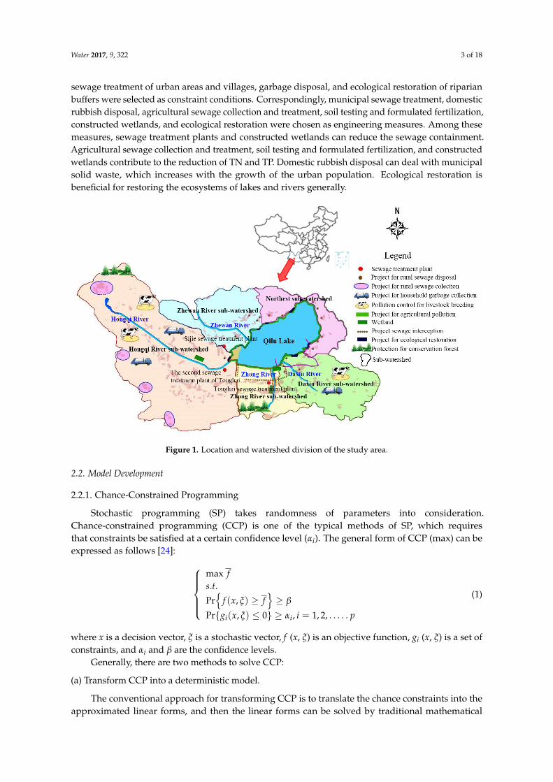
The Lake Qilu watershed contains five sub-watersheds, the Hongqi River sub-watershed, theZhewan River sub-watershed, the Zhong River sub-watershed, the Daxin River sub-watershed,and the Northest sub-watershed, which are selected as basic units for optimizing load reductions(Figure 1). According to watershed management requirements, “The 12th Five-Year Plan”, andpollution characteristics of Lake Qilu, reduction in TN and TP from agricultural, non-point pollution,
Water 2017, 9, 322 3 of 18
sewage treatment of urban areas and villages, garbage disposal, and ecological restoration of riparianbuffers were selected as constraint conditions. Correspondingly, municipal sewage treatment, domesticrubbish disposal, agricultural sewage collection and treatment, soil testing and formulated fertilization,constructed wetlands, and ecological restoration were chosen as engineering measures. Among thesemeasures, sewage treatment plants and constructed wetlands can reduce the sewage containment.Agricultural sewage collection and treatment, soil testing and formulated fertilization, and constructedwetlands contribute to the reduction of TN and TP. Domestic rubbish disposal can deal with municipalsolid waste, which increases with the growth of the urban population. Ecological restoration isbeneficial for restoring the ecosystems of lakes and rivers generally.
Water 2017, 9, 322 3 of 17
treatment of urban areas and villages, garbage disposal, and ecological restoration of riparian buffers were selected as constraint conditions. Correspondingly, municipal sewage treatment, domestic rubbish disposal, agricultural sewage collection and treatment, soil testing and formulated fertilization, constructed wetlands, and ecological restoration were chosen as engineering measures. Among these measures, sewage treatment plants and constructed wetlands can reduce the sewage containment. Agricultural sewage collection and treatment, soil testing and formulated fertilization, and constructed wetlands contribute to the reduction of TN and TP. Domestic rubbish disposal can deal with municipal solid waste, which increases with the growth of the urban population. Ecological restoration is beneficial for restoring the ecosystems of lakes and rivers generally.
Figure 1. Location and watershed division of the study area.
2.2. Model Development
2.2.1. Chance-Constrained Programming
Stochastic programming (SP) takes randomness of parameters into consideration. Chance-constrained programming (CCP) is one of the typical methods of SP, which requires that constraints be satisfied at a certain confidence level (αi). The general form of CCP (max) can be expressed as follows [24]:
{ }{ }
max. .
Pr ( , )
Pr ( , ) 0 , 1,2,.....i i
f
s t
f x f
g x i p
ξ β
ξ α
≥ ≥ ≤ ≥ =
(1)
where x is a decision vector, ξ is a stochastic vector, f (x, ξ) is an objective function, gi (x, ξ) is a set of constraints, and αi and β are the confidence levels.
Generally, there are two methods to solve CCP:
(a) Transform CCP into a deterministic model.
The conventional approach for transforming CCP is to translate the chance constraints into the approximated linear forms, and then the linear forms can be solved by traditional mathematical
Figure 1. Location and watershed division of the study area.
2.2. Model Development
2.2.1. Chance-Constrained Programming
Stochastic programming (SP) takes randomness of parameters into consideration.Chance-constrained programming (CCP) is one of the typical methods of SP, which requiresthat constraints be satisfied at a certain confidence level (αi). The general form of CCP (max) can beexpressed as follows [24]:
max fs.t.Pr{
f (x, ξ) ≥ f}≥ β
Pr{gi(x, ξ) ≤ 0} ≥ αi, i = 1, 2, . . . . . p
(1)
where x is a decision vector, ξ is a stochastic vector, f (x, ξ) is an objective function, gi (x, ξ) is a set ofconstraints, and αi and β are the confidence levels.
Generally, there are two methods to solve CCP:
(a) Transform CCP into a deterministic model.
The conventional approach for transforming CCP is to translate the chance constraints into theapproximated linear forms, and then the linear forms can be solved by traditional mathematical
Water 2017, 9, 322 4 of 18
models [25–27]. For objective functions in linear form and some specific nonlinear functions in whichparameters follow a normal distribution or an exponential distribution, approximated linear forms canbe obtained, and CCP can be transformed into its relevant deterministic programming [28,29].
(b) Stochastic simulation.
Stochastic simulation (i.e., Monte Carlo Simulation) is used widely in handling stochasticprogramming [30]. According to the fundamentals of Monte Carlo Simulation, the probability ofan event can be estimated by frequency that is gained from numerous tests, and the frequency isprobability when the sample size is large enough. For CCP:
Pr{gi(x, ξ) ≤ 0} ≥ α, i = 1, 2, ...p (2)
where ξ is a stochastic vector, and the cumulative probability distribution is Φ (ξ). If we set independentrandom variables (ξ1, ξ2, . . . , ξN) that are acquired from Φ (ξ) in N experiments, then N′ is the numberof times that the following formula holds:
gi(x, ξ j) ≤ 0, i = 1, 2, ..., p j = 1, 2, ..., N (3)
N′ is the number of random variables that satisfy constraints, and probability can be estimated byN′/N. Thus, CCP holds when N′/N ≥ α.
2.2.2. Multi-Objective Programming
The expression of multi-objective programming (MOP) is as follows [31]:{minF(x) =
{f1(x), f2(x), f3(x), ..., fq(x)
}s.t. gi(x) ≤ 0, i = 1, 2, 3, ..., m
(4)
Generally, a tradeoff among sub-objects in MOP is necessary to achieve an overall optimizationunder the conflict of the sub-objectives. The essential difference between MOP and single objectoptimization is that the optimization solution is not exclusive. The solution set of MOP is composed ofa series of Pareto optimal solutions.
The conventional approach for solving MOP is to convert the multi-objective problem to asingle-objective problem. Typically, this includes the constraint method, the weighting method, andthe distance function method [32]. Constraint method converts MOP to a SOP through transferringsecondary objectives to constraints that obey a certain requirement. Weighting method establishes anew objective function with original sub-objectives and the weight corresponding with them. Distancefunction method can search optimal solution that have the shortest distance for each sub-objectivein solutions space. Traditional methods inherit the mechanism of single objective optimization, butlimitations are obvious at the same time. First, the conventional approach, such as the weightingmethod, is too sensitive to the optimal frontier of a Pareto solution, and it is strongly subjective withrespect to weighted value distributions. Second, traditional methods obtain one solution at a time,thus, they require an enormous amount of time, and it is difficult to obtain an effective decision [33].
2.2.3. Genetic Algorithm
Genetic Algorithm (GA) is a global searching and optimization method developed fromsimulations of the natural evolutionary process that is based on Darwin’s theory of evolution andMendel’s theory of heredity. GA has been used widely in dealing with MOP due to its advantage ofbeing able to handle a large search space and for obtaining a series of Pareto optimal solutions at onetime. The basic process of GA is as follows [34]:
Water 2017, 9, 322 5 of 18
(a) Generate an initial population under some coding scheme;(b) Convert the encoded individuals to decision variables under the corresponding decoding method,
and calculate the adaptive value;(c) Set up a mating pool by selecting larger individuals from the population;(d) Develop a new generation after crossover and mutation;(e) Repeat steps 2–4 until the convergence criterion is satisfied.
GA is an efficient algorithm for solving the MOP problem, because it is possible to get multiple,optimal solutions and to acquire an optimal solution set at the same time. A series of newalgorithms has been developed from GA, such as Vector Evaluated Genetic Algorithm (VEGA),Multi-Objective Genetic Algorithm (MOGA), Non-dominated Sorting Genetic Algorithm (NSGA),and so on [35,36]. VEGA divides the population into M subpopulations and conduct SOP foreach subpopulation, and then repeat the process “population partition—optimization searchingfor each subpopulation—exchange of information between generations” until the optimal solutionsare obtained. Although VEGA is convenient in operation, it has the apparent defect that the optimalsolutions are generally the extreme points on the Pareto frontier and the Pareto solutions betweenthe extreme points are unable to get. MOGA seeks optimal solution by calculating fitness for eachindividual, which introduces a fitness-sharing model to apply different types of optimization problems.The deficiency of MOGA is that, if the selection in the Pareto solution is biased resulted from the fitnessvalue, the shape of Pareto frontier will be sensitive to spatial distribution of the solutions. NSGAproposes a hierarchical algorithm for Pareto solution searching, which guarantees the diversity ofsolution space and the homogeneity of Pareto frontier.
In this study, we selected CE-NSGA-II and applied it to the optimization problem to reducenutrient loads in a watershed. This algorithm has the advantage on large coverage of the solution setand a fast convergence rate, and has the ability to increase the population diversity under lower fitnessvalue [37].
2.2.4. Robustness of Decision Scheme
Decades of practical experience indicate that not all the information can be described and modeledwell by the tools of probability and statistics, and the tools of statistics modeling and analysis mayfail to express and handle precisely and properly the uncertainties that are posed by a complexsystem. The phenomenon above is called “deep uncertainty” [38–40]. Under deep uncertainty,robust decision-making was proposed to provide policies that are robust across multiple scenarios, oralternative models at low cost [41]. Robust decision-making gives priority to robustness of the decisionscheme rather than priority to optimization; that is to say, the decision scheme, which is insensitive touncertainty parameters, will still exhibit good performance under a changing scenario.
Robustness can be expressed as system adaptability:
Λ(d, X) =
{1 , Y(d, X) ≤ YT
0 , Y(d, X) > YT(5)
where Λ (d, X) is adaptation function, d is decision scheme, YT is threshold value, and X isdeep uncertainty.
In this study, estimating parameter RI is selected to assess robustness of the decision scheme,which is based on the hypothesis that every scenario happens with the same probability. Parametersettings of TN reduction of measure j (ANRj) and TP reduction of measure j (APRj) based on the abovetheory can be expressed as follows:
RI(d) =t
Λ(d, X)dx1dx2dx3tdx1dx2dx3
(6)

Water 2017, 9, 322 6 of 18
ANRj = µANRj ± 3σANRj (7)
APRj = µAPRj ± 3σAPRj (8)
2.3. Multi-Objective Stochastic Programming Model for Load Reduction in the Lake Qilu Watershed
2.3.1. Modeling Optimal Load Reduction
We developed an optimal model that used the Lake Qilu watershed as the management objective.We selected reduction of TN, TP, domestic sewage treatment and municipal solid waste; and ecologicalrestoration and the probability of constraint satisfaction as constraint conditions. Among them,reduction of TN and TP were selected as uncertain factors in terms of random parameters, sincethe pollution load of TN and TP show an obvious random feature depending on season [42,43].We also set the maximization of constraint satisfaction probability and the minimization of systemcost on load reduction as optimization objectives. Therefore, measures to reduce the costs of loadreduction included the cost of reducing TN and TP from agricultural non-point pollution, the cost ofsewage treatment for urban areas and villages, the cost of garbage disposal, and the cost of ecologicalrestoration of riparian buffers. The expression of the multi-objective, stochastic programming model isas follows.
(1) Objective functions.
(a) Minimize system cost:
min Fv =I
∑i=1
J
∑j=1
ASCi,j · Xi,j · ai,j (9)
(b) Maximize water qualification rate:
max Fp = Pr{UCm : ∀m = 1, 2}
= Pr
5∑
j=3ANRj · Xi,j · ai,j/TNDi ≥ RNDi
5∑
j=3APRj · Xi,j · ai,j/TPDi ≥ RPDi
(10)
In objective (b), UCm refers to the constraints containing randomness parameters (ANR and APR).
(2) Constraint conditions.
(a) TN from non-point source pollution in agricultural system:
UC1 :5
∑j=3
ANRj · Xi,j · ai,j/TNDi ≥ RNDi (11)
Reduction of TN from agricultural production (j = 3), rural domestic pollution (j = 4) andconstructed wetland (j = 5) should meet the requirements of non-point, source pollution (NPS) control.
(b) TP from non-point source pollution in agricultural system:
UC2 :5
∑j=3
APRj · Xi,j · ai,j/TPDi ≥ RPDi (12)
Reduction of TP from agricultural production (j = 3), rural domestic pollution (j = 4) andconstructed wetland (j = 5) should meet the requirements of non-point source pollution control.

Water 2017, 9, 322 7 of 18
(c) Domestic sewage:
(Xi,1ai,1 + Xi,3ai,3 + Xi,5 · ai,5 · K)/TWDi ≥ RWDi (13)
Domestic sewage treatment level should meet sewage treatment requirements, and engineeringmeasures related to domestic sewage is municipal wastewater treatment (j = 1), agricultural sewagecollection and treatment (j = 3), and constructed wetland (j = 5).
(d) Municipal solid waste:Xi,2 · ai,2/TRWi ≥ RRWi (14)
The level of municipal solid waste disposal should meet the relevant planning requirements.
(e) Ecological restoration:Xi,6 · ai,6 ≥ RFLi (15)
The ecological restoration constraint refers to the percentage of ecological restoration that satisfiesthe relevant planning requirements.
(f) Technical constraint:X±i,j ≥ 0 (16)
Reduction of TN and TP may include random effects that are affected by many uncertaintyelements, thus, it is necessary to quantify the random information effectively to obtain precise andproper schemes for decision-making. Assume that reduction of TN and TP obeys a normal distribution,where the mean value is µ and standard variation is σ. µ is obtained from the Manual of EngineeringMeasure Design, and σ is set as σ = µ × 10% (shown in Table 1). The constraint for CCP can beexpressed as follows:
Pr{gi(x, ξ) ≤ 0} ≥ αi, i = 1, 2, . . . . . p (17)
In traditional CCP, the confidence level (αi) is set by decision-makers, nevertheless, settingαi too high will lead to high system cost, because decision-makers cannot predict precisely therelationship between αi and system cost. In this study, the probability of constraint satisfaction(FP) was set as one of the objective functions, and the single objective model is transformed tomulti-objective, chance-constrained programming. Thus, decision-makers can consider system costand risk comprehensively without the limit of a pre-set confidence αi.
Table 1. Definitions of the parameters used in the model to optimize nutrient loads in the LakeQilu watershed.
Symbols Implication Interpretation
i sub-watershed
i = 1: Hongqi River sub-watershedi = 2: Zhewan River sub-watershedi = 3: Daxin River sub-watershedi = 4: Zhong River sub-watershedi = 5: Northest River sub-watershed
j engineering measure
j = 1: municipal wastewater treatmentj = 2: municipal solid waste treatmentj = 3: agricultural sewage collection and treatmentj = 4: soil testing and formulated fertilizationj = 5: constructed wetlandj = 6: ecological restoration
ai,japplicable factor for engineering measure j insub-watershed i
a = 1: appropriatea = 0: inappropriate
ASCj Unit cost of measure j From “The 11th Five-Year Plan” and “The 12thFive-Year Plan”
ANRj TN reduction of measure j Random parameter

Water 2017, 9, 322 8 of 18
Table 1. Cont.
Symbols Implication Interpretation
TNDiTN load of agricultural non-point pollution insub-watershed i
Calculated based on “Manual of Pollution Dischargingand Production Coefficient from Domestic Waste in TheFirst National Pollution Census”
RNDiTN reduction target of agricultural non-pointpollution in sub-watershed i From “The 12th Five-Year Plan”
APRj TP reduction of measure j Random parameter
TPDiTP load of agricultural non-point pollution insub-watershed i
Calculated based on “Manual of pollution discharging andproduction coefficient from domestic waste in The firstnational pollution census”
RPDiTP reduction target of agricultural non-pointpollution in sub-watershed i From “The 12th Five-Year Plan”
K Sewage treatment capacity of constructedwetland per unit From Design Manual of Constructed Wetland
TWDi Domestic sewage load of sub-watershed i Calculated based on The First National Pollution Census
RWDi Domestic sewage From “The 12th Five-Year Plan”
TRWi Municipal solid waste load of sub-watershed i Calculated based on The First National Pollution Census
RRWi Reduction target of municipal solid waste From “The 12th Five-Year Plan”
RFLi Ecological restoration target of sub-watershed i From “The 12th Five-Year Plan”
2.3.2. Determination of Parameters
Definitions and values of parameters were obtained from the relevant literature and documents,such as statistical yearbooks, The 11th Five-Year Plan of Lake Qilu, the 12th Five-Year Plan of Lake Qilu,The First National Pollution Census, Manual of Pollution Discharging and Production Coefficient fromDomestic Waste in The First National Pollution Census, Design Manual of Constructed Wetland, andso on. Essential data, including water quality target, nutrients load, and engineering measures wereacquired from the above materials, which provided a database for determining values for decisionvariables and parameters in the optimization model. Nomenclature and values for parameters in themodel are provided in Tables 1–4.
Table 2. Unit cost of the projects used in the model to optimize nutrient loads in the LakeQilu watershed.
ASCj Measures Cost Unit
1 Municipal sewage treatment plant 2.110 × 10⁻² yuan/m3
2 Municipal solid treatment plant 9.132 × 10 yuan/t3 Sewage collection and proposal in rural area 3.068 × 10⁻² yuan/m3
4 Soil testing and formulated fertilization 2.500 × 10² yuan/hm2
5 Constructed wetland 6.435 × 10⁵ yuan/hm2
6 Ecological restoration of riparian buffers 8.250 × 10⁴ yuan/hm2
Table 3. Unit reduction of TN/TP for projects used in the model to optimize nutrient loads in the LakeQilu watershed.
Parameter ¯ANRj (t) œANRj ¯APRj (t) œAPRj
Sewage collection and proposal in rural area 9.150 × 10⁻⁷ 2.745 × 10⁻⁷ 7.846 × 10⁻⁸ 2.354 × 10⁻⁸Soil testing and formulated fertilization 1.710 × 10⁻² 5.130 × 10⁻³ 1.800 × 10⁻² 5.400 × 10⁻³
Constructed wetland 4.620 × 10⁻³ 1.386 × 10⁻³ 3.220 × 10⁻⁴ 9.660 × 10⁻⁵

Water 2017, 9, 322 9 of 18
Table 4. Load and reduction target of the sub-watersheds in the model to optimize nutrient loads inthe Lake Qilu watershed.
Sub-Watershed TND(t/a)
TPD(t/a) TWD (t/a) TRW
(t/a)RND(%)
RPD(%)
TWD(%)
TRW(%)
RFL(hm2)
Hongqi River 1307.84 118.80 5,746,195 21,216.72 0.3 0.3 0.8 0.9 0.0348Zhewan River 264.50 24.52 1,589,575 5869.20 0.3 0.3 0.8 / 0.0063Daxin River 400.71 36.62 1,954,940 7218.24 0.3 0.3 0.8 / 0.0114Zhong River 388.96 35.47 1,831,570 6762.72 0.3 0.3 0.8 / 0.0095
Northest 229.70 21.11 1,224,210 4520.16 0.3 0.3 0.8 / 0.0088
2.3.3. Solution Process
(1) Step I: Production of initial population.
(a) We transformed ANRj and APRj into deterministic parameters and ran the model under thelaxest constraints, where confidence level was 99.9%, and we obtained the optimal solution(Xmin).
Objective function:
min Fv =I
∑i=1
J
∑j=1
ASCi,j · Xi,j · ai,j (18)
Constraints:5
∑j=3
ANRj · Xi,j · ai,j/TNDi ≥ RNDi (19)
ANRj = µANRj + 3σANRj (20)
5
∑j=3
APRj · Xi,j · ai,j/TPDi ≥ RPDi (21)
APRj = µAPRj + 3σAPRj (22)
(Xi,1ai,1 + Xi,3ai,3 + Xi,5 · ai,5 · K)/TWDi ≥ RWDi (23)
Xi,2 · ai,2/TRWi ≥ RRWi (24)
Xi,9 · ai,9 ≥ RFLi (25)
X±i,j ≥ 0 (26)
(b) We transformed ANRj and APRj into deterministic parameters and ran the model under thestrictest constraints, where confidence level was 99.9%, and we obtained the optimal solution(Xmax). Inequality (20) and (22) can transfer to Equations (27) and (28) respectively:
ANRj = µANRj − 3σANRj (27)
APRj = µAPRj − 3σAPRj (28)
(2) Step II: Stochastic simulation.
Water 2017, 9, 322 10 of 18
We handled uncertainty constraints using stochastic simulation, and we conducted sampling ofANRj and APRj based on the Monte Carlo method, setting test number N (N = 1000).
5∑
j=3ANRj · Xi,j · ai,j/TNDi
5∑
j=3APRj · Xi,j · ai,j/TPDi
≥[
RNDiRPDi
](29)
where t was the number of tests that met the requirement of Formula (29), and the objectiveFunction (10) was transformed to Formula (30), and (30) was equivalent to Equation (31).
max f = t/N (30)
min f = −t/N (31)
(3) Step III: Solve multi-objective, chance-constrained, programming model.
For solving the high-dimensional linear optimization problem above, the multiple populationgenetic algorithm is capable to maintain diversity of the solutions and avoid getting local minimumvalue prematurely. In order to keep diversity of the population, we set three subpopulations to maintaindiversity of the population, to ensure the rate of convergence, and to avoid local optimal solutions.Individuals in each subpopulation were set to 40, and genetic algebra was 200. We then added theextreme solutions [Xmin, Xmax] into the population initialization process, and other populations wereproduced under stochastic constraints.
3. Results
3.1. Overview of the Optimization Schemes
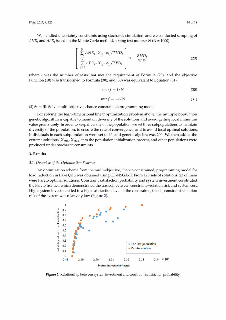
An optimization scheme from the multi-objective, chance-constrained, programming model forload reduction in Lake Qilu was obtained using CE-NSGA-II. From 120 sets of solutions, 23 of themwere Pareto optimal solutions. Constraint satisfaction probability and system investment constitutedthe Pareto frontier, which demonstrated the tradeoff between constraint-violation risk and system cost.High system investment led to a high satisfaction level of the constraints, that is, constraint-violationrisk of the system was relatively low (Figure 2).
Water 2017, 9, 322 10 of 17
3. Results
3.1. Overview of the Optimization Schemes
An optimization scheme from the multi-objective, chance-constrained, programming model for load reduction in Lake Qilu was obtained using CE-NSGA-II. From 120 sets of solutions, 23 of them were Pareto optimal solutions. Constraint satisfaction probability and system investment constituted the Pareto frontier, which demonstrated the tradeoff between constraint-violation risk and system cost. High system investment led to a high satisfaction level of the constraints, that is, constraint-violation risk of the system was relatively low (Figure 2).
Figure 2. Relationship between system investment and constraint satisfaction probability.
To represent and quantify the relationship between system investment and constraint satisfaction probability, the change rate index (CR) was introduced:
, 8 8
, ,
/10 ( ) /10m m n m n mv v v
m m n m m n m n mp p p
F F FCR
F F F
+ +
+ + +
Δ −= =Δ −
(32)
CR refers to the increment of system investment that corresponded to the constraint satisfaction probability from solution m to m + n, after sorting the system investment from small to large. The relationship between CR and FP indicated that there was a dramatic increment on system investment when constraint satisfaction probability was higher than 0.9 (Figure 3). Marginal effectiveness was obvious in schemes 3–7, in which a small investment reduced model risk significantly. Schemes 12–19 were ideal schemes, and decision-makers can consider flexible options regarding their preference for budget constraints or system stability.
Figure 3. Relationship between CR and constraint satisfaction probability for 19 Pareto solutions.
Figure 2. Relationship between system investment and constraint satisfaction probability.

Water 2017, 9, 322 11 of 18
To represent and quantify the relationship between system investment and constraint satisfactionprobability, the change rate index (CR) was introduced:
CRm,m+n =∆Fm,m+n
v /108
∆Fm,m+np
=(Fm+n
v − Fmv )/108
Fm+np − Fm
p(32)
CR refers to the increment of system investment that corresponded to the constraint satisfactionprobability from solution m to m + n, after sorting the system investment from small to large. Therelationship between CR and FP indicated that there was a dramatic increment on system investmentwhen constraint satisfaction probability was higher than 0.9 (Figure 3). Marginal effectiveness wasobvious in schemes 3–7, in which a small investment reduced model risk significantly. Schemes 12–19were ideal schemes, and decision-makers can consider flexible options regarding their preference forbudget constraints or system stability.
Water 2017, 9, 322 10 of 17
3. Results
3.1. Overview of the Optimization Schemes
An optimization scheme from the multi-objective, chance-constrained, programming model for load reduction in Lake Qilu was obtained using CE-NSGA-II. From 120 sets of solutions, 23 of them were Pareto optimal solutions. Constraint satisfaction probability and system investment constituted the Pareto frontier, which demonstrated the tradeoff between constraint-violation risk and system cost. High system investment led to a high satisfaction level of the constraints, that is, constraint-violation risk of the system was relatively low (Figure 2).
Figure 2. Relationship between system investment and constraint satisfaction probability.
To represent and quantify the relationship between system investment and constraint satisfaction probability, the change rate index (CR) was introduced:
, 8 8
, ,
/10 ( ) /10m m n m n mv v v
m m n m m n m n mp p p
F F FCR
F F F
+ +
+ + +
Δ −= =Δ −
(32)
CR refers to the increment of system investment that corresponded to the constraint satisfaction probability from solution m to m + n, after sorting the system investment from small to large. The relationship between CR and FP indicated that there was a dramatic increment on system investment when constraint satisfaction probability was higher than 0.9 (Figure 3). Marginal effectiveness was obvious in schemes 3–7, in which a small investment reduced model risk significantly. Schemes 12–19 were ideal schemes, and decision-makers can consider flexible options regarding their preference for budget constraints or system stability.
Figure 3. Relationship between CR and constraint satisfaction probability for 19 Pareto solutions. Figure 3. Relationship between CR and constraint satisfaction probability for 19 Pareto solutions.
3.2. Analysis on Optimal Solutions
Schemes 12–19 were optimal solutions for both system investment and constraint satisfaction(Figure 3). The solutions under six engineering measures are shown as Table 5, taking Hongqisub-watersheds, for example.
Table 5. Scale of measures for optimal schemes 12 to 19.
Watershed i Hongqi Sub-Watershed
Measure j SewageTreatment
DomesticRubbishDisposal
AgriculturalSewage Collection
and Treatment
Soil Testing andFormulatedFertilization
ConstructedWetlands
EcologicalRestoration
unit m3 t m3 hm2 hm2 hm2
12 4.1395 × 10⁹ 1.9095 × 10⁴ 4.5443 × 10⁸ 156.71 3.18 0.0513 4.1363 × 10⁹ 1.9095 × 10⁴ 4.6182 × 10⁸ 157.09 3.36 0.0514 4.1407 × 10⁹ 1.9095 × 10⁴ 4.6366 × 10⁸ 162.21 1.51 0.0715 4.1345 × 10⁹ 1.9095 × 10⁴ 4.7178 × 10⁸ 200.07 1.55 0.0816 4.1288 × 10⁹ 1.9095 × 10⁴ 4.7674 × 10⁸ 203.43 2.18 0.0817 4.1268 × 10⁹ 1.9095 × 10⁴ 5.1142 × 10⁸ 220.06 11.44 0.0618 4.0854 × 10⁹ 1.9095 × 10⁴ 5.0840 × 10⁸ 178.40 6.69 0.0819 4.1477 × 10⁹ 1.9095 × 10⁴ 5.7085 × 10⁸ 227.50 4.35 0.31
3.2.1. Sewage Treatment
Among the five sub-watersheds, only the Hongqi sub-watershed was suitable for establishing amunicipal sewage treatment plant, because the other four sub-watersheds were in rural regions, wheresewage disposal and constructed wetlands were used to treat sewage.

Water 2017, 9, 322 12 of 18
For the Hongqi sub-watershed (W1), there were no significant differences between the capacitiesof municipal wastewater treatment plants between schemes 12–17, although the project scale forsewage collection and disposal increased and constructed wetland areas decreased from schemes12–17. Schemes 18 and 19 exhibited differences from the others in size decline of sewage treatmentplants. In particular, the size of sewage treatment plants and sewage disposal projects in scheme 19were higher than for other schemes to ensure lower system risk (Figure 4).
Water 2017, 9, 322 11 of 17
3.2. Analysis on Optimal Solutions
Schemes 12–19 were optimal solutions for both system investment and constraint satisfaction (Figure 3). The solutions under six engineering measures are shown as Table 5, taking Hongqi sub-watersheds, for example.
Table 5. Scale of measures for optimal scheme 12 to 19.
Watershed i Hongqi Sub-Watershed
Measure j Sewage
Treatment
Domestic Rubbish Disposal
Agricultural Sewage Collection
and Treatment
Soil Testing and Formulated
Fertilization
Constructed Wetlands
Ecological Restoration
unit m3 t m3 hm2 hm2 hm2 12 4.1395 × 10⁹ 1.9095 × 10⁴ 4.5443 × 10⁸ 156.71 3.18 0.05 13 4.1363 × 10⁹ 1.9095 × 10⁴ 4.6182 × 10⁸ 157.09 3.36 0.05 14 4.1407 × 10⁹ 1.9095 × 10⁴ 4.6366 × 10⁸ 162.21 1.51 0.07 15 4.1345 × 10⁹ 1.9095 × 10⁴ 4.7178 × 10⁸ 200.07 1.55 0.08 16 4.1288 × 10⁹ 1.9095 × 10⁴ 4.7674 × 10⁸ 203.43 2.18 0.08 17 4.1268 × 10⁹ 1.9095 × 10⁴ 5.1142 × 10⁸ 220.06 11.44 0.06 18 4.0854 × 10⁹ 1.9095 × 10⁴ 5.0840 × 10⁸ 178.40 6.69 0.08 19 4.1477 × 10⁹ 1.9095 × 10⁴ 5.7085 × 10⁸ 227.50 4.35 0.31
3.2.1. Sewage Treatment
Among the five sub-watersheds, only the Hongqi sub-watershed was suitable for establishing a municipal sewage treatment plant, because the other four sub-watersheds were in rural regions, where sewage disposal and constructed wetlands were used to treat sewage.
For the Hongqi sub-watershed (W1), there were no significant differences between the capacities of municipal wastewater treatment plants between schemes 12–17, although the project scale for sewage collection and disposal increased and constructed wetland areas decreased from schemes 12–17. Schemes 18 and 19 exhibited differences from the others in size decline of sewage treatment plants. In particular, the size of sewage treatment plants and sewage disposal projects in scheme 19 were higher than for other schemes to ensure lower system risk (Figure 4).
Figure 4. Scale of sewage treatment measures in W1.
In W2 to W5 (Zhewan River sub-watershed, Zhong River sub-watershed, Daxin River sub-watershed, and Northest sub-watershed), the scale for sewage collection and disposal projects showed a small increase, and constructed wetlands increased significantly, because no municipal wastewater treatment plant has been built in these regions. The scale of constructed wetlands varied among different sub-watersheds, and decision-makers can choose alternatives by taking into account any practical issues they might encounter within a particular sub-watershed (sub-watershed 2, for example, shown in Figure 5).
Figure 4. Scale of sewage treatment measures in W1.
In W2 to W5 (Zhewan River sub-watershed, Zhong River sub-watershed, Daxin Riversub-watershed, and Northest sub-watershed), the scale for sewage collection and disposal projectsshowed a small increase, and constructed wetlands increased significantly, because no municipalwastewater treatment plant has been built in these regions. The scale of constructed wetlands variedamong different sub-watersheds, and decision-makers can choose alternatives by taking into accountany practical issues they might encounter within a particular sub-watershed (sub-watershed 2, forexample, shown in Figure 5).
Water 2017, 9, 322 12 of 17
Figure 5. Scale of sewage treatment measures in W2.
3.2.2. Load Reduction of TN and TP
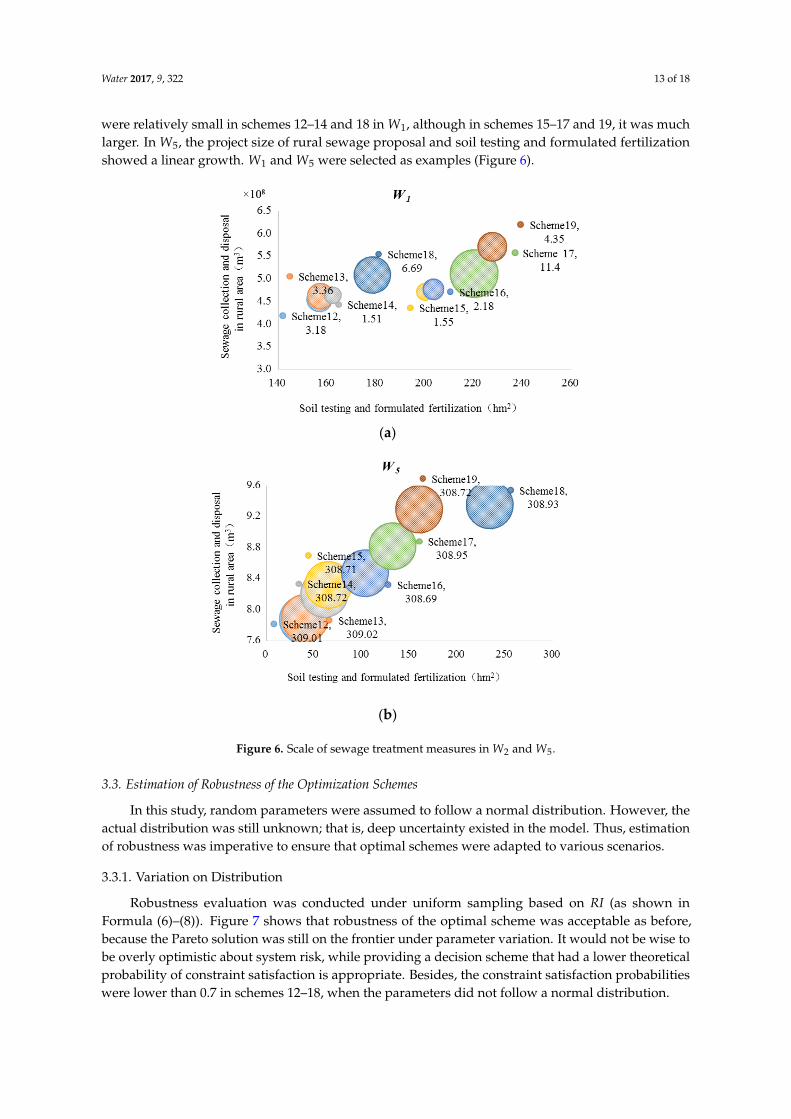
The scope of measures for TN and TP reduction was also provided in the optimal scheme. In W1, constructed wetlands were small-scale in each scheme, but the scale of sewage collection, soil testing, and formulated fertilization increased sharply. The scale of soil testing and formulated fertilization were relatively small in schemes 12–14 and 18 in W1, although in schemes 15–17 and 19, it was much larger. In W5, the project size of rural sewage proposal and soil testing and formulated fertilization showed a linear growth. W1 and W5 were selected as examples (Figure 6).
(a)
(b)
Figure 6. Scale of sewage treatment measures in W2 and W5.
Figure 5. Scale of sewage treatment measures in W2.
3.2.2. Load Reduction of TN and TP
The scope of measures for TN and TP reduction was also provided in the optimal scheme. In W1,constructed wetlands were small-scale in each scheme, but the scale of sewage collection, soil testing,and formulated fertilization increased sharply. The scale of soil testing and formulated fertilization
Water 2017, 9, 322 13 of 18
were relatively small in schemes 12–14 and 18 in W1, although in schemes 15–17 and 19, it was muchlarger. In W5, the project size of rural sewage proposal and soil testing and formulated fertilizationshowed a linear growth. W1 and W5 were selected as examples (Figure 6).
Water 2017, 9, 322 12 of 17
Figure 5. Scale of sewage treatment measures in W2.
3.2.2. Load Reduction of TN and TP
The scope of measures for TN and TP reduction was also provided in the optimal scheme. In W1, constructed wetlands were small-scale in each scheme, but the scale of sewage collection, soil testing, and formulated fertilization increased sharply. The scale of soil testing and formulated fertilization were relatively small in schemes 12–14 and 18 in W1, although in schemes 15–17 and 19, it was much larger. In W5, the project size of rural sewage proposal and soil testing and formulated fertilization showed a linear growth. W1 and W5 were selected as examples (Figure 6).
(a)
(b)
Figure 6. Scale of sewage treatment measures in W2 and W5. Figure 6. Scale of sewage treatment measures in W2 and W5.
3.3. Estimation of Robustness of the Optimization Schemes
In this study, random parameters were assumed to follow a normal distribution. However, theactual distribution was still unknown; that is, deep uncertainty existed in the model. Thus, estimationof robustness was imperative to ensure that optimal schemes were adapted to various scenarios.
3.3.1. Variation on Distribution
Robustness evaluation was conducted under uniform sampling based on RI (as shown inFormula (6)–(8)). Figure 7 shows that robustness of the optimal scheme was acceptable as before,because the Pareto solution was still on the frontier under parameter variation. It would not be wise tobe overly optimistic about system risk, while providing a decision scheme that had a lower theoreticalprobability of constraint satisfaction is appropriate. Besides, the constraint satisfaction probabilitieswere lower than 0.7 in schemes 12–18, when the parameters did not follow a normal distribution.

Water 2017, 9, 322 14 of 18
Water 2017, 9, 322 13 of 17
3.3. Estimation of Robustness of the Optimization Schemes
In this study, random parameters were assumed to follow a normal distribution. However, the actual distribution was still unknown; that is, deep uncertainty existed in the model. Thus, estimation of robustness was imperative to ensure that optimal schemes were adapted to various scenarios.
3.3.1. Variation on Distribution
Robustness evaluation was conducted under uniform sampling based on RI (as shown in Formula (6)–(8)). Figure 7 shows that robustness of the optimal scheme was acceptable as before, because the Pareto solution was still on the frontier under parameter variation. It would not be wise to be overly optimistic about system risk, while providing a decision scheme that had a lower theoretical probability of constraint satisfaction is appropriate. Besides, the constraint satisfaction probabilities were lower than 0.7 in schemes 12–18, when the parameters did not follow a normal distribution.
Figure 7. Relationship between system investment and constraint satisfaction probability when stochastic parameters obey uniform distribution.
3.3.2. Variation in Mean Values of the Parameters
Mean values of parameters were obtained from actual measurements or estimations, which also brought uncertainties. Therefore, robustness evaluations on the optimal schemes based on different mean values evaluation was carried out. New mean values of ANRj and APRj, which decreased by 10%, are shown in Formula (33) and (34):
(1 10%)j jANR ANRμ μ∗ = × − (33)
(1 10%)j jAPR APRμ μ∗ = × − (34)
According to the new mean values, the relationship between system investment and constraint satisfaction probability under the new distribution was obtained (Figure 8). The result indicated that robustness of the optimal scheme was very good. Not only were the solutions still on the Pareto frontier, but also the marginal effect of system investment on the constraint satisfaction probability increased rapidly.
New mean values of ANRj and APRj that increased by 10% are shown in Formula (35) and (36):
(1 10%)j jANR ANRμ μ∗ = × + (35)
Figure 7. Relationship between system investment and constraint satisfaction probability whenstochastic parameters obey uniform distribution.
3.3.2. Variation in Mean Values of the Parameters
Mean values of parameters were obtained from actual measurements or estimations, which alsobrought uncertainties. Therefore, robustness evaluations on the optimal schemes based on differentmean values evaluation was carried out. New mean values of ANRj and APRj, which decreased by10%, are shown in Formula (33) and (34):
µ∗ANRj= µANRj × (1− 10%) (33)
µ∗APRj= µAPRj × (1− 10%) (34)
According to the new mean values, the relationship between system investment and constraintsatisfaction probability under the new distribution was obtained (Figure 8). The result indicated thatrobustness of the optimal scheme was very good. Not only were the solutions still on the Paretofrontier, but also the marginal effect of system investment on the constraint satisfaction probabilityincreased rapidly.
Water 2017, 9, 322 14 of 17
(1 10%)j jAPR APRμ μ∗ = × + (36)
Figure 8. Relationship between system investment and constraint satisfaction probability when the mean values of stochastic parameters decrease by 10%.
The new relationship between system investment and constraint satisfaction probability under the new distribution is shown in Figure 9, and the result shows that solutions were still on the Pareto frontier, that is, the scheme was robust. However, it is inappropriate to be overly optimistic about a constraint satisfaction probability that was obtained in the optimal scheme.
Figure 9. Relationship between system investment and constraint satisfaction probability when the mean values of stochastic parameters increase by 10%.
4. Discussion
The multi-objective chance-constrained programming approach integrated with GA and robustness estimation has been provided and applied to a nutrient load reduction problem within the watershed of Plateau Lake. The methodology proposed in this article can present and deal with multi-objective and random information of the system (expressed in minimize system cost and maximize water qualification rate), evaluate robustness of the optimal solutions obtained by GA, and shows the following advantages for making decisions about optimal nutrient load reduction:
(a) Multi-objective, chance-constrained, programming has the ability to trade off various optimal objectives in real cases, such as the minimal system cost and maximization of constraint
Figure 8. Relationship between system investment and constraint satisfaction probability when themean values of stochastic parameters decrease by 10%.
Water 2017, 9, 322 15 of 18
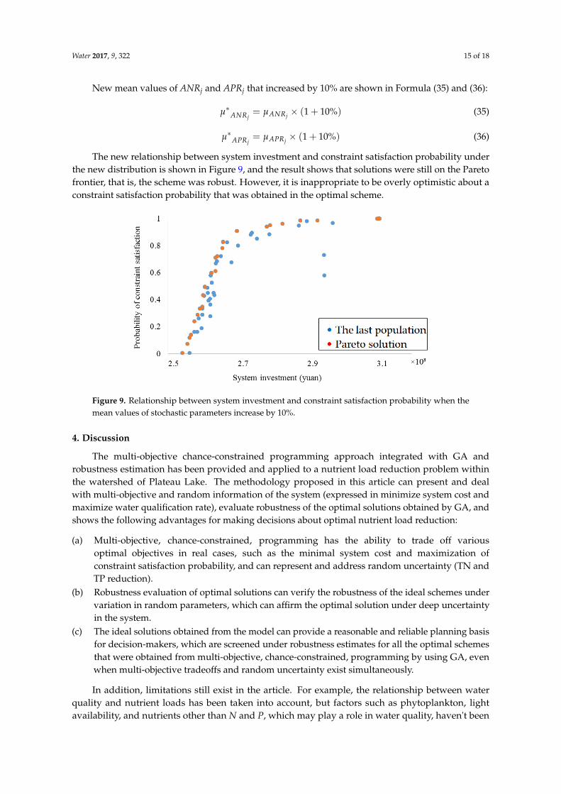
New mean values of ANRj and APRj that increased by 10% are shown in Formula (35) and (36):
µ∗ANRj= µANRj × (1 + 10%) (35)
µ∗APRj= µAPRj × (1 + 10%) (36)
The new relationship between system investment and constraint satisfaction probability underthe new distribution is shown in Figure 9, and the result shows that solutions were still on the Paretofrontier, that is, the scheme was robust. However, it is inappropriate to be overly optimistic about aconstraint satisfaction probability that was obtained in the optimal scheme.
Water 2017, 9, 322 14 of 17
(1 10%)j jAPR APRμ μ∗ = × + (36)
Figure 8. Relationship between system investment and constraint satisfaction probability when the mean values of stochastic parameters decrease by 10%.
The new relationship between system investment and constraint satisfaction probability under the new distribution is shown in Figure 9, and the result shows that solutions were still on the Pareto frontier, that is, the scheme was robust. However, it is inappropriate to be overly optimistic about a constraint satisfaction probability that was obtained in the optimal scheme.
Figure 9. Relationship between system investment and constraint satisfaction probability when the mean values of stochastic parameters increase by 10%.
4. Discussion
The multi-objective chance-constrained programming approach integrated with GA and robustness estimation has been provided and applied to a nutrient load reduction problem within the watershed of Plateau Lake. The methodology proposed in this article can present and deal with multi-objective and random information of the system (expressed in minimize system cost and maximize water qualification rate), evaluate robustness of the optimal solutions obtained by GA, and shows the following advantages for making decisions about optimal nutrient load reduction:
(a) Multi-objective, chance-constrained, programming has the ability to trade off various optimal objectives in real cases, such as the minimal system cost and maximization of constraint
Figure 9. Relationship between system investment and constraint satisfaction probability when themean values of stochastic parameters increase by 10%.
4. Discussion
The multi-objective chance-constrained programming approach integrated with GA androbustness estimation has been provided and applied to a nutrient load reduction problem withinthe watershed of Plateau Lake. The methodology proposed in this article can present and dealwith multi-objective and random information of the system (expressed in minimize system cost andmaximize water qualification rate), evaluate robustness of the optimal solutions obtained by GA, andshows the following advantages for making decisions about optimal nutrient load reduction:
(a) Multi-objective, chance-constrained, programming has the ability to trade off variousoptimal objectives in real cases, such as the minimal system cost and maximization ofconstraint satisfaction probability, and can represent and address random uncertainty (TN andTP reduction).
(b) Robustness evaluation of optimal solutions can verify the robustness of the ideal schemes undervariation in random parameters, which can affirm the optimal solution under deep uncertaintyin the system.
(c) The ideal solutions obtained from the model can provide a reasonable and reliable planning basisfor decision-makers, which are screened under robustness estimates for all the optimal schemesthat were obtained from multi-objective, chance-constrained, programming by using GA, evenwhen multi-objective tradeoffs and random uncertainty exist simultaneously.
In addition, limitations still exist in the article. For example, the relationship between waterquality and nutrient loads has been taken into account, but factors such as phytoplankton, lightavailability, and nutrients other than N and P, which may play a role in water quality, haven't been

Water 2017, 9, 322 16 of 18
considered. In future research, influences from the factors above should be further considered andadded into the model, so that the robustness of the methodology can be enhanced.
5. Conclusions
A multi-objective, chance-constrained, programming approach has been proposed by integratingMOP and CCP with GA and robustness estimation, which can balance the conflict between multipleoptimal objectives and deal with random uncertainty within the system simultaneously. GA androbustness estimation were combined in multi-objective, chance-constrained, programming to acquireoptimization schemes and to provide robust, optimal decisions. The model was applied to the optimalnutrient load reduction in the Lake Qilu watershed, which performed satisfactorily in balancingminimal system cost with maximization of constraint satisfaction probability, and in handling randomuncertainty at the same time.
Ideal schemes obtained from this optimization model reflected the relationship between systeminvestment and risk, and indicated that high system investment led to high satisfaction level with theconstraints. Under the ideal schemes, detailed analysis was conducted in five sub-watersheds undersix engineering measures on sewage treatment and reduction of TN and TP. Further, an evaluation ofthe robustness of the scheme was implemented, and the results demonstrated that the ideal schemeshave superior robustness under uncertainty. This study is the first attempt to optimize reduction ofwatershed nutrient loads by using multi-objective, chance-constrained, programming, and it can alsobe applicable to other areas to manage the reduction of nutrient loads.
Acknowledgments: This paper was supported by the National Basic Research Program of China (2015CB458900)and the China National Water Pollution Control Program (2013ZX07102-006). We appreciate Thomas A. Gavin atCornell University for help with editing the English in this paper.
Author Contributions: Yao Ji and Xujun Liu designed framework of the article; Mengjiao Zhang, Han Su, FeifeiDong and Yong Liu analyzed the data; Xujun Liu and Yao Ji wrote the paper.
Conflicts of Interest: The authors declare no conflict of interest.
References
1. Liu, Y.; Guo, H.C.; Zhou, F.; Wang, L.J.; Zhang, X.M.; He, B. Watershed approach as a framework forlake-watershed pollution control. Acta Sci. Circumst. 2006, 26, 337–344.
2. Yan, H.Y.; Huang, Y.; Wang, G.Y. Water eutrophication evaluation based on rough set and petri nets: A casestudy in Xiangxi-River, Three Gorges Reservoir. Ecol. Indic. 2016, 69, 463–472. [CrossRef]
3. Dai, C.; Tan, Q.; Lu, W.T.; Liu, Y.; Guo, H.C. Identification of optimal water transfer schemes for restorationof a eutrophic lake: An integrated simulation-optimization method. Ecol. Eng. 2016, 95, 409–421. [CrossRef]
4. Conley, D.J.; Paerl, H.W.; Howarth, R.W.; Boesch, D.F.; Seitzinger, S.P.; Havens, K.E.; Lancelot, C.; Likens, G.E.Controlling eutrophication: Nitrogen and phosphorus. Science 2009, 323, 1014–1015. [CrossRef] [PubMed]
5. Li, Y.P.; Tang, C.Y.; Yu, Z.B.; Acharya, K. Correlations between algae and water quality: Factors drivingeutrophication in Lake Taihu, China. Int. J. Environ. Sci. Technol. 2014, 11, 169–182. [CrossRef]
6. Ahlvik, L.; Ekholm, P.; Hyytiäinen, K.; Pitkänen, H. An economic-ecological model to evaluate impacts ofnutrient abatement in the Baltic Sea. Environ. Model. Softw. 2014, 55, 164–175. [CrossRef]
7. Wang, Z.; Zou, R.; Zhu, X.; Yuan, G.; Zhao, L.; Liu, Y. Predicting lake water quality responses to loadreduction: A three-dimensional modeling approach for total maximum daily load. Int. J. Environ. Sci. Technol.2011, 11, 423–436. [CrossRef]
8. Liu, Y.; Zou, R.; Guo, H.C. Intelligent Watershed Management; Science Press: Beijing, China, 2012.9. Liu, Y.; Zou, R.; Riverson, J.; Yang, P.J.; Guo, H.C. Guided adaptive optimal decision making approach for
uncertainty based watershed scale load reduction. Water Res. 2014, 45, 4885–4895. [CrossRef] [PubMed]10. Dong, F.F.; Liu, Y.; Qian, L.; Sheng, H.; Yang, Y.H.; Guo, H.C.; Zhao, L. Interactive decision procedure for
watershed nutrient load reduction: An integrated chance-constrained programming model with risk-costtradeoff. Environ. Model. Softw. 2014, 61, 166–173. [CrossRef]
11. Tang, C.Y.; Li, Y.P.; Acharya, K. Modeling the effects of external nutrient reductions on algal blooms inhyper-eutrophic Lake Taihu, China. Ecol. Eng. 2016, 94, 164–173. [CrossRef]
Water 2017, 9, 322 17 of 18
12. Fonseca, A.; Botelho, C.; Boaventura, R.A.R.; Vilar, V.J.P. Integrated hydrological and water quality modelfor river management: A case study on Lena River. Sci. Total Environ. 2014, 485–486, 474–489. [CrossRef][PubMed]
13. Mittelstet, A.R.; Storm, D.E.; White, M.J. Using SWAT to enhance watershed-based plans to meet numericwater quality standards. Sustain. Water Qual. Ecol. 2016, 7, 5–21. [CrossRef]
14. Yang, G.X.; Best, E.P.H. Spatial optimization of watershed management practices for nitrogen load reductionusing a modeling-optimization framework. J. Environ. Manag. 2015, 161, 252–260. [CrossRef] [PubMed]
15. Chen, J.D.; Dahlgren, R.A.; Shen, Y.N.; Lu, J. A Bayesian approach for calculating variable total maximumdaily loads and uncertainty assessment. Sci. Total Environ. 2012, 430, 59–67. [CrossRef] [PubMed]
16. Wu, S.M.; Huang, G.H.; Guo, H.C. An interactive inexact-fuzzy approach for multi-objective planning ofwater environmental systems. Water Sci. Technol. 1997, 36, 235–242. [CrossRef]
17. Kumar, R.S.; Kondapaneni, K.; Dixit, V.; Goswami, A.; Thakur, L.S.; Tiwari, M.K. Multi-objective modeling ofproduction and pollution routing problem with time window: A self-learning particle swarm optimizationapproach. Comput. Ind. Eng. 2016, 99, 29–40. [CrossRef]
18. Bostian, M.; Whittaker, G.; Barnhart, B.; Färe, R.; Grosskopf, S. Valuing water quality tradeoffs at differentspatial scales: An integrated approach using bilevel optimization. Water Resour. Econ. 2015, 11, 1–12.[CrossRef]
19. Guariso, G.; Pirovano, G.; Volta, M. Multi-objective analysis of ground-level ozone concentration control.J. Environ. Manag. 2004, 71, 25–33. [CrossRef] [PubMed]
20. Li, P.; Arellano-Garcia, H.; Wozny, G. Chance constrained programming approach to process optimizationunder uncertainty. Comput. Chem. Eng. 2008, 32, 25–45. [CrossRef]
21. Ji, Y.; Huang, G.H.; Sun, W. Inexact left-hand-side chance-constrained programming for nonpoint-sourcewater quality management. Water Air Soil Pollut. 2014, 225, 1895–1908. [CrossRef]
22. Ji, Y.; Huang, G.H.; Sun, W. Nonpoint-Source Water Quality Management under Uncertainty through anInexact Double-Sided Chance-Constrained Model. Water Resour. Manag. 2015, 29, 3079–3094. [CrossRef]
23. “The Twelfth Five Year Plan” for Water Pollution Control in Qilu Lake Watershed. [EB/OL].Available online: http://xxgk.yn.gov.cn/Z_M_013/Info_Detail.aspx?DocumentKeyID=5CCDC5632E7847E8B38C6DB39EA575DA (accessed on 16 March 2011).
24. Charnes, A.; Cooper, W.W. Chance-constrained programming. Manag. Sci. 1959, 6, 73–79. [CrossRef]25. Bes, C.; Sethi, S. Solution of a class of stochastic linear-convex control problems using deterministic
equivalents. J. Optimiz. Theor. Appl. 1989, 62, 17–27. [CrossRef]26. Liu, B.; Iwamura, K. Chance constrained programming with fuzzy parameters. Fuzzy Sets Syst. 1998, 94,
227–237. [CrossRef]27. Qin, X.; Huang, G.; Liu, L. A genetic-algorithm-aided stochastic optimization model for regional air quality
management under uncertainty. J. Air Waste Manag. Assoc. 2010, 60, 63–71. [CrossRef] [PubMed]28. Biswal, M.P.; Li, D. Probabilistic linear programming problems with exponential random variables:
A technical note. Eur. J. Oper. Res. 1998, 111, 589–597. [CrossRef]29. Goicoechea, A.; Duckstein, L. Nonnormal deterministic equivalents and a transformation in stochastic
mathematical programming. Appl. Math. Comput. 1987, 21, 51–72. [CrossRef]30. Lux, I.; Koblinger, L. Monte Carlo particle transport methods: Neutron and photon calculations.
Appl. Math. Comput. 1987, 26, 369–395.31. Marler, R.T.; Arora, J.S. Survey of multi-objective optimization methods for engineering.
Struct. Multidiscip. Optim. 2004, 21, 51–72. [CrossRef]32. Coello, C. A comprehensive survey of evolutionary-based multiobjective optimization techniques. Knowl.
Inf. Syst. 1999, 1, 269–308. [CrossRef]33. Liu, G.H.; Bao, H.; Li, W.C. A Genetic Algorithm in MATLAB. Appl. Res. Comput. 2001, 18, 80–82.34. Deb, K.; Agrawal, S.; Pratap, A.; Meyarivan, T. A fast elitist non-dominated sorting genetic algorithm for
multi-objective optimization: NSGA-II. Lect. Notes Comput. Sci. 2000, 1917, 849–858.35. Maity, S.; Roy, A.; Maiti, M. An imprecise Multi-Objective Genetic Algorithm for uncertain Constrained
Multi-Objective Solid Travelling Salesman Problem. Exp. Syst. Appl. 2015, 46, 196–223. [CrossRef]36. Shi, R.F. Studies on Multi-Objective Evoluationary Algorithms with Applications to Production Scheduling; Baihang
University: Beijing, China, 2006.

Water 2017, 9, 322 18 of 18
37. Abul’Wafa, A.R. Optimization of economic/emission load dispatch for hybrid generating systems usingcontrolled Elitist NSGA-II. Electr. Power Syst. Res. 2013, 105, 142–151. [CrossRef]
38. Hashimoto, T.; Stedinger, J.R.; Loucks, D.P. Reliability, resiliency, and vulnerability criteria for water resourcesystem performance evaluation. Water Resour. Res. 1982, 18, 14–20. [CrossRef]
39. Bankes, S.C. Tools and techniques for developing policies for complex and uncertain systems. Proc. Natl.Acad. Sci. USA 2002, 99, 7263–7266. [CrossRef] [PubMed]
40. Walker, W.E.; Lempert, R.J.; Kwakkel, J.H. Deep Uncertainty. Encycl. Oper. Res. Manag. Sci. 2016, 395–402.[CrossRef]
41. Watkins, D.W.; McKinney, D.C. Finding robust solutions to water resources problems. J. Water Resour.Plan. Manag. 1997, 123, 49–58. [CrossRef]
42. Shi, W.Q. Modeling about Hydrochemical Variation of Tangpu Reservoir Watershed and Total Pollution AmountControl; Zhejiang University: Hangzhou, China, 2014.
43. Fu, B.; Liu, H.B.; Lu, Y.; Zhai, L.M.; Jin, G.M.; Li, W.C.; Duan, Z.Y.; Hu, W.L.; Lei, Q.L. Study on characteristicsof nitrogen and phosphorus emission in typical small watershed of plateau lakes: A case study of the FengyuRiver Watershed. Acta Sci. Circum. 2015, 9, 2892–2899. (In Chinese)
© 2017 by the authors. Licensee MDPI, Basel, Switzerland. This article is an open accessarticle distributed under the terms and conditions of the Creative Commons Attribution(CC BY) license (http://creativecommons.org/licenses/by/4.0/).