a multi-phase, flexible, and accurate lattice for pricing complex derivatives with multiple market...
TRANSCRIPT
A Multi-Phase, Flexible, and Accurate Lattice for Pricing
Complex Derivatives with Multiple Market Variables
BTT(Bino-trinomial Tree)
• A method can reduce nonlinearity error.• The nonlinearity occurs at certain critical
locations such as a certain point, a price level, or a time point.
• Pricing results converge smoothly and quickly.• A BTT is combined a more bBTT(basic BTT)

bBTT(Basic Bino-trinomial Tree)
• The bBTT is essentially a binomial tree except for a trinomial structure at the first time step.
• There is a truncated CRR tree at the second time step to maturity.
• Which provides the needed flexibility to deal with critical locations.

Basic Terms
• The stock price follow a lognormal diffusion process:
=> • The mean and variance of the lognormal
return of :
• The CRR(Cox, Ross, & Rubinstein) lattice adopts: ,
,
t t
r t r t
u d
u e d e
e d u eP P
u d u d
( )S t
( )S t

Log-distance
• Define the log-distance between stock price and as .• The log-distance between any two adjacent
stock price at any time step in the CRR lattice is .
1S 2S 1 2| ln ln |S S
2 t
ln ln ln ln
ln ln
( )
2
t t
Su Sd u d
e e
t t
t

CRR tree

bBTT

bBTT
• Coincide the lattices and the barriers.• Let • Adjust s.t to be an integer.• The first time interval
2
h l
t
t
' 1 ( ' > )T
t T t t tt
ln( ) ln( ) s s
H Lh and l
S S

The probability of the latticesat first step time
The probability of the latticesat first step time
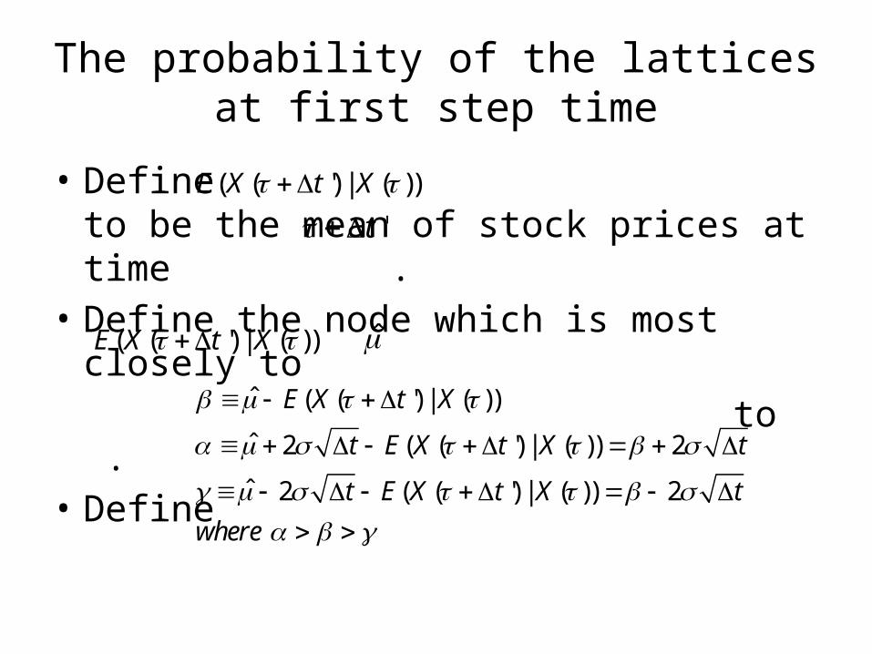
• Define to be the mean of stock prices at time .
• Define the node which is most closely to to .• Define
( ( ') | ( ))E X t X
't
( ( ') | ( ))E X t X ̂
ˆ ( ( ') | ( ))
ˆ 2 ( ( ') | ( )) 2
ˆ 2 ( ( ') | ( )) 2
E X t X
t E X t X t
t E X t X t
where

The probability of the latticesat first step time
• The branching probabilities of node A can be derived by solving the equalities:
( . ., , , )u m di e P P P

The probability of the latticesat first step time
• By Cramer’s rule, we solve it as
Transform correlated processes to uncorrelated
• Use the orthogonalization to transform a set of correlated process to uncorrelated.
• Construct a lattice for the first uncorrelated process which match the first coordinate.
• Then construct the second uncorrelated process on the first lattice to form a bivariate lattice which match the second coordinate.
• For general, the i-th uncorrelated process on top of the (i-1)-variate lattice constructed an i-variate lattice. The i-th lattice match the i-th coordinate.

Transform correlated processes to uncorrelated
• Demonstrate for 2 correlated processes.• Let and follow:
• can be decomposed into a linear combination of and another independent Brownian motion :
1S 2S
2dz
1dz
dz

Transform correlated processes to uncorrelated
• The matrix form:
• Define =>
1
22 2
0
1A
11
2 21 2
1 0
1
1 1
A

Transform correlated processes to uncorrelated
• Transform and into two uncorrelated processes and .
• The matrix form:1X 2X
1S 2S
1
11 11
1 22 22 2
1 2
1
1 1
1 2
2 21 2
1 1
1 0
0 1
1 1
dS
dX dSA
dS dSdX dS
dzdt
dz
Transform correlated processes to uncorrelated
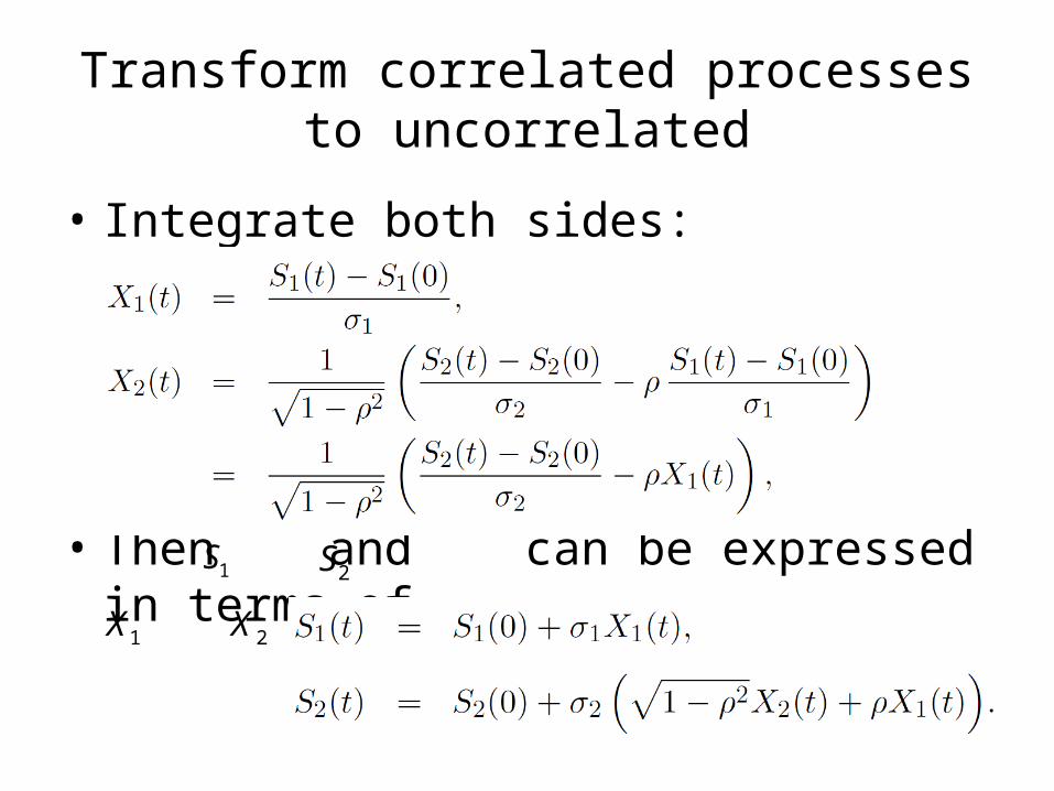
• Integrate both sides:
• Then and can be expressed in terms of and :
1S 2S
1X 2X

Multi-phase branch construction

A bivariate lattice: two correlated market variables
• Define is the stock price, is the firm’s asset value.
• The bivariate lattice is built to price vulnerable barrier options with the strike price and the barrier .
• The default boundary for the firm's asset value where
( )S t ( )V t
K( )( ) T tB t Be
* ( )( ( ), ) ( ( ), )r T tD S t t De c S t t

A bivariate lattice: two correlated market variables
• Assume and follow the processes:
• By Ito’s lemma:
( )S t ( )V t

A bivariate lattice: two correlated market variables
• Use the orthogonalization:
=>
ln
ln
ln ln
2 2ln ln
1 0
0 1
1 1
S
S S
S V
S V
dzdXdt
dY dz

Transform to( )B t ( )XB t
1 11
1
( ) (0)( )
ln ( ) ln (0)( ) ( )X
S
S t SX t
B t SB t

Transform to*( )D t * ( )YD t
2 22 12
2
**
2
( ) (0)1( ) ( )
1
1 ln ( ) ln (0)( ) ( )
1Y
V
S t SX t X t
D t VD t X t

The branches

An example lattice
• Assumption:
0
0
30
3
40
20%
100
20%
S
V
K
T
S
V
0
5%
75%
35
0.01
90
r
B
D

An example lattice
• Set the option for 2 periods ( ).• Compute the lattices in X coordinate first.• For example, • • • The log-distance between 2 vertically
adjacent nodes is•
1.5t
( )ln ( ) ln (0)( ) , ( ) sX t
s
S t SX t S t e
0.2 ( 0.743)(1.5) 34.479S e
2 2.45t
1.5t
21 0.2(1.5) 0.05 1.5 0.225
0.2 2
(1.5)
X
XXB

An example lattice
• • Similar,• • •
(1.5) 1.707, (1.5) 3.192, (1.5) 56.275, (1.5) 21.125u d u dX X S S 0.01 (3 3)ln(35 ) ln(40)
(3) 0.6680.2X
eB
(3) (1.5) (1.5) 1.707 0.225 1.932X u XX
(3) 0.668 2.45 1.782, (3) 1.782 2.45 4.231m uX X
(3) 93.237, (3) 57.125, (3) 35u m dS S S

An example lattice
• Then compute the lattices in Y coordinate.• For example,• •
0.05(1.5)1 2( (1.5),1.5) (1.5) ( ) 30 ( ) 28.019u uc S S N d e N d
* 0.05 1.5(1.5) 90 28.019 111.516D e
* 1 ln(111.516) ln(100)(1.5) 0 1.707 0.545
0.21 0YD

An example lattice
• Similar, • • • • •
0.05(3-3)1 2( (3),3) (3) ( ) 30 ( ) 63.237u uc S S N d e N d
* 0.05 (3-3)(3) 90 63.237 153.237uD e
0.05(3-3)1 2( (3),3) (3) ( ) 30 ( ) 27.125m mc S S N d e N d
* 0.05 (3-3)(3) 90 27.125 117.125mD e
* 1 ln(153.237) ln(100)(3) 0 4.231 2.134
0.21 0uYD
* 1 ln(117.125) ln(100)(3) 0 1.782 0.790
0.21 0dYD

An example lattice

An example lattice
• Plot the 3D coordinate by X, Y, and t.• Find , , and for the same method, which
• Compute the option value at each node.• Find the initial option value by backward
induction.
iY iV iQ
, , or i u m d

An example lattice
• For node C,
• For node D,• Then the call value at node B:
• By backward induction, the initial value=7.34
1
2
3
( (3) ) 63.237
0.75 ( (3) ) 47.43
93.890.75 ( (3) ) 29.06
153.237
u
u
u
c S K
c S K
c S K
1 2 327.13, 27.13, 20.34d d d
-

An example lattice

The Hull-While interest rate model
• The short rate at time t, r(t) follows
• is a function of time that make the model fit the real-world interest rate market.
• denotes the mean reversion rate for the short rate to revert to .
• denotes the instantaneous volatility of the short rate.
• is the standard Brownian motion.
( ) ( ( ) ( )) r rdr t t ar t dt dz
( )t
a( )r t ( )t
a
r
rdz
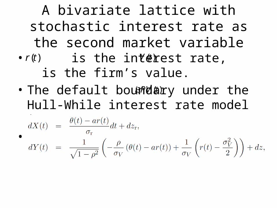
A bivariate lattice with stochastic interest rate as the second market variable
• is the interest rate, is the firm’s value.• The default boundary under the Hull-While
interest rate model is ,• The stochastic process:
( )r t ( )V t
( )PV t