a multicore neuromorphic chip design using multilevel
TRANSCRIPT
A Multicore Neuromorphic Chip Design Using Multilevel
Synapses in 65nm Standard CMOS Technology
A THESIS
SUBMITTED TO THE FACULTY OF THE GRADUATE SCHOOL
OF THE UNIVERSITY OF MINNESOTA
BY
Deepak Kumar Shivsharnappa Tagare
IN PARTIAL FULFILLMENT OF THE REQUIREMENTS
FOR THE DEGREE OF
MASTER OF SCIENCE IN ELECTRICAL ENGINEERING
Prof. Chris H. Kim
June 2015

© Deepak Kumar Shivsharnappa Tagare 2015

i
Acknowledgements
I would like to express my sincere gratitude to my advisor, Prof. Chris H. Kim for
giving me an opportunity to work with him. His unmatched teaching has always been a
source of inspiration and a reason to develop my interest towards the subject. His teaching
helped to get best out of me. I am thankful to him for his valuable time spent in guiding
and helping me to improve.
I am privileged being part of VLSI research lab at U of M. Having most dedicated
and humble colleagues around, I could learn a lot from them. My Sincere thanks to
Jongyeon Kim, this work wouldn’t have been possible without his support. He has been
like an elder brother to me. I am also thankful to Weichao Xu for helping me during initial
phase of this project.
I am grateful to all my friends and colleagues whom I met at my work places: Wipro
Technologies, Qualcomm and Intel Corporation. Their actions and decisions have
constantly helped me to improve myself and dream big. I would also want to thank all my
seniors and friends at U of M. Their encouragement has always helped me to take strong
decisions. Their presence made this place lively.
Most importantly, I would like to thank my parents and my brothers for their love,
support, guidance and sacrifices. I wouldn’t have realized my dream without their support.
My sincere gratitude to my uncle Dr. Suryakanth Gangshetty for his encouragement.

ii
This thesis is dedicated to my parents,
iii
Abstract
Neuromorphic research community is focused on designing a hardware which is as
efficient as biological brain in terms of performance, power and area. It opens up
opportunities to optimize these designs at all levels from architecture to devices. We
propose a novel architecture to have tight integration between neurons and synapses. Our
32K bit neuromorphic chip with 256 axons and 256 neurons demonstrates 4 neuromorphic
cores operating in a completely parallel fashion. Eflash memory core representing synapses
saves power and area. The Non-volatility of eflash consumes zero static power. The ability
to store multi-levels of weights in a single cell makes the array denser. Unlike flash
technology, eflash doesn’t require specialized fabrication process, hence the neuromorphic
chip is implemented in 65nm standard CMOS technology. The current sensing neurons
with parallel reading scheme makes the neuronal operation several orders of magnitude
faster than state-of-the-art neuromorphic designs. A generic design style of the
neuromorphic chip can demonstrate various neural network algorithms. As a proof-of-
concept, we implemented Restricted Boltzmann Machine (RBM) algorithm in our chip to
demonstrate handwritten digit recognition application.

iv
Table of Contents
List of figures ..................................................................................................................... v
Chapter 1 Introduction..................................................................................................... 1
Chapter 2 Application ...................................................................................................... 4
2.1 Restricted Boltzmann Machine (RBM) based learning ......................................................... 5
2.2 Spike generation using neuromorphic core ............................................................................ 6
2.3 Digit recognition using a classifier ........................................................................................ 6
Chapter 3 Algorithm and training .................................................................................. 9
Chapter 4 Architecture and design ............................................................................... 15
4.1 Neuronal dynamics .............................................................................................................. 15
4.2 Multicore design .................................................................................................................. 17
4.3 Current based reading scheme ............................................................................................. 19
4.4 Design floorplan................................................................................................................... 21
Chapter 5 Simulation results ......................................................................................... 23
5.1 Accuracy trend with varying number of neurons ................................................................. 23
5.2 Accuracy as a function of image size................................................................................... 24
5.3 Impact of weight levels on accuracy .................................................................................... 26
5.4 Grayscale vs binary pixel images ........................................................................................ 29
5.5 Accuracy trend with different number of cores ................................................................... 30
5.6 Error tolerant design ............................................................................................................ 31
5.7 HSPICE simulation results .................................................................................................. 33
Chapter 6 Conclusion ..................................................................................................... 36
Bibliography .................................................................................................................... 37

v
List of figures
Figure 2.1 Flow diagram of image recognition algorithm .................................................. 5
Figure 2.2 16x16 pixel image with grayscale and binary values ........................................ 7
Figure 2.3 Distribution of pixel values for grayscale and binary images ........................... 7
Figure 2.4 Digit recognition using classifier....................................................................... 8
Figure 3.1 RBM network .................................................................................................. 10
Figure 3.2 Learning using contrastive divergence ............................................................ 11
Figure 3.3 Distribution of real number weight matrix ...................................................... 13
Figure 3.4 Distribution of integer weight matrix .............................................................. 14
Figure 4.1 Architecture of neuromorphic core ................................................................. 16
Figure 4.2 Multicore design .............................................................................................. 18
Figure 4.3 Current based reading scheme ......................................................................... 20
Figure 4.4 Chip floorplan .................................................................................................. 22
Figure 5.1 Digit recognition accuracy vs number of neurons ........................................... 24
Figure 5.2 Digits of different pixel sizes .......................................................................... 25
Figure 5.3 Digit recognition accuracy vs number of pixels .............................................. 26
Figure 5.4 Comparison of accuracies for different weight levels ..................................... 27
Figure 5.5 Digit recognition accuracy vs weight levels .................................................... 28
Figure 5.6 Digit recognition accuracy with grayscale and binary images ........................ 29
Figure 5.7 Digit recognition accuracy vs number of cores ............................................... 30
Figure 5.8 Digit recognition accuracy vs spike errors ...................................................... 32
Figure 5.9 Internal current verification ............................................................................. 33

vi
Figure 5.10 Neuron operation ........................................................................................... 34
Figure 5.11 Gaussian distribution of offset current .......................................................... 35

1
Chapter 1 Introduction
The mysterious engineering behind a mammalian brain has been an inspiration for
cognitive computing research community since decades. The enormous ability of a
biological brain to compute complex tasks could outperform latest supercomputers. One of
the earlier work to demonstrate a massively parallel cortical simulator includes designing
a model of cat cortex [1] consisting of 109 neurons and 1013 synapses using Blue Gene/P
supercomputer. The supercomputer uses 147,456 CPUs and 144 TB of main memory.
However, resources used by this giant computer was several orders of magnitudes larger
than a biological brain that consumes few watts of power and very small area [2]. Since
power and area overhead used by a software to demonstrate brain-like network is massive,
there is an ample scope to design neuromorphic hardware in order to match performance,
power and area efficiency to a biological brain.
Despite aggressive scaling of transistor in-order to cope up with Moore’s law, there
hasn’t been a competitive growth in this area. As neurons and synapses are required to be
tightly integrated, use of general purpose microprocessors with Von Neumann Architecture
creates memory access bottleneck [2]. Since the information stored in synapses has analog
levels and has to be retained for longer durations, using conventional SRAMs for this
applications results in area overhead and larger static power dissipation. These limitations
opened up new opportunities to develop novel architectures and design novel devices for
neuromorphic applications.
In order to overcome the bottleneck due to Von Neumann Architecture, the
proposed neuromorphic chips [2] - [5] use novel architectures where the neurons and

2
synapses are tightly integrated. These architectures reduce memory access time and
improves computation speed. However, these designs use SRAMs to store weights. Hence,
it incurs lot of area and power overhead. Since these designs access weight array in row-
by-row fashion, hundreds of clock cycles are required to readout all the data from a weight
matrix. Since synaptic weights are stored in SRAMs, multiple bitcells are required to
represent a synapse.
Since the conventional memory cells are inappropriate to store the weights,
emerging non-volatile memory technologies [6], [7] such as phase-change memory (PCM),
conductive-bridge memory (CBRAM) and resistive memories (RRAM) have been
proposed for this application. These novel non-volatile memories storing multiple levels of
weights are appropriate to imitate synapses. However, they require specialized fabrication
process.
Few of the previous works in neuromorphic engineering uses analog circuits to
represent the synapses [8], [9]. These analog synapses use capacitors to store charge and
the amount of charge on the capacitor represents a weight magnitude. Although, analog
implementations gives the flexibility to store any levels of weights, complexity and area
overhead of these circuits is very high. This could limit the maximum number of synapses
on each chip. Since leakage due to capacitors is very high, these designs require additional
circuitry to retain the level of charge on the capacitor [8].
In order to address these issues we proposed a novel architecture with an efficient
data access scheme and novel synaptic devices which can be implemented using standard
CMOS technology. The architecture uses multicores to process the tasks in a highly
parallel fashion. Each core uses a cross bar memory structure to provide tight integration

3
between neurons and synapses. This solves the memory access bottleneck which can be
observed in Von Neumann architecture. Our memory access scheme is completely parallel
and hence computation speed can be several orders of magnitude larger than their digital
counterparts [3], [4]. In order to implement synapses, we propose multilevel eflash [10],
[11] cells. Eflash uses floating gate to store charge which represents a weight level. Unlike
conventional SRAM, eflash is non-volatile. Hence, it doesn’t require power supply to retain
the data. This saves enormous leakage power. Data retention time of these cells is several
years and they just need be refreshed once in a year. The advantage of these cells over
standard Flash memories is, they don’t require specialized fabrication process and are
implemented using standard CMOS technology.
Our neuromorphic design consists of four cores. Each core is 64x128 bit crossbar
array corresponding to 64 axons and 64 neurons. The building block of these 8K bit cores
are eflash cells representing synapses. Using four cores together, 32K bit neuromorphic
chip constitutes 256 axons, 256 neurons and 32K (256x128) synapses. The entire design
operates in a completely parallel fashion to generate spikes, where each core processes a
segment of image.
The later sections are organized in the flowing fashion. In chapter 2, we present
detailed description of application and the infrastructures used. Chapter 3 describes neural
network algorithm used for training the system and chapter 4 describes the architecture of
the neurosynaptic core using multilevel cells. Simulation results and comparisons are
covered in chapter 5 and we conclude in chapter 6.

4
Chapter 2 Application
Neuromorphic systems have demonstrated various applications. There has been
considerable work toward image processing. These applications include designing
electronic models of retina [6], motion sensors [12], [14], pattern recognition [2] and image
encoding [4]. Neuromorphic speech processing is one of the emerging field, some of the
recent works were on designing electronic model of Cochlea [7], [6]. On the other hand,
neuromorphic systems were also used to design sound localization sensors [14]. Spiking
silicon Central Pattern Generator (CPG) was designed [15] to demonstrate the group of
neural circuits in the spinal cord which define the locomotion in animals. Current state-of-
the-art massive designs: SpiNNaker [16] and Neurogrid [17] are designed using multiple
cores. These designs provide platform for neuroscience experiments.
We designed our neuromorphic chip to support various neural network
applications. In order to demonstrate, we considered one of the popular applications:
handwritten digit recognition. The complete flow diagram of digit recognition application
is shown in figure 2.1. The application runs in two phases: training and testing. During
training phase, weights are learnt. These weights along with the input images generates the
spikes and these spikes are used to recognize the images during testing phase as shown in
figure 2.4. We used a hybrid model consisting of both hardware and software
infrastructures. This model was chosen in order to have flexibility of using our core for
various state-of-the-art neuromorphic applications.

5
`Learning
using RBM
60,000
Training
MNIST dataset70,000 images
Weights
Neuromorphic chip
Spikes
ClassifierDigit
recognition
10,000
Testing
Figure 2.1 Flow diagram of image recognition algorithm
2.1 Restricted Boltzmann Machine (RBM) based learning
The generic design of our neuromorphic core has caliber to enact various neural
network algorithms. We chose RBM, one of the popular artificial neural algorithm to
exhibit digit recognition [18]. This algorithm has gained lot for popularity for many
applications such as dimensionality reduction, classification, feature learning and deep
learning [18]. RBM neural network model is designed in MATLAB and is trained using
60,000 handwritten digits from MNIST dataset [19]. These images are represented in a
gray scale format. Each input image used for training consists of 256 pixels (16x16). The
training involves learning optimum weights. Learned weights are real numbers and the
range is based on input image specifications.

6
2.2 Spike generation using neuromorphic core
Weights learned during training phase are programmed in to the neuromorphic
cores. Since these values are real numbers, they are converted in to integers. The 10,000
images from the dataset which were never exposed to the system before are used for testing.
Grayscale input images are converted in to binary scale. The pixel distribution is showed
in figure 2.2 and figure 2.3. These binary pixels act as axons to the cores. Each axon
corresponds to a wordline of a crossbar memory structure. Hence, it enables a row of
synapses. Since our reading scheme is completely parallel, all the rows corresponding to
the active pixels of an image are activated together. Each activated synapse generates
current. All these currents are summed up together to generate spikes by neurons. Each
image corresponds to 256 neuronal spikes. Since the design uses four cores, each core
processes one of the four segments of an image to generate 64 spikes.
2.3 Digit recognition using a classifier
The spikes generated by the neuromorphic chip are fed in to classifier to recognize
digits as shown in figure 2.4. Classifier is a software design implemented in MATLAB. It
is initially trained using the spikes of 60,000 training images. During testing, depending on
the pattern of spikes generated by the neuromorphic cores, the classifier predicts the digits.
Outputs of the classifier are probability values of each digit being a given input. Depending
on learning quality, the classifier predicts a digit and most of the times it is observed that
the probability corresponding to one digit will be very close to 1 and all the other values
will be very close to 0 as shown in figure 2.4. It is also observed that the quality of digit
recognition is based on weights obtained by the RBM learning software.

7
Grayscale image Binary image
Figure 2.2 16x16 pixel image with grayscale and binary values
Grayscale image
Pixel values Pixel values
No
. of
pix
els
No
. of
pix
els
Binary image
Figure 2.3 Distribution of pixel values for grayscale and binary images

8
1 2 3 4 5 6 7 8 9 0
Classifier
Neuromorphic chip
256 axons and 256 neurons
256 256 10
16x16 pixel Digit labels
Figure 2.4 Digit recognition using classifier

9
Chapter 3 Algorithm and training
Artificial Neural networks (ANN) is a biologically inspired programming model
that develops an ability in machines to learn from observed data. This network is a system
of compactly connected neurons which communicate to each other. Connection between
neurons is defined by a parameter called “weight”. The magnitude of weight decides the
strength of the connection and hence impact of one neuron on another. These weights are
adaptive to inputs and are tuned depending on the input patterns. This ability of adapting
the weights is also called as learning capability. These ANNs cover wide variety of
applications such as pattern and sequence recognition, novelty detection, sequential
decision making, robotics and so on. A process of learning can either be supervised or
unsupervised. In supervised learning, a system learns using labelled training data, where it
receives both inputs and intended outputs.
RBM, one of the popular ANN used for applications like dimensionality reduction
[18], classification and feature learning. In recent years it has also gained popularity in
deep learning [20] which is demonstrated in image recognition, speech processing and
neural language processing (NLP). We have considered a two layer RBM algorithm for
our application of digit recognition. As shown in figure 3.1, the network contains one
visible layer and one hidden layer. If we consider a digit recognition application, input
pixels are visible effects. These visible effects are associated with hidden causes (neurons).
Units of one layers are connected to the units of other layer. The strength of connection is
defined by the magnitude of weight. If the connections is stronger between the pixel and
neuron, the probability of spiking a neuron is high when a corresponding pixel is high.

10
Visible units
Hidden units
W1
W2
Wn
Figure 3.1 RBM network
A neural network can have connection among the units of same layer. But the RBM
is a simplified neural network which has an underlying assumption that the units of same
layer are not connected. This elegant property of RBM makes it one of the appropriate
algorithm for deep belief network [20]. The deep belief network (deep learning) is not just
limited to two layers, it has multiple layers. RBM is trained layer-by-layer to encode the
data efficiently at each layer [18].
Training procedure used in our application is called as contrastive divergence.
Since we considered 256 pixels corresponding to each image and 64 neurons per core, we
trained RBM with a configuration of 256 visible units and 64 hidden units. The steps in
training procedure using contrastive divergence are shown in the figure 3.2.

11
V1 V2 V3 V4
V1rec V2rec V3rec V4rec
h1 h2 h3
Visible units
Hidden units
Confabulation/Reconstruction
Wij
WijT
Vi
hj
Virec
Figure 3.2 Learning using contrastive divergence
Given the values of visible units, this algorithm calculates probability of hidden
units being 1 (P(hj =1)) with the equation (1).
𝑃(ℎ𝑗 = 1) =1
1+𝑒(−𝑏𝑗−𝑊𝑖𝑗𝑉𝑖) (1)
Where Vi is the input pixel value, Wij are values of weights which are initially
assumed to be random and bi, bj are biases of visible and hidden units, respectively. Gibbs
sampling is used on hidden probabilities to calculate binary states of hidden units (hj).
Then, the hidden units along with the weight transpose matrix (WijT) are used to calculate
confabulation of an input image (Virec) using equation 2.
𝑉𝑖𝑟𝑒𝑐 =1
1+𝑒(−𝑏𝑖−𝑊𝑖𝑗
𝑇 ℎ𝑗) (2)

12
It is expected that an input image (Vi) and its confabulation (Virec) to be same, if the
weights obtained are optimum. However, during initial training phase, the values are
different. Probability of the hidden units P(hjrec=1) are calculated with the image
confabulation using equation 3. All these parameters are used by equation 4 to calculate
update in weights (ΔWij).
𝑃(ℎ𝑗𝑟𝑒𝑐 = 1) =1
1+𝑒(−𝑏𝑖−𝑊𝑖𝑗𝑉𝑖𝑟𝑒𝑐) (3)
∆𝑊𝑖𝑗 = 𝑉𝑖𝑃(ℎ𝑗 = 1) − 𝑉𝑖𝑟𝑒𝑐𝑃(ℎ𝑗𝑟𝑒𝑐 = 1) (4)
Images used for training are divided in to batches. After every batch is processed, weights
are updated with following equation, where ɛ is learning rate.
𝑊𝑖𝑗 = 𝑊𝑖𝑗 + 𝜀 ∗ ∆𝑊𝑖𝑗 (5)
In a same way, visible and hidden biases are updated with the following set of equations.
𝑏𝑖 = 𝑏𝑖 + 𝜀𝑣 ∗ ∆𝑏𝑖 (6)
𝑏𝑗 = 𝑏𝑗 + 𝜀ℎ ∗ ∆𝑏𝑗 (7)
∆𝑏𝑖 = 𝑉𝑖 − 𝑉𝑖𝑟𝑒𝑐 (8)
∆𝑏𝑗 = 𝑃(ℎ𝑗 = 1) − 𝑃(ℎ𝑗𝑟𝑒𝑐 = 1) (9)
Where Δbi and Δbj are changes to visible and hidden biases, respectively. ɛv and ɛh are
learning rates for visible and hidden biases.

13
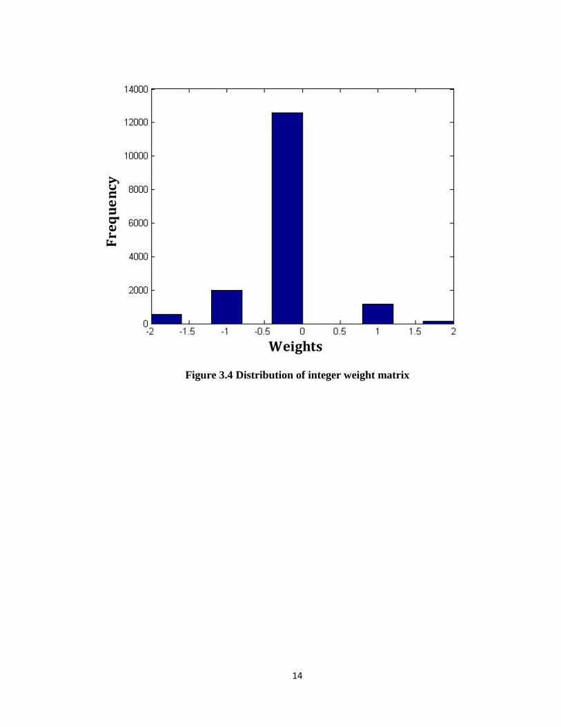
During training process, order of input images is random, hence the weights
obtained from every training process are different. Most of the times, it is observed that the
obtained weights are in the range [-4, 4]. We casted real valued weights in to integers in
order to map them to neuromorphic cores. Since our design is capable of storing multilevel
weights, we evaluated the robustness of the algorithm and circuit using different ranges of
the weight matrix such as [-3, 3], [-2, 2] and [-1, 1] which corresponds to 7 levels, 5 levels
and 3 levels respectively. Fig. 3.3 and fig. 3.4 shows distribution of weight matrix with real
number and integer format.
Fre
qu
en
cy
Weights
Figure 3.3 Distribution of real number weight matrix
14
Fre
qu
en
cy
Weights
Figure 3.4 Distribution of integer weight matrix

15
Chapter 4 Architecture and design
4.1 Neuronal dynamics
Axons, synapses and integrate and fire (I&F) neurons are the building blocks of our
neuromorphic core. Input signal coming from a previous neuron is communicated to next
neuron using a synapse. In order to overcome the bottle neck of Von Neumann
Architecture, we proposed the crossbar memory architecture as shown in figure 4.1.
Synapses and neurons are tightly integrated in order have faster access time. The
neuromorphic core contains K axons and N neurons. Axon j is connected to neuron i using
weight Wij. The magnitude of this weight defines strength of the connection between pre
and post synaptic neurons. Depending on value of weight, current is generated by a synapse
(Iij). Each neuron corresponds to two columns, one for excitatory and other for inhibitory
current. The current values on each column at a given time t is defined by the following
equation.
𝐼𝑖(𝑡) = ∑ 𝐴𝑗(𝑡)𝐾𝑗=1 ∗ 𝐼𝑖𝑗 (10)
Where Aj(t) is axonal input, which is defined by ith pixel of an image. Neuron compares
excitatory (Ii1) current against its inhibitory counterparts (Ii2) and generates a spike (Si)
depending on the threshold value θ. If the difference of excitatory and inhibitory current is
greater than threshold, neuron generates spikes as defined by equation (11).
𝑆𝑖(𝑡) = {1, 𝑖𝑓 (𝐼𝑖1 − 𝐼𝑖2) > 𝜃 0, 𝑜𝑡ℎ𝑒𝑟𝑤𝑖𝑠𝑒
(11)

16
MLC Array
E
Ax
on
cir
cuit
ry
I&F Neuron circuitry
Pixel-in
01….1
Spikes-out001..0
CntrlCkt
E
I
I
E
E
I
I
E
E
I
I
E
E
I
I
T T T T
E
I T
Excitatory cell
Inhibitory cell Threshold cell
Figure 4.1 Architecture of neuromorphic core
Each neuron has a threshold value. These threshold values are also programmed in
multilevel cells as shown in figure 4.1. Since threshold magnitude can be greater than a
maximum value that can be stored in a single cell, multiple cells of each column are used
to store a single value. The threshold value can either be positive or negative. Depending
on its polarity, it is either added to the excitatory current or inhibitory current. Positive
threshold is added to the inhibitory current and negative threshold is added to the excitatory
current.

17
4.2 Multicore design
In order to make the process of operation completely parallel, we took the
advantage of multicore design. As shown in figure 4.2, we used 4 core for this operation.
Each core has 64 axon and 64 neurons. Using 4 symmetric cores, our design demonstrates
a neuromorphic chip of 256 axons and 256 neurons. Since we use different columns for
excitatory and inhibitory synapses, the design constitutes 32K synapses.
RBM is trained with 256 input pixel images and 64 neurons which produces a
weight matrix of size 16K bits. Since each neuron processes excitatory and inhibitory
weights separately, we casted the 16K bit weights in to two matrices, one for excitatory
and one for inhibitory. Columns corresponding to each neuron are placed side by side for
fast access time. The adjacent placement of excitatory and inhibitory synapses would make
the design tolerant to process variations. On chip variation parameters such as Random
Dopant Fluctuation (RDF), temperature variations due to local hotspots are expected to
produce similar effect on both the columns and hence the neuronal spiking process is more
variation tolerant. 32K bit weights are divided in to 4 segment, horizontally. Each segment
of 8K bits is programmed in to one core.
Input image of 256 pixels is divided in to 4 segments of 64 pixels each. Each core
process 64 pixels and produces 64 corresponding spikes. These 4 neuromorphic cores
processes an entire image in a completely parallel fashion to produce 256 spikes, all
together. In order to take care of multicore design, we trained the off chip classifier with
spikes from all 4 cores together, using supervised learning. We designed the software
model to support different number of cores such as 1 core, 2 cores and 4 cores. It is
observed that the quality of classification is increased by increasing the number of cores.

18
Core 1
Core 2
Core 3
Core 4
Segment 1
Segment 2
Segment 3
Segment 4
64 Spikes
64 Spikes
64 Spikes
64 Spikes16x16 Pixel
image
Figure 4.2 Multicore design

19
4.3 Current based reading scheme
Most of the previous designs uses voltage based row-by-row reading scheme [2]-
[4]. Each pixel enables one word line and the synapses corresponding to the word line are
enabled. Then, the weights are read on to the bit lines and are accumulated at neurons. The
cycle continues until all the pixels corresponding to each image are processed. Once all the
weights are read, neurons compares the membrane potential with the threshold values and
generates spikes. The entire process from reading pixels to generating spikes takes time of
hundreds of clock cycles [14].
Another challenge of these conventional designs is the area overhead due to the
neuronal circuitry. As explained in [14] each neuron has a 10-bit adder, accumulator and
comparator. Design [4] would also require multiplier in order to process the grayscale
image directly. The area required by these conventional neuronal circuitry is very high.
We address both the challenges using our novel current based reading scheme as
shown in figure 4.3. Our reading scheme enables all the word lines together, hence current
on a bit line is sum of individual currents from all the synaptic cells in a column. Each
neuron has two currents, excitatory current (Iext) and inhibitory current (Iinh). Difference in
these two currents along with threshold current decides a spike. Since the process of
reading current is completely parallel, each neuron in all neuromorphic cores produces
spikes at same time. This makes reading operation very fast compared the conventional
row-by-row reading schemes. The area overhead of current based neurons is smaller than
the voltage based neuron circuits [4], [14]. Since all wordlines are enabled together, pixel
values of each image are stored on chip using scan flops.

20
E
E
E
T
I
I
I
T
Spike
+ -
WL<0>
WL<1>
WL<2>
WL<63>I ext
I inh
Current sensing neuron
E Excitatory cell
I Inhibitory cell
T Threshold cell
Figure 4.3 Current based reading scheme

21
4.4 Design floorplan
Figure 4.4 shows floor plan of the neuromorphic chip. In order to take advantage
of area, two cores are integrated together. Same design is replicated to make it a 4 core
design. Area of 2 cores is 1100x600 µm2. Eflash arrays corresponding to 2 cores are placed
together at the center to make the design denser. Sensing circuitry containing current based
neurons is placed below the array. Row decoder circuits and pixel-in scan cells are placed
on both the sides of the array. The corner blocks of the floor plan contains control circuitry
for memory and neuron operations.
The design contains 4 scan chains. Two for pixel-in data, one for programming
weights to core and one for reading out spikes. Initially, weights are programmed in to the
array. Later, neural operation is performed. The sequence of operation includes following
steps,
Loading pixel values in to the pixel-in scan chain serially.
Enabling wordlines corresponding to the active pixels.
Spike generation using neurons.
Loading spikes in to the spike-out scan chain.
Reading out spikes serially.
Once spikes corresponding to an image are read out, next image pixels are loaded in to the
pixel-in scan chain. Our design also includes redundant rows and columns in the array to
replace unexpected non-functional cells after fabrication.

22
1.1
mm
WL
D0
81
0x1
40
Cell array (68WLx320BL)
810x280
64WLs: EX/IN4WLs: Threshold
64 neurons/16 redun. neurons
Memory SCAN100x280
Pix
el-I
n S
CA
N0
81
0x2
0
Sensing circuit160x280
Spike-out SCAN30x280
WL
D1
81
0x1
40
Pix
el-I
n S
CA
N1
81
0x2
0
NeuronControl0
(with VREF)
NeuronControl1
Memory Control0
MemoryControl1
eFlash synapse: 1100x600μm2
600 μm
Figure 4.4 Chip floorplan

23
Chapter 5 Simulation results
Our neuromorphic circuit model designed in MATLAB can support various
configuration and sizes. The digit recognition accuracy is tested by changing different
parameters such as number of neurons, input image size, weight levels, number of cores
and introduced errors in the spikes. This section discusses accuracy trend of our software
model. For all different setups, the RBM and classifier are trained with 60,000 images and
are tested with other 10,000 images.
5.1 Accuracy trend with varying number of neurons
We studied digit recognition accuracy trend by varying number of neurons. All
input images used in the simulation are of size 484 pixels, weights are 9 levels [-4, 4]. A
single core design is considered for this study. Figure 5.1 shows accuracy trend. From the
graph it is observed that the accuracy of digit recognition decreases as the number of
neurons decrease. When the number of neurons is less than 64, the slope of the curve is
very high. However, as the number of neurons goes above 64, there is only slight gain in
the accuracy even with large increase in the number of neurons. As we can see, the
maximum accuracy is 92.7% when the number of neurons is 256. Even by increasing the
number of neurons beyond 256, the accuracy increase is negligible. The graph implies that
for the single core design, the accuracy of image recognition can still be maintained above
90% even after reducing the number of neurons to 64.

24
Figure 5.1 Digit recognition accuracy vs number of neurons
5.2 Accuracy as a function of image size
Size of the image plays a significant role in classification. Higher the number of
pixels, better is the image quality. Figure 5.2 shows images with different number of pixels.
As the number of pixels in the images decrease, the image quality drops significantly. By
fixing the number of neurons to 64 in a single core design, we have run the simulation with
different images of size 484, 256, 121, 64 and 25 pixels. Figure 5.3 shows dependency of
accuracy on size of the images. If the number of pixels are more than 121, digit recognition
accuracy doesn’t increase significantly with number of pixels. However, if the pixels are
less than 121, the size of an image has a significant impact on digit classification.
68.78
79.29
91.81 92.59 92.7
0
10
20
30
40
50
60
70
80
90
100
0 50 100 150 200 250 300
% A
ccu
racy
No. of Neurons
Digit recongition accuracy vs numberof neurons

25
22x22 pixels 16x16 pixels
11x11 pixels 8x8 pixels
Figure 5.2 Digits of different pixel sizes
Single core design with 64 neurons, 121 pixels and 9 level weights [-4, 4] would recognize
the images with 91% accuracy.

26
Figure 5.3 Digit recognition accuracy vs number of pixels
5.3 Impact of weight levels on accuracy
The advantage of multilevel memory cells over single bit memory is the array
density. Considering 64 neurons and 256 pixel images, we studied the impact of weight
levels on the digit classification. 4 configuration of weight levels are considered: 9 levels,
7 levels, 5 levels and 3 levels.
Since training process is random, depending on the weights matrix obtained every
cycle, image recognition accuracy varies. When the design is simulated for a same
configurations, it gives different accuracy value at each iteration. Figure 5.4 shows
accuracy values obtained out of 25 iterations. When we used 9 levels of weights, 8 out of
25 iterations gives accuracy above 80%. On the other hand, if we used 3 levels only 3
iterations gives accuracy above 80% as shown in figure 5.4.
77.25
88.13 90.99 91.52 91.81
0
10
20
30
40
50
60
70
80
90
100
0 100 200 300 400 500
% A
ccu
racy
Number of pixels
Digit recognition accuracy vs image size

27
80%
80%
% A
ccur
acy
% A
ccur
acy
Iterations
Iterations
Digit recognition accuracy for 9 level weights
Digit recognition accuracy for 3 level weights
Figure 5.4 Comparison of accuracies for different weight levels

28
Out of 25 cycles of simulations for each weight configuration, if we consider only
maximum accuracy, the obtained trend is shown in figure 5.5. Though weight levels have
a weaker dependency on maximum accuracy values, use of higher weight levels gives
higher digit recognition accuracy in most of the iterations.
Figure 5.5 Digit recognition accuracy vs weight levels
91.61 91.73 91.86 92.08
80
82
84
86
88
90
92
94
0 1 2 3 4 5 6 7 8 9 10
% A
ccu
racy
Weight levels
Maximum digit recognition accuracy vs weight levels

29
5.4 Grayscale vs binary pixel images
Impact of image type is one of the important studies in any image processing
application. We considered two types of image representations: grayscale and binary
images. In grayscale images, value of each pixel is represented on a scale from 0 to 255.
However, binary images have just two levels 0 or 255, as shown in figure 2.2 and figure
2.3. Digit recognition accuracy is weakly dependent on the number of levels in a pixel as
shown in figure 5.6. The figure compares digit recognition accuracies between grayscale
and binary images for 25 iterations. Each iteration is run with different set of weights. The
maximum accuracies with grayscale and binary images are 91.6% and 91.25%
respectively. The simulations are run considering 9 levels of weights and 64 neurons using
a single core design.
Figure 5.6 Digit recognition accuracy with grayscale and binary images
0102030405060708090
100
1 2 3 4 5 6 7 8 9 10 11 12 13 14 15 16 17 18 19 20 21 22 23 24 25
% A
CC
UR
AC
Y
ITERATIONS
Digit recognition accracy with different image types
Binary image Grayscale image

30
5.5 Accuracy trend with different number of cores
Studies from 5.1 to 5.4 are based on the single core design. However, if images are
very big, they have to be processed in segments. In order to demonstrate this idea, we
modeled multicores in our software. Each core processes 64 pixels and produces 64 spikes.
We segmented the weight matrix vertically and each segment is programmed in to a single
core. Each of these cores process the segments of images in parallel as shown in figure 4.2.
Considering 256 pixel images, 64 neurons for each core and 5 levels of weight, the
simulations are run for 1, 2 and 4 core designs. The accuracy of digit recognition is shown
in figure 5.7. Since 4 core structure gives highest accuracy, we designed our neuromorphic
chip with this configuration.
Figure 5.7 Digit recognition accuracy vs number of cores
91.73
93.7394.70
80
82
84
86
88
90
92
94
96
98
0 1 2 3 4 5
% A
ccu
racy
Number of cores
Digit recognition accuracy vs number of cores

31
5.6 Error tolerant design
Process of chip fabrication incur lot of variations in the circuits. This results in to
device mismatch. Even two similar circuits produce different current values for same bias
conditions. Since we are using current based neurons, there could be some errors in the
spikes. Considering the scenario, we modeled errors in spikes and observed digit
recognition accuracy. The accuracy is dropped by 12%, if we add 10% errors to spikes.
In order to address the issue, we trained our classifier in two phases. In first phase,
we train classifier with error free spikes corresponding to all 60,000 images. In second
phase, we introduced 10% errors in the spikes and trained the classifier again. Using this
training procedure, the accuracy has dropped by just 4-5% when 10% spike errors are
introduced in testing image. The trend is shown in figure 5.8. MATLAB simulations are
run on 4 core design with each core of size 64 axons and 64 neurons. Size of the images
used are 256 pixels and weight levels are 5.

32
Figure 5.8 Digit recognition accuracy vs spike errors

33
5.7 HSPICE simulation results
The functionality of neuromorphic core is verified using HSPICE simulations.
Since current based parallel reading scheme is used, better precision is required while
programming floating gate node voltages. Hence our circuit is designed to have flexibility
of verifying programmed weights in terms of drain current. Figure 5.9 shows simulation
results of internal current verification. Excitatory and inhibitory currents are compared with
reference current. Since we are verifying currents while programming weights, we can
program cells for same current even with different amount of variations in them. Even
though we encounter variations in eflash cells, current verification nullifies the effect.
Excitatory and inhibitory currents are verified separately. A neuron spikes when excitatory
current is greater than reference current during excitatory current verification. It also spikes
when inhibitory current is smaller than reference current during inhibitory current
verification.
COLMUX<1:0>
MODE<2:0>
CLK
EXC/INH
SA_EN
SPIKE
REF_CURRENT
EXC_CURRENT
INH_CURRENT
Excitatory current verification Inhibitory current verification
EX > REF REF > IN
Process: ST 65nm Voltage: 1.2V Temp.: 25°C
Figure 5.9 Internal current verification

34
Once the programmed weights are verified, neuron operation is performed. During
this mode, all the wordlines corresponding to pixel value “high” are enabled. Eflash cells
connected to these wordlines start conducting current. The magnitude of bitline current
depends on programmed weights at each cell. Neuron compares excitatory and inhibitory
currents to generate spikes. Spikes are generated if excitatory current is larger than
inhibitory current as shown in figure 5.10.
The simulation involves initializing hundreds of floating gate node voltages,
enabling wordlines depending on the values of pixels and reading out spikes. The entire
process is automated using PERL scripting. Spikes of software simulations are compared
with spikes of hardware simulations to verify the functionality of the design.
COLMUX<1:0>
MODE<2:0>
Erase mode Program mode Neuron sensing mode
CLK
WWLRWL/EWL
PWLFloating gate node
SA_EN
Excitatory current
Inhibitory current
SPIKE
Process: ST 65nm Voltage: 1.2V Temp.: 25°C
Figure 5.10 Neuron operation

35
Although process variation at eflash cells is nullified by using internal current
verification, there could be some variations at neurons. This variation causes an offset
current at neuron. Anticipating this issue, we modelled Gaussian distribution of offset
current at neurons as shown in figure 5.11. Since these variations are permanent and
localized to each neuron, training the classifier with these effects could still recognize the
digits with 94.7% accuracy. Neurons are also designed to have optional offset currents to
overcome these issues.
-4 -3 -2 -1 0 1 2 3 4 0
2
4
6
8
10
12
Fre
qu
en
cy
Offset current (µA)
Gaussian distribution of variation(offset current)
Offset current range(-0.5µA to 0.5µA)
Figure 5.11 Gaussian distribution of offset current
Since eflash uses charge to store the weight levels, it could experience charge loss
due to gate leakage. However, the effect is expected to be even on the adjacent columns,
which are used for current comparison. This makes the design robust to retention related
issues.
36
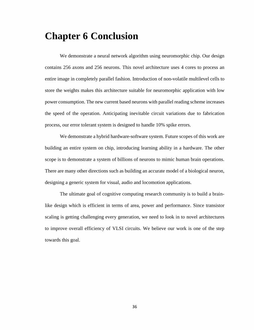
Chapter 6 Conclusion
We demonstrate a neural network algorithm using neuromorphic chip. Our design
contains 256 axons and 256 neurons. This novel architecture uses 4 cores to process an
entire image in completely parallel fashion. Introduction of non-volatile multilevel cells to
store the weights makes this architecture suitable for neuromorphic application with low
power consumption. The new current based neurons with parallel reading scheme increases
the speed of the operation. Anticipating inevitable circuit variations due to fabrication
process, our error tolerant system is designed to handle 10% spike errors.
We demonstrate a hybrid hardware-software system. Future scopes of this work are
building an entire system on chip, introducing learning ability in a hardware. The other
scope is to demonstrate a system of billions of neurons to mimic human brain operations.
There are many other directions such as building an accurate model of a biological neuron,
designing a generic system for visual, audio and locomotion applications.
The ultimate goal of cognitive computing research community is to build a brain-
like design which is efficient in terms of area, power and performance. Since transistor
scaling is getting challenging every generation, we need to look in to novel architectures
to improve overall efficiency of VLSI circuits. We believe our work is one of the step
towards this goal.

37
Bibliography
[1] R. Ananthanarayanan, et al., “The cat is out of the bag: cortical simulations with
109 neurons, 1013 synapses,” Proc. Conf. High Perf. Computing Networking,
Storage and Analysis (SC09), pp. 1-12, Nov. 2009.
[2] J. Seo, et al., “A 45nm CMOS Neuromorphic Chip with a Scalable Architecture for
Learning in Networks of Spiking Neurons,” Proc. IEEE Custom Integrated Circuits
Conference, 2011.
[3] P. Merolla, J. Arthur, F. Akopyan, N. Imam, R. Manohar, and D. S. Modha, “A
digital neurosynaptic core using embedded crossbar memory with 45 pJ per spike
in 45 nm,” Proc. IEEE Custom Integr. Circuits Conf., 2011.
[4] P. Knag, J. Kim, T. Chen, Z. Zhang, “Sparse Coding Neural Network ASIC With
On-Chip Learning for Feature Extraction and Encoding,” IEEE Journal of Solid-
State Circuits, Vol. 50, No. 4, April 2015.
[5] S. Moradi, G. Indiveri, “A VLSI network of spiking neurons with an asynchronous
static random access memory,” IEEE Biomedical Circuits and Systems Conference
(BioCAS), 2011.
[6] M. Suri, et al., “CBRAM devices as binary synapses for low-power stochastic
neuromorphic systems: Auditory (Cochlea) and visual (Retina) cognitive
processing applications,” IEEE Intl. Electron Devices Meeting (IEDM), 2012.
[7] S. Park, et al., “Neuromorphic speech systems using advanced ReRAM-based
synapse,” IEEE Intl. Electron Devices Meeting (IEDM), 2013.

38
[8] G. Indiveri, E. Chicca, and R. Douglas, “A VLSI array of low-power spiking
neurons and bistable synapses with spike-timing dependent plasticity,” IEEE
Trans. Neural Networks, Feb. 2006.
[9] C. Bartolozzi, G. Indiveri, “Synaptic Dynamics in Analog VLSI,” Neural
Computation, Vol. 19, Oct. 2007.
[10] S. Song, K. C. Chun, C.H. Kim, “A Logic-Compatible Embedded Flash Memory
for Zero-Standby Power System-on-Chips Featuring a Multi-Story High Voltage
Switch and a Selective Refresh Scheme,” IEEE Journal of Solid-State circuits, May
2013.
[11] S. Song, K. C. Chun, C.H. Kim, “A Bit-by-Bit Re-Writable Eflash in a Generic 65
nm Logic Process for Moderate-Density Nonvolatile Memory Applications,” IEEE
Journal of Solid-State circuits, Aug. 2013.
[12] A. Steiner, et al., “1kHz 2D silicon retina motion sensor platform,” IEEE Intl.
Symposium on Circuits and Systems (ISCAS), 2014.
[13] C. Brandli, et al., “A 240 × 180 130 dB 3 µs Latency Global Shutter Spatiotemporal
Vision Sensor,” IEEE Journal of Solid-State circuits, Sept. 2014.
[14] N. Iman, et al., “A Digital Neurosynaptic Core Using Event-Driven QDI Circuits,”
IEEE Intl. Symposium on Asynchronous Circuits and Systems (ASYNC), 2012.
[15] F. Tenore et al., “A spiking silicon central pattern generator with floating gate
synapses,” IEEE Intl. Symposium on Circuits and Systems, 2005.
[16] E. Painkras, et al., “Spinnaker: A 1-w 18-core system-on-chip for massively-
parallel neural network simulation,” IEEE Journal of Solid-State Circuits, 2013.

39
[17] B.V. Benjamin, et al., “Neurogrid: A Mixed-Analog-Digital Multichip System for
Large-Scale Neural Simulations,” proceedings of the IEEE, April 2014.
[18] G. E. Hinton and R. R. Salakhutdinov, “Reducing the dimensionality of data with
neural networks,” Science, vol. 313, no. 5786, pp. 504–507, July 2006. Online
available: http://dx.doi.org/10.1126/science.1127647.
[19] The MNIST dataset is available at http://yann.lecun.com/exdb/mnist/index.html
[20] G.E. Hinton and S. Osindero, “A fast learing algorithm for deep belief nets,” Neural
Computation, Vol. 19, July 2006.