MNRAS 480, 2743–2756 (2018) doi:10.1093/mnras/sty1960Advance Access publication 2018 July 23

A multifrequency radio continuum study of the Magellanic Clouds – I.Overall structure and star formation rates

B.-Q. For,1,2 L. Staveley-Smith,1,3 N. Hurley-Walker,4 T. Franzen,4

A. D. Kapinska,1,3,5 M. D. Filipovic,6 J. D. Collier,6,7,8 C. Wu,1 K. Grieve,6

J. R. Callingham,9 M. E. Bell,3,10 G. Bernardi,11 J. D. Bowman,12 F. Briggs,13

R. J. Cappallo,14 A. A. Deshpande,15 K. S. Dwarakanath,15 B. M. Gaensler,3,16,17

L. J. Greenhill,18 P. Hancock,3,4 B. J. Hazelton,19 L. Hindson,20 M. Johnston-Hollitt,4,21

D. L. Kaplan,22 E. Lenc,3,17 C. J. Lonsdale,14 B. McKinley,3,23 S. R. McWhirter,14

D. A. Mitchell,3,7 M. F. Morales,19 E. Morgan,24 J. Morgan,4 D. Oberoi,25 A. Offringa,7

S. M. Ord,3,7 T. Prabu,15 P. Procopio,23 N. Udaya Shankar,15 K. S. Srivani,15

R. Subrahmanyan,3,15 S. J. Tingay,3,4 R. B. Wayth,3,4 R. L. Webster,3,23 A. Williams,4

C. L. Williams24 and Q. Zheng26

Affiliations are listed at the end of the paper

Accepted 2018 July 15. Received 2018 June 27; in original form 2018 January 7

ABSTRACTWe present the first low-frequency Murchison Widefield Array (MWA) radio continuum mapsof the Magellanic Clouds (MCs), using mosaics from the GaLactic Extragalactic All-Sky MWA(GLEAM) survey. In this paper, we discuss the overall radio continuum morphology between76 and 227 MHz and compare them with neutral hydrogen maps, 1.4 GHz continuum maps andoptical images. Variation of diffuse emission is noticeable across the Large Magellanic Cloud(LMC) but absent across the bar of the Small Magellanic Cloud (SMC). We also measurethe integrated flux densities and derive the spectral indices for the MCs. A double power-lawmodel with fixed α1 = −0.1 fit between 19.7 MHz and 8.55 GHz yields α0 = −0.66 ± 0.08for the LMC. A power-law model yields α85.5MHz

8.55GHz = −0.82 ± 0.03 for the SMC. The radiospectral index maps reveal distinctive flat and steep spectral indices for the H II regions andsupernova remnants, respectively. We find strong correlation between H II regions and Hα

emission. Using a new 150 MHz–Hα relation as a star formation rate indicator, we estimateglobal star formation rates of 0.068–0.161 M� yr−1 and 0.021–0.050 M� yr−1 for the LMCand SMC, respectively. Images in 20 frequency bands, and wideband averages are madeavailable via the GLEAM virtual observatory server.

Key words: radiation mechanisms: non-thermal – radiation mechanisms: thermal –Magellanic Clouds – radio continuum: galaxies.

1 IN T RO D U C T I O N

The Large and Small Magellanic Clouds (LMC and SMC) lie ata distance of about 50 and 60 kpc (Hilditch, Howarth & Harries2005; Pietrzynski et al. 2013), respectively, and are among the clos-est extragalactic neighbours of our Galaxy. The close proximity ofthe Magellanic Clouds (MCs) provides an ideal laboratory for us

� E-mail: biqing.for@uwa.edu.au

to probe different physical mechanisms in great detail. Pioneeringstudies of the MCs in radio continuum emission date back to the1950s (see e.g. Mills 1955; Shain 1959). Subsequent studies havebeen carried out to either focus on individual objects (e.g. supernova1987A; Zanardo et al. 2010 and references therein) or large-scaleradio structure and total radio spectrum of the MCs (Haynes et al.1991 and references therein; Hughes et al. 2007). Aside from ra-dio continuum studies, there have been many other comprehensivemultiwavelength studies to date (see e.g. Jameson et al. 2016). Yet,there is more to learn about these nearby galaxies.

C© 2018 The Author(s)Published by Oxford University Press on behalf of the Royal Astronomical Society

Downloaded from https://academic.oup.com/mnras/article-abstract/480/2/2743/5057489by Univ Western Australia useron 04 September 2018

2744 B.-Q. For et al.

Radio continuum studies probe two main astrophysical proper-ties: non-thermal synchrotron emission that is generated by rela-tivistic charged particles accelerated in magnetic fields; and ther-mal free–free emission from ionized hydrogen clouds (HII regions;Lisenfeld & Volk 2000). The former partly originates from dis-crete supernova remnants (SNRs). However, studies have shownthat only about 10 per cent of the non-thermal synchrotron emis-sion is originated from SNRs (Lisenfeld & Volk 2000) and about90 per cent probably due to the propagation of cosmic ray electronsthroughout the galaxy disc (Condon 1992) over time-scales of 10to 100 Myr (Helou & Bicay 1993). The origin of these electronsis unknown, but could mostly still be from SNRs and supernovaexplosions. Free–free emission originates from the thermal ionizedgas in general including the diffuse ionized gas, though it is strongerin HII regions. Since massive stars (M > 8 M�) have a relativelyshort lifetime (<108 yr), this emission therefore traces recent starformation activity.

The intensity of thermal free–free emission is directly propor-tional to the total number of Lyman continuum photons. In theoptically thin regime, the spectrum of a galaxy can generally bedescribed by a power-law function, Sν∝να , where Sν is the radioflux density at a given frequency, ν, and α is the spectral index (orpower-law slope). The spectrum is “flat” when α ∼ −0.1. Steepspectra with α ∼ −0.8 are commonly observed in star-forminggalaxies (see Marvil, Owen & Eilek 2015 and references therein).Low-frequency turn-over occurs when the optical depth changesfrom optically thin to optically thick due to absorption process.

With new state-of-the art low-frequency telescopes, such as theMurchison Widefield Array (MWA; Lonsdale et al. 2009; Bow-man et al. 2013; Tingay et al. 2013), it is feasible to carry out newcontinuum surveys with fast survey speeds to probe astrophysicalprocesses at these frequencies. In this paper, we present a multifre-quency study of the MCs using data from the GaLactic ExtragalacticAll-sky MWA (GLEAM) survey (Wayth et al. 2015; Hurley-Walkeret al. 2017), the Parkes single-dish radio telescope and radio interfer-ometer data from the Australia Telescope Compact Array (ATCA).In Section 2, we describe the GLEAM observations and data reduc-tion. We show the radio continuum maps of the MCs and discusstheir morphology in comparison with the integrated neutral hydro-gen (H I) maps and optical images in Section 3. Our analysis andresults are presented in Section 4. In Section 5, we derive the globalstar formation rates. Our investigation of spatial variation of thespectral index among H II regions, a possible turn-over frequencyand the production rates of Lyman continuum photons is describedin Section 6. Lastly, we present our conclusions and outlook inSection 7.

2 O B S E RVAT I O N S A N D DATA R E D U C T I O N

The MWA is a low-frequency radio interferometer operating be-tween 70 and 300 MHz. It was designed to have a wide field ofview (15◦–50◦) and a short-medium baseline distance suitable fordetecting the faint redshifted 21-cm spectral line emission from theEpoch of Reionization (EoR), as well as supporting a wide rangeof other astrophysics applications (Bowman et al. 2013). Phase 1 ofMWA consisted of 128 32-dipole antenna tiles that spread acrossan area of ∼3 km in diameter. We refer the reader to Tingay et al.(2013) for technical details.

The GaLactic Extragalactic All-sky MWA (GLEAM) survey isthe main MWA continuum survey that covers the sky south of dec-lination +30◦ with a frequency range of 72–231 MHz split into fiveseparated sub-bands (Wayth et al. 2015). The data were collected

in nightly drift scans, where all frequencies for a single declinationstrip were observed each night. The data reduction process is de-scribed in detailed in Wayth et al. (2015) and Hurley-Walker et al.(2017). To summarize, raw visibility data were processed usingCOTTER (Offringa et al. 2015), which performs flagging and aver-aging of the visibility data to a time resolution of 4 s and a frequencyresolution of 40 kHz. Subsequent calibration involved the creationof a sky model for each observation, “peeling” to minimize sidelobesfrom the bright sources, and astrometric correction for ionosphericeffects. Lastly, a single mosaic per sub-band is obtained by combin-ing all declination strips from each week of observations. A slightapparent blurring of the point spread function (PSF) is noted due toslightly different ionospheric conditions in the 20–40 observationsper pixel. To take this into account, PSF maps are created for eachmosaic as a function of position on the sky, with three channelswhose pixels represented the major axis, minor axis, and positionangle.

We employ the final flux calibrated mosaic imaged with robustweighting of 0 (Briggs 1995) for this study because the theoreti-cal noise is lower than standard GLEAM data reduction, and thebrightness sensitivity is higher. Uncertainty in the flux density scalemainly arises from the declination-dependent flux density correc-tion. The systematic uncertainty (σ scale) is derived as the standarddeviation of a Gaussian fit to the residual variation in the ratio of pre-dicted to measured source flux densities. The systematic uncertain-ties for the studied regions are 8.5 per cent (LMC) and 13 per cent(SMC) (Hurley-Walker et al. 2017).

3 R A D I O C O N T I N U U M M A P S O F T H EM AG E L L A N I C C L O U D S

We present a series of selected GLEAM images of the MCs inFig. 1. Due to varying PSF across the large area of the MCs images,we derive the synthesized beam sizes by averaging the values of thecorresponding PSF map of each band for the analysed area. The typ-ical PSF variation across each field is 15–20 per cent. A summaryof the observed central frequency, synthesized beam, pixel area, andaverage noise level (RMS) for the 20 GLEAM sub-bands imagesis given in Table 1. We present combined three colour compositeimages of the LMC and SMC in Fig. 2. Optically thick H II regionsappear to be bluer due to their positive steep spectral index (α ∼ 2;Condon 1992).

The overall radio continuum morphology of the LMC shows adistinct asymmetry, with the eastern side being brighter and com-pressed. This asymmetry is also visible in the combined single-dish(Parkes) and interferometer (ATCA) H I map (Kim et al. 2003;Staveley-Smith et al. 2003) as shown by the contours in Fig. 3. Wenote that the compressed side of the LMC is facing the direction ofproper motion of the LMC (Kallivayalil et al. 2013; van der Marel& Kallivayalil 2014) and leading the trailing Magellanic Stream.The “arm” structures as seen in the H I map, as well as the 1.4 GHz(Feitzinger et al. 1987) and 4.75 GHz (Haynes et al. 1991) radiocontinuum maps, are also visible in the MWA images.

The most notable concentration of radio continuum emission isat the largest H II region, 30 Doradus, where the H I column densityis high enough to fuel star formation. The lesser explored star-forming complex, N79, in the south-west region of the LMC hasrecently been reported to possess more than twice the star formationefficiency of 30 Doradus (Ochsendorf et al. 2017). Interestingly, forboth N11 and N79 which are among the largest star-forming regionsin the LMC, the radio continuum is relatively weak in all GLEAMsub-bands. Other patches of strong emission are also consistent

MNRAS 480, 2743–2756 (2018)Downloaded from https://academic.oup.com/mnras/article-abstract/480/2/2743/5057489by Univ Western Australia useron 04 September 2018

A radio continuum study of the MCs 2745

Figure 1. Selected radio images of the LMC and SMC from the GLEAM survey. From top left to bottom right are images centred at 92, 115, 143, 166, 189,and 212 MHz. The grey scale is in units of Jy beam−1.

MNRAS 480, 2743–2756 (2018)Downloaded from https://academic.oup.com/mnras/article-abstract/480/2/2743/5057489by Univ Western Australia useron 04 September 2018

2746 B.-Q. For et al.

Table 1. Basic information for the GLEAM images in this study. ν represents the central frequency of the observed sub-band. σ is the average rms of threeselected emission free regions. Synthesized beams are derived from the associated PSF map (Section 2).

ν FWHMLMC FWHMSMC Pixel Size σLMC σ SMC

(MHz) (arcsec) (arcsec) (arcsec) (Jy beam−1) (Jy beam−1)

76 471.5 × 411.6 495.4 × 455.6 61.2 0.092 0.07984 423.5 × 370.5 443.0 × 410.2 61.2 0.056 0.05992 390.4 × 343.1 407.2 × 378.2 61.2 0.056 0.06399 367.6 × 319.6 380.4 × 353.9 61.2 0.068 0.055107 334.5 × 294.5 356.8 × 333.0 45.4 0.041 0.041115 307.3 × 272.5 328.0 × 306.4 45.4 0.036 0.036123 289.3 × 256.8 309.8 × 288.2 45.4 0.029 0.032130 279.6 × 246.6 293.4 × 276.2 45.4 0.030 0.032143 255.2 × 220.9 271.8 × 255.9 34.9 0.022 0.029150 240.0 × 208.3 254.4 × 239.5 34.9 0.020 0.025158 229.3 × 198.8 242.6 × 229.3 34.9 0.019 0.026166 220.4 × 190.8 234.5 × 222.6 34.9 0.018 0.024174 212.6 × 184.7 224.5 × 212.6 29.1 0.020 0.025181 202.4 × 177.2 214.4 × 203.4 29.1 0.018 0.021189 193.4 × 168.6 208.1 × 196.4 29.1 0.020 0.021197 188.1 × 163.9 202.1 × 189.4 29.1 0.019 0.020204 182.0 × 157.9 197.2 × 184.5 25.0 0.018 0.019212 173.4 × 150.9 189.2 × 176.6 25.0 0.017 0.019219 169.5 × 147.0 183.4 × 170.4 25.0 0.018 0.019227 164.8 × 142.9 178.9 × 165.6 25.0 0.017 0.019

Figure 2. Three colour RGB composite images of the Magellanic Clouds using the combination of 123, 181, and 227 MHz images, respectively. Images arereprojected and regridded to a common projection and angular resolution of 123 MHz images prior to combination. Left: Large Magellanic Cloud in a 10◦×10◦ image, Right: Small Magellanic Cloud in a 6◦× 6◦ image.

with supershell locations, where the shell interaction and expansioncould also be triggering star formation.

An asymmetry is also seen in deep optical images of the LMC(Besla et al. 2016), except that the overdensity of the stellar com-ponent is located at the opposite side (west) of the radio continuumemission. Since the old stellar population results in this overden-sity on the western side of the LMC, detection of radio continuumemission is not expected. The asymmetric feature as shown in both

radio and optical has been studied in simulations and concluded tobe evidence of tidal interaction between our Milky Way and theMCs and a result of ram-pressure (see Diaz & Bekki 2011; Beslaet al. 2016; Mackey et al. 2016).

Fig. 3 (bottom panel) shows the 227 MHz radio continuum imageof the SMC overlaid with HI contours (Stanimirovic et al. 1999).The overall morphology of the SMC’s radio continuum emissionis similar to H I, its stellar distribution, and with the dominant of

MNRAS 480, 2743–2756 (2018)Downloaded from https://academic.oup.com/mnras/article-abstract/480/2/2743/5057489by Univ Western Australia useron 04 September 2018

A radio continuum study of the MCs 2747

Bar

Wing

N83/N84

Figure 3. Top: H I column density contours (Kim et al. 2003; Staveley-Smith et al. 2003) at 2 × 1021 cm−2 (brown) and 4 × 1021 cm−2 (green) areoverlaid on to the 227 MHz GLEAM radio continuum map of the LMC. TheHI map is convolved and regridded to match the resolution and pixel scaleof the 227 MHz GLEAM image. The grey scale is in units of Jy beam−1.The directions of proper motion and the Magellanic Stream are indicatedby arrows. Extended H I and radio continuum emission south of 30 Doraduspoint toward the Magellanic bridge and the SMC. Bottom: As top, with theaddition H I column density contour level at 6 × 1021 cm−2 for the SMC(Stanimirovic et al. 1999). The bar and wing are labelled.

bright H II complexes across the bar. There is visible diffuse emissionextending out from the bar region toward the south-east side (SMCwing) and the H II complexes (N83/84; Bolatto et al. 2003). Thefurther extensions known as the SMC “tail” (Stanimirovic et al.1999) and Magellanic bridge (Bruns et al. 2005) are quite distinctin H I. A stellar component has been found in the bridge suggestingstripped material due to tidal interaction (Harris 2007) but the youngstellar component also suggests ongoing star formation (Chen et al.2014).

4 A NA LY SI S AND RESULTS

4.1 Integrated flux densities

To obtain the spatially integrated flux densities (Sν), we extract 8◦ ×8◦ and 6◦ × 6◦ images centred on the LMC and SMC, respectively,from the mosaic in each band. Subsequently, we mask out pixelsbelow 3σ background noise level of the extracted GLEAM images.The background noise level (σ RMS) is the average of measuredvalues of three selected emission-free regions around the MCs. Thesame regions are used for all bands. The Sν is then calculated using

Sν = Sνtotal × p2

1.133 θa θb

, (1)

where Sνtotal is the total flux density (Jy) of the 8◦× 8◦ (LMC) or 6◦×6◦ (SMC) image, p is the pixel size, θa and θb are the full-width-half-maximum (FWHM) of the telescope beam’s major and minoraxis (refer Table 1). We also measure Sν from archival 1.4 GHz(Hughes et al. 2007) and 4.8 GHz (Haynes et al. 1991) images ofthe LMC. As for the SMC, archival 1.4 GHz (Staveley-Smith et al.1997) and 2.37 GHz (Filipovic et al. 2002) images are also used fordetermining Sν . The same integration areas as those applied to theGLEAM images are used to determine Sν for the archival data. The4.8 GHz LMC image and 2.37 GHz SMC image were observed bythe single-dish Parkes 64-m telescope. Both 1.4 GHz images of theLMC and SMC are combined single-dish and interferometer data.All measurements are brought to the same absolute flux densityscale of Baars et al. (1977).

The errors for the measured integrated flux density are determinedusing

σtotal =√

(σimage)2 + (σscale)2, (2)

where σ image is equal to σRMS × √N , N is the integrated area in units

of the synthesized beam area, and σ scale is the systematic uncertaintyin the flux scale (see Section 2).

Tables 2–3 summarize our measurements and values obtainedfrom the literature at other frequencies. We note that flux densitiesat 85.5 and 96.8 MHz in Mills (1959) revised by Klein et al. (1989)are significantly higher than our measurements despite these valueshave been scaled to match the flux density scale of Baars et al. (1977)and corrected for unrelated foreground and background sources.Despite this discrepancy, we still include 85.5 and 96.8 MHz valuesin our spectral fitting.

The LMC is located in a region of sky in which the Galacticforeground emission is negligible at MHz and GHz frequencies.However, extended Galactic foreground emission is known to bepresent at the location of the SMC (see discussion in Haynes et al.1991 and references therein). Examining the SMC region in the408 MHz all-sky survey of (Haslam et al. 1981), we find that thestrongest Galactic foreground emission is located beyond the 6◦×6◦ region that we use in this study. Measurements of Haynes et al.(1991) have taken into account for the extended Galactic foregroundemission because of the larger imaging area than ours. Their stud-ies were conducted using a single-dish telescope. With the use ofinterferometer data from the MWA, it is possible to resolve out fluxfrom large-scale structure. Based on the shortest baseline of phase IMWA (7.7 m), the largest angular scales for 76 MHz and 227 MHzare 29◦ and 10◦, respectively. Since these angular scales are largerthan our studied regions, we do not expect our measurements to beaffected by missing flux in the GLEAM images.

MNRAS 480, 2743–2756 (2018)Downloaded from https://academic.oup.com/mnras/article-abstract/480/2/2743/5057489by Univ Western Australia useron 04 September 2018

2748 B.-Q. For et al.

Table 2. Integrated flux densities (Sν ) of the Large Magellanic Cloud.

ν Sν σ Reference(MHz) (Jy) (Jy)

19.7 5270 1054 Shain (1959)a

45 2997 450 Alvarez, Aparici & May (1987)85.5 3689 400 Mills (1959)a

96.8 2839 600 Mills (1959)a

158 1736 490 Mills (1959)a

76 1855.3 315.6 This study84 1775.7 302.0 This study92 1574.9 267.9 This study99 1451.6 247.0 This study107 1827.6 310.8 This study115 1627.5 276.8 This study123 1643.3 279.4 This study130 1571.8 267.3 This study143 1663.7 282.9 This study150 1450.1 246.6 This study158 1350.4 229.6 This study166 1204.3 204.8 This study174 1341.4 228.1 This study181 1247.1 212.1 This study189 1223.9 208.1 This study197 1109.8 188.8 This study204 1235.3 210.1 This study212 1121.6 190.8 This study219 1032.4 175.6 This study227 1019.7 173.4 This study408 925 30 Klein et al. (1989)1400 384 30 This studyb

1400 529 30 Klein et al. (1989)2300 412 50 Mountfort et al. (1987)2450 390 20 Haynes et al. (1991)4750 363 30 Haynes et al. (1991)4750 300 40 This studyc

8550 270 35 Haynes et al. (1991)

Notes. aValues revised by Klein et al. (1989).bUsing image from Hughes et al. (2007).cUsing image from Haynes et al. (1991).

4.2 SED modelling

The radio spectrum of a galaxy can normally be approximated bya power-law function, whose slope depends on the thermal andnon-thermal nature of the emission. At low-radio frequencies, thespectrum can turn over due to several absorption mechanisms. In thecase of the MCs, where there is no evidence of a turn-over, modellingof spectral energy distribution (SED) can take the general forms asdescribed below. We fit the SEDs of the MCs with (a) a power lawor (b) a curved power law, or (c) a double power law. A power lawis defined as

Sν = S0

(ν

ν0

)α

, (3)

or in logarithmic form as

log10(Sν) = log10(S0) + α log10

(ν

ν0

), (4)

where ν0 is the reference frequency, S0 is the flux density at thereference frequency, and α is the spectral index. A curved powerlaw extends the power law to a quadratic function in logarithmicform that allows for a curvature parameter, c,

log10(Sν) = log10(S0) + α log10

(ν

ν0

)+ c log10

(ν

ν0

)2

. (5)

Table 3. Integrated flux densities (Sν ) of the Small Magellanic Cloud.

ν Sν σ Reference(MHz) (Jy) (Jy)

85.5 460 200 Mills (1955, 1959)a

76 403.9 105.2 This study84 291.4 76.0 This study92 249.8 65.3 This study99 262.2 68.5 This study107 354.4 92.3 This study115 270.5 70.5 This study123 257.3 67.0 This study130 244.1 63.6 This study143 324.6 84.5 This study150 258.3 67.3 This study158 264.1 68.8 This study166 217.1 56.6 This study174 356.6 92.8 This study181 282.8 73.6 This study189 250.4 65.2 This study197 246.8 64.3 This study204 291.4 75.9 This study212 230.7 60.1 This study219 219.5 57.2 This study227 215.2 56.1 This study408 133 10 Loiseau et al. (1987)1400 42 6 Loiseau et al. (1987)b

1400 34.7 2.0 This studyc

2300 31 6 Mountfort et al. (1987)2300 27.1 7.0 This studyd

2450 26 3 Haynes et al. (1991)4750 19 4 Haynes et al. (1991)8550 15 4 Haynes et al. (1991)

Notes. aValues revised by Loiseau et al. (1987).bValues revised by Haynes et al. (1991).cUsing image from Staveley-Smith et al. (1997).dUsing image from Filipovic et al. (2002).

To take into account any “flattening” of the spectrum, we canfit the spectrum with a double power-law model, with the firstand second component identified by subscripts 0 and 1. These twocomponents generally represent the synchroton (non-thermal) andfree–free (thermal) spectral indices. The model is defined as

Stot = S0

(ν

ν0

)α0

+ S1

(ν

ν0

)α1

. (6)

In the optically thin regime, thermal free–free emission from ther-mal electrons is often characterized by α = −0.1 (Klein et al. 1989).We fit the spectra by allowing α0 and α1 as free parameters and alsoby setting a fixed α1 = −0.1 (thermal). A reference frequency of200 MHz is used throughout the modelling. We also adopt non-linear least squares Lavenberg–Marquardt algorithm for the fitting.We found it necessary to scale the MWA errors by a factor of two toprevent the MWA data points from dominating the overall fit. Werefer readers to Harvey et al. (2018) for a detailed description andcaveats on SED modelling.

4.2.1 Model selection

To select the best model, we first calculate the χ2red, given by

χ2red = χ2

dof= χ2

N − k, (7)

MNRAS 480, 2743–2756 (2018)Downloaded from https://academic.oup.com/mnras/article-abstract/480/2/2743/5057489by Univ Western Australia useron 04 September 2018

A radio continuum study of the MCs 2749

where dof is the degree of freedom, N is the number of data points,and k is the number of fitted parameters. We also calculate theBayesian Information Criterion (BIC; Schwarz 1978), which is de-fined as

BIC = k ln(N ) − 2 ln L, (8)

L =N∏

i=1

1

σi

√2π

exp

(− 1

2σ 2i

(Sνi− f (νi))

2

), (9)

where L is the likelihood function, k and N are the same parametersas in equation (7), Sνi

and σ i are flux density and uncertainty atfrequency ν, respectively. For comparing the two models, a BIC= BICm1 −BICm2 is calculated. If BIC is positive, it is in favourof model 2. The model with the lowest BIC is preferred and BICneeds to be > 2 to be statistical significant (Kass & Raftery 1995).Our sequence of comparison starts from the first model and itera-tively moves to the next model.

Based on the BIC values, we find the preferred model to be thedouble power law with fixed α1 = −0.1 (model 3) for the LMC. Thismodel yields α0 = −0.66 ± 0.08 (non-thermal). This suggests thatsynchrotron radiation dominates at lower frequencies and thermalfree–free emission takes over at higher frequencies. For the SMC,BIC values of model 2–4 are negative which implies the powerlaw (model 1) is the preferred model. A summary of the SED fittingresults and associated statistical values is given in Table 4. Fig. 4shows the best fitting models for the LMC and SMC, respectively.

4.2.2 Comparison with previous studies

The derived non-thermal spectral index (α0 = −0.66 ± 0.08) be-tween 19.7 MHz and 408 MHz, for the LMC is consistent with Kleinet al. (1989), α19.7 MHz

2.3 GHz =−0.70 ± 0.06. For the SMC, we deriveα85.5 MHz

8.55 GHz = −0.82 ± 0.03, which is also consistent with the litera-ture value of α85.5 MHz

8.55 GHz =−0.85 ± 0.05 (Haynes et al. 1991). Com-paring our derived spectral index of the SMC to the mean spectralindex derived from all sources in the SMC (αSMC = −0.73 ± 0.05;Filipovic et al. 1998), we do not find significant differences.

4.3 Intensity variation across the MCs

In Section 3, we show that the LMC exhibits an asymmetric mor-phology in the radio continuum map. We examine the intensityvariation across the LMC in 10 MWA frequency bands (see Fig. 5).By dissecting the disc of the LMC through the 30 Doradus region,we find that there are a few peaks associated with the HII regionsand supernova remnants. The diffuse emission exhibits constant in-tensity on the eastern side. A gradual decline in intensity from rightascension ∼5h16m48s onward to the western end is noticeable. Inthe north–south direction, the intensity of diffuse emission declineswhen moving away from the 30 Doradus region. A steeper declineof intensity south of 30 Doradus is seen as compared to the northernpart. Compared with the 1.4 GHz radio continuum intensity profilesas shown in fig. 7 of Hughes et al. (2007), the north–south intensityprofile is quite similar. We examined the intensity profiles acrossthe bar and north–south direction of the SMC (not shown here),which show that there is no variation apart from a few intensitypeaks contributed by the HII regions.

4.4 Contribution from background radio sources

The areas we use for measuring the total flux densities of the MCsinclude background radio sources. The contribution from the back-

Table 4. A summary of the fits to the SED of the MCs using four differentmodels discussed in the text. The reference frequency is 0.2 GHz.

LMC SMC

Power lawModel 1

χ2 61.5 32.3χ2

red 2.0 1.2BIC 466.6 297.9dof 31 27S0 1258.2 ± 43.0 Jy 192.2 ± 9.6 Jyα −0.47 ± 0.02 −0.82 ± 0.03

Curved power lawModel 2

χ2 55.3 29.3χ2

red 1.8 1.1BIC 464.0 298.3BIC 2.6 −0.4dof 30 26S0 1265.5 ± 41.6 Jy 191.3 ± 9.2 Jyα −0.49 ± 0.02 −0.85 ± 0.03c 0.73 ± 0.10 0.33 ± 0.09

Double power law, fixed α1 = −0.1Model 3

χ2 52.1 31.8χ2

red 1.7 1.2BIC 460.8 300.8BIC 5.8 −2.9dof 30 26S0 982.6 ± 97.5 Jy 186.4 ± 13.7 Jyα0 −0.66 ± 0.08 −0.86 ± 0.08S1 265.8 ± 77.5 4.6 ± 7.8

Double power lawModel 4

χ2 51.2 28.8χ2

red 1.8 1.2BIC 463.3 301.2BIC 3.3 −3.3dof 29 25S0 1234.0 ± 114.4 Jy 193.0 ± 9.4 Jyα0 −0.55 ± 0.09 −0.83 ± 0.05S1 28.6 ± 91.9 Jy 0.02 ± 0.20 Jyα1 0.41 ± 0.78 1.56 ± 2.65

ground radio sources can be estimated using a median filteringmethod. This method has been shown to be successful in elimi-nating most of the background point sources in the 1.4 GHz radiocontinuum image (Hughes et al. 2007). Sources intrinsic to the MCs,such as the H II regions, are more compact and not point like. Thus,median filtering will not eliminate them. We perform the medianfiltering of GLEAM images using the FMEDIAN task in the FTOOLS

package1 (Blackburn 1995). The task convolves an image with amedian value within a defined box. Various smoothing windowparameters have been tested and we find that the optimal smooth-ing window for median filtering most of the background sourcesis 17 × 17 pixels in size. Subsequently, the median-filtered mapsare compared to their corresponding non-filtered maps. The resultssuggested a ∼10 per cent of flux contribution from backgroundsources at the lowest frequency band of GLEAM and ∼20 per cent

1http://heasarc.gsfc.nasa.gov/ftools/

MNRAS 480, 2743–2756 (2018)Downloaded from https://academic.oup.com/mnras/article-abstract/480/2/2743/5057489by Univ Western Australia useron 04 September 2018

2750 B.-Q. For et al.

Figure 4. Spectral energy distribution of the Large (top) and Small (bottom)Magellanic Cloud. Orange circles, red triangles, and blue squares representMWA, values from the literature and re-derived measurements in this study,respectively (refer to Tables 2–3). Top: A double power-law model, with α0

= −0.66 ± 0.08 and α1 = −0.1, is fitted to the LMC spectrum as shown byblack dashed line. Bottom: A power law with α = −0.82 ± 0.03 is fitted tothe SMC spectrum.

at the highest frequency band. We note that the difference in back-ground sources contribution between lowest and highest GLEAMfrequency band is probably due to resolution effect given that thespectral index of background sources is independent of frequency.Since this filtering method does not distinguish background pointsources and point sources intrinsic to the MCs (Hughes et al. 2007),we do not subtract the contribution when measuring the total inte-grated flux densities.

4.5 Radio spectral index maps

The spectral index maps allow us to separate the thermal and non-thermal emission of the MCs. We use all GLEAM images but onlypresent the spectral index maps from the GLEAM 166 MHz and the1.4 GHz images. The GLEAM 166 MHz image is chosen becauseof its intermediate sensitivity and resolution that emphasizes bothdiffuse emission and discrete sources.

Figure 5. Intensity profiles of the LMC in a logarithmic scale. Top:166 MHz image over 10◦× 10◦. The red lines represent the slice axesin an interval of 0.02◦ across 30 Doradus for the intensity profiles. Thegrey scale is in units of Jy beam−1. Middle: Intensity profile in east-westdirection. Bottom: Same as top except for south–north direction.

MNRAS 480, 2743–2756 (2018)Downloaded from https://academic.oup.com/mnras/article-abstract/480/2/2743/5057489by Univ Western Australia useron 04 September 2018

A radio continuum study of the MCs 2751

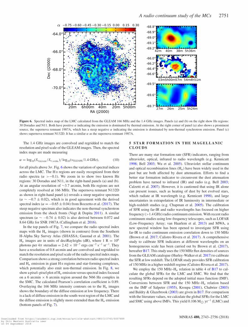
Figure 6. Spectral index map of the LMC calculated from the GLEAM 166 MHz and the 1.4 GHz images. Panels (a) and (b) on the right show HII regions:30 Doradus and N11. Both have positive α indicating the emission is dominated by thermal emission. At the right corner of panel (a) also shows a prominentsource, the supernova remnant 1987A, which has a steep negative α indicating the emission is dominated by non-thermal synchrotron emission. Panel (c)shows supernova remnant N132D. It has a similar α as the supernova remnant 1987A.

The 1.4 GHz images are convolved and regridded to match theresolution and pixel scale of the GLEAM images. Then, the spectralindex maps are made measuring

α = log10(SνGLEAM/Sν1.4 GHz )/ log10(νGLEAM/1.4 GHz), (10)

for all pixels above 3σ . Fig. 6 shows the variation of spectral indicesacross the LMC. The H II regions are easily recognized from theirradio spectra (α >−0.1). We zoom in to show two known HII

regions: 30 Doradus and N11, in the right-hand panels (a) and (b).At an angular resolution of ∼3.7 arcmin, both HII regions are notcompletely resolved at 166 MHz. The supernova remnant N132Das shown in right-hand panel (c) reveals a steep negative spectrum(α ∼ −0.7 ± 0.02), which is in good agreement with the derivedspectral index (α = −0.65 ± 0.04) from Bozzetto et al. (2017). Thesteep negative spectrum also indicates the non-thermal synchrotronemission from the shock fronts (Vogt & Dopita 2011). A similarspectrum (α ∼ −0.74 ± 0.02) is also derived between 0.072 and8.64 GHz for SNR 1987A (Callingham et al. 2016).

In the top panels of Fig. 7, we compare the radio spectral indexmaps with the Hα images (shown in contours) from the SouthernH-Alpha Sky Survey Atlas (SHASSA; Gaustad et al. 2001). TheHα images are in units of deciRayleighs (dR), where 1 R = 106

photons per 4π steradian = 2.42 × 10−7 ergs cm−2 s−1 sr−1. Theyhave a resolution of 0.8 arcmin and are convolved and regridded tomatch the resolution and pixel scale of the radio spectral index maps.Comparison shows a strong correlation between radio spectral indexand Hα emission in giant H II regions and star-forming complexes,which potentially also emit non-thermal emission. In Fig. 8, weshow a pixel–pixel plot of Hα emission versus spectral index focusedon a 6 arcmin × 6 arcmin region around the N66 HII complex inthe SMC. The calculated Pearson’s correlation coefficient is 0.89.Overlaying the 166 MHz intensity contours on to the Hα imagesshows the boundary of the diffuse emission at low frequency. Thereis a lack of diffuse emission in the south-west region of the LMC andthe diffuse emission is slightly more extended than the Hα emission(bottom panels of Fig. 7).

5 STA R FO R M AT I O N IN TH E M AG E L L A N I CC L O U D S

There are many star formation rate (SFR) indicators, ranging fromultraviolet, optical, infrared to radio wavelength (e.g. Kennicutt1998; Bell 2003; Wu et al. 2005). Ultraviolet stellar continuumand optical recombination lines (Hα) have been widely used in thepast but are both affected by dust attenuation. Efforts to find abetter star formation indicator to circumvent the dust attenuationproblem have turned to infrared (IR) and radio (e.g. Bell 2003;Calzetti et al. 2007). However, it is cautioned that using IR alonecan present issues, such as heating of dust by hot evolved stars,which radiate at IR wavelength (e.g. Kennicutt 1998), and largeuncertainties in extrapolation of IR luminosity in intermediate orhigh-redshift studies (e.g. Chapman et al. 2005). The calibrationof SFR using far-IR and radio wavelengths has focused on higherfrequency (>1.4 GHz) radio continuum emission. With recent radiocontinuum studies using low-frequency telescopes, such as LOFAR(Low-Frequency Array; van Haarlem et al. 2013) and MWA, anew spectral window has been opened to investigate SFR usingfar-IR to radio continuum emission correlation down to 150 MHz(Brown et al. 2017; Calistro Rivera et al. 2017). A comprehensivestudy to calibrate SFR indicators at different wavelengths on anhomogeneous scale has been carried out by Brown et al. (2017),hereafter B17. This study uses the 150 MHz flux densities of sourcesfrom the GLEAM catalogue (Hurley-Walker et al. 2017) to calibratethe SFR at low redshift. The LOFAR study provides SFR calibrationof 150 MHz in a higher redshift regime (Calistro Rivera et al. 2017).

We employ the 150 MHz–Hα relation in table 4 of B17 to cal-culate the global SFRs for the LMC and SMC. We find that theresulting SFRs depend on the adopted initial mass function (IMF).Conversions between SFR and the 150 MHz–Hα relation basedon the IMF of Salpeter (1955), Kroupa (2001), Chabrier (2003)and Baldry & Glazebrook (2003) are given in B17. For comparisonwith the literature values, we calculate the global SFRs for the LMCand SMC using above IMFs. This yield 0.106 M� yr−1 (LMC) and

MNRAS 480, 2743–2756 (2018)Downloaded from https://academic.oup.com/mnras/article-abstract/480/2/2743/5057489by Univ Western Australia useron 04 September 2018

2752 B.-Q. For et al.

(b)(a)

(c) (d)

Figure 7. Top panels: Contours of Hα at 2500 dR (black) and 10000 dR (green) overlaid on to the spectral index maps. Bottom panels: Intensity contours of166 MHz continuum map at 0.1 Jy beam−1 (white) and 0.4 Jy beam−1 (green) overlaid on to the SHASSA Hα image.

Figure 8. An example of the relationship between Hα emission and spectralindex in an H II region (N66) in the SMC.

0.033 M� yr−1 (SMC) for the Salpeter IMF, 0.074 M� yr−1 (LMC)and 0.022 M� yr−1 (SMC) for the Kroupa IMF, 0.161 M� yr−1

(LMC) and 0.050 M� yr−1 (SMC) for the Chabrier IMF, 0.068 M�yr−1 (LMC) and 0.021 M� yr−1 (SMC) for the Baldry & Glaze-brook IMF. The global SFR for the LMC is about a factor of 2less than the SFR (∼0.2 M� yr−1) quoted in Hughes et al. (2007),where the Salpeter IMF was used. It is also lower by about a factor of1.5 as compared to 0.037 M� yr−1 in Bolatto et al. (2011), whereKroupa IMF was adopted. The values calculated using ChabrierIMF are more consistent with the literature values that are based onthe 1.4 GHz calibration. The SFR is known to be underestimated atlow frequencies (see e.g. Calistro Rivera et al. 2017).

6 H I I R E G I O N S

The ionizing Lyman continuum photons from young massive OBstars are the cause of their surrounding HII regions. In these regions,the strong correlation between Hα and radio continuum emissionindicates a thermal origin (only α ∼ −0.1). Pellegrini et al. (2012)

MNRAS 480, 2743–2756 (2018)Downloaded from https://academic.oup.com/mnras/article-abstract/480/2/2743/5057489by Univ Western Australia useron 04 September 2018

A radio continuum study of the MCs 2753

Table 5. Lower limit of Lyman continuum photon production rates of selected H II regions in the LMC with α > 0 (see section 6.1).

Source MCELS R.A. (J2000) Decl. (J2000) NUV α

ID (h:m:s) (◦ arcmin arcsec) (s−1)

H II 1 L102 05:05:06.7 −70:06:24.1 7.70 × 1050 –H II 2 L106 05:06:05.0 −65:41:28.7 1.46 × 1051 –H II 3 L119 05:09:34.3 −68:53:44.9 1.40 × 1051 0.05 ± 0.03H II 4 L134 05:12:28.4 −70:24:52.2 2.51 × 1051 –H II 5 L201 05:22:06.9 −67:56:46.0 3.74 × 1051 0.04 ± 0.03H II 6 L258 05:26:42.5 −68:49:34.0 2.52 × 1051 0.12 ± 0.04H II 7 L260 05:27:17.6 −70:34:46.2 8.74 × 1050 –H II 8 L307 05:35:15.6 −67:34:04.1 1.88 × 1051 0.09 ± 0.03H II 9 L328 05:38:36.0 −69:05:10.7 1.06 × 1052 –H II 10 L343 05:40:06.8 −69:45:28.4 2.64 × 1051 0.09 ± 0.03

carried out a study of the optical depth H II regions in the MCsusing the images from the Magellanic Clouds Emission Line Survey(MCELS; Smith & MCELS Team 1998). The study categorized theHII regions into several groups, including optically thin and thick.Using the catalogue of Pellegrini et al. (2012), we first examinedH II regions that are classified as optically thin. If they appear to bepoint sources or not complex at 150 MHz, we extract them as cutoutimages. This results in 46 H II regions for the LMC and 2 H II regionsfor the SMC. Subsequently, we obtain their integrated flux densitiesby fitting a two-dimensional Gaussian to these cutout images. Only10 out of the 46 H II regions in the LMC have converged Gaussianfits, and none for the SMC. The fitting fails to converge if the sourcesappear to have multiple components. The derived Sν are used tocalculate the production rate of Lyman continuum photons (NUV)in the optically thin regime. In this regime, the thermal spectralluminosity (LT) of an H II region is proportional to the productionrate of Lyman continuum photons and varies weakly with electrontemperature (Te) (Rubin 1968). According to Condon (1992), thevalue of NUV (s−1) can be estimated from

NUV

s� 6.3 × 1052

(Te

104K

)−0.45 ( ν

GHz

)0.1(

LT

1020 W Hz−1

).

(11)

We assume Te to be 104 K and note that equation (4) is only ap-plicable to H II regions that are solely thermal. This equation alsoyields a lower limit of NUV due to some Lyman continuum photonsbeing absorbed by dust within the H II regions. The result is shownin Table 5. Among these H II regions, the largest star-forming regionin the LMC, 30 Doradus (source HII 9), has the highest NUV. TheNUV values for the rest of them are of the order of ∼ 1051 s−1, whichis about 10 times higher than the NUV of H II regions in the irregulardwarf galaxy IC 10 (Westcott et al. 2017). A correlation betweenionizing UV flux and radio flux densities for the LMC HII regionshas also been found (see Filipovic, Jones & White 2003).

Studying γ -ray emission in the MCs allows us to probe the phys-ical processes of cosmic rays (CRs) interaction with the interstellarmedium (Ackermann et al. 2016). Discrete sources, in particularlythe star-forming regions, are claimed to be possible sites for pro-ducing large amount of CR-induced γ -ray emission. While we arenot focusing on this topic in this paper, we can estimate the CRconfinement within the LMC and SMC by comparing the contribu-tion from discrete sources to the total Sν . The total integrated fluxdensity of 10 H II regions listed above is ∼138 Jy at 150 MHz, whichincludes the largest H II region (30 Doradus). Based on the LMCdiscrete sources listed in Filipovic et al. (2003), we measure theirSν and yields a total Sν of ∼163 Jy. As for the SMC, we focus on the

H II regions in Pellegrini et al. (2012) and SNRs in Bozzetto et al.(2017). The total Sν from the SMC discrete sources is ∼59 Jy. Theseyield ∼21 per cent and ∼23 per cent of the emission attributed toindividual sources at 150 MHz for the LMC and SMC, respectively.

6.1 T–T plot

To investigate a possible spatial variation of the spectral index acrossthe resolved H II regions in both 227 MHz and 1.4 GHz images, weuse the T–T method (Turtle et al. 1962). This method compares fluxdensity (or brightness temperature) at two frequencies from differ-ent instruments and allows for possible foreground contaminationas well as variations due to short spacings. If there is any differencein short spacings or contamination from foreground emission, itwill result in a non-zero intercept in the T–T plot. We generate theT–T plot by convolving and regridding the LMC 1.4 GHz imageto match the angular resolution and pixel scale of the 227 MHzGLEAM image. The 227 MHz GLEAM image is chosen because ithas the highest angular resolution. Subsequently, we subsample thedata points per 5 pixel (∼1.3 beam separation) in the image plane toremove pixel-to-pixel correlations. Then, we fit the subsampled datausing linear least squares regression. The spectral index is then de-termined by α = log (slope)/c, where c is log (227 MHz/1400 MHz).We present the T–T plots in Fig. 9 and summarize the derived spec-tral indices in Table 5. All fits yield an overall R2 = 0.93, whichsuggests no spatial variation of the spectral index across these H II

regions. We cannot derive spectral indices for five of the H II regionsusing the T–T method because the sources are resolved at 1.4 GHz(multiple components) but not resolved in 227 MHz or affected byartefacts at 1.4 GHz (near the 30 Doradus region). The derived spec-tral indices of these HII regions ranges from ∼0.0 to ∼0.1, whichsuggests a “flat” spectrum dominated by thermal emission. TheseH II regions are in the optically thin regime in the MWA frequencyrange. We also attempted to derive the spectral index and to identifythe turn-over frequency using the optically thick H II regions definedin the catalogue of Pellegrini et al. (2012). However, we do not seeany convincing evidence of a turn over frequency due to difficultyin measuring accurate flux densities in the lower MWA frequencybands as a result of poor resolution.

7 C O N C L U S I O N S

We present a low-frequency radio continuum study of the Mag-ellanic Clouds as part of the GLEAM survey. The intensityof the radio continuum emission is correlated with H I columndensity. Star-forming regions are the main contributors to the

MNRAS 480, 2743–2756 (2018)Downloaded from https://academic.oup.com/mnras/article-abstract/480/2/2743/5057489by Univ Western Australia useron 04 September 2018

2754 B.-Q. For et al.

Figure 9. T–T plots for the five optically thin HII regions in the LMC using 1.4 GHz and 227 MHz images. The 1.4 GHz cutout images have been convolvedand regridded to match the resolution and pixel scale of the 227 MHz images. The data points have been subsampled every 5 pixel in the image plane. Thefitted lines are the spectral indices of these regions. Error of S1400 is ∼0.3 mJy beam−1, which makes the error bars too small to be visible in these plots.

emission. Intensity variation is noticeable in the LMC but flat acrossthe bar of the SMC. We derive spectral indices of the MCs using200 MHz as a reference frequency. A double power-law model isrequired to fit the SED of the LMC. The fitted model yields α0 =−0.66 ± 0.08 (non-thermal) when α1 (thermal) is fixed at −0.1. Apower-law model is preferred for the SMC, which yields α85.5MHz

8.55GHz(SMC) =−0.82 ± 0.03. Spectral index maps show a variation of α

across the Magellanic Clouds, which reflects the presence of ther-

mal and non-thermal components. H II regions have a distinctiveflat spectral index and strongly correlate with Hα , indicating mainlythermal emission. We also calculate the lower limit production rateof Lyman continuum photons of ten HII regions in the LMC usingtheir integrated flux density at 150 MHz. An investigation of spec-tral index variation among the H II regions is carried out using theT–T method. The derived spectral indices for these HII regions arebetween about 0 and 0.1. The new Hα–150 MHz SFR calibrations

MNRAS 480, 2743–2756 (2018)Downloaded from https://academic.oup.com/mnras/article-abstract/480/2/2743/5057489by Univ Western Australia useron 04 September 2018

A radio continuum study of the MCs 2755

(Brown et al. 2017) allow us to determine the global SFRs of theMCs. Using their calibrations based on Salpeter, Kroupa, Chabrierand Baldry & Glazebrook’s IMFs, we obtain the global SFRs of0.068–0.161 M� yr−1 and 0.021–0.050 M� yr−1 for the LMC andSMC, respectively. We find that the global SFRs are consistent withthe 1.4 GHz SFR calibration if Charbrier’s IMF is adopted. Robust-1 images in 20 frequency bands and wideband averages are madeavailable at the GLEAM Virtual Observatory (VO) server.2

8 FU T U R E WO R K

A detailed study of discrete sources such as H II regions, super-nova remnants, and background sources in the GLEAM imageswill be presented in a subsequent paper. An analysis of the radio-FIR correlation has been performed in the past for the MCs (Hugheset al. 2006; Leverenz & Filipovic 2013). These studies focused on1.4 GHz and Infrared Astronomical Satellite (IRAS) images. Fu-ture work includes an investigation of the radio-FIR correlation ondifferent spatial scales using MWA and Herschel images (as part ofthe HERschel Inventory of The Agents of Galaxy Evolution survey;HERITAGE; Meixner et al. 2013). A deep survey of the MagellanicSystem (MAGE-X; led by L. Staveley-Smith) using the MWA phaseII system has been commenced. The survey will focus on quantify-ing the energy spectrum of cosmic ray electrons at higher angularresolution.

AC K N OW L E D G E M E N T S

This scientific work makes use of the Murchison Radio-astronomyObservatory, operated by CSIRO. We acknowledge the Wajarri Ya-matji people as the traditional owners of the Observatory site. Sup-port for the operation of the Murchison Widefield Array is providedby the Australian Government (NCRIS), under a contract to CurtinUniversity administered by Astronomy Australia Limited. We ac-knowledge the Pawsey Supercomputing Centre which is supportedby the Western Australian and Australian Governments and theCentre of Excellence for All-sky Astrophysics (CAASTRO), whichis an Australian Research Council Centre of Excellence, funded bygrant CE110001020. Parts of this research were conducted with thesupport of Australian Research Council Centre of Excellence for AllSky Astrophysics in 3 Dimensions (ASTRO 3D), through projectnumber CE170100013. This research also made use of Montage.Montage is funded by the National Science Foundation under GrantNumber ACI-1440620, and was previously funded by the NationalAeronautics and Space Administration’s Earth Science Technol-ogy Office, Computation Technologies Project, under CooperativeAgreement Number NCC5-626 between NASA and the CaliforniaInstitute of Technology.

RE FER ENCES

Ackermann M. et al., 2016, A&A, 586, A71Alvarez H., Aparici J., May J., 1987, A&A, 176, 25Baars J. W. M., Genzel R., Pauliny-Toth I. I. K., Witzel A., 1977, A&A, 61,

99Baldry I. K., Glazebrook K., 2003, ApJ, 593, 258Bell E. F., 2003, ApJ, 586, 794Besla G., Martınez-Delgado D., van der Marel R. P., Beletsky Y., Seibert

M., Schlafly E. F., Grebel E. K., Neyer F., 2016, ApJ, 825, 20

2http://gleam-vo.icrar.org/gleam postage/q/form

Blackburn J. K., 1995, in Shaw R. A., Payne H. E., Hayes J. J. E., eds, ASPConf. Ser. Vol. 77, Astronomical Data Analysis Software and SystemsIV. Astron. Soc. Pac., San Francisco, p. 367

Bolatto A. D., Leroy A., Israel F. P., Jackson J. M., 2003, ApJ, 595, 167Bolatto A. D. et al., 2011, ApJ, 741, 12Bowman J. D. et al., 2013, PASA, 30, e031Bozzetto L. M. et al., 2017, ApJS, 230, 2Briggs D. S., 1995, Bull. Am. Astron. Soc., 27, 1444Brown M. J. I. et al., 2017, ApJ, 847, 136 (B17)Bruns C. et al., 2005, A&A, 432, 45Calistro Rivera G. et al., 2017, MNRAS, 469, 3468Callingham J. R. et al., 2016, MNRAS, 462, 290Calzetti D. et al., 2007, ApJ, 666, 870Chabrier G., 2003, PASP, 115, 763Chapman S. C., Blain A. W., Smail I., Ivison R. J., 2005, ApJ, 622, 772Chen C.-H. R. et al., 2014, ApJ, 785, 162Condon J. J., 1992, ARA&A, 30, 575Diaz J., Bekki K., 2011, PASA, 28, 117Feitzinger J. V., Perschke M., Haynes R. F., Klein U., Wielebinski R., 1987,

Vistas in Astron., 30, 243Filipovic M. D., Haynes R. F., White G. L., Jones P. A., 1998, A&AS, 130,

421Filipovic M. D., Bohlsen T., Reid W., Staveley-Smith L., Jones P. A., Nohejl

K., Goldstein G., 2002, MNRAS, 335, 1085Filipovic M. D., Jones P. A., White G. L., 2003, Serb. Astron. J., 166Gaustad J. E., McCullough P. R., Rosing W., Van Buren D., 2001, PASP,

113, 1326Harris J., 2007, ApJ, 658, 345Harvey V. M., Franzen T., Morgan J., Seymour N., 2018, MNRAS, 476,

2717Haslam C. G. T., Klein U., Salter C. J., Stoffel H., Wilson W. E., Cleary M.

N., Cooke D. J., Thomasson P., 1981, A&A, 100, 209Haynes R. F. et al., 1991, A&A, 252, 475Helou G., Bicay M. D., 1993, ApJ, 415, 93Hilditch R. W., Howarth I. D., Harries T. J., 2005, MNRAS, 357, 304Hughes A., Wong T., Ekers R., Staveley-Smith L., Filipovic M., Maddison

S., Fukui Y., Mizuno N., 2006, MNRAS, 370, 363Hughes A., Staveley-Smith L., Kim S., Wolleben M., Filipovic M., 2007,

MNRAS, 382, 543Hurley-Walker N. et al., 2017, MNRAS, 464, 1146Jameson K. E. et al., 2016, ApJ, 825, 12Kallivayalil N., van der Marel R. P., Besla G., Anderson J., Alcock C., 2013,

ApJ, 764, 161Kass R. E., Raftery A. E., 1995, J. Am. Stat. Assoc., 90, 773Kennicutt R. C., Jr, 1998, ARA&A, 36, 189Kim S., Staveley-Smith L., Dopita M. A., Sault R. J., Freeman K. C., Lee

Y., Chu Y.-H., 2003, ApJS, 148, 473Klein U., Wielebinski R., Haynes R. F., Malin D. F., 1989, A&A, 211, 280Kroupa P., 2001, MNRAS, 322, 231Leverenz H., Filipovic M. D., 2013, Ap&SS, 343, 301Lisenfeld U., Volk H. J., 2000, A&A, 354, 423Loiseau N., Klein U., Greybe A., Wielebinski R., Haynes R. F., 1987, A&A,

178, 62Lonsdale C. J. et al., 2009, IEEE Proceedings, 97, 1497Mackey A. D., Koposov S. E., Erkal D., Belokurov V., Da Costa G. S.,

Gomez F. A., 2016, MNRAS, 459, 239Marvil J., Owen F., Eilek J., 2015, AJ, 149, 32Meixner M. et al., 2013, AJ, 146, 62Mills B. Y., 1955, Aust. J. Phys., 8, 368Mills B. Y., 1959, Handbuch der Physik, 53, 239Mountfort P. I., Jonas J. L., de Jager G., Baart E. E., 1987, MNRAS, 226,

917Ochsendorf B. B., Zinnecker H., Nayak O., Bally J., Meixner M., Jones O.

C., Indebetouw R., Rahman M., 2017, Nature Astron., 1, 268Offringa A. R. et al., 2015, PASA, 32, e008Pellegrini E. W., Oey M. S., Winkler P. F., Points S. D., Smith R. C., Jaskot

A. E., Zastrow J., 2012, ApJ, 755, 40Pietrzynski G. et al., 2013, Nature, 495, 76

MNRAS 480, 2743–2756 (2018)Downloaded from https://academic.oup.com/mnras/article-abstract/480/2/2743/5057489by Univ Western Australia useron 04 September 2018

2756 B.-Q. For et al.

Rubin R. H., 1968, ApJ, 154, 391Salpeter E. E., 1955, ApJ, 121, 161Schwarz G., 1978, Ann. Statist., 5, 461Shain C. A., 1959, in Bracewell R. N., ed., IAU Symp. 9, Observations of

Extragalactic Radio Emission. Stanford Univ. Press, Stanford, CA, p.328

Smith R. C., MCELS Team, 1998, PASA, 15, 163Stanimirovic S., Staveley-Smith L., Dickey J. M., Sault R. J., Snowden S.

L., 1999, MNRAS, 302, 417Staveley-Smith L., Sault R. J., Hatzidimitriou D., Kesteven M. J., McConnell

D., 1997, MNRAS, 289, 225Staveley-Smith L., Kim S., Calabretta M. R., Haynes R. F., Kesteven M. J.,

2003, MNRAS, 339, 87Tingay S. J. et al., 2013, PASA, 30, e007Turtle A. J., Pugh J. F., Kenderdine S., Pauliny-Toth I. I. K., 1962, MNRAS,

124, 297van der Marel R. P., Kallivayalil N., 2014, ApJ, 781, 121van Haarlem M. P. et al., 2013, A&A, 556, A2Vogt F., Dopita M. A., 2011, Ap&SS, 331, 521Wayth R. B. et al., 2015, PASA, 32, e025Westcott J. et al., 2017, MNRAS, 467, 2113Wu H., Cao C., Hao C.-N., Liu F.-S., Wang J.-L., Xia X.-Y., Deng Z.-G.,

Young C. K.-S., 2005, ApJ, 632, L79Zanardo G. et al., 2010, ApJ, 710, 1515

1International Centre for Radio Astronomy Research, University of WesternAustralia, 35 Stirling Hwy, Crawley, WA 6009, Australia2ARC Centre of Excellence for All Sky Astrophysics in 3 Dimensions (ASTRO3D)3ARC Centre of Excellence for All-sky Astrophysics (CAASTRO)4International Centre for Radio Astronomy Research, Curtin University,Bentley, WA 6102, Australia5National Radio Astronomy Observatory (NRAO), Socorro, NM 87801, USA6School of Computing Engineering and Mathematics, Western Sydney Uni-versity, Locked Bag 1797, Penrith, NSW 2751, Australia7CSIRO Astronomy and Space Science (CASS), PO Box 76, Epping, NSW1710, Australia8The Inter-University Institute for Data Intensive Astronomy (IDIA), De-partment of Astronomy, University of Cape Town, Rondebosch, 7701, SouthAfrica

9Netherlands Institute for Radio Astronomy (ASTRON), Dwingeloo, theNetherlands10University of Technology Sydney, 15 Broadway, Ultimo NSW 2007, Aus-tralia11Department of Physics and Electronics, Rhodes University, PO Box 94,Grahamstown 6140, South Africa12School of Earth and Space Exploration, Arizona State University, Tempe,AZ 85287, USA13Research School of Astronomy and Astrophysics, Australian National Uni-versity, Canberra, ACT 2611, Australia14MIT Haystack Observatory, Westford, MA 01886, USA15Raman Research Institute, Bangalore 560080, India16Dunlap Institute for Astronomy and Astrophysics, University of Toronto,ON, M5S 3H4, Canada17Sydney Institute for Astronomy, School of Physics, The University of Syd-ney, NSW 2006, Australia18Harvard-Smithsonian Center for Astrophysics, Cambridge, MA 02138,USA19Department of Physics, University of Washington, Seattle, WA 98195,USA20Centre for Astrophysics Research, School of Physics, Astronomy andMathematics, University of Hertfordshire, College Lane, Hatfield AL10 9AB,UK21Peripety Scientific Ltd., PO Box 11355 Manners Street, Wellington 6142,New Zealand22Department of Physics, University of Wisconsin–Milwaukee, Milwaukee,WI 53201, USA23School of Physics, The University of Melbourne, Parkville, VIC 3010,Australia24Kavli Institute for Astrophysics and Space Research, Massachusetts Insti-tute of Technology, Cambridge, MA 02139, USA25National Centre for Radio Astrophysics, Tata Institute for FundamentalResearch, Pune 411007, India26School of Engineering & Computer Science, Victoria University ofWellington, PO Box 600, Wellington 6141, New Zealand

This paper has been typeset from a TEX/LATEX file prepared by the author.

MNRAS 480, 2743–2756 (2018)Downloaded from https://academic.oup.com/mnras/article-abstract/480/2/2743/5057489by Univ Western Australia useron 04 September 2018