a multiwavelength study of tev blazarshagar/phd/thesis_as.pdfa multiwavelength study of tev blazars...
TRANSCRIPT
A Multiwavelength study of TeV blazars
A Thesis
Submitted to the
Tata Institute of Fundamental Research, Mumbai
for the degree of Doctor of Philosophy
in Physics
by
Atreyee Sinha
School of Natural Sciences
Tata Institute of Fundamental Research
Mumbai
September, 2016
Final Version Submitted in December, 2016


To my dearest cousin, Pounomi
(1993 - 2015)
- One of the most creative and interesting persons
I have ever met.


Declaration
DECLARATION
This thesis is a presentation of my original research work. Wherever contributions of
others are involved, every effort is made to indicate this clearly, with due reference to
the literature, and acknowledgement of collaborative research and discussions.
The work was done under the guidance of Dr. Varsha R Chitnis, at the Tata Institute of
Fundamental Research, Mumbai.
Atreyee Sinha
In my capacity as supervisor of the candidate’s thesis, I certify that the above statements
are true to the best of my knowledge.
Dr.. Varsha R Chitnis
Date:

“No man is an island entire of itself; every man is a piece
of the continent, a part of the main.
John DonneAcknowledgements
Doing justice to the acknowledgements must be one of the hardest parts of writing a
thesis. How do I express my gratitude towards all the people without whose contribution
this would never have been possible?
Firstly, to my advisor, Dr. Varsha Chitnis. It is, but a rare chance, to find an advisor
who lets you explore, gives you wings to fly, and yet, keeps you firmly grounded, always
available for guidance. I am indeed lucky to have been your student.
I have greatly benefited from discussions with many of the esteemed faculty at our
institute; Prof. Acharya, who has been a very close mentor... I truly learnt a lot about the
basics of high energy cosmic rays during our interactions; Prof. Rao for his keen insights
into X-ray instrumentation; Prof. Yadav, for letting me work on LAXPC data, something
which I have really enjoyed; Prof. Krishnan and Prof. Dasgupta, for their helpful
comments during my synopsis; Prof. Gopakumar for many stimulating conversations;
Prof. Arnab Bhattacharya and Kulkarniji for letting me be a part of the vibrant outreach
team... during the depressing months of compilation errors and journal rejections, the
outreach activities served to remind me why I came to love physics in the first place.
It would not be an exaggeration to say that I would have learnt nothing of blazar
physics had it not been for the constant guidance and encouragement of Dr. Sahayanathan
from BARC. You have been the driving force behind this work. Our collaboration with
Prof. Misra at IUCAA counts among the most enjoyable moments of my PhD.
I am extremely lucky to have been blessed with a family that loves me unconditionally,
through all my ups and downs; my parents, who first introduced me to the excitement of
science, who let me choose my career and my future without any hesitation, who have
always been there for me; my sister Ayesha, the first friend I have had, my fiercest critic
and the first person to stand up for me, I hope someday I will be worthy of the standards
you hold me up to; my late grandmother, who made me what I am; my Mamaji Arup
and his family, whose place has been the one stop solution whenever I have been in need
of money, food, sleep or comfort; my maternal grandparents, who have always believed
in me (even at times I did not).
I could not have gone through the stress of graduate school without the wonderful
environment at TIFR. Thanks to my seniors, especially Sayan, Samashis, Sanmay, Gourab,
Kolahal and his wife Tamali, Lab and his wife Amrita, Nilay, Sumanta, Umesh, Sunil
and Pankaj, for creating such wonderful memories and still being just an email away
whenever I need any advice, academic or otherwise. It is hard to thank my friends enough
for their contribution; Khadiza, friends like you give meaning to human bondings, I am
blessed to have had you as my roommate; Chitrak and Nairit, you made me take the
hardest look at myself, and changed me so much for the better; Shubhadeep, I think I

vi
would have given up a long time ago without your support; Ritam, for understanding
me better than anyone else. Thanks to Debjyoti, Soureek, Joe, Gope, Nilakash, Rickmoy
and Tanusree for all the times we spent together.
Special mention must be made of my time at Hanle; it was an enthralling experience
which will stay with me till my last breath. Thanks to all the engineers and support staff
at the HAGAR facility for having made the stay so special... I will never forget the 3 am
Maggi we used to have there.
I have been lucky to have attended many conferences and schools all over the country,
and have learnt a lot from the discussions we had. Thanks to, among other, Pratikda,
Gulab, Somadi, Nijil, Sagar, Nilay, Subirda, Stalin, Preeti and Prajwal.
Thanks to all my teachers and friends from school and college, for encouraging my
dreams and sharing in my joy... specially my computer teacher, Suparna Miss and physics
teachers, Susmita Miss and Binoy Sir, and my friends Sucharita, Asmi, Maddy and Tirtho.
And last, because perhaps it’s the most difficult to express, to my fiancee Debayan;
you have, without complaints, borne the brunt of my mood swings over the past decade.
Thanks for loving me at my worst, and yet, bringing out the best in me; always.
A. Sinha A Multiwavelength Study of TeV Blazars

0Synopsis
0.1 I N T R O D U C T I O N
An active galactic nucleus (AGN) is a compact region (∼ light days) at the centre of a
galaxy that outshines the total emission from the remaining of the host galaxy. Such
excess emission has been observed across the entire electromagnetic spectrum, from
radio to γ-rays, and is believed to be powered by accretion onto super-massive black
holes (Salpeter, 1964; Lynden-Bell, 1969). Depending upon the ratio of the radio (5
GHz) to optical (B band) flux, AGNs are further classified as radio-loud and radio quiet.
Around 10-15% of the AGNs are radio-loud (Urry & Padovani, 1995), and observationally
exhibit prominent bipolar radio jets reaching up to Mpc scales.
Blazars count among the most violent sources of high energy emission in the known
universe. They are characterized by highly variable nonthermal emission across the
entire electromagnetic spectrum, strong radio and optical polarization, and apparent
superluminal motion. According to the classification scheme of Urry & Padovani (1995),
the likely explanation of such observations is that they are a subclass of radio-loud AGNs
where the relativistic jet is oriented close to the line of sight. Based on the rest frame
equivalent width of their emission lines in optical/UV spectra, blazars have been further
classified in two subgroups: BL Lacertae objects (BL Lacs) with very weak/no emission
lines and Flat Spectrum Radio Quasars (FSRQ) with strong broad-line emission.
The broadband spectral energy distribution (SED) of blazars is characterized by two
peaks, one in the IR - X-ray regime, and the second one in the γ-ray regime. According
to the location of the first peak, BL Lacs are further classified into low-energy peaked
BL Lacs (LBL), intermediate peaked BL Lacs (IBL) and high-energy peaked BL Lacs (HBL)
(Padovani & Giommi, 1995). Both leptonic and hadronic models have been used to
explain the broadband SED with varying degrees of success. The origin of the low-energy
component is well established to be caused by synchrotron emission from relativistic
electrons gyrating in the magnetic field of the jet. However, the physical mechanisms
responsible for the high-energy emission are still under debate. It can be produced
either through inverse Compton (IC) scattering of low-frequency photons by the same
electrons responsible for the synchrotron emission (leptonic models), or through hadronic
processes initiated by relativistic protons, neutral and charged pion decays, or muon
cascades (hadronic models). The seed photons for IC in leptonic models can be either
the synchrotron photons themselves (synchrotron self-Compton, SSC) or from external
vii
viii
S Y N O P S I S
0.1 I N T R O D U C T I O N
sources such as the broad line region (BLR), the accretion disc, and the cosmic microwave
background (external Compton, EC). A comprehensive review of these mechanisms may
be found in Böttcher (2007).
The advent of the Atmospheric Cherenkov Telescopes (ACT) opened a new window
into blazar research. The first significant detection of extragalactic TeV photons was
from the blazar Mkn 421 by the Whipple collaboration in 1992 (Punch et al., 1992).
Since then, over 55 blazars (Wakely & Horan, 2016) have been detected in the very high
energy (VHE) regime, and form the dominant source of high energy radiation in the
extragalactic sky.
When a VHE gamma-ray enters into the Earth’s atmosphere, it interacts with atmo-
spheric nuclei and produces an electron-positron pair, which in turn dissipates its energy
producing secondary gamma rays through bremsstrahlung processes. The secondary
gamma rays further produce electron-positron pairs. This process of pair production and
bremsstrahlung continues, resulting in a shower of electrons, positrons and secondary
gamma rays, which is called an Extensive Air Shower (EAS). When the charged particles
move down in the atmosphere with velocities greater than the velocity of the light in that
medium, they produce Cherenkov light, which falls in Ultra Violet and blue (UV-blue)
region of the electromagnetic spectrum. The Cherenkov light illuminates a large circular
area with a diameter in the range of 200 m - 250 m on the ground for a vertically incident
shower. This light can be captured with optical sensors, and by reconstructing the shower
axis in space and tracing it back onto the sky, celestial origin of the gamma rays can be
determined. The energy of the primary γ-ray can be estimated from the intensity of the
Cherenkov light pool.
The High Altitude GAmma Ray (HAGAR) (Chitnis et al., 2011) array is a hexagonal
array of seven ACTs which uses the wavefront sampling technique to detect celestial
gamma rays. It is located at the Indian Astronomical Observatory site (32 46’ 46" N,
78 58’ 35" E), in Hanle, Ladakh in the Himalayan mountain ranges at an altitude of
4270m. The Cherenkov photon density of a shower increases with altitude, and thus,
a lower energy threshold is achieved by operating the telescope at such high altitudes.
Each of the seven telescopes has seven para-axially mounted front coated parabolic glass
mirrors of diameter 0.9 m, with a UV-sensitive photo-multiplier tube (PMT) at the focus
of individual mirrors. The Cherenkov photons arriving at each telescope are detected by
these PMTs. The relative arrival time of the Cherenkov shower front at each telescope is
recorded for each event using a 12 bit Phillips Time to Digital Converter (TDC), which is
then used to reconstruct the initial shower direction by the triangulation method. The
energy threshold for the HAGAR array for vertically incident γ-ray showers is 208 GeV,
with a sensitivity of detecting a Crab nebula like source in 17hr for a 5σ significance.
Detailed descriptions of HAGAR instrumentation and simulations can be found in Shukla
et al. (2012) and Saha et al. (2013).
Studies at TeV energies are complicated due to the fact that VHE photons emitted
from blazars are absorbed en-route by forming electron-positron pairs on interaction
A. Sinha A Multiwavelength Study of TeV Blazars
S Y N O P S I S
0.2 M O T I VAT I O N A N D A I M S ix
with the photons of the extra-galactic background light (EBL), thereby causing the
observed spectrum to differ significantly from the intrinsic one. The EBL is an isotropic
diffuse radiation field extending from Ultraviolet (UV) to Infrared (IR) wavelength
(λ= 0.1 − 1000µm). It is the relic radiation containing information about the structure
formation epoch of the universe and hence, is an important cosmological quantity (Dwek
& Krennrich, 2013; De Angelis et al., 2013). Direct measurement of EBL is very difficult
due to strong foreground contamination by the Galactic and zodiacal light, and depends
on the choice of the zodiacal light models (Kelsall et al., 1998; Wright, 1998). However,
different upper and lower limits on EBL, based on various observations and deep galaxy
number counts, have been put forth (Hauser et al., 1998; Madau & Pozzetti, 2000;
Domínguez et al., 2011; Helgason & Kashlinsky, 2012). Theoretical prediction of the
EBL SED can be obtained by evolving stellar populations and galaxies under various
cosmological initial conditions (Primack et al., 2005; Franceschini et al., 2008; Gilmore
et al., 2009; Finke et al., 2010; Kneiske & Dole, 2010). However, such models involve a
large number of parameters and the estimated EBL spectrum depends upon the underlying
assumptions (Hauser & Dwek, 2001; de Angelis et al., 2009; Dwek & Krennrich, 2013).
0.2 M O T I VAT I O N A N D A I M S
Blazars are the ideal objects for studying the physics of the ubiquitous but poorly under-
stood astrophysical jets. The jet formation, collimation and acceleration are still only
vaguely understood. The observed rapid variability suggests that the emission region is
compact and located close to the nucleus (Dondi & Ghisellini, 1995), which lies below
the resolution limit of modern facilities. Thus, even the sites of production of radiation
at different energies are also not well known.
In such a scenario, multi-wavelength temporal and spectral studies offer powerful
diagnostics to study the underlying blazar environment. Moreover, indirect estimation of
the EBL intensity can be obtained by studying its imprint on the VHE spectrum of blazars.
Various constraints have been imposed on the EBL intensity under different assumptions
of the intrinsic blazar spectrum (Madau & Phinney, 1996; Coppi & Aharonian, 1999;
Stanev & Franceschini, 1998; Aharonian et al., 2006b; Mazin & Raue, 2007; Guy et al.,
2000; Orr et al., 2011). However, these estimates depend heavily on the assumption of
the intrinsic VHE spectrum, which itself is not well known.
In this work, we have tried to obtain a model independent estimate of the EBL from a
statistical study of TeV blazars. We have also tried to understand the intrinsic particle
spectrum in the jets through a thorough temporal and spatial study of HAGAR observed
blazars in the ambit of leptonic models.
A Multiwavelength Study of TeV Blazars A. Sinha
x
S Y N O P S I S
0.3 M E T H O D O L O GY
0.3 M E T H O D O L O GY
The HAGAR Telescope has been regularly observing bright blazars since its inception in
2008. Data obtained over the past few years were analysed and integral flux (or 3-σ
flux upper limits) computed. Monthly averaged calibration runs were used to calculate
the fixed time offsets of the telescopes, which were then used for reconstruction of
arrival direction of the shower front. The source counts were computed according to the
procedure outlined in Shukla et al. (2012), with appropriate data selection cuts imposed.
Only events with signals in at least 5 telescopes were retained to minimize the systematic
errors, for which the energy threshold was estimated to be ∼ 250GeV .
In addition, data from the Fermi-LAT, NuSTAR, Swift X-ray and UV telescopes were
analyzed according to the standard procedures suggested by the respective instrument
teams. X-ray observations by the Monitor of All-sky X-ray Image (MAXI) telescope, optical
observations by SPOL CCD Imaging/Spectropolarimeter at Steward Observatory, Arizona
and radio data from the Owens Valley Radio Observatory (OVRO), California were also
used to construct the SEDs and light-curves.
We quantified the variability at different wavelengths using the fractional variability
amplitude parameter Fvar , defined in (Vaughan et al., 2003; Chitnis et al., 2009). To
study the time lags between the various unevenly sampled energy bands, we used the
z-transformed discrete cross correlation function, freely available as a FORTRAN 90
routine, with the details of the method described in Alexander (1997).
Signatures of lognormality were investigated for by fitting the histograms of the
observed fluxes at different wavelengths with a Gaussian and a Lognormal function.
To test the rms-flux relationship, following Giebels & Degrange (2009); Chevalier et al.
(2015), the scatter plot of the excess variance vs the mean flux was fit by a constant and
a linear function.
The SEDs were modelled with a one zone leptonic model, incorporating synchrotron
and SSC processes. In this model, the broadband emission is assumed to originate
from a single spherical zone of radius R filled with a tangled magnetic field B. A non-
thermal population of electrons is assumed to lose its energy through synchrotron and self
Compton (SSC) processes. As a result of the relativistic motion of the jet, the radiation is
boosted along our line of sight by a Doppler factor δ. The numerical codes developed in
Sahayanathan & Godambe (2012) and Saha & Bhattacharjee (2015) were incorporated
in the XSPEC spectral fitting software to perform a χ2 minimization (Sahayanathan et al.,
2016).
The EBL density was estimated by looking at its imprint on the VHE spectrum of HBLs.
We computed the Spearman’s rank correlation between the spectral index at different
wavelengths vs the redshift. It was found that very high energy (VHE) gamma ray spectral
index of high energy peaked blazars correlates strongly with its corresponding redshift
whereas no such correlation is observed in the X-ray or the GeV bands. Attributing this
A. Sinha A Multiwavelength Study of TeV Blazars
S Y N O P S I S
0.4 R E S U LT S xi
correlation to a result of photon-photon absorption of TeV photons with the extragalactic
background light (EBL), the allowed flux range for the EBL was constrained.
0.4 R E S U LT S
We concentrated on studying the most abundant blazar subclass in the TeV sky, the HBLs.
The HBLs constitute more than 80% of TeV detected blazars, and usually do not require
an EC mechanism to explain the observed γ-ray spectrum.
0.4.1 Longterm study of Mkn 421
In Sinha et al. (2016b), we studied the long term temporal and spectral variability in
the radiation from the nearby HBL Mkn 421 during 2009-2015. One of the closest
(z = 0.031) and the best-studied TeV blazars, Mkn 421 is also one of the brightest
BL Lac objects seen in the UV and X-ray bands. In this paper we presented the results
of the long term monitoring of this source by the HAGAR telescope array for the past
7 years, since 2009. We used data at the radio, optical, X-ray and gamma ray energies
to characterize lognormality in the intrinsic flux variations across the multi-wavelength
spectrum. Correlation studies between different wavelengths were also performed.
Spectral energy distribution during different flux states of the source were constructed
simultaneous with HAGAR observations, and fit with leptonic SSC models. The main
aim of this paper was not to investigate the fast temporal and spectral variabilities, but
to study the smooth variations over weekly and monthly timescales, which may throw
light on the underlying jet environment.
The multi-wavelength lightcurve of Mkn 421 from all available instruments during
2009-2015 was studied in details. The flux was found to be highly variable across all
time scales. The variability was energy dependent, and maximum in the X-ray and VHE
bands. A strong correlation was found between the Fermi-LAT (gamma) and radio bands,
and between Fermi-LAT and optical, but none between Fermi-LAT and X-ray.
Lognormality in the flux distribution, and a strong flux-rms correlation was seen.
Lognormality was clearly detected for the survey instruments, Fermi-LAT, Swift-BAT and
MAXI, but the correlations decreased for the other instruments. This is likely due to
the fact that the observations from the pointing instruments were biased towards the
flaring states. This is the third blazar, following BL Lac and PKS 2155+304 to show this
behaviour.
Twenty one SEDs were extracted over the past 7 years, during epochs contemporaneous
with HAGAR observation periods. During these epochs, the total bolometric luminosity
varied almost by a factor of 10. All the states could be successfully fitted by our SSC
model, and variations in the flux states attributed mainly to changes in the particle
distribution. A strong correlation was seen between the break energy γb of the particle
A Multiwavelength Study of TeV Blazars A. Sinha

xii
S Y N O P S I S
0.4 R E S U LT S
spectrum and the total bolometric luminosity. During all the epochs, the energy density
in the jet was matter dominated, with the model parameters a factor of 10 away from
equipartition.
0.4.2 Study of Mkn 421 during giant X-ray flare
The largest X-ray flare of Mkn 421 over the past decade was seen during April 2013
(MJD 56392−56403). In Sinha et al. (2015), we undertook a multi-wavelength study
of this flare, with emphasis on the X-ray data to understand the underlying particle
energy distribution. The flux varied rapidly in the X-ray band, with a minimum doubling
timescale of 1.69±0.13 hr. There were no corresponding flares in UV and gamma-ray
bands. The variability in UV and gamma rays was relatively modest with ∼ 8% and
∼ 16%, respectively, and no significant correlation was found with the X-ray light curve.
We modeled the underlying particle energy spectrum with a single population of
electrons emitting synchrotron radiation, and statistically fitted the simultaneous time-
resolved data from Swift-XRT and NuSTAR. The observed X-ray spectrum showed a clear
curvature that could be fit by a log parabolic spectral form. This was best explained as
originating from a log parabolic electron spectrum. However, a broken power law or
a power law with an exponentially falling electron distribution could not be ruled out
either.
Moreover, the excellent broadband spectrum from 0.3−79 keV allowed us to make
predictions of the UV flux. We found that this prediction was compatible with the observed
flux during the low state in X-rays. However, during the X-ray flares, depending on the
adopted model, the predicted flux was a factor of 2−50 lower than the observed one. A
plausible interpretation of this inconsistency between X-ray and UV fluxes could be made
by associating the UV emission from the putative accretion disk. However, such thermal
emission from the disc has never been an important contribution in the UV bands for
Mkn 421 Abdo et al. (2011a), and the UV spectral detail was not sufficient to support this
interpretation. Alternatively, the underlying particle distribution might be more complex
than those we studied. Nevertheless, such a particle distribution demands a concave
spectrum, which is not possible with our present understanding of particle acceleration
(Sahayanathan, 2008). Hence, we attributed this unusual X-ray - UV behaviour of the
source to a two-population electron distribution.
0.4.3 Multi-epoch multi-wavelength study of 1ES 1011+496
1ES 1011+496 is a HBL located at a redshift of z = 0.212. It was discovered as a VHE
emitter by the MAGIC collaboration in 2007, following an optical outburst in March
2007 (Albert et al., 2007b). At its epoch of discovery, it was the most distant TeV source.
Albert et al. (Albert et al., 2007b) had constructed the SED with simultaneous optical
A. Sinha A Multiwavelength Study of TeV Blazars

S Y N O P S I S
0.4 R E S U LT S xiii
R-band data, and other historical data (Costamante & Ghisellini, 2002) and modelled it
with a single zone radiating via SSC processes. However, the model parameters could
not be constrained due to the sparse sampling and the non-simultaneity of the data.
In February 2014, 1ES 1011+496 was reported to be in its highest flux state till date as
seen by Fermi-LAT (Corbet & Shrader, 2014), and Swift-XRT (Kapanadze, 2014). During
this time, the VERITAS collaboration also detected a strong VHE flare from this source,
at an integral flux level of ∼ 20% to 75% of the Crab flux, which is almost a factor of
10 higher than its baseline flux (Cerruti, 2015b). This source was observed by the High
Altitude GAmma Ray (HAGAR) Telescope array during the February-March 2014 season.
In Sinha et al. (2016a), we studied the simultaneous SED of this source as seen by
Swift, Fermi-LAT and HAGAR during this epoch. To understand the broadband spectral
behaviour, we also constructed SEDs using quasi-simultaneous data of two previous
epochs.
It was observed that the broadband SED could be successfully reproduced by syn-
chrotron and synchrotron self Compton emission models. However, the observed curva-
ture in the photon spectrum at X-ray energies could not be explained by an underlying
broken power law (BPL) electron spectrum, but demanded a gradual curvature in the
particle spectrum, eg: a smooth broken power law or a cutoff power law. The different
flux states could be reproduced by mainly changing the particle indices and the break
energy; whereas, the variations in other parameters like the Doppler factor and the
magnetic field were minimal. While the total bolometric luminosity, L, changed by more
than a factor of 3, the variations in B and δ were less than 10%.
To investigate the origin of a curved particle distribution, the time dependent kinetic
equation (Kardashev, 1962) was solved under appropriate assumptions using the Green’s
function technique (Atoyan & Aharonian, 1999). It was found that an energy dependent
escape rate of particles from the emission region gives rise to a smooth curvature in
the particle spectrum. Specifically, particles escaping at a rate proportional to E0.7 give
rise to a particle spectrum consistent with the one described by the power law with an
exponentially decreasing tail.
0.4.4 EBL estimation from VHE observations
Before the year 2000, the number of blazars detected at VHE energies were few(∼ 4),
primarily due to low sensitivity of first generation atmospheric Cherenkov telescopes
(Costamante & Ghisellini, 2002). However, with the advent of new generation high
sensitivity telescopes, namely VERITAS, MAGIC and HESS, the number of blazars detected
at this energy are more than 55. Hence the present period allows one to perform a
statistical study of VHE blazars to estimate the EBL, independent of various emission
models.
A Multiwavelength Study of TeV Blazars A. Sinha

xiv
S Y N O P S I S
0.5 C O N C LU S I O N
In Sinha et al. (2014), we utilized a novel method to estimate the EBL spectrum at IR
energies from the observed VHE spectrum of HBLs. First, we showed that the observed
VHE spectral index of HBLs correlates well with its corresponding redshift. Since such
correlations are absent in other wavebands, we attributed this correlation to a result
of EBL absorption of the intrinsic spectrum. Spurious correlations occurring due to
Malmquist bias were ruled out by studying the correlations between luminosity and
index.
The observed VHE spectrum of the sources in our sample could be well approximated
by a power-law, and if the de-absorbed spectrum was also assumed to be a power law, then
we showed that the spectral shape of EBL had to be of the form εn(ε) ∼ klog( εεp). The
range of values for the parameters defining the EBL spectrum, k and εp, was estimated
such that the correlation of the intrinsic VHE spectrum with redshift was nullified. The
estimated EBL depended only on the observed correlation and the assumption of a power
law source spectrum. Specifically, it did not depend on the spectral modeling or radiative
mechanism of the sources, nor on any theoretical shape of the EBL spectrum obtained
through cosmological calculations. The estimated EBL spectrum was consistent with the
upper and lower limits imposed by different observations, and agreed closely with the
theoretical estimates obtained through cosmological evolution models.
0.5 C O N C LU S I O N
We have tried to set up a general framework for exploring the physical processes and
underlying mechanisms using both spectral (SEDs) and temporal analyses as well as
modeling based on theoretical understanding of physical processes. We studied both long
term variations and bright flares of two HBLs, Mkn 421 and 1ES 1011+496, and found
similar variability in the Optical-GeV bands, and the X-ray-VHE bands. This indicates a
similar origin for the Optical and Fermi-LAT bands, and for the X-ray-VHE bands. In the
framework of the SSC model, this is attributed to the lower energy electrons contributing
to the Optical-GeV bands (synchrotron and SSC respectively), and the higher energy
ones to the X-ray-VHE bands. The detection of lognormality hints at a strong disk-jet
coupling in blazar jets, where lognormal fluctuations in the accreting rate give rise to an
injection rate with similar properties.
The underlying electron distribution was clearly preferred to have a smooth curvature
for 1ES 1011+496. While a similar trend was seen for Mkn 421, the sharp broken power
law could not be ruled out either. However, the second index p2 was much steeper than
what would be expected from synchrotron cooling, thus ruling out the broken power law
spectrum as originating from a cooling break. Plausible origin of intrinsic curvature in
the underlying spectrum was investigated, and could be attributed to energy dependent
escape time scales in the emission region.
A. Sinha A Multiwavelength Study of TeV Blazars

S Y N O P S I S
0.6 F U T U R E P R O S P E C T S xv
The variations in flux states were found to be mainly due to a change in the underlying
particle spectrum, rather than in the underlying jet parameters. While the time-resolved
UV-X-ray spectra of Mkn 421 during the April 2013 flare could not be explained by
synchrotron emission from a single region, the time averaged broadband spectrum
during the same time could be well fit by our model. This motivates a need for better
time resolved broadband spectra.
A close agreement was seen between our estimated EBL intensity, and the theoretical
estimates obtained through cosmological evolution models. VHE photons from distant
blazars should thus be expected to suffer significant absorption leading to an observed
flux below the detection limit of out telescopes. Thus, the detection of VHE photons from
distant sources continues to be an open problem, and may possibly be related to VHE
emission through secondary processes resulting from the development of electromagnetic
and hadronic cascades in the intergalactic medium (Essey & Kusenko, 2010) or more
exotic scenarios associated with creation of axion like particles (de Angelis et al., 2009).
0.6 F U T U R E P R O S P E C T S
With the launch of ASTROSAT (Singh et al., 2014b) in September 2015, we now have un-
precedented access to simultaneous, high resolution, time resolved spectral and temporal
data from optical to hard X-rays energies. The upcoming Major Atmospheric Cherenkov
Experiment (MACE; Koul et al. (2011)) at Hanle, Ladakh, scheduled to see first light
in early 2017, is expected to provide us with excellent time resolved spectrum at VHE
energies. Data from these instruments will let us probe into blazar jets at very small
time scales, thus uncovering the physics behind blazar flares. Future high sensitivity
telescopes like the Cherenkov Telescope Array (CTA; Acharya et al. (2013)) will enlarge
the dynamical flux range and explore the high-redshift universe at VHEs, thus putting
tighter constraints on the EBL. A large number of blazars are expected to be available
for statistical analysis for various classes of objects. The more exciting possibility is that
these instruments might uncover unexpected phenomena that may challenge current
theoretical concepts, and trigger to deepen our understanding of the extragalactic sky.
A Multiwavelength Study of TeV Blazars A. Sinha

List of Publications
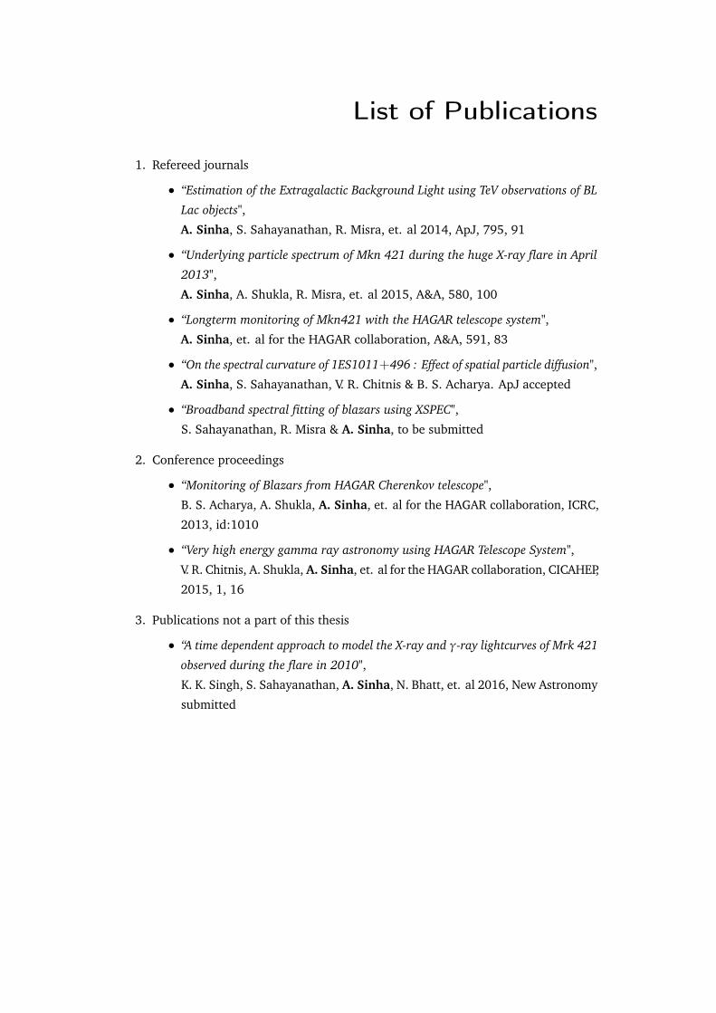
1. Refereed journals
• “Estimation of the Extragalactic Background Light using TeV observations of BL
Lac objects",
A. Sinha, S. Sahayanathan, R. Misra, et. al 2014, ApJ, 795, 91
• “Underlying particle spectrum of Mkn 421 during the huge X-ray flare in April
2013",
A. Sinha, A. Shukla, R. Misra, et. al 2015, A&A, 580, 100
• “Longterm monitoring of Mkn421 with the HAGAR telescope system",
A. Sinha, et. al for the HAGAR collaboration, A&A, 591, 83
• “On the spectral curvature of 1ES1011+496 : Effect of spatial particle diffusion",
A. Sinha, S. Sahayanathan, V. R. Chitnis & B. S. Acharya. ApJ accepted
• “Broadband spectral fitting of blazars using XSPEC",
S. Sahayanathan, R. Misra & A. Sinha, to be submitted
2. Conference proceedings
• “Monitoring of Blazars from HAGAR Cherenkov telescope",
B. S. Acharya, A. Shukla, A. Sinha, et. al for the HAGAR collaboration, ICRC,
2013, id:1010
• “Very high energy gamma ray astronomy using HAGAR Telescope System",
V. R. Chitnis, A. Shukla, A. Sinha, et. al for the HAGAR collaboration, CICAHEP,
2015, 1, 16
3. Publications not a part of this thesis
• “A time dependent approach to model the X-ray and γ-ray lightcurves of Mrk 421
observed during the flare in 2010",
K. K. Singh, S. Sahayanathan, A. Sinha, N. Bhatt, et. al 2016, New Astronomy
submitted


Contents
0 Synopsis vii
0.1 Introduction vii
0.2 Motivation and Aims ix
0.3 Methodology x
0.4 Results xi
0.4.1 Longterm study of Mkn 421 xi
0.4.2 Study of Mkn 421 during giant X-ray flare xii
0.4.3 Multi-epoch multi-wavelength study of 1ES 1011+496 xii
0.4.4 EBL estimation from VHE observations xiii
0.5 Conclusion xiv
0.6 Future prospects xv
1 Introduction: Blazars in the high energy Universe 1
1.1 AGN classification and morphology 1
1.1.1 The AGN Zoo and the unified model 2
1.1.2 Blazars 6
1.2 The Atmospheric Cherenkov Technique 9
1.2.1 Cherenkov radiation 9
1.2.2 Extensive Air Showers 10
1.2.3 Detection techniques 13
1.2.4 The TeV sky 14
1.3 Radiative mechanisms 15
1.3.1 Electromagnetic Processes 15
1.3.2 Hadronic Processes 21
1.4 Blazars emission models 22
1.4.1 Leptonic models 22
1.4.2 Hadronic models 24
1.5 Open questions about AGN jets 24
1.5.1 Jet formation 25
1.5.2 Jet propagation and acceleration 25
1.5.3 Questions specific to blazars 26
1.6 Aim of this thesis 26
2 The HAGAR Telescope Array 29
1
Contents
2.1 The Telescope Array: Design and Instrumentation 29
2.2 Data Acquisition system (DAQ) 31
2.3 Observations 33
2.4 Simulations 36
2.4.1 Performance parameters 37
2.5 Data Reduction and Analysis 38
2.5.1 Space Angle Estimation 38
2.5.2 Data Selection 41
2.5.3 Signal Extraction 42
2.6 Results 42
3 Multiwavelength Instrumentation and Data Analysis 45
3.1 Fermi-LAT 45
3.2 NuSTAR 47
3.3 Swift 48
3.3.1 Swift-BAT 49
3.3.2 Swift-XRT 49
3.3.3 Swift-UVOT 51
3.4 MAXI 52
3.5 CCD-SPOL 53
3.6 OVRO 53
4 Mkn 421: Longterm spectral and temporal study 55
4.1 Brief review of past results 55
4.2 Data Analysis 58
4.2.1 HAGAR 58
4.2.2 Other multiwavelength data 59
4.3 Multiwavelength temporal study 60
4.3.1 Variability and correlations 61
4.3.2 Detection of lognormality 65
4.4 Spectral modelling 65
4.5 Results and discussions 73
4.5.1 Spectral variability 73
4.5.2 Location of the emission zone 74
4.5.3 Implications of lognormality 75
4.6 Conclusions 76
5 Mkn 421: Underlying particle spectrum during giant flare 77
5.1 Behaviour during previous flares 77
5.2 Multiwavelength observations and data analysis 78
5.3 Multiwavelength temporal study 80
2
5.4 X-ray spectral analysis 82
5.4.1 Fitting the photon spectrum 84
5.4.2 Emitting particle distribution 85
5.5 Discussions:Evidence of multicomponent emission 90
5.6 Conclusions 92
6 1ES 1011+496: Effect of spatial particle diffusion on spectral curvature 93
6.1 Introduction 93
6.2 Data analysis and lightcurves 94
6.3 Temporal Analysis: Detection of Lognormality 97
6.4 Spectral Energy Distribution 97
6.5 Electron escape and spectral curvatures 102
6.5.1 Analytic solution: Thomson scattering 104
6.5.2 Numerical solution: Klein-Nishina scattering 104
6.6 Conclusions 105
7 The Extragalactic Background Light: Estimation using TeV observations 109
7.1 Introduction 109
7.2 EBL estimation from VHE observation 111
7.2.1 Interaction of VHE photons with the EBL 112
7.2.2 EBL estimates computed from VHE observations 112
7.3 Statistical signature on VHE spectra of blazars 115
7.4 EBL Estimation 117
7.5 Implications of the estimated spectrum 122
7.5.1 Comparison with other estimations 122
7.5.2 Consistency with blazar radiative models 125
7.5.3 The Gamma Ray Horizon 125
7.6 Conclusions 126
8 Conclusions: A summary and the way forward 131
8.1 Summary of thesis 131
8.2 Future plans 133
Appendices 139
A XSPEC implementaion of SSC 141
A.1 Obtaining approximate guess values of physical parameters 141
A.2 XSPEC Spectral fit 144
B A Few Acronyms 147
Bibliography 169
3

List of Tables
Table 2.1 Observations of extragalactic sources with HAGAR 43
Table 3.1 Swift-UVOT filter characteristics 52
Table 4.1 HAGAR observation details for different epochs 59
Table 4.2 X-ray and GeV spectral parameters during various epochs 60
Table 4.3 Fractional variability Fvar at different wavebands 63
Table 4.4 Detection of lognormality 68
Table 4.5 Fit parameters for the different SED states 73
Table 5.1 Details of NuSTAR pointings 79
Table 5.2 Details of Swift pointings 79
Table 5.3 Frms at different frequencies during X-ray flare. 82
Table 5.4 Reduced χ2 values for the photon spectrum 85
Table 5.5 Fit parameters of the log parabolic photon spectrum 86
Table 5.6 Reduced χ2 for the various particle distributions 89
Table 5.7 Sample parameters of the best fit model for the photon and
particle spectrum 89
Table 5.8 The best fit parameters for the LP particle distribution 89
Table 6.1 Spectral details of different epochs 95
Table 6.2 Models parameters for different particle spectra 103
Table 7.1 List of HBLs detected at VHE 116
List of Figures
Figure 1.1 Basic structure of AGN 3
Figure 1.2 AGN classification scheme 3
Figure 1.3 Multiwavelength image of Cygnus A 5
Figure 1.4 Unified AGN model 6
Figure 1.5 Typical double hump SED of blazars 8
Figure 1.6 The blazar sequence 8
Figure 1.7 Polarisation in dielectric medium 11
Figure 1.8 Toy model of EAS 12
4

List of Figures
Figure 1.9 Schematic differences between photon and hadron showers 12
Figure 1.10 Lateral distribution of photon and hadron showers 13
Figure 1.11 The VHE sky 14
Figure 1.12 Synchrotron spectrum 17
Figure 1.13 Synchrotron self absorption spectrum 18
Figure 1.14 Inverse Compton cross-section 20
Figure 1.15 Bremsstrahlung spectrum 21
Figure 1.16 Leptonic and hadronic SED models 25
Figure 2.1 The HAGAR Telescope Array. 30
Figure 2.2 Schematic layout of the the HAGAR Array. 30
Figure 2.3 Bright Star Scan 32
Figure 2.4 Pointing offset for HAGAR mirrors 32
Figure 2.5 Rate-threshold plot 34
Figure 2.6 HAGAR Telescope Electronics 34
Figure 2.7 HAGAR Trigger Set-up 35
Figure 2.8 HAGAR observation duration 36
Figure 2.9 HAGAR differential rate plots 38
Figure 2.10 HAGAR significance plot 39
Figure 2.11 Arrival time reconstruction 41
Figure 2.12 Space angle distribution 43
Figure 3.1 Schematic of the LAT telescope 46
Figure 3.2 Fermi-LAT counts map of Mkn421 46
Figure 3.3 Schematic of the NuSTAR telescope 47
Figure 3.4 NuSTAR image of Mkn421 48
Figure 3.5 Schematic of the Swift telescope 49
Figure 3.6 Swift-XRT operating mode images 50
Figure 3.7 Pileup estimation in Swift-XRT 51
Figure 3.8 Pileup exclusion in Swift-XRT 51
Figure 3.9 Swift-UVOT image of BL Lac 52
Figure 4.1 Historical VHE lightcurve of Mkn 421 56
Figure 4.2 Radio image of Mkn 421 57
Figure 4.3 Optical image of Mkn 421 57
Figure 4.4 HAGAR lightcurve for Mkn 421 58
Figure 4.5 Multiwavelength light curve of Mkn421 from 2009-2015 62
Figure 4.6 Fractional variability Fvar at different wavebands 63
Figure 4.7 Hardness ratio in the X-ray and GeV bands 63
Figure 4.8 z-DCF between the various wavebands 64
Figure 4.9 Histogram of flux distribution 66
Figure 4.10 Flux-rms scatter plots 67
Figure 4.11 Mkn 421 R-band flux distribution 68
Figure 4.12 SED during different states fit with SSC model 72
5

List of Figures
Figure 4.13 Cross plot of the fit parameters for the one-zone SSC 74
Figure 4.14 Origin of lag between radio and γ-ray flares 74
Figure 4.15 Observation bias in pointing instruments 75
Figure 5.1 Flux brightening during April 2013 80
Figure 5.2 Multiwavelength light curve during April 2013 flare 81
Figure 5.3 Computed z-DCF with NuSTAR data 83
Figure 5.4 Hardness ratio during April 2013 flare 83
Figure 5.5 Time bins for which spectral fitting 84
Figure 5.6 Cross plot of parameters for the logparabolic photon and particle
spectrum 86
Figure 5.7 Cross plot of the two indices of the broken power-law particle
spectrum 88
Figure 5.8 Observed X-ray and UV spectrum during two states. 90
Figure 5.9 Fitted spectrum and residuals for the three spectral models 91
Figure 6.1 Redshift measurement of 1ES 1011+496 94
Figure 6.2 Published TeV spectrum and SED of 1ES 1011+496 95
Figure 6.3 Longterm Fermi-LAT spectrum and extracted SEDs 98
Figure 6.4 Multiwavelength lightcurve of 1ES 1011+496 99
Figure 6.5 Detection of lognormality in 1ES 1011+49 100
Figure 6.6 SEDs modelled with CPL and SBPL 102
Figure 6.7 Comparison of different particle spectra 103
Figure 6.8 Difference between the Thomson condition and KN condition 105
Figure 6.9 Effect of energy dependence of the escape time scale on final
spectrum 106
Figure 6.10 Particle spectra obtained for ξ= −0.7 106
Figure 7.1 Background radiation in the universe 110
Figure 7.2 Observational limits on the EBL intensity. 111
Figure 7.3 Variation in different EBL models 112
Figure 7.4 Schematic illustration of the γ−γ pair production 113
Figure 7.5 The cross section for the γ−γ interaction 113
Figure 7.6 Limits on the EBL as determined from γ−ray observations of
blazars 114
Figure 7.7 Distribution of the observed VHE spectral index with redshift 118
Figure 7.8 Distribution of the observed X-ray spectral index with redshift 118
Figure 7.9 Distribution of the observed Fermi-LAT spectral index with red-
shift and luminosity 119
Figure 7.10 Distribution of the observed VHE spectral index with luminos-
ity 119
Figure 7.11 EBL spectrum estimated in this work. 122
Figure 7.12 Parameter space for k and εp 123
6
List of Figures
Figure 7.13 Validity of the estimated EBL within radiative transfer mod-
els 126
Figure 7.14 The Gamma Ray Horizon 127
Figure 7.15 Exponential turnover in the absorption corrected VHE spectra of
distant sources. 128
Figure 8.1 AstroSat simulations of HBLs 134
Figure 8.2 Status of the MACE telescope 135
Figure 8.3 Sensitivity plot for CTA 136
Figure A.1 Comparison between analytical and numerical solutions for SSC
and EC 143
Figure A.2 XSPEC module fit to SED of 3C 279 145
0

“It doesn’t matter how beautiful your theory is, it doesn’t
matter how smart you are. If it doesn’t agree with experi-
ments, it’s wrong."
Richard P. Feynman
1Introduction: Blazars in the high
energy Universe
OUT OF THE BILLIONS of galaxies in our Universe, a small fraction (∼ 5%) has a very
active nucleus - a small region (∼ light days) at the center of the galaxy, which outshines
the total emission from the remaining of the host galaxy. These galaxies have total
luminosity exceeding 1044 ergs/s, and are termed as active galactic nuclei (AGN). In
contrast to the energy spectrum from normal galaxies (a blackbody), AGNs have a broad
energy spectrum extending from radio to beyond X-ray energies. Around 10-15% of the
AGNs are radio-loud, and observationally exhibit prominent bipolar radio jets reaching
up to Mpc scales. According to the unified AGN model of Urry & Padovani (1995), blazars
are radio-loud AGNs with one of the jets aligned at a close angle to our line of sight.
Blazars are the most prominent objects seen at very high energies (VHE; > 100 GeV). In
this chapter, we review our present understanding of blazars and address some of the
open questions in the field, with emphasis on VHE emission and detection techniques.
1.1 A G N C L A S S I F I CAT I O N A N D M O R P H O L O GY
By the end of the 1950s, synchrotron emission was well established to be the dominant
process for the radio emission from extragalactic radio sources. Burbidge (1959) used
this to show that the minimum energy content of AGNs is extremely large ∼ 1060 ergs,
and attributed this large energy to a chain of supernovae explosions occurring in a tightly
packed set of stars at the nuclear region of the galaxy. Hoyle & Fowler (1963a,b) showed
in their pioneering papers that such close packed stars can as well form a single super
massive object, and that the energy of the radio sources was of gravitational origin derived
from the slow contraction of a super massive object under its own strong gravitational
1

1. Introduction: Blazars in the high energy Universe
field. This idea was further developed by many authors (eg; Salpeter (1964); Shakura &
Sunyaev (1973); Lynden-Bell (1969)), and we now believe that AGNs host a supermassive
black hole (∼ 106−109Msun ) at their center, and as matter is attracted by the black hole
gravity, it is compressed, heated, and then it radiates.
The development of our understanding of AGNs, observations and theory, is a fasci-
nating read, and can be found in the books by Schmidt (1990) and Krolik (1999). Here,
we only outline the basic structure of AGNs (Figure 1.1) as we currently understand
(Ghisellini, 2013):
• A supermassive blackhole at the center, which acts as the central engine.
• An accretion disk, formed by matter spiralling into the central black hole. This is
understood to be the major source of power in the jet.
• An X-ray corona, sandwiching the accretion disk. It is supposed to be a hot layer,
or an ensemble of clumpy regions particularly active in the inner parts of the disk.
• An obscuring torus located at several parsec from the black hole, intercepting
some fraction of the radiation produced by the disk and re-emitting it in the
infrared.
• Broad Line Regions (BLR), regions of many small and dense (n(H) ∼ 1010 cm−3)
clouds at a distance of ∼ 1 pc from the black hole moving rapidly (∼ 3000 km/s).
They intercept ∼10% of the ionizing radiation of the disk, and re-emit it in the
form of lines, which are broadened due to Doppler shifts.
• Narrow Line Regions (NLR), which are regions of less dense clouds (∼ 103 cm−3)
moving less rapidly (n(H) ∼ 300 km/s) as compared to BLR.
• Relativistic, bipolar radio jets characterized by a non-thermal broadband emis-
sion.
1.1.1 The AGN Zoo and the unified model
AGNs emit spectacularly over the entire accessible electromagnetic spectrum and thus
have been one of the main sources in any new window of the electromagnetic spectrum
resulting from the technological advances in instrumentation. This has led to many
different and independent classification schemes (Figure 1.2) in different energy bands
e.g optical morphology, radio morphology, variability, luminosity etc. (Tadhunter, 2008);
making the AGN classification complex and often confusing.
• Based on radio emission, AGNs are broadly classified into two groups, namely,
radio-loud and radio-quiet. Sources with the ratio of emission at the 5 GHz to
2

1.1. AGN classification and morphology
Figure 1.1.: Basic morphology of AGNs (according to the classification scheme of Urry &Padovani (1995).
Figure 1.2.: The AGN zoo showing the different classes of AGNs.
3

1. Introduction: Blazars in the high energy Universe
emission in the optical B-band greater than 10 have been termed as radio-loud,
others radio-quiet. Though the first quasars that were discovered were radio-loud,
we now know that these radio-loud AGNs constitute roughly 10% of all AGNs, with
the majority being radio-quiet. Observationally, radio-loud AGNs are distinctly
characterized by highly relativistic bipolar radio jets reaching up to Mpc scales,
and are generally more powerful than their radio-quiet counterparts.
Radio-quiet AGNs include Seyferts, galaxies which show a bright star-like nucleus
with very high surface brightness and strong, high-ionization lines in their optical-
UV spectra. They are further subdivided into Seyfert 1 or Seyfert 2 according
to whether their optical spectra show both broad and narrow emission lines or
only narrow emission lines. These are mainly spiral galaxies and are radio-quiet.
However, a particular subclass known as Narrow Line Seyfert Galaxies is now
known to be radio-loud and shows a rapid and large variation across the entire
accessible electromagnetic spectrum similar to blazars. Quasars, characterized by
a blue bump due to excess UV emission, may be both radio-loud and radio-quiet.
Radio Galaxies (radio-loud AGNs) show a bright star-like nucleus in optical but
a non-stellar continuum and an extended structure in radio emission exhibiting
core-jet morphology. The relativistic bipolar jets are often symmetrical on either
side of the active nucleus. They are further subdivided into Broad Line Radio
Galaxies and Narrow Line Radio Galaxies depending on whether their optical
spectra show both broad and narrow emission lines or only narrow emission lines,
which are further subdivided morphologically according to their appearance in
radio images as Fanaroff Riley I (FR I) and Fanaroff Riley II (FR II) (Fanaroff &
Riley, 1974). FR I have jets that become fainter and fainter as one moves away
from the central engine. Due to this feature they are also known as edge-darkened
sources. On the other hand, FR II are edge-brightened sources where jets become
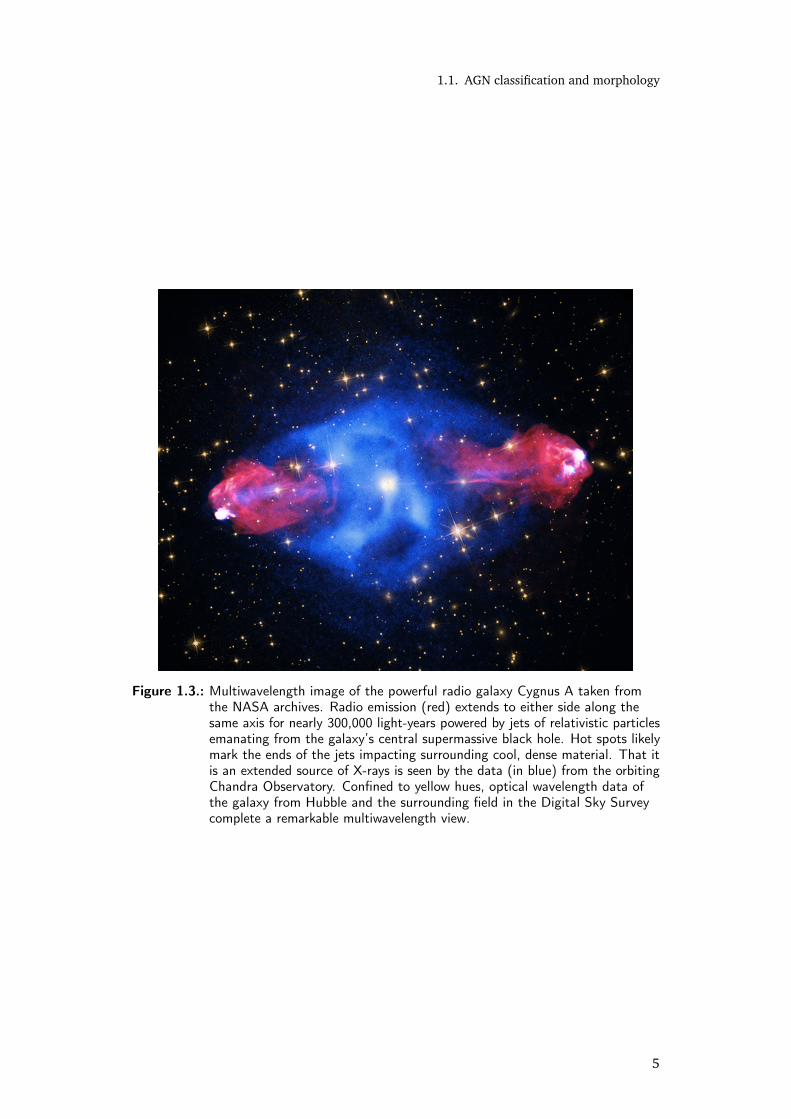
fainter towards the central engine. Figure 1.3 shows a composite radio, optical and
X-ray image of the powerful radio galaxy Cygnus A, showing the edge brightened
radio jets, the X-ray corona and the host galaxy.
• Based on Optical/UV Spectroscopy, AGNs are subdivided on the basis of strength
and nature of their observed optical-UV emission lines. Those exhibiting strong,
broad, as well as narrow emission-lines have been classified as Type-1 AGN while
sources with only narrow emission lines are known as Type-2 AGNs.
The AGN unification model, first proposed by Antonucci (1984) and later developed
by several authors (see Netzer (2015) and references therein) assumes that the physics
of all the AGNs are same and the observed differences between different classes are only
due to their relative orientation with respect to the line of sight (Figure 1.4). It is mainly
based on three fundamental pillars: orientation, covering factor and luminosity. The
main elements responsible for different realizations are the axis-symmetric dust clouds
known as the torus and the bipolar relativistic jets in case of radio-loud sources. The
4
1.1. AGN classification and morphology
Figure 1.3.: Multiwavelength image of the powerful radio galaxy Cygnus A taken fromthe NASA archives. Radio emission (red) extends to either side along thesame axis for nearly 300,000 light-years powered by jets of relativistic particlesemanating from the galaxy’s central supermassive black hole. Hot spots likelymark the ends of the jets impacting surrounding cool, dense material. That itis an extended source of X-rays is seen by the data (in blue) from the orbitingChandra Observatory. Confined to yellow hues, optical wavelength data ofthe galaxy from Hubble and the surrounding field in the Digital Sky Surveycomplete a remarkable multiwavelength view.
5

1. Introduction: Blazars in the high energy Universe
unification within radio-quiet counterparts requires only the torus while the radio-loud
counterparts requires both the torus and the bipolar jets. The integration of radio-loud
and radio-quiet under one family “AGNs" requires both the anisotropic components and
Doppler boosting. Thus in radio-quiet AGNs, Seyfert 1 is the one where the view of the
central engine is not blocked by the torus while the converse is true in case of Seyfert 2.
Figure 1.4.: An artist impression of the unified AGN model taken from Beckmann &Shrader (2012b). The core of the diagram shows all the possible componentsthat constitute an AGN (not to scale). The outer part depicts the manifesta-tion of AGN depending on our viewing angle to the source.
1.1.2 Blazars
Blazars count among the most violent sources of high energy emission in the known
universe, observationally characterized by:
• A highly variable nonthermal emission across the entire electromagnetic spectrum
• A typical double hump broadband spectral energy distribution (SED), with one in
the IR - X-ray regime, and the second one in the γ-ray regime
• Variability at all time scales, from hours to years
• Strong radio and optical polarization
• Apparent superluminal motion in high resolution radio maps
According to the classification scheme of Urry & Padovani (1995), the likely explanation
of such observations is that they are a subclass of radio-loud AGNs where the relativistic
jet is oriented close to the line of sight. The observed properties are believed to be a
6

1.1. AGN classification and morphology
manifestation of relativistic aberration associated with relativistic bulk motion of plasma
at small angles to our line of sight, resulting in Doppler boosting of flux, frequency, and
temporal characteristics. The relativistic bulk motion is duly attested by the ubiquity
of superluminal motion, one-sided morphologies, γ-ray transparency and intra-day
variability in the radio wavebands.
Based on the rest frame equivalent width of their emission lines in optical/UV spectra,
blazars have been further classified in two subgroups: BL Lacertae objects (BL Lacs)
with very weak/no emission lines and Flat Spectrum Radio Quasars (FSRQ) with strong
broad-line emission. In terms of radiative output, BL Lacs belong to the low luminosity
class of blazars and are thought to be FR I sources in the AGN unification scheme (Urry
& Padovani, 1995; Tadhunter, 2008), while FSRQs are more powerful and are believed
to be the FR II counterparts.
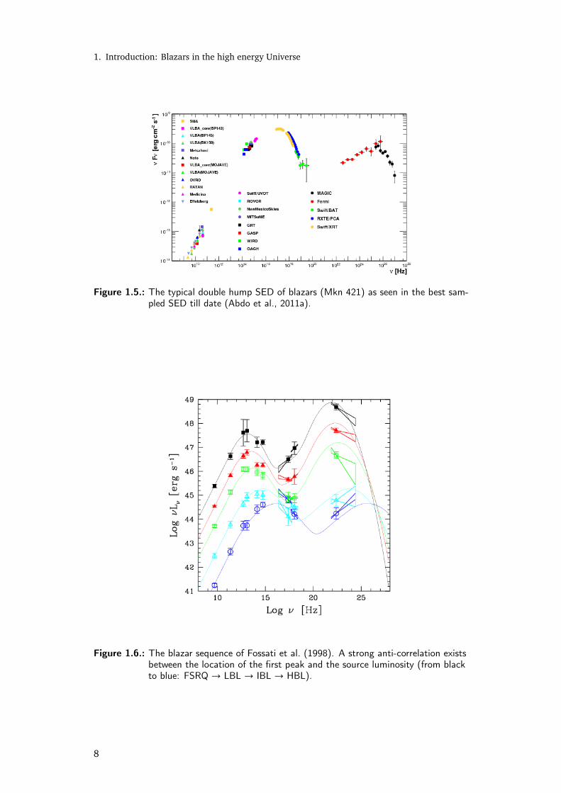
The broad-bimodal SED (Figure 1.5) is one of the unique characteristics of blazars.
Except for few cases, the broadband SED is fully non-thermal with two broad components
peaking between well defined energy ranges. According to the location of the first peak
(νp), BL Lacs are further classified into low-energy peaked BL Lacs (LBL; νp < 1014
Hz), intermediate peaked BL Lacs (IBL; 1014 < νp < 1015 Hz ) and high-energy peaked
BL Lacs (HBL; νp > 1015 Hz) (Padovani & Giommi, 1995).The two humps also exhibit
a tight anti-correlation between the source bolometric luminosity and location of the
peak of the low energy hump in the average SED of blazars (Figure 1.6). In addition
to this, anti-correlation has also been found between the low-energy-hump peak with
the luminosity of the low-energy-hump as well as with the γ-ray dominance. These
correlations were termed as evidence for a “blazar sequence" (Fossati et al., 1998) - an
apparent continuous spectral trend from luminous, low-energy-peaked, γ-ray dominant
sources with prominent broad emission lines to a less luminous high-energy-peaked
sources with very weak or no emission lines. Since its proposal, the blazar sequence has
been observationally and phenomenologically studied in depth by various authors, with
roughly similar conclusions [eg: Giommi et al. (2012); Ghisellini et al. (2009); Ghisellini
& Tavecchio (2008); Nieppola et al. (2006); Antón & Browne (2005); Ghisellini (2016)].
The first significant detection of extragalactic TeV photons from the blazar Mkn 421 by
the Whipple collaboration in 1992 (Punch et al., 1992) using the Atmospheric Cherenkov
Technique has given us new clues, and and unfolded new mysteries behind the workings
of these objects. Detection at TeV energies is particularly challenging because
1. The flux of photons falls off steeply at these energies, dNdE ∼ E−α, where α ∼ 3.
This implies very poor statistics, and large integration time of telescopes with large
effective areas are required.
2. TeV photons from distant galaxies interact with the optical/UV photons of the
extragalactic background light (EBL) and suffer attenuation (thus further steepening
the index) and spectral distortion.
7
1. Introduction: Blazars in the high energy Universe
Figure 1.5.: The typical double hump SED of blazars (Mkn 421) as seen in the best sam-pled SED till date (Abdo et al., 2011a).
Figure 1.6.: The blazar sequence of Fossati et al. (1998). A strong anti-correlation existsbetween the location of the first peak and the source luminosity (from blackto blue: FSRQ → LBL → IBL → HBL).
8

1.2. The Atmospheric Cherenkov Technique
3. The Atmosphere is opaque to γ-rays, and these photons have to be indirectly
detected through the induced air showers. Reconstructing the initial energy and
direction of the primary γ-ray requires the use of extensive Monte Carlo simulations
and novel techniques which we describe in the next section.
1.2 T H E AT M O S P H E R I C C H E R E N KOV T E C H N I Q U E
In 1952, a new window was opened on our universe when Galbraith and Jelly detected
brief flashes of light in the night-sky using an ex-wartime parabolic signalling mirror
clamped with a small photomultiplier tube at the focus on a free running oscilloscope
at the Extensive Air Shower (EAS) array experiment at UK Atomic Energy Research
Establishment in Oxfordshire (Galbraith & Jelley, 1953). Over several nights, they
confirmed a correlation between signals from the array and the detected short duration
(∼ 100 ns) pulses. This confirmed Blackett’s suggestion that cosmic rays, and hence also
gamma rays, contribute to the light intensity of the night sky via the Cherenkov radiation
produced by the air showers that they induce in the atmosphere. However, it took a long
and frustrating wait of more than 25 years before the first detection of a TeV source - the
Crab Nebula at 5σ by the Whipple Telescope (Weekes et al., 1989). An engrossing history
of the development of this field can be found in the review article by Hillas (2013).
1.2.1 Cherenkov radiation
Cherenkov radiation is an electromagnetic radiation emitted when a charged particle
(such as an electron) passes through a dielectric medium at a speed greater than the
phase velocity of light in that medium. Cherenkov radiation was first observed by Marie
Curie in the year 1910 as a bluish glow from bottles containing radioactive radium salts
dissolved in liquids. However, she attributed this to some kind of luminescence, and it
took a series of experiments by Cherenkov and Vavilov between the years 1934 to 1937
to understand the nature of this radiation.
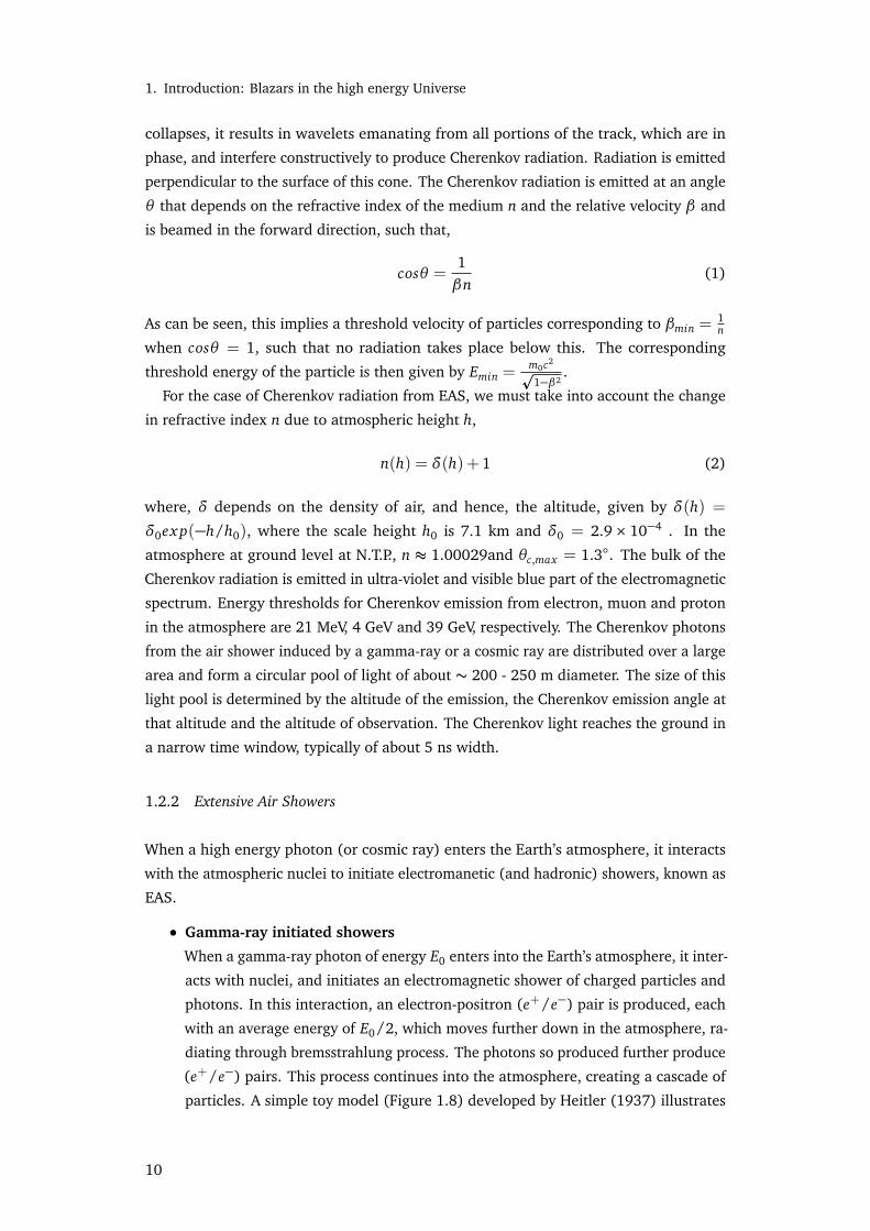
When a charged particle of mass m0 is moving in a dielectric medium, the electric
field of the particle distorts the atoms in the vicinity of its track, resulting in induced
dipole moments of the atoms. When the particle moves to another point, the elongated
atoms along the initial point, say P, return to their original configuration, which is
accompanied by the emission of an electric pulse. For slow moving particles (v < cm,
where cm is the phase velocity of light in the medium), the polarization is more or less
symmetrical w.r.t particle position, as shown in panel (a) of Figure 1.7, resulting in no
net electric field at long distances due to destructive interference and thus, no radiation.
However, for particles with v > cm, the polarization is no longer symmetrical along the
planes in the trajectory of the particle (panel (b) of Figure 1.7). Thus, a cone of dipoles
develops behind the charged particle, creating a distinct dipole field. When this state
9
1. Introduction: Blazars in the high energy Universe
collapses, it results in wavelets emanating from all portions of the track, which are in
phase, and interfere constructively to produce Cherenkov radiation. Radiation is emitted
perpendicular to the surface of this cone. The Cherenkov radiation is emitted at an angle
θ that depends on the refractive index of the medium n and the relative velocity β and
is beamed in the forward direction, such that,
cosθ =1βn
(1)
As can be seen, this implies a threshold velocity of particles corresponding to βmin =1n
when cosθ = 1, such that no radiation takes place below this. The corresponding
threshold energy of the particle is then given by Emin =m0c2p
1−β2.
For the case of Cherenkov radiation from EAS, we must take into account the change
in refractive index n due to atmospheric height h,
n(h) = δ(h)+ 1 (2)
where, δ depends on the density of air, and hence, the altitude, given by δ(h) =
δ0ex p(−h/h0), where the scale height h0 is 7.1 km and δ0 = 2.9× 10⁻⁴ . In the
atmosphere at ground level at N.T.P., n ≈ 1.00029and θc,max = 1.3. The bulk of the
Cherenkov radiation is emitted in ultra-violet and visible blue part of the electromagnetic
spectrum. Energy thresholds for Cherenkov emission from electron, muon and proton
in the atmosphere are 21 MeV, 4 GeV and 39 GeV, respectively. The Cherenkov photons
from the air shower induced by a gamma-ray or a cosmic ray are distributed over a large
area and form a circular pool of light of about ∼ 200 - 250 m diameter. The size of this
light pool is determined by the altitude of the emission, the Cherenkov emission angle at
that altitude and the altitude of observation. The Cherenkov light reaches the ground in
a narrow time window, typically of about 5 ns width.
1.2.2 Extensive Air Showers
When a high energy photon (or cosmic ray) enters the Earth’s atmosphere, it interacts
with the atmospheric nuclei to initiate electromanetic (and hadronic) showers, known as
EAS.
• Gamma-ray initiated showers
When a gamma-ray photon of energy E0 enters into the Earth’s atmosphere, it inter-
acts with nuclei, and initiates an electromagnetic shower of charged particles and
photons. In this interaction, an electron-positron (e+/e−) pair is produced, each
with an average energy of E0/2, which moves further down in the atmosphere, ra-
diating through bremsstrahlung process. The photons so produced further produce
(e+/e−) pairs. This process continues into the atmosphere, creating a cascade of
particles. A simple toy model (Figure 1.8) developed by Heitler (1937) illustrates
10
1.2. The Atmospheric Cherenkov Technique
Figure 1.7.: Polarization state of the medium when the velocity of the charged particleis (a) less than the phase velocity of light in that medium (v < cm) and (b)greater than the phase velocity of light in that medium (v > cm).
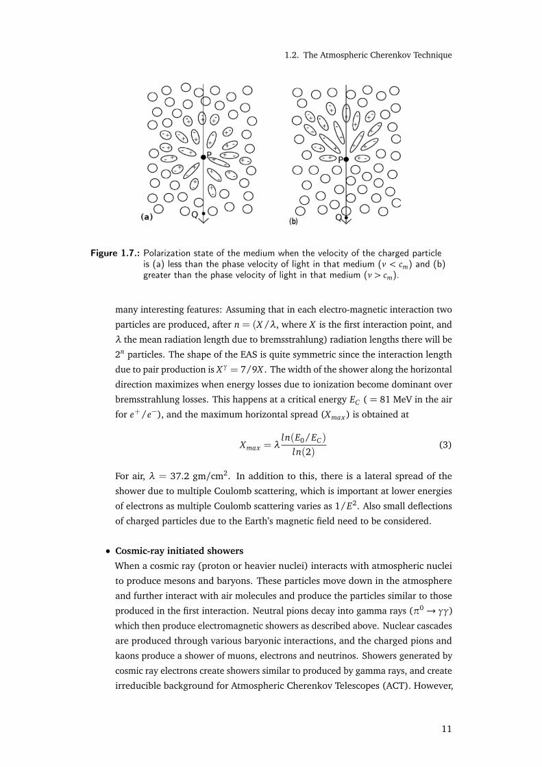
many interesting features: Assuming that in each electro-magnetic interaction two
particles are produced, after n = (X /λ, where X is the first interaction point, and
λ the mean radiation length due to bremsstrahlung) radiation lengths there will be
2n particles. The shape of the EAS is quite symmetric since the interaction length
due to pair production is X γ = 7/9X . The width of the shower along the horizontal
direction maximizes when energy losses due to ionization become dominant over
bremsstrahlung losses. This happens at a critical energy EC ( = 81 MeV in the air
for e+/e−), and the maximum horizontal spread (Xmax) is obtained at
Xmax = λln(E0/EC )
ln(2)(3)
For air, λ = 37.2 gm/cm2. In addition to this, there is a lateral spread of the
shower due to multiple Coulomb scattering, which is important at lower energies
of electrons as multiple Coulomb scattering varies as 1/E2. Also small deflections
of charged particles due to the Earth’s magnetic field need to be considered.
• Cosmic-ray initiated showers
When a cosmic ray (proton or heavier nuclei) interacts with atmospheric nuclei
to produce mesons and baryons. These particles move down in the atmosphere
and further interact with air molecules and produce the particles similar to those
produced in the first interaction. Neutral pions decay into gamma rays (π0→ γγ)
which then produce electromagnetic showers as described above. Nuclear cascades
are produced through various baryonic interactions, and the charged pions and
kaons produce a shower of muons, electrons and neutrinos. Showers generated by
cosmic ray electrons create showers similar to produced by gamma rays, and create
irreducible background for Atmospheric Cherenkov Telescopes (ACT). However,
11

1. Introduction: Blazars in the high energy Universe
since the flux of cosmic ray electrons is low and falls rapidly with energy, the
electron background is not very significant above 100 GeV.
Figure 1.8.: Toy model of Heitler (1937) to explain EAS in atmosphere.
Figure 1.9 shows a schematic diagram of photon (electromagnetic only) and cosmic-ray
(electromagnetic, muonic and hadronic) induced cascades. Hadronic showers, consisting
of many sub-shower profiles, show more fluctuations in their timing profile as compared
to photon showers, and while the lateral shower profile of photon showers show a typical
hump (Figure 1.10) due to artificial focussing of Cherenkov light, the same is wiped out
in hadronic showers due to the fluctuations.
Figure 1.9.: Schematic differences between photon (left) and hadron (right) induced show-ers, taken from Mankuzhiyil (2010).
12

1.2. The Atmospheric Cherenkov Technique
Figure 1.10.: Lateral distribution of Cherenkov photons on ground for γ and hadronicshowers as obtained from simulations (Fegan, 1997).
1.2.3 Detection techniques
The Cherenkov emission produced by EAS is coherent and it can be detected by an array
of optical detectors on the ground by using ACT against the night sky background (NSB)
and ambient light. Gamma-ray astronomy at the highest energies, (at ∼ above 100 GeV),
is performed through this technique.
1.2.3.1 Wavefront sampling Technique
The Cherenkov photons from EAS create a light cone on the ground, which are collected
by optical reflectors with a PMT at the focal point of each reflector. These photons are
sampled from different locations of the Cherenkov light pool. Therefore, an array of
detectors separated by distances in the range of 10 m to 100 m is required to collect
Cherenkov photons in coincidence. The arrival direction of the shower is determined
by the relative time of arrival of the Cherenkov shower front at the individual detectors.
Previous experiments like Themistocle and CELESTE in France, Solar Tower Atmospheric
Cherenkov Effect Experiment (STACEE) in USA and Pachmarhi Array of Cherenkov
Telescopes (PACT) in India, and currently the HAGAR Telescope array (see Chapter 2) in
India made use of this technique.
13
1. Introduction: Blazars in the high energy Universe
1.2.3.2 Imaging Technique
Imaging Atmospheric Cherenkov Technique is the most powerful way of detecting VHE
photons. Imaging Air Cherenkov Telescope (IACT) collects the Cherenkov photons on
its large mirror surface, and points them on a camera kept in the focal plane. The
camera consists of PMTs to convert the photons into electric signal. The recorded event
is the geometrical projection of atmospheric showers. Cherenkov photons emitted at
different heights form images at different positions of the camera. The image contains
the information of longitudinal development of EAS from the number of photons and
arrival time of the images. When the telescope is pointed towards a VHE source on the
sky, images are formed near the camera center by the upper part of the shower, where
the secondary particles are more energetic. The images of the photons from the lower
part of the shower are formed away from the center of the camera. The direction and
energy of the primary photons are reconstructed from the shower images.
This technique was pioneered by the Whipple Telescope (Weekes et al., 1989), and later
on by the High-Energy-Gamma-Ray Astronomy (HEGRA) at La Palma and is currently used
by the Very Energetic Radiation Imaging Telescope Array System (VERITAS), High Energy
Stereoscopic System (HESS) and Major Atmospheric Gamma-ray Imaging Cherenkov
Telescope (MAGIC) Telescopes.
1.2.4 The TeV sky
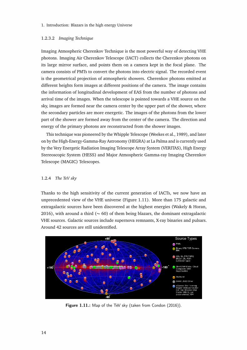
Thanks to the high sensitivity of the current generation of IACTs, we now have an
unprecedented view of the VHE universe (Figure 1.11). More than 175 galactic and
extragalactic sources have been discovered at the highest energies (Wakely & Horan,
2016), with around a third (∼ 60) of them being blazars, the dominant extragalactic
VHE sources. Galactic sources include supernova remnants, X-ray binaries and pulsars.
Around 42 sources are still unidentified.
Figure 1.11.: Map of the TeV sky (taken from Condon (2016)).
14

1.3. Radiative mechanisms
1.3 R A D I AT I V E M E C H A N I S M S
In this section, we briefly mention the major sources of continuum radiation incurred in
astrophysical situations.
1.3.1 Electromagnetic Processes
Most of the observed radiation comes from electromagnetic losses incurred by electrons
and positrons in astrophysical plasmas. Excellent descriptions of these phenomena can
be found in Blumenthal & Gould (1970); Rybicki & Lightman (1986); Longair (2011).
1.3.1.1 Blackbody emission
Photons emitted by matter in thermal equilibrium with radiation is known as blackbody
radiation. Such systems follow a characteristic spectrum known as Planck spectrum with
specific energy density given by
uν(Ω) =2hν3/c22
ex p( hνkB T −1)
er gs cm−3Hz−1sr−1 (4)
where ν is the emitted photon frequency, Ω the solid angle along the normal to
the emission surface, c the speed of light, h the Planck constant, kB the Boltzmann
constant and T the effective blackbody temperature. The peak photon frequency at
which the energy density is maximum for a given temperature T is given by Wien’s law,
νpeak = 2.82(kB/h)T . Integrating Equation 4 over the entire photon frequency and
the solid angle, we get the Stefan-Boltzmann law for the energy density of a blackbody
spectrum
u(T ) = aT4 (5)
where a = 4σ/c with σ the Stefan-Boltzmann constant. Any continuum emission
spectrum which cannot be accounted for by a blackbody spectrum is, usually (and in this
thesis), referred to as non-thermal spectrum. Examples of blackbody radiation include
the observed spectrum of stars and planets, and the thermal component from the host
galaxy in AGN spectra.
1.3.1.2 Synchrotron emission
Radiation emitted as a result of radial acceleration of charged particles in magnetic fields
is known as synchrotron radiation. The power radiated at frequency ν by an electron
of energy γmec2, moving at a speed of β(= v/c) in a magnetic field B at a pitch angle
(angle between magnetic field and particle velocity) of α is given by
15

1. Introduction: Blazars in the high energy Universe
P(ν,γ) =
p3e3Bsin(α)
mec2F(ν
νc) (6)
νc = 1.5γ2νLsin(α) (7)
where νL = eB/2πmec is the Larmor frequency and νc the critical frequency. The
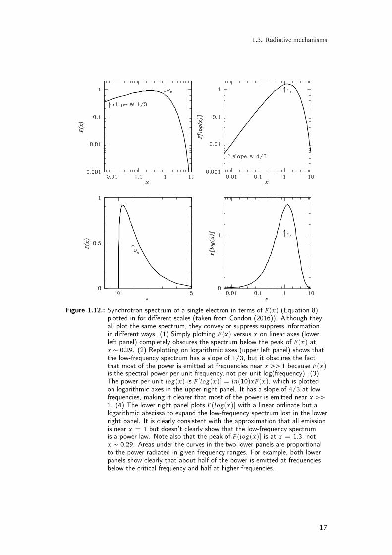
synchrotron power function, F(x) is given by
F(x) = x
∫ ∞
xK 5
3(z)dz (8)
with K 53
the modified Bessel function of fractional order 5/3. The shape of the spectrum
is governed by F(ν/νc)which peaks at ∼ 0.29(ν/νc) (Figure 1.12). The total radiated
power by an electron with a given pitch angle α can be found from Equation 7 and 8
P(γ,α) = 2cσTβ2γ2 B2
8πsin2α (9)
where σT is the Thomson scattering cross-section. For an isotropic velocity distribution,
the average power radiated per particle can be obtained by averaging over the velocity
field as
Ps yn(γ) =1
4π
∫
P(γ,α)sinαdΩ (10)
=1
8πcσTβ
2γ2B2 (11)
For an isotropic power-law electron distribution described by
N(γ) = Kγ−δ (12)
the resulting synchrotron spectrum can be shown to be a power-law with spectral index
−(δ− 1)/2. Examples include the radio emission of our galaxy, supernova remnants
and extragalactic radio sources, and the non-thermal low energy continuum of the Crab
Nebula and most quasars.
• Synchrotron Self Absorption
Relativistic charged particles, in addition to emitting synchrotron radiation, can
also get energized via absorbing the emitted synchrotron photons. This absorption
process is known as synchrotron-self absorption (SSA). This leads to the emitted
synchrotron spectrum getting modified at the low energy end. For a uniform source
without any input, the observed spectrum is given by
Iν = Sν(1− e−τν) (13)
16
1.3. Radiative mechanisms
Figure 1.12.: Synchrotron spectrum of a single electron in terms of F(x) (Equation 8)plotted in for different scales (taken from Condon (2016)). Although theyall plot the same spectrum, they convey or suppress suppress informationin different ways. (1) Simply plotting F(x) versus x on linear axes (lowerleft panel) completely obscures the spectrum below the peak of F(x) atx ∼ 0.29. (2) Replotting on logarithmic axes (upper left panel) shows thatthe low-frequency spectrum has a slope of 1/3, but it obscures the factthat most of the power is emitted at frequencies near x >> 1 because F(x)is the spectral power per unit frequency, not per unit log(frequency). (3)The power per unit log(x) is F [log(x)] = ln(10)x F(x), which is plottedon logarithmic axes in the upper right panel. It has a slope of 4/3 at lowfrequencies, making it clearer that most of the power is emitted near x >>1. (4) The lower right panel plots F(log(x)] with a linear ordinate but alogarithmic abscissa to expand the low-frequency spectrum lost in the lowerright panel. It is clearly consistent with the approximation that all emissionis near x = 1 but doesn’t clearly show that the low-frequency spectrumis a power law. Note also that the peak of F(log(x)] is at x = 1.3, notx ∼ 0.29. Areas under the curves in the two lower panels are proportionalto the power radiated in given frequency ranges. For example, both lowerpanels show clearly that about half of the power is emitted at frequenciesbelow the critical frequency and half at higher frequencies.
17

1. Introduction: Blazars in the high energy Universe
Figure 1.13.: The spectrum of a homogeneous synchrotron source in terms of the fre-quency ν1 at which τ= 1 (taken from Condon (2016)). Note the change inthe slope due to self absorption.
where Sν(= jν/κν) is the source function for the synchrotron process and τν is
the optical depth at the emitted frequency. It may be possible for a source to be
optically thick (τν > 1) at low frequencies but optically thin ( τν < 1) at high
frequencies. The total synchrotron spectrum will then be a broken power-law with
spectrum changing from ν5/2 at lower frequencies to ν(δ−1)/2 at high frequencies
(Figure 1.13. The frequency at which the index changes is called the synchrotron
self absorption frequency. For AGN jet emission this frequency is observed to be
within a range of few GHz.
1.3.1.3 Inverse Compton
Scattering of low energy photons to high energies by highly relativistic particles is known
as inverse Compton (IC) mechanism. If the energy of the incident photon in electron’s rest
frame is much smaller than the electron rest mass energy, then one can ignore the recoil
of electron and the scattering process leave the photon energy unchanged in electron’s
rest frame. In such case the scattering process is described by Thomson cross section
with differential cross section given by
dσT
dΩ=
12
r2e (1+ cos2θ ) (14)
18

1.3. Radiative mechanisms
Here re is the classical electron radius and θ is the angle between the incident and the
scattered photon directions. On the other hand if the recoil of the electron becomes
considerable, then the scattering cross section is described by Klein-Nishina (KN) cross
section. The differential cross section in this case will include the quantum effects and is
given bydσT
dΩ=
r2e ε
2s
2ε2(ε
εs+εs
ε− sin2(θ )) (15)
where ε and εs are the energies of the incident and the scattered photon. Figure 1.14
shows a schematic diagram depicting the dependence of the Klein-Nishina cross-section
upon photon energy. Expressing in terms of ε and the Lorentz factor γ of the relativistic
electron γ
γε << mec2; for Thomson regime (16)
γε >> mec2; for extreme KN regime (17)
Moreover, in the extreme KN regime, the electron loses almost its entire energy to the
photon in a single scattering, whereas the electron loses only a small fraction of energy
in each scattering in the Thomson regime. Thus, the scattered photon frequency varies
between
εs ≈ γ2ε; for Thomson regime (18)
εs >> γmec2; for extreme KN regime (19)
giving rise to a very steep spectrum in the extreme KN limit. IC scatterin is believed
to be the major process in the production of γ-rays in blazar jets. The background
low energy photons can be a sum of contributions from several different components,
e.g., synchrotron radiation from the same population of electrons responsible for the
IC emission, emission from thermal dust, the cosmic microwave background radiation
(CMBR), and so forth.
• Synchrotron Self Compton
The process of scattering of their own synchrotron emission to high energy by
relativistic charged particles is known as synchrotron-self Compton (SSC). For an
isotropic power-law particle distribution (Equation 12), it can be shown that the
resulting SSC spectrum follows a power-law distribution with index changing from
ν−(δ−1)/2 (Thomson regime) to ν−δ (extreme KN regime).
• External Compton
The process of scattering of ambient photons from an extrenal origin to high energy
by relativistic charged particles is known as External Comptonization (EC). The
seed photons for EC may come from the BLR, the IR torus, CMBR, etc. See Dermer
19
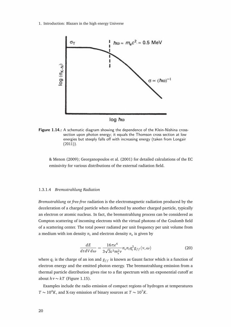
1. Introduction: Blazars in the high energy Universe
Figure 1.14.: A schematic diagram showing the dependence of the Klein-Nishina cross-section upon photon energy; it equals the Thomson cross section at lowenergies but steeply falls off with increasing energy (taken from Longair(2011)).
& Menon (2009); Georganopoulos et al. (2001) for detailed calculations of the EC
emissivity for various distributions of the external radiation field.
1.3.1.4 Bremsstrahlung Radiation
Bremsstrahlung or free-free radiation is the electromagnetic radiation produced by the
deceleration of a charged particle when deflected by another charged particle, typically
an electron or atomic nucleus. In fact, the bremsstrahlung process can be considered as
Compton scattering of incoming electrons with the virtual photons of the Coulomb field
of a scattering center. The total power radiated per unit frequency per unit volume from
a medium with ion density ni and electron density ne is given by
dEd tdV dω
=16πe4
3p
3c3m2e v
neniq2i g f f (v,ω) (20)
where qi is the charge of an ion and g f f is known as Gaunt factor which is a function of
electron energy and the emitted photon energy. The bremsstrahlung emission from a
thermal particle distribution gives rise to a flat spectrum with an exponential cutoff at
about hν∼ kT (Figure 1.15).
Examples include the radio emission of compact regions of hydrogen at temperatures
T ∼ 104K , and X-ray emission of binary sources at T ∼ 107K .
20

1.3. Radiative mechanisms
Figure 1.15.: Intensity spectrum (arbitrary units) of bremsstrahlung radiation due to athermal electron distribution at temperature 100 keV. Note the exponen-tial cutoff at high energies. Figure reproduced from Sunder Sahayanathan(2011).
1.3.2 Hadronic Processes
If protons are accelerated to sufficiently high energies, hadronic interactions and syn-
chrotron emission start to play a significant role. The characteristic frequency of the
emitted synchrotron radiation by a proton of energy γpc2 is (mp/me)3 ∼ 6×10⁹ times
smaller than the characteristic frequency of synchrotron photons emitted by an electron
of the same energy. The hadronic models have been discussed extensively by several
authors, (see, for eg: Aharonian (2004) and Kelner et al. (2006) for discussions and
references). Here, we briefly list the most dominant processes.
1.3.2.1 Bethe-Heitler Process
A gamma ray photon (γ) can interact with a nucleon N to give rise to an electron positron
pair according to the equation,
N + γ→ N + e++ e− (21)
These electron-positron pairs can undergo cascading giving rise to a hadronically induced
secondary synchrotron and IC emission components. The threshold energy for this
process in the nucleon rest frame is the sum of the rest mass energies of the electron and
positron, 1.022 MeV.
21
1. Introduction: Blazars in the high energy Universe
1.3.2.2 Pion and meson decays
Inelastic p-p interactions of high energy protons and other nuclei with the ambient matter
produce pions and mesons whose subsequent decay gives rise to high energy gamma
rays via the following channels,
η→ 2γ (22)
η→ 3π0 (23)
π0→ 2γ (24)
π+(π−)→ µ+(µ−)+νµ(νµ) (25)
µ+(µ−)→ e+(e−)+νe(νe) (26)
Protons also interact with high energy gamma rays (above the threshold energy of
145 MeV) to produce neutral and charged pions, which further decay as shown above.
1.4 B L A Z A R S E M I S S I O N M O D E L S
The inferred high luminosities, apparent superluminal velocities and observed rapid
variabilities provide us with reasonable evidence that the broadband non-thermal contin-
uum from blazar jets is produced from a small (R< 1 day) emission region propagating
relativistically at a small angle to our line of sight. While the origin of the low-energy
component of the SED is well established to be caused by synchrotron emission from
relativistic electrons gyrating in the magnetic field of the jet, the physical mechanisms
responsible for the high-energy emission are still under debate. If the protons are not
accelerated to sufficiently high energies to reach the threshold for pγ pion production,
the high-energy radiation will be dominated by IC emission from the ultra-relativistic
electrons in the jet (leptonic models). In the opposite case, the high-energy emission
will be dominated by proton, pion and muon synchrotron and/or cascades initiated from
proton-proton interactions (hadronic models). A comprehensive review of these mecha-
nisms may be found in Boettcher (2010). However, with current spectral information, it
is difficult to rule out any of these models (Figure 1.16).
1.4.1 Leptonic models
In leptonic models, the high-energy emission is produced via IC scattering of soft photons
by the same ultra-relativistic electrons which are producing the synchrotron emission.
The seed photons for the up-scattering may be the synchrotron photons themselves
(SSC; eg: Marscher & Gear (1985); Maraschi et al. (1992); Böttcher et al. (2009)) or
22

1.4. Blazars emission models
the ambient photons outside the jet (EC). The sources of EC photons, which play an
important role in our understanding of the AGN environments, include:
• Photons from the accretion disk (Dermer et al., 1992; Dermer & Schlickeiser, 1993)
• Reprocessed optical-UV emission from the BLR (Sikora et al., 1994; Blandford &
Levinson, 1995; Ghisellini & Madau, 1996; Dermer et al., 1997)
• IR photons from the dusty torus (Błazejowski et al., 2000)
In its simplest case, emission is assumed to come from a single emission zone of speci-
fied geometrical shape, mostly spherical, with an adhoc specified electron distribution.
A more realistic approach consists of self-consistent steady-state solution of the Fokker-
Planck equation including a physically motivated (e.g., from shock-acceleration theory)
acceleration of particles and all relevant radiative and adiabatic cooling mechanisms
(Weidinger et al., 2010; Acciari et al., 2009c; Ghisellini & Tavecchio, 2009). Time depen-
dent SSC/SSC+EC models have been developed which incorporate electron dynamics
and radiation transfer factors to reproduce the observed variabilities (Li & Kusunose,
2000; Kataoka et al., 2000; Sikora et al., 2001; Böttcher & Chiang, 2002). Hadrons are
assumed to be cold, and are involved only in the propagating the kinetic energy of the
jet.
While leptonic models are highly successful in reproducing the blazar SEDs and
lightcurves in most cases, specially the correlated X-ray/TeV variability usually seen
in most HBLs (Coppi & Aharonian, 1999), some recent observations pose a serious
challenge. Detection of minute scale flux doubling time scales (Paliya et al., 2015a;
Aharonian et al., 2007c) requires a size of the emitting region that might be smaller than
the Schwarzschild radius of the central black hole of the AGN (Begelman et al., 2008).
Intrinsic TeV spectra of distant blazars have been found to require very “hard" particle
indices (< 1.5), which is not possible to accommodate within known acceleration theory
models Aharonian et al. (2006b). Observations of “orphan" flares at TeV energies are
also puzzling.
1.4.1.1 Inhomogeneous jet models
To address some of the failures of the simple one zone models, phenomenological multi-
zone models have been introduced by several authors. Tavecchio & Ghisellini (2008), in
order to explain the minute scale VHE flares from PKS 2155+304, proposed a spine-sheath
model where the γ-ray emission originates from a small spine of ultra-relativistic plasma
within a larger, slower moving jet. Georganopoulos & Kazanas (2003) used a decelerating-
jet model where differential relativistic motion between various emission zones leads to
Doppler boosting of one zone’s emission into the rest frame of another zone. This can
reduce the requirements of extreme bulk Lorentz (and Doppler) factors inferred from
simple one-zone letponic modeling, and reproduce SEDs with more “reasonable" sets of
23
1. Introduction: Blazars in the high energy Universe
parameters. Even further improvements upon these models have been carried out in the
shock-in-jet models (Böttcher & Dermer, 2002; Joshi, 2009; Mimica et al., 2004; Sokolov
& Marscher, 2005), where the time dependent evaluation of retarded radiation fields
originating from all parts of the shocked regions of the jet are considered.
1.4.2 Hadronic models
As an alternate to leptonic models, hadronic models have been proposed where a signifi-
cant fraction of the jet power is converted into the acceleration of relativistic protons
in a strongly magnetized environment. The acceleration of protons to the necessary
ultra-relativistic energies (Ep > 1019 eV) requires high magnetic fields of several tens
of Gauss. In the presence of such high magnetic fields, the synchrotron radiation of the
primary protons, and secondary muons and pions, also need to be accounted for (Rachen
& Mészáros, 1998; Mücke et al., 2000; Mücke & Protheroe, 2001). Electromagnetic
cascades are then generated as discussed in Section 1.3.2 (Mannheim & Biermann, 1989,
1992).
Hadronic models are difficult to investigate in a time-dependant way due to the
required computer intensive Monte Carlo simulations. However, observations of rapid
time variabilities seem inconsistent with the radiative cooling time scales of protons.
Correlated X-ray/TeV flares are also difficult to explain within the ambit of hadronic
models. On the other hand, “orphan" flares and “hard" TeV spectra can be naturally
explained.
1.5 O P E N Q U E S T I O N S A B O U T A G N J E T S
Despite the considerable volume of work available in this field, the physics of the ubiqui-
tous astrophysical jets remain heavily shrouded in debate. The jet formation, collimation
and acceleration are still only vaguely understood. The observed rapid variability suggests
that the emission region is compact and located close to the nucleus (Dondi & Ghisellini,
1995), which lies below the resolution limit of modern facilities. Thus, even the sites
of production of radiation at different energies are also not well known. AGN activity
is triggered by galaxy mergers/interactions. As such, AGN activity is directly linked to
the structure formation in the Universe. Also, outflows, jets, and high-energy radiation
produced in AGN may substantially influence the surrounding (galactic and intergalactic)
medium, modifying therefore the structure formation itself via some complex feedback
process. Studying how AGN evolve with redshift is therefore important for understanding
cosmological evolution of galaxies in general. In this section, we list some of the most
exciting unsolved questions in this field, which we hope can be resolved in the upcoming
years.
24

1.5. Open questions about AGN jets
Figure 1.16.: Fits to the SED of 3C279, reproduced from Boettcher (2010). The heavysolid curve is an attempt of a leptonic model with EC dominated γ-ray emis-sion, while the dotted curve is a SSC fit to the X-ray through γ-ray spec-trum. The dashed and dot-dashed curves are hadronic model fits.
1.5.1 Jet formation
Theoretical models for the production of relativistic jets from active galactic nuclei predict
that jet power arises from the spin and mass of the central supermassive black hole, as
well as from the magnetic field near the event horizon (Blandford & Znajek, 1977). The
physical mechanism underlying the contribution from the magnetic field is the torque
exerted on the rotating black hole by the field amplified by the accreting material. It
has been shown by Ghisellini et al. (2014) that while there is a clear linear relationship
between the accretion disk luminosity and the gamma ray power of their jets, the jet
luminosity outshines that of the disk by more than an order of magnitude, implying that
disks alone cannot power the jets; the black hole’s spin must also be involved. However, it
may also be possible that the magnetic field extracts power out of the accretion disk, thus
making it appear less bright. Difficulties in measuring the blackhole spin presently pose
problems in our understanding of the jet launching mechanisms, and present observations
are far from resolving the launch region for any blackhole.
1.5.2 Jet propagation and acceleration
How and why jets remain collimated over such large distances (∼ 100 kpc) is an unsolved
question. Calculations of the jet power are subject to various uncertainties, like the
amount of e+e− pairs and the contribution of hot protons. Are jets matter or Poynting
25
1. Introduction: Blazars in the high energy Universe
flux dominated? To the best of knowledge, particles are accelerated at relativistic shocks
inside the jets, but an absence of observational proof prevents us from establishing
this fact. Here, polarization mapping might give us more hints on the constraining
magnetic field, and clearly higher-resolution, higher-cadence radio observations along
with higher fidelity numerical modeling are our pathway towards understanding jet
structures (Beckmann & Shrader, 2012a).
1.5.3 Questions specific to blazars
While the unified AGN model is reasonably accepted by the scientific community, it needs
to be subjected to stringent observational results. We do not well understand why some
AGNs are radio-loud and some radio-quiet. Though Fermi has much revolutionised our
understanding of the γ-ray emission from blazars, the location and structure of γ-ray
emitting regions in AGN jets are not well known. The origin of seed photons for IC
scattering are not well clear. It needs to be understood if there are multiple emission
zones, or a single one, as well as the underlying electron energy spectra and the particle
acceleration processes involved. Since high quality SEDs are obtained only during flaring
state, we have a very poor understanding of the average emission state of blazars. Thus,
why and how blazars flare remain largely unknown. The observed variability patterns
over all timescales are yet to receive a proper theoretical treatment. The hard TeV spectra
seen in distant blazars after deconvolution with theoretical EBL models (see Chapter
7 ) are a challenge for current acceleration theories. Alternatively they may indicate a
problem with our understanding of cosmological EBL models.
1.6 A I M O F T H I S T H E S I S
The aim of this thesis is to investigate the energy content of the jets, specifically looking
at the validity of the leptonic models. By concentrating on the multi-wavelength spectral
and temporal variability of two TeV blazars, we try to understand the underlying particle
spectra and the means to achieve the same. A study of the long term flux distribution and
variability also gives us interesting new clues into the probable jet launching mechanisms.
We also obtain a model independent estimate of the EBL from a statistical study of all
detected TeV blazars.
• Chapter 1 provides a brief introduction into the exciting world of blazar physics,
with emphasis on the high energy radiation and detection mechanisms at the
highest energies.
• Chapter 2 describes the instrumentation, data reduction and analysis methods for
the HAGAR Telescope Array, an ACT array at Hanle, Ladakh.
26

1.6. Aim of this thesis
• Chapter 3 details the sources of multi-wavelength data and associated data reduc-
tion algorithms.
• Chapter 4 describes our long term study of Mkn 421 from 2009-2015, and results
from the same.
• Chapter 5 focusses specially on the huge and rapid X-ray flare seen from the
aforementioned source in April 2013.
• Chapter 6 reports on a multi-epoch multi-frequency spectral study of 1ES 1011+496
to understand a plausible origin for a curved particle distribution.
• Chapter 7 elucidates a novel method of estimating the EBL from a statistical study
of TeV blazars.
• Chapter 8 concludes with our findings and some prospects for the future.
27

"Equipped with his five senses, man explores the universe
around him and calls the adventure Science."
Edwin Hubble
2The HAGAR Telescope Array
THE HIGH ALTITUDE GAMMA RAY (HAGAR) TELESCOPE ARRAY (Figure 2.1) is a hexagonal
array of ACTs which uses the wavefront sampling technique to detect celestial gamma
rays. It is located at the Indian Astronomical Observatory site (32 46’ 46" N, 78 58’ 35"
E), in Hanle, Ladakh in the Himalayan mountain ranges at an altitude of 4270 m above
mean sea level. Since the Cherenkov photon density of a shower increases with altitude,
a low energy threshold is achieved by operating at such high altitudes. Proposal for
HAGAR experiment was made in 2001, and the first telescope installed in 2005. Regular
science runs are being conducted since September 2008.
In this chapter, we discuss the design and instrumentation of the HAGAR telescope,
the simulations carried out to understand the performance parameters, the observation
methods, and the data reduction and analysis techniques.
2.1 T H E T E L E S C O P E A R R AY: D E S I G N A N D I N S T R U M E N TAT I O N
The HAGAR Telescope Array (Chitnis et al., 2011) consists of seven telescopes, with six
telescopes located at the vertices of a hexagon and one at the center. The separation
between two nearest telescopes is 50m, and opening angle (Field of View) of the HAGAR
telescopes is 3. The total reflector area per telescope is ∼ 4.45 m2 with the average
mirror reflectivity at ∼ 80%. Figure 2.2 shows a schematic layout of the HAGAR array.
Each of the seven telescopes has seven para-axially mounted front coated parabolic
mirrors of diameter 0.9 m (and f /d ∼ 1), with a fast, high gain UV-sensitive Photonis
photo-multiplier tube (PMT), XP2268B, at the focus of individual mirrors. These PMTs
have good sensitivity to photons in the ultraviolet to blue range, with a peak quantum
29

2. The HAGAR Telescope Array
Figure 2.1.: The HAGAR Telescope Array located at Hanle, Ladakh. (Photo Credits: AjayTalwar)
Figure 2.2.: Schematic layout of the the HAGAR Array. The hexagonal array has a radiusof 50m, and each telescope has 7 PMTs in a hexagonal array.
30

2.2. Data Acquisition system (DAQ)
efficiency of about 24 % at 400 nm. At typical operating voltages (∼ 1700 − 1800 V),
the rate of afterpulses was found to be negligible (∼ 1−2%).
Each of the seven telescopes uses an alt-azimuthal mounting, with each axis of the
telescope driven by a stepper motor. The telescope movement control system consists of
two 17-bit Rotary encoders, two stepper motors and a micro-controller based Motion
Control Interface Unit (MCIU). Steady state pointing accuracy of the servo is ±10 arc-
sec with maximum slew rate of 30 deg/minute. The resulting blind spot size while
tracking the stars near zenith is found to be less than 0.6 deg. The telescope movement
is manoeuvred by a control software written on a Linux platform. The pointing of
the telescopes is continuously monitored and corrected in real time during tracking.
A detailed pointing model was developed Gothe et al. (2013) to attain good pointing
accuracy of mean direction of 7 mirrors in each telescope as well as low spread in pointing
directions of mirrors about this mean.
To check the pointing accuracy of each mirror, regular bright star scans (BS Scans),
are carried out where the telescope is aligned to an isolated bright star (around V-band
magnitude ∼ 2−2.5), then moved to the West by 5, and the telescope tracking switched
off. The counting rates of each PMT are monitored. The star is allowed to drift into the
field of view of the mirrors and out of it. The PMT count rates corresponding to each
mirror are then used to find the pointing offset. However, this method can be used to
measure the offset only in the East-West direction.
A better method is to use the RA-Dec scans, which can give the pointing offsets along
both axis. At the beginning of the RA scan, the telescope control program acquires
and tracks the bright star. Then, a series of manual offsets in the stars RA coordinates
are introduced while holding onto the star’s declination (i.e. declination offset = 0),
and the PMT monitoring rates recorded. Similarly, for a Dec scan, a series of manual
offsets in declination coordinates are introduced while holding onto the RA coordinate
of the star (i.e. RA offset = 0) and the PMT pulse rates recorded. The PMT count
rate is plotted as a function of the offset angle, and the central value of the profile
gives the offset between the telescope and the mirror pointing direction. This offset is
manually corrected by mechanical re-alignment of the mirrors, and the scan repeated till
satisfactory profile obtained. Figure 2.3 shows a typical profile obtained during a bright
star scan. The overall pointing accuracy of HAGAR telescope mirrors achieved by this
method is 0.23±0.10, as shown in Fig 2.4.
2.2 DATA A C Q U I S I T I O N S Y S T E M (DA Q)
HAGAR operates on a interrupt driven CAMAC based DAQ. The PMT high voltages of ∼1700 V, controlled using a C.A.E.N. controller model SY1527, are adjusted for a PMT rate
of 5 kHz. This equality of the PMT rates ensures equal efficiency for each channel. The
seven PMT pulses of a telescope are amplified 10 times using an amplifier module, and
31

2. The HAGAR Telescope Array
(a) Mis-aligned mirror (b) Aligned mirror
Figure 2.3.: PMT count rates from a Bright Star scan conducted in May 2013, for a typi-cal misaligned and well aligned mirror, respectively.
Pointing on the sky...All mirrors..(September2015)
N Radius
1.0
0.75
0.50
0.25
degree
E
0.10 deg±Pointing error: 0.23
Symbol(Az,Zd)
(95.41,22.36)
(223.45,12.83)
(93.85,24.34)
Tel#1
Tel#2
Tel#3
Tel#4
Tel#5
Tel#6
Tel#7
Figure 2.4.: Pointing offset for HAGAR mirrors after alignment for three separate starscans in September 2015.
32
2.3. Observations
then linearly added to form a telescope output called the Royal Sum (RS) pulse, which is
brought to the control room (situated below the central telescope) via low attenuation
coaxial cables of types LMR-ultraflex-400 and RG 213 with total length of about 85m.
The corresponding information of the RS pulses from each telescope are recorded. Data
recorded for each event consist of relative arrival times of Cherenkov shower front at
each mirror, as measured by Time to Digital Converters (TDC) with a resolution of 0.25
ns. A real time clock (RTC) module synchronized with GPS is used to record the absolute
arrival time of these events, accurate up to µs. The pulse height information of the
showers is measured using 12 bit Charge to Digital Converters (QDC). Information of the
triggered telescopes and other house-keeping information are also recorded. The PMT
count rates are monitored using at regular intervals using a monitor interrupt arriving at
1 Hz frequency.
An event trigger is generated on coincidence of at least 4 out of 7 telescope pulses in
narrow coincidence window of 60 ns, above a pre-assigned discriminator threshold of
around 200 mV. This corresponds the condition Number of Triggered Telescopes (NTT)
¾ 4. Plot of observed trigger rate vs discriminator threshold is shown in Figure 2.5. The
discriminator biases are adjusted to keep the RS rates within 25-35 kHz to maintain a
chance coincidence rate within a few percent of the trigger rate. The diagrams showing
all the modules of the telescope electronics and trigger distribution in DAQ are shown in
Figure 2.6 and Figure 2.7, respectively. The TDC start pulses are generated on an event
trigger. Since there is finite delay required to form the trigger, the RS pulses are delayed
using ECL-based digital delays before they are fed into individual TDC stops. A Common
QDC gate is also generated on event trigger. Analog RS pulses from a Fan-in/Fan-out
module are delayed using cables and taken to Phillips QDC module.
In addition to the main DAQ system, a parallel DAQ ( 4 channel modules of ACQIRIS
make model DC271A) using commercial 8 bit waveform digitizers with 1 GHz bandwidth
with 50 ohm resistance and a sampling rate of 1 GS/s is also being used. The seven RS
pulses from the seven telescopes are input to this module. This is enabling us to study
the pulse shape, and use the same to reduce the NSB contribution by restricting the time
window around the Cherenkov pulse.
2.3 O B S E RVAT I O N S
Observations with the HAGAR telescope array are carried out during clear moonless
night, roughly 7-10 days centered around each new moon. Since the commencement of
regular science observations in September 2008, a total of 4740 hrs of observation have
been carried out (till March, 2016). Observations are generally carried out for more the
70 % of the total available time. Different types of observations (Figure 2.8) are carried
out each season, the details of which are outlined below:-
1. ON-source run
33

2. The HAGAR Telescope Array
Figure 2.5.: Plot of observed trigger rate as a function of the discriminator bias voltagefor four fold trigger rate. The chance rate dominates over the shower gener-ated trigger rate at low voltages, but becomes negligible at high voltages.
Figure 2.6.: Flowchart of telescope electronics in the HAGAR DAQ.
34
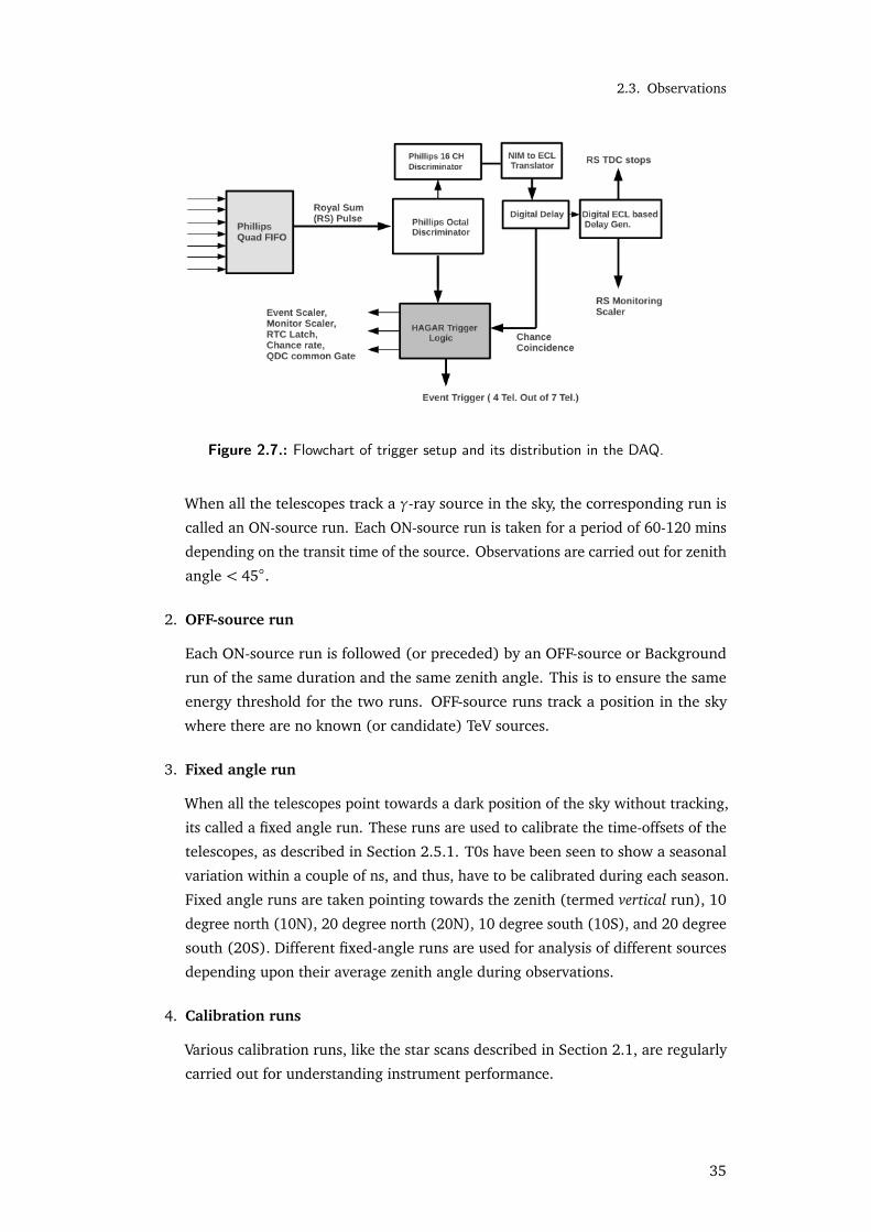
2.3. Observations
Figure 2.7.: Flowchart of trigger setup and its distribution in the DAQ.
When all the telescopes track a γ-ray source in the sky, the corresponding run is
called an ON-source run. Each ON-source run is taken for a period of 60-120 mins
depending on the transit time of the source. Observations are carried out for zenith
angle < 45.
2. OFF-source run
Each ON-source run is followed (or preceded) by an OFF-source or Background
run of the same duration and the same zenith angle. This is to ensure the same
energy threshold for the two runs. OFF-source runs track a position in the sky
where there are no known (or candidate) TeV sources.
3. Fixed angle run
When all the telescopes point towards a dark position of the sky without tracking,
its called a fixed angle run. These runs are used to calibrate the time-offsets of the
telescopes, as described in Section 2.5.1. T0s have been seen to show a seasonal
variation within a couple of ns, and thus, have to be calibrated during each season.
Fixed angle runs are taken pointing towards the zenith (termed vertical run), 10
degree north (10N), 20 degree north (20N), 10 degree south (10S), and 20 degree
south (20S). Different fixed-angle runs are used for analysis of different sources
depending upon their average zenith angle during observations.
4. Calibration runs
Various calibration runs, like the star scans described in Section 2.1, are regularly
carried out for understanding instrument performance.
35

2. The HAGAR Telescope Array
Figure 2.8.: Bar chart showing the amount of HAGAR observation time spent of differentobservation types. ON and OFF source runs are conducted for both galacticand extragalactic sources. Calibration runs include fixed angle runs, brightstar scans, etc.
2.4 S I M U L AT I O N S
Simulations play a crucial role in the HAGAR experiment. Since we cannot produce VHE
gamma rays in the laboratory, direct calibration of the telescope is impossible. Rather,
the HAGAR performance parameters, like for all other ACTs, are understood through
detailed Monte Carlo simulations (Saha et al., 2013). Simulations for HAGAR have two
principal components:
1. Showers simulations: Extensive Air Showers propagating in the atmosphere are
simulated using the CORSIKA simulation package (v. 2.720) developed by the
KASCADE group Heck et al. (1998). Spectral index of the primary γ-rays is used in
accordance to the measured Crab nebulae spectrum Aharonian et al. (2000), which
is the standard candle for all VHE experiments. Electron, proton, alpha particle
showers are simulated according to the measured cosmic ray spectrum between the
energy ranges 20 GeV to 5 TeV, 50 GeV to 5 TeV and 100 GeV to 10 TeV, respectively.
The VENUS code is used for high energy hadronic interactions, GHEISHA for low
energy ones. For electromagnetic interactions, the EGS4 code is used. Showers
are simulated for various inclination angles from 0 to 45. Due to the absence of
atmospheric profile measurements at Hanle, US standard atmospheric profile is
used.
36
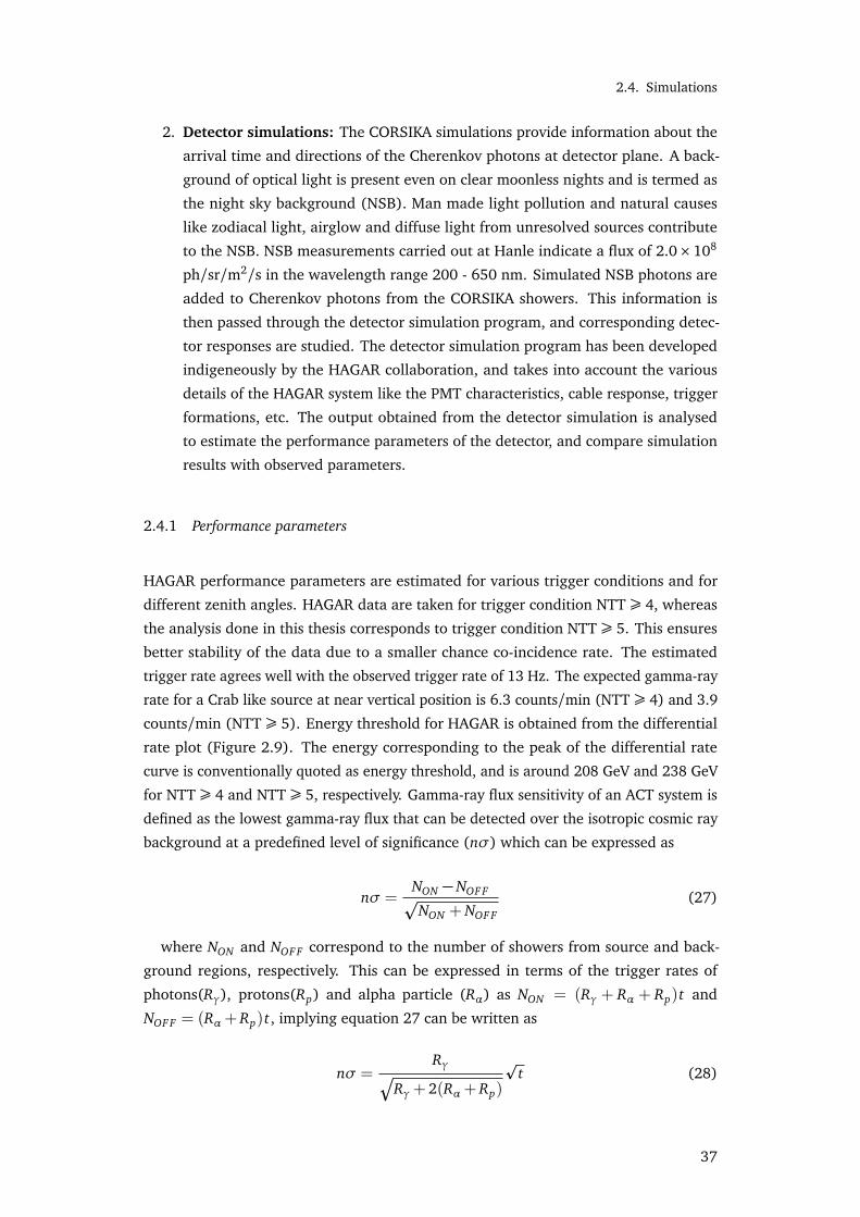
2.4. Simulations
2. Detector simulations: The CORSIKA simulations provide information about the
arrival time and directions of the Cherenkov photons at detector plane. A back-
ground of optical light is present even on clear moonless nights and is termed as
the night sky background (NSB). Man made light pollution and natural causes
like zodiacal light, airglow and diffuse light from unresolved sources contribute
to the NSB. NSB measurements carried out at Hanle indicate a flux of 2.0×10⁸
ph/sr/m2/s in the wavelength range 200 - 650 nm. Simulated NSB photons are
added to Cherenkov photons from the CORSIKA showers. This information is
then passed through the detector simulation program, and corresponding detec-
tor responses are studied. The detector simulation program has been developed
indigeneously by the HAGAR collaboration, and takes into account the various
details of the HAGAR system like the PMT characteristics, cable response, trigger
formations, etc. The output obtained from the detector simulation is analysed
to estimate the performance parameters of the detector, and compare simulation
results with observed parameters.
2.4.1 Performance parameters
HAGAR performance parameters are estimated for various trigger conditions and for
different zenith angles. HAGAR data are taken for trigger condition NTT ¾ 4, whereas
the analysis done in this thesis corresponds to trigger condition NTT ¾ 5. This ensures
better stability of the data due to a smaller chance co-incidence rate. The estimated
trigger rate agrees well with the observed trigger rate of 13 Hz. The expected gamma-ray
rate for a Crab like source at near vertical position is 6.3 counts/min (NTT ¾ 4) and 3.9
counts/min (NTT ¾ 5). Energy threshold for HAGAR is obtained from the differential
rate plot (Figure 2.9). The energy corresponding to the peak of the differential rate
curve is conventionally quoted as energy threshold, and is around 208 GeV and 238 GeV
for NTT ¾ 4 and NTT ¾ 5, respectively. Gamma-ray flux sensitivity of an ACT system is
defined as the lowest gamma-ray flux that can be detected over the isotropic cosmic ray
background at a predefined level of significance (nσ) which can be expressed as
nσ =NON −NOF Fp
NON +NOF F(27)
where NON and NOF F correspond to the number of showers from source and back-
ground regions, respectively. This can be expressed in terms of the trigger rates of
photons(Rγ), protons(Rp) and alpha particle (Rα) as NON = (Rγ + Rα + Rp)t and
NOF F = (Rα+Rp)t, implying equation 27 can be written as
nσ =Rγ
q
Rγ+ 2(Rα+Rp)
pt (28)
37

2. The HAGAR Telescope Array
Figure 2.9.: Differential rate plots for different zenith angles for the ¾ 4 (red), ¾ 5(brown), ¾ 6 (blue) and = 7 (green) trigger conditions; taken from Sahaet al. (2013).
Thus, the integration time required to obtain a significant detection depends on the
flux level of the source. Figure 2.10 hows the observation duration needed for HAGAR
to detect a source at 5σ significance level as a function of the source flux in units of
the Crab flux, implying that HAGAR will be able to detect a Crab Nebula like source
at a significance level of 5σ in 17 hours of observation duration. This sensitivity could
be further improved if more cosmic ray background events are rejected by imposing
additional criteria.
2.5 DATA R E D U C T I O N A N D A N A LY S I S
Data reduction technique for HAGAR telescope is derived from the method used for
the data analysis of PACT experiment at Pachmarhi (Bose et al., 2007). Analysis codes
are developed in-house in IDL language with Python wrapper routines. Source flux is
computed by comparing the number of cosmic shower events from the source region
with similar background region.
2.5.1 Space Angle Estimation
The difference between the reconstructed arrival direction and the telescope pointing
direction (space angle) is computed in two steps, by first correcting for fixed time offsets
in the system (T0) and then the estimation of the direction of air shower is done by
measuring the relative arrival time of Cherenkov wavefront induced by the shower at
each telescope. The details of the steps are outlined below:-
1. Computation of T0:
38
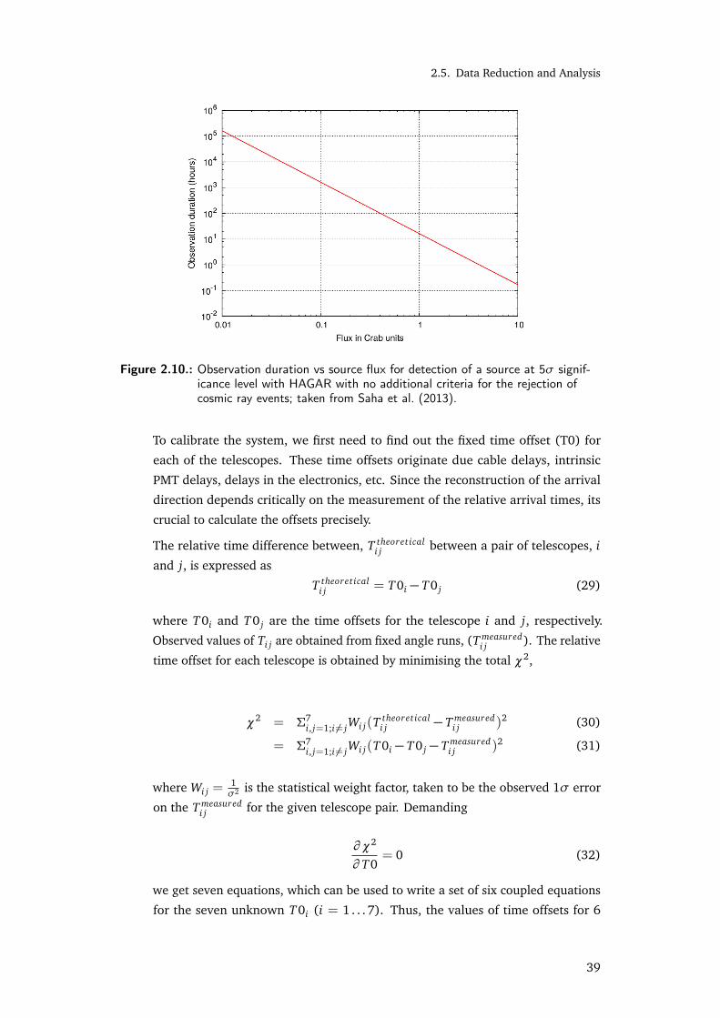
2.5. Data Reduction and Analysis
Figure 2.10.: Observation duration vs source flux for detection of a source at 5σ signif-icance level with HAGAR with no additional criteria for the rejection ofcosmic ray events; taken from Saha et al. (2013).
To calibrate the system, we first need to find out the fixed time offset (T0) for
each of the telescopes. These time offsets originate due cable delays, intrinsic
PMT delays, delays in the electronics, etc. Since the reconstruction of the arrival
direction depends critically on the measurement of the relative arrival times, its
crucial to calculate the offsets precisely.
The relative time difference between, T theoret icali j between a pair of telescopes, i
and j, is expressed as
T theoret icali j = T0i − T0 j (29)
where T0i and T0 j are the time offsets for the telescope i and j, respectively.
Observed values of Ti j are obtained from fixed angle runs, (T measuredi j ). The relative
time offset for each telescope is obtained by minimising the total χ2,
χ2 = Σ7i, j=1;i 6= jWi j(T theoret ical
i j − T measuredi j )2 (30)
= Σ7i, j=1;i 6= jWi j(T0i − T0 j − T measured
i j )2 (31)
where Wi j =1σ2 is the statistical weight factor, taken to be the observed 1σ error
on the T measuredi j for the given telescope pair. Demanding
∂ χ2
∂ T0= 0 (32)
we get seven equations, which can be used to write a set of six coupled equations
for the seven unknown T0i (i = 1 . . . 7). Thus, the values of time offsets for 6
39
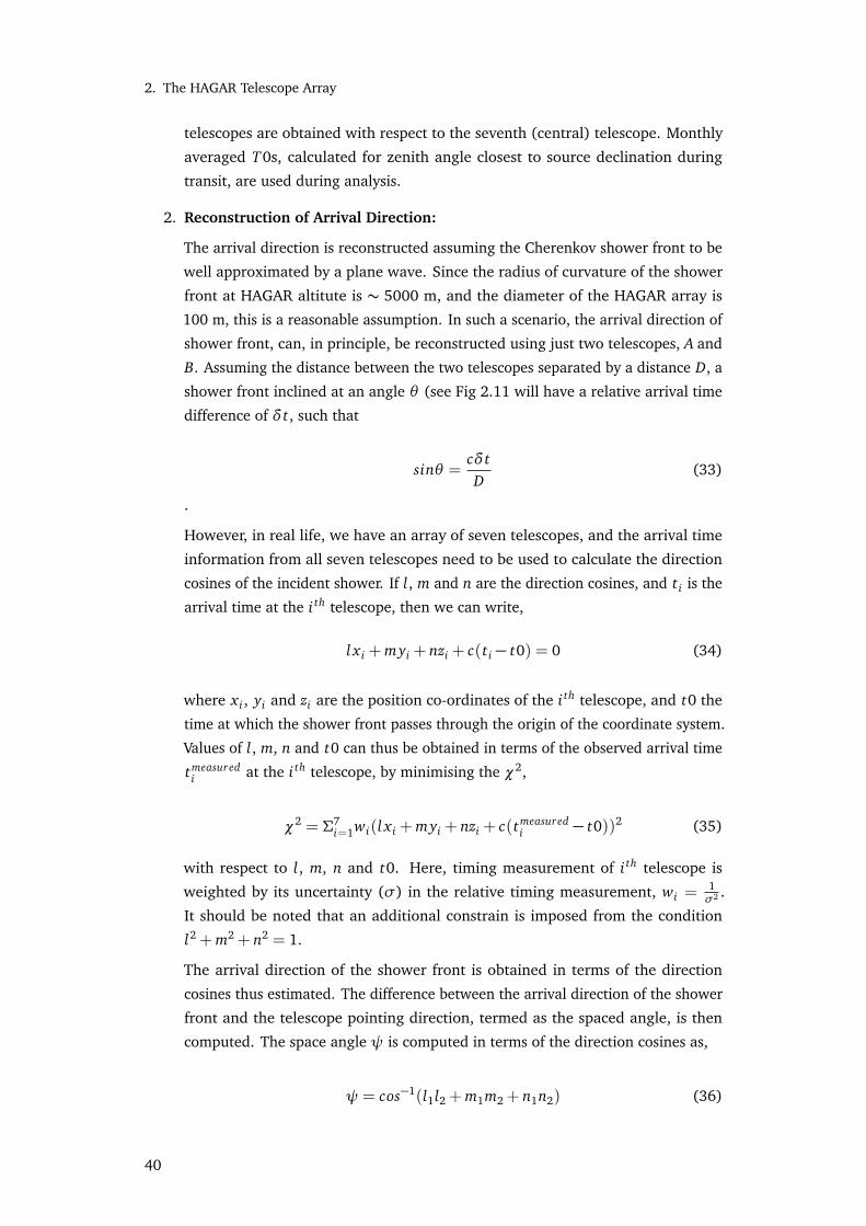
2. The HAGAR Telescope Array
telescopes are obtained with respect to the seventh (central) telescope. Monthly
averaged T0s, calculated for zenith angle closest to source declination during
transit, are used during analysis.
2. Reconstruction of Arrival Direction:
The arrival direction is reconstructed assuming the Cherenkov shower front to be
well approximated by a plane wave. Since the radius of curvature of the shower
front at HAGAR altitute is ∼ 5000 m, and the diameter of the HAGAR array is
100 m, this is a reasonable assumption. In such a scenario, the arrival direction of
shower front, can, in principle, be reconstructed using just two telescopes, A and
B. Assuming the distance between the two telescopes separated by a distance D, a
shower front inclined at an angle θ (see Fig 2.11 will have a relative arrival time
difference of δt, such that
sinθ =cδtD
(33)
.
However, in real life, we have an array of seven telescopes, and the arrival time
information from all seven telescopes need to be used to calculate the direction
cosines of the incident shower. If l, m and n are the direction cosines, and t i is the
arrival time at the i th telescope, then we can write,
l x i +myi + nzi + c(t i − t0) = 0 (34)
where x i, yi and zi are the position co-ordinates of the i th telescope, and t0 the
time at which the shower front passes through the origin of the coordinate system.
Values of l, m, n and t0 can thus be obtained in terms of the observed arrival time
tmeasuredi at the i th telescope, by minimising the χ2,
χ2 = Σ7i=1wi(l x i +myi + nzi + c(tmeasured
i − t0))2 (35)
with respect to l, m, n and t0. Here, timing measurement of i th telescope is
weighted by its uncertainty (σ) in the relative timing measurement, wi =1σ2 .
It should be noted that an additional constrain is imposed from the condition
l2 +m2 + n2 = 1.
The arrival direction of the shower front is obtained in terms of the direction
cosines thus estimated. The difference between the arrival direction of the shower
front and the telescope pointing direction, termed as the spaced angle, is then
computed. The space angle ψ is computed in terms of the direction cosines as,
ψ= cos−1(l1l2 +m1m2 + n1n2) (36)
40
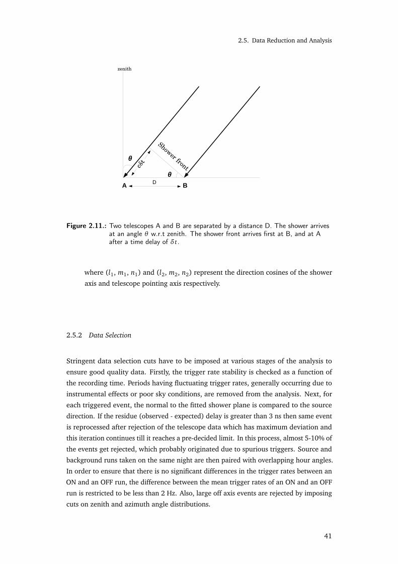
2.5. Data Reduction and Analysis
θ
θ
Shower front
A BD
ctδ
zenith
Figure 2.11.: Two telescopes A and B are separated by a distance D. The shower arrivesat an angle θ w.r.t zenith. The shower front arrives first at B, and at Aafter a time delay of δt.
where (l1, m1, n1) and (l2, m2, n2) represent the direction cosines of the shower
axis and telescope pointing axis respectively.
2.5.2 Data Selection
Stringent data selection cuts have to be imposed at various stages of the analysis to
ensure good quality data. Firstly, the trigger rate stability is checked as a function of
the recording time. Periods having fluctuating trigger rates, generally occurring due to
instrumental effects or poor sky conditions, are removed from the analysis. Next, for
each triggered event, the normal to the fitted shower plane is compared to the source
direction. If the residue (observed - expected) delay is greater than 3 ns then same event
is reprocessed after rejection of the telescope data which has maximum deviation and
this iteration continues till it reaches a pre-decided limit. In this process, almost 5-10% of
the events get rejected, which probably originated due to spurious triggers. Source and
background runs taken on the same night are then paired with overlapping hour angles.
In order to ensure that there is no significant differences in the trigger rates between an
ON and an OFF run, the difference between the mean trigger rates of an ON and an OFF
run is restricted to be less than 2 Hz. Also, large off axis events are rejected by imposing
cuts on zenith and azimuth angle distributions.
41
2. The HAGAR Telescope Array
2.5.3 Signal Extraction
Gamma-ray events are separated from the isotropic background of cosmic rays by com-
paring the space angle distributions of ON-source runs and OFF-source runs. By choice
of OFF region, OFF-source runs are devoid of γ-ray events, and contain only cosmic
ray events, whereas, ON-source runs contain both γ and cosmic ray events. However,
a simple subtraction of the number of OFF-source events (NOF F ) from the number of
ON-source events (NON ) cannot be used to obtain the source signal. Since the ON-source
runs and OFF-source runs are taken at two different times in the same night, the sky
conditions may be different for two different runs and we need to normalize NOF F w.r.t.
NON .
The space angle distributions are compared for ON and OFF souce events. γ-ray
events from the source are expected to come only within the narrow Cherenkov cone
large space angle events are should be only cosmic-ray triggered events, in both ON and
OFF runs. Figure 2.12 shows the space angle distributions for a typical ON and OFF
source runs. The region beyond the FWHM of the ON-source distribution is taken as the
lower normalisation region (LNR), and the common end point as upper normalization
region (UNR). Number of events in the normalization region are typically around 15-20%,
depending upon the sky brightness and operating conditions. The normalisation constant,
C , is computed as
C =ΣUNR
LNR NON
ΣUNRLNR NOF F
(37)
Excess/deficit signal (S) is then calculated from events which lie between the telescope
axis (0-degree) and LNR, given by
S = ΣLNR0 (NON − CNOF F ) (38)
The normalization constant is estimated for each selected ON-OFF pair and then the
excess/deficit signal is calculated. The LNR and UNR cuts have been optimised to get
null signal for analysis of dark runs. Only run pairs having C within the range 0.8−1.2
are retained during analysis.
2.6 R E S U LT S
Routine observations of AGNs, pulsars and supernova remnants are being carried out
with HAGAR. While for the first two years observations could not be carried out for
about three months during winter due to lack of manpower at site, observations are
being taken throughout the year since 2010. Almost 38% of the observation time has
been spent on galactic sources, with majority of the time spent on the Crab Nebula
for calibration purposes, and also to search for pulsations. VHE photons of energies
42
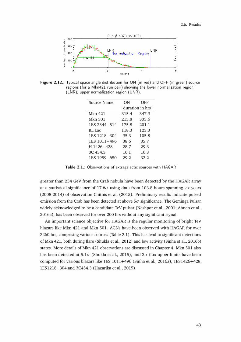
2.6. Results
Figure 2.12.: Typical space angle distribution for ON (in red) and OFF (in green) sourceregions (for a Mkn421 run pair) showing the lower normalisation region(LNR), upper normalization region (UNR).
Source Name ON OFF[duration in hrs]
Mkn 421 315.4 347.9Mkn 501 215.8 335.61ES 2344+514 175.8 201.1BL Lac 118.3 123.31ES 1218+304 95.3 105.81ES 1011+496 38.6 35.7H 1426+428 28.7 29.33C 454.3 16.1 16.31ES 1959+650 29.2 32.2
Table 2.1.: Observations of extragalactic sources with HAGAR
greater than 234 GeV from the Crab nebula have been detected by the HAGAR array
at a statistical significance of 17.6σ using data from 103.8 hours spanning six years
(2008-2014) of observation Chitnis et al. (2015). Preliminary results indicate pulsed
emission from the Crab has been detected at above 5σ significance. The Geminga Pulsar,
widely acknowledged to be a candidate TeV pulsar (Neshpor et al., 2001; Ahnen et al.,
2016a), has been observed for over 200 hrs without any significant signal.
An important science objective for HAGAR is the regular monitoring of bright TeV
blazars like Mkn 421 and Mkn 501. AGNs have been observed with HAGAR for over
2260 hrs, comprising various sources (Table 2.1). This has lead to significant detections
of Mkn 421, both during flare (Shukla et al., 2012) and low activity (Sinha et al., 2016b)
states. More details of Mkn 421 observations are discussed in Chapter 4. Mkn 501 also
has been detected at 5.1σ (Shukla et al., 2015), and 3σ flux upper limits have been
computed for various blazars like 1ES 1011+496 (Sinha et al., 2016a), 1ES1426+428,
1ES1218+304 and 3C454.3 (Hazarika et al., 2015).
43


“Theories crumble, but good observations never fade."
Harlow Shapey
3Multiwavelength Instrumentation and
Data Analysis
THE AIM OF THIS THESIS is to perform a multiwavelength study of TeV blazars to un-
derstand their broadband spectral and temporal properties, with emphasis on the high
energy emission. To this effect, we have used data from a variety of space and ground
based instruments, mostly available under the “Fermi Multiwavelength Observing Support
Program"1. A brief and compact description of the data, instruments and their analysis
procedures is given in the following sections, starting from the γ-rays and going down to
radio wavelengths.
3.1 F E R M I -L AT
The Fermi Gamma-ray Space Telescope (Fermi) spacecraft, formerly known as the Gamma-
ray Large Area Space Telescope (GLAST) was launched on June 11, 2008 into a low
earth orbit by NASA. The Fermi spacecraft carries two scientific payloads, the Large
Area Telescope (LAT) and the Gamma-ray Burst Monitor (GBM). While the LAT is the
principal instrument on board, the GBM, operating in the energy range of 8 keV to 40
MeV, complements the LAT in its observations of γ-ray transients. Details of the GBM can
be found in Meegan et al. (2009).
The LAT is a pair production telescope operating in the energy range of 20 MeV to over
300 GeV. It has a 4 x 4 modular design, each module made of a precision tracker and
calorimeter. The trackers comprise 18 layers of paired Silicon Strip Detector planes with
interleaved tungsten foils. These trackers measure the electron-positron tracks resulting
1 http://fermi.gsfc.nasa.gov/ssc/observations/multi/programs.html
45
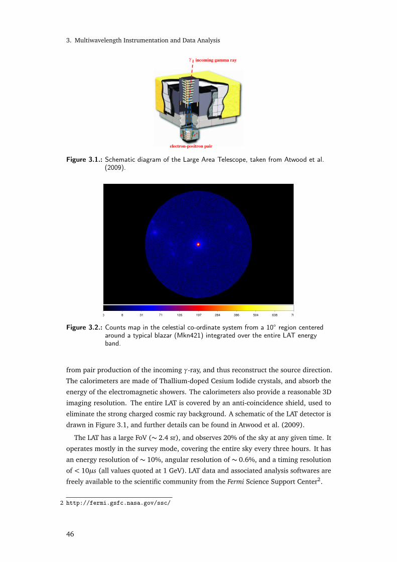
3. Multiwavelength Instrumentation and Data Analysis
Figure 3.1.: Schematic diagram of the Large Area Telescope, taken from Atwood et al.(2009).
0 8 31 71 126 197 284 386 504 638 787
Figure 3.2.: Counts map in the celestial co-ordinate system from a 10 region centeredaround a typical blazar (Mkn421) integrated over the entire LAT energyband.
from pair production of the incoming γ-ray, and thus reconstruct the source direction.
The calorimeters are made of Thallium-doped Cesium Iodide crystals, and absorb the
energy of the electromagnetic showers. The calorimeters also provide a reasonable 3D
imaging resolution. The entire LAT is covered by an anti-coincidence shield, used to
eliminate the strong charged cosmic ray background. A schematic of the LAT detector is
drawn in Figure 3.1, and further details can be found in Atwood et al. (2009).
The LAT has a large FoV (∼ 2.4 sr), and observes 20% of the sky at any given time. It
operates mostly in the survey mode, covering the entire sky every three hours. It has
an energy resolution of ∼ 10%, angular resolution of ∼ 0.6%, and a timing resolution
of < 10µs (all values quoted at 1 GeV). LAT data and associated analysis softwares are
freely available to the scientific community from the Fermi Science Support Center2.
2 http://fermi.gsfc.nasa.gov/ssc/
46

3.2. NuSTAR
Figure 3.3.: Schematic of the NuSTAR telescope, taken from Bhalerao (2012).
The LAT data used in this thesis are extracted from a region of 20 centered on the
source. The standard data analysis procedure as mentioned in the Fermi-LAT docu-
mentation3 is used. Events belonging to the energy range 0.2−300 GeV and SOURCE
class are used. Good time intervals are calculated from the spacecraft file by impos-
ing a filter “DATA_QUAL>0”, && “LAT_CONFIG==1”. Only events with less than 105
zenith angle are selected to avoid contamination from the Earth limb γ-rays. The
galactic diffuse emission component gll_iem_v05_rev1.fits and an isotropic component
iso_source_v05_rev1.txt are used as the background models. The unbinned likelihood
method included in the pylikelihood library of Science Tools (v9r33p0) and the
post-launch instrument response functions P7REP_SOURCE_V15 are used for the analy-
sis. All the sources lying within 10 region of interest (ROI) centered at the source and
defined in the third Fermi-LAT catalog (Acero et al., 2015), are included in the model xml
file. All the parameters except the scaling factor of the sources within the ROI are allowed
to vary during the likelihood fitting. For sources between 10 to 20 from the centre, all
parameters were kept frozen at the default values. Integrated Fermi-LAT counts map
centered on Mkn421 in shown in Figure 3.2.
3.2 N U S TA R
Launched in June 2012 under the NASA Small Explorer satellite program (SMEX-11), the
Nuclear Spectroscopic Telescope Array (NuSTAR) features the first space-based focussing
hard X-ray telescope. NuSTAR provides sub-arcminute imaging with excellent spectral
resolution in the 3 - 79 keV band over a 12-arcminute FoV, at a temporal resolution
of 2 µs. It consists of two co-aligned, depth-graded multilayer coated Wolter I conical
approximation X-ray optics which focus onto two independent solid-state focal plane
detectors. Each detector unit is comprised of four Cadmium-Zinc-Telluride (CdZnTe, or
CZT) detectors, and is surrounded by a CsI anti-coincidence shield to veto off-axis events.
3 http://fermi.gsfc.nasa.gov/ssc/data/analysis/documentation/
47

3. Multiwavelength Instrumentation and Data Analysis
Figure 3.4.: NuSTAR image of Mkn421 from a single observation showing the source (12pixels, in black) and background (40 pixels, in white) extraction regions.
A schematic diagram of the instrument is shown in Figure 3.3 and detailed description
of the electronics can be found in Harrison et al. (2013).
NuSTAR data available at the HEASARC data portal4 are downloaded and processed
with the NuSTARDAS software package v.1.4.1 available within HEASOFT package
(6.16). The latest CALDB (v.20140414) is used. After running nupipeline v.0.4.3on each observation, nuproducts v.0.2.8 is used to obtain the light curves and
spectra. Circular regions of 12 pixels centered on the source and of 40 pixels centered
on a source free region are used as source and background region respectively (Figure
3.4). Spectra from the two detectors A and B are combined using addascaspec. Data
from various observations are added using addascaspec and then grouped (using the
tool grppha) to ensure a minimum of 30 counts in each bin. Spectra are analyzed in
XSPEC simultaneous with Swift-XRT spectra.
3.3 S W I F T
The Swift satellite, launched on 20 November 2004 by NASA, is a multiwavelength
observatory with simultaneous observational capabilities from optical-UV to hard X-
ray energies. While mainly designed to study gamma ray bursts (GRB), the Swift has
also made huge advances in the field of blazars (Ghisellini, 2015).As shown in the
schematic diagram in Figure 3.5, it has three co-aligned instruments on board; the Burst
Alert Telescope (BAT), the X-ray Telescope (XRT), and the Ultraviolet/Optical Telescope
(UVOT).
4 http://heasarc.gsfc.nasa.gov/xamin/xamin.jsp
48
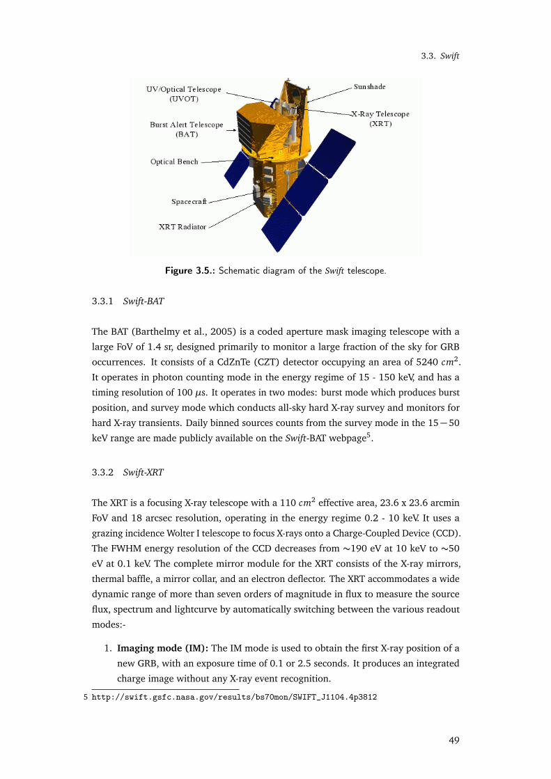
3.3. Swift
Figure 3.5.: Schematic diagram of the Swift telescope.
3.3.1 Swift-BAT
The BAT (Barthelmy et al., 2005) is a coded aperture mask imaging telescope with a
large FoV of 1.4 sr, designed primarily to monitor a large fraction of the sky for GRB
occurrences. It consists of a CdZnTe (CZT) detector occupying an area of 5240 cm2.
It operates in photon counting mode in the energy regime of 15 - 150 keV, and has a
timing resolution of 100 µs. It operates in two modes: burst mode which produces burst
position, and survey mode which conducts all-sky hard X-ray survey and monitors for
hard X-ray transients. Daily binned sources counts from the survey mode in the 15−50
keV range are made publicly available on the Swift-BAT webpage5.
3.3.2 Swift-XRT
The XRT is a focusing X-ray telescope with a 110 cm2 effective area, 23.6 x 23.6 arcmin
FoV and 18 arcsec resolution, operating in the energy regime 0.2 - 10 keV. It uses a
grazing incidence Wolter I telescope to focus X-rays onto a Charge-Coupled Device (CCD).
The FWHM energy resolution of the CCD decreases from ∼190 eV at 10 keV to ∼50
eV at 0.1 keV. The complete mirror module for the XRT consists of the X-ray mirrors,
thermal baffle, a mirror collar, and an electron deflector. The XRT accommodates a wide
dynamic range of more than seven orders of magnitude in flux to measure the source
flux, spectrum and lightcurve by automatically switching between the various readout
modes:-
1. Imaging mode (IM): The IM mode is used to obtain the first X-ray position of a
new GRB, with an exposure time of 0.1 or 2.5 seconds. It produces an integrated
charge image without any X-ray event recognition.
5 http://swift.gsfc.nasa.gov/results/bs70mon/SWIFT_J1104.4p3812
49

3. Multiwavelength Instrumentation and Data Analysis
Figure 3.6.: Windowed Timing (WT) and Photon Counting (PC) images of the sameblazar BL Lac from different observations.
2. Photo-Diode mode (PD): The PD mode used to provide a high speed light curve
with time resolution of 0.14ms for fluxes below 60 Crabs, without any spatial
resolution. This mode has been disabled since May 2005.
3. Photon-Counting mode (PC): The PC mode retains the full imaging and spectro-
scopic resolution of the instrument, but with a time resolution of 2.5 seconds. This
is used for low count rates (below 10 mCrab).
4. Windowed Timing mode (WT): The WT is a high gain mode which produces a
full spectral resolution, high timing resolution of 1.7 ms, but a 1-dim image. This
is used for high count rates (over 10 mCrab).
Examples of WT (of Mkn421) and PC (of BL Lac) images are shown in Figure 3.6.
Further details about the XRT instrumentation can be found in Burrows et al. (2005).
The XRT data used in the present work are downloaded from the HEASARC data portal
and processed with the XRTDAS software package (v.3.0.0) available within HEASOFT
package (6.16). Latest calibration files from the Swift CALDB are used. Observations are
available both in WT and PC modes, and full grade selections (0-2 for WT; 0-12 for PC) are
used. Event files are cleaned and calibrated using standard procedures (xrtpipeline),
and xrtproducts is used to obtain the light curves and spectra. Circular regions of
20 pixels centred on the source and of 40 pixels from a source-free region are used as
source and background regions respectively.
Many of the observations are significantly affected by pileup (count rate > 100
cts/s(WT); > 0.5 cts/s(PC) ) (Romano et al., 2006), and is corrected for by following
the procedure outlined in the Swift analysis threads6. For the PC mode, the XRT Point
Spread Function is modelled by a King function
PSF(r) = [1+(r/rc)2]−β (39)
with rc = 5.8 and β = 1.55 (Moretti et al., 2005). Depending on the source brightness,
annular regions are chosen to exclude pixels deviating from the King’s function. For eg,
6 http://www.swift.ac.uk/analysis/xrt/pileup.php
50
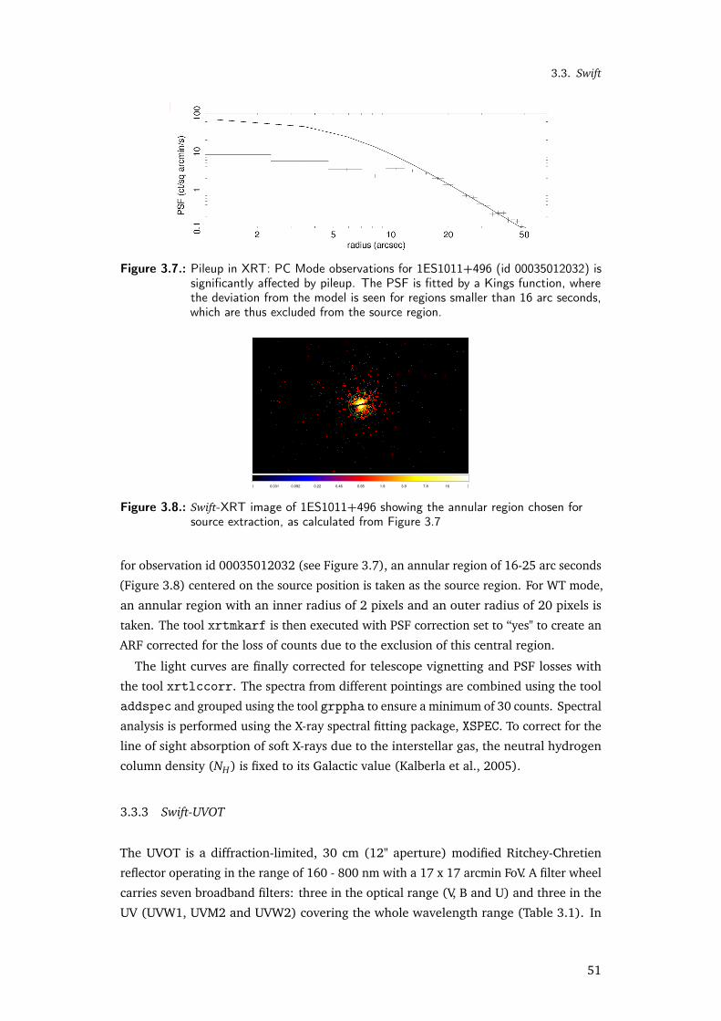
3.3. Swift
Figure 3.7.: Pileup in XRT: PC Mode observations for 1ES1011+496 (id 00035012032) issignificantly affected by pileup. The PSF is fitted by a Kings function, wherethe deviation from the model is seen for regions smaller than 16 arc seconds,which are thus excluded from the source region.
0 0.031 0.092 0.22 0.46 0.95 1.9 3.9 7.8 16 31
Figure 3.8.: Swift-XRT image of 1ES1011+496 showing the annular region chosen forsource extraction, as calculated from Figure 3.7
for observation id 00035012032 (see Figure 3.7), an annular region of 16-25 arc seconds
(Figure 3.8) centered on the source position is taken as the source region. For WT mode,
an annular region with an inner radius of 2 pixels and an outer radius of 20 pixels is
taken. The tool xrtmkarf is then executed with PSF correction set to “yes" to create an
ARF corrected for the loss of counts due to the exclusion of this central region.
The light curves are finally corrected for telescope vignetting and PSF losses with
the tool xrtlccorr. The spectra from different pointings are combined using the tool
addspec and grouped using the tool grppha to ensure a minimum of 30 counts. Spectral
analysis is performed using the X-ray spectral fitting package, XSPEC. To correct for the
line of sight absorption of soft X-rays due to the interstellar gas, the neutral hydrogen
column density (NH) is fixed to its Galactic value (Kalberla et al., 2005).
3.3.3 Swift-UVOT
The UVOT is a diffraction-limited, 30 cm (12" aperture) modified Ritchey-Chretien
reflector operating in the range of 160 - 800 nm with a 17 x 17 arcmin FoV. A filter wheel
carries seven broadband filters: three in the optical range (V, B and U) and three in the
UV (UVW1, UVM2 and UVW2) covering the whole wavelength range (Table 3.1). In
51
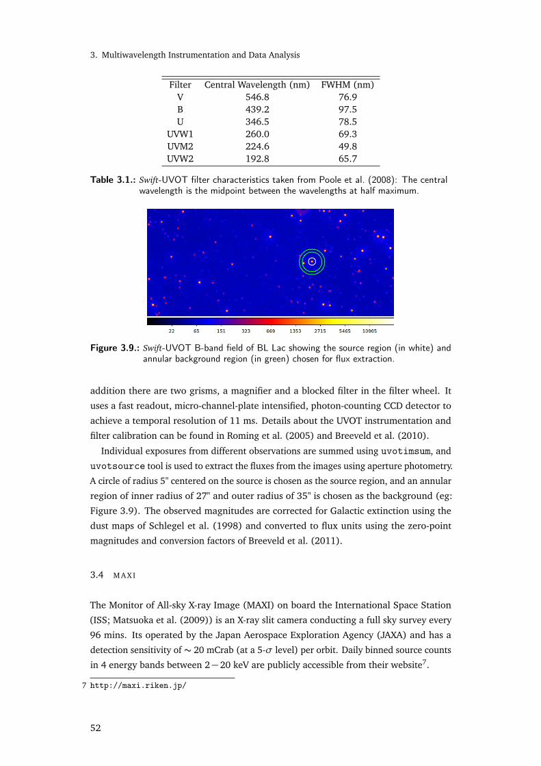
3. Multiwavelength Instrumentation and Data Analysis
Filter Central Wavelength (nm) FWHM (nm)V 546.8 76.9B 439.2 97.5U 346.5 78.5
UVW1 260.0 69.3UVM2 224.6 49.8UVW2 192.8 65.7
Table 3.1.: Swift-UVOT filter characteristics taken from Poole et al. (2008): The centralwavelength is the midpoint between the wavelengths at half maximum.
Figure 3.9.: Swift-UVOT B-band field of BL Lac showing the source region (in white) andannular background region (in green) chosen for flux extraction.
addition there are two grisms, a magnifier and a blocked filter in the filter wheel. It
uses a fast readout, micro-channel-plate intensified, photon-counting CCD detector to
achieve a temporal resolution of 11 ms. Details about the UVOT instrumentation and
filter calibration can be found in Roming et al. (2005) and Breeveld et al. (2010).
Individual exposures from different observations are summed using uvotimsum, and
uvotsource tool is used to extract the fluxes from the images using aperture photometry.
A circle of radius 5" centered on the source is chosen as the source region, and an annular
region of inner radius of 27" and outer radius of 35" is chosen as the background (eg:
Figure 3.9). The observed magnitudes are corrected for Galactic extinction using the
dust maps of Schlegel et al. (1998) and converted to flux units using the zero-point
magnitudes and conversion factors of Breeveld et al. (2011).
3.4 M A X I
The Monitor of All-sky X-ray Image (MAXI) on board the International Space Station
(ISS; Matsuoka et al. (2009)) is an X-ray slit camera conducting a full sky survey every
96 mins. Its operated by the Japan Aerospace Exploration Agency (JAXA) and has a
detection sensitivity of ∼ 20 mCrab (at a 5-σ level) per orbit. Daily binned source counts
in 4 energy bands between 2−20 keV are publicly accessible from their website7.
7 http://maxi.riken.jp/
52
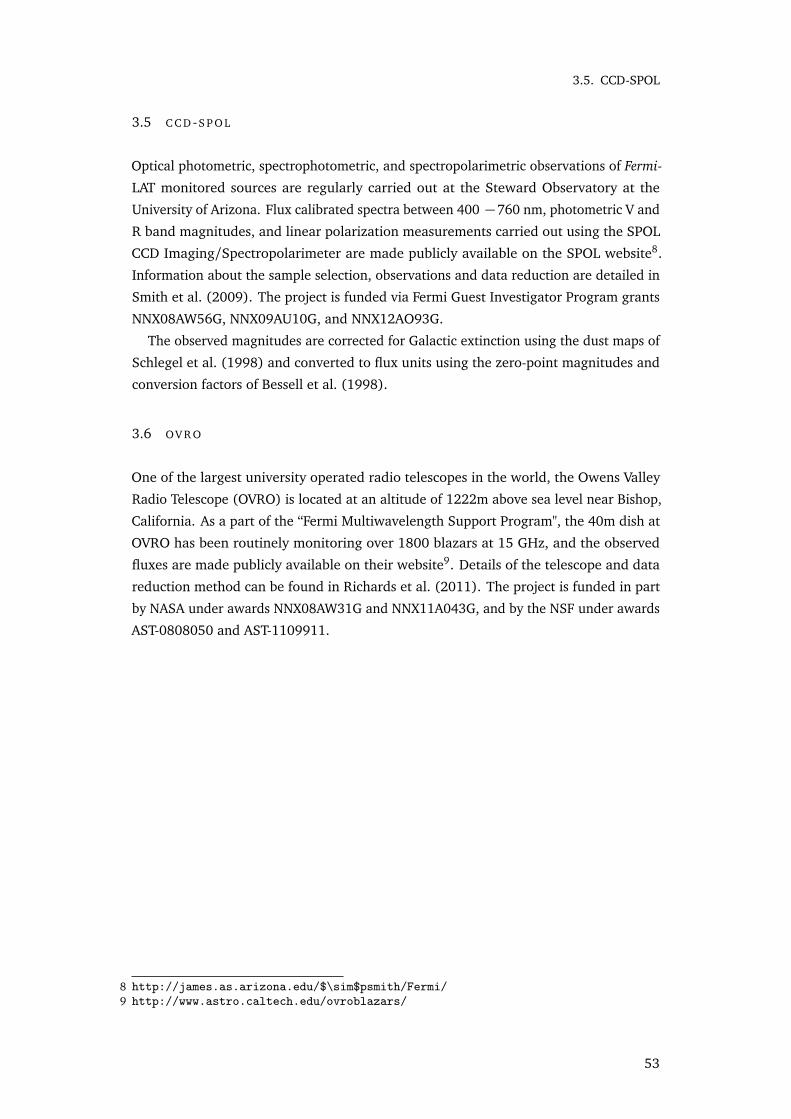
3.5. CCD-SPOL
3.5 C C D -S P O L
Optical photometric, spectrophotometric, and spectropolarimetric observations of Fermi-
LAT monitored sources are regularly carried out at the Steward Observatory at the
University of Arizona. Flux calibrated spectra between 400 −760 nm, photometric V and
R band magnitudes, and linear polarization measurements carried out using the SPOL
CCD Imaging/Spectropolarimeter are made publicly available on the SPOL website8.
Information about the sample selection, observations and data reduction are detailed in
Smith et al. (2009). The project is funded via Fermi Guest Investigator Program grants
NNX08AW56G, NNX09AU10G, and NNX12AO93G.
The observed magnitudes are corrected for Galactic extinction using the dust maps of
Schlegel et al. (1998) and converted to flux units using the zero-point magnitudes and
conversion factors of Bessell et al. (1998).
3.6 OV R O
One of the largest university operated radio telescopes in the world, the Owens Valley
Radio Telescope (OVRO) is located at an altitude of 1222m above sea level near Bishop,
California. As a part of the “Fermi Multiwavelength Support Program", the 40m dish at
OVRO has been routinely monitoring over 1800 blazars at 15 GHz, and the observed
fluxes are made publicly available on their website9. Details of the telescope and data
reduction method can be found in Richards et al. (2011). The project is funded in part
by NASA under awards NNX08AW31G and NNX11A043G, and by the NSF under awards
AST-0808050 and AST-1109911.
8 http://james.as.arizona.edu/$\sim$psmith/Fermi/9 http://www.astro.caltech.edu/ovroblazars/
53


“Patience is bitter, but its fruit is sweet."
Aristotle
4Mkn 421: Longterm spectral and
temporal study
THE NEARBY AND THE MOST WELL STUDIED BLAZAR, MARKARAIN 421 has been the subject
of several multiwavelength campaigns both during flare and quiescent states. In 1992,
the Whipple collaboration reported the discovery of Mkn 421 (RA: 11 04’ 27.3"; Dec:
38 12’ 32"; z = 0.031) (Punch et al., 1992), making this the first extragalactic source
detected at TeV energies. It is one of the brightest BL Lac objects seen in the UV/X-ray/γ-
ray bands, thus making it an ideal candidate for both longterm statistical studies and
short term high cadence observations during its numerous flares. In this chapter we
report on the long term study of Mkn 421 carried out with the HAGAR telescope array
during 2009-2015 (Sinha et al., 2016b), while in the next chapter we describe the largest
X-ray flare seen from this source in the past decade (Sinha et al., 2015).
4.1 B R I E F R E V I E W O F PA S T R E S U LT S
Apart from being the first detected TeV blazar, Mkn 421 has a rich and interesting history
of paving the way forward in many different wavebands. Mkn 421 was identified with the
radio galaxy B2 1101+38 in the year 1975 by Ulrich et al. (1975). It was shown to have
a featureless, non-thermal, but highly polarised optical spectrum, leading to a conclusion
that Mrk 421 is a normal elliptical galaxy with a central, compact, non-thermal nucleus,
quite similar to the source BL Lacertae (BL Lac). Soon, Ricketts et al. (1976), discovered
a highly variable soft X-ray component from this source using data from the Arial V
satellite. This was the first time a BL Lac object was associated with an X-ray source. It
is also the first BL Lac object to be detected by the Energetic Gamma Ray Experiment
55
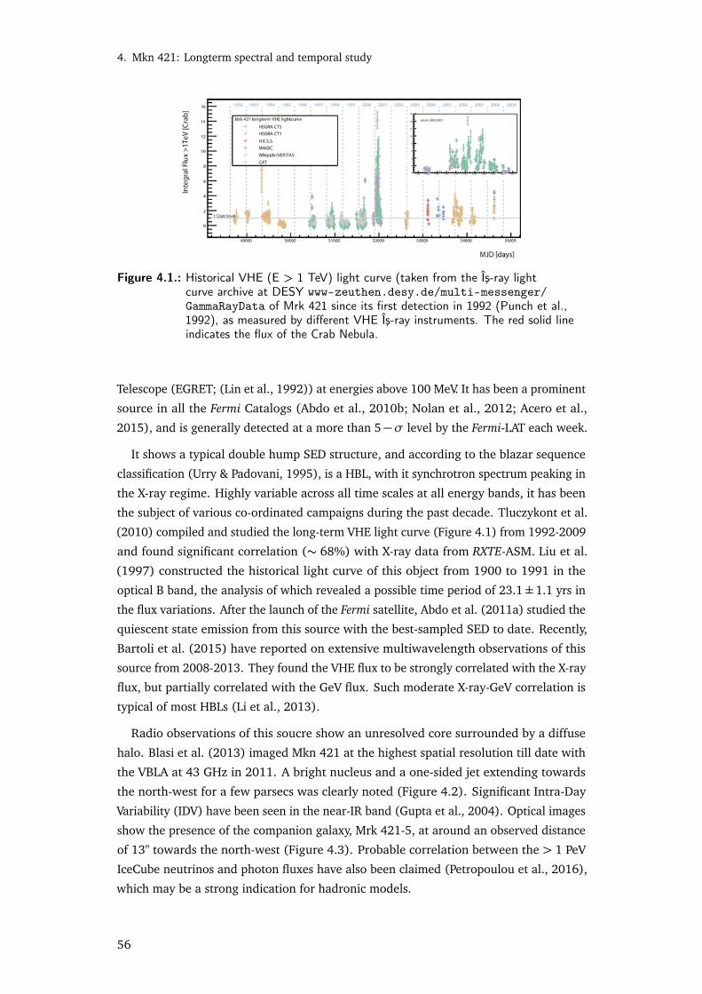
4. Mkn 421: Longterm spectral and temporal study
Figure 4.1.: Historical VHE (E > 1 TeV) light curve (taken from the Îş-ray lightcurve archive at DESY www-zeuthen.desy.de/multi-messenger/GammaRayData of Mrk 421 since its first detection in 1992 (Punch et al.,1992), as measured by different VHE Îş-ray instruments. The red solid lineindicates the flux of the Crab Nebula.
Telescope (EGRET; (Lin et al., 1992)) at energies above 100 MeV. It has been a prominent
source in all the Fermi Catalogs (Abdo et al., 2010b; Nolan et al., 2012; Acero et al.,
2015), and is generally detected at a more than 5−σ level by the Fermi-LAT each week.
It shows a typical double hump SED structure, and according to the blazar sequence
classification (Urry & Padovani, 1995), is a HBL, with it synchrotron spectrum peaking in
the X-ray regime. Highly variable across all time scales at all energy bands, it has been
the subject of various co-ordinated campaigns during the past decade. Tluczykont et al.
(2010) compiled and studied the long-term VHE light curve (Figure 4.1) from 1992-2009
and found significant correlation (∼ 68%) with X-ray data from RXTE-ASM. Liu et al.
(1997) constructed the historical light curve of this object from 1900 to 1991 in the
optical B band, the analysis of which revealed a possible time period of 23.1±1.1 yrs in
the flux variations. After the launch of the Fermi satellite, Abdo et al. (2011a) studied the
quiescent state emission from this source with the best-sampled SED to date. Recently,
Bartoli et al. (2015) have reported on extensive multiwavelength observations of this
source from 2008-2013. They found the VHE flux to be strongly correlated with the X-ray
flux, but partially correlated with the GeV flux. Such moderate X-ray-GeV correlation is
typical of most HBLs (Li et al., 2013).
Radio observations of this soucre show an unresolved core surrounded by a diffuse
halo. Blasi et al. (2013) imaged Mkn 421 at the highest spatial resolution till date with
the VBLA at 43 GHz in 2011. A bright nucleus and a one-sided jet extending towards
the north-west for a few parsecs was clearly noted (Figure 4.2). Significant Intra-Day
Variability (IDV) have been seen in the near-IR band (Gupta et al., 2004). Optical images
show the presence of the companion galaxy, Mrk 421-5, at around an observed distance
of 13" towards the north-west (Figure 4.3). Probable correlation between the > 1 PeV
IceCube neutrinos and photon fluxes have also been claimed (Petropoulou et al., 2016),
which may be a strong indication for hadronic models.
56

4.1. Brief review of past results
MilliA
RC
SE
C
MilliARC SEC
1 0 -1 -2 -3 -4
4
3
2
1
0
-1
Figure 4.2.: VLBA image of Mkn 421 at 43 GHz corresponding to April 2013 observationof the Boston University monitoring program (Blasi et al., 2013)
Figure 4.3.: Optical R-band image (size 78" by 78") of Mkn 421 as seen by the NordicOptical Telescope (Nilsson et al., 1999). The companion galaxy Mrk 421-5can be clearly seen in the north-west.
57
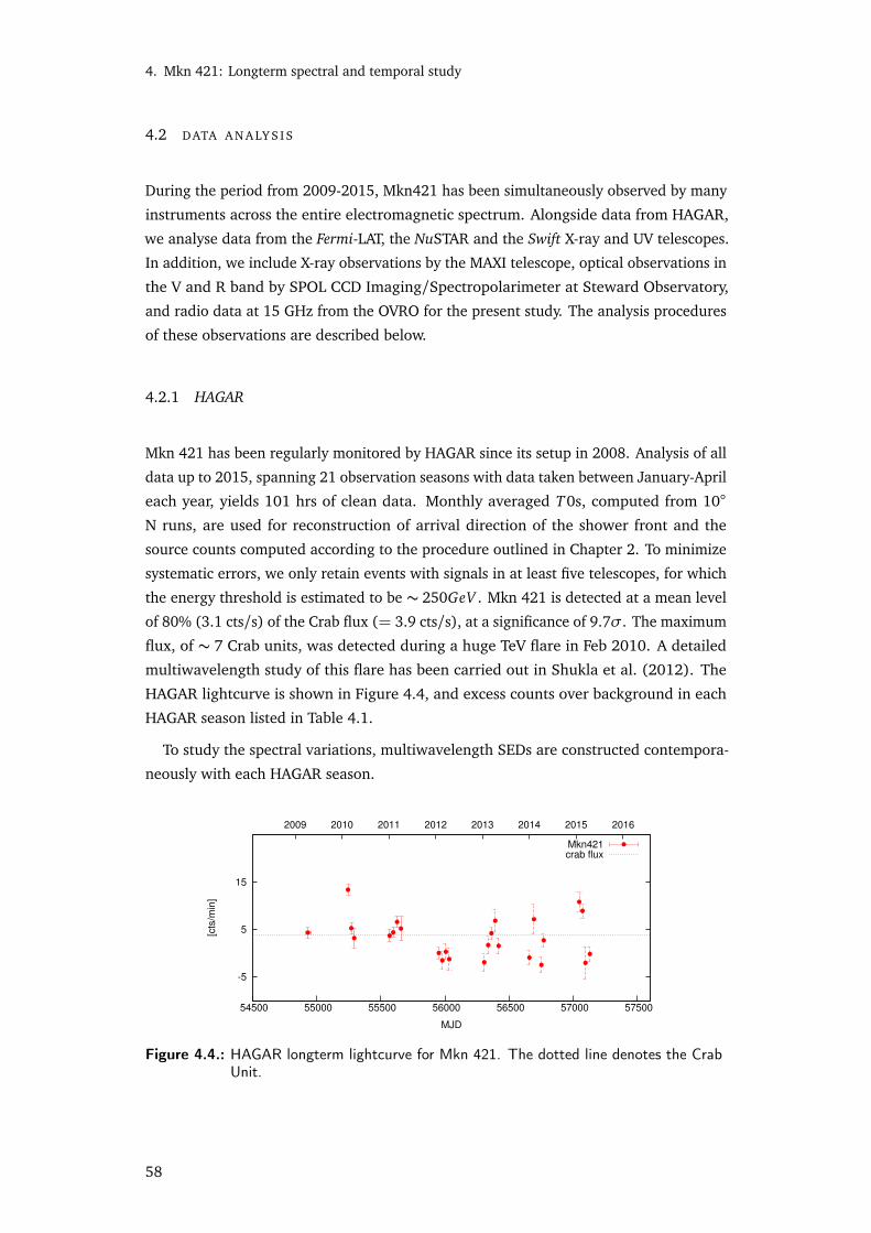
4. Mkn 421: Longterm spectral and temporal study
4.2 DATA A N A LY S I S
During the period from 2009-2015, Mkn421 has been simultaneously observed by many
instruments across the entire electromagnetic spectrum. Alongside data from HAGAR,
we analyse data from the Fermi-LAT, the NuSTAR and the Swift X-ray and UV telescopes.
In addition, we include X-ray observations by the MAXI telescope, optical observations in
the V and R band by SPOL CCD Imaging/Spectropolarimeter at Steward Observatory,
and radio data at 15 GHz from the OVRO for the present study. The analysis procedures
of these observations are described below.
4.2.1 HAGAR
Mkn 421 has been regularly monitored by HAGAR since its setup in 2008. Analysis of all
data up to 2015, spanning 21 observation seasons with data taken between January-April
each year, yields 101 hrs of clean data. Monthly averaged T0s, computed from 10
N runs, are used for reconstruction of arrival direction of the shower front and the
source counts computed according to the procedure outlined in Chapter 2. To minimize
systematic errors, we only retain events with signals in at least five telescopes, for which
the energy threshold is estimated to be ∼ 250GeV . Mkn 421 is detected at a mean level
of 80% (3.1 cts/s) of the Crab flux (= 3.9 cts/s), at a significance of 9.7σ. The maximum
flux, of ∼ 7 Crab units, was detected during a huge TeV flare in Feb 2010. A detailed
multiwavelength study of this flare has been carried out in Shukla et al. (2012). The
HAGAR lightcurve is shown in Figure 4.4, and excess counts over background in each
HAGAR season listed in Table 4.1.
To study the spectral variations, multiwavelength SEDs are constructed contempora-
neously with each HAGAR season.
-5
5
15
54500 55000 55500 56000 56500 57000 57500
2009 2010 2011 2012 2013 2014 2015 2016
[cts
/min
]
MJD
Mkn421crab flux
Figure 4.4.: HAGAR longterm lightcurve for Mkn 421. The dotted line denotes the CrabUnit.
58
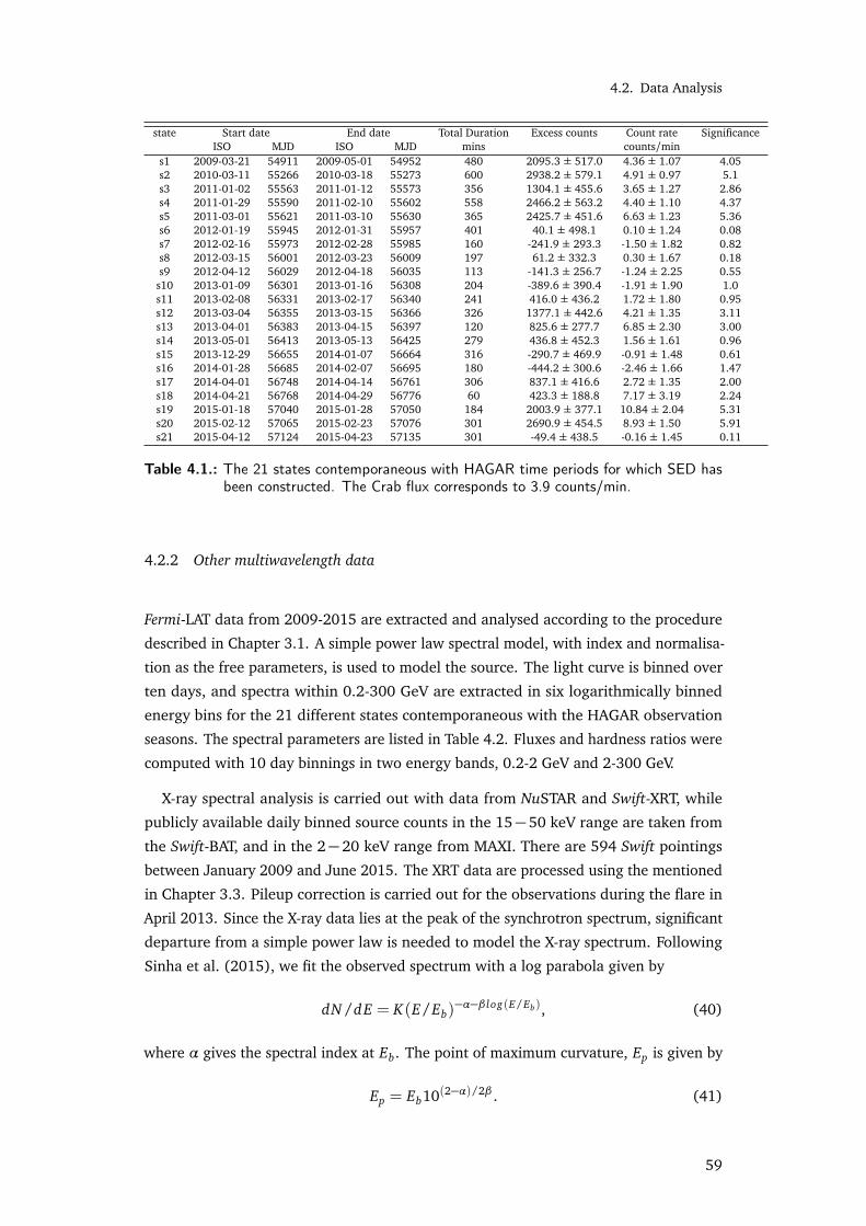
4.2. Data Analysis
state Start date End date Total Duration Excess counts Count rate SignificanceISO MJD ISO MJD mins counts/min
s1 2009-03-21 54911 2009-05-01 54952 480 2095.3 ± 517.0 4.36 ± 1.07 4.05s2 2010-03-11 55266 2010-03-18 55273 600 2938.2 ± 579.1 4.91 ± 0.97 5.1s3 2011-01-02 55563 2011-01-12 55573 356 1304.1 ± 455.6 3.65 ± 1.27 2.86s4 2011-01-29 55590 2011-02-10 55602 558 2466.2 ± 563.2 4.40 ± 1.10 4.37s5 2011-03-01 55621 2011-03-10 55630 365 2425.7 ± 451.6 6.63 ± 1.23 5.36s6 2012-01-19 55945 2012-01-31 55957 401 40.1 ± 498.1 0.10 ± 1.24 0.08s7 2012-02-16 55973 2012-02-28 55985 160 -241.9 ± 293.3 -1.50 ± 1.82 0.82s8 2012-03-15 56001 2012-03-23 56009 197 61.2 ± 332.3 0.30 ± 1.67 0.18s9 2012-04-12 56029 2012-04-18 56035 113 -141.3 ± 256.7 -1.24 ± 2.25 0.55s10 2013-01-09 56301 2013-01-16 56308 204 -389.6 ± 390.4 -1.91 ± 1.90 1.0s11 2013-02-08 56331 2013-02-17 56340 241 416.0 ± 436.2 1.72 ± 1.80 0.95s12 2013-03-04 56355 2013-03-15 56366 326 1377.1 ± 442.6 4.21 ± 1.35 3.11s13 2013-04-01 56383 2013-04-15 56397 120 825.6 ± 277.7 6.85 ± 2.30 3.00s14 2013-05-01 56413 2013-05-13 56425 279 436.8 ± 452.3 1.56 ± 1.61 0.96s15 2013-12-29 56655 2014-01-07 56664 316 -290.7 ± 469.9 -0.91 ± 1.48 0.61s16 2014-01-28 56685 2014-02-07 56695 180 -444.2 ± 300.6 -2.46 ± 1.66 1.47s17 2014-04-01 56748 2014-04-14 56761 306 837.1 ± 416.6 2.72 ± 1.35 2.00s18 2014-04-21 56768 2014-04-29 56776 60 423.3 ± 188.8 7.17 ± 3.19 2.24s19 2015-01-18 57040 2015-01-28 57050 184 2003.9 ± 377.1 10.84 ± 2.04 5.31s20 2015-02-12 57065 2015-02-23 57076 301 2690.9 ± 454.5 8.93 ± 1.50 5.91s21 2015-04-12 57124 2015-04-23 57135 301 -49.4 ± 438.5 -0.16 ± 1.45 0.11
Table 4.1.: The 21 states contemporaneous with HAGAR time periods for which SED hasbeen constructed. The Crab flux corresponds to 3.9 counts/min.
4.2.2 Other multiwavelength data
Fermi-LAT data from 2009-2015 are extracted and analysed according to the procedure
described in Chapter 3.1. A simple power law spectral model, with index and normalisa-
tion as the free parameters, is used to model the source. The light curve is binned over
ten days, and spectra within 0.2-300 GeV are extracted in six logarithmically binned
energy bins for the 21 different states contemporaneous with the HAGAR observation
seasons. The spectral parameters are listed in Table 4.2. Fluxes and hardness ratios were
computed with 10 day binnings in two energy bands, 0.2-2 GeV and 2-300 GeV.
X-ray spectral analysis is carried out with data from NuSTAR and Swift-XRT, while
publicly available daily binned source counts in the 15−50 keV range are taken from
the Swift-BAT, and in the 2− 20 keV range from MAXI. There are 594 Swift pointings
between January 2009 and June 2015. The XRT data are processed using the mentioned
in Chapter 3.3. Pileup correction is carried out for the observations during the flare in
April 2013. Since the X-ray data lies at the peak of the synchrotron spectrum, significant
departure from a simple power law is needed to model the X-ray spectrum. Following
Sinha et al. (2015), we fit the observed spectrum with a log parabola given by
dN/dE = K(E/Eb)−α−β log(E/Eb), (40)
where α gives the spectral index at Eb. The point of maximum curvature, Ep is given by
Ep = Eb10(2−α)/2β . (41)
59
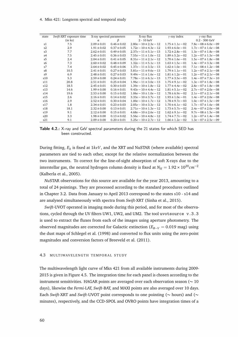
4. Mkn 421: Longterm spectral and temporal study
state Swift-XRT exposure time X-ray spectral parameters X-ray flux γ-ray index γ-ray flux(in ks) α β 2 - 10 keV 0.2 - 300 GeV
s1 7.5 2.09±0.01 0.46±0.02 2.80e−10±2.3e−12 1.75±1.1e−02 7.8e−08±6.0e−09s2 2.9 1.91±0.02 0.37±0.05 1.72e−10±4.3e−12 1.93±6.0e−01 1.7e−07±1.6e−08s3 7.7 2.62±0.01 0.49±0.05 2.37e−11±5.1e−13 1.72±2.8e−01 1.3e−07±1.8e−08s4 7.5 2.45±0.01 0.36±0.03 7.55e−11±1.0e−12 1.89±5.2e−02 1.2e−07±1.5e−08s5 2.4 2.04±0.01 0.41±0.05 8.31e−11±2.1e−12 1.70±1.6e−01 1.5e−07±1.8e−08s6 7.3 2.60±0.02 0.48±0.09 1.32e−11±5.1e−13 1.63±1.5e−01 1.4e−07±3.3e−08s7 7.4 2.64±0.02 0.45±0.06 1.37e−11±3.5e−13 1.62±1.0e−01 7.1e−08±1.2e−08s8 10.5 2.41±0.01 0.27±0.03 5.81e−11±9.6e−13 1.79±1.1e−01 1.2e−07±2.1e−08s9 6.9 2.48±0.01 0.27±0.03 9.49e−11±1.6e−12 1.81±1.2e−01 1.2e−07±2.1e−08s10 5.3 2.59±0.00 0.24±0.01 7.78e−11±6.1e−13 1.77±3.5e−03 1.4e−07±7.3e−10s11 20.8 2.51±0.01 0.25±0.04 1.96e−11±3.0e−13 1.75±9.1e−02 1.3e−07±1.8e−08s12 18.5 2.45±0.01 0.30±0.03 1.39e−10±1.8e−12 1.77±4.4e−02 2.8e−07±1.8e−08s13 14.6 1.99±0.00 0.16±0.01 9.43e−10±4.4e−12 1.81±5.1e−02 2.7e−07±2.0e−08s14 19.6 2.53±0.00 0.15±0.02 1.06e−10±1.0e−12 1.78±6.9e−02 2.1e−07±2.1e−08s15 2.6 2.16±0.01 0.14±0.02 3.33e−10±3.7e−12 1.93±1.0e−01 1.4e−07±2.0e−08s16 2.9 2.52±0.01 0.30±0.04 1.00e−10±1.7e−12 1.78±9.7e−03 1.0e−07±1.5e−09s17 1.8 2.34±0.01 0.23±0.03 2.05e−10±3.3e−12 1.70±6.1e−02 1.7e−07±1.6e−08s18 18.1 2.32±0.00 0.13±0.01 2.71e−10±1.3e−12 1.73±5.7e−02 2.4e−07±2.0e−08s19 9.1 2.12±0.00 0.15±0.01 4.68e−10±2.6e−12 1.62±9.1e−02 9.7e−08±1.5e−08s20 3.3 1.98±0.00 0.13±0.02 5.56e−10±4.8e−12 1.74±7.7e−02 1.2e−07±1.4e−08s21 9.1 2.09±0.00 0.20±0.01 5.25e−10±2.7e−12 1.66±1.2e−02 1.3e−07±2.5e−09
Table 4.2.: X-ray and GeV spectral parameters during the 21 states for which SED hasbeen constructed.
During fitting, Eb is fixed at 1keV , and the XRT and NuSTAR (where available) spectral
parameters are tied to each other, except for the relative normalization between the
two instruments. To correct for the line-of-sight absorption of soft X-rays due to the
interstellar gas, the neutral hydrogen column density is fixed at NH = 1.92×1020cm−2
(Kalberla et al., 2005).
NuSTAR observations for this source are available for the year 2013, amounting to a
total of 24 pointings. They are processed according to the standard procedures outlined
in Chapter 3.2. Data from January to April 2013 correspond to the states s10 - s14 and
are analysed simultaneously with spectra from Swift-XRT (Sinha et al., 2015).
Swift-UVOT operated in imaging mode during this period, and for most of the observa-
tions, cycled through the UV filters UW1, UW2, and UM2. The tool uvotsource v.3.3is used to extract the fluxes from each of the images using aperture photometry. The
observed magnitudes are corrected for Galactic extinction (EB−V = 0.019 mag) using
the dust maps of Schlegel et al. (1998) and converted to flux units using the zero-point
magnitudes and conversion factors of Breeveld et al. (2011).
4.3 M U LT I WAV E L E N GT H T E M P O R A L S T U DY
The multiwavelength light curve of Mkn 421 from all available instruments during 2009-
2015 is given in Figure 4.5. The integration time for each panel is chosen according to the
instrument sensitivities. HAGAR points are averaged over each observation season (∼ 10
days), likewise the Fermi-LAT, Swift-BAT, and MAXI points are also averaged over 10 days.
Each Swift-XRT and Swift-UVOT point corresponds to one pointing (∼ hours) and (∼minutes), respectively, and the CCD-SPOL and OVRO points have integration times of a
60
4.3. Multiwavelength temporal study
few seconds. As can be clearly seen, the source is variable across all wavelengths and
many flares can be identified. The most dramatic flare in the GeV band occurred during
in 2012 (MJD ∼ 56140−56180; calendar dates 2012-08-01 to 2012-09-10), which is
reflected in the radio band after a gap of one and half months (MJD ∼ 56193, Calendar
date 2012-09-23). In contrast, the largest X-ray/optical flare happened during April
2013, which has been studied in detail by various authors (Sinha et al., 2015; Pian et al.,
2014; Paliya et al., 2015a). In this section, we study the flux correlations between the
various frequencies and quantify the nature of the variability.
4.3.1 Variability and correlations
We quantify the variability using the fractional variability amplitude parameter Fvar
(Vaughan et al., 2003; Chitnis et al., 2009). It is calculated as
Fvar =
√
√S2−σ2er r
x2, (42)
where σ2er r is the mean square error, x the unweighted sample mean, and S2 the sample
variance. The error on Fvar is given as
σFvar=
√
√
√
√
√
√ 12N·σ2
er r
x2Fvar
2
+
√
√σ2er r
N·
1x
!2
. (43)
Here, N is the number of points.
The Fvar values derived from the light curves in Figure 4.5 are plotted in Figure 4.6. To
investigate the dependence of variability on the range of timescales, Fvar was computed
with 1-day, 10-day, 30-day and 3-month binning (Table 4.3). Owing to sensitivity issues,
Fvar at daily binning cannot be computed for γ-rays, i.e, with the Fermi-LAT and HAGAR.
The results remained roughly similar with differences showing up mainly in the X-ray
bands. For the optical/GeV bands, the difference is ∼ 5%. This shows that the low
variability seen in the optical/GeV bands is not an artifact of the binning, but is intrinsic
to the source. The variability is maximum in the X-ray/VHE bands, ∼ 80%/∼ 100%,
and goes down with frequency. The GeV and UV data show a similar variability index of
∼ 40%, which suggests a similar origin for the X-ray and VHE, and for the UV and GeV
spectrum. Similar results have been reported in Aleksic et al. (2014a).
We compute the hardness ratios from Swift-XRT data, which are defined as the ratio of
the flux in the 2−10 keV band to the flux in 0.3−2 keV band. As can be seen in Figure
4.7, while there is clear trend of spectral hardening with flux seen in the X-ray band
(ρ = 0.83, prob = 2.1×10⁻¹⁶), no such evidence is seen in the γ-ray band (ρ = 0.06
prob=0.33), again suggesting different origin for the X-ray and GeV data.
To study the lags between the various unevenly sampled energy bands, we use the
z-transformed discrete cross correlation function, freely available as a FORTRAN 90
61

4. Mkn 421: Longterm spectral and temporal study
0.5
1
[Jy]
OVRO
0.03
0.06
[Jy]
Optical V
4
12
50
150
[%]
[degre
e]
Pol deg
Pol angle
5
25
[mJy]
UV UW2
50
150
[cts
/s]
Swift-XRT
0.05
0.2
[cts
/s]
MAXI
2
8
[10
- 3 c
ts/s
]
Swift-BAT
2
6
[10
- 7 p
h/c
m2/s
]
Fermi-LAT
0
15
54500 55000 55500 56000 56500 57000
[cts
/min
]
MJD
HAGAR
Figure 4.5.: Multiwavelength light curve of Mkn421 from 2009-2015 showing in panel 1:radio fluxes at 15GHz from the OVRO; panel 2: optical V-band flux fromthe CCD-SPOL; panel 3: degree and angle of the optical polarization usingdata from CCD-SPOL; and panel 4: UV flux in the Swift-UVOT UW2 band.Fluxes in the UW1 and WM2 bands follow a similar trend, and thus onlyone band has been plotted to avoid cluttering. Panel 5: Swift-XRT countrates; panel 6: MAXI count rate (averaged over 10 days); panel 7 :Swift-BATcount rates (10 days averaged); panel 8:Fermi-LAT flux in 10−7ph/cm2/secaveraged over ten days; and panel 9: HAGAR counts/min, averaged overeach observation season. The black dotted line denotes the Crab count rate.
62

4.3. Multiwavelength temporal study
0
0.2
0.4
0.6
0.8
1
1.2
1.4
1e+10 1e+12 1e+14 1e+16 1e+18 1e+20 1e+22 1e+24 1e+26 1e+28
Fva
r
Frequency [Hz]
OVROOptical ROptical V
UW1UW2UM2
MAXIXRTBAT
Fermi 0.2-2GeVFermi 2-300GeV
HAGAR
Figure 4.6.: Fractional variability Fvar as a function of frequency.
Time BinningWaveband 1 day 10 days 1 month 3 monthsOVRO (15GHz) 0.22±0.01 0.20±0.01 0.19±0.01 0.19±0.01Optical R 0.32±0.01 0.31±0.01 0.31±0.01 0.29±0.02Optical V 0.37±0.01 0.36±0.01 0.37±0.01 0.35±0.02UV UW1 0.44±0.01 0.39±0.02 0.37±0.01 0.37±0.03UV UM2 0.47±0.01 0.42±0.02 0.41±0.02 0.40±0.03UV UW2 0.48±0.01 0.43±0.03 0.40±0.03 0.41±0.03Swift-XRT (0.2-10keV) 0.71±0.01 0.61±0.04 0.57±0.04 0.54±0.03MAXI (2-20keV) 0.81±0.01 0.79±0.10 0.74±0.08 0.67±0.02Swift-BAT (15-150keV) 1.08±0.01 0.95±0.16 0.90±0.10 0.81±0.04Fermi-LAT (0.2-2GeV) − 0.44±0.08 0.41±0.06 0.38±0.05Fermi-LAT (2-300GeV) − 0.48±0.14 0.42±0.08 0.38±0.07HAGAR ( > 200GeV) − 1.07±0.24 1.07±0.24 −
Table 4.3.: Fractional variability (Fvar) in different wavebands with different time binnings.
0
0.05
0.1
0.15
0.2
0.25
0.3
0.35
0.4
0.45
1 10 100 1000
Hard
ne
ss r
atio
Count rate 0.3-2 keV [cts/sec]
Swift-XRT
(a) Swift-XRT
0
0.05
0.1
0.15
0.2
0.25
0.3
1e-08 1e-07 1e-06
Hard
ness r
atio
Flux 0.2-2 GeV [ph/cm2/sec]
Fermi-LAT
(b) Fermi-LAT
Figure 4.7.: Hardness ratio in the X-ray (Swift-XRT) and GeV (Fermi-LAT) bands. Whilethe trend of spectral hardening with flux is clear in the X-ray band, no such trend isseen in the GeV band.
63

4. Mkn 421: Longterm spectral and temporal study
-1
-0.5
0
0.5
1
-400 -200 0 200 400
z-D
CF
Lag [days]
Fermi low-highMAXI - Swift-BAT
(a) Low- and high-energy X-rays (blue),and low- and high-energy bands inFermi (red)
-1
-0.5
0
0.5
1
-400 -200 0 200 400
z-D
CF
Lag [days]
Swift-BAT - FermiSwift-XRT - Fermi
(b) Swift-BAT and Fermi-LAT (blue),Swift-XRT and Fermi-LAT (red)
-1
-0.5
0
0.5
1
-400 -200 0 200 400
z-D
CF
Lag [days]
UW2 - FermiOptical V - Fermi
(c) Ultra Violet UW2 band - Fermi (blue)and optical V band and Fermi(red)
-1
-0.5
0
0.5
1
-400 -200 0 200 400
z-D
CF
Lag [days]
OVRO-Fermi
(d) OVRO and Fermi
Figure 4.8.: z-DCF between the various wavebands. A positive lag indicates the lowerenergy flare leads the high-energy flare.
routine with the details of the method described in Alexander (1997). A minimum of
11 points are taken in each bin and points with zero lag are omitted. Since many of the
HAGAR seasonal points correspond to upper limits, we avoid the use of HAGAR data
in detailed temporal studies. The computed z-DCFs are plotted in Figure 4.8. A lag of
73±20 days is observed between the optical V band and the ultraviolet UW2 band with
a strong correlation of 0.80±0.04. The Fermi low- (0.2-2 GeV) and high- (2-300GeV)
energy bands are highly correlated (z-DCF = 0.67±0.34) with no visible lag, whereas
the low (2-20 keV; MAXI) and high (15-150 keV; Swift-BAT) energy X-ray bands are less
strongly correlated (z-DCF = 0.28±0.02) at a lag of 7.1±0.5 days (Figure 4.8a). There
is no correlation between the Fermi and the X-ray bands (Figure 4.8b). The Fermi flux
does not show any lag with the optical flux (z-DCF = 0.52± 0.06), but leads the UV
flux by 80±1 days (z-DCF = 0.57±0.07) (Figure 4.8c). Interestingly, there is strong
radio-γ-ray correlation ( z-DCF = 0.69±0.05) as seen in Figure 4.8d, where the radio
flux lags behind the γ-ray flux by 52± 20 days. Such strong radio-γ ray correlations
due to large dominant flares have been previously seen in long-term studies of blazars
(Mufakharov et al., 2015; Wu et al., 2014).
64
4.4. Spectral modelling
4.3.2 Detection of lognormality
Lognormality is an important statistical process found in many accreting sources like
X-ray binaries (Uttley & McHardy, 2001). Lognormal fluxes have fluctuations, that are, on
average, proportional to the flux itself, and are indicative of an underlying multiplicative,
rather than additive physical process. It has been suggested that a lognormal flux
behaviour in blazars could be indicative of the variability imprint of the accretion disk
onto the jet (McHardy, 2008). This behaviour in blazars was first clearly detected in the
X-ray regime in BL Lac (Giebels & Degrange, 2009) and has been seen across the entire
electromagnetic spectrum in PKS 2155−304 (Chevalier et al., 2015).
To investigate lognormality, we fit the histograms of the observed fluxes with a Gaussian
and a lognormal function (Fig. 4.9). The reduced chi-squares from the fits are given in
Table 4.4. The lognormal function is clearly preferred over the Gaussian, indicating a
lognormal trend in the flux distribution. We further plot the excess variance, σEX C ESS =Æ
S2−σ2er r versus the mean flux in Fig. 4.10. Data is binned over a period of 100
days to get sufficient statistics. To test the rms-flux relationship, following Giebels &
Degrange (2009) and Chevalier et al. (2015), the scatter plot is fit by a constant and
a linear function. The linear fit is clearly preferred over the constant with r as the
measure of the correlation coefficient. Spearman’s rank correlation (ρ) is also computed,
the result of which shows that the errors are generally proportional to the flux. While
lognormality is clearly detected for the survey instruments, Fermi-LAT, Swift-BAT, and
MAXI, the correlations decrease for the other instruments. This is likely because the
observations from the pointing instruments are biased towards the flaring states. In
fact, the histogram of the flux distribution clearly shows two peaks for the OVRO and
the R-band data (Figure 4.11), the second of which can be attributed to the flare states.
These flares may be caused by separate “short-term" phenomena, as compared to the
long-term flux modulations. This hypothesis is supported by the fact that lognormality is
clearly seen by MAXI, but not by Swift-XRT, where the two instruments sample similar
energy regimes. Also, the measured radio flux from OVRO is the combined emission from
the jet and radio lobes, the latter of which may contribute to the second component.
4.4 S P E C T R A L M O D E L L I N G
Twenty-one SEDs were extracted over the past seven years. We do not bias our SEDs over
any flare/quiescent states as in Bartoli et al. (2015), but choose epochs contemporaneous
with HAGAR time periods. During these epochs, the total bolometric luminosity varied
almost by a factor of 10. The broadband emission is assumed to originate from a single
65

4. Mkn 421: Longterm spectral and temporal study
Flux [Jy]0.2 0.4 0.6 0.8 1 1.2
Fre
qu
en
cy
0
50
100
150
200
250
OVR0
(a) OVRO
Flux [Jy]0.01 0.02 0.03 0.04 0.05 0.06
Fre
qu
en
cy
10
20
30
40
50
60
70
80
Optical V
(b) SPOL V band
Flux [mJy]0 5 10 15 20 25 30 35
Fre
qu
en
cy
0
20
40
60
80
100
120
140
UW2
(c) Swift-UVOT (UW2)
Count Rate [cts/s]0 50 100 150 200
Fre
qu
en
cy
0
20
40
60
80
100
120
140
160
180
SwiftXRT
(d) Swift-XRT
Count Rate [cts/s]0 0.1 0.2 0.3 0.4 0.5 0.6
Fre
qu
en
cy
0
100
200
300
400MAXI
(e) MAXI
Count Rate [cts/s]0 0.002 0.004 0.006 0.008 0.01 0.012 0.014
Fre
qu
en
cy
0
100
200
300
400
500
600
700
800
SwiftBAT
(f) Swift-BAT
Flux [ph/cm^2/sec]0 0.1 0.2 0.3 0.4 0.5 0.6 0.7
610×
Fre
qu
en
cy
0
10
20
30
40
50
60
70
Fermi
(g) Fermi-LAT
Figure 4.9.: Histograms of the fluxes (shown in black) at different wavebands. In all ofthe cases, a lognormal distribution (blue line) fits better than the Gaussiandistribution (red line). The reduced χ2 are given in Table 4.4.
66

4.4. Spectral modelling
-0.02
0
0.02
0.04
0.06
0.08
0.1
0.12
0.14
0.16
0.4 0.45 0.5 0.55 0.6 0.65 0.7 0.75 0.8
σ2
EX
CE
SS
Flux [Jy]
OVRO
(a) OVRO
0
0.001
0.002
0.003
0.004
0.005
0.006
0.007
0.008
0.01 0.015 0.02 0.025 0.03 0.035 0.04 0.045 0.05
σ2
EX
CE
SS
Flux [mJy]
Optical V
(b) SPOL V band
0
1
2
3
4
5
6
7
4 6 8 10 12 14 16 18 20 22
σ2
EX
CE
SS
Flux [mJy]
UV UW2
(c) Swift-UVOT (UW2)
0
5
10
15
20
25
30
35
40
5 10 15 20 25 30 35 40 45 50 55 60
σ2
EX
CE
SS
Count Rate [cts/sec]
Swift-XRT
(d) Swift-XRT
-0.01
0
0.01
0.02
0.03
0.04
0.05
0.06
0.07
0.08
0.09
0.01 0.02 0.03 0.04 0.05 0.06 0.07 0.08 0.09 0.1 0.11
σ2
EX
CE
SS
Count Rate [cts/sec]
MAXI
(e) MAXI
-0.0005
0
0.0005
0.001
0.0015
0.002
0.0025
0.003
0.0035
0 0.0005 0.001 0.0015 0.002 0.0025 0.003 0.0035 0.004
EX
CE
SS
Count rate [cts/sec]
Swift-BAT
(f) Swift-BAT
-0.5
0
0.5
1
1.5
2
2.5
1 1.5 2 2.5 3 3.5 4
σ2
EX
CE
SS
[
10
-7]
Flux [10-7
ph/cm2/sec]
Fermi-LAT
(g) Fermi-LAT
Figure 4.10.: Excess rms vs. the mean flux for the different wavebands. The black linesshow the best-fit linear regression line.
67
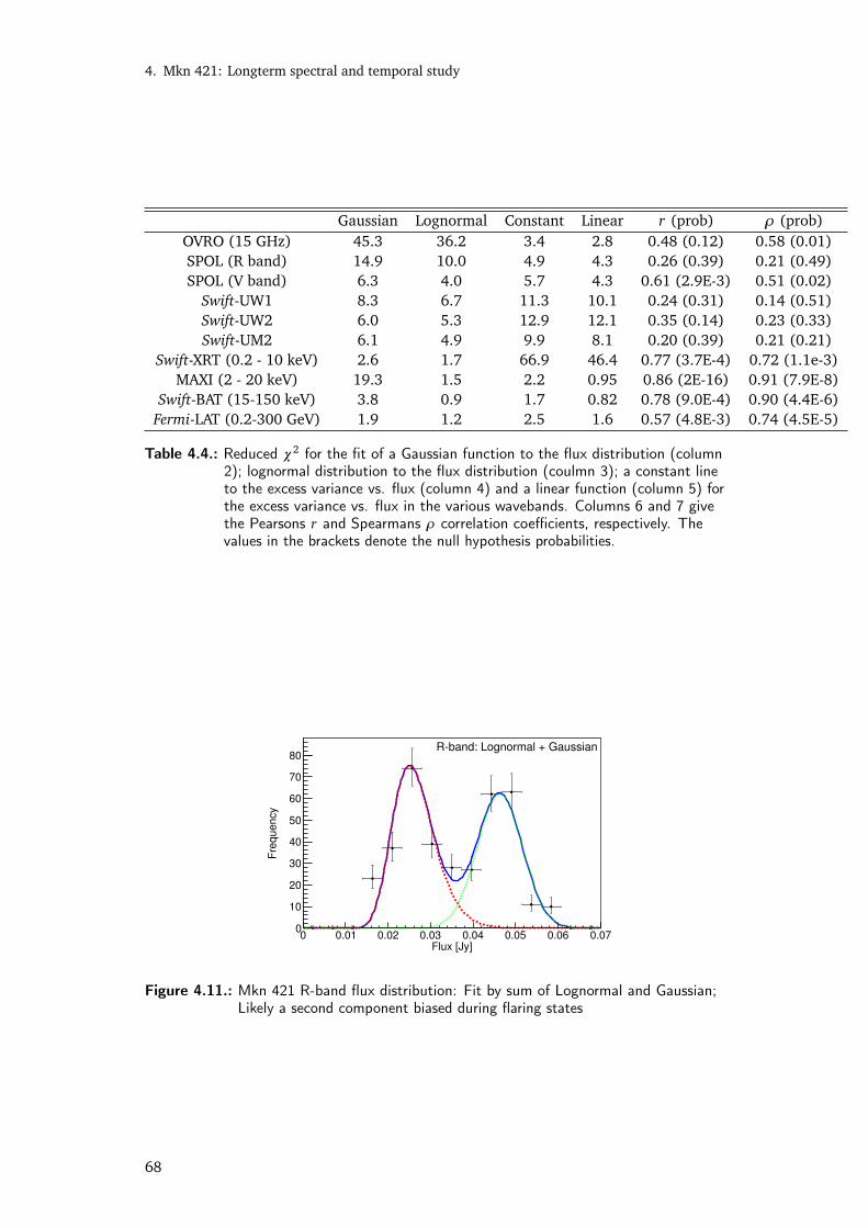
4. Mkn 421: Longterm spectral and temporal study
Gaussian Lognormal Constant Linear r (prob) ρ (prob)OVRO (15 GHz) 45.3 36.2 3.4 2.8 0.48 (0.12) 0.58 (0.01)SPOL (R band) 14.9 10.0 4.9 4.3 0.26 (0.39) 0.21 (0.49)SPOL (V band) 6.3 4.0 5.7 4.3 0.61 (2.9E-3) 0.51 (0.02)
Swift-UW1 8.3 6.7 11.3 10.1 0.24 (0.31) 0.14 (0.51)Swift-UW2 6.0 5.3 12.9 12.1 0.35 (0.14) 0.23 (0.33)Swift-UM2 6.1 4.9 9.9 8.1 0.20 (0.39) 0.21 (0.21)
Swift-XRT (0.2 - 10 keV) 2.6 1.7 66.9 46.4 0.77 (3.7E-4) 0.72 (1.1e-3)MAXI (2 - 20 keV) 19.3 1.5 2.2 0.95 0.86 (2E-16) 0.91 (7.9E-8)
Swift-BAT (15-150 keV) 3.8 0.9 1.7 0.82 0.78 (9.0E-4) 0.90 (4.4E-6)Fermi-LAT (0.2-300 GeV) 1.9 1.2 2.5 1.6 0.57 (4.8E-3) 0.74 (4.5E-5)
Table 4.4.: Reduced χ2 for the fit of a Gaussian function to the flux distribution (column2); lognormal distribution to the flux distribution (coulmn 3); a constant lineto the excess variance vs. flux (column 4) and a linear function (column 5) forthe excess variance vs. flux in the various wavebands. Columns 6 and 7 givethe Pearsons r and Spearmans ρ correlation coefficients, respectively. Thevalues in the brackets denote the null hypothesis probabilities.
Flux [Jy]0 0.01 0.02 0.03 0.04 0.05 0.06 0.07
Fre
qu
en
cy
0
10
20
30
40
50
60
70
80Rband: Lognormal + Gaussian
Figure 4.11.: Mkn 421 R-band flux distribution: Fit by sum of Lognormal and Gaussian;Likely a second component biased during flaring states
68

4.4. Spectral modelling
spherical zone of radius R filled with a tangled magnetic field B. A non-thermal population
of electrons, with a broken power-law spectral shape,
N(γ)dγ=
¨
Kγ−p1 dγ, γmin < γ < γb
Kγ(p2−p1)b γ−p2 dγ, γb < γ < γmax
(44)
is assumed to lose its energy through synchrotron and self-Compton (SSC) processes.
As a result of the relativistic motion of the jet, the radiation is boosted along our line
of sight by a Doppler factor δ. This simple model is most commonly used in literature
to model the broadband spectrum Ghisellini et al. (1996); Krawczynski et al. (2004).
Correction for attenuation of TeV photons due to the extragalactic background light
(EBL) is accounted for by deconvolving the obtained spectrum with the EBL model of
Franceschini et al. (2008). Mankuzhiyil et al. (2012) used the Levenburg-Marquadt
algorthim to fit the numerical model to the observed spectrum. We incorporate the
numerical SSC model of Saha & Bhattacharjee (2015) in the XSPEC spectral fitting
software to perform a χ2 minimization. More details about incorporating SSC model in
XSPEC can be found in Appendix A. Swift-XRT fluxes are averaged over ∼ 6 spectral bins
(and similarly for NuSTAR) to avoid biasing the fit towards the X-ray energies. The tool
flx2xsp v.2.1 was used to convert the fluxes to pha files for use in XSPEC. Since we
are dealing with several different instruments over a broad energy range, we assume
model systematics of 5%.
A good sampling of the entire SED from radio to γ-rays allows one to perform a
reasonable estimation of the physical parameters (Ghisellini et al., 1996; Tavecchio et al.,
1998) in terms of the observed fluxes. The radius R of the emission region has to be
independently estimated from the light travel time argument, R< cδtvar /(1+ z), where
tvar is the observed flux doubling timescale. However, Mkn 421 shows different flux
doubling timescales over different time periods, and since we are dealing mainly with
quiescent state emission, we keep R fixed at 6.0×1016 cm, which was used by Aleksic
et al. (2014a). This roughly corresponds to a tvar ∼ 1 day for δ = 21, which is also
frozen during the fitting. The minimum particle Lorentz factor, γmin can be fixed at a
reasonably low value without affecting the modelling (Cerruti, 2015a), and is assumed
to be 1000. The maximum Lorentz factor, γmax , is kept fixed at 10γb.
The ratio of the electric (UE) and magnetic (UB )field energy density is parame-
terized by the equipartition parameter η = UE/UB, where UB = B2/2µ0 and UE =
mec2γmax∫
γmin
γN(γ)dγ. The best fit SEDs are shown in Fig. 6.6, and the fit parameters and
the reduced χ2 listed in Table 4.5. During all the epochs, the energy density in the jet is
matter dominated with the model parameters a factor of 10 away from equipartition.
However, this ratio may be improved by choosing a lower value of δ or R. For all the
SEDs studied here, the one-zone model provides a very good fit to the observed data and
does not motivate the need for a second emitting region.
69
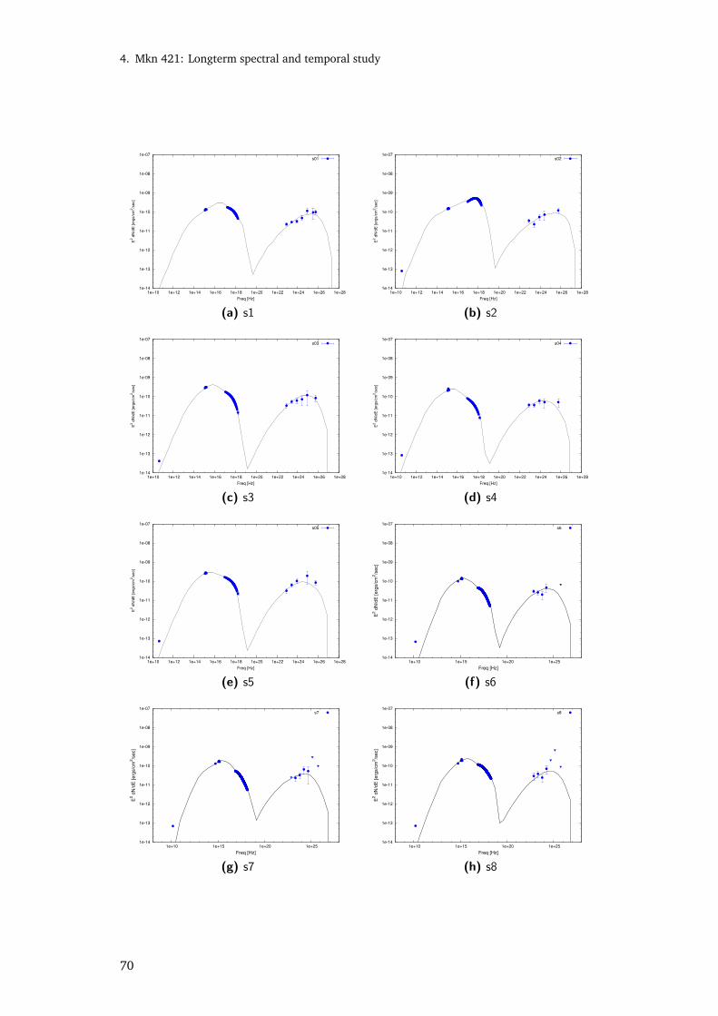
4. Mkn 421: Longterm spectral and temporal study
1e-14
1e-13
1e-12
1e-11
1e-10
1e-09
1e-08
1e-07
1e+10 1e+12 1e+14 1e+16 1e+18 1e+20 1e+22 1e+24 1e+26 1e+28
E2 d
N/d
E [
erg
s/c
m2/s
ec]
Freq [Hz]
s01
(a) s1
1e-14
1e-13
1e-12
1e-11
1e-10
1e-09
1e-08
1e-07
1e+10 1e+12 1e+14 1e+16 1e+18 1e+20 1e+22 1e+24 1e+26 1e+28
E2 d
N/d
E [
erg
s/c
m2/s
ec]
Freq [Hz]
s02
(b) s2
1e-14
1e-13
1e-12
1e-11
1e-10
1e-09
1e-08
1e-07
1e+10 1e+12 1e+14 1e+16 1e+18 1e+20 1e+22 1e+24 1e+26 1e+28
E2 d
N/d
E [
erg
s/c
m2/s
ec]
Freq [Hz]
s03
(c) s3
1e-14
1e-13
1e-12
1e-11
1e-10
1e-09
1e-08
1e-07
1e+10 1e+12 1e+14 1e+16 1e+18 1e+20 1e+22 1e+24 1e+26 1e+28
E2 d
N/d
E [
erg
s/c
m2/s
ec]
Freq [Hz]
s04
(d) s4
1e-14
1e-13
1e-12
1e-11
1e-10
1e-09
1e-08
1e-07
1e+10 1e+12 1e+14 1e+16 1e+18 1e+20 1e+22 1e+24 1e+26 1e+28
E2 d
N/d
E [
erg
s/c
m2/s
ec]
Freq [Hz]
s05
(e) s5
1e-14
1e-13
1e-12
1e-11
1e-10
1e-09
1e-08
1e-07
1e+10 1e+15 1e+20 1e+25
E2 d
N/d
E [erg
s/c
m2/s
ec]
Freq [Hz]
s6
(f) s6
1e-14
1e-13
1e-12
1e-11
1e-10
1e-09
1e-08
1e-07
1e+10 1e+15 1e+20 1e+25
E2 d
N/d
E [erg
s/c
m2/s
ec]
Freq [Hz]
s7
(g) s7
1e-14
1e-13
1e-12
1e-11
1e-10
1e-09
1e-08
1e-07
1e+10 1e+15 1e+20 1e+25
E2 d
N/d
E [erg
s/c
m2/s
ec]
Freq [Hz]
s8
(h) s8
70

4.4. Spectral modelling
1e-14
1e-13
1e-12
1e-11
1e-10
1e-09
1e-08
1e-07
1e+10 1e+15 1e+20 1e+25
E2 d
N/d
E [erg
s/c
m2/s
ec]
Freq [Hz]
s9
(a) s9
1e-14
1e-13
1e-12
1e-11
1e-10
1e-09
1e-08
1e-07
1e+10 1e+15 1e+20 1e+25
E2 d
N/d
E [erg
s/c
m2/s
ec]
Freq [Hz]
s10
(b) s10
1e-14
1e-13
1e-12
1e-11
1e-10
1e-09
1e-08
1e-07
1e+10 1e+15 1e+20 1e+25
E2 d
N/d
E [erg
s/c
m2/s
ec]
Freq [Hz]
s11
(c) s11
1e-14
1e-13
1e-12
1e-11
1e-10
1e-09
1e-08
1e-07
1e+10 1e+15 1e+20 1e+25
E2 d
N/d
E [erg
s/c
m2/s
ec]
Freq [Hz]
s12
(d) s12
1e-14
1e-13
1e-12
1e-11
1e-10
1e-09
1e-08
1e-07
1e+10 1e+15 1e+20 1e+25
E2 d
N/d
E [erg
s/c
m2/s
ec]
Freq [Hz]
s13
(e) s13
1e-14
1e-13
1e-12
1e-11
1e-10
1e-09
1e-08
1e-07
1e+10 1e+15 1e+20 1e+25
E2 d
N/d
E [erg
s/c
m2/s
ec]
Freq [Hz]
s14
(f) s14
1e-14
1e-13
1e-12
1e-11
1e-10
1e-09
1e-08
1e-07
1e+10 1e+15 1e+20 1e+25
E2 d
N/d
E [erg
s/c
m2/s
ec]
Freq [Hz]
s15
(g) s15
1e-14
1e-13
1e-12
1e-11
1e-10
1e-09
1e-08
1e-07
1e+10 1e+15 1e+20 1e+25
E2 d
N/d
E [erg
s/c
m2/s
ec]
Freq [Hz]
s16
(h) s16
71
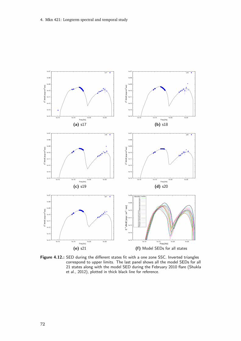
4. Mkn 421: Longterm spectral and temporal study
1e-14
1e-13
1e-12
1e-11
1e-10
1e-09
1e-08
1e-07
1e+10 1e+15 1e+20 1e+25
E2 d
N/d
E [erg
s/c
m2/s
ec]
Freq [Hz]
s17
(a) s17
1e-14
1e-13
1e-12
1e-11
1e-10
1e-09
1e-08
1e-07
1e+10 1e+15 1e+20 1e+25
E2 d
N/d
E [erg
s/c
m2/s
ec]
Freq [Hz]
s18
(b) s18
1e-14
1e-13
1e-12
1e-11
1e-10
1e-09
1e-08
1e-07
1e+10 1e+15 1e+20 1e+25
E2 d
N/d
E [erg
s/c
m2/s
ec]
Freq [Hz]
s19
(c) s19
1e-14
1e-13
1e-12
1e-11
1e-10
1e-09
1e-08
1e-07
1e+10 1e+15 1e+20 1e+25
E2 d
N/d
E [erg
s/c
m2/s
ec]
Freq [Hz]
s20
(d) s20
1e-14
1e-13
1e-12
1e-11
1e-10
1e-09
1e-08
1e-07
1e+10 1e+15 1e+20 1e+25
E2 d
N/d
E [erg
s/c
m2/s
ec]
Freq [Hz]
s21
(e) s21
1e-14
1e-13
1e-12
1e-11
1e-10
1e-09
1e-08
1e+10 1e+15 1e+20 1e+25
E 2
dN
/dE
[erg
s / c
m2 / s
ec]
Freq [Hz]
Feb 2010s1s2s3s4s5s6s7s8s9
s10s11s12s13s14s15s16s17s18s19s20s21
(f) Model SEDs for all states
Figure 4.12.: SED during the different states fit with a one zone SSC. Inverted trianglescorrespond to upper limits. The last panel shows all the model SEDs for all21 states along with the model SED during the February 2010 flare (Shuklaet al., 2012), plotted in thick black line for reference.
72

4.5. Results and discussions
p1 p2 ln(γb) B(G) UE(ergs/cc) η= UE/UB L (ergs/sec) χ2
s1 2.2 4.0 11.79 2.94E-02 4.53E-04 13.1 4.86E+45 1.65s2 2.4 4.8 13.15 3.79E-02 4.47E-04 7.79 8.28E+45 0.98s3 1.8 3.7 10.62 4.22E-02 4.33E-04 6.12 6.41E+45 0.48s4 2.0 3.8 10.38 3.99E-02 4.50E-04 7.10 4.00E+45 0.46s5 1.7 3.3 10.03 3.97E-02 4.84E-04 7.70 5.45E+45 0.51s6 2.1 3.8 10.37 2.91E-02 5.08E-04 15.0 2.44E+45 1.26s7 2.2 4.1 10.52 3.99E-02 4.85E-04 7.65 3.06E+45 0.90s8 1.9 3.6 10.41 4.13E-02 3.82E-04 5.63 4.01E+45 1.38s9 2.4 3.8 11.30 4.42E-02 5.56E-04 7.16 5.80E+45 0.90
s10 2.1 4.4 11.24 4.59E-02 4.48E-04 5.34 7.45E+45 1.30s11 1.6 4.2 10.52 3.05E-02 5.06E-04 13.6 3.84E+45 2.35s12 2.8 4.5 12.13 3.91E-02 6.29E-04 10.3 8.69E+45 1.90s13 2.7 4.8 13.15 3.85E-02 6.35E-04 10.7 1.50E+46 1.52s14 2.3 4.0 11.14 4.42E-02 4.90E-04 6.29 8.32E+45 1.43s15 2.5 3.9 12.73 3.65E-02 4.99E-04 9.40 8.03E+45 1.32s16 1.9 3.9 11.13 4.38E-02 3.65E-04 4.77 6.20E+45 1.34s17 2.6 4.3 12.39 3.57E-02 7.05E-04 13.8 7.02E+45 0.97s18 2.3 3.7 11.88 2.99E-02 8.22E-04 23.1 9.32E+45 1.01s19 2.2 3.1 11.68 3.53E-02 5.31E-04 10.7 8.01E+45 1.98s20 2.3 3.0 12.23 2.71E-02 8.06E-04 27.5 8.42E+45 1.10s21 2.3 3.4 12.17 3.58E-02 6.28E-04 12.3 9.40E+45 1.59
Table 4.5.: Fit parameters for the different SED states with R = 6.0× 1016 cm, δ = 21,γmin = 1000, and γmax = 10γb
4.5 R E S U LT S A N D D I S C U S S I O N S
4.5.1 Spectral variability
The similar variability in the optical-GeV bands, and the X-ray-VHE bands indicates a
similar origin for the optical and Fermi-LAT bands and for the X-ray-VHE bands. In the
framework of the SSC model, this is attributed as the first index, p1 contributing to the
optical-GeV bands (synchrotron and SSC respectively), and the second index p2 for the
X-ray-VHE bands. As can be seen from the fit parameters in Table 4.5, some of the states
require a very hard particle index p1 < 2.0. Such an index cannot originate from a single
shock acceleration, but may originate from multiple shocks Malkov & Drury (2001),
which can produce particle indices as hard as 1.5, which is close to the hardest spectrum
(p1 = 1.6) obtained in our fits. Alternatively, stochastic acceleration in resonance with
plasma wave turbulence behind the relativistic shock front can also harden the injection
index (Vainio et al., 2004). The two indices, p1 and p2, show a weak correlation with
ρ = 0.42, prob = 0.05 (Figure 4.13a). In particular, p2 is much steeper than what
would be expected from p2 = p1 + 1, thus ruling out the broken power-law spectrum
as originating from a cooling break. There is a significant correlation between the total
bolometric luminosity L and the first index (ρ = 0.66, prob = 0.001), and a very strong
correlation between L and the particle break energy γb (ρ = 0.79, prob = 3.2×10⁻⁵)
(Fig 4.13b). However, no significant trend is seen between the magnetic field B and L.
73
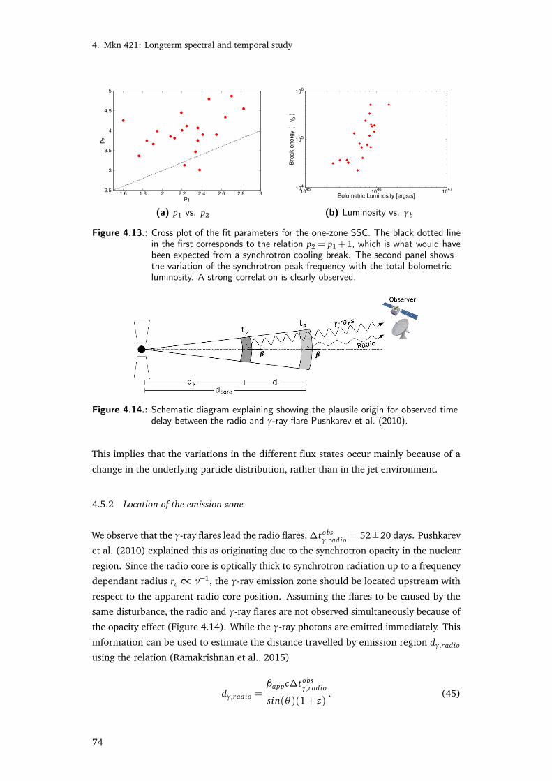
4. Mkn 421: Longterm spectral and temporal study
2.5
3
3.5
4
4.5
5
1.6 1.8 2 2.2 2.4 2.6 2.8 3
p2
p1
(a) p1 vs. p2
104
105
106
1045
1046
1047
Bre
ak e
nerg
y (
γ
b )
Bolometric Luminosity [ergs/s]
(b) Luminosity vs. γb
Figure 4.13.: Cross plot of the fit parameters for the one-zone SSC. The black dotted linein the first corresponds to the relation p2 = p1 + 1, which is what would havebeen expected from a synchrotron cooling break. The second panel showsthe variation of the synchrotron peak frequency with the total bolometricluminosity. A strong correlation is clearly observed.
Figure 4.14.: Schematic diagram explaining showing the plausile origin for observed timedelay between the radio and γ-ray flare Pushkarev et al. (2010).
This implies that the variations in the different flux states occur mainly because of a
change in the underlying particle distribution, rather than in the jet environment.
4.5.2 Location of the emission zone
We observe that the γ-ray flares lead the radio flares,∆tobsγ,radio = 52±20 days. Pushkarev
et al. (2010) explained this as originating due to the synchrotron opacity in the nuclear
region. Since the radio core is optically thick to synchrotron radiation up to a frequency
dependant radius rc ∝ ν−1, the γ-ray emission zone should be located upstream with
respect to the apparent radio core position. Assuming the flares to be caused by the
same disturbance, the radio and γ-ray flares are not observed simultaneously because of
the opacity effect (Figure 4.14). While the γ-ray photons are emitted immediately. This
information can be used to estimate the distance travelled by emission region dγ,radio
using the relation (Ramakrishnan et al., 2015)
dγ,radio =βappc∆tobs
γ,radio
sin(θ )(1+ z). (45)
74
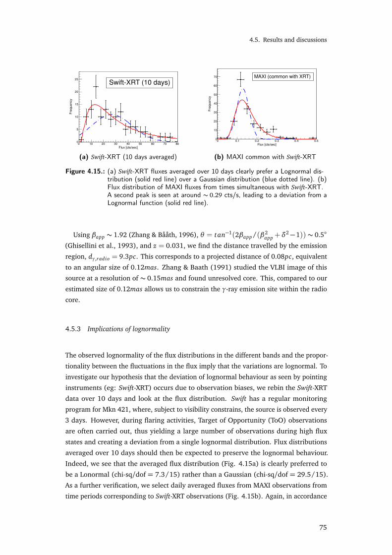
4.5. Results and discussions
Flux [cts/sec]0 10 20 30 40 50 60 70 80
Fre
qu
en
cy
0
5
10
15
20
25
SwiftXRT (10 days)
(a) Swift-XRT (10 days averaged)
Flux [cts/sec]0 0.1 0.2 0.3 0.4 0.5
Fre
qu
en
cy
0
10
20
30
40
50
60
70 MAXI (common with XRT)
(b) MAXI common with Swift-XRT
Figure 4.15.: (a) Swift-XRT fluxes averaged over 10 days clearly prefer a Lognormal dis-tribution (solid red line) over a Gaussian distribution (blue dotted line). (b)Flux distribution of MAXI fluxes from times simultaneous with Swift-XRT.A second peak is seen at around ∼ 0.29 cts/s, leading to a deviation from aLognormal function (solid red line).
Using βapp ∼ 1.92 (Zhang & Bååth, 1996), θ = tan−1(2βapp/(β2app +δ
2−1)) ∼ 0.5
(Ghisellini et al., 1993), and z = 0.031, we find the distance travelled by the emission
region, dγ,radio = 9.3pc. This corresponds to a projected distance of 0.08pc, equivalent
to an angular size of 0.12mas. Zhang & Baath (1991) studied the VLBI image of this
source at a resolution of ∼ 0.15mas and found unresolved core. This, compared to our
estimated size of 0.12mas allows us to constrain the γ-ray emission site within the radio
core.
4.5.3 Implications of lognormality
The observed lognormality of the flux distributions in the different bands and the propor-
tionality between the fluctuations in the flux imply that the variations are lognormal. To
investigate our hypothesis that the deviation of lognormal behaviour as seen by pointing
instruments (eg: Swift-XRT) occurs due to observation biases, we rebin the Swift-XRT
data over 10 days and look at the flux distribution. Swift has a regular monitoring
program for Mkn 421, where, subject to visibility constrains, the source is observed every
3 days. However, during flaring activities, Target of Opportunity (ToO) observations
are often carried out, thus yielding a large number of observations during high flux
states and creating a deviation from a single lognormal distribution. Flux distributions
averaged over 10 days should then be expected to preserve the lognormal behaviour.
Indeed, we see that the averaged flux distribution (Fig. 4.15a) is clearly preferred to
be a Lonormal (chi-sq/dof = 7.3/15) rather than a Gaussian (chi-sq/dof = 29.5/15).
As a further verification, we select daily averaged fluxes from MAXI observations from
time periods corresponding to Swift-XRT observations (Fig. 4.15b). Again, in accordance
75
4. Mkn 421: Longterm spectral and temporal study
with our conjecture, we see a deviation from a Lognormal distribution (chi-sq/dof =
21.9/10).
Similar lognormal trends have been found in several accreting galactic sources (Giebels
& Degrange, 2009) and also in the Seyfert 1 galaxy, Mkn 766, where the physical process
responsible for the X-ray emission is most likely thermal emission from the galactic
disk (Vaughan et al., 2003). The results of our SED modelling in Section 5.4 show that
the flux variability in the source can be mainly attributed to changes in the particle
spectrum rather than jet parameters such as the magnetic field or Doppler factor. This
implies that the lognormal fluctuations in the flux are indicative of lognormal processes
in the accretion disk, and the lognormal fluctuations in the accreting rate give rise to an
injection rate with similar properties.
4.6 C O N C LU S I O N S
In this chapter, we have presented a 7-year continuous multi-wavelength monitoring
of Mkn 421, from March 2009 to April 2015, a period that includes both steady states
and episodes of strong flaring activity. The variability increases with energy for both
the SED components, thus supporting a SSC emission mechanism. This idea is further
supported by the observed optical-GeV and the known X-ray TeV (Bartoli et al., 2015)
correlations. A simple one zone model incorporating synchrotron and SSC mechanisms
provided a suitable fit to the observed SEDs for all epochs without motivating the need for
any additional emitting regions. Interestingly, while the time-resolved UV-X-ray spectra
during the April 2013 flare could not be explained by synchrotron emission from a single
region (Sinha et al., 2015), the time averaged broadband spectrum during the same time
(State s13) can be well fitted by our model (Reduced χ2 = 1.5). This motivates a need
for better time-resolved broadband spectra. The detection of lognormal flux behaviour
in a blazar also encourages us to take a new look into our understanding of jet lauching
mechanisms in supermassive black holes. A long term continuous monitoring program
for a set of blazars may turn out very profitable in this regard. The upcoming Major
Atmospheric Cherenkov Experiment (MACE; Koul et al. (2011)) at Hanle, Ladakh is
expected to provide us with excellent time-resolved spectrum at VHE energies, which
may throw new light onto the VHE emission from blazar jets.
76
“To confine our attention to terrestrial matters would be to
limit the human spirit."
Stephen Hawking
5Mkn 421: Underlying particlespectrum during giant flare
DURING APRIL 2013, MKN 421 underwent one of the largest flares in X-rays in the past
decade, and was the subject of an intense multiwavelength campaign with both space and
ground based observational facilities. The dramatic flare allowed us an unprecendented
glimpse into a typical blackhole jet - undelying particle distributions (Sinha et al., 2015),
peculiar variability patterns (Paliya et al., 2015a), multicomponent, multizone emission
states Pian et al. (2014), etc. In this chapter we use multiwavelength data available
during MJD 56392 to 56403, with special emphasis on X-ray data using the Swift and
NuSTAR telescopes, to understand the underlying particle energy distribution.
5.1 B E H AV I O U R D U R I N G P R E V I O U S F L A R E S
Being one of the brightest and most variable source in the extragalactic sky, Mkn 421
has been extensively studied during its high activity states by several authors(Aleksic
et al., 2012b; Shukla et al., 2012; Isobe et al., 2010; Krawczynski et al., 2001; Aleksic
et al., 2010; Acciari et al., 2009d; Ushio et al., 2009; Tramacere et al., 2009; Horan
et al., 2009; Lichti et al., 2008; Fossati et al., 2008; Albert et al., 2007a; Brinkmann
et al., 2003; Singh et al., 2015), a detailed review of which is beyond the scope of this
thesis. Its optical brightness was found to change by 1.4 mag in 2.5 hrs during a flare in
1986 (Guangzhong et al., 1988). A very fast flux doubling time of 14.01±5.03 minutes,
which is on the order of the light crossing time of the black hole’s event horizon, has
been seen at hard X-rays using NuSTAR data during the rapid flare in April 2013 (Paliya
et al., 2015a). Since its detection, the source has been generally very active in the high
energy bands, with a big eruption on a timescale of ∼ 2 years (Bartoli et al., 2015; Cui,
77
5. Mkn 421: Underlying particle spectrum during giant flare
2004; Gaur et al., 2012; Tluczykont et al., 2010). A major outburst is generally seen
to be followed by several smaller flares. Gaidos et al. (1996) detected extremely fast
VHE outbursts were where the doubling time of the flare events were found to be < 15
minutes. The X-ray emission is known to be highly correlated with the TeV emission
(Błazejowski et al., 2005; K. Katarzynski et al., 2005; jie Qian et al., 1998), but like other
HBLs, shows moderate correlation with the GeV emission (Li et al., 2013).
In the spring-summer 2006, Tramacere et al. (2009) found that the X-ray flux of Mrk
421 reached its highest record till date. In 2006 April, Mrk 421 underwent a large flare
and the X-ray flux was variable (Ushio et al., 2010). In 2010 January and February, big
X-ray outbursts were observed from the object Isobe et al. (2010); Shukla et al. (2012).
X-ray and TeV outbursts were also reported for the source by Kerrick et al. (1995) and
Takahashi et al. (1994, 1995) in 1994 and 1995, respectively.
5.2 M U LT I WAV E L E N GT H O B S E RVAT I O N S A N D DATA A N A LY S I S
The huge X-ray flare of Mkn 421 in April 2013 (2013 April 10 to 21; MJD 56392−56403)
was simultaneously observed by the NuSTAR and Swift X-ray and UV telescopes. There
were 11 NuSTAR pointings and 15 Swift pointings within the dates of interest, the details
of which are given in Table 5.1 and Table 5.2 respectively. Data are processed according to
the standard procedures outlined in Chapter 3.2 and Chapter 3.3. To achieve strict simul-
taneity with Swift-XRT observations, NuSTAR observation id 60002023025 is broken into
four parts: 56393.15591890 to 56393.29538714, 56393.29538714 to 56393.91093765,
56393.91093765 to 56393.96788711, and 56393.96788711 to 56394.37822500 MJD.
Swift-UVOT (Roming et al., 2005) operated in imaging mode during this period, and
for most of the observations, cycled through the UV filters UW1, UW2, and UM2. The
tool uvotsource v.3.3 is used to extract the fluxes from each of the images using
aperture photometry. The observed magnitudes were corrected for Galactic extinction
(EB−V = 0.019 mag) using the dust maps of Schlegel et al. (1998) and converted to flux
units using the zero-point magnitudes and conversion factors of Breeveld et al. (2011).
The tool flx2xsp v.2.1 is used to convert the fluxes to pha files for use in XSPEC.
The γ-ray behaviour of this source during this flare is obtained by collecting Fermi-LAT
observations covering the period of the X-ray outburst (MJD 56390−56403), analysed
according to the procedure described in Chapter 3.1. A simple power law spectral model,
with index and normalisation as the free parameters, is used to model the source.
In addition, we also include the X-ray observations by the Swift-BAT and the MAXI
telescopes and optical observations by SPOL-CCD. Significant flux brightening at TeV
energies is seen with the HAGAR array of Telescopes. Source brightened from the level
of 1 Crab unit to about 3 Crab units from March to April observation season Acharya
et al. (2013), simultaneous with the X-ray flare (Figure 5.1). Unfortunately, many nights
were lost due to poor sky conditions, and detailed analysis could not be carried out.
78
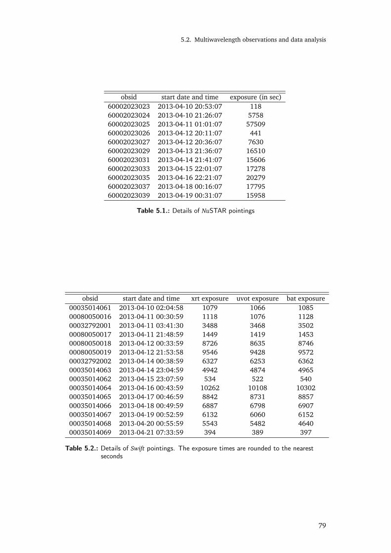
5.2. Multiwavelength observations and data analysis
obsid start date and time exposure (in sec)60002023023 2013-04-10 20:53:07 11860002023024 2013-04-10 21:26:07 575860002023025 2013-04-11 01:01:07 5750960002023026 2013-04-12 20:11:07 44160002023027 2013-04-12 20:36:07 763060002023029 2013-04-13 21:36:07 1651060002023031 2013-04-14 21:41:07 1560660002023033 2013-04-15 22:01:07 1727860002023035 2013-04-16 22:21:07 2027960002023037 2013-04-18 00:16:07 1779560002023039 2013-04-19 00:31:07 15958
Table 5.1.: Details of NuSTAR pointings
obsid start date and time xrt exposure uvot exposure bat exposure00035014061 2013-04-10 02:04:58 1079 1066 108500080050016 2013-04-11 00:30:59 1118 1076 112800032792001 2013-04-11 03:41:30 3488 3468 350200080050017 2013-04-11 21:48:59 1449 1419 145300080050018 2013-04-12 00:33:59 8726 8635 874600080050019 2013-04-12 21:53:58 9546 9428 957200032792002 2013-04-14 00:38:59 6327 6253 636200035014063 2013-04-14 23:04:59 4942 4874 496500035014062 2013-04-15 23:07:59 534 522 54000035014064 2013-04-16 00:43:59 10262 10108 1030200035014065 2013-04-17 00:46:59 8842 8731 885700035014066 2013-04-18 00:49:59 6887 6798 690700035014067 2013-04-19 00:52:59 6132 6060 615200035014068 2013-04-20 00:55:59 5543 5482 464000035014069 2013-04-21 07:33:59 394 389 397
Table 5.2.: Details of Swift pointings. The exposure times are rounded to the nearestseconds
79
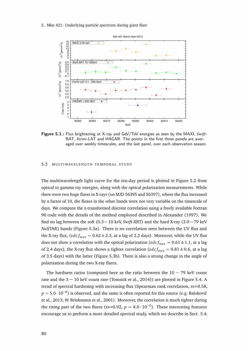
5. Mkn 421: Underlying particle spectrum during giant flare
2 4 6 8
10 12 14 16
10
-2 [
ph
/cm
2/s
]
Mrk-421 March-April 2013
MAXI 2-20 keV
-0.1 0
0.1 0.2 0.3 0.4 0.5
10
-2 [
ph
/cm
2/s
]
Swift-BAT 15-150keV
2.5
3.5
4.5
5.5
6.5
7.5
10
-7 [
ph
/cm
2/s
]
Fermi-LAT 0.1 - 300 GeV
-1 0 1 2 3 4
56350 56360 56370 56380 56390 56400 56410 56420
Cra
b U
nits
MJD
HAGAR > 250 GeV
Figure 5.1.: Flux brightening at X-ray and GeV/TeV energies as seen by the MAXI, Swift-BAT, Fermi-LAT and HAGAR. The points in the first three panels are aver-aged over weekly timescales, and the last panel, over each observation season.
5.3 M U LT I WAV E L E N GT H T E M P O R A L S T U DY
The multiwavelength light curve for the ten-day period is plotted in Figure 5.2 from
optical to gamma ray energies, along with the optical polarization measurements. While
there were two huge flares in X-rays (on MJD 56395 and 56397), where the flux increased
by a factor of 10, the fluxes in the other bands were not very variable on the timescale of
days. We compute the z-transformed discrete correlation using a freely available Fortran
90 code with the details of the method employed described in Alexander (1997). We
find no lag between the soft (0.3−10 keV, Swift-XRT) and the hard X-ray (3.0−79 keV
NuSTAR) bands (Figure 5.3a). There is no correlation seen between the UV flux and
the X-ray flux, (zdc fmax = 0.62±2.3, at a lag of 2.2 days). Moreover, while the UV flux
does not show a correlation with the optical polarization (zdc fmax = 0.61±1.1, at a lag
of 2.4 days), the X-ray flux shows a tighter correlation (zdc fmax = 0.81±0.6, at a lag
of 3.5 days) with the latter (Figure 5.3b). There is also a strong change in the angle of
polarization during the two X-ray flares.
The hardness ratios (computed here as the ratio between the 10 − 79 keV count
rate and the 3 − 10 keV count rate (Tomsick et al., 2014)) are plotted in Figure 5.4. A
trend of spectral hardening with increasing flux (Spearman rank correlation, rs=0.58,
p = 5.0 ·10−8) is observed, and the same is often reported for this source (e.g. Balokovic
et al., 2013; W. Brinkmann et al., 2001). Moreover, the correlation is much tighter during
the rising part of the two flares (rs=0.92, p = 4.0 · 10−5). These interesting features
encourage us to perform a more detailed spectral study, which we describe in Sect. 5.4.
80
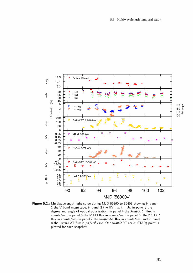
5.3. Multiwavelength temporal study
11.9
12.1
12.3
mag
Optical V band
15 20 25 30
mJy
UM2
UW2
UW1
1
3
5
100
130
160
190
Pola
rization [%
]
Pol angle
pol deg
pol ang
0
80
160
240
cts
/s
Swift-XRT 0.2-10 keV
-0.05 0.05 0.15 0.25
cts
/s
MAXI 2-20 keV
0
20
40
60
cts
/s
NuStar 3-79 keV
-0.005 0
0.005 0.01
cts
/s
Swift-BAT 15-50 keV
0.5 1.5 2.5 3.5 4.5
90 92 94 96 98 100 102
ph 1
0^7
MJD [56300+]
LAT 0.2-300GeV
Figure 5.2.: Multiwavelength light curve during MJD 56390 to 56403 showing in panel1 the V-band magnitude, in panel 2 the UV flux in mJy, in panel 3 thedegree and angle of optical polarization, in panel 4 the Swift-XRT flux incounts/sec, in panel 5 the MAXI flux in counts/sec, in panel 6: theNuSTARflux in counts/sec, in panel 7 the Swift-BAT flux in counts/sec, and in panel8 the Fermi-LAT flux in ph/cm2/sec. One Swift-XRT (or NuSTAR) point isplotted for each snapshot.
81

5. Mkn 421: Underlying particle spectrum during giant flare
Energy band Frms Number of obs.V band 0.08±0.01 28um2 0.10±0.001 58uw2 0.08±0.002 60uw1 0.09±0.0.001 62maxi 0.717±0.009 11xrt 0.726±0.002 59bat 0.854±0.019 11
nustar 0.752±0.001 85fermi 0.16±0.07 10
Table 5.3.: The Frms for each energy band between MJD 56390 to 56400.
The fractional variability amplitude parameter Fvar (Chapter 4.3.1, computed on
daily timescales, is used to quantify the multiwavelength variability. The variability
amplitude at the different wavelengths is tabulated in Table 5.3, and is found to be
the highest for the X-ray bands (Fvar ∼ 0.75± 0.10) and significantly lower for the
UV bands (Fvar ∼ 0.08±0.02), suggesting that the emission may probably arise from
different components in the two bands. The variability in the GeV range is also weak
(Fvar ∼ 0.16± 0.07). This contradicts the general trend found in blazars that Fvar is
highest for the γ-ray band and decreases with frequency (Zhang et al., 2005; Paliya et al.,
2015b). Moreover, there is an indication of a TeV flare with rapid flux variations during
this time (Cortina & Holder, 2013; Pian et al., 2014).
We scan the Swift-XRT and the NuSTAR light curves for the shortest flux-doubling
timescale using the following equation (Foschini et al., 2011):
F(t) = F(t0).2(t−t0)/τ, (46)
where F(t) and F(t0) are the fluxes at time t and t0 , respectively, and τ is the
characteristic doubling or halving timescale. The fastest observed variability in the
NuSTAR band is 1.69±0.08 hours between MJD 97.06438 to 97.08573. This is similar to
the very fast variability observed in this source with the Beppo-SAX (Fossati et al., 2000).
This study was only performed for those periods where the flux difference was signifi-
cant, at least at the 3σ level.
5.4 X-R AY S P E C T R A L A N A LY S I S
The close simultaneity between Swift-XRT and NuSTAR observations allows us to perform
a joint spectral fitting using XSPEC package v.12.8.2. The time periods that are
fitted together are shown in Figure 5.5. The bin widths were selected as one bin per
Swift-XRT observation (except for Obs. id. 00035014062 and 00035014069, which
lasted only for a few minutes), leading to 13 time bins that we denote as f1 - f13. The
82
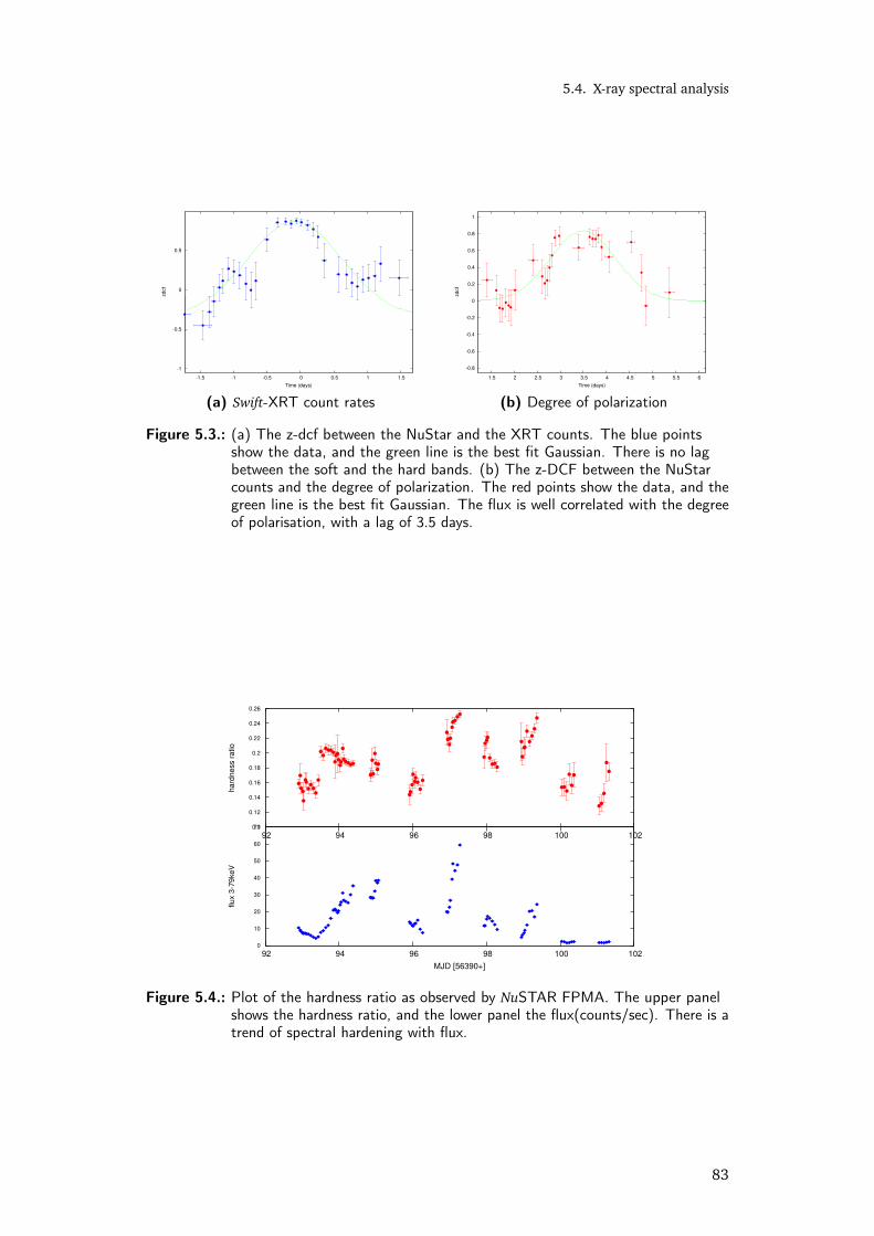
5.4. X-ray spectral analysis
-1
-0.5
0
0.5
-1.5 -1 -0.5 0 0.5 1 1.5
zdcf
Time (days)
(a) Swift-XRT count rates
-0.8
-0.6
-0.4
-0.2
0
0.2
0.4
0.6
0.8
1
1.5 2 2.5 3 3.5 4 4.5 5 5.5 6
zdcf
Time (days)
(b) Degree of polarization
Figure 5.3.: (a) The z-dcf between the NuStar and the XRT counts. The blue pointsshow the data, and the green line is the best fit Gaussian. There is no lagbetween the soft and the hard bands. (b) The z-DCF between the NuStarcounts and the degree of polarization. The red points show the data, and thegreen line is the best fit Gaussian. The flux is well correlated with the degreeof polarisation, with a lag of 3.5 days.
0.1
0.12
0.14
0.16
0.18
0.2
0.22
0.24
0.26
92 94 96 98 100 102
ha
rdn
ess r
atio
0
10
20
30
40
50
60
70
92 94 96 98 100 102
flu
x 3
-79
ke
V
MJD [56390+]
Figure 5.4.: Plot of the hardness ratio as observed by NuSTAR FPMA. The upper panelshows the hardness ratio, and the lower panel the flux(counts/sec). There is atrend of spectral hardening with flux.
83

5. Mkn 421: Underlying particle spectrum during giant flare
0
20
40
60
80
100
120
140
160
180
200
220
240
92 94 96 98 100 102 104 0
10
20
30
40
50
60
XR
T c
ounts
Nusta
r counts
MJD [ 56300+ ]
1 2 3 4 5 6 7 8 9 10 11 12 13
XRT
NuStar
Figure 5.5.: Thirteen time bins for which spectra have been extracted.
state f3 has no Swift-XRT data, whereas the state f13 has no NuSTAR data. Again in
Table 5.4 we list the Swift-XRT and corresponding NuSTAR data that were combined.
While fitting the broadband X-ray spectrum (0.3−79 keV), the XRT and the NuSTAR
spectral parameters are tied to each other, except for the relative normalization between
the two instruments. To correct for the line-of-sight absorption of soft X-rays due to the
interstellar gas, the neutral hydrogen column density is fixed at NH = 1.92×1020cm−2
(Kalberla et al., 2005).
5.4.1 Fitting the photon spectrum
It is known that the X-ray spectrum of Mkn 421 shows significant curvature (Fossati
et al., 2000; Massaro et al., 2004), and consistently, we also note that the data cannot
be fitted satisfactorily by a simple power law. On the other hand, a power law with an
exponential cutoff gives a much steeper curvature than observed, yielding unacceptable
fits. A sharp broken power-law also gives high χ2 values in most cases, which suggests a
smooth intrinsic curvature in the spectrum. Following (Massaro et al., 2004; Tramacere
et al., 2007), we therefore fitted the observed spectrum with a log parabola given by
dN/dE = K(E/Eb)−αs−βs log(E/Eb,s), (47)
where αs gives the spectral index at Eb,s. The point of maximum curvature, Ep,s is given
by
Ep,s = Eb,s10(2−αs)/2βs . (48)
84
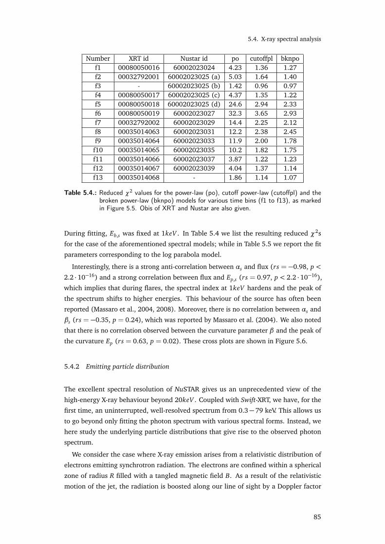
5.4. X-ray spectral analysis
Number XRT id Nustar id po cutoffpl bknpof1 00080050016 60002023024 4.23 1.36 1.27f2 00032792001 60002023025 (a) 5.03 1.64 1.40f3 - 60002023025 (b) 1.42 0.96 0.97f4 00080050017 60002023025 (c) 4.37 1.35 1.22f5 00080050018 60002023025 (d) 24.6 2.94 2.33f6 00080050019 60002023027 32.3 3.65 2.93f7 00032792002 60002023029 14.4 2.25 2.12f8 00035014063 60002023031 12.2 2.38 2.45f9 00035014064 60002023033 11.9 2.00 1.78
f10 00035014065 60002023035 10.2 1.82 1.75f11 00035014066 60002023037 3.87 1.22 1.23f12 00035014067 60002023039 4.04 1.37 1.14f13 00035014068 - 1.86 1.14 1.07
Table 5.4.: Reduced χ2 values for the power-law (po), cutoff power-law (cutoffpl) and thebroken power-law (bknpo) models for various time bins (f1 to f13), as markedin Figure 5.5. Obis of XRT and Nustar are also given.
During fitting, Eb,s was fixed at 1keV . In Table 5.4 we list the resulting reduced χ2s
for the case of the aforementioned spectral models; while in Table 5.5 we report the fit
parameters corresponding to the log parabola model.
Interestingly, there is a strong anti-correlation between αs and flux (rs = −0.98, p <
2.2 ·10−16) and a strong correlation between flux and Ep,s (rs = 0.97, p < 2.2 ·10−16),
which implies that during flares, the spectral index at 1keV hardens and the peak of
the spectrum shifts to higher energies. This behaviour of the source has often been
reported (Massaro et al., 2004, 2008). Moreover, there is no correlation between αs and
βs (rs = −0.35, p = 0.24), which was reported by Massaro et al. (2004). We also noted
that there is no correlation observed between the curvature parameter β and the peak of
the curvature Ep (rs = 0.63, p = 0.02). These cross plots are shown in Figure 5.6.
5.4.2 Emitting particle distribution
The excellent spectral resolution of NuSTAR gives us an unprecedented view of the
high-energy X-ray behaviour beyond 20keV . Coupled with Swift-XRT, we have, for the
first time, an uninterrupted, well-resolved spectrum from 0.3−79 keV. This allows us
to go beyond only fitting the photon spectrum with various spectral forms. Instead, we
here study the underlying particle distributions that give rise to the observed photon
spectrum.
We consider the case where X-ray emission arises from a relativistic distribution of
electrons emitting synchrotron radiation. The electrons are confined within a spherical
zone of radius R filled with a tangled magnetic field B. As a result of the relativistic
motion of the jet, the radiation is boosted along our line of sight by a Doppler factor
85
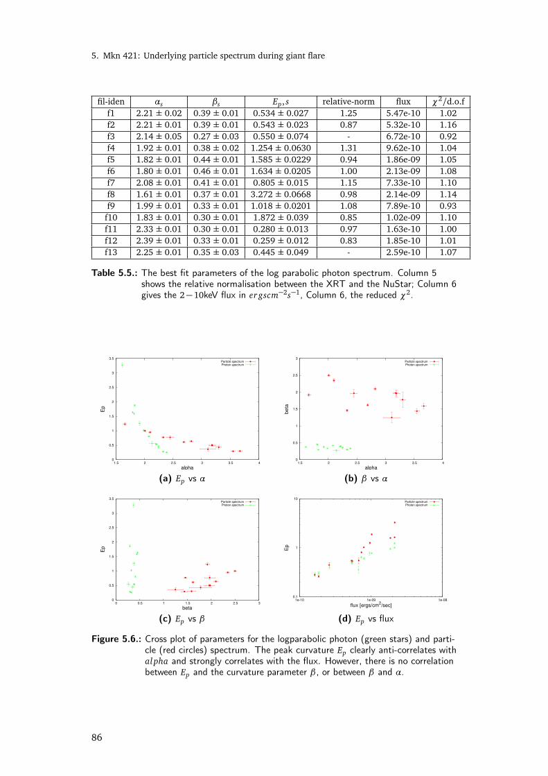
5. Mkn 421: Underlying particle spectrum during giant flare
fil-iden αs βs Ep, s relative-norm flux χ2/d.o.ff1 2.21 ± 0.02 0.39 ± 0.01 0.534 ± 0.027 1.25 5.47e-10 1.02f2 2.21 ± 0.01 0.39 ± 0.01 0.543 ± 0.023 0.87 5.32e-10 1.16f3 2.14 ± 0.05 0.27 ± 0.03 0.550 ± 0.074 - 6.72e-10 0.92f4 1.92 ± 0.01 0.38 ± 0.02 1.254 ± 0.0630 1.31 9.62e-10 1.04f5 1.82 ± 0.01 0.44 ± 0.01 1.585 ± 0.0229 0.94 1.86e-09 1.05f6 1.80 ± 0.01 0.46 ± 0.01 1.634 ± 0.0205 1.00 2.13e-09 1.08f7 2.08 ± 0.01 0.41 ± 0.01 0.805 ± 0.015 1.15 7.33e-10 1.10f8 1.61 ± 0.01 0.37 ± 0.01 3.272 ± 0.0668 0.98 2.14e-09 1.14f9 1.99 ± 0.01 0.33 ± 0.01 1.018 ± 0.0201 1.08 7.89e-10 0.93
f10 1.83 ± 0.01 0.30 ± 0.01 1.872 ± 0.039 0.85 1.02e-09 1.10f11 2.33 ± 0.01 0.30 ± 0.01 0.280 ± 0.013 0.97 1.63e-10 1.00f12 2.39 ± 0.01 0.33 ± 0.01 0.259 ± 0.012 0.83 1.85e-10 1.01f13 2.25 ± 0.01 0.35 ± 0.03 0.445 ± 0.049 - 2.59e-10 1.07
Table 5.5.: The best fit parameters of the log parabolic photon spectrum. Column 5shows the relative normalisation between the XRT and the NuStar; Column 6gives the 2−10keV flux in er gscm−2s−1, Column 6, the reduced χ2.
0
0.5
1
1.5
2
2.5
3
3.5
1.5 2 2.5 3 3.5 4
Ep
alpha
Particle spectrumPhoton spectrum
(a) Ep vs α
0
0.5
1
1.5
2
2.5
3
1.5 2 2.5 3 3.5 4
beta
alpha
Particle spectrumPhoton spectrum
(b) β vs α
0
0.5
1
1.5
2
2.5
3
3.5
0 0.5 1 1.5 2 2.5 3
Ep
beta
Particle spectrumPhoton spectrum
(c) Ep vs β
0.1
1
10
1e-10 1e-09 1e-08
Ep
flux [ergs/cm2/sec]
Particle spectrumPhoton spectrum
(d) Ep vs flux
Figure 5.6.: Cross plot of parameters for the logparabolic photon (green stars) and parti-cle (red circles) spectrum. The peak curvature Ep clearly anti-correlates withalpha and strongly correlates with the flux. However, there is no correlationbetween Ep and the curvature parameter β , or between β and α.
86

5.4. X-ray spectral analysis
δ. A good sampling of the entire SED from radio to γ-rays allows one to perform
a reasonable estimation of these physical parameters (Tavecchio et al., 1998). For
synchrotron emission alone, R, B, and δ will only decide the spectral normalization. On
the other hand, the shape of the observed spectrum is determined by the corresponding
form of the underlying particle spectrum. To obtain further insight into the emitting
particle distribution, we developed synchrotron emission models with different particle
distributions and incorporated them into XSPEC spectral fitting software. In particular,
we here consider the following particle distributions:
(i) Simple power law (SPL): In this case, we assume the electron distribution to be a
simple power law with a sharp high-energy cutoff, given by
N(γ)dγ= Kγ−pdγ, γ < γmax . (49)
Here γmc2 is the energy of the emitting electron, p is the particle spectral index,
K is the normalization, and γmax mc2 is the cut-off energy. Of these parameters, p
and γmax are chosen as the free parameters.
(ii) Cutoff power law (CPL) : Here the underlying particle distribution is assumed to be
a power law with index p and an exponential cutoff above energy γmmc2 given by
N(γ)dγ= Kγ−pex p(γ
γm)dγ. (50)
For this distribution, p and γm are chosen as the free parameters.
(iii) Broken power-law (BPL): The particle distribution in this case is described by a
broken power-law with indices p1 and p2 with a break at energy γb given by
N(γ)dγ=
¨
Kγ−p1 dγ, γmin < γ < γb
Kγ(p2−p1)b γ−p2 dγ, γb < γ < γmax
. (51)
Here, p1, p2 and γb are chosen as the free parameters.
(iv) Log parabola (LP): For this case, the particle distribution is chosen to be a log
parabola, given by
N(γ)dγ= K(γ/γb)−αp−βp log(γ/γb)dγ, (52)
with αp and βp chosen as the free parameters.
We fit the observed combined X-ray spectrum from Swift-XRT and NuSTAR with the
synchrotron emission due to these different particle distributions as given above, the
reduced χ2 of which are given in Table 5.6. As an example, we show the best fit
parameters corresponding to the state f5 in Table 5.7. A poor fit statistics with large
87

5. Mkn 421: Underlying particle spectrum during giant flare
4
4.2
4.4
4.6
4.8
5
5.2
5.4
1.6 1.8 2 2.2 2.4 2.6 2.8 3 3.2 3.4 3.6
p2
p1
Figure 5.7.: Cross plot of the two indices of the broken power-law particle spectrum. Thegreen points are not from combined spectrum, but are NuSTAR only andSwift-XRT only (see text).
reduced χ2 is encountered for the case of SPL since it fails to reproduce the smooth
curvature seen in almost all spectral states ( f 1− f 13). For CPL, the statistics improved
for many states with lowest reduced χ2 of 1.01 during state f3; whereas the largest
reduced χ2 is 1.41 for the state f6. The fit statistics improved considerably for many
states for the case of BPL except for f6 and f8, correspond to the peak of the X-ray flare.
In Figure 5.7 we show the cross-plot distribution of the power-law indices, p1 and p2, of
BPL model during different spectral states. The index p1 is poorly constrained for the
state f3 because we have no Swift-XRT observation during this period; whereas for state
f11 neither p1 nor p2 are well constrained because there are no NuSTAR observation.
However, for most of the states, a strong correlation between p1 and p2 is observed
(rs = 0.79 and p = 0.0018). Of all these particle distributions, the best statistics is
obtained for the LP model with the reduced χ2 decreased considerably during the flaring
states, f5, f6, and f8 (Table 5.6). Furthermore, the reduction of one free parameter in LP
with respect to BPL enforces the latter to be the most preferred particle distribution. In
Table 5.8 we list the best-fit parameters for the LP particle distribution.
We see similar correlations as discussed in Sect. 5.4.1. In fact, there is a linear
relationship between the parameters of the photon spectrum and the particle spectrum,
αp = 2.66αs + 2.66 (53)
βp = 6.49βs −0.51 (54)
88
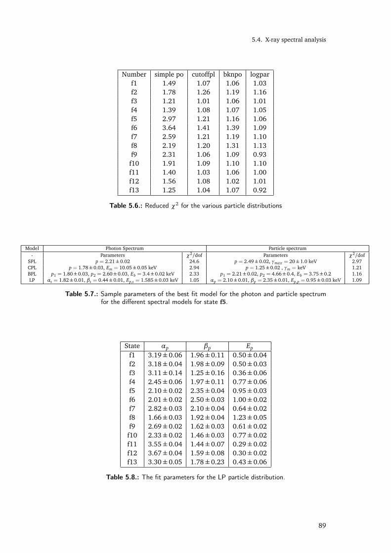
5.4. X-ray spectral analysis
Number simple po cutoffpl bknpo logparf1 1.49 1.07 1.06 1.03f2 1.78 1.26 1.19 1.16f3 1.21 1.01 1.06 1.01f4 1.39 1.08 1.07 1.05f5 2.97 1.21 1.16 1.06f6 3.64 1.41 1.39 1.09f7 2.59 1.21 1.19 1.10f8 2.19 1.20 1.31 1.13f9 2.31 1.06 1.09 0.93
f10 1.91 1.09 1.10 1.10f11 1.40 1.03 1.06 1.00f12 1.56 1.08 1.02 1.01f13 1.25 1.04 1.07 0.92
Table 5.6.: Reduced χ2 for the various particle distributions
Model Photon Spectrum Particle spectrum- Parameters χ2/dof Parameters χ2/dof
SPL p = 2.21±0.02 24.6 p = 2.49±0.02, γmax = 20±1.0 keV 2.97CPL p = 1.78±0.03, Em = 10.05±0.05 keV 2.94 p = 1.25±0.02 , γm = keV 1.21BPL p1 = 1.80±0.03, p2 = 2.60±0.03, Eb = 3.4±0.02 keV 2.33 p1 = 2.21±0.02, p2 = 4.66±0.4, Eb = 3.75±0.2 1.16LP αs = 1.82±0.01, βs = 0.44±0.01, Ep,s = 1.585±0.03 keV 1.05 αp = 2.10±0.01, βp = 2.35±0.01, Ep,p = 0.95±0.03 keV 1.09
Table 5.7.: Sample parameters of the best fit model for the photon and particle spectrumfor the different spectral models for state f5.
State αp βp Ep
f1 3.19±0.06 1.96±0.11 0.50±0.04f2 3.18±0.04 1.98±0.09 0.50±0.03f3 3.11±0.14 1.25±0.16 0.36±0.06f4 2.45±0.06 1.97±0.11 0.77±0.06f5 2.10±0.02 2.35±0.04 0.95±0.03f6 2.01±0.02 2.50±0.03 1.00±0.02f7 2.82±0.03 2.10±0.04 0.64±0.02f8 1.66±0.03 1.92±0.04 1.23±0.05f9 2.69±0.02 1.62±0.03 0.61±0.02f10 2.33±0.02 1.46±0.03 0.77±0.02f11 3.55±0.04 1.44±0.07 0.29±0.02f12 3.67±0.04 1.59±0.08 0.30±0.02f13 3.30±0.05 1.78±0.23 0.43±0.06
Table 5.8.: The fit parameters for the LP particle distribution.
89
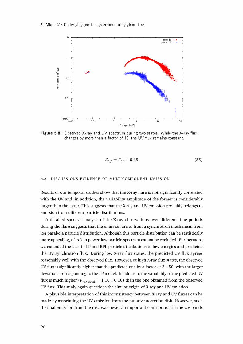
5. Mkn 421: Underlying particle spectrum during giant flare
0.001
0.01
0.1
1
10
0.001 0.01 0.1 1 10 100
νF
(ν)
[keV
/cm
2/s
ec]
Energy [keV]
state f6state f12
Figure 5.8.: Observed X-ray and UV spectrum during two states. While the X-ray fluxchanges by more than a factor of 10, the UV flux remains constant.
Ep,p = Ep,s + 0.35 (55)
5.5 D I S C U S S I O N S :E V I D E N C E O F M U LT I C O M P O N E N T E M I S S I O N
Results of our temporal studies show that the X-ray flare is not significantly correlated
with the UV and, in addition, the variability amplitude of the former is considerably
larger than the latter. This suggests that the X-ray and UV emission probably belongs to
emission from different particle distributions.
A detailed spectral analysis of the X-ray observations over different time periods
during the flare suggests that the emission arises from a synchrotron mechanism from
log parabola particle distribution. Although this particle distribution can be statistically
more appealing, a broken power-law particle spectrum cannot be excluded. Furthermore,
we extended the best-fit LP and BPL particle distributions to low energies and predicted
the UV synchrotron flux. During low X-ray flux states, the predicted UV flux agrees
reasonably well with the observed flux. However, at high X-ray flux states, the observed
UV flux is significantly higher that the predicted one by a factor of 2−50, with the larger
deviations corresponding to the LP model. In addition, the variability of the predicted UV
flux is much higher (Fvar,pred = 1.10±0.10) than the one obtained from the observed
UV flux. This study again questions the similar origin of X-ray and UV emission.
A plausible interpretation of this inconsistency between X-ray and UV fluxes can be
made by associating the UV emission from the putative accretion disk. However, such
thermal emission from the disc was never an important contribution in the UV bands
90
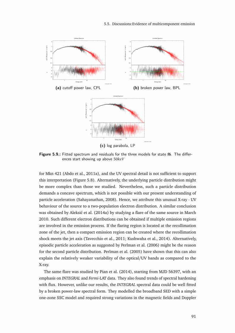
5.5. Discussions:Evidence of multicomponent emission
0.1
1
0.2
0.5
2
ke
V2 (
Ph
oto
ns c
m−
2 s
−1 k
eV
−1)
Unfolded Spectrum
1 10
−4
−2
0
2
χ
Energy (keV)
9−Oct−2014 15:01
(a) cutoff power law, CPL
0.1
1
0.2
0.5
2
ke
V2 (
Ph
oto
ns c
m−
2 s
−1 k
eV
−1)
Unfolded Spectrum
1 10
−4
−2
0
2
χ
Energy (keV)
9−Oct−2014 15:00
(b) broken power law, BPL
0.1
1
0.2
0.5
2
ke
V2 (
Ph
oto
ns c
m−
2 s
−1 k
eV
−1)
Unfolded Spectrum
1 10
−2
0
2
χ
Energy (keV)
9−Oct−2014 15:00
(c) log parabola, LP
Figure 5.9.: Fitted spectrum and residuals for the three models for state f6. The differ-ences start showing up above 50keV
for Mkn 421 (Abdo et al., 2011a), and the UV spectral detail is not sufficient to support
this interpretation (Figure 5.8). Alternatively, the underlying particle distribution might
be more complex than those we studied. Nevertheless, such a particle distribution
demands a concave spectrum, which is not possible with our present understanding of
particle acceleration (Sahayanathan, 2008). Hence, we attribute this unusual X-ray - UV
behaviour of the source to a two-population electron distribution. A similar conclusion
was obtained by Aleksic et al. (2014a) by studying a flare of the same source in March
2010. Such different electron distributions can be obtained if multiple emission regions
are involved in the emission process. If the flaring region is located at the recollimation
zone of the jet, then a compact emission region can be created where the recollimation
shock meets the jet axis (Tavecchio et al., 2011; Kushwaha et al., 2014). Alternatively,
episodic particle acceleration as suggested by Perlman et al. (2006) might be the reason
for the second particle distribution. Perlman et al. (2005) have shown that this can also
explain the relatively weaker variability of the optical/UV bands as compared to the
X-ray.
The same flare was studied by Pian et al. (2014), starting from MJD 56397, with an
emphasis on INTEGRAL and Fermi-LAT data. They also found trends of spectral hardening
with flux. However, unlike our results, the INTEGRAL spectral data could be well fitted
by a broken power-law spectral form. They modelled the broadband SED with a simple
one-zone SSC model and required strong variations in the magnetic fields and Doppler
91
5. Mkn 421: Underlying particle spectrum during giant flare
factors to sucessfully fit the SED of different states. In addition, our results do not match
those of Massaro et al. (2004) because we found no correlation between αs and βs. Thus,
our results are inconsistent with statistical particle acceleration.
Our results indicate the potential of using broadband X-ray data to constrain the
underlying particle spectrum and distinguish separate variable spectral components,
especially if there are simultaneous data in other wavebands. Figure 5.9 shows the
energy spectrum (in νFν) and the residuals for the BPL, the CPL and the LP for the state
f6. While the residuals show structure as a function of energy for energies < 0.7keV,
especially for the CPL and the BPL, the data and model agree within 10% at these energies.
Moreover, we also implemented a fit at energies < 0.7keV and verified that our results
do not change significantly. Thus, this effect is unlikely to be a serious source of error in
this work. More importantly, there is a clear systematic deviation from the data for the
BPL and the CPL at the higher energies, beyond 50keV .
5.6 C O N C LU S I O N S
We performed a detailed study of the bright X-ray flare of Mkn 421 observed in April
2013 along with information available at other wavebands, which showed that the X-ray
flares were probably caused by a separate population that did not contribute significantly
to the radiation at lower energies. The major focus of the work has been to demonstrate
that, with broadband X-ray spectral coverage, it is directly possible to distinguish between
models of the emitting particle spectra. Now that ASTROSAT has started observations,
we can have excellent simultaneous X-ray spectra from 0.3 to around 80 keV for a handful
of blazars. Application of this technique to the same can throw new light on the emission
mechanisms in these large scale jets.
92

“Imagination will often carry us to worlds that never were.
But without it we go nowhere."
Carl Sagan
61ES 1011+496: Effect of spatial
particle diffusion on spectralcurvature
1ES 1011+496 (RA: 10 15’ 04.1"; Dec:49 26’ 01"; J2000) is a HBL located at a redshift
of z = 0.212. It was discovered as a VHE emitter by the MAGIC collaboration in 2007,
following an optical outburst in March 2007 (Albert et al., 2007b). At its epoch of
discovery, it was the furthest known TeV source, and is often used to constrain the EBL
density (Ahnen et al., 2016b). In this chapter, we perform a detailed multi-epoch study
of the broadband spectral behaviour of this source, which provides us with valuable
information regarding the underlying particle distribution (Sinha et al., 2016a).
6.1 I N T R O D U C T I O N
1ES 1011+496 was discovered as a VHE emitter by the MAGIC collaboration in 2007,
following an optical outburst in March 2007 (Albert et al., 2007b). Using the Blue
Channel Spectrograph at the Multi Mirror Telescope Brusa et al. (2003), the redshift of
the source was determined to be z = 0.212±0.002 (Figure 6.1). The flux above 200
GeV was roughly 7% of the Crab Nebula, and the observed spectrum was reported to
be a power law with a very steep index of 4.0± 0.5. After correction for attenuation
of VHE photons by photons of the EBL (Kneiske & Dole, 2010), the intrinsic spectral
index was computed to be 3.3±0.7 (Figure 6.2a).Albert et al. (2007b) constructed the
SED (Figure 6.2b) with simultaneous optical R-band data, and other historical data from
Costamante & Ghisellini (2002) and modelled it with a single zone radiating via SSC
processes. However, the model parameters could not be constrained due to the sparse
sampling and the non-simultaneity of the data. Hartman et al. (1999) had suggested the
93
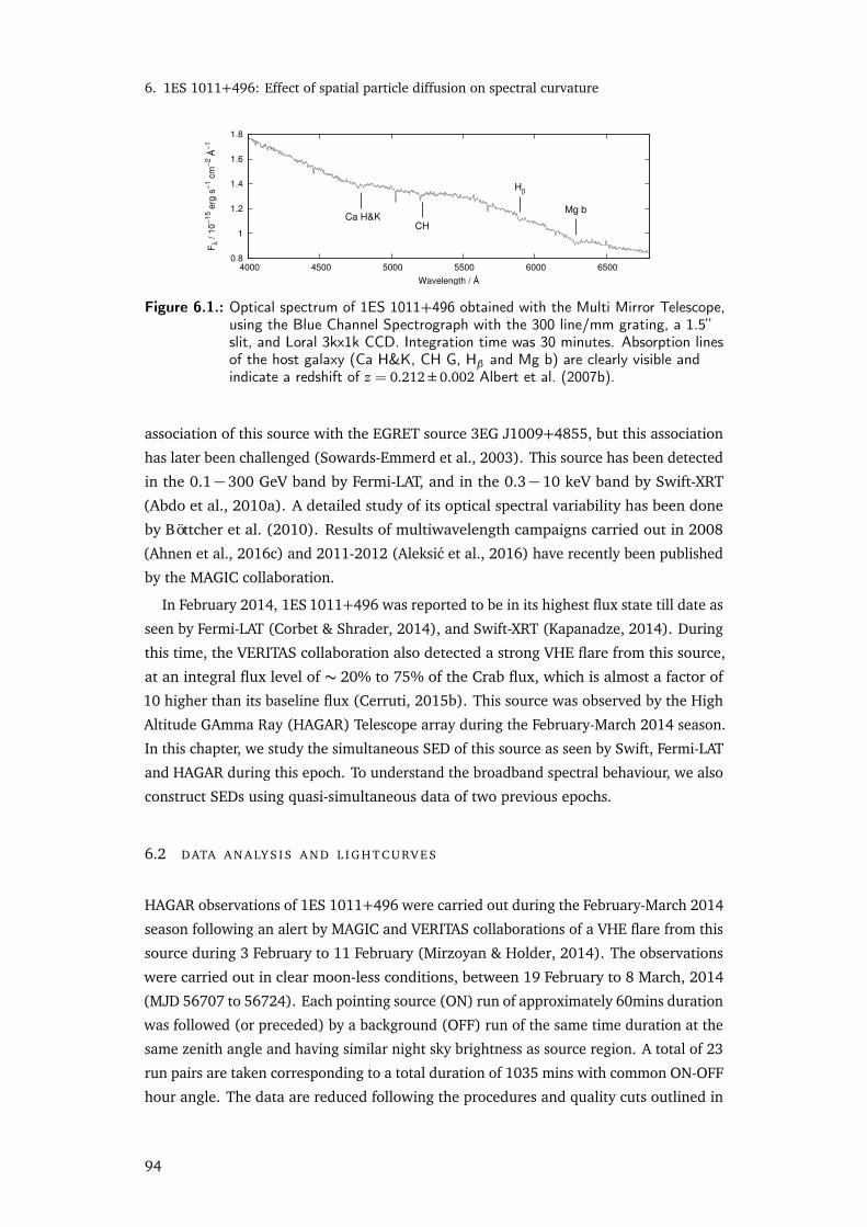
6. 1ES 1011+496: Effect of spatial particle diffusion on spectral curvature
0.8
1
1.2
1.4
1.6
1.8
4000 4500 5000 5500 6000 6500
Fλ /
10−1
5 erg
s−1
cm
−2 Å
−1
Wavelength / Å
Hβ
Ca H&KCH
Mg b
Figure 6.1.: Optical spectrum of 1ES 1011+496 obtained with the Multi Mirror Telescope,using the Blue Channel Spectrograph with the 300 line/mm grating, a 1.5”slit, and Loral 3kx1k CCD. Integration time was 30 minutes. Absorption linesof the host galaxy (Ca H&K, CH G, Hβ and Mg b) are clearly visible andindicate a redshift of z = 0.212±0.002 Albert et al. (2007b).
association of this source with the EGRET source 3EG J1009+4855, but this association
has later been challenged (Sowards-Emmerd et al., 2003). This source has been detected
in the 0.1− 300 GeV band by Fermi-LAT, and in the 0.3− 10 keV band by Swift-XRT
(Abdo et al., 2010a). A detailed study of its optical spectral variability has been done
by Böttcher et al. (2010). Results of multiwavelength campaigns carried out in 2008
(Ahnen et al., 2016c) and 2011-2012 (Aleksic et al., 2016) have recently been published
by the MAGIC collaboration.
In February 2014, 1ES 1011+496 was reported to be in its highest flux state till date as
seen by Fermi-LAT (Corbet & Shrader, 2014), and Swift-XRT (Kapanadze, 2014). During
this time, the VERITAS collaboration also detected a strong VHE flare from this source,
at an integral flux level of ∼ 20% to 75% of the Crab flux, which is almost a factor of
10 higher than its baseline flux (Cerruti, 2015b). This source was observed by the High
Altitude GAmma Ray (HAGAR) Telescope array during the February-March 2014 season.
In this chapter, we study the simultaneous SED of this source as seen by Swift, Fermi-LAT
and HAGAR during this epoch. To understand the broadband spectral behaviour, we also
construct SEDs using quasi-simultaneous data of two previous epochs.
6.2 DATA A N A LY S I S A N D L I G H T C U RV E S
HAGAR observations of 1ES 1011+496 were carried out during the February-March 2014
season following an alert by MAGIC and VERITAS collaborations of a VHE flare from this
source during 3 February to 11 February (Mirzoyan & Holder, 2014). The observations
were carried out in clear moon-less conditions, between 19 February to 8 March, 2014
(MJD 56707 to 56724). Each pointing source (ON) run of approximately 60mins duration
was followed (or preceded) by a background (OFF) run of the same time duration at the
same zenith angle and having similar night sky brightness as source region. A total of 23
run pairs are taken corresponding to a total duration of 1035 mins with common ON-OFF
hour angle. The data are reduced following the procedures and quality cuts outlined in
94

6.2. Data analysis and lightcurves
Energy, E [GeV]100 200 300 400 500 1000
]-1
s-2
cm
-1d
iffe
ren
tial fl
ux, d
N/d
E [
TeV
-1310
-1210
-1110
-1010
-910
-810
MAGIC, 1ES1011+496
power law fit:Γ-
200GeVE
0dN/dE = N
]-1 s-2 cm-1 [TeV-10
10× 0.1)± = (2.0 0N
0.5± = 4.0 Γ
1ES1011+496, measured
Power law fit to data
1ES1011+496, deabsorbed
Crab Nebula spectrum
(a) TeV spectrum (b) Broadband SED
Figure 6.2.: Detected TeV spectrum and the constructed SED by Albert et al. (2007b).(a) The measured spectrum (black filled circles), the power-law fit to thedata (solid line), the deabsorbed spectrum (brown open circles), and the fitto the deabsorbed spectrum (dashed brown line). The last measured pointis a 95% upper limit. In the deabsorbed spectrum, the last spectral point at≈600GeV is 1.6σ above the fit and thus not significant. The Crab Nebulaspectrum (green dashed line, Aharonian et al. (2000)) is shown for compari-son.(b) Spectral energy distribution of 1ES 1011+496. The two different fits aredone by varying the minimum electron energy γmin (see text). The otherfit parameters are: R(radius of sphere)=1016 cm, δ(Doppler factor)=20,B(magnetic field) = 0.15G, γmax(maximum electron Lorentz factor)= 2 ·107
γb(break electron Lorenz factor)= 5 · 104 the slopes of the electron distribu-tion n1 = 2 and n2 = 5 before and after the break energy, respectively, aswell as ne(normalization of the electron energy distribution) = 2 · 104 cm−3.The model is not intended for describing the radio data, which is assumed tooriginate from a larger emitting volume to avoid an intrinsic absorption.
state Start date End date XRT obs id XRT exp XRT spectral parameters LAT spectral parametersISO ISO time (ks) α β F2−10 keV Index F0.2−300 GeV
s1 2012-03-19 2012-04-03
00035012020
6.3 2.27±0.19 0.17±0.10 1.6±0.3 1.81±0.16 4.3±0.9000350120210003501202200035012023
s2 2012-12-19 2013-01-18
00035012024
5.1 2.37±0.11 0.61±0.22 0.82±0.07 1.74±0.13 2.8±0.60003501202500035012026000350120270003501202800035012029
s3 2014-02-04 2014-03-04
00035012030
7.3 1.94±0.04 0.16±0.0.03 4.11±0.12 1.77±0.22 9.8±0.30003501203100035012032000350120330003501203500035012036
Table 6.1.: Observation details (XRT observation ids and the total exposure time) andspectral parameters in the X-ray and GeV bands for the different states forwhich the SED has been extracted. The X-ray 2− 10 keV flux is quoted in10−11 ergs/cm2/s, and the Fermi-LAT 0.2−300 GeV flux in 10−8 ph/cm2/s.
95
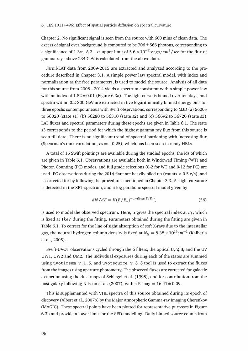
6. 1ES 1011+496: Effect of spatial particle diffusion on spectral curvature
Chapter 2. No significant signal is seen from the source with 600 mins of clean data. The
excess of signal over background is computed to be 706±566 photons, corresponding to
a significance of 1.3σ. A 3−σ upper limit of 5.6×10⁻¹¹er gs/cm2/sec for the flux of
gamma rays above 234 GeV is calculated from the above data.
Fermi-LAT data from 2009-2015 are extracted and analyzed according to the pro-
cedure described in Chapter 3.1. A simple power law spectral model, with index and
normalization as the free parameters, is used to model the source. Analysis of all data
for this source from 2008 - 2014 yields a spectrum consistent with a simple power law
with an index of 1.82±0.01 (Figure 6.3a). The light curve is binned over ten days, and
spectra within 0.2-300 GeV are extracted in five logarithmically binned energy bins for
three epochs contemporaneous with Swift observations, corresponding to MJD (a) 56005
to 56020 (state s1) (b) 56280 to 56310 (state s2) and (c) 56692 to 56720 (state s3).
LAT fluxes and spectral parameters during these epochs are given in Table 6.1. The state
s3 corresponds to the period for which the highest gamma ray flux from this source is
seen till date. There is no significant trend of spectral hardening with increasing flux
(Spearman’s rank correlation, rs = −0.25), which has been seen in many HBLs.
A total of 16 Swift pointings are available during the studied epochs, the ids of which
are given in Table 6.1. Observations are available both in Windowed Timing (WT) and
Photon Counting (PC) modes, and full grade selections (0-2 for WT and 0-12 for PC) are
used. PC observations during the 2014 flare are heavily piled up (counts > 0.5 c/s), and
is corrected for by following the procedures mentioned in Chapter 3.3. A slight curvature
is detected in the XRT spectrum, and a log parabolic spectral model given by
dN/dE = K(E/Eb)−α−β log(E/Eb), (56)
is used to model the observed spectrum. Here, α gives the spectral index at Eb, which
is fixed at 1keV during the fitting. Parameters obtained during the fitting are given in
Table 6.1. To correct for the line of sight absorption of soft X-rays due to the interstellar
gas, the neutral hydrogen column density is fixed at NH = 8.38×1019cm−2 (Kalberla
et al., 2005).
Swift-UVOT observations cycled through the 6 filters, the optical U, V, B, and the UV
UW1, UW2 and UM2. The individual exposures during each of the states are summed
using uvotimsum v.1.6, and uvotsource v.3.3 tool is used to extract the fluxes
from the images using aperture photometry. The observed fluxes are corrected for galactic
extinction using the dust maps of Schlegel et al. (1998), and for contribution from the
host galaxy following Nilsson et al. (2007), with a R-mag = 16.41±0.09.
This is supplemented with VHE spectra of this source obtained during its epoch of
discovery (Albert et al., 2007b) by the Major Atmospheric Gamma-ray Imaging Cherenkov
(MAGIC). These spectral points have been plotted for representative purposes in Figure
6.3b and provide a lower limit for the SED modelling. Daily binned source counts from
96
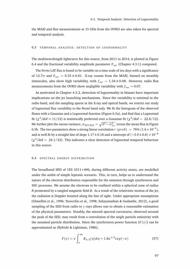
6.3. Temporal Analysis: Detection of Lognormality
the MAXI and flux measurements at 15 GHz from the OVRO are also taken for spectral
and temporal analysis.
6.3 T E M P O R A L A N A LY S I S : D E T E C T I O N O F L O G N O R M A L I T Y
The multiwavelength lightcurve for this source, from 2011 to 2014, is plotted in Figure
6.4 and the fractional variability amplitude parameter Fvar (Chapter 4.3.1) computed.
The Fermi-LAT flux is found to be variable on a time scale of ten days with a significance
of 12.7σ and Fvar = 0.35± 0.01. X-ray counts from the MAXI, binned on monthly
timescales, also show high variability, with fvar = 1.34± 0.08. However, radio flux
measurements from the OVRO show negligible variability with fvar ∼ 0.07.
As motivated in Chapter 4.3.2, detection of lognormality in blazars have important
implications on the jet launching mechanisms. Since the variability is minimal in the
radio band, and the sampling sparse in the X-ray and optical bands, we restrict our study
of lognormal flux variability to the Fermi band only. We fit the histogram of the observed
fluxes with a Gaussian and a Lognormal function (Figure 6.5a), and find that a Lognormal
fit (χ2/dof = 11/12) is statistically preferred over a Gaussian fit (χ2/dof = 22.8/12).
We further plot the excess variance,σEX C ESS =Æ
S2−σ2er r versus the mean flux in Figure
6.5b. The two parameters show a strong linear correlation r (prob) = 76% (1.6×10⁻⁵),
and is well fit by a straight line of slope 1.17±0.18 and a intercept of (−3.9±0.8)×10−8
(χ2/dof = 24.1/22). This indicates a clear detection of lognormal temporal behaviour
in this source.
6.4 S P E C T R A L E N E R GY D I S T R I B U T I O N
The broadband SED of 1ES 1011+496, during different activity states, are modelled
under the ambit of simple leptonic scenario. This, in turn, helps us to understand the
nature of the electron distribution responsible for the emission through synchrotron and
SSC processes. We assume the electrons to be confined within a spherical zone of radius
R permeated by a tangled magnetic field B. As a result of the relativistic motion of the jet,
the radiation is Doppler boosted along the line of sight. Under appropriate assumptions
(Ghisellini et al., 1996; Tavecchio et al., 1998; Sahayanathan & Godambe, 2012), a good
sampling of the SED from radio to γ-rays allows one to obtain a reasonable estimation
of the physical parameters. Notably, the smooth spectral curvatures, observed around
the peak of the SED, may result from a convolution of the single particle emissivity with
the assumed particle distribution. Since the synchrotron power function (F(x)) can be
approximated as (Rybicki & Lightman, 1986),
F(x) = x
∫ ∞
xK5/3(η)dη∼ 1.8x1/3ex p(−x) (57)
97
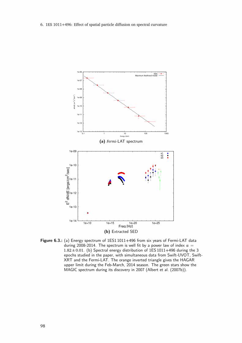
6. 1ES 1011+496: Effect of spatial particle diffusion on spectral curvature
1e-13
1e-12
1e-11
1e-10
1e-09
1e-08
1e-07
1e-06
0.1 1 10 100 1000
dN
/dE
(cm
-2s
-1G
eV
-1)
Energy (GeV)
dataMaximum likelihood model
(a) Fermi-LAT spectrum
1e-14
1e-13
1e-12
1e-11
1e-10
1e-09
1e+10 1e+15 1e+20 1e+25
E2 d
N/d
E [
erg
s/c
m2/s
ec]
Freq [Hz]
s1s2s3
(b) Extracted SED
Figure 6.3.: (a) Energy spectrum of 1ES1 1011+496 from six years of Fermi-LAT dataduring 2008-2014. The spectrum is well fit by a power law of index α =1.82± 0.01. (b) Spectral energy distribution of 1ES 1011+496 during the 3epochs studied in the paper, with simultaneous data from Swift-UVOT, Swift-XRT and the Fermi-LAT. The orange inverted triangle gives the HAGARupper limit during the Feb-March, 2014 season. The green stars show theMAGIC spectrum during its discovery in 2007 (Albert et al. (2007b)).
98
6.4. Spectral Energy Distribution
0.2
0.3
0.4
[Jy]
s1
s2
s3
s1 s2 s3s1
s2
s3
s1 s2 s3
OVRO
1.2
1.6
[mJy]
Optical U
0.6
0.9
[mJy]
UV UW2
-0.04
0
0.04
cts
/s
MAXI
2
4
6
cts
/s
Swift-XRT
0
1
55600 55800 56000 56200 56400 56600 56800
10
7 p
h/s
MJD
Fermi-LAT
Figure 6.4.: Multiwavelength lightcurve during MJD 55600 to 56800 (calendar days 2011-2014) showing from top: Panel 1: OVRO flux in Jy; Panel 2: Optical U bandflux in mJy; Panel 3: UV flux in UW2 band in mJy; Panel 4: MAXI flux (withmonthly binning) in counts/sec; Panel 5: Swift-XRT flux in counts/sec; Panel6: Fermi-LAT flux (with 10 days binning) in ph/cm2/sec. The three statesfor which SED has been studied are marked and labelled as s1, s2 and s3respectively.
99

6. 1ES 1011+496: Effect of spatial particle diffusion on spectral curvature
Flux [ph/cm^2/sec]
0 0.05 0.1 0.15 0.2
610×
Fre
quency
0
10
20
30
40
50 FermiLAT
(a) Flux distribution
0
2e-08
4e-08
6e-08
4e-08 6e-08 8e-08
σ [
ph/c
m2/s
ec]
Flux [ph/cm2/sec]
(b) Flux-rms relation
Figure 6.5.: Detection of lognormality in 1ES 1011+496 in the Fermi energy band. Thefirst panel shows the histogram of the observed fluxes (black points) fittedwith a Gaussian (dotted blue line) and Lognormal (solid red line) function.A Lognormal fit is clearly preferred. The second panel shows the strong lin-ear relationship seen between the flux and the excess rms. The black pointsdenote data points averaged over 100days, and the solid gray line the linearfit.
100
6.4. Spectral Energy Distribution
a sharp break in the particle spectrum will give rise to a smooth curvature in the
photon spectrum. On the other hand, the underlying particle distribution itself can show
a gradual transition causing the observed curvatures. To investigate this, we model the
observed SED with the following choices of particle distributions:
(i) Broken Power Law (BPL): In this case, we assume the electron spectrum to be a
sharp broken power law with indices p and q, given by
N(γ)dγ=
¨
N0γ−pdγ, γmin < γ < γb
N0γ(q−p)b γ−qdγ, γb < γ < γmax
(58)
(ii) Smooth Broken Power law (SBPL): Here, the electron distribution is a smooth broken
power law with low energy index p and the high energy index q.
N(γ)dγ= N0(γb)
−p
(γ/γb)p +(γ/γb)qdγ, γmin < γ < γmax (59)
(iii) Power law with an exponential cutoff (CPL): The particle distribution in this case is
chosen to be a power law with index p and an exponentially decreasing tail, given
by
N(γ)dγ= N0γ−pex p
−γ
γb
dγ, γmin < γ < γmax (60)
Here, γmin and γmax are the minimum and maximum dimensionless energy (E = γmc2)
of the non-thermal electron distribution, γb the electron energy associated with the
peak of the SED and N0 the normalization. To reduce the number of unknowns, the
radius R is fixed at 1.3× 1016cm, corresponding to a variability time scale of tvar ≈ 1
day (for the Doppler factor δ ≈ 10). In addition, the magnetic field energy density,
UB
= B2
8π
, is considered to be in equipartition with the particle energy density (Ue).
The resultant model spectra, corresponding to epoch s3, for the above three choices
of particle distribution are shown in Figure 6.7, along with the observed fluxes. The
governing physical parameters are given in Table 6.2.
Our study shows that the commonly used electron spectrum, the BPL [e.g. Ghisellini
et al. (1996); Krawczynski et al. (2004)], cannot explain the smooth curvature observed
at the X-ray energies for this source implying that the synchrotron emissivity function
alone is not sufficient to give rise to the observed curvature, and that the underlying
particle spectrum itself must have a gradual transition as opposed to a sharp break. This
suggests that the SBPL and CPL are the better choices to represent the observed SED and
in Figure 6.6 we show the model spectra corresponding to these particle distributions
for all the three epochs considered in this study. Both these models can well reproduce
the observed spectrum, during all three epochs, and the absence of simultaneous hard
X-ray and TeV measurements prevents us from distinguishing between the two models.
Particularly, with the current sampling, the index q and the γmax for the SBPL cannot
101
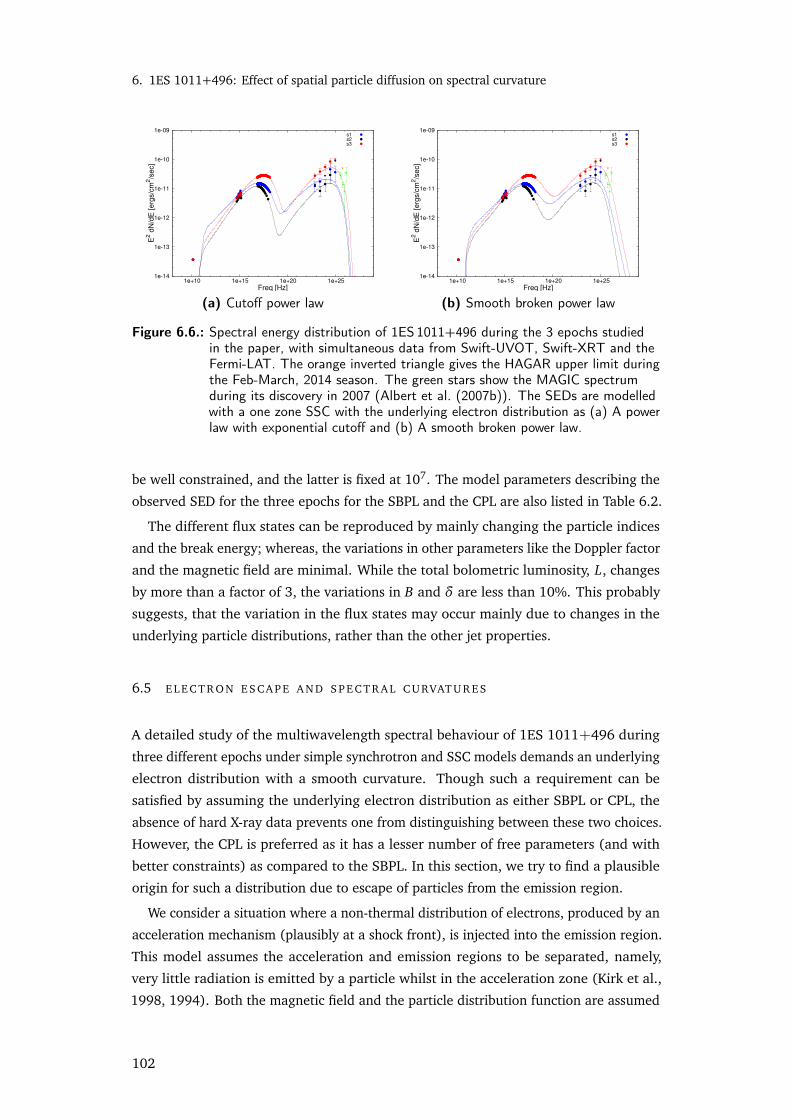
6. 1ES 1011+496: Effect of spatial particle diffusion on spectral curvature
1e-14
1e-13
1e-12
1e-11
1e-10
1e-09
1e+10 1e+15 1e+20 1e+25
E2 d
N/d
E [erg
s/c
m2/s
ec]
Freq [Hz]
s1s2s3
(a) Cutoff power law
1e-14
1e-13
1e-12
1e-11
1e-10
1e-09
1e+10 1e+15 1e+20 1e+25
E2 d
N/d
E [erg
s/c
m2/s
ec]
Freq [Hz]
s1s2s3
(b) Smooth broken power law
Figure 6.6.: Spectral energy distribution of 1ES 1011+496 during the 3 epochs studiedin the paper, with simultaneous data from Swift-UVOT, Swift-XRT and theFermi-LAT. The orange inverted triangle gives the HAGAR upper limit duringthe Feb-March, 2014 season. The green stars show the MAGIC spectrumduring its discovery in 2007 (Albert et al. (2007b)). The SEDs are modelledwith a one zone SSC with the underlying electron distribution as (a) A powerlaw with exponential cutoff and (b) A smooth broken power law.
be well constrained, and the latter is fixed at 107. The model parameters describing the
observed SED for the three epochs for the SBPL and the CPL are also listed in Table 6.2.
The different flux states can be reproduced by mainly changing the particle indices
and the break energy; whereas, the variations in other parameters like the Doppler factor
and the magnetic field are minimal. While the total bolometric luminosity, L, changes
by more than a factor of 3, the variations in B and δ are less than 10%. This probably
suggests, that the variation in the flux states may occur mainly due to changes in the
underlying particle distributions, rather than the other jet properties.
6.5 E L E C T R O N E S CA P E A N D S P E C T R A L C U RVAT U R E S
A detailed study of the multiwavelength spectral behaviour of 1ES 1011+496 during
three different epochs under simple synchrotron and SSC models demands an underlying
electron distribution with a smooth curvature. Though such a requirement can be
satisfied by assuming the underlying electron distribution as either SBPL or CPL, the
absence of hard X-ray data prevents one from distinguishing between these two choices.
However, the CPL is preferred as it has a lesser number of free parameters (and with
better constraints) as compared to the SBPL. In this section, we try to find a plausible
origin for such a distribution due to escape of particles from the emission region.
We consider a situation where a non-thermal distribution of electrons, produced by an
acceleration mechanism (plausibly at a shock front), is injected into the emission region.
This model assumes the acceleration and emission regions to be separated, namely,
very little radiation is emitted by a particle whilst in the acceleration zone (Kirk et al.,
1998, 1994). Both the magnetic field and the particle distribution function are assumed
102
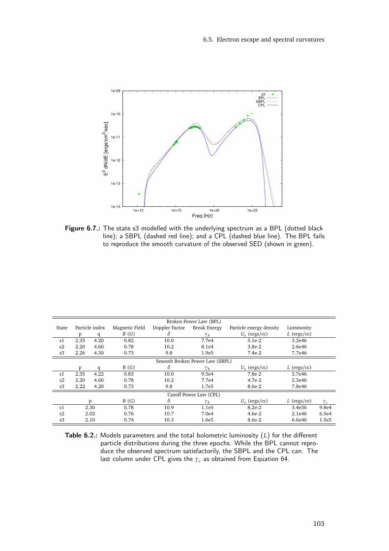
6.5. Electron escape and spectral curvatures
1e-14
1e-13
1e-12
1e-11
1e-10
1e-09
1e+10 1e+15 1e+20 1e+25
E2 d
N/d
E [erg
s/c
m2/s
ec]
Freq [Hz]
s3BPL
SBPLCPL
Figure 6.7.: The state s3 modelled with the underlying spectrum as a BPL (dotted blackline); a SBPL (dashed red line); and a CPL (dashed blue line). The BPL failsto reproduce the smooth curvature of the observed SED (shown in green).
Broken Power Law (BPL)State Particle index Magnetic Field Doppler Factor Break Energy Particle energy density Luminosity
p q B (G) δ γb Ue (ergs/cc) L (ergs/cc)s1 2.35 4.20 0.82 10.0 7.7e4 5.1e-2 3.2e46s2 2.20 4.60 0.78 10.2 8.1e4 3.8e-2 2.6e46s3 2.26 4.30 0.73 9.8 1.9e5 7.4e-2 7.7e46
Smooth Broken Power Law (SBPL)p q B (G) δ γb Ue (ergs/cc) L (ergs/cc)
s1 2.35 4.22 0.83 10.0 9.5e4 7.8e-2 3.7e46s2 2.20 4.60 0.78 10.2 7.7e4 4.7e-2 2.3e46s3 2.22 4.20 0.73 9.8 1.7e5 8.6e-2 7.8e46
Cutoff Power Law (CPL)p B (G) δ γb Ue (ergs/cc) L (ergs/cc) γc
s1 2.30 0.78 10.9 1.1e5 8.2e-2 3.4e36 9.8e4s2 2.02 0.76 10.7 7.0e4 4.6e-2 2.1e46 6.5e4s3 2.10 0.74 10.3 1.6e5 8.6e-2 6.6e46 1.5e5
Table 6.2.: Models parameters and the total bolometric luminosity (L) for the differentparticle distributions during the three epochs. While the BPL cannot repro-duce the observed spectrum satisfactorily, the SBPL and the CPL can. Thelast column under CPL gives the γc as obtained from Equation 64.
103

6. 1ES 1011+496: Effect of spatial particle diffusion on spectral curvature
homogeneous throughout the emission region. The electrons leave the emission region
at some characteristic time scale, tesc, and after escape, a particle no longer radiates.
The particle number density, N(γ, t), with Lorentz factors between γ and γ+ dγ in the
emission region can then be conveniently described by the kinetic equation (Kardashev,
1962)∂ N∂ t−∂
∂ γ(P(γ)N)+
Ntesc(γ)
= Q(γ)Θ(γ−γmax )δ(t − t0) (61)
where P(γ) is the energy loss rate due to synchrotron and SSC processes, and Q(γ) =
Q0γ−p is the power law distribution of electrons injected by the acceleration process at
time t0 with maximum injected electron energy being γmax .
6.5.1 Analytic solution: Thomson scattering
For a time independent energy loss rate P = P(γ), and an energy dependent escape
rate, tesc = (τγξ), Equation 61 can be analytically solved when the Inverse Compton
scattering is confined to the Thomson regime following the Green’s function method
outlined in Section 3.2 of Atoyan & Aharonian (1999),
N(γ, t) =KΓ 2−p
0
γ2exp
−∫ t
0
d xτ(Γx )
(62)
where
t − x =
∫ Γx (γ,t)
γ
dγP(γ)
(63)
is the trajectory of the particle in energy space.
The final solution is obtained as
N(γ, t) =
Q0Γ2−p0
γ2exp
−γmaxγ
ξc
(ξ+ 1)
1γ
ξ+1
−
1γ−
1γmax
ξ+1
; for ξ 6= −1
Q0Γ2−p0
γ2
1−γ
γmax
γbγc
; for ξ= −1
(64)
Here Γ0 = (1/γ−1/γmax )−1 is the energy of the electron at t0 evolving to γ at t, and
γc(t) = (t/τ)1/ξ is the characteristic energy below which particles have not diffused
out of the emission region.
6.5.2 Numerical solution: Klein-Nishina scattering
However, detection of the source at VHE energies suggests that the Thomson scattering ap-
proximation of SSC process may not be valid and one needs to incorporate Klein-Nishina
(KN) correction in the cross-section (Tavecchio et al., 1998). Hence, we numerically
104
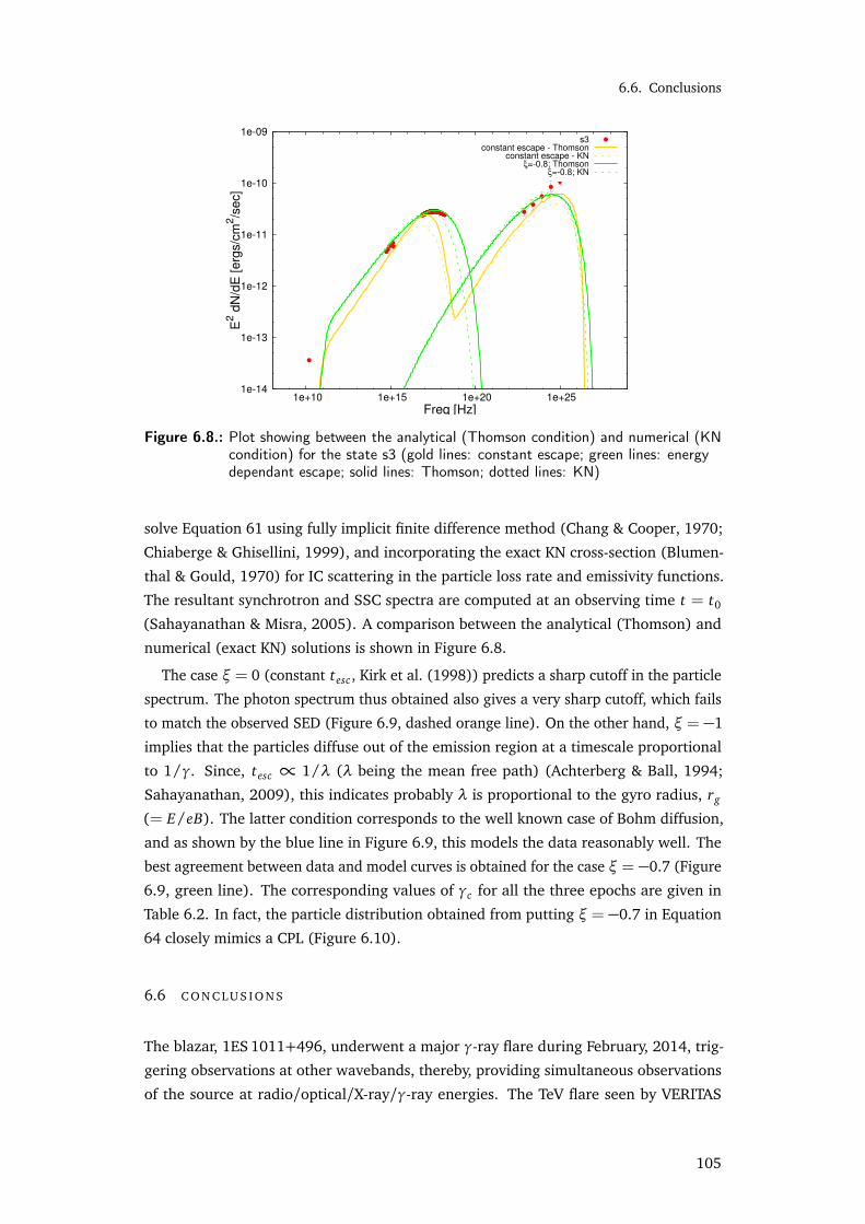
6.6. Conclusions
1e-14
1e-13
1e-12
1e-11
1e-10
1e-09
1e+10 1e+15 1e+20 1e+25
E2 d
N/d
E [erg
s/c
m2/s
ec]
Freq [Hz]
s3constant escape - Thomson
constant escape - KNξ=-0.8; Thomson
ξ=-0.8; KN
Figure 6.8.: Plot showing between the analytical (Thomson condition) and numerical (KNcondition) for the state s3 (gold lines: constant escape; green lines: energydependant escape; solid lines: Thomson; dotted lines: KN)
solve Equation 61 using fully implicit finite difference method (Chang & Cooper, 1970;
Chiaberge & Ghisellini, 1999), and incorporating the exact KN cross-section (Blumen-
thal & Gould, 1970) for IC scattering in the particle loss rate and emissivity functions.
The resultant synchrotron and SSC spectra are computed at an observing time t = t0
(Sahayanathan & Misra, 2005). A comparison between the analytical (Thomson) and
numerical (exact KN) solutions is shown in Figure 6.8.
The case ξ= 0 (constant tesc , Kirk et al. (1998)) predicts a sharp cutoff in the particle
spectrum. The photon spectrum thus obtained also gives a very sharp cutoff, which fails
to match the observed SED (Figure 6.9, dashed orange line). On the other hand, ξ= −1
implies that the particles diffuse out of the emission region at a timescale proportional
to 1/γ. Since, tesc ∝ 1/λ (λ being the mean free path) (Achterberg & Ball, 1994;
Sahayanathan, 2009), this indicates probably λ is proportional to the gyro radius, rg
(= E/eB). The latter condition corresponds to the well known case of Bohm diffusion,
and as shown by the blue line in Figure 6.9, this models the data reasonably well. The
best agreement between data and model curves is obtained for the case ξ= −0.7 (Figure
6.9, green line). The corresponding values of γc for all the three epochs are given in
Table 6.2. In fact, the particle distribution obtained from putting ξ= −0.7 in Equation
64 closely mimics a CPL (Figure 6.10).
6.6 C O N C LU S I O N S
The blazar, 1ES 1011+496, underwent a major γ-ray flare during February, 2014, trig-
gering observations at other wavebands, thereby, providing simultaneous observations
of the source at radio/optical/X-ray/γ-ray energies. The TeV flare seen by VERITAS
105
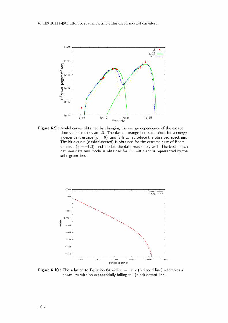
6. 1ES 1011+496: Effect of spatial particle diffusion on spectral curvature
1e-14
1e-13
1e-12
1e-11
1e-10
1e-09
1e+10 1e+15 1e+20 1e+25
E2 d
N/d
E [erg
s/c
m2/s
ec]
Freq [Hz]
s3ξ=0
ξ=-0.7ξ=-1.
Figure 6.9.: Model curves obtained by changing the energy dependence of the escapetime scale for the state s3. The dashed orange line is obtained for a energyindependent escape (ξ = 0), and fails to reproduce the observed spectrum.The blue curve (dashed-dotted) is obtained for the extreme case of Bohmdiffusion (ξ = −1.0), and models the data reasonably well. The best matchbetween data and model is obtained for ξ = −0.7 and is represented by thesolid green line.
1e-14
1e-12
1e-10
1e-08
1e-06
0.0001
0.01
1
100
10000
100 1000 10000 100000 1e+06 1e+07
dN
/dγ
Particle energy [γ]
ξ=-0.7CPL
Figure 6.10.: The solution to Equation 64 with ξ = −0.7 (red solid line) resembles apower law with an exponentially falling tail (black dotted line).
106
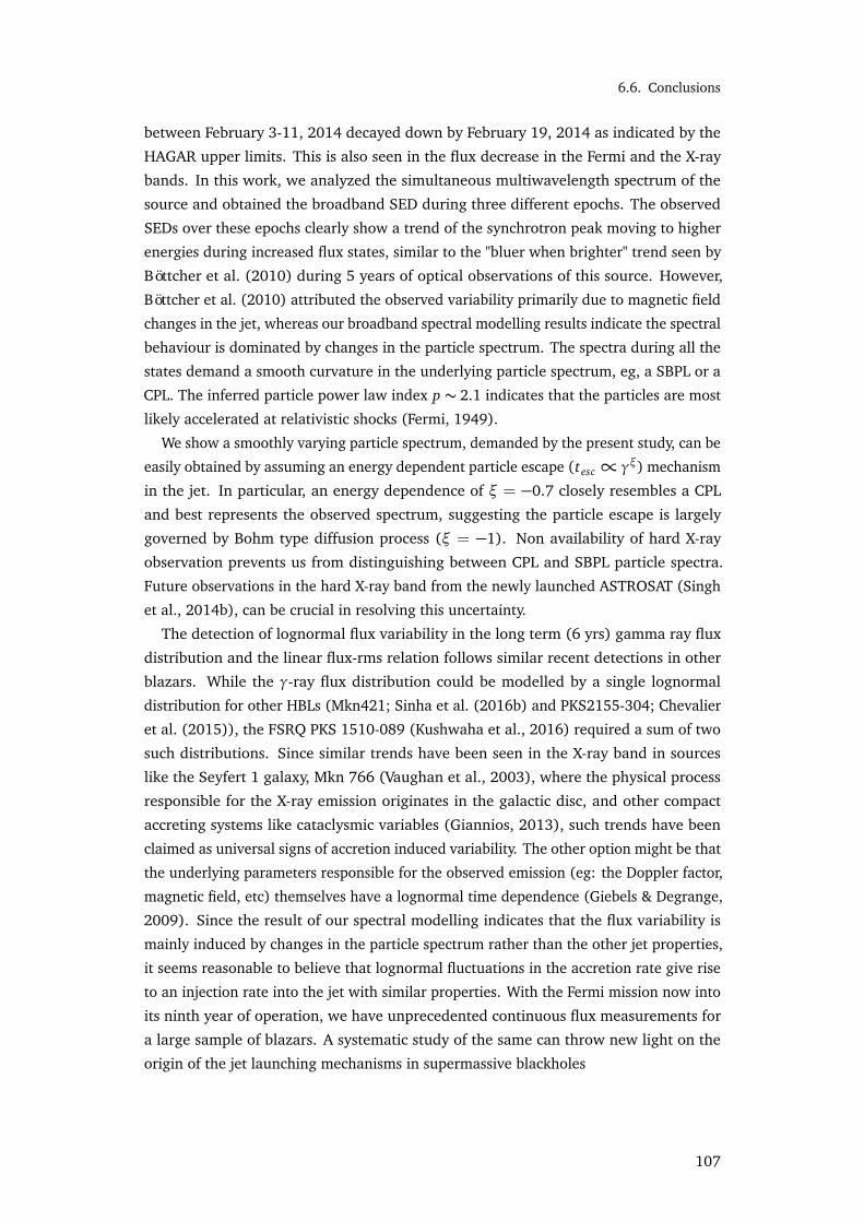
6.6. Conclusions
between February 3-11, 2014 decayed down by February 19, 2014 as indicated by the
HAGAR upper limits. This is also seen in the flux decrease in the Fermi and the X-ray
bands. In this work, we analyzed the simultaneous multiwavelength spectrum of the
source and obtained the broadband SED during three different epochs. The observed
SEDs over these epochs clearly show a trend of the synchrotron peak moving to higher
energies during increased flux states, similar to the "bluer when brighter" trend seen by
Böttcher et al. (2010) during 5 years of optical observations of this source. However,
Böttcher et al. (2010) attributed the observed variability primarily due to magnetic field
changes in the jet, whereas our broadband spectral modelling results indicate the spectral
behaviour is dominated by changes in the particle spectrum. The spectra during all the
states demand a smooth curvature in the underlying particle spectrum, eg, a SBPL or a
CPL. The inferred particle power law index p ∼ 2.1 indicates that the particles are most
likely accelerated at relativistic shocks (Fermi, 1949).
We show a smoothly varying particle spectrum, demanded by the present study, can be
easily obtained by assuming an energy dependent particle escape (tesc ∝ γξ) mechanism
in the jet. In particular, an energy dependence of ξ = −0.7 closely resembles a CPL
and best represents the observed spectrum, suggesting the particle escape is largely
governed by Bohm type diffusion process (ξ = −1). Non availability of hard X-ray
observation prevents us from distinguishing between CPL and SBPL particle spectra.
Future observations in the hard X-ray band from the newly launched ASTROSAT (Singh
et al., 2014b), can be crucial in resolving this uncertainty.
The detection of lognormal flux variability in the long term (6 yrs) gamma ray flux
distribution and the linear flux-rms relation follows similar recent detections in other
blazars. While the γ-ray flux distribution could be modelled by a single lognormal
distribution for other HBLs (Mkn421; Sinha et al. (2016b) and PKS2155-304; Chevalier
et al. (2015)), the FSRQ PKS 1510-089 (Kushwaha et al., 2016) required a sum of two
such distributions. Since similar trends have been seen in the X-ray band in sources
like the Seyfert 1 galaxy, Mkn 766 (Vaughan et al., 2003), where the physical process
responsible for the X-ray emission originates in the galactic disc, and other compact
accreting systems like cataclysmic variables (Giannios, 2013), such trends have been
claimed as universal signs of accretion induced variability. The other option might be that
the underlying parameters responsible for the observed emission (eg: the Doppler factor,
magnetic field, etc) themselves have a lognormal time dependence (Giebels & Degrange,
2009). Since the result of our spectral modelling indicates that the flux variability is
mainly induced by changes in the particle spectrum rather than the other jet properties,
it seems reasonable to believe that lognormal fluctuations in the accretion rate give rise
to an injection rate into the jet with similar properties. With the Fermi mission now into
its ninth year of operation, we have unprecedented continuous flux measurements for
a large sample of blazars. A systematic study of the same can throw new light on the
origin of the jet launching mechanisms in supermassive blackholes
107


“It is far better to grasp the universe as it really is than to
persist in delusion, however satisfying and reassuring."
Carl Sagan
7The Extragalactic Background Light:Estimation using TeV observations
THE UNIVERSE IS NOT AS DARK as we sometimes imagine; even its largest voids are
filled with light. While the total energy content of the universe in the electromagnetic
spectrum spans close to 20 decades in wavelength from γ-rays to radio (Figure 7.1),
the Extragalactic Background Light (EBL) is usually (and in this thesis) defined as
the extragalactic spectrum from Ultraviolet (UV) to Infrared (IR) wavelengths (λ =
0.1 − 1000µm) (Hauser & Dwek, 2001; Dwek & Krennrich, 2013). It is the second most
dominant background in the universe after the Cosmic Microwave Background (CMB). It
is the relic radiation containing information about the structure formation epoch of the
universe, and hence, an important cosmological quantity (Dwek & Krennrich, 2013; De
Angelis et al., 2013). Moreover, VHE photons from distant sources blazars are absorbed
en-route by forming electron-positron pairs on interaction with the photons of the EBL,
causing the observed spectrum to differ significantly from the intrinsic one. This makes
a proper understanding of the EBL crucial for VHE astrophysics.
In this chapter we discuss the challenges in direct measurements and theoretical
predictions of the EBL intensity. Novel techniques using the VHE blazar observations
have been proposed to indirectly constrain the EBL intensity, and we show how a statistical
study of TeV blazars can be used to obtain a model independent estimate of the EBL
(Sinha et al., 2014).
7.1 I N T R O D U C T I O N
The cosmological significance of the EBL was recognised almost immediately with the
advent of modern astronomy. It was first proposed in its mature form by the German
109
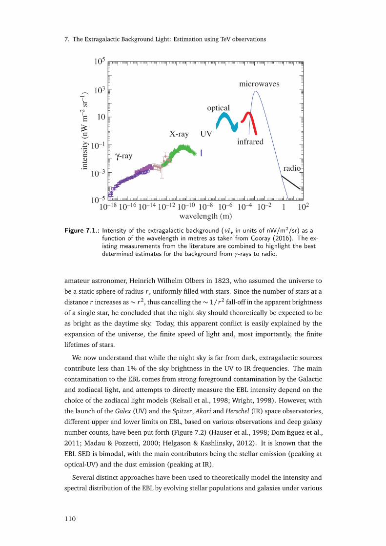
7. The Extragalactic Background Light: Estimation using TeV observations
Figure 7.1.: Intensity of the extragalactic background (νIν in units of nW/m2/sr) as afunction of the wavelength in metres as taken from Cooray (2016). The ex-isting measurements from the literature are combined to highlight the bestdetermined estimates for the background from γ-rays to radio.
amateur astronomer, Heinrich Wilhelm Olbers in 1823, who assumed the universe to
be a static sphere of radius r, uniformly filled with stars. Since the number of stars at a
distance r increases as∼ r2, thus cancelling the∼ 1/r2 fall-off in the apparent brightness
of a single star, he concluded that the night sky should theoretically be expected to be
as bright as the daytime sky. Today, this apparent conflict is easily explained by the
expansion of the universe, the finite speed of light and, most importantly, the finite
lifetimes of stars.
We now understand that while the night sky is far from dark, extragalactic sources
contribute less than 1% of the sky brightness in the UV to IR frequencies. The main
contamination to the EBL comes from strong foreground contamination by the Galactic
and zodiacal light, and attempts to directly measure the EBL intensity depend on the
choice of the zodiacal light models (Kelsall et al., 1998; Wright, 1998). However, with
the launch of the Galex (UV) and the Spitzer, Akari and Herschel (IR) space observatories,
different upper and lower limits on EBL, based on various observations and deep galaxy
number counts, have been put forth (Figure 7.2) (Hauser et al., 1998; Domínguez et al.,
2011; Madau & Pozzetti, 2000; Helgason & Kashlinsky, 2012). It is known that the
EBL SED is bimodal, with the main contributors being the stellar emission (peaking at
optical-UV) and the dust emission (peaking at IR).
Several distinct approaches have been used to theoretically model the intensity and
spectral distribution of the EBL by evolving stellar populations and galaxies under various
110
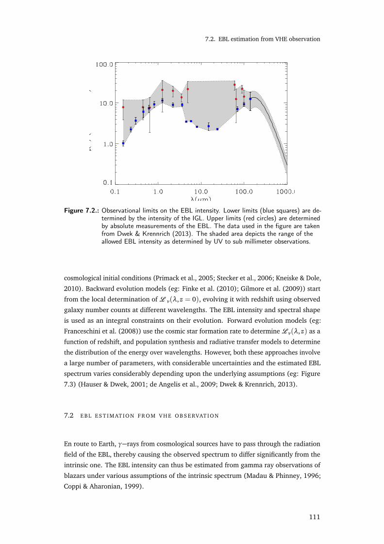
7.2. EBL estimation from VHE observation
Figure 7.2.: Observational limits on the EBL intensity. Lower limits (blue squares) are de-termined by the intensity of the IGL. Upper limits (red circles) are determinedby absolute measurements of the EBL. The data used in the figure are takenfrom Dwek & Krennrich (2013). The shaded area depicts the range of theallowed EBL intensity as determined by UV to sub millimeter observations.
cosmological initial conditions (Primack et al., 2005; Stecker et al., 2006; Kneiske & Dole,
2010). Backward evolution models (eg: Finke et al. (2010); Gilmore et al. (2009)) start
from the local determination of L ν(λ, z = 0), evolving it with redshift using observed
galaxy number counts at different wavelengths. The EBL intensity and spectral shape
is used as an integral constraints on their evolution. Forward evolution models (eg:
Franceschini et al. (2008)) use the cosmic star formation rate to determine Lν(λ, z) as a
function of redshift, and population synthesis and radiative transfer models to determine
the distribution of the energy over wavelengths. However, both these approaches involve
a large number of parameters, with considerable uncertainties and the estimated EBL
spectrum varies considerably depending upon the underlying assumptions (eg: Figure
7.3) (Hauser & Dwek, 2001; de Angelis et al., 2009; Dwek & Krennrich, 2013).
7.2 E B L E S T I M AT I O N F R O M V H E O B S E RVAT I O N
En route to Earth, γ−rays from cosmological sources have to pass through the radiation
field of the EBL, thereby causing the observed spectrum to differ significantly from the
intrinsic one. The EBL intensity can thus be estimated from gamma ray observations of
blazars under various assumptions of the intrinsic spectrum (Madau & Phinney, 1996;
Coppi & Aharonian, 1999).
111

7. The Extragalactic Background Light: Estimation using TeV observations
Figure 7.3.: Comparison of τ at z=0.5, taken from Mankuzhiyil (2010). The blue linecorresponds to the model of Gilmore (2009) Gilmore et al. (2009); red line toFranceschini (2008) Franceschini et al. (2008); green line to Kneiske Kneiske& Dole (2010); cyan line to Raue (2008) Raue & Mazin (2008); black line toStecker (2006) (solid line: fast evolution, dotted line: baseline fit).
7.2.1 Interaction of VHE photons with the EBL
A high energy photon of energy Eγinteracts with a low energy photon of energy εb,
leading to a creation of a particle anti-particle pair when the total γ−ray energy in the
center of momentum of the system exceeds the rest frame energy of the two particles.
The threshold for the creation of an e++e− pair is then given by:
εth(Eγ,µ, z) =2 (me c2)2
Eγ (1−µ)(65)
where µ ≡ cosθ , and θ is the angle between the two photons, as illustrated in Figure
7.4.
The cross-section for the γ−γ interaction is given by:
σγγ(Eγ,ε,µ, z) =3σT
16(1−β2)
2β (β2−2)+ (3−β4) ln
1+β)
(1−β)
(66)
where
β ≡s
1−εth
ε
(67)
7.2.2 EBL estimates computed from VHE observations
Though the broadband emission from blazars is not well understood, various constraints
on the EBL density have been derived under different assumptions of the intrinsic blazar
112

7.2. EBL estimation from VHE observation
θ
γ
γ
e
e+
.
Figure 7.4.: Schematic illustration of the γ−γ pair production reaction, showing the defini-tion of the angle θ between the interacting photons
Figure 7.5.: The cross section for the γ− γ interaction. Left panel: its dependence on β[eq. (7)] The cross section peaks at a value of β = 0.70; Right panel: itsdependence on b for different angles of incidence. When the photons aremoving in the same direction (θ = 0), the cross section collapses to a delta-function at b = 0, and the energy threshold becomes infinite.
113
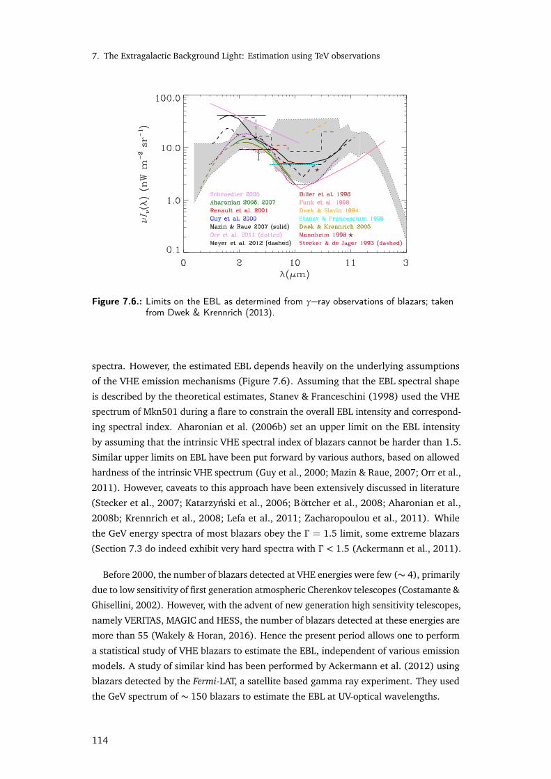
7. The Extragalactic Background Light: Estimation using TeV observations
Figure 7.6.: Limits on the EBL as determined from γ−ray observations of blazars; takenfrom Dwek & Krennrich (2013).
spectra. However, the estimated EBL depends heavily on the underlying assumptions
of the VHE emission mechanisms (Figure 7.6). Assuming that the EBL spectral shape
is described by the theoretical estimates, Stanev & Franceschini (1998) used the VHE
spectrum of Mkn501 during a flare to constrain the overall EBL intensity and correspond-
ing spectral index. Aharonian et al. (2006b) set an upper limit on the EBL intensity
by assuming that the intrinsic VHE spectral index of blazars cannot be harder than 1.5.
Similar upper limits on EBL have been put forward by various authors, based on allowed
hardness of the intrinsic VHE spectrum (Guy et al., 2000; Mazin & Raue, 2007; Orr et al.,
2011). However, caveats to this approach have been extensively discussed in literature
(Stecker et al., 2007; Katarzynski et al., 2006; Böttcher et al., 2008; Aharonian et al.,
2008b; Krennrich et al., 2008; Lefa et al., 2011; Zacharopoulou et al., 2011). While
the GeV energy spectra of most blazars obey the Γ = 1.5 limit, some extreme blazars
(Section 7.3 do indeed exhibit very hard spectra with Γ < 1.5 (Ackermann et al., 2011).
Before 2000, the number of blazars detected at VHE energies were few (∼ 4), primarily
due to low sensitivity of first generation atmospheric Cherenkov telescopes (Costamante &
Ghisellini, 2002). However, with the advent of new generation high sensitivity telescopes,
namely VERITAS, MAGIC and HESS, the number of blazars detected at these energies are
more than 55 (Wakely & Horan, 2016). Hence the present period allows one to perform
a statistical study of VHE blazars to estimate the EBL, independent of various emission
models. A study of similar kind has been performed by Ackermann et al. (2012) using
blazars detected by the Fermi-LAT, a satellite based gamma ray experiment. They used
the GeV spectrum of ∼ 150 blazars to estimate the EBL at UV-optical wavelengths.
114
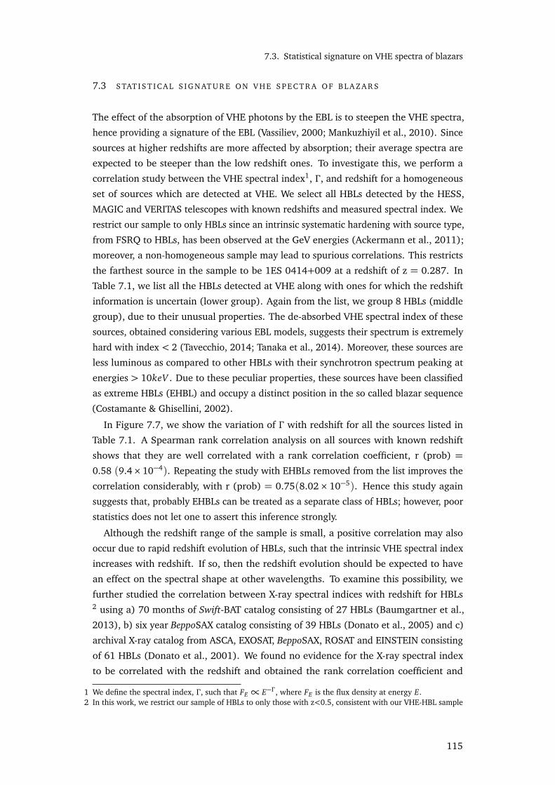
7.3. Statistical signature on VHE spectra of blazars
7.3 S TAT I S T I CA L S I G N AT U R E O N V H E S P E C T R A O F B L A Z A R S
The effect of the absorption of VHE photons by the EBL is to steepen the VHE spectra,
hence providing a signature of the EBL (Vassiliev, 2000; Mankuzhiyil et al., 2010). Since
sources at higher redshifts are more affected by absorption; their average spectra are
expected to be steeper than the low redshift ones. To investigate this, we perform a
correlation study between the VHE spectral index1, Γ , and redshift for a homogeneous
set of sources which are detected at VHE. We select all HBLs detected by the HESS,
MAGIC and VERITAS telescopes with known redshifts and measured spectral index. We
restrict our sample to only HBLs since an intrinsic systematic hardening with source type,
from FSRQ to HBLs, has been observed at the GeV energies (Ackermann et al., 2011);
moreover, a non-homogeneous sample may lead to spurious correlations. This restricts
the farthest source in the sample to be 1ES 0414+009 at a redshift of z = 0.287. In
Table 7.1, we list all the HBLs detected at VHE along with ones for which the redshift
information is uncertain (lower group). Again from the list, we group 8 HBLs (middle
group), due to their unusual properties. The de-absorbed VHE spectral index of these
sources, obtained considering various EBL models, suggests their spectrum is extremely
hard with index < 2 (Tavecchio, 2014; Tanaka et al., 2014). Moreover, these sources are
less luminous as compared to other HBLs with their synchrotron spectrum peaking at
energies > 10keV . Due to these peculiar properties, these sources have been classified
as extreme HBLs (EHBL) and occupy a distinct position in the so called blazar sequence
(Costamante & Ghisellini, 2002).
In Figure 7.7, we show the variation of Γ with redshift for all the sources listed in
Table 7.1. A Spearman rank correlation analysis on all sources with known redshift
shows that they are well correlated with a rank correlation coefficient, r (prob) =
0.58 (9.4×10⁻⁴). Repeating the study with EHBLs removed from the list improves the
correlation considerably, with r (prob) = 0.75(8.02× 10⁻⁵). Hence this study again
suggests that, probably EHBLs can be treated as a separate class of HBLs; however, poor
statistics does not let one to assert this inference strongly.
Although the redshift range of the sample is small, a positive correlation may also
occur due to rapid redshift evolution of HBLs, such that the intrinsic VHE spectral index
increases with redshift. If so, then the redshift evolution should be expected to have
an effect on the spectral shape at other wavelengths. To examine this possibility, we
further studied the correlation between X-ray spectral indices with redshift for HBLs2 using a) 70 months of Swift-BAT catalog consisting of 27 HBLs (Baumgartner et al.,
2013), b) six year BeppoSAX catalog consisting of 39 HBLs (Donato et al., 2005) and c)
archival X-ray catalog from ASCA, EXOSAT, BeppoSAX, ROSAT and EINSTEIN consisting
of 61 HBLs (Donato et al., 2001). We found no evidence for the X-ray spectral index
to be correlated with the redshift and obtained the rank correlation coefficient and
1 We define the spectral index, Γ , such that FE ∝ E−Γ , where FE is the flux density at energy E.2 In this work, we restrict our sample of HBLs to only those with z<0.5, consistent with our VHE-HBL sample
115

7. The Extragalactic Background Light: Estimation using TeV observations
Source name z Γ EV HE α2 α f RefMkn421 0.031 2.72 ± 0.12 0.2 - 10 2.58 ± 0.03 1.771 ± 0.012 1Mkn501 0.034 2.79 ± 0.12 0.1 - 2.0 2.42 ± 0.01 1.738 ± 0.027 21ES 2344+514∗ 0.044 2.95 ± 0.20 0.2 - 2.0 2.62 ± 0.50 1.716 ± 0.08 3Mkn180 0.045 3.30 ± 0.70 0.2 - 6.6 - 1.74 ± 0.083 41ES 1959+650 0.048 2.58 ± 0.18 0.2 - 2.5 2.19 ± 0.02 1.937 ± 0.031 51ES 1727+502 0.055 2.70 ± 0.50 0.15 - 2.0 - 2.0 ± 0.2 6PKS 0548−322∗ 0.069 2.86 ± 0.34 0.3 - 4.0 2.28 ± 0.23 - 7PKS 2005−489 0.071 3.00 ± 0.22 0.4 - 4.0 2.46 ± 0.01 1.779 ± 0.047 8RGB J0152+017 0.080 2.95 ± 0.36 0.1 - 4.0 - 1.788 ± 0.137 9BZB J0013-1854 0.095 3.4 ± 0.10 0.2 - 2.0 - 1.96 ± 0.2 101ES 1312-423 0.105 2.85 ± 0.7 0.2 - 4.0 - 1.4 ± 0.4 11PKS 2155−304 0.116 3.34 ± 0.10 1.0 - 10. 2.36 ± 0.01 1.838 ± 0.015 12B3 2247+381 0.119 3.20 ± 0.60 0.1 - 2.0 - 1.837 ± 0.113 13H 1426+428∗ 0.129 3.50 ± 0.40 0.3 - 2.00 2.54 ± 0.24 1.316 ± 0.123 141ES 1215+304 0.130 2.96 ± 0.14 0.1 - 1.51 2.29 ± 0.16 2.019 ± 0.036 151ES 0806+524 0.138 3.60 ± 1.00 0.3 - 1.02 2.67 ± 0.08 1.938 ± 0.057 16BZB J1010−3119 0.143 3.08 ± 0.42 0.25 - 3.0 2.15 ± 0.06 2.239 ± 0.142 17RX J0648+1516 0.179 4.40 ± 0.80 0.2 - 0.65 2.51 ± 0.06 1.737 ± 0.106 18RBS 0413 0.190 3.18 ± 0.68 0.3 - 1.0 2.22 ± 0.07 1.551 ± 0.112 191ES 1011+496 0.212 4.00 ± 0.50 0.15 - 0.8 - - 20PKS 0301−243 0.266 4.60 ± 0.70 0.1 - 5 2.51 ± 0.1 1.938 ± 0.031 21
IC310 0.019 1.96 ± 0.22 0.12 - 8.1 - 22RGB J0710+591∗ 0.125 2.69 ± 0.22 0.3 - 7.9 2.29 ± 0.26 231ES0229+200 0.140 2.50 ± 0.19 0.5 - 15.0 2.16 ± 0.28 24H 2356-309 0.165 3.09 ± 0.24 0.2 - 1.04 2.43 ± 0.11 251ES 1218+304 0.182 3.08 ± 0.40 0.1 - 2 - 261ES 1101−232 0.186 2.94 ± 0.20 0.1 - 0.66 2.32 ± 0.02 271ES 0347−121∗ 0.188 3.10 ± 0.23 0.3 - 3 2.27 ± 0.30 281ES 0414+009 0.287 3.40 ± 0.50 0.2 - 0.70 2.40 ± 0.10 29
HESS J1943+213 0.14 3.1 ± 0.30 301ES 1440+122 0.163 3.4 ± 0.7 31PKS 0447-439 0.175 3.8 ± 0.4 321ES 0502+675 0.341 3.9 ± 0.4 33PG 1553+113 0.5 ± 0.08 4.1 ± 0.3 34PKS 1424+240 0.604 4.2 ± 0.7 35
Table 7.1.: The list of HBLs detected at VHE. The middle group lists the extreme HBLsand the bottom one with uncertain redshift. Column description 1: the Sourcename, 2: the redshift (z), 3: Observed VHE spectral index (Γ ), 4: ObservedVHE energy range (in TeV), 5: X-ray Spectral Index (quantities with * areobtained from Swift-BAT) 6. The Fermi-LAT average index, and 7: References:1. Aleksić et al. (2012b) 2. Anderhub et al. (2009b) 3. Albert et al. (2007c)4. Albert et al. (2006) 5. Tagliaferri et al. (2008) 6. Aleksić et al. (2014b) 7.Aharonian et al. (2010) 8. H.E.S.S. Collaboration et al. (2011) 9. Aharonianet al. (2008a) 10. H.E.S.S. Collaboration et al. (2013b) 11. HESS Collab-oration et al. (2013) 12. Aharonian et al. (2009) 13. Aleksić et al. (2012c)14 .Petry et al. (2002) 15.Aleksić et al. (2012a) 16.Acciari et al. (2009a)17. H.E.S.S. Collaboration et al. (2012) 18. Aliu et al. (2011) 19. Aliu et al.(2012a) 20. Albert et al. (2007b) 21. H.E.S.S. Collaboration et al. (2013a) 22.Aleksić et al. (2014c) 23. Acciari et al. (2010) 24. Aharonian et al. (2007a) 25.Aharonian et al. (2006a) 26. Acciari et al. (2009b) 27. Reimer et al. (2008)28. Aharonian et al. (2007b) 29.Aliu et al. (2012b) 30 - 35. www.tevcat.edu
116
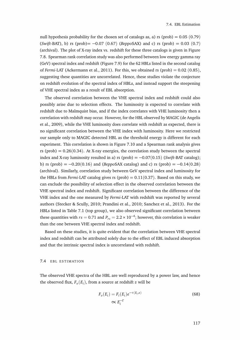
7.4. EBL Estimation
null hypothesis probability for the chosen set of catalogs as, a) rs (prob) = 0.05 (0.79)
(Swift-BAT), b) rs (prob)= −0.07 (0.67) (BeppoSAX) and c) rs (prob) = 0.03 (0.7)
(archival). The plot of X-ray index vs. redshift for these three catalogs is given in Figure
7.8. Spearman rank correlation study was also performed between low energy gamma ray
(GeV) spectral index and redshift (Figure 7.9) for the 62 HBLs listed in the second catalog
of Fermi-LAT (Ackermann et al., 2011). For this, we obtained rs (prob) = 0.02 (0.85),
suggesting these quantities are uncorrelated. Hence, these studies violate the conjecture
on redshift evolution of the spectral index of HBLs, and instead support the steepening
of VHE spectral index as a result of EBL absorption.
The observed correlation between the VHE spectral index and redshift could also
possibly arise due to selection effects. The luminosity is expected to correlate with
redshift due to Malmquist bias, and if the index correlates with VHE luminosity then a
correlation with redshift may occur. However, for the HBL observed by MAGIC (de Angelis
et al., 2009), while the VHE luminosity does correlate with redshift as expected, there is
no significant correlation between the VHE index with luminosity. Here we restricted
our sample only to MAGIC detected HBL as the threshold energy is different for each
experiment. This correlation is shown in Figure 7.10 and a Spearman rank analysis gives
rs (prob) = 0.26(0.34). At X-ray energies, the correlation study between the spectral
index and X-ray luminosity resulted in a) rs (prob) = −0.07(0.15) (Swift-BAT catalog);
b) rs (prob) = −0.20(0.16) and (BeppoSAX catalog) and c) rs (prob) = −0.14(0.28)
(archival). Similarly, correlation study between GeV spectral index and luminosity for
the HBLs from Fermi-LAT catalog gives rs (prob) = 0.11(0.37). Based on this study, we
can exclude the possibility of selection effect in the observed correlation between the
VHE spectral index and redshift. Significant correlation between the difference of the
VHE index and the one measured by Fermi-LAT with redshift was reported by several
authors (Stecker & Scully, 2010; Prandini et al., 2010; Sanchez et al., 2013). For the
HBLs listed in Table 7.1 (top group), we also observed significant correlation between
these quantities with rs = 0.71 and Prs = 2.2×10⁻⁴; however, this correlation is weaker
than the one between VHE spectral index and redshift.
Based on these studies, it is quite evident that the correlation between VHE spectral
index and redshift can be attributed solely due to the effect of EBL induced absorption
and that the intrinsic spectral index is uncorrelated with redshift.
7.4 E B L E S T I M AT I O N
The observed VHE spectra of the HBL are well reproduced by a power law, and hence
the observed flux, Fo(Ei), from a source at redshift z will be
Fo(Ei) = Fi(Ei)e−τ(Ei ,z) (68)
∝ E−Γi
117
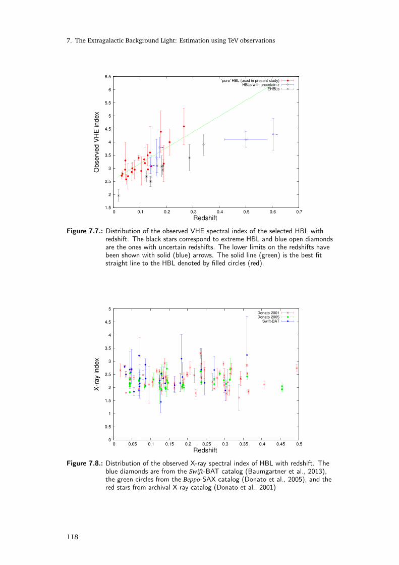
7. The Extragalactic Background Light: Estimation using TeV observations
1.5
2
2.5
3
3.5
4
4.5
5
5.5
6
6.5
0 0.1 0.2 0.3 0.4 0.5 0.6 0.7
Observ
ed V
HE
index
Redshift
’pure’ HBL (used in present study)HBLs with uncertain z
EHBLs
Figure 7.7.: Distribution of the observed VHE spectral index of the selected HBL withredshift. The black stars correspond to extreme HBL and blue open diamondsare the ones with uncertain redshifts. The lower limits on the redshifts havebeen shown with solid (blue) arrows. The solid line (green) is the best fitstraight line to the HBL denoted by filled circles (red).
0
0.5
1
1.5
2
2.5
3
3.5
4
4.5
5
0 0.05 0.1 0.15 0.2 0.25 0.3 0.35 0.4 0.45 0.5
X-r
ay index
Redshift
Donato 2001Donato 2005
Swift-BAT
Figure 7.8.: Distribution of the observed X-ray spectral index of HBL with redshift. Theblue diamonds are from the Swift-BAT catalog (Baumgartner et al., 2013),the green circles from the Beppo-SAX catalog (Donato et al., 2005), and thered stars from archival X-ray catalog (Donato et al., 2001)
118
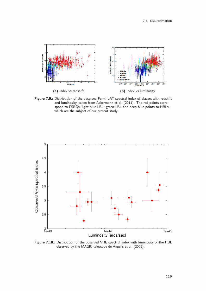
7.4. EBL Estimation
(a) Index vs redshift (b) Index vs luminosity
Figure 7.9.: Distribution of the observed Fermi-LAT spectral index of blazars with redshiftand luminosity, taken from Ackermann et al. (2011). The red points corre-spond to FSRQs, light blue LBL, green LBL and deep blue points to HBLs,which are the subject of our present study.
2
2.5
3
3.5
4
4.5
5
1e+43 1e+44 1e+45
Observ
ed V
HE
spectr
al in
dex
Luminosity [ergs/sec]
Figure 7.10.: Distribution of the observed VHE spectral index with luminosity of the HBLobserved by the MAGIC telescope de Angelis et al. (2009).
119
7. The Extragalactic Background Light: Estimation using TeV observations
where Fi(Ei) is the de-absorbed flux at energy Ei and τ, the optical depth due to EBL
absorption given by (Gould & Schréder, 1967)
τ(Ei , z) =
z∫
0
dz′dldz′
1∫
−1
dµ(1−µ)
2
∞∫
εth
dεz′n(εz′ , z′)σγγ(Ei ,εz′ ,µ) (69)
Here,dldz′
=c
H0
1
(1+ z′)Æ
ΩΛ+ΩM (1+ z′)3, (70)
is the distance traveled by a photon per unit redshift with c as the velocity of light,
n is the number density of the EBL photon of energy εz′[= ε0(1+ z′)] at redshift z′,
corresponding to a photon energy ε0 at z = 0, εth [= 2m2e c4 (1+ z′)/(Ei(1−µ))] is
the threshold soft photon energy with µ the cosine of the interaction angle and the pair
production cross section, σγγ, is given by
σγγ(E,ε,µ) =2πα2
3m2e(1−β2)×
2β(β2−2)+ (3−β4) ln
1+β1−β
(71)
with β(E,ε) =Æ
1− (2 m2e c4)/(ε E (1−µ)) being the speed of the electron/positron
in the centre of mass frame, α is the fine structure constant and me is the electron rest
mass. Since VHE sources are detected only at low redshifts, one can neglect the evolution
of EBL and hence (Madau & Phinney, 1996),
n(εz , z) ≈ (1+ z)3n(εz) (72)
For an isotropic EBL distribution, the angle integrated cross section (Gould & Schréder,
1967)
σγγ(Eε) =12
1∫
−1
dµ(1−µ)σγγ(E,ε,µ) (73)
peaks at Eε = 3.56 m2e c4. Approximating σγγ as a delta function along with Ez ≈ Ei
and εz ≈ ε0, equation (69) can be simplified to
τ(E, z) ≈ Aγγ εn(ε) f (z) (74)
where Aγγ(≈ 3.7×10⁻²⁶ cm2) is a constant, ε≈ 3.6 m2e c4
E and f (z) is given by
f (z) =
z∫
0
dz′dldz′
(1+ z′)3 (75)
≈c
H0z
120
7.4. EBL Estimation
If the source spectrum is assumed to be a power-law, Fi(E)∝ E−ζ, then using equations
(68) and (74) we obtain
εn(ε) = k ln εp
ε
(76)
where k = Γ−ζAγγ f (z) and εp ≈
3.56 m2e c4
E? are source independent constants with E? being the
energy of the gamma ray photon at which the EBL induced absorption is negligible. While
this form of the EBL spectrum is derived for the approximate optical depth equation (74),
we have verified numerically that for the range of redshifts considered here, this EBL
spectral shape will result in a nearly power-law observed spectrum. In particular, we have
verified that if the EBL spectra is defined by equation (76) and the absorption optical
depth is given by equation (69), the observed VHE spectrum for a source at z = 0.3
can be well described as a power-law. The deviation from a power-law for sources with
z < 0.3 is less than 10 %. Hence for all calculations in this work we have used equation
(69) for the optical depth. It may be noted that Stecker & Scully (2006) obtained a
similar form of the optical depth while approximating a theoretical EBL spectrum by an
analytic expression. However, here we arrive at this form of the EBL spectrum equation
(76) only from the criterion that both the intrinsic and absorbed VHE spectra are well
described by a power-law and hence our approach is independent of any cosmological
calculations.
The EBL spectrum given by equation (76) is characterized by two constants, namely k
and εp, which in turn determines the source spectral index. Since the source spectral
index should be uncorrelated with redshift (Section 7.3), the allowed range of k and
εp is restricted. For k = 2.4×10⁻³cm−3 and εp = 4.6 eV, we found that the computed
source spectral indices, for the sources listed in Table 7.1 (top group), turn out to
be “most” uncorrelated with rs = 0.001 and a maximum null hypothesis probability
Prs = 0.99. Within 1−σ confidence limit, corresponding to Prs > 0.33, we obtained the
range of k and εp as 2.2+1.6−0.7 ×10⁻³ cm−3 and 4.6+4.4
−3.4 eV , respectively. The resultant EBL
spectrum, consistent with these values of k and εp, is plotted in Figure 7.11 along with
the constraints derived from various observations (Dwek & Krennrich, 2013) and other
theoretical estimates (Gilmore et al., 2009; Franceschini et al., 2008; Finke et al., 2010;
Kneiske & Dole, 2010). If we consider all the HBL with known redshift in Table 7.1 (top
and middle group), the 1−σ confidence limit of k and εp are 2.8+2.6−1.8 ×10⁻³ cm−3 and
5.2+4.8−4.0 eV , respectively.
Alternatively, a linear fit over source spectral index versus redshift can be used to
constrain the constants k and εp. A linear fit between Γ and redshift resulted in a straight
line of slope 6.0±1.1 with reduced chi-square χ2red ≈ 1.1. Since the source spectral index
is uncorrelated with the redshift (§7.3), a linear fit between these quantities should result
in a constant line (a line with slope 0). Within 1-σ confidence limit, this corresponds
to an EBL spectrum with k = 2.4+1.2−0.8 ×10⁻³ cm−3 and εp = 5.2+3.8
−4.0 eV , for which this
condition can be achieved. We find that these constraints on k and εp are consistent with
121
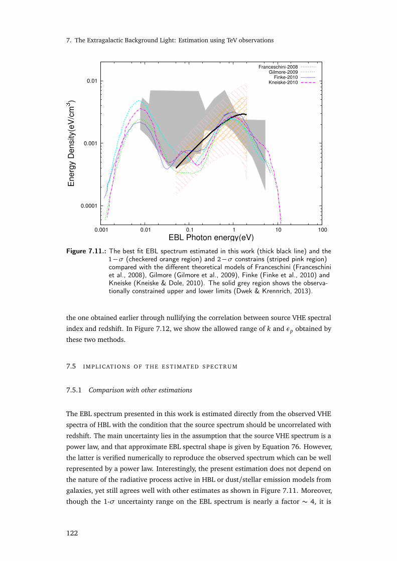
7. The Extragalactic Background Light: Estimation using TeV observations
En
erg
y D
en
sity(e
V/c
m3)
EBL Photon energy(eV)
Franceschini-2008Gilmore-2009
Finke-2010Kneiske-2010
0.0001
0.001
0.01
0.001 0.01 0.1 1 10 100
Figure 7.11.: The best fit EBL spectrum estimated in this work (thick black line) and the1−σ (checkered orange region) and 2−σ constrains (striped pink region)compared with the different theoretical models of Franceschini (Franceschiniet al., 2008), Gilmore (Gilmore et al., 2009), Finke (Finke et al., 2010) andKneiske (Kneiske & Dole, 2010). The solid grey region shows the observa-tionally constrained upper and lower limits (Dwek & Krennrich, 2013).
the one obtained earlier through nullifying the correlation between source VHE spectral
index and redshift. In Figure 7.12, we show the allowed range of k and εp obtained by
these two methods.
7.5 I M P L I CAT I O N S O F T H E E S T I M AT E D S P E C T R U M
7.5.1 Comparison with other estimations
The EBL spectrum presented in this work is estimated directly from the observed VHE
spectra of HBL with the condition that the source spectrum should be uncorrelated with
redshift. The main uncertainty lies in the assumption that the source VHE spectrum is a
power law, and that approximate EBL spectral shape is given by Equation 76. However,
the latter is verified numerically to reproduce the observed spectrum which can be well
represented by a power law. Interestingly, the present estimation does not depend on
the nature of the radiative process active in HBL or dust/stellar emission models from
galaxies, yet still agrees well with other estimates as shown in Figure 7.11. Moreover,
though the 1-σ uncertainty range on the EBL spectrum is nearly a factor ∼ 4, it is
122

7.5. Implications of the estimated spectrum
0
1
2
3
4
5
6
7
8
9
10
0.001 0.0015 0.002 0.0025 0.003 0.0035 0.004
εp
k [1/cm3]
st line fitcorrelation
Figure 7.12.: The 1−σ confidence region for the parameters k and εp obtained fromthe correlation study (green forward stripes) and the straight line fit (redbackward stripes)
competitive compared to constraints put by observations and by other estimates. The
predicted EBL spectrum is reasonably confined within the upper and lower limits (grey
shaded area in Figure 7.11), obtained independently through observations (see §1).
When compared with the other EBL estimates, obtained through cosmological evolution
models, the present one predicts stronger emission at lower energies but closely agrees
at higher energies, though the predicted spectrum is not well constrained in this regime.
Deviation of the source spectrum from a power law may modify the EBL spectral
shape described by Equation 76 considerably. In such case, the present formalism needs
to be modified by studying the correlation of other suitable observables instead of the
power law spectral indices. However, the source spectrum of HBL (z<0.3) obtained
using various EBL models are fitted resonably well by a power law and the one presented
here agrees closely with these EBL models. To investigate further, we repeat the study
considering the EBL spectral shape due to Franceschini et al. (2008), Gilmore et al.
(2009), Finke et al. (2010) and Kneiske & Dole (2010). Following Abdo et al. (2010c);
Ackermann et al. (2012); H.E.S.S. Collaboration et al. (2013); Reesman & Walker (2013),
we define the observed spectrum to be
Fo(E) = Fi(Ez)ex p(−τtheor y(Ez , z)× b) (77)
123
7. The Extragalactic Background Light: Estimation using TeV observations
where τtheor y is the optical depth predicted by the above mentioned theoretical models,
and b is a normalization factor required to assure that the de-absorbed spectral index is
uncorrelated with the redshift. Then, b = 1.0 would imply that the particular model is
consistent with the non correlation of the source VHE index with redshift. For the models
discussed above, we obtained bKneisnke = 1.5−0.6+0.7, bF ranschini = 1.4−0.6
+0.7, bF inke = 1.1−0.5+0.6
and bGilmore = 1.6−0.5+0.7. From these, one can argue that the EBL model due to Finke et al.
(2010) well supports the non correlation of the source VHE index with redshift; whereas,
the deviation from this condition is observed to be maximum in case of Gilmore et al.
(2009).
The work presented here is similar to the EBL upper limits proposed by Schroedter
(2005) and Finke & Razzaque (2009). They studied the steepening of VHE spectral
index with increase in redshift and attributed it to the absorption by EBL. Schroedter
(2005) suggested an upper limit on EBL by assuming that the source spectral index, ζ,
cannot be harder than 1.8, whereas Finke & Razzaque (2009) considered limits for ζ as
1 and 1.5. Following a similar procedure, Yang & Wang (2010) proposed an EBL upper
limit by considering Fermi-LAT spectral index as an allowed limit on ζ. In this work, we
systematically study the steepening of the VHE spectra of HBL with respect to redshift
and exploit it to estimate the EBL spectrum. In addition, we do not impose any limits
on ζ; instead, the derived value of ζ, using the current EBL, lies well within our present
understanding of blazar emission models (Section 7.5.2).
Lately, various EBL estimates have been proposed, exploiting the properties of TeV
blazars under unique techniques. Mazin & Raue (2007) and Meyer et al. (2012) estimated
an upper limit on EBL by employing splines. From the observed VHE spectra of blazars,
they converged to a particular shape of EBL, which leads to a de-absorbed spectra that
are physically acceptable under the present understanding of blazars. Mankuzhiyil et al.
(2010); Domínguez et al. (2013) and Singh et al. (2014a) reproduced the broadband SED
of VHE blazars under leptonic model and thereby predicting the intrinsic VHE spectra.
Comparing this with the observed VHE spectra, they estimated the optical depth for the
attenuation of VHE gamma rays. While Mankuzhiyil et al. (2010) used this to show the
inconsistency among various EBL models interpreted theoretically, Singh et al. (2014a)
showed a systematic deviation of the optical depths towards high energy; between the
estimated and the ones predicted by various EBL models. Domínguez et al. (2013) used
the estimated optical depths to determine the cosmic gamma ray horizon. Reesman &
Walker (2013) considered the EBL models by Franceschini et al. (2008); Gilmore et al.
(2009); Domínguez et al. (2011) to estimate the optical depth for the VHE sources at
z ∼ 0.1. The optical depth is then scaled by a parameter to reproduce the observed
flux for a range of de-absorbed spectral indices. Based on this scaling parameter, they
concluded that these EBL models are consistent with the observed spectra, though the
error on the parameter is large. Unlike these models, the work presented here does not
have any bias on blazar emission models or a particular EBL shape. Instead, it relies
124
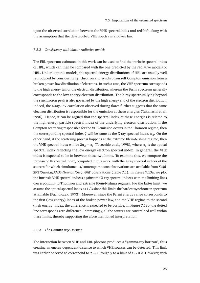
7.5. Implications of the estimated spectrum
upon the observed correlation between the VHE spectral index and redshift, along with
the assumption that the de-absorbed VHE spectra is a power law.
7.5.2 Consistency with blazar radiative models
The EBL spectrum estimated in this work can be used to find the intrinsic spectral index
of HBL, which can then be compared with the one predicted by the radiative models of
HBL. Under leptonic models, the spectral energy distributions of HBL are usually well
reproduced by considering synchrotron and synchrotron self Compton emission from a
broken power-law distribution of electrons. In such a case, the VHE spectrum corresponds
to the high energy tail of the electron distribution, whereas the Fermi spectrum generally
corresponds to the low energy electron distribution. The X-ray spectrum lying beyond
the synchrotron peak is also governed by the high energy end of the electron distribution.
Indeed, the X-ray-TeV correlation observed during flares further suggests that the same
electron distribution is responsible for the emission at these energies (Takahashi et al.,
1996). Hence, it can be argued that the spectral index at these energies is related to
the high energy particle spectral index of the underlying electron distribution. If the
Compton scattering responsible for the VHE emission occurs in the Thomson regime, then
the corresponding spectral index ζ will be same as the X-ray spectral index, α2. On the
other hand, if the scattering process happens at the extreme Klein-Nishina regime, then
the VHE spectral index will be 2α2−α1 (Tavecchio et al., 1998), where α1 is the optical
spectral index reflecting the low energy electron spectral index. In general, the VHE
index is expected to lie in between these two limits. To examine this, we compare the
intrinsic VHE spectral index, computed in this work, with the X-ray spectral indices of the
sources for which simultaneous/contemporaneous observations are available from Swift-
XRT/Suzaku/XMM-Newton/Swift-BAT observations (Table 7.1). In Figure 7.13a, we plot
the intrinsic VHE spectral indices against the X-ray spectral indices with the limiting lines
corresponding to Thomson and extreme Klein-Nishina regimes. For the latter limit, we
assume the optical spectral index as 1/3 since this limits the hardest synchrotron spectrum
attainable (Pacholczyk, 1973). Moreover, since the Fermi energy range corresponds to
the first (low energy) index of the broken power law, and the VHE regime to the second
(high energy) index, the difference is expected to be positive. In Figure 7.13b, the dotted
line corresponds zero difference. Interestingly, all the sources are constrained well within
these limits, thereby supporting the afore mentioned interpretation.
7.5.3 The Gamma Ray Horizon
The interaction between VHE and EBL photons produces a “gamma-ray horizon", thus
creating an energy dependent distance to which VHE sources can be detected. This limit
was earlier believed to correspond to τ∼ 1, roughly to a limit of z ∼ 0.2. However, with
125
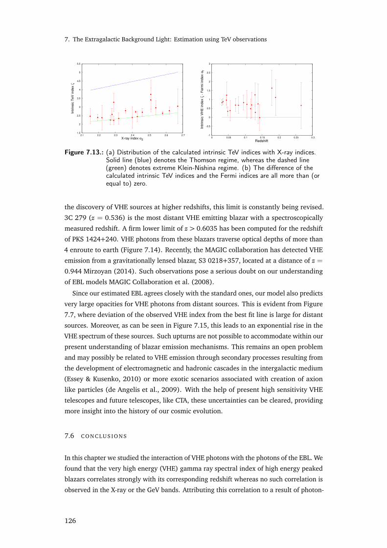
7. The Extragalactic Background Light: Estimation using TeV observations
1.5
2
2.5
3
3.5
4
4.5
5
5.5
2.1 2.2 2.3 2.4 2.5 2.6 2.7
Intr
insic
TeV
index ζ
X-ray index α2
-1
-0.5
0
0.5
1
1.5
2
2.5
3
0 0.05 0.1 0.15 0.2 0.25 0.3
Intr
insic
VH
E index ζ
- F
erm
i in
dex α
f
Redshift
Figure 7.13.: (a) Distribution of the calculated intrinsic TeV indices with X-ray indices.Solid line (blue) denotes the Thomson regime, whereas the dashed line(green) denotes extreme Klein-Nishina regime. (b) The difference of thecalculated intrinsic TeV indices and the Fermi indices are all more than (orequal to) zero.
the discovery of VHE sources at higher redshifts, this limit is constantly being revised.
3C 279 (z = 0.536) is the most distant VHE emitting blazar with a spectroscopically
measured redshift. A firm lower limit of z > 0.6035 has been computed for the redshift
of PKS 1424+240. VHE photons from these blazars traverse optical depths of more than
4 enroute to earth (Figure 7.14). Recently, the MAGIC collaboration has detected VHE
emission from a gravitationally lensed blazar, S3 0218+357, located at a distance of z =
0.944 Mirzoyan (2014). Such observations pose a serious doubt on our understanding
of EBL models MAGIC Collaboration et al. (2008).
Since our estimated EBL agrees closely with the standard ones, our model also predicts
very large opacities for VHE photons from distant sources. This is evident from Figure
7.7, where deviation of the observed VHE index from the best fit line is large for distant
sources. Moreover, as can be seen in Figure 7.15, this leads to an exponential rise in the
VHE spectrum of these sources. Such upturns are not possible to accommodate within our
present understanding of blazar emission mechanisms. This remains an open problem
and may possibly be related to VHE emission through secondary processes resulting from
the development of electromagnetic and hadronic cascades in the intergalactic medium
(Essey & Kusenko, 2010) or more exotic scenarios associated with creation of axion
like particles (de Angelis et al., 2009). With the help of present high sensitivity VHE
telescopes and future telescopes, like CTA, these uncertainties can be cleared, providing
more insight into the history of our cosmic evolution.
7.6 C O N C LU S I O N S
In this chapter we studied the interaction of VHE photons with the photons of the EBL. We
found that the very high energy (VHE) gamma ray spectral index of high energy peaked
blazars correlates strongly with its corresponding redshift whereas no such correlation is
observed in the X-ray or the GeV bands. Attributing this correlation to a result of photon-
126
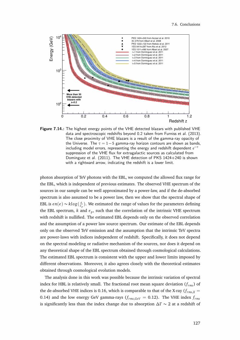
7.6. Conclusions
Redshift z
0 0.2 0.4 0.6 0.8 1 1.2
En
erg
y (
Ge
V)
210
310
410
More than 30
VHEdetected
blazars with
z<0.2
PKS 1424+240 from Acciari et al. 2010
3C 279 from Albert et al. 2008
PKS 1222+122 from Aleksic et al. 2011
1ES 0414+287 from Aliu et al. 2012
1ES 1011+496 from Albert et al. 2007=1 from Dominguez et al. 2011τ
=2 from Dominguez et al. 2011τ
=3 from Dominguez et al. 2011τ
=4 from Dominguez et al. 2011τ
=5 from Dominguez et al. 2011τ
Figure 7.14.: The highest energy points of the VHE detected blazars with published VHEdata and spectroscopic redshifts beyond 0.2 taken from Furniss et al. (2013).The close proximity of VHE blazars is a result of the gamma-ray opacity ofthe Universe. The τ= 1−5 gamma-ray horizon contours are shown as bands,including model errors, representing the energy and redshift dependent e−τ
suppression of the VHE flux for extragalactic sources as calculated fromDominguez et al. (2011). The VHE detection of PKS 1424+240 is shownwith a rightward arrow, indicating the redshift is a lower limit.
photon absorption of TeV photons with the EBL, we computed the allowed flux range for
the EBL, which is independent of previous estimates. The observed VHE spectrum of the
sources in our sample can be well approximated by a power-law, and if the de-absorbed
spectrum is also assumed to be a power law, then we show that the spectral shape of
EBL is εn(ε) ∼ klog( εεp). We estimated the range of values for the parameters defining
the EBL spectrum, k and εp, such that the correlation of the intrinsic VHE spectrum
with redshift is nullified. The estimated EBL depends only on the observed correlation
and the assumption of a power law source spectrum. Our estimate of the EBL depends
only on the observed TeV emission and the assumption that the intrinsic TeV spectra
are power-laws with indices independent of redshift. Specifically, it does not depend
on the spectral modeling or radiative mechanism of the sources, nor does it depend on
any theoretical shape of the EBL spectrum obtained through cosmological calculations.
The estimated EBL spectrum is consistent with the upper and lower limits imposed by
different observations. Moreover, it also agrees closely with the theoretical estimates
obtained through cosmological evolution models.
The analysis done in this work was possible because the intrinsic variation of spectral
index for HBL is relatively small. The fractional root mean square deviation ( frms) of
the de-absorbed VHE indices is 0.16, which is comparable to that of the X-ray ( frms,X =
0.14) and the low energy GeV gamma-rays ( frms,GeV = 0.12). The VHE index frms
is significantly less than the index change due to absorption ∆Γ ∼ 2 at a redshift of
127
7. The Extragalactic Background Light: Estimation using TeV observations
Energy [GeV]
(a) Sources with known redshift
Energy (GeV) 1 10 210 310
(Jy H
z)
νF
ν
1110
1210
1310
1410
1510
1610
Contemporaneous Fermi LAT from Acciari et al. 2010
Contemporaneous Fermi LAT Powerlaw Fit from Acciari et al. 2010
VERITAS Observed VHE Spectrum from Acciari et al. 2010
z=0.6035 Absorptioncorrected Spectrum using Dominguez et al. 2011
z=0.6035 Absorptioncorrected Spectrum using Gilmore et al. 2012
z=1.2 Absorptioncorrected Spectrum using Dominguez et al. 2011
(b) PKS 1424+240; with lower limit on redshift.
Figure 7.15.: Significant upturn in the absorption corrected VHE spectra of distantsources. The first panel corresponds to 1ES 1011+496 Albert et al. (2007b),S5 0716+714 Anderhub et al. (2009a), PKS 1222+21 Aleksić et al. (2011),3C 66A Abdo et al. (2011b) and 3C 279 MAGIC Collaboration et al. (2008).The second panel contains data from Furniss et al. (2013) and gives thegamma-ray peak of the spectral energy distribution of PKS 1424+240, withLAT (squares and power-law fit contour) and VERITAS observations (blackcircles). The blue lines correspond to model spectral lines. The absorption-corrected VHE spectrum clearly shows a sharp exponential turnover.
128
7.6. Conclusions
z = 0.266. If the variation of index was comparable to the change due to absorption, the
effect would not have been detectable. Since frms is considerably smaller than ∆Γ , this
leaves the exciting possibility that the uncertainty in EBL, predicted by the present study,
can be significantly reduced with increased number of blazars detected at VHE energies.
Future experiments, like the CTA, can play an important role in achieving this.
129

“Science becomes dangerous only when it imagines that it
has reached its goal."
George Bernard Shaw
8Conclusions: A summary and the way
forward
WITH ALL THE NEW INFORMATION accumulated over the past few years, blazars remain as
enigmatic as before. Simultaneous γ-ray and X-ray observations from the Fermi-LAT and
Swift telescopes, along with coordinated observations from ground based instruments
have led to a quantum jump in our knowledge of the physics of blazars, and hence, the
high energy universe (Ghisellini, 2015). However, while we now have a reasonable
understanding of what blazars are, and the origin of their low energy emission, the open
questions outlined in Chapter 1.5.3 still remain unanswered.
8.1 S U M M A RY O F T H E S I S
In this thesis, we have tried to set up a general framework for exploring the physical
processes and underlying mechanisms using both spectral (SEDs) and temporal analyses
as well as modeling based on theoretical understanding of physical processes. We studied
both long term variations and bright flares of two HBLs, Mkn 421 and 1ES 1011+496,
and found similar variability in the Optical-GeV bands, and the X-ray-VHE bands. This
indicates a similar origin for the Optical and Fermi-LAT bands, and for the X-ray-VHE
bands. In the framework of the SSC model, this is attributed to the lower energy electrons
contributing to the Optical-GeV bands (synchrotron and SSC respectively), and the higher
energy ones to the X-ray-VHE bands. Indeed, we find that a synchrotron-SSC model is
sufficient to reproduce both low and high activity states of HBLs, without motivating the
need for any additional components. However, an important caveat in the SSC model
131

8. Conclusions: A summary and the way forward
used in this work is the assumption of stationarity. However, since the synchrotron
cooling time scales
tcool(γ) =3mec
4σT UBγδ(78)
≈ few hours (79)
is much smaller than the observed flux doubling time scales (few days), the results
hold true for the quasi-simultaneous data sampled here. A much better approach would
be to self consistently solve the time-dependent radiative process equation as followed in
Weidinger & Spanier (2015).
The variations in flux states were found to be mainly due to a change in the underlying
particle spectrum, rather than in the underlying jet parameters. While the time-resolved
UV-X-ray spectra of Mkn 421 during the April 2013 flare could not be explained by
synchrotron emission from a single region, requiring multiple emission zones or injection
of a hard, narrow particle distribution, the time averaged broadband spectrum during
the same time could be well fit by our model. This motivates a need for better time
resolved broadband spectra, specially during flares.
However, our results indicate the need to improve upon the adhoc broken power law
particle distribution used in the simplest models. The underlying electron distribution
was clearly preferred to have a smooth curvature for 1ES 1011+496, and a similar trend
was seen for Mkn 421. Moreover, the second index p2 was much steeper than what would
be expected from synchrotron cooling, thus ruling out the broken power law spectrum as
originating from a cooling break. Plausible origin of intrinsic curvature in the underlying
spectrum was investigated, and could be attributed to energy dependent escape time
scales in the emission region.
The detection of log normal flux behavior has opened up the debate regarding the
origin of the jet launching mechanisms. Log normal flux behaviour implies underlying
multiplicative rather, than additive processes, which is expected to originate from the
accretion disk. Thus, these observations might imply a strong disk-jet coupling in blazar
jets, where lognormal fluctuations in the accreting rate give rise to an injection rate
with similar properties. Observation of the same in different classes of blazars has the
potential of unfolding the link between acceretion disks and jets, and hence, the jet
launching mechanisms in supermassive blackholes.
A close agreement was seen between our estimated EBL intensity, and the theoretical
estimates obtained through cosmological evolution models. VHE photons from distant
blazars should thus be expected to suffer significant absorption leading to an observed
flux below the detection limit of our telescopes. Thus, the detection of VHE photons from
distant sources continues to be an open problem, and may possibly be related to VHE
emission through secondary processes resulting from the development of electromagnetic
132
8.2. Future plans
and hadronic cascades in the intergalactic medium (Essey & Kusenko, 2010) or more
exotic scenarios associated with creation of axion like particles (de Angelis et al., 2009).
8.2 F U T U R E P L A N S
The future of AGN physics, particularly blazars, looks set to enter an exciting era in the
near future, with data coming in from a host of new experiments. With the launch of the
Indian multi-wavelength observatory AstroSat (Singh et al., 2014b), on 28th September
2015 on board the Polar Satellite Launch Vehicle (PSLV), we have an unprecedented access
to simultaneous, time-resolved spectral data from optical to the hard X-rays energies.
Four of the on-board instruments, namely, the Ultra-Violet Imaging Telescope (UVIT; 1300
Å- 5300 Å), the Soft X-ray Telescope (SXT; 2 - 10 keV), the Large Area X-ray Proportional
Counter (LAXPC; 3 - 80 keV), and the Cadmium Zinc Telluride Imager (CZTI; 10-100
keV) are co-aligned, while the fifth one, the Scanning Sky Monitor (SSM) is a X-ray sky
monitor perpendicular to the viewing axis of the detector. Additionaly, there is a Charge
Particle Monitor (CPM) to monitor the charged particle background and is used for the
safety of certain instruments and to screen the X-ray events. The Performance Verification
phase of AstroSat has been completed and all instruments are working flawlessly and
as planned (Rao et al., 2016). Since simultaneous multiwavelength observations are
essential to our understanding of the broadband emission mechanism and interrelation
between multiple emission processes in AGNs, the following unique features of AstroSat
will be crucial in opening up new avenues (Paul, 2013):
• The simultaneous coverage of 0.3-150 keV energy band in X-rays and 530 nm -
130 nm in UV/optical bands using all the four payloads (SXT/LAXPC/CZTI/UVIT)
onboard ASTROSAT, makes it an ideal platform for studying the sources which
emit over several decades of energies, e.g. blazars.
• Multiple photometric points from the VIS, NUV and FUV filters will give us a
wideband Optical-UV spectrum for the first time, thus making it possible to cycle
through the observable filters to obtain strictly simultaneous observations at X-ray
and UV energies.
According to simulations performed, AstroSat will sample the “valley" region for FSRQs,
thereby providing excellent means to distinguish between SSC and EC mechanisms, or
even, leptonic and hadronic. AstroSat will sample the synchrotron spectrum for HBLs,
and, for the first time, accurately constrain the location of the synchrotron peak for the so
called EHBLs, a group of extreme HBLs known for their “unusual" properties, (Costamante
et al., 2001). Simulated spectrum for two HBLs, 1ES 1101-232 and 1ES 1959+650
(Figure 8.1), shows that we should be able to obtain high quality spectrum in few ks of
observation.
At the highest energies, the scenario looks particularly exciting with two new air
Cherenkov experiments scheduled to come up. A large area (21 m) imaging Cherenkov
133

8. Conclusions: A summary and the way forward
(a) 1ES 1101-232
(b) 1ES 1959+650
Figure 8.1.: AstroSat simulations of two HBLs, 1ES 1101-232 and 1ES 1959+650, mod-elled with an absorbed power law spectral model.
134

8.2. Future plans
Figure 8.2.: Status of the MACE structure development in Hanle, Ladakh as of October2015. The HAGAR array is seen in the background
telescope Major Atmospheric Cherenkov Experiment (MACE;Koul et al. (2011)) is being
setup at Hanle (Figure 8.2) adjacent to the HAGAR array. Once operational, the telescope
will be the second largest gamma ray telescope in the world and will help the scientific
community enhance its understanding in the fields of astrophysics, fundamental physics,
and particle acceleration mechanisms. The imaging camera will comprise of a compact
array of 1088 photo-multiplier tube based pixels arranged in a triangular pitch of 55mm
corresponding to a pixel size of 0.125. It is expected to operate at a trigger threshold of
∼ 20 GeV, and be able to detect a Crab-like source at 5σ in a few minutes of observation.
In addition, HAGAR telescope is planned to be used in minimizing the muon back-
ground for MACE telescope. At the lower energies muon events mimic γ-ray events and
make their identification very difficult. As a muon event is a local phenomena, it will not
trigger more than one telescope at a time and should not be detected by MACE and the
HAGAR array within a narrow coincidence window. Thus a non-detection in a HAGAR
telescope neighboring the MACE telescope can be used to identify muon events.
A major improvement upon all current telescopes will be the next generation ground-
based very high energy gamma-ray array of telescopes, the Cherenkov Telescope Array
(CTA; Acharya et al. (2013)). With wider energy coverage (∼ 30 GeV - 300 TeV), better
angular resolution (∼ 3’ at ∼ 1 TeV ), superior energy and temporal resolution ( < 10%
and sub-minute resolution at ∼ 1 TeV, respectively), and a wider field of view (∼ 6 -
8), CTA is expected to provide about 10 times better sensitivity (Figure 8.3) than the
present generation of imaging atmospheric Cherenkov telescopes (e.g. MAGIC, HESS,
VERITAS). The CTA is expected to open up major discoveries in the field of dark matter
detection (Bergstrom, 2013), probes of Lorentz violation (Ellis & Mavromatos, 2013),
cosmic ray acceleration (Bell, 2013), high energy emission from supernova remnants
(Aharonian, 2013), studies of blazars and AGNs (Reimer & Bottcher, 2013), TeV emission
from Gamma Ray Bursts (Meszaros, 2013), and studies of the EBL (Dwek & Krennrich,
2013).
The advancement of experiments always leads to a better theoretical understanding of
the workings of our universe. Simultaneous high sensitivity timing and spectral studies
135

8. Conclusions: A summary and the way forward
Figure 8.3.: Expected sensitivity curve for the CTA (Chadwick, 2012), as compared withother air-Cherenkov telescopes (HESS, VERITAS and MAGIC) and the FermiGamma-ray Space Telescope.
will be crucial in uncovering the jet composition and propagation mechanisms. Detailed
theoretical studies about the origin of log normal flux behaviour will prove crucial at
this point to understand the jet launching mechanisms. With the rise in the number of
co-coordinated observations at various energies, it is now possible to do a statistical fitting
of the broadband spectrum and obtain reasonable estimates on the physical parameters;
broadband chi-square fitting of SSC/EC models (Sahayanathan et al., 2016) of a large
sample of simultaneous blazar SEDs can be used to constrain the physical parameters
in the jet like the magnetic field, Doppler factor and the particle energy density. This
can statistically differentiate the physical parameters among the different classes of the
so-called “blazar sequence".
With the release of PASS-8 data of Fermi-LAT in 2015, we now have unprecedented
spectral resolution in the 30MeV - 300GeV band. Presence of a “double hump" spectrum at
these energies will imply a possible proton/muon synchrotron cascade (Boettcher, 2010;
Böttcher et al., 2013). Detection of IceCube PeV neutrinos from γ-ray loud blazars will
also be a strong confirmation for hadronic models. Thus, the dichotomy between leptonic
and hadronic models is likely to get resolved in the near future. Radio observations with
high spatial resolution to study the structure of knots as well as the boundary layers of
the jets will shed further light on the jet dynamics, instabilities and the possible particle
acceleration sites along the jet.
Analytical/numerical solutions of time dependent kinetic equation to study the evolu-
tion of the particle spectra under various assumptions of the acceleration and escape time
scales will enable us to understand the origins of various types of particle distributions
in the jet. The solutions thus obtained can be used to simulate spectra and lightcurves
136

8.2. Future plans
which can then be compared with the multi-wavelength spectral and temporal data to
understand the physical processes in the jets. With the number of blazars detected at
TeV energies expected to increase sharply with the advent of the CTA, rigorous statistical
analysis can be done in near future to put sharper constraints on the EBL. This will test
models of beyond standard model theories like conversion of photons into axion like
particles (de Angelis et al., 2009).
The most exciting possibility is that new observations might uncover unexpected
phenomena that may challenge current theoretical concepts, and trigger to deepen our
understanding of the extragalactic sky.
137


Appendices
139

AXSPEC implementaion of SSC
Implemention of broadband spectral fitting of blazars using χ2 minimization (with
Levenberg-Marquardt algorithm) in XSPEC for a one zone SSC+EC model was carried
out in Sahayanathan et al. (2016). We developed separate additive local models for
synchrotron, SSC and EC processes which can be added according to the necessity. For
faster convergence and to ease the difficulty of initial guess values, we fit the observed
spectral information rather than the direct physical parameters governing the source.
The numerical codes for various emissivities are significantly optimized to reduce the
machine run time. An added advantage of using XSPEC spectral fitting package, besides
being well optimized and widely tested, is to fit the photon counts within the energy bins
rather than the fluxes at their mean energy. The developed models were finally tested on
the well studied FSRQ, 3C 279.
A.1 O B TA I N I N G A P P R OX I M AT E G U E S S VA LU E S O F P H Y S I CA L PA R A M E T E R S
For a well sampled SED, the observed parameters like the synchrotron peak flux and
frequency, can be related to the underlying physical parameters of the jet, and approxi-
mate values of the parameters obtained (Ghisellini et al., 1996). It is straight forward
141
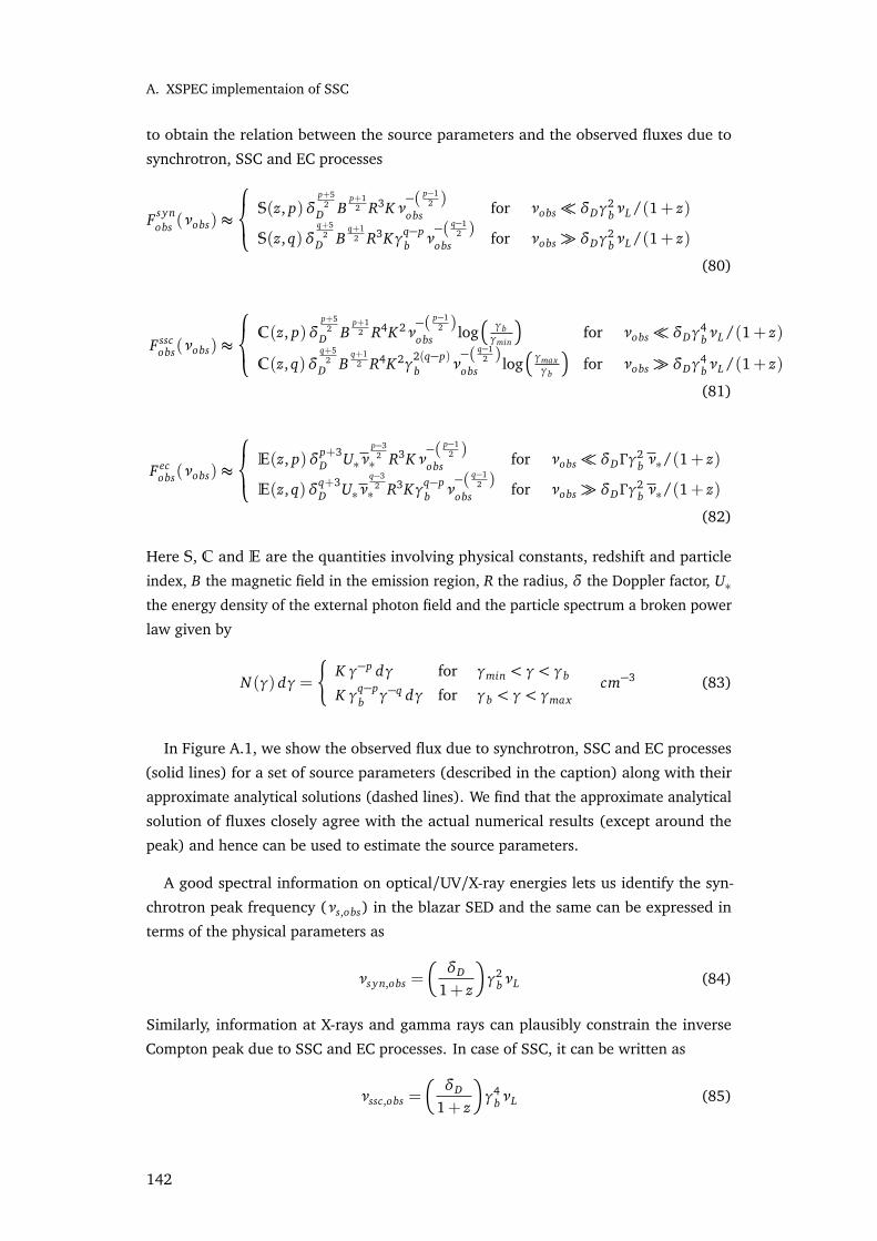
A. XSPEC implementaion of SSC
to obtain the relation between the source parameters and the observed fluxes due to
synchrotron, SSC and EC processes
F s ynobs (νobs) ≈
S(z, p)δp+5
2D B
p+12 R3Kν
−( p−12 )
obs for νobs δDγ2bνL/(1+ z)
S(z, q)δq+5
2D B
q+12 R3Kγq−p
b ν−( q−1
2 )obs for νobs δDγ
2bνL/(1+ z)
(80)
F sscobs(νobs) ≈
C(z, p)δp+5
2D B
p+12 R4K2ν
−( p−12 )
obs log
γbγmin
for νobs δDγ4bνL/(1+ z)
C(z, q)δq+5
2D B
q+12 R4K2γ
2(q−p)b ν
−( q−12 )
obs log
γmaxγb
for νobs δDγ4bνL/(1+ z)
(81)
F ecobs(νobs) ≈
E(z, p)δp+3D U∗ν
p−32∗ R3Kν
−( p−12 )
obs for νobs δDΓγ2b ν∗/(1+ z)
E(z, q)δq+3D U∗ν
q−32∗ R3Kγq−p
b ν−( q−1
2 )obs for νobs δDΓγ
2b ν∗/(1+ z)
(82)
Here S, C and E are the quantities involving physical constants, redshift and particle
index, B the magnetic field in the emission region, R the radius, δ the Doppler factor, U∗the energy density of the external photon field and the particle spectrum a broken power
law given by
N(γ) dγ=
¨
K γ−p dγ for γmin < γ < γb
K γq−pb γ−q dγ for γb < γ < γmax
cm−3 (83)
In Figure A.1, we show the observed flux due to synchrotron, SSC and EC processes
(solid lines) for a set of source parameters (described in the caption) along with their
approximate analytical solutions (dashed lines). We find that the approximate analytical
solution of fluxes closely agree with the actual numerical results (except around the
peak) and hence can be used to estimate the source parameters.
A good spectral information on optical/UV/X-ray energies lets us identify the syn-
chrotron peak frequency (νs,obs) in the blazar SED and the same can be expressed in
terms of the physical parameters as
νs yn,obs =
δD
1+ z
γ2bνL (84)
Similarly, information at X-rays and gamma rays can plausibly constrain the inverse
Compton peak due to SSC and EC processes. In case of SSC, it can be written as
νssc,obs =
δD
1+ z
γ4bνL (85)
142
A.1. Obtaining approximate guess values of physical parameters
1e-17
1e-16
1e-15
1e-14
1e-13
1e+10 1e+12 1e+14 1e+16 1e+18 1e+20 1e+22 1e+24 1e+26
ν F
ν (
erg
/cm
2/s
)
ν (Hz)
SynchrotronSSC
EC
Figure A.1.: The numerical synchrotron, SSC and EC spectrum (solid lines) with theirapproximate analytical equivalents (dashed lines). The model SED cor-responds to the following physical parameters: z = 0.536, p = 0.55,q = 1.5, K = 1× 10⁵, γmin = 10, γmax = 5× 10⁵, γb = 103, B = 0.1 G,Γ = 10.0, δD = 10.0, ν∗ = 5.86× 10¹³ Hz equivalent to temperature 1000 K,U∗ = 7.57×10⁻⁵ er g/cm3 and R = 1016 cm
and for the EC
νec,obs =
δDΓ
1+ z
γ2b ν∗ (86)
In addition to these, we can consider the particle energy density (Ue) and the magnetic
field energy density (UB) are related by
UB = ηUe (87)
where
UB =B2
8πer g/cm3 and Ue = mec2
γmax∫
γmin
γN(γ)dγ er g/cm3
Here, η ≈ 1 corresponds to the equipartition condition indicating total energy of the
system to be minimum. If the jet viewing angle can be anticipated, then it can constrain
the Doppler factor δD and the Lorentz factor Γ . In case of blazars, we can assume δD ≈ Γdue to small viewing angle. This, along with the knowledge of νs yn,obs, νssc,obs, νec,obs
and the fluxes at Optical (Synchrotron; equation (80)), X-ray (SSC; equation (81)) and
gamma-ray (EC; equation (82)), and the equipartition condition (87) can, in principle,
lets one estimate the source parameters by solving the relevant coupled equations. It
should be noted that we do not solve for γmin and γmax , which are weak parameters,
but rather choose them to be consistent with the observed SED. Besides these, we also
143

A. XSPEC implementaion of SSC
assume the external photon field to be a blackbody, illuminated by the accretion disk.
Then Uph∗ and ν∗ can be related by
ν∗ = 2.82 fex tKB
h
c4σSB
∫
Uph∗(νi∗) dνi∗
1/4
(88)
where KB is the Boltzmann constant, σSB is the Stefan-Boltzmann constant, Uph∗(νi∗) is
the blackbody energy density at frequency νi∗ and fex t is the covering factor.
A.2 X S P E C S P E C T R A L F I T
We developed numerical codes to calculate the emissivities corresponding to synchrotron,
SSC and EC emission processes which are then used to estimate the observed fluxes
after accounting for the relativistic and cosmological transformations. The codes were
optimized considerably by incorporating quadrature integrations and different interpola-
tion schemes to reduce the run time. These codes were then added as an additive local
models to the XSPEC package following the standard prescription1. The parameters of
the combined XSPEC models are the two particle indices p and q, minimum and the
maximum particle energies γmin and γmax , synchrotron peak frequency νps yn, SSC peak
frequency νpssc , EC peak frequency νp
ec , synchrotron flux F s yn at frequency νre fs yn, SSC flux
F ssc at frequency νre fssc , EC flux F ec at frequency νre f
ec and equipartition factor η 2. In
order to facilitate a faster convergence as well as to avoid the uncertainty regarding
the correct choice of initial guess parameters, we fit the observed fluxes corresponding
to synchrotron, SSC and EC processes, and peak frequencies. The physical parameters
required to obtain the exact emissivities were then calculated by solving the approxi-
mate coupled equations and other conditions described in the earlier section. The same
procedure was then used to extract back the best fit physical parameters from the fitted
observational quantities. Model systematics of 10% were assumed.
In Figure A.2 show the results of our fitting on the observed SED of 3C 279 during a
flare in April 2014.
1 http://heasarc.gsfc.nasa.gov/docs/xanadu/xspec/manual/manual.html2 Here onwards all frequencies and fluxes are measured in the observer’s frame.
144

A.2. XSPEC Spectral fit
1e-13
1e-12
1e-11
1e-10
1e-09
1e-08
1e+10 1e+12 1e+14 1e+16 1e+18 1e+20 1e+22 1e+24 1e+26
ν F
ν(e
rgs/c
m2/s
)
ν(Hz)
SMARTS/Swift UVOTSwift XRT
Fermi
(a) Observed SED
0.01
0.1
keV
2 (P
hoto
ns c
m−
2 s−
1 ke
V−
1 )
Unfolded Spectrum
10−3 0.01 0.1 1 10 100 1000 104 105 106
−2
−1
0
1
χ
Energy (keV)
(b) Best fit XSPEC model
Figure A.2.: The observed SED of 3C 279 during a flare in April 2014 (Paliya et al.,2015b) fitted with the developed zone SSC+EC module in XSPEC. Thebottom panel shows the residual χ2.
145

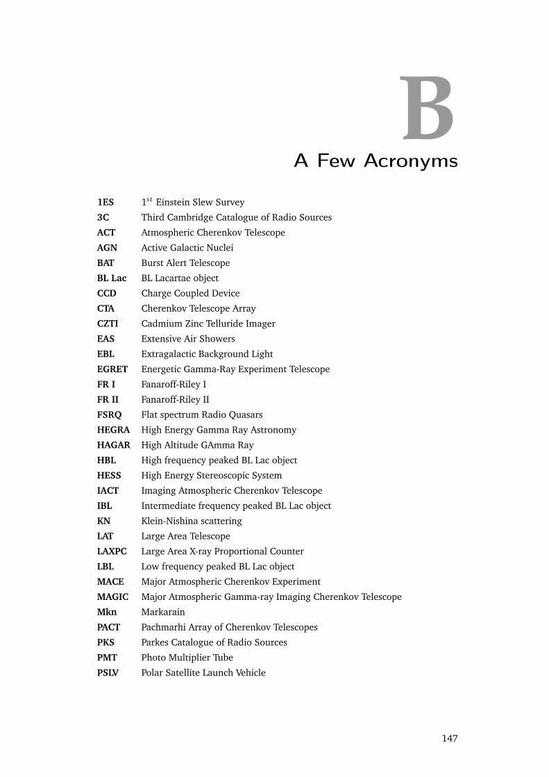
BA Few Acronyms
1ES 1st Einstein Slew Survey
3C Third Cambridge Catalogue of Radio Sources
ACT Atmospheric Cherenkov Telescope
AGN Active Galactic Nuclei
BAT Burst Alert Telescope
BL Lac BL Lacartae object
CCD Charge Coupled Device
CTA Cherenkov Telescope Array
CZTI Cadmium Zinc Telluride Imager
EAS Extensive Air Showers
EBL Extragalactic Background Light
EGRET Energetic Gamma-Ray Experiment Telescope
FR I Fanaroff-Riley I
FR II Fanaroff-Riley II
FSRQ Flat spectrum Radio Quasars
HEGRA High Energy Gamma Ray Astronomy
HAGAR High Altitude GAmma Ray
HBL High frequency peaked BL Lac object
HESS High Energy Stereoscopic System
IACT Imaging Atmospheric Cherenkov Telescope
IBL Intermediate frequency peaked BL Lac object
KN Klein-Nishina scattering
LAT Large Area Telescope
LAXPC Large Area X-ray Proportional Counter
LBL Low frequency peaked BL Lac object
MACE Major Atmospheric Cherenkov Experiment
MAGIC Major Atmospheric Gamma-ray Imaging Cherenkov Telescope
Mkn Markarain
PACT Pachmarhi Array of Cherenkov Telescopes
PKS Parkes Catalogue of Radio Sources
PMT Photo Multiplier Tube
PSLV Polar Satellite Launch Vehicle
147

B. A Few Acronyms
SED Spectral Energy Distribution
SSA Synchrotron Self Absorption
SSC Synchrotron Self Compton
SSM Scanning Sky Moniter
STACEE Solar Tower Atmospheric Cherenkov Effect Experiment
SXT Soft X-ray Telescope
UVIT UltraViolet Imaging Telescope
UVOT UltraViolet Optical Telescope
VERITAS Very Energetic Radiation Imaging Telescope Array System
VHE Very High Energy
XRT X-ray Telescope
XSPEC X-Ray Spectral Fitting Package
148

Bibliography
A. A. Abdo, et al. (2010a). ‘The Spectral Energy Distribution of Fermi Bright Blazars’.
ApJ 716, 30-70.
A. A. Abdo, et al. (2010b). ‘Fermi Large Area Telescope First Source Catalog’. ApJS 188,
405-436.
A. A. Abdo, et al. (2010c). ‘Fermi Large Area Telescope Constraints on the Gamma-ray
Opacity of the Universe’. ApJ 723, 1082-1096.
A. A. Abdo, et al. (2011a). ‘Fermi Large Area Telescope Observations of Markarian 421:
The Missing Piece of its Spectral Energy Distribution’. ApJ 736, 131.
A. A. Abdo, et al. (2011b). ‘Multi-wavelength Observations of the Flaring Gamma-ray
Blazar 3C 66A in 2008 October’. ApJ 726, 43.
V. Acciari, et al. (2009a). ‘Discovery of Very High Energy Gamma-ray Radiation from the
BL Lac 1ES 0806+524’. ApJL 690, L126-L129.
V. A. Acciari, et al. (2010). ‘The Discovery of γ-Ray Emission from the Blazar RGB
J0710+591’. ApJL 715, L49-L55.
V. A. Acciari, et al. (2009b). ‘VERITAS Observations of the BL Lac Object 1ES 1218+304’.
ApJ 695, 1370-1375.
V. A. Acciari, et al. (2009c). ‘Multiwavelength Observations of a TeV-Flare from W Comae’.
ApJ 707, 612-620.
V. A. Acciari, et al. (2009d). ‘Simultaneous Multiwavelength Observations of Markarian
421 During Outburst’. ApJ 703, 169-178.
F. Acero, et al. (2015). ‘Fermi Large Area Telescope Third Source Catalog’. ApJS 218, 23.
B. Acharya, et al. (2013). ‘Introducing the CTA concept’. Astroparticle Physics 43, 3 - 18.
B. S. Acharya, et al. (2013). ‘Monitoring of Blazars from HAGAR Cherenkov Telescope
Array’. In Proceedings of International Cosmic Ray Conference, 2013.
A. Achterberg & L. Ball (1994). ‘Particle acceleration at superluminal quasi-perpendicular
shocks. Application to SN1978K and SN1987A’. A&A 285, 687-704.
M. Ackermann, et al. (2011). ‘The Second Catalog of Active Galactic Nuclei Detected by
the Fermi Large Area Telescope’. ApJ 743, 171.
M. Ackermann, et al. (2012). ‘The Imprint of the Extragalactic Background Light in the
Gamma-Ray Spectra of Blazars’. Science 338, 1190.
149

Bibliography
F. Aharonian, et al. (2010). ‘Discovery of VHE γ-rays from the BL Lacertae object PKS
0548-322’. A&A 521, A69.
F. Aharonian, et al. (2009). ‘Simultaneous Observations of PKS 2155-304 with HESS,
Fermi, RXTE, and Atom: Spectral Energy Distributions and Variability in a Low State’.
ApJL 696, L150-L155.
F. Aharonian, et al. (2007a). ‘New constraints on the mid-IR EBL from the HESS discovery
of VHE γ-rays from 1ES 0229+200’. A&A 475, L9-L13.
F. Aharonian, et al. (2007b). ‘Discovery of VHE γ-rays from the distant BL Lacertae 1ES
0347-121’. A&A 473, L25-L28.
F. Aharonian, et al. (2008a). ‘Discovery of VHE γ-rays from the high-frequency-peaked
BL Lacertae object RGB J0152+017’. A&A 481, L103-L107.
F. Aharonian, et al. (2007c). ‘An Exceptional Very High Energy Gamma-Ray Flare of PKS
2155-304’. ApJL 664, L71-L74.
F. Aharonian, et al. (2006a). ‘Discovery of very high energy γ-ray emission from the BL
Lacertae object H 2356-309 with the HESS Cherenkov telescopes’. A&A 455, 461-466.
F. Aharonian, et al. (2006b). ‘A low level of extragalactic background light as revealed
by γ-rays from blazars’. Nature 440, 1018-1021.
F. A. Aharonian (2004). Very high energy cosmic gamma radiation : a crucial window on
the extreme Universe.
F. A. Aharonian (2013). ‘Gamma rays from supernova remnants’. Astroparticle Physics
43, 71 - 80.
F. A. Aharonian, et al. (2000). ‘The Energy Spectrum of TEV Gamma Rays from the Crab
Nebula as Measured by the HEGRA System of Imaging Air Cerenkov Telescopes’. ApJ
539, 317-324.
F. A. Aharonian, et al. (2008b). ‘Formation of hard very high energy gamma-ray spectra
of blazars due to internal photon-photon absorption’. MNRAS 387, 1206-1214.
M. L. Ahnen, et al. (2016a). ‘Search for VHE gamma-ray emission from Geminga pulsar
and nebula with the MAGIC telescopes’. ArXiv e-prints arXiv:1603.00730.
M. L. Ahnen, et al. (2016b). ‘MAGIC observations of the February 2014 flare of 1ES
1011+496 and ensuing constraint of the EBL density’. A&A 590, A24.
M. L. Ahnen, et al. (2016c). ‘Multiwavelength observations of the blazar 1ES 1011+496
in Spring 2008’. MNRAS 459, 2286-2298.
150
Bibliography
J. Albert, et al. (2006). ‘Discovery of Very High Energy γ-Rays from Markarian 180
Triggered by an Optical Outburst’. ApJL 648, L105-L108.
J. Albert, et al. (2007a). ‘Observations of Markarian 421 with the MAGIC Telescope’. ApJ
663, 125-138.
J. Albert, et al. (2007b). ‘Discovery of Very High Energy γ-Rays from 1ES 1011+496 at z
= 0.212’. ApJL 667, L21-L24.
J. Albert, et al. (2007c). ‘Observation of Very High Energy γ-Rays from the AGN 1ES
2344+514 in a Low Emission State with the MAGIC Telescope’. ApJ 662, 892-899.
J. Aleksic, et al. (2012a). ‘Discovery of VHE γ-rays from the blazar 1ES 1215+303 with
the MAGIC telescopes and simultaneous multi-wavelength observations’. A&A 544,
A142.
J. Aleksic, et al. (2012b). ‘Mrk 421 active state in 2008: the MAGIC view, simultaneous
multi-wavelength observations and SSC model constrained’. A&A 542, A100.
J. Aleksic, et al. (2012c). ‘Discovery of VHE γ-ray emission from the BL Lacertae object
B3 2247+381 with the MAGIC telescopes’. A&A 539, A118.
J. Aleksic, et al. (2010). ‘MAGIC TeV gamma-ray observations of Markarian 421 during
multiwavelength campaigns in 2006’. A&A 519, A32.
J. Aleksic, et al. (2016). ‘Insights into the emission of the blazar 1ES 1011+496 through
unprecedented broadband observations during 2011 and 2012’. A&A 591, A10.
J. Aleksic, et al. (2014a). ‘Unprecedented study of the broadband emission of Mrk 421
during flaring activity in March 2010’. ArXiv e-prints arXiv:1412.3576.
J. Aleksic, et al. (2014b). ‘Discovery of very high energy gamma-ray emission from the
blazar 1ES 1727+502 with the MAGIC Telescopes’. A&A 563, A90.
J. Aleksic, et al. (2014c). ‘Rapid and multiband variability of the TeV bright active nucleus
of the galaxy IC 310’. A&A 563, A91.
J. Aleksic, et al. (2011). ‘MAGIC Discovery of Very High Energy Emission from the FSRQ
PKS 1222+21’. ApJL 730, L8.
T. Alexander (1997). ‘Is AGN Variability Correlated with Other AGN Properties? ZDCF
Analysis of Small Samples of Sparse Light Curves’. In D. Maoz, A. Sternberg, & E. M.
Leibowitz (eds.), Astronomical Time Series, vol. 218 of Astrophysics and Space Science
Library, p. 163.
E. Aliu, et al. (2012a). ‘Discovery of High-energy and Very High Energy γ-Ray Emission
from the Blazar RBS 0413’. ApJ 750, 94.
151
Bibliography
E. Aliu, et al. (2012b). ‘Multiwavelength Observations of the AGN 1ES 0414+009 with
VERITAS, Fermi-LAT, Swift-XRT, and MDM’. ApJ 755, 118.
E. Aliu, et al. (2011). ‘Multiwavelength Observations of the Previously Unidentified
Blazar RX J0648.7+1516’. ApJ 742, 127.
H. Anderhub, et al. (2009a). ‘Discovery of very High Energy γ-Rays from the Blazar S5
0716+714’. ApJL 704, L129-L133.
H. Anderhub, et al. (2009b). ‘Simultaneous Multiwavelength Observation of Mkn 501 in
a Low State in 2006’. ApJ 705, 1624-1631.
S. Antón & I. W. A. Browne (2005). ‘The recognition of blazars and the blazar spectral
sequence’. MNRAS 356, 225-231.
R. R. J. Antonucci (1984). ‘Optical spectropolarimetry of radio galaxies’. ApJ 278,
499-520.
A. M. Atoyan & F. A. Aharonian (1999). ‘Modelling of the non-thermal flares in the
Galactic microquasar GRS 1915+105’. MNRAS 302, 253-276.
W. B. Atwood, et al. (2009). ‘The Large Area Telescope on the Fermi Gamma-Ray Space
Telescope Mission’. ApJ 697, 1071-1102.
M. Balokovic, et al. (2013). ‘First Results from NuSTAR Observations of Mkn 421’. In
European Physical Journal Web of Conferences, vol. 61 of European Physical Journal Web
of Conferences, p. 4013.
S. D. Barthelmy, et al. (2005). ‘The Burst Alert Telescope (BAT) on the SWIFT Midex
Mission’. Space Sci. Rev. 120, 143-164.
B. Bartoli, et al. (2015). ‘4.5 years multi-wavelength observations of Mrk 421 during the
ARGO-YBJ and Fermi common operation time’. ArXiv e-prints arXiv:1511.06851.
W. H. Baumgartner, et al. (2013). ‘The 70 Month Swift-BAT All-sky Hard X-Ray Survey’.
ApJS 207, 19.
V. Beckmann & C. Shrader (2012a). ‘The AGN phenomenon: open issues’. In Proceedings
of ”An INTEGRAL view of the high-energy sky (the first 10 years)” - 9th INTEGRAL
Workshop and celebration of the 10th anniversary of the launch (INTEGRAL 2012).
15-19 October 2012. Bibliotheque Nationale de France, Paris, France., p. 69.
V. Beckmann & C. R. Shrader (2012b). Active Galactic Nuclei.
M. C. Begelman, et al. (2008). ‘Implications of very rapid TeV variability in blazars’.
MNRAS 384, L19-L23.
A. Bell (2013). ‘Cosmic ray acceleration’. Astroparticle Physics 43, 56 - 70.
152
Bibliography
L. Bergstrom (2013). ‘Dark matter and imaging air Cherenkov arrays’. Astroparticle
Physics 43, 44 - 49.
M. S. Bessell, et al. (1998). ‘Model atmospheres broad-band colors, bolometric corrections
and temperature calibrations for O - M stars’. A&A 333, 231-250.
V. Bhalerao (2012). Neutron Stars and NuSTAR. Ph.D. thesis, Caltech.
R. D. Blandford & A. Levinson (1995). ‘Pair cascades in extragalactic jets. 1: Gamma
rays’. ApJ 441, 79-95.
R. D. Blandford & R. L. Znajek (1977). ‘Electromagnetic extraction of energy from Kerr
black holes’. MNRAS 179, 433-456.
M. G. Blasi, et al. (2013). ‘The TeV blazar Markarian 421 at the highest spatial resolution’.
A&A 559, A75.
M. Błazejowski, et al. (2005). ‘A Multiwavelength View of the TeV Blazar Markarian 421:
Correlated Variability, Flaring, and Spectral Evolution’. ApJ 630, 130-141.
M. Błazejowski, et al. (2000). ‘Comptonization of Infrared Radiation from Hot Dust by
Relativistic Jets in Quasars’. ApJ 545, 107-116.
G. R. Blumenthal & R. J. Gould (1970). ‘Bremsstrahlung, Synchrotron Radiation, and
Compton Scattering of High-Energy Electrons Traversing Dilute Gases’. Reviews of
Modern Physics 42, 237-271.
M. Boettcher (2010). ‘Models for the Spectral Energy Distributions and Variability of
Blazars’. ArXiv e-prints arXiv:1006.5048.
D. Bose, et al. (2007). ‘Observations of AGNs using PACT’. APSS 309, 111-117.
M. Böttcher (2007). ‘Astrophysical Jets of Blazars and Microquasars’. APSS 307, 69-75.
M. Böttcher & J. Chiang (2002). ‘X-Ray Spectral Variability Signatures of Flares in BL
Lacertae Objects’. ApJ 581, 127-142.
M. Böttcher & C. D. Dermer (2002). ‘An Evolutionary Scenario for Blazar Unification’.
ApJ 564, 86-91.
M. Böttcher, et al. (2008). ‘The Hard VHE γ-Ray Emission in High-Redshift TeV Blazars:
Comptonization of Cosmic Microwave Background Radiation in an Extended Jet?’.
ApJL 679, L9.
M. Böttcher, et al. (2010). ‘Optical Spectral Variability of the Very High Energy Gamma-ray
Blazar 1ES 1011+496’. ApJ 725, 2344-2348.
M. Böttcher, et al. (2009). ‘Implications of the very High Energy Gamma-Ray Detection
of the Quasar 3C279’. ApJ 703, 1168-1175.
153

Bibliography
M. Böttcher, et al. (2013). ‘Leptonic and Hadronic Modeling of Fermi-detected Blazars’.
ApJ 768, 54.
A. A. Breeveld, et al. (2010). ‘Further calibration of the Swift ultraviolet/optical telescope’.
MNRAS 406, 1687-1700.
A. A. Breeveld, et al. (2011). ‘An Updated Ultraviolet Calibration for the Swift/UVOT’. In
J. E. McEnery, J. L. Racusin, & N. Gehrels (eds.), American Institute of Physics Conference
Series, vol. 1358 of American Institute of Physics Conference Series, pp. 373–376.
W. Brinkmann, et al. (2003). ‘Temporal variability of Mrk 421 from XMM-Newton
observations’. A&A 402, 929-947.
G. Brusa, et al. (2003). ‘MMT adaptive secondary: performance evaluation and field
testing’. In P. L. Wizinowich & D. Bonaccini (eds.), Adaptive Optical System Technologies
II, vol. 4839 of Society of Photo-Optical Instrumentation Engineers (SPIE) Conference
Series, pp. 691–702.
G. R. Burbidge (1959). ‘Estimates of the Total Energy in Particles and Magnetic Field in
the Non-Thermal Radio Sources.’. ApJ 129, 849-852.
D. N. Burrows, et al. (2005). ‘The Swift X-Ray Telescope’. Space Sci. Rev. 120, 165-195.
M. Cerruti (2015a). ‘VERITAS detection of gamma-ray flaring activity from the BL
Lac object 1ES 1727+502 during bright moonlight observations’. ArXiv e-prints
arXiv:1508.05551.
M. Cerruti (2015b). ‘Very-high-energy blazars: updates from VERITAS observations and
multi-wavelength campaigns’. ArXiv e-prints arXiv:1501.03554.
P. Chadwick (2012). ‘Cherenkov Telescope Array is set to open new windows’. http://cerncourier.com/cws/article/cern/50220. [Online; accessed 31-August-
2016].
J. S. Chang & G. Cooper (1970). ‘A Practical Difference Scheme for Fokker-Planck
Equations’. Journal of Computational Physics 6, 1-16.
J. Chevalier, et al. (2015). ‘Long term variability of the blazar PKS 2155-304’. ArXiv
e-prints arXiv:1509.03104.
M. Chiaberge & G. Ghisellini (1999). ‘Rapid variability in the synchrotron self-Compton
model for blazars’. MNRAS 306, 551-560.
V. R. Chitnis, et al. (2011). ‘Status of HAGAR Telescope Array in Himalayas’. Proceedings
of 32nd International Cosmic Ray Conference held at Beijing, China 9, 166.
V. R. Chitnis, et al. (2009). ‘X-Ray Variability of Active Galactic Nuclei in the Soft and
Hard X-Ray Bands’. ApJ 698, 1207-1220.
154
Bibliography
V. R. Chitnis, et al. (2015). ‘Very high energy gamma ray astronomy using HAGAR
Telescope System’. In CURRENT ISSUES IN COSMOLOGY, ASTROPHYSICS AND HIGH
ENERGY PHYSICS, vol. 1, pp. 16–26.
J. Condon (2016). ‘Synchrotron Spectrum’. http://www.cv.nrao.edu/course/astr534/SynchrotronSpectrum.html. [Online; accessed 31-August-2016].
A. Cooray (2016). ‘Extragalactic background light measurements and applications’. Royal
Society open science 3, 150555.
P. S. Coppi & F. A. Aharonian (1999). ‘Simultaneous X-Ray and Gamma-Ray Observations
of TEV Blazars: Testing Synchro-Compton Emission Models and Probing the Infrared
Extragalactic Background’. ApJL 521, L33-L36.
R. H. D. Corbet & C. R. Shrader (2014). ‘Confirmation of High-Flux State of 1ES 1011+496
(= 2FGL J1015.1+4925) from Fermi LAT Automated Analysis’. The Astronomer’s
Telegram 5888, 1.
J. Cortina & J. Holder (2013). ‘MAGIC and VERITAS detect an unprecedented flaring
activity from Mrk 421 in very high energy gamma-rays’. The Astronomer’s Telegram
4976, 1.
L. Costamante & G. Ghisellini (2002). ‘TeV candidate BL Lac objects’. A&A 384, 56-71.
L. Costamante, et al. (2001). ‘Extreme synchrotron BL Lac objects. Stretching the blazar
sequence’. A&A 371, 512-526.
W. Cui (2004). ‘X-Ray Flaring Activity of Markarian 421’. ApJ 605, 662-669.
A. De Angelis, et al. (2013). ‘Transparency of the Universe to gamma-rays’. MNRAS 432,
3245-3249.
A. de Angelis, et al. (2009). ‘Photon propagation and the very high energy γ-ray spectra
of blazars: how transparent is the Universe?’. MNRAS 394, L21-L25.
C. D. Dermer & G. Menon (2009). High Energy Radiation from Black Holes: Gamma Rays,
Cosmic Rays, and Neutrinos.
C. D. Dermer & R. Schlickeiser (1993). ‘Model for the High-Energy Emission from Blazars’.
ApJ 416, 458.
C. D. Dermer, et al. (1992). ‘High-energy gamma radiation from extragalactic radio
sources’. A&A 256, L27-L30.
C. D. Dermer, et al. (1997). ‘Nonthermal Compton and Synchrotron Processes in the
Jets of Active Galactic Nuclei’. ApJS 109, 103-137.
155
Bibliography
A. Domínguez, et al. (2013). ‘Detection of the Cosmic γ-Ray Horizon from Multiwave-
length Observations of Blazars’. ApJ 770, 77.
A. Domínguez, et al. (2011). ‘Extragalactic background light inferred from AEGIS
galaxy-SED-type fractions’. MNRAS 410, 2556-2578.
D. Donato, et al. (2001). ‘Hard X-ray properties of blazars’. A&A 375, 739-751.
D. Donato, et al. (2005). ‘Six years of BeppoSAX observations of blazars: A spectral
catalog’. A&A 433, 1163-1169.
L. Dondi & G. Ghisellini (1995). ‘Gamma-ray-loud blazars and beaming’. MNRAS 273,
583-595.
E. Dwek & F. Krennrich (2013). ‘The extragalactic background light and the gamma-ray
opacity of the universe’. Astroparticle Physics 43, 112-133.
J. Ellis & N. E. Mavromatos (2013). ‘Probes of Lorentz violation’. Astroparticle Physics
43, 50 - 55.
W. Essey & A. Kusenko (2010). ‘A new interpretation of the gamma-ray observations of
distant active galactic nuclei’. Astroparticle Physics 33, 81-85.
B. L. Fanaroff & J. M. Riley (1974). ‘The morphology of extragalactic radio sources of
high and low luminosity’. MNRAS 167, 31P-36P.
D. J. Fegan (1997). ‘TOPICAL REVIEW: ?/hadron separation at TeV energies’. Journal of
Physics G Nuclear Physics 23, 1013-1060.
E. Fermi (1949). ‘On the Origin of the Cosmic Radiation’. Phys. Rev. 75, 1169–1174.
J. D. Finke & S. Razzaque (2009). ‘Constraints on the Extragalactic Background Light
from very High Energy Gamma-Ray Observations of Blazars’. ApJ 698, 1761-1766.
J. D. Finke, et al. (2010). ‘Modeling the Extragalactic Background Light from Stars and
Dust’. ApJ 712, 238-249.
L. Foschini, et al. (2011). ‘Search for the shortest variability at gamma rays in flat-
spectrum radio quasars’. A&A 530, A77.
G. Fossati, et al. (2008). ‘Multiwavelength Observations of Markarian 421 in 2001 March:
An Unprecedented View on the X-Ray/TeV Correlated Variability’. ApJ 677, 906-925.
G. Fossati, et al. (2000). ‘X-Ray Emission of Markarian 421: New Clues from Its Spectral
Evolution. II. Spectral Analysis and Physical Constraints’. ApJ 541, 166-179.
G. Fossati, et al. (1998). ‘A unifying view of the spectral energy distributions of blazars’.
MNRAS 299, 433-448.
156
Bibliography
A. Franceschini, et al. (2008). ‘Extragalactic optical-infrared background radiation, its
time evolution and the cosmic photon-photon opacity’. A&A 487, 837-852.
A. Furniss, et al. (2013). ‘The Firm Redshift Lower Limit of the Most Distant TeV-detected
Blazar PKS 1424+240’. ApJL 768, L31.
J. A. Gaidos, et al. (1996). ‘Extremely rapid bursts of TeV photons from the active galaxy
Markarian 421’. Nature 383, 319-320.
W. Galbraith & J. V. Jelley (1953). ‘Light Pulses from the Night Sky associated with
Cosmic Rays’. Nature 171, 349-350.
H. Gaur, et al. (2012). ‘Multiwavelength Variability of the Blazars Mrk 421 and 3C 454.3
in the High State’. AJ 143, 23.
M. Georganopoulos & D. Kazanas (2003). ‘Decelerating Flows in TeV Blazars: A Resolu-
tion to the BL Lacertae-FR I Unification Problem’. ApJL 594, L27-L30.
M. Georganopoulos, et al. (2001). ‘The Beaming Pattern and Spectrum of Radiation
from Inverse Compton Scattering in Blazars’. ApJ 561, 111-117.
G. Ghisellini (ed.) (2013). Radiative Processes in High Energy Astrophysics, vol. 873 of
Lecture Notes in Physics, Berlin Springer Verlag.
G. Ghisellini (2015). ‘Swift for blazars’. Journal of High Energy Astrophysics 7, 163-172.
G. Ghisellini (2016). ‘The Blazar Sequence 2.0’. Galaxies 4, 36.
G. Ghisellini & P. Madau (1996). ‘On the origin of the gamma-ray emission in blazars’.
MNRAS 280, 67-76.
G. Ghisellini, et al. (1996). ‘Diagnostics of Inverse-Compton models for the γ-ray emission
of 3C 279 and MKN 421.’. A&AS 120, C503.
G. Ghisellini, et al. (2009). ‘The Fermi blazars’ divide’. MNRAS 396, L105-L109.
G. Ghisellini, et al. (1993). ‘Relativistic bulk motion in active galactic nuclei’. ApJ 407,
65-82.
G. Ghisellini & F. Tavecchio (2008). ‘The blazar sequence: a new perspective’. MNRAS
387, 1669-1680.
G. Ghisellini & F. Tavecchio (2009). ‘Canonical high-power blazars’. MNRAS 397, 985-
1002.
G. Ghisellini, et al. (2014). ‘The power of relativistic jets is larger than the luminosity of
their accretion disks’. Nature 515, 376-378.
157
Bibliography
D. Giannios (2013). ‘Reconnection-driven plasmoids in blazars: fast flares on a slow
envelope’. MNRAS 431, 355-363.
B. Giebels & B. Degrange (2009). ‘Lognormal variability in BL Lacertae’. A&A 503,
797-799.
R. C. Gilmore, et al. (2009). ‘GeV gamma-ray attenuation and the high-redshift UV
background’. MNRAS 399, 1694-1708.
P. Giommi, et al. (2012). ‘A simplified view of blazars: clearing the fog around long-
standing selection effects’. MNRAS 420, 2899-2911.
K. S. Gothe, et al. (2013). ‘Pointing of HAGAR telescope mirrors’. Experimental Astronomy
35, 489-506.
R. J. Gould & G. P. Schréder (1967). ‘Opacity of the Universe to High-Energy Photons’.
Physical Review 155, 1408-1411.
X. Guangzhong, et al. (1988). ‘Optical behaviour of 8 BL Lac objects and the properties
of their central nucleus’. A&AS 72, 163-169.
A. C. Gupta, et al. (2004). ‘Near infrared intraday variability of Mrk 421’. A&A 422,
505-508.
J. Guy, et al. (2000). ‘Constraints on the cosmic infra-red background based on BeppoSAX
and CAT spectra of Markarian 501’. A&A 359, 419-428.
F. A. Harrison, et al. (2013). ‘The Nuclear Spectroscopic Telescope Array (NuSTAR)
High-energy X-Ray Mission’. ApJ 770, 103.
R. C. Hartman, et al. (1999). ‘The Third EGRET Catalog of High-Energy Gamma-Ray
Sources’. ApJS 123, 79-202.
M. G. Hauser, et al. (1998). ‘The COBE Diffuse Infrared Background Experiment Search
for the Cosmic Infrared Background. I. Limits and Detections’. ApJ 508, 25-43.
M. G. Hauser & E. Dwek (2001). ‘The Cosmic Infrared Background: Measurements and
Implications’. ARA&A 39, 249-307.
P. Hazarika, et al. (2015). ‘Observations of blazars 1ES 1426+428, 1ES 1218+304 and
3C 454.3 by HAGAR Telescope’. In CURRENT ISSUES IN COSMOLOGY, ASTROPHYSICS
AND HIGH ENERGY PHYSICS, vol. 1, pp. 154–159.
D. Heck, et al. (1998). CORSIKA: a Monte Carlo code to simulate extensive air showers.
W. Heitler (1937). ‘On the Analysis of Cosmic Rays’. Proceedings of the Royal Society of
London Series A 161, 261-283.
158
Bibliography
K. Helgason & A. Kashlinsky (2012). ‘Reconstructing the γ-Ray Photon Optical Depth of
the Universe to z ˜ 4 from Multiwavelength Galaxy Survey Data’. ApJL 758, L13.
H.E.S.S. Collaboration, et al. (2013a). ‘Discovery of very high energy γ-ray emission
from the BL Lacertae object PKS 0301-243 with H.E.S.S.’. A&A 559, A136.
H.E.S.S. Collaboration, et al. (2013b). ‘Discovery of high and very high-energy emission
from the BL Lacertae object SHBL J001355.9-185406’. A&A 554, A72.
HESS Collaboration, et al. (2013). ‘HESS and Fermi-LAT discovery of γ-rays from the
blazar 1ES 1312−423’. MNRAS 434, 1889-1901.
H.E.S.S. Collaboration, et al. (2013). ‘Measurement of the extragalactic background light
imprint on the spectra of the brightest blazars observed with H.E.S.S.’. A&A 550, A4.
H.E.S.S. Collaboration, et al. (2012). ‘Discovery of VHE γ-ray emission and multi-
wavelength observations of the BL Lacertae object 1RXS J101015.9-311909’. A&A
542, A94.
H.E.S.S. Collaboration, et al. (2011). ‘Simultaneous multi-wavelength campaign on PKS
2005-489 in a high state’. A&A 533, A110.
A. M. Hillas (2013). ‘Evolution of ground-based gamma-ray astronomy from the early
days to the Cherenkov Telescope Arrays’. Astroparticle Physics 43, 19-43.
D. Horan, et al. (2009). ‘Multiwavelength Observations of Markarian 421 in 2005-2006’.
ApJ 695, 596-618.
F. Hoyle & W. A. Fowler (1963a). ‘Nature of Strong Radio Sources’. Nature 197, 533-535.
F. Hoyle & W. A. Fowler (1963b). ‘On the nature of strong radio sources’. MNRAS 125,
169.
N. Isobe, et al. (2010). ‘Bright X-Ray Flares from the BL Lac Object Markarian 421,
Detected with MAXI in 2010 January and February’. PASJ 62, L55.
S. jie Qian, et al. (1998). ‘Correlation between TeV and X-ray bursts in Mrk 421’. Chinese
Astronomy and Astrophysics 22, 155 - 160.
M. Joshi (2009). Spectral variability studies and acceleration scenarios in jets of blazars.
Ph.D. thesis, Ohio University.
K. Katarzynski, et al. (2005). ‘Correlation between the TeV and X-ray emission in high-
energy peaked BLÂaLac objects’. A&A 433, 479-496.
P. M. W. Kalberla, et al. (2005). ‘The Leiden/Argentine/Bonn (LAB) Survey of Galactic HI.
Final data release of the combined LDS and IAR surveys with improved stray-radiation
corrections’. A&A 440, 775-782.
159
Bibliography
B. Kapanadze (2014). ‘The Highest Historical 0.3-10 keV Flux in TeV Blazar 1ES
1011+496’. The Astronomer’s Telegram 5866, 1.
N. S. Kardashev (1962). ‘Nonstationarity of Spectra of Young Sources of Nonthermal
Radio Emission’. Soviet Ast. 6, 317.
J. Kataoka, et al. (2000). ‘Variability Pattern and the Spectral Evolution of the BL Lacertae
Object PKS 2155-304’. ApJ 528, 243-253.
K. Katarzynski, et al. (2006). ‘Hard TeV spectra of blazars and the constraints to the
infrared intergalactic background’. MNRAS 368, L52-L56.
S. R. Kelner, et al. (2006). ‘Energy spectra of gamma rays, electrons, and neutrinos
produced at proton-proton interactions in the very high energy regime’. Phys. Rev. D
74, 034018.
T. Kelsall, et al. (1998). ‘The COBE Diffuse Infrared Background Experiment Search for
the Cosmic Infrared Background. II. Model of the Interplanetary Dust Cloud’. ApJ 508,
44-73.
A. D. Kerrick, et al. (1995). ‘Outburst of TeV photons from Markarian 421’. ApJL 438,
L59-L62.
J. G. Kirk, et al. (1994). ‘Radio emission from SNR 1987A’. ApJS 90, 807-811.
J. G. Kirk, et al. (1998). ‘Particle acceleration and synchrotron emission in blazar jets’.
A&A 333, 452-458.
T. M. Kneiske & H. Dole (2010). ‘A lower-limit flux for the extragalactic background
light’. A&A 515, A19.
R. Koul, et al. (2011). ‘An update on the design and implementation of the MACE
gamma-ray telescope’. Proceedings of the 32nd International Cosmic Ray Conference
held at Beiging, China 9, 107.
H. Krawczynski, et al. (2004). ‘Multiwavelength Observations of Strong Flares from the
TeV Blazar 1ES 1959+650’. ApJ 601, 151-164.
H. Krawczynski, et al. (2001). ‘Simultaneous X-Ray and TeV Gamma-Ray Observation of
the TeV Blazar Markarian 421 during 2000 February and May’. ApJ 559, 187-195.
F. Krennrich, et al. (2008). ‘Constraints on Energy Spectra of Blazars based on Recent
EBL Limits from Galaxy Counts’. ApJL 689, L93.
J. H. Krolik (1999). Active galactic nuclei : from the central black hole to the galactic
environment.
160
Bibliography
P. Kushwaha, et al. (2016). ‘Evidence for Two Lognormal States in Multi-wavelength
Flux Variation of FSRQ PKS 1510-089’. ApJL 822, L13.
P. Kushwaha, et al. (2014). ‘Gamma-ray flare of PKS 1222+216 in 2010: effect of jet
dynamics at the recollimation zone’. MNRAS 442, 131-137.
E. Lefa, et al. (2011). ‘Formation of Very Hard Gamma-Ray Spectra of Blazars in Leptonic
Models’. ApJ 740, 64.
B. Li, et al. (2013). ‘Correlation between X-ray and γ-ray for Fermi blazars’. APSS 347,
349-355.
H. Li & M. Kusunose (2000). ‘Temporal and Spectral Variabilities of High-Energy Emission
from Blazars Using Synchrotron Self-Compton Models’. ApJ 536, 729-741.
G. G. Lichti, et al. (2008). ‘INTEGRAL observations of the blazar Mrk 421 in outburst.
Results of a multi-wavelength campaign’. A&A 486, 721-734.
Y. C. Lin, et al. (1992). ‘Detection of high-energy gamma-ray emission from the BL
Lacertae object Markarian 421 by the EGRET telescope on the Compton Observatory’.
ApJL 401, L61-L64.
F. K. Liu, et al. (1997). ‘The long-term optical behavior of MKN 421’. A&AS 123, 569-574.
M. S. Longair (2011). High Energy Astrophysics.
D. Lynden-Bell (1969). ‘Galactic Nuclei as Collapsed Old Quasars’. Nature 223, 690-694.
P. Madau & E. S. Phinney (1996). ‘Constraints on the Extragalactic Background Light
from Gamma-Ray Observations of High-Redshift Quasars’. ApJ 456, 124.
P. Madau & L. Pozzetti (2000). ‘Deep galaxy counts, extragalactic background light and
the stellar baryon budget’. MNRAS 312, L9-L15.
MAGIC Collaboration, et al. (2008). ‘Very-High-Energy gamma rays from a Distant
Quasar: How Transparent Is the Universe?’. Science 320, 1752-.
M. A. Malkov & L. O. Drury (2001). ‘Nonlinear theory of diffusive acceleration of particles
by shock waves’. Reports on Progress in Physics 64, 429.
N. Mankuzhiyil (2010). MAGIC γ-RAY OBSERVATIONS OF DISTANT AGN AND A STUDY
OF SOURCE VARIABILITY AND THE EXTRAGALACTIC BACKGROUND LIGHT USING
FERMI AND AIR CHERENKOV TELESCOPES. Ph.D. thesis, MAGIC.
N. Mankuzhiyil, et al. (2012). ‘Emitting Electrons and Source Activity in Markarian 501’.
ApJ 753, 154.
161
Bibliography
N. Mankuzhiyil, et al. (2010). ‘High-frequency-peaked BL Lacertae Objects as Spectral
Candles to Measure the Extragalactic Background Light in the Fermi and Air Cherenkov
Telescopes Era’. ApJL 715, L16-L20.
K. Mannheim & P. L. Biermann (1989). ‘Photomeson production in active galactic nuclei’.
A&A 221, 211-220.
K. Mannheim & P. L. Biermann (1992). ‘Gamma-ray flaring of 3C 279 - A proton-initiated
cascade in the jet?’. A&A 253, L21-L24.
L. Maraschi, et al. (1992). ‘A jet model for the gamma-ray emitting blazar 3C 279’. ApJL
397, L5-L9.
A. P. Marscher & W. K. Gear (1985). ‘Models for high-frequency radio outbursts in
extragalactic sources, with application to the early 1983 millimeter-to-infrared flare of
3C 273’. ApJ 298, 114-127.
E. Massaro, et al. (2004). ‘Log-parabolic spectra and particle acceleration in the BL Lac
object Mkn 421: Spectral analysis of the complete BeppoSAX wide band X-ray data
set’. A&A 413, 489-503.
F. Massaro, et al. (2008). ‘X-ray spectral evolution of TeV BL Lacertae objects: eleven
years of observations with BeppoSAX, XMM-Newton and Swift satellites’. A&A 478,
395-401.
M. Matsuoka, et al. (2009). ‘The MAXI Mission on the ISS: Science and Instruments for
Monitoring All-Sky X-Ray Images’. PASJ 61, 999-.
D. Mazin & M. Raue (2007). ‘New limits on the density of the extragalactic background
light in the optical to the far infrared from the spectra of all known TeV blazars’. A&A
471, 439-452.
I. McHardy (2008). ‘Explaining X-ray Variability in Blazars’. In Blazar Variability across
the Electromagnetic Spectrum, p. 14.
C. Meegan, et al. (2009). ‘The Fermi Gamma-ray Burst Monitor’. ApJ 702, 791-804.
P. Meszaros (2013). ‘Gamma ray bursts’. Astroparticle Physics 43, 134 - 141.
M. Meyer, et al. (2012). ‘Limits on the extragalactic background light in the Fermi era’.
A&A 542, A59.
P. Mimica, et al. (2004). ‘Synthetic X-ray light curves of BL Lacs from relativistic hydro-
dynamic simulations’. A&A 418, 947-958.
R. Mirzoyan (2014). ‘Discovery of Very High Energy Gamma-Ray Emission From Gravita-
tionally Lensed Blazar S3 0218+357 With the MAGIC Telescopes’. The Astronomer’s
Telegram 6349.
162
Bibliography
R. Mirzoyan & J. Holder (2014). ‘Exceptionally high > 100 GeV flux state of 1ES
1011+496’. The Astronomer’s Telegram 5887, 1.
A. Moretti, et al. (2005). ‘In-flight calibration of the Swift XRT Point Spread Function’.
In O. H. W. Siegmund (ed.), UV, X-Ray, and Gamma-Ray Space Instrumentation for
Astronomy XIV, vol. 5898 of Society of Photo-Optical Instrumentation Engineers (SPIE)
Conference Series, pp. 360–368.
A. Mücke, et al. (2000). ‘Monte Carlo simulations of photohadronic processes in astro-
physics’. Computer Physics Communications 124, 290-314.
A. Mücke & R. J. Protheroe (2001). ‘A proton synchrotron blazar model for flaring in
Markarian 501’. Astroparticle Physics 15, 121-136.
T. Mufakharov, et al. (2015). ‘The observed radio/gamma-ray emission correlation for
blazars with the Fermi-LAT and the RATAN-600 data’. MNRAS 450, 2658-2669.
Y. I. Neshpor, et al. (2001). ‘Ultrahigh-Energy Gamma-Ray Emission from the Geminga
Pulsar’. Astronomy Letters 27, 228-232.
H. Netzer (2015). ‘Revisiting the Unified Model of Active Galactic Nuclei’. ARA&A 53,
365-408.
E. Nieppola, et al. (2006). ‘Spectral energy distributions of a large sample of BL Lacertae
objects’. A&A 445, 441-450.
K. Nilsson, et al. (2007). ‘Host galaxy subtraction of TeV candidate BL Lacertae objects’.
A&A 475, 199-207.
K. Nilsson, et al. (1999). ‘Two-dimensional Photometric Decomposition of the TeV BL
Lacertae Objects Markarian 421, Markarian 501, and 1ES 2344+514’. PASP 111,
1223-1232.
P. L. Nolan, et al. (2012). ‘Fermi Large Area Telescope Second Source Catalog’. ApJS 199,
31.
M. R. Orr, et al. (2011). ‘Strong New Constraints on the Extragalactic Background Light
in the Near- to Mid-infrared’. ApJ 733, 77.
A. G. Pacholczyk (1973). Radio astrophysics. Non-thermal processes in galactic and extra-
galactic sources.
P. Padovani & P. Giommi (1995). ‘The connection between x-ray- and radio-selected BL
Lacertae objects’. ApJ 444, 567-581.
V. S. Paliya, et al. (2015a). ‘Violent Hard X-ray Variability of Mrk 421 Observed by NuSTAR
in 2013 April’. ArXiv e-prints arXiv:1508.06399.
163
Bibliography
V. S. Paliya, et al. (2015b). ‘Multi-Wavelength Observations of 3C 279 During the
Extremely Bright Gamma-Ray Flare in 2014 March-April’. ApJ 803, 15.
B. Paul (2013). ‘Astrosat: Some Key Science Prospects’. International Journal of Modern
Physics D 22, 1341009.
E. S. Perlman, et al. (2006). ‘Intrinsic Curvature in the X-ray Spectra of BL Lacertae
Objects’. In H. R. Miller, K. Marshall, J. R. Webb, & M. F. Aller (eds.), Blazar Variability
Workshop II: Entering the GLAST Era, vol. 350 of Astronomical Society of the Pacific
Conference Series, p. 191.
E. S. Perlman, et al. (2005). ‘Intrinsic Curvature in the X-Ray Spectra of BL Lacertae
Objects’. ApJ 625, 727-740.
M. Petropoulou, et al. (2016). ‘Time-dependent neutrino emission from Mrk 421 during
flares and predictions for IceCube’. Astroparticle Physics 80, 115-130.
D. Petry, et al. (2002). ‘The TeV Spectrum of H1426+428’. ApJ 580, 104-109.
E. Pian, et al. (2014). ‘An active state of the BL Lacertae object Markarian 421 detected
by INTEGRAL in April 2013’. A&A 570, A77.
T. S. Poole, et al. (2008). ‘Photometric calibration of the Swift ultraviolet/optical tele-
scope’. MNRAS 383, 627-645.
E. Prandini, et al. (2010). ‘Constraining blazar distances with combined Fermi and TeV
data: an empirical approach’. MNRAS 405, L76-L80.
J. R. Primack, et al. (2005). ‘Observational Gamma-ray Cosmology’. In F. A. Aharonian,
H. J. Völk, & D. Horns (eds.), High Energy Gamma-Ray Astronomy, vol. 745 of American
Institute of Physics Conference Series, pp. 23–33.
M. Punch, et al. (1992). ‘Detection of TeV photons from the active galaxy Markarian
421’. Nature 358, 477.
A. B. Pushkarev, et al. (2010). ‘Radio/Gamma-ray Time Delay in the Parsec-scale Cores
of Active Galactic Nuclei’. ApJL 722, L7-L11.
J. P. Rachen & P. Mészáros (1998). ‘Photohadronic neutrinos from transients in astro-
physical sources’. Phys. Rev. D 58, 123005.
V. Ramakrishnan, et al. (2015). ‘Locating the γ-ray emission site in Fermi/LAT blazars
from correlation analysis between 37 GHz radio and γ-ray light curves’. MNRAS 452,
1280-1294.
A. R. Rao, et al. (2016). ‘AstroSat - a multi-wavelength astronomy satellite’. ArXiv e-prints
arXiv:1608.06051.
164

Bibliography
M. Raue & D. Mazin (2008). ‘Optical Depth for VHE γ-RAYS from Distant Sources from
a Generic EBL Density’. International Journal of Modern Physics D 17, 1515-1520.
R. Reesman & T. P. Walker (2013). ‘The TeV blazar measurement of the extragalactic
background light’. JCAP 12, 22.
A. Reimer & M. Bottcher (2013). ‘Studies of active galactic nuclei with CTA’. Astroparticle
Physics 43, 103 - 111.
A. Reimer, et al. (2008). ‘A Hard X-Ray View of Two Distant VHE Blazars: 1ES 1101-232
and 1ES 1553+113’. ApJ 682, 775-783.
J. L. Richards, et al. (2011). ‘Blazars in the Fermi Era: The OVRO 40 m Telescope
Monitoring Program’. ApJS 194, 29.
M. J. Ricketts, et al. (1976). ‘X-ray transient source at high galactic latitude and suggested
extragalactic identification’. Nature 259, 546.
P. Romano, et al. (2006). ‘Panchromatic study of GRB 060124: from precursor to
afterglow’. A&A 456, 917-927.
P. W. A. Roming, et al. (2005). ‘The Swift Ultra-Violet/Optical Telescope’. Space Sci. Rev.
120, 95-142.
G. B. Rybicki & A. P. Lightman (1986). Radiative Processes in Astrophysics.
L. Saha & P. Bhattacharjee (2015). ‘Constraints on the synchrotron self-Compton mech-
anism of TeV gamma ray emission from the Milagro TeV source MGRO J2019+37
within the pulsar wind nebula scenario’. Journal of High Energy Astrophysics 5-6, 9 -
14.
L. Saha, et al. (2013). ‘A study of the performance parameters of the High Altitude
Gamma Ray (HAGAR) telescope system at Ladakh in India’. Astroparticle Physics 42,
33-40.
S. Sahayanathan (2008). ‘A two-zone synchrotron model for the knots in the M87 jet’.
MNRAS 388, L49-L53.
S. Sahayanathan (2009). ‘Boundary shear acceleration in the jet of MKN501’. MNRAS
398, L49-L53.
S. Sahayanathan & S. Godambe (2012). ‘Modelling the very high energy flare of 3C 279
using one-zone leptonic model’. MNRAS 419, 1660-1666.
S. Sahayanathan & R. Misra (2005). ‘Interpretation of the Radio/X-Ray Knots of AGN
Jets within the Internal Shock Model Framework’. ApJ 628, 611-616.
165
Bibliography
S. Sahayanathan, et al. (2016). ‘Broadband Spectral Fitting of Blazars using XSPEC’. In
Prep. .
E. E. Salpeter (1964). ‘Accretion of Interstellar Matter by Massive Objects.’. ApJ 140,
796-800.
D. A. Sanchez, et al. (2013). ‘Evidence for a cosmological effect in γ-ray spectra of BL
Lacertae’. A&A 554, A75.
D. J. Schlegel, et al. (1998). ‘Maps of Dust Infrared Emission for Use in Estimation
of Reddening and Cosmic Microwave Background Radiation Foregrounds’. ApJ 500,
525-553.
M. Schmidt (1990). The discovery of quasars, p. 347.
M. Schroedter (2005). ‘Upper Limits on the Extragalactic Background Light from the
Very High Energy Gamma-Ray Spectra of Blazars’. ApJ 628, 617-628.
N. I. Shakura & R. A. Sunyaev (1973). ‘Black holes in binary systems. Observational
appearance.’. A&A 24, 337-355.
A. Shukla, et al. (2015). ‘Multi-frequency, Multi-epoch Study of Mrk 501: Hints for a
Two-component Nature of the Emission’. ApJ 798, 2.
A. Shukla, et al. (2012). ‘Multiwavelength study of the TeV blazar Mrk 421 during a
giant flare’. A&A 541, A140.
M. Sikora, et al. (1994). ‘Comptonization of diffuse ambient radiation by a relativistic
jet: The source of gamma rays from blazars?’. ApJ 421, 153-162.
M. Sikora, et al. (2001). ‘Modeling the Production of Flares in Gamma-Ray Quasars’.
ApJ 554, 1-11.
K. K. Singh, et al. (2014a). ‘Intrinsic VHE gamma-ray spectra of blazars as a probe for
extragalactic background light’. New Astronomy 27, 34-40.
K. K. Singh, et al. (2015). ‘Multi-wavelength study of Mrk 421 TeV flare observed with
TACTIC telescope in February 2010’. Astroparticle Physics 61, 32-40.
K. P. Singh, et al. (2014b). ‘ASTROSAT mission’. In Society of Photo-Optical Instrumentation
Engineers (SPIE) Conference Series, vol. 9144 of Society of Photo-Optical Instrumentation
Engineers (SPIE) Conference Series, p. 1.
A. Sinha, et al. (2016a). ‘On the spectral curvature of VHE blazar 1ES 1011+496: Effect
of spatial particle diffusion’. ApJ accepted .
A. Sinha, et al. (2014). ‘Estimation of the Extragalactic Background Light Using TeV
Observations of BL Lac Objects’. ApJ 795, 91.
166
Bibliography
A. Sinha, et al. (2015). ‘Underlying particle spectrum of Mkn 421 during the huge X-ray
flare in April 2013’. A&A 580, A100.
A. Sinha, et al. (2016b). ‘Long-term study of Mkn 421 with the HAGAR Array of
Telescopes’. A&A 591, A83.
P. S. Smith, et al. (2009). ‘Coordinated Fermi/Optical Monitoring of Blazars and the
Great 2009 September Gamma-ray Flare of 3C 454.3’. ArXiv e-prints arXiv:0912.3621.
A. Sokolov & A. P. Marscher (2005). ‘External Compton Radiation from Rapid Nonthermal
Flares in Blazars’. ApJ 629, 52-60.
D. Sowards-Emmerd, et al. (2003). ‘The Gamma-Ray Blazar Content of the Northern
Sky’. ApJ 590, 109-122.
T. Stanev & A. Franceschini (1998). ‘Constraints on the Extragalactic Infrared Background
from Gamma-Ray Observations of MRK 501’. ApJL 494, L159.
F. W. Stecker, et al. (2007). ‘Blazar γ-Rays, Shock Acceleration, and the Extragalactic
Background Light’. ApJL 667, L29-L32.
F. W. Stecker, et al. (2006). ‘Intergalactic Photon Spectra from the Far-IR to the UV Lyman
Limit for 0 < z > 6 and the Optical Depth of the Universe to High-Energy Gamma
Rays’. ApJ 648, 774-783.
F. W. Stecker & S. T. Scully (2006). ‘A Simple Analytic Treatment of the Intergalactic
Absorption Effect in Blazar Gamma-Ray Spectra’. ApJL 652, L9-L11.
F. W. Stecker & S. T. Scully (2010). ‘Derivation of a Relation for the Steepening of
Tev-Selected Blazar γ-ray Spectra with Energy and Redshift’. ApJL 709, L124-L126.
B. Sunder Sahayanathan (2011). ‘Broadband spectral modelling of bent jets of Active
Galactic Nuclei’. ArXiv e-prints arXiv:1109.0618.
C. Tadhunter (2008). ‘An introduction to active galactic nuclei: Classification and
unification’. Proceedings of the VLTI Euro Summer School Held in Torun, Poland 52,
227-239.
G. Tagliaferri, et al. (2008). ‘Simultaneous Multiwavelength Observations of the Blazar
1ES 1959+650 at a Low TeV Flux’. ApJ 679, 1029-1039.
T. Takahashi, et al. (1995). ‘Markarian 421’. IAU Circ 6167.
T. Takahashi, et al. (1994). ‘Markarian 421’. IAU Circ 5993.
T. Takahashi, et al. (1996). ‘ASCA Observation of an X-Ray/TeV Flare from the BL Lacertae
Object Markarian 421’. ApJL 470, L89.
167
Bibliography
Y. T. Tanaka, et al. (2014). ‘Extreme Blazars Studied with Fermi-LAT and Suzaku: 1ES
0347-121 and Blazar Candidate HESS J1943+213’. ArXiv e-prints arXiv:1404.3727.
F. Tavecchio (2014). ‘On the hadronic cascade scenario for extreme BL Lacs’. MNRAS
438, 3255-3262.
F. Tavecchio, et al. (2011). ‘On the origin of the γ-ray emission from the flaring blazar
PKS 1222+216’. A&A 534, A86.
F. Tavecchio & G. Ghisellini (2008). ‘Spine-sheath layer radiative interplay in subparsec-
scale jets and the TeV emission from M87’. MNRAS 385, L98-L102.
F. Tavecchio, et al. (1998). ‘Constraints on the Physical Parameters of TeV Blazars’. ApJ
509, 608-619.
M. Tluczykont, et al. (2010). ‘Long-term lightcurves from combined unified very high
energy γ-ray data’. A&A 524, A48.
J. A. Tomsick, et al. (2014). ‘The Reflection Component from Cygnus X-1 in the Soft
State Measured by NuSTAR and Suzaku’. The Astrophysical Journal 780, 78.
A. Tramacere, et al. (2007). ‘SWIFT observations of TeV BL Lacertae objects’. A&A 467,
501-508.
A. Tramacere, et al. (2009). ‘Swift observations of the very intense flaring activity of Mrk
421 during 2006. I. Phenomenological picture of electron acceleration and predictions
for MeV/GeV emission’. A&A 501, 879-898.
M.-H. Ulrich, et al. (1975). ‘Nonthermal continuum radiation in three elliptical galaxies’.
ApJ 198, 261-266.
C. M. Urry & P. Padovani (1995). ‘Unified Schemes for Radio-Loud Active Galactic Nuclei’.
PASP 107, 803.
M. Ushio, et al. (2010). ‘A Novel Approach in Constraining Electron Spectra in Blazar
Jets: The Case of Markarian 421’. ApJ 724, 1509-1516.
M. Ushio, et al. (2009). ‘Suzaku Wide Band Analysis of the X-Ray Variability of TeV Blazar
Mrk 421 in 2006’. ApJ 699, 1964-1972.
P. Uttley & I. M. McHardy (2001). ‘The flux-dependent amplitude of broadband noise
variability in X-ray binaries and active galaxies’. MNRAS 323, L26-L30.
R. Vainio, et al. (2004). ‘Conversion of bulk kinetic energy into radiation in AGNs and
GRBs: Particle transport effects’. A&A 414, 463-474.
V. V. Vassiliev (2000). ‘Extragalactic background light absorption signal in the TeV γ-ray
spectra of blazars’. Astroparticle Physics 12, 217-238.
168

Bibliography
S. Vaughan, et al. (2003). ‘On characterizing the variability properties of X-ray light
curves from active galaxies’. MNRAS 345, 1271-1284.
W. Brinkmann, et al. (2001). ‘XMM-Newton observations of Markarian 421’. A&A 365,
L162-L167.
S. Wakely & D. Horan (2016). ‘TeVcat’. http://tevcat.uchicago.edu/. [Online;
accessed 31-August-2016].
T. C. Weekes, et al. (1989). ‘Observation of TeV gamma rays from the Crab nebula using
the atmospheric Cerenkov imaging technique’. ApJ 342, 379-395.
M. Weidinger, et al. (2010). ‘Modelling the steady state spectral energy distribution of
the BL-Lac Object PKS 2155-30.4 using a selfconsistent SSC model’. Astrophysics and
Space Sciences Transactions 6, 1-7.
M. Weidinger & F. Spanier (2015). ‘A self-consistent and time-dependent hybrid blazar
emission model. Properties and application’. A&A 573, A7.
E. L. Wright (1998). ‘Angular Power Spectra of the COBE DIRBE Maps’. ApJ 496, 1.
D.-X. Wu, et al. (2014). ‘Correlation between γ-ray and radio emissions
in Fermi blazars’. Publications of the Astronomical Society of Japan 66,
http://pasj.oxfordjournals.org/content/66/6/117.full.pdf+html.
J. Yang & J. Wang (2010). ‘Constraining extragalactic background light from TeV blazars’.
A&A 522, A12.
O. Zacharopoulou, et al. (2011). ‘Modeling the Hard TeV Spectra of Blazars 1ES
0229+200 and 3C 66A with an Internal Absorption Scenario’. ApJ 738, 157.
F. J. Zhang & L. B. Bååth (1996). ‘Viewing Angles in Some Selected BL Lac Objects’. APSS
235, 195-205.
F. J. Zhang & L. B. Baath (1991). ‘The submilliarcsecond radio structures of the two BL
Lac objects Mkn421 and 0735 + 178’. MNRAS 248, 566-571.
Y. H. Zhang, et al. (2005). ‘XMM-Newton View of PKS 2155-304: Characterizing the
X-Ray Variability Properties with EPIC pn’. ApJ 629, 686-699.
169