a neural architecture based on the adaptive … neural architecture based on the adaptive resonant...

Flávio Henrique Teles Vieira, Luan Ling Lee 45

International Journal of Computer Science & Applications 2007 Technomathematics Research Foundation Vol. 4 Issue 3, pp 45-56

A Neural Architecture Based on the Adaptive Resonant Theory and Recurrent Neural Networks

Flávio Henrique Teles Vieira Luan Ling Lee

[email protected] [email protected]

Department of Communications (DECOM), School of Electrical and Computer Engineering, State University of Campinas (FEEC-UNICAMP), PO BOX 6110, 13083-970, São Paulo, Brazil.

Abstract

In this paper, we propose a novel neural architecture that adaptively learns an input-output mapping using both

supervised and non-supervised trainings. This neural architecture consists of a combination of an ART2 (Adaptive Resonance Theory) neural network and recurrent neural networks. For this end, we developed an Extended Kalman Filter (EKF) based training algorithm for the involved recurrent neural networks. The proposed ART2/EKF neural network is inspired in the visual cortex and the brain mechanisms. More precisely, the non-supervised ART2 neural network is used to coordinate specialized recurrent neural networks in a specific input space domain. Our aim is to design a neural system that learns in real time a new input pattern without retraining the neural network with the whole training set. The proposed neural architecture is used to adaptively predict the traffic volume in a computer network. We verify that the ART2/EKF is capable of finding patterns in the traffic time series as well as to obtain the transmission rate that should be made available in order to avoid byte losses in a computer network link. Keywords: adaptive resonant theory, recurrent neural network, network traffic, traffic prediction 1 Introduction The Adaptive Resonance Theory (ART) was introduced as a theory for human cognitive information processing [1]. The theory has led to neural models for pattern recognition and unsupervised learning. These models are capable of learning stable recognition categories. ART systems have been used to explain a variety of cognitive and brain data [2]. In visual object recognition applications the interaction between the levels of an ART system are interpreted in terms of data concerning the visual cortex, with the attentional gain control pathway interpreted in terms of the pulvinar region of the brain. Furthermore, ART neural networks can explain many neurobiological and cognitive data [2]. The Adaptive Resonance Theory addresses the plasticity-elasticity dilemma of a system that asks how learning can be proceeded in response to significant input patterns and at the same time not to lose the stability for irrelevant patterns [1]. Besides that, the plasticity-elasticity dilemma is concerned about how a system can learn new information while keeping what was learned before. For such task, a feedback mechanism is added among the ART neural network layers. In this neural network, information in the form of processing elements output reflects back and ahead among layers. If an appropriate pattern is developed, the resonance is reached then, weight adaptation can happen during this period. Neural networks trained with on batch algorithms as for instance the backpropagation, request a cyclical presentation of all training set to converge. This characteristic is not desired for adaptive processing where the data input vectors are obtained in sequence and difficultly they reappear. The proposed neural architecture consists of a self-organizing ART2 neural network that controls recurrent neural subnetworks specialized in different domains of the input space. In the proposed ART2/EKF, when a training vector is inserted, a recurrent neural network is chosen to be trained through an Extended Kalman Filter (EKF) based algorithm in order to make real time predictions of network traffic.


Once the ART2/EKF neural architecture learning is incremental, its training does not involve all the data already received, but just the new information. Therefore, there is no time expansion for learning with the increase of the data received by the system and no storage of this information. The present work shows that it is possible that different neural networks responsible for specific input patterns jointly model a complex system, making the whole neural architecture robust to great changes that can happen in the traffic data of a computer network. Indeed, the proposed algorithm mimics the human behavior. A human being is able of to rapidly recognize, estimate, test hypotheses about, name novel objects without disrupting the memories of familiar objects. This paper describes a way of achieving these human characteristics in a combined neural network. The proposed neural architecture recognizes new patterns and gives a specialized treatment for each category. The learning of a new input-output pair should not wash away from memory what was already learned previously. In most of the supervised feedforward neural network, this characteristic is difficult of being reached in spite of some efforts already done [3]. Some neural networks such as the ART family and RCN [1][4] are plastic, however they are non-supervised. For this reason, we investigate a two learning type combination. The main characteristics of the proposed architecture ART2/EKF are: 1. Adaptive Learning; 2. Dynamic expansion of the neural network; 3. The ART2 algorithm was designed so that the learning of a new input pattern does not sweep of ‘memory’ patterns previously learned and without all training set storage; 4. There is no input control, in other words, the input vectors are not previously chosen; First, we present a global view of the ART2/EKF architecture in section 2. In section 3, we describe the Adaptive Resonance Theory that composes the unsupervised part of our proposal. In section 4, we present the recurrent neural network type related to the supervised part of the ART2/EKF architecture. In section 5, we present the Extended Kalman Filter as a training algorithm for the recurrent network type of this work. In section 6, as an example of application, we apply the proposed neural architecture to predict in real time the traffic flow volumes in order to control the rate allocation in a computer network link. Finally, we conclude in section 7. 2 Combined ART2/EKF Architecture In the ART2/EKF neural architecture, the ART2 network controls the input domain division between the recurrent neural subnets and the total of necessary subnets. The ART2 neural network analyzes the input elements of the input-output pairs received. For a certain pattern

xir

, the ART2 finds a category xC more similar to xir

. If this similarity is sufficiently adequate, the LTM (Long Time Memory) weights relative to xC are updated. The recurrent neural network RNNx connected to

xC is activated and the input-output pair is used in the supervised learning of this neural subnetwork. In summary, the steps of the ART2/EKF learning are: 1. Data vector entrance in the ART2 network; 2. Classification done by the ART2 network; 3. Weight adjustment of the ART2 winner node; 4. Sending of the input vector to the recurrent neural network chosen by the ART2; 5. If in training mode, the recurrent neural network weights are updated. If in test mode, the chosen recurrent neural network is used to estimate the output for the given input vector. The ART2/EKF system can be used in the adaptive estimation of non-linear dynamic processes. In this case, the neural network has to learn the following mapping:

))(),(()( tytufttyrrr

=∂+ (1) where )(tu

r is the input vector, )(tyr is the output in the time instant t and ∂ is the prediction step. In this

work, we test the proposed ART2/EKF system in this kind of mapping that is closely related to the prediction of time series.


Figure 1: ART2/EKF architecture .

3 Adaptive Resonance Theory

Principles derived from an analysis of experimental literatures in vision, speech, cortical development, and reinforcement learning, including attentional blocking and cognitive-emotional interactions, led to the introduction of adaptive resonance as a theory of human cognitive information processing. The adaptive resonance theory (ART) was introduced by Grossberg and Carpenter [5], during their studies of the modeling of systems of neurons. ART neural networks self-organize a stable pattern recognition code in real time in response to arbitrary input patterns sequences. These neural networks have the property of self-stabilization and do not possess local minimum problem. The ART paradigm can be described as a type of incremental clustering. It is an unsupervised paradigm based on competitive learning which is capable of automatically finding categories and creating new ones when they are needed. As such, it is a close model of the prototype theory of concept attainment. ART principles have further helped explain parametric behavioral and brain data in the areas of visual perception, object recognition, auditory source identification, variable -rate speech and word recognition, and adaptive sensory-motor control [2][6]. Pollen resolves various past and current views of cortical function by placing them in a framework he calls adaptive resonance theories [7]. This unifying perspective postulates resonant feedback loops as the substrate of phenomenal experience. Adaptive resonance offers a core module for the representation of hypothesized processes underlying learning, attention, search, recognition, and prediction. ART was developed to solve the learning instability problem suffered by standard feed-forward networks. The weights, which have captured some knowledge in the past, continue to change as new knowledge comes in. There is therefore a danger of losing the old knowledge with time. The weights have to be flexible enough to accommodate the new knowledge but not so much so as to lose the old. This is called the stability-plasticity dilemma and it has been one of the main concerns in the development of artificial neural network paradigms. ART architecture models can self-organize in real time producing stable recognition while getting input patterns beyond those originally stored. ART is a family of different neural architectures. The first and most basic of these is ART1, which can learn and recognize binary patterns. ART2 [5] is a class of architectures categorizing arbitrary sequences of analog input patterns. Other ART models include ART3 and ARTMAP [1]. In this paper, we will focus on the ART2 architecture developed by Carpenter and Grossberg, because this neural network can deal with analog as well as binary inputs [5] [1]. An ART2 consists of two interconnected layers F1 and F2 (Fig.2). F1 is the characteristic representation layer and F2 is the category representation layer. The number of nodes in the F1 layer is given by the dimension of the input vector. In the F2 layer, a node represents a


category given by its top-down and bottom-up weights. These weights are the Long Term Memory (LTM) of the network. Nodes in F2 will dynamically be created when patterns of new categories arrive. The coarseness of the categories is given by a vigilance parameterρ . In the F1 layer, a number of operations on the input pattern are performed such as normalization and feature extraction. The pattern code in the F1 layer is transmitted to the F2 layer through the bottom-up weights. The F2 node with the bottom-up weights that best match the F1 pattern code is declared the winner and its top-down weights are transmitted back to the F1 layer. When the resonance between F1 and F2 has stabilized the reset assembly compares the F1 pattern code and the input vector. If the resemblance is too low, the winning F2 node is inhibited and a new F2 node representing a new category is created. The adaptation of weights evolves according to a differential equation and is performed only on the winning node. The winning node in F2 is the node with the largest inner product of its weights and the F1 pattern code. Reset is done by using a clever angle measure between the input vector and the F1 pattern code. For details on ART2, see [5].

Figure 2: ART2 neural network.

The ART2 neural network algorithm used in this work is summarized below [5]:

• Neural network configuration: There are some ART2 neural network parameters that should be initially chosen (Fig.2):

a=10, b=10,d=0.9,c=0.1,e=0.0 (2)

Noise inhibition threshold: 0 ≤ θ ≤ 1 (3)

Surveillance parameter: 0 ≤ ρ ≤ 1 (4)

Error tolerance parameter ETP in the F1 layer: 0 ≤ ETP ≤ 1 (5)

• Weight initialization of the neural network:

Top-down: zij(0) = 0 (6)

Bottom-up: zji(0) ≤Md)1(

1−

(7)

• Operation steps:


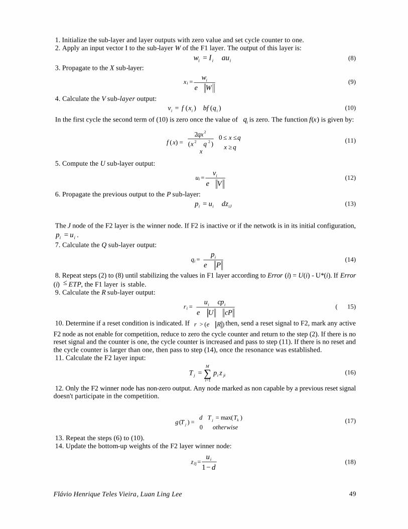
1. Initialize the sub-layer and layer outputs with zero value and set cycle counter to one. 2. Apply an input vector I to the sub-layer W of the F1 layer. The output of this layer is:

iii auIw += (8)

3. Propagate to the X sub-layer:

x i =We

wi

+ (9)

4. Calculate the V sub-layer output: )()( iii qbfxfv += (10)

In the first cycle the second term of (10) is zero once the value of iq is zero. The function f(x) is given by:

θθ

θθ

≥≤≤

+=x

x

xx

xxf

0)(

2)( 22

2

(11)

5. Compute the U sub-layer output:

ui =Ve

vi

+ (12)

6. Propagate the previous output to the P sub-layer:

iJii dzup += (13)

The J node of the F2 layer is the winner node. If F2 is inactive or if the netwotk is in its initial configuration,

ii up = . 7. Calculate the Q sub-layer output:

qi = Pe

pi

+ (14)

8. Repeat steps (2) to (8) until stabilizing the values in F1 layer according to Error (i) = U(i) - U*(i). If Error (i) ≤ ETP, the F1 layer is stable. 9. Calculate the R sub-layer output:

r i = cPUe

cpu ii

+++

( 15)

10. Determine if a reset condition is indicated. If )( Re +>ρ then, send a reset signal to F2, mark any active

F2 node as not enable for competition, reduce to zero the cycle counter and return to the step (2). If there is no reset signal and the counter is one, the cycle counter is increased and pass to step (11). If there is no reset and the cycle counter is larger than one, then pass to step (14), once the resonance was established. 11. Calculate the F2 layer input:

∑=

=M

ijiij zpT

1

(16)

12. Only the F2 winner node has non-zero output. Any node marked as non capable by a previous reset signal doesn't participate in the competition.

otherwise

TTdTg kj

j

)max(

0)(

=

= (17)

13. Repeat the steps (6) to (10). 14. Update the bottom-up weights of the F2 layer winner node:

zJj =d

u i

−1 (18)


15. Update the top-down weights of the F2 layer winner node:

ziJ =d

ui

−1 (19)

16. Remove input vector, restore inactive F2 nodes and return to the step (1) with a new input vector. 4 Recurrent Neural Networks

Artificial neural networks have been applied in the prediction and identification of time series [8][9]. A common neural network is made of individual units termed neurons. Each neuron has a weight associated with each input. A function of the weights and inputs (typically, a squashing function applied to the sum of the weight-input products) is then generated as an output. When neural networks are used to do sequence processing, the most general architecture is a recurrent neural network (that is, a neural network in which the output of some units is fed back as an input to some others), in which, for generality, unit outputs are allowed to take any real value in a given interval instead of simply two characteristic values as in threshold linear units. The growing interest in recurrent neural network is also due to its temporal processing and its capacity to implement adaptive memories [10]. Next, we describe the recurrent neural network type that composes the ART2/EKF architecture. Let a recurrent neural network consisting of N neurons with M external input, x(n) the input vector Mx1 in the time instant n, and y(n+1) the output vector Nx1 in the time instant n+1. We define the vector u(n) as a concatenation of two vectors x(n) and y(n). If Ai ∈ then )()( nxnu ii = , if Bi ∈ then )()( nynu ii = , where A the external input set, and B the output set. The considered recurrent neural network has two layers: a processing layer and input-output concatenation layer (Fig.3). The neural network is completely connected with MN direct connections, 2N feedback connections and z-1 is a unit delay applied to the output vector. We will call W the weight matrix with N(M+N) dimension. Let )(nv j be the j neuron internal activity in the time instant n for Bj ∈ :

∑∪∈

=BAi

ijij nunwnv )()()( (20)

where jiw represent synaptic weights. The j neuron output at the next instant is given by:

))(()1( nvny jj ϕ=+ (21)

Equations (20) and (21) describe the system dynamics where the functionϕ is assumed to be a linear ramp function.

Figure 3: Recurrent neural network.


5 An Extended Kalman Filter based Training Algorithm The Kalman filter consists of a group of equations that provide an efficient and recursive computation for the solution of the least squares method [11]. The EKF is a modification of the Linear Kalman Filter and can handle non-linear dynamics and non-linear measurement equations. The EKF is an optimal estimator that recursively combines noisy data with a model of the system dynamics. The Extended Kalman Filter (EKF) can be used as a real time algorithm for recurrent neural network weight determination. In this case, the real time learning is considered a filtering problem. Once the neural network is a non-linear structure, the extended Kalman filter is more adequate to train neural networks than the tradicional Kalman filter. Roughly speaking, the extended Kalman filter ‘linearizes’ the non-linear part of the system and it uses the original Kalman filter in this linearized model. The EKF algorithm was initially applied in the MLP neural network training by Singhal and Wu [12]. They showed that the EKF algorithm converges faster than the backpropagation algorithm and sometimes, when the backpropagation fails, the EKF (Extended Kalman Filter) converges for a good solution. Puskorius and Feldcamp applied the Kalman algorithm in the recurrent neural network training [13]. Williamns trained recurrent neural networks through the Extended Kalman Filter [14]. We address this training with a different state vector formulation. First, we present the equations of the Extended Kalman Filter used in this work. The extended Kalman filter estimates the vector sate )(ny at time instant n of a non-linear system described by the following equations:

)())(()( nrnxhny n += (22) )())(()1( nqnxfnx n +=+ (23)

where x(n+1) is the measure vector, r(n) represents the system noise and q(n) the measure error. Let )1\(ˆ −nnx be an ‘a priori’ estimate of the system state at time instant n given the knowledge of the measures until time instant n-1 and )\(ˆ nnx be ‘a posteriori’ estimate of the system state at time instant n given the knowledge of the measures until time instant n. The non-linear functions h and f can be written according to the Taylor expansion as:

....))1\(ˆ)()(())1\(ˆ())(( +−−+−= nnxnxnHnnxhnxh nnn (24)

....))\(ˆ)()(,1())\(ˆ())(( +−++= nnxnxnnFnnxfnxf nnn (25)

where the Jacobian matrixes ),1( nnFn + e )(nH n are given by:

xnnxf

nnF nn ∂

∂=+

)\(ˆ(),1( (26)

and

x

nnxhnH n

n ∂−∂

=)1\(ˆ(

)( (27)

Then, we can rewrite equations (22) and (23) as:

)()()()()( nrnunxnHny n ++= (28)

)()()(),1()1( nqnvnxnnFnx n +++=+ (29) where:

))1\(ˆ)())1\(ˆ()( −−−= nnxnHnnxhnu nn (30)

)\(ˆ),1())\(ˆ()( nnxnnFnnxfnv nn +−= (31) The derivatives corresponding to equations (26) and (27) are computed in each iteration, resulting in the following algorithm.

Kalman Gain computing:


)()()1\()()()1\(

)(nRnHnnPnH

nHnnPnK

Tnn

Tn

+−−

= (32)

Measure update equations: ))]1\(ˆ()()[()1\(ˆ)\(ˆ −−+−= nnxhnynKnnxnnx n (33)

)1\())()(()\( −−= nnPnHnKInnP n (34) Temporal update equations:

))\(ˆ()\1(ˆ nnxfnnx n=+ (35)

)(),1()\(),1()\1( nQnnFnnPnnFnnP Tnn +++=+ (36)

Now, we turn to the Extended Kalman Filter based neural training. Let d(n) be the desired output vector of size sx1. Our aim is to find the w(n) neural weights (system states) such that the difference among the neural network output and the desired be minimum in terms of quadratic error. The equations that govern the recurrent neural network operation are:

)())(),(()( nrnunwhnd n += (37)

)()1( nwnw =+ (38) where d(n) is viewed as the measurement vector, r(n) is the error measurement vector and the non-linear function nh describes the relationship among the input u(n) and the weights w(n). The EKF algorithm can be applied for the training of the previously presented recurrent neural network through the following equations:

Measurement Update Equations :

)()()1\()()()1\(

)(nRnHnnPnH

nHnnPnK

Tnn

Tn

+−−

= (39)

))](),1\(ˆ()()[()1\(ˆ)\(ˆ nunnwhndnKnnwnnw n −−+−= (40)

)1\())()(()\( −−= nnPnHnKInnP n (41)

Temporal Update Equations:

)\(ˆ)\1(ˆ nnwnnw =+ (42) )\()\1( nnPnnP =+ (43)

where:

wnunwh

nH nn ∂

∂=

))(),(ˆ()( (44)

and 1 2(.) [ , ,..., ]n sh h h h= are the s neural network outputs, R(n) is the measurement error covariance matrix,

P is the state error covariance matrix, )(ˆ nw is a state estimate (weights) and K(n) is known as Kalman gain [15]. 6 Application Example Real time traffic prediction is extremely useful for adaptive traffic flow control. Algorithms designed to make on line predictions are highly intended particularly when their prediction errors are similar to the on batch training of neural networks such as MLP and RBF ones [16].

The dynamic weight updating of the ART2/EKF neural architecture is suitable for signals that present

abrupt variations, such as traffic processes. Thus, we validate the prediction capacity of the proposed


ART2/EKF neural architecture through simulations with real network traffic traces collected from Bellcore1.

We also verify that the ART2/EKF neural architecture is capable of mapping l instants in the future points

with present points, i.e, it really predicts the volume of the traffic flows. Moreover, we applied the obtained

predictions in a dynamic rate allocation scheme for computer network links.

The prediction performance is usually evaluated through the normalized mean square error (NMSE)

given by [8][16]:

∑=

−=p

n

nynyp

NMSE1

22

)](ˆ)([1

σ (45)

where y(n) is the value of the time series, )(ˆ ny is the predicted value, 2σ is the real sequence variance on the

prediction interval and p is the number of test samples.

Some parameter values must be chosen in the ART2 neural network configuration. We set the following:

θ =0,3, ρ =0,9 and ETP=0,1. The ART2/EKF was applied in the prediction of the following traffic traces:

Bc-Octext trace with 2046 sample points at time scale of 1min and the Bc-Octint trace with 1759 points at

time scale of 1s.

Different time instants from the same traffic trace were used in the training and prediction by the neural

network architecture. In the Bc-Octint predicion, we obtain a NMSE equals to 0,3938 for the time instants 801

to 1701. This test is accomplished by using two recurrent neural network, two neurons for each neural net,

with five inputs equivalent to five points in sequence of the Bc-Octint traffic trace and a learning rate of 0,1.

Maintaining the same ART2/EKF configuration but using two input elements for the recurrent neural

networks, results in a NMSE of 0,4077 for the prediction of the points 1000 to 2000 for the Bc-Octext traffic

trace (Fig.4). Table 1 compares the NMSE of our proposal to the MLP and FIR MLP neural networks

trained with on batch methods. It can be noticed that the ART2/EKF achieves a smaller NMSE mainly for

the Bc-Octint traffic trace. This result is due to the distributed processing of the ART2/EKF. Since the

Bc-Octint trace has a strong statistical variation, the ART2/EKF takes advantage by creating different

categories (neural networks) to predict this traffic trace.

Time Series

MLP FIR- MLP

ART2/EKF

Bc-Octext 0,4077 0,4260 0,4057 Bc-Octint 1,21 0,7408 0,3938

Table 1: NMSE of prediction

1 http://ita.ee.lbl.gov/


Figure 4: One-step ahead prediction by the ART2/EKF architecture (solid line). Bc-Octext traffic trace

(dashed line).

The ART2/EKF prediction performance can be incorporated into a scheme that dynamically allocates the

rate that is necessary to avoid byte losses in a communication network link. The dynamic bandwidth

allocation scheme is shown in Fig. 5. In this scheme, the necessary bandwidth is estimated in advance which

permits that the network makes the change in the link rate, avoiding congestion before it happens. In our

simulation of this network link scenario, we used a sampling rate ∆ of 0,1s and a rate adaptation interval, i.e.,

a prediction step of M=4 ∆ . Therefore, the neural network directly has to map four time instant distant points.

In each time instant, we obtain fourth point ahead prediction 4)(nx̂ 1 + , 4)(nx̂ 2 + , 4)(nx̂ 3 + and 4)(nx̂ 4 + . The

allocated transmission rate tx for the following M seconds is given by:

4)}(nx̂ 4),(nx̂ 4),(nx̂ 4),(nx̂{maxtx 4321 ++++= (46)

Differently of [17][18], we do not use additional control gain to absorb non-well predicted sample points.

As traffic input for the single-buffer network link, we considered all the points of the Bc-Octint trace at the

time scale of 0.5s. Initially, we stipulated the number of bytes supported by the buffer as 70% of the Bc -Octint

trace maximum value. In the extended Kalman algorithm initialization, we set all weights with value 0,1 to

remove the random initial weigth choice. Besides, the R matrix was initialized with value 100 and the P

matrix with 800*800* I14x14 where I is the identity matrix.


Figure 5: Dynamic bandwidth allocation scheme.

The rate allocation scheme that uses the proposed neural architecture achieved a mean rate allocation of

355.840bytes/s. By allocating a static transmission rate equals the obtained mean rate allocation of

355.840bytes/s, it would have obtained a 3.439.800 byte loss. On the other hand, the dynamic rate allocation

provides a better performance, since 73.728 bytes are lost. Varying the buffer size while keeping the same

neural network and system configurations, we relate the byte loss and the maximum number of bytes that can

be stored in the buffer as shown in Fig.6.

0.5 0.6 0.7 0.8 0.9 1 1.1 1.2 1.30

0.5

1

1.5

2

2.5

3

3.5

4

4.5 x 106 Byte loss X Buffer size

B yte loss

mx bytes

Fig.6. Relationship between the byte loss and the buffer size for dynamic rate allocation (solid line) and for static transmission rate allocation (dashed line).

7 Conclusion In the ART2 mechanism, once a feature is deemed “irrelevant” in a given category, it will remain irrelevant throughout the future learning experiences of that category in that such a feature will never again be encoded into the LTM (Long Term Memory) of that category. Intuitively, a feature that is consistently present tracks the most recent amplitudes of that feature, eventually forgetting subtle differences of its past exemplars, much as encoding specificity effects and episodic memory. The proposed EKF based training algorithm is fast and provides excellent modeling performance for small recurrent neural network, i.e, neural networks possessing a few number of neurons. This characteristic is quite interesting because small recurrent neural networks can deal with different categories (patterns). In a similar way, the brain recognizes different visual patterns and the information is sent to different specialized areas


(not forgetting important patterns). The proposed ART2/EKF is a robust neural architecture that self organize in response to the inputs and it distributes its learning to different neural subnetworks maintaining what was already learned. We verified that this mechanism greatly enhance the prediction performance compared to other methods. Another interesting feature of the ART2/EKF is that its weights are updated in order to track the traffic statistical variations that can happen for which neural networks with on batch training could not be prepared. It can be noticed that a smaller byte loss is guaranteed by controlling the link rate through ART2/EKF predictions. An accentuated reduction was verified in the byte loss by applying the ART2/EKF based dynamic transmission rate allocation compared to a static allocation. According to the accomplished analysis, the proposed neural architecture is a useful tool for network traffic prediction and resource allocation. References [1] Carpenter, G. A. and Grossberg, S., Adaptive Resonance Theory. The Handbook of Brain Theory and

Neural Networks, Second Edition, MIT Press, 2003. [2] Levine, D. S., Introduction to Neural and Cognitive Modeling, Mahwah, New Jersey: Lawrence Erlbaum

Associates, Chapter 6, 2000. [3] Otwell, K., Incremental backpropagation learning from novelty-based orthogonalization, Proceedings of

the International Joint Conference on Neural Networks, Washington, DC, 1990. [4] Ryan, T. W. , The Ressonance Correlation Network, IEEE International Conference on Neural Networks,

pp.673 – 680, 24-27 July, 1988. [5] Carpenter, G.A. and Grossberg, S., ART2: Self-organization of stable category recognition codes for

analog input patterns, Applied Optics, 26 (23): 4919-4930, 1987. [6] Page, M., Connectionist modelling in psychology: a localist manifesto, Behavioral and Brain Sciences, 23,

pp. 443-512, 2000. [7] Pollen, D. A., On the neural correlates of visual perception, Cerebral Cortex, 9, pp.4-19, 1999. [8] Doulamis, A. D., Doulamis, N. D. and Kollias, S. D., An Adaptable Neural-Network Model for Recursive

Nonlinear Traffic Prediction and Modeling of MPEG Video Sources. IEEE Transactions on Neural Networks, 14(1), Jan. 2003.

[9] Qiu, L., Jiang, D. and Hanlen, L., Neural network prediction of radio propagation. Proceedings of Communications Theory Workshop, pp. 272 – 277, Feb. 2005.

[10] Bengio, Y., Frasconi, P. and Gori, M. Recurrent Neural Networks for Adaptive Temporal processing, Universitá di Firenze, Julho 1993;

[11] Zarchan, P. and Musoff, H., Fundamentals of Kalman Filtering: A Practical Approach. 2nd Edition, AIAA, 2005.

[12] Singhal, S. and Wu, L., Training multilayer perceptrons with the extended Kalman filter algorithm. Advances in Neural Information Processing Systems, 1989, pp. 133-140;

[13] Puskorius, G. V. and Feldkamp, L.A. Neurocontrol of nonlinear dynamical systems with Kalman filter trained recurrent networks, IEEE Transactions on Neural Networks, vol. 5, March, 1994, pp.279-297;

[14] Williamns, R. J. Training Recurrent Networks Using the Extended Kalman Filter. Technical Report . Boston: Northestern University, College of Computer Science, 1992;

[15] Haykin, S., Modern filters, Macmillan Publishing Company, 1989. [16] Vieira, F. H. T., Lemos, R. P. and Lee, L.L.. Aplicação de Redes Neurais RBF Treinadas com Algoritmo

ROLS e Análise Wavelet na Predição de Tráfego em Redes Ethernet. Proceedings of the VI Brazilian Conference on Neural Networks- pp.145-150, June 2-5, 2003 -SP- Brazil.

[17] Chong, S. and Li, S., Predictive dynamic bandwidth allocation for efficient transport of real-time VBR vídeo over ATM, IEEE JSAC, 13(1), Jan. 1995, pp.12-23;

[18] Vieira, F. H. T., Lemos, R. P. and Lee, L.L., Alocação Dinâmica de Taxa de Transmissão em Redes de Pacotes Utilizando Redes Neurais Recorrentes Treinadas com Algoritmos em Tempo Real. IEEE Latin America, 1, November 2003.

a neural architecture based on the adaptive … neural architecture based on the adaptive resonant...

Documents