a neural network approach for multi-attribute process …
TRANSCRIPT

A NEURAL NETWORK APPROACH FOR MULTI-ATTRIBUTE PROCESS CONTROL WITH COMPARISON OF TWO CURRENT TECHNIQUES AND
GUIDELEINES FOR PRACTICAL USE
by
Siripen Larpkiattaworn
B.S., Chemical Engineering, Chulalongkorn University, 1994
M.S., Industrial Engineering, University of Pittsburgh, 2000
Submitted to the Graduate Faculty of
School of Engineering in partial fulfillment
of the requirements for the degree of
Doctor of Philosophy
University of Pittsburgh
2003

UNIVERSITY OF PITTSBURGH
SCHOOL OF ENGINEERING
This dissertation was presented
by
Siripen Larpkiattaworn
It was defended on
June 17, 2003
and approved by
Jerrold H. May, Professor, Joseph M. Katz Graduate School of Business, University of Pittsburgh
Mainak Mazumdar, Professor, Industrial Engineering, University of Pittsburgh
Kim L. Needy, Associate Professor, Industrial Engineering, University of Pittsburgh
Harvey Wolfe, Professor, Industrial Engineering, University of Pittsburgh
Dissertation Director: Mary E. Besterfield-Sacre, Assistant Professor,
Industrial Engineering, University of Pittsburgh
ii

A NEURAL NETWORK APPROACH FOR MULTI-ATTRIBUTE PROCESS CONTROL WITH COMPARISON OF TWO CURRENT TECHNIQUES AND
GUIDELEINES FOR PRACTICAL USE.
Siripen Larpkiattaworn, Ph.D.
University of Pittsburgh, 2003
Both manufacturing and service industries deal with quality characteristics, which
include not only variables but attributes as well. In the area of Quality Control there has
been substantial research in the area of correlated variables (i.e. multivariate control
charts); however, little work has been done in the area of correlated attributes. To control
product or service quality of a multi-attribute process, several issues arise. A high number
of false alarms (Type I error) occur and the probability of not detecting defects increases
when the process is monitored by a set of uni-attribute control charts. Furthermore,
plotting and monitoring several uni-attribute control charts makes additional work for
quality personnel.
To date, a standard method for constructing a multi-attribute control chart has not
been fully evaluated. In this research, three different techniques for simultaneously
monitoring correlated process attributes have been compared: the normal approximation,
the multivariate np-chart (MNP chart), and a new proposed Neural Network technique.
The normal approximation is a technique of approximating multivariate binomial and

Poisson distributions as normal distributions. The multivariate np chart (MNP chart) is
base on traditional Shewhart control charts designed for multiple attribute processes.
Finally, a Backpropagation Neural Network technique has been developed for this
research. Each technique should be capable of identifying an out-of-control process while
considering all correlated attributes simultaneously.
To compare the three techniques an experiment was designed for two correlated
attributes. The experiment consisted of three levels of proportion nonconforming p, three
values of the correlation matrix, three sample sizes, and three magnitudes of shift of
proportion nonconforming in either the positive or negative direction. Each technique
was evaluated based on average run length and the number of replications of correctly
identified given the direction of shifts (positive or negative). The resulting performances
for all three techniques at their varied process conditions were presented and compared.
From this study, it has observed that no one technique outperforms the other two
techniques for all process conditions. In order to select a suitable technique, a user must
be knowledgeable about the nature of their process and understand the risks associated
with committing Type I and II errors. Guidelines for how to best select and use multi-
attribute process control techniques are provided.
iv

TABLE OF CONTENTS
1.0 INTRODUCTION....................................................................................................... 1
1.1 QUALITY CONTROL CHART APPLICATIONS................................................................ 1
1.2 BENEFITS OF MULTIVARIATE/MULTI-ATTRIBUTE PROCESS CONTROL VERSUS UNIVARIATE/UNI-ATTRIBUTE PROCESS CONTROL..................................................... 2
1.3 MULTI-ATTRIBUTE PROCESS QUALITY CONTROL APPROACHES................................ 3
1.4 RESEARCH OBJECTIVES.............................................................................................. 5
1.5 RESEARCH CONTRIBUTIONS....................................................................................... 5
2.0 LITERATURE REVIEW .......................................................................................... 7
2.1 UNI-ATTRIBUTE CONTROL CHARTS........................................................................... 8
2.1.1 Control Chart for Proportion Nonconforming (p-chart)................................... 9
2.1.2 Control Chart for Number of Nonconforming Items (np-chart) ........................ 9
2.1.3 Control Chart for the Number of Nonconformities (c-chart) .......................... 10
2.1.4 Control Chart for the Number of Nonconformities Per Unit (u-chart) ........... 10
2.1.5 Current Research Issues in Uni-Attribute Control Charts .............................. 11
2.2 MULTIVARIATE CONTROL CHARTS.......................................................................... 13
2.2.1 Hotelling T2 Control Chart .............................................................................. 14
2.2.2 Principal Component Analysis (PCA) ............................................................. 16
2.2.3 Partial Least Squares (PLS) ............................................................................ 18
2.3 MULTI-ATTRIBUTE CONTROL CHARTS .................................................................... 18
2.4 NEURAL NETWORKS AND CONTROL CHARTS .......................................................... 20
2.4.1 Neural Networks for Univariate Control Charts ............................................. 21

2.4.2 Neural Networks for Multivariate Statistical Process Control........................ 26
2.4.3 Neural Networks for Uni-Attribute Control Charts......................................... 26
2.4.4 Neural Networks for Multi-Attribute Control Charts ...................................... 27
2.5 INTERPRETATION OF OUT-OF-CONTROL SIGNALS FOR MULTIVARIATE CONTROL CHARTS.................................................................................................................... 27
3.0 MULTI-ATTRIBUTE METHODOLOGIES ........................................................ 30
3.1 CURRENT METHODS IN LITERATURE ....................................................................... 30
3.1.1 Normal Approximation of Multivariate Binomial Distribution ....................... 30
3.1.2 Multivariate np-Chart (MNP chart) ................................................................ 32
3.2 BACKPROPAGATION NEURAL NETWORKS................................................................ 34
3.2.1 General Concept .............................................................................................. 34
3.2.1.1 Architecture............................................................................................... 34
3.2.1.2 Algorithm.................................................................................................. 35
3.2.2 Backpropagation Neural Network for Multi-Attribute Process Control ......... 37
3.2.2.1 Architecture and Algorithm ...................................................................... 37
3.2.2.2 Preprocessing Data.................................................................................... 38
3.2.2.3 Training Data ............................................................................................ 39
3.2.2.4 Cut-Value for In-Control and Out-of-Control Processes.......................... 39
3.3 OTHER TECHNIQUES ................................................................................................ 40
3.3.1 Discriminant Analysis ...................................................................................... 41
3.3.2 Logistic Regression.......................................................................................... 42
3.3.3. Probabilistic Neural Network ......................................................................... 52
3.3.4 Cumulative Sum Control Procedures .............................................................. 55
4.0 EVALUATION OF METHODOGIES: EXPERIMENTAL DESIGN................ 57
4.1 DATA GENERATION ................................................................................................. 57
vi

4.2 THE EXPERIMENTAL DESIGN ................................................................................... 59
4.3 SAMPLE SIZES .......................................................................................................... 63
4.3.1 Sample Size #1 - Estimating Multivariate Normally Distributed Variables from a Multivariate Binomial Distribution ............................................................... 63
4.3.2 Sample Size #2 - Recommended Sample Size for the MNP Chart ................... 63
4.3.3 Sample Size #3 - Satisfying the Condition of Finding at Least One Non-Conforming Item in a Sample........................................................................... 64
4.4 LEVEL OF CORRELATION .......................................................................................... 65
4.5 NUMBER OF REPLICATIONS...................................................................................... 65
4.6 ASSUMPTIONS .......................................................................................................... 66
5.0 PERFORMANCE MEASURES.............................................................................. 67
5.1 AVERAGE RUN LENGTH (ARL) ............................................................................... 67
5.1.1 In-Control Average Run Length....................................................................... 68
5.1.2 Out-Of-Control Average Run Length............................................................... 68
5.2 PERCENTAGE OF CORRECT CLASSIFICATION............................................................ 68
6.0 MODEL VERIFICATION AND VALIDATION.................................................. 69
6.1 MODEL VERIFICATION ............................................................................................. 69
6.2 MODEL VALIDATION................................................................................................ 70
7.0 RESULTS AND ANALYSES .................................................................................. 72
7.1 SAMPLE SIZE #1 - ESTIMATING MULTIVARIATE NORMALLY DISTRIBUTED VARIABLES FROM A MULTIVARIATE BINOMIAL DISTRIBUTION................................ 72
7.1.1 p1 = 0.3, p2 = 0.3, Sample Sizes = 50 (Levels of Correlation: 0.8, 0.5, and 0.2).......................................................................................................................... 72
7.1.1.1 Comparing the BPNN to the Normal Approximation Techniques........... 74
7.1.1.2 Comparing the BPNN Technique to the MNP Chart................................ 77
7.1.1.3 Comparing the MNP Chart to the Normal Approximation Technique..... 78
vii

7.1.2 p1 = 0.1, p2 = 0.1, Sample Sizes = 100 (Levels of Correlation: 0.8, 0.5, and 0.2).................................................................................................................... 79
7.1.2.1 Comparing the BPNN to the Normal Approximation Techniques........... 80
7.1.2.2 Comparing the BPNN Technique to the MNP Chart................................ 83
7.1.2.3 Comparing the MNP Chart to the Normal Approximation Technique..... 85
7.1.3 p1 = 0.01, p2 = 0.01, Sample Sizes = 910 (Levels of Correlation: 0.8, 0.5, and 0.2).................................................................................................................... 85
7.1.3.1 Comparing the BPNN to the Normal Approximation Techniques........... 87
7.1.3.2 Comparing the BPNN Technique to the MNP Chart................................ 88
7.1.3.3 Comparing the MNP Chart to the Normal Approximation Technique..... 90
7.1.4 p1 = 0.3, p2 = 0.1, Sample Sizes = 100 (Levels of Correlation: 0.2)............... 91
7.1.4.1 Comparing the BPNN to the Normal Approximation Techniques........... 91
7.1.4.2 Comparing the BPNN Technique to the MNP Chart................................ 93
7.1.4.3 Comparing the MNP Chart to the Normal Approximation Technique..... 93
7.2 RECOMMENDED SAMPLE SIZE FOR THE MNP CHART .............................................. 94
7.2.1 p1 = 0.3, p2 = 0.3, Sample Sizes = 10 (Levels of Correlation: 0.8, 0.5, and 0.2).......................................................................................................................... 95
7.2.1.1 Comparing the BPNN to the Normal Approximation Techniques........... 98
7.2.1.2 Comparing the BPNN Technique to the MNP Chart.............................. 101
7.2.1.3 Comparing the MNP Chart to the Normal Approximation Technique... 102
7.2.2 p1 = 0.1, p2 = 0.1, Sample Sizes = 30 (Levels of Correlation: 0.8, 0.5, and 0.2)........................................................................................................................ 104
7.2.2.1 Comparing the BPNN to the Normal Approximation Techniques......... 107
7.2.2.2 Comparing the BPNN Technique to the MNP Chart.............................. 108
7.2.2.3 Comparing the MNP Chart to the Normal Approximation Technique... 110
viii

7.2.3 p1 = 0.01, p2 = 0.01, Sample Sizes = 810, 670, and 540 (Levels of Correlation: 0.8, 0.5, and 0.2)............................................................................................. 111
7.2.3.1 Comparing the BPNN to the Normal Approximation Techniques......... 113
7.2.3.2 Comparing the BPNN Technique to the MNP Chart.............................. 114
7.2.3.3 Comparing the MNP Chart to the Normal Approximation Technique... 116
7.3 SATISFYING THE CONDITION OF FINDING AT LEAST ONE NONCONFORMING ITEM IN A SAMPLE .................................................................................................................. 118
7.3.1 p1 = 0.3, p2 = 0.3, Sample Sizes = 10 (Levels of Correlation: 0.8, 0.5, and 0.2)........................................................................................................................ 118
7.3.2 p1 = 0.1, p2 = 0.1, Sample Sizes = 30 (Levels of Correlation: 0.8, 0.5, and 0.2)........................................................................................................................ 118
7.3.3 p1 = 0.01, p2 = 0.01, Sample Sizes = 300 (Levels of Correlation: 0.8, 0.5, and 0.2).................................................................................................................. 118
7.3.3.1 Comparing BPNN to the Normal Approximation Techniques............... 122
7.3.3.2 Comparing BPNN to the MNP Chart ..................................................... 123
7.3.3.3 Comparing the MNP Chart to the Normal Approximation Technique... 126
8.0 RECCOMENDATION FOR IMPLEMENTATION .......................................... 128
8.1 GUIDELINES FOR SELECTING A SUITABLE TECHNIQUE........................................... 141
8.2. GENERAL PERFORMANCES OF MULTI-ATTRIBUTE PROCESS CONTROL TECHNIQUES............................................................................................................................... 148
8.2.1 Normal Approximation Technique................................................................. 148
8.2.2 MNP Chart..................................................................................................... 149
8.2.3 Backpropagation Neural Network Technique ............................................... 150
8.3 INTERPRETATION OF OUT-OF-CONTROL SIGNALS.................................................. 150
9.0 CONCLUSIONS, CONTRIBUTIONS, FUTURE WORK................................. 152
APPENDIX A................................................................................................................ 157
APPENDIX B ................................................................................................................ 164
ix

LIST OF TABLES
Table 1 In-control ARL of the MNP chart, the normal approximation, and the
multinomial logistic regression techniques where the number of in-control and out-of-control observations in training set are equal .......................................... 46
Table 2 In-control ARL of the MNP chart, the normal approximation, the multinomial logistic regression techniques when number of in-control and out-of-control observations in training set are unequal: 500 in-control observations and 200 out-of-control observations (100 each for positive and negative direction of shifts). ................................................................................................................. 49
Table 3 In-control ARL of the MNP chart, the normal approximation, and the multinomial logistic regression techniques when number of in-control and out-of-control observations in training set are unequal: 10,000 in-control observations and 200 out-of-control observations (100 each for positive and negative direction of shifts). ............................................................................... 50
Table 4 Out-of-control ARL of the MNP chart, the normal approximation, and the multinomial logistic regression techniques when number of in-control and out-of-control observations in training set are unequal: 10,000 in-control observations and 200 out-of-control observations (100 each for positive and negative direction of shifts). ............................................................................... 51
Table 5 Experimental Design of Two Positively Correlated Attributes ........................... 61
Table 6 Performance of the Three Techniques for Experimantal Subset: p1=0.3, p2=0.3, Sample Sizes=50, Correlation Coefficient=0.8 .................................................. 73
Table 7 Performance of the Three Techniques for Experimental Subset: p =0.3,p =0.3, Sample Sizes=50, Correlation Coefficient=0.5
1 2.................................................. 74
Table 8 Performance of the Three Techniques for Experimental Subset: p1=0.3, p2=0.3, Sample Sizes=50, Correlation Coefficient=0.2 .................................................. 74
Table 9 Performance of the Three Techniques for Experimental Subset: p1=0.1, p2=0.1, Sample Sizes=100, Correlation Coefficient=0.8 ................................................ 79
Table 10 Performance of the Three Techniques for Experimental Subset: p1=0.1, p2=0.1, Sample Sizes=100, Correlation Coefficient=0.5 ................................................ 80
x

Table 11 Performance of the Three Techniques for Experimental Subset: p1=0.1, p2=0.1, Sample Sizes=100, Correlation Coefficient=0.2 ................................................ 80
Table 12 Performance of the Three Techniques for Experimental Subset: p =0.01, p =0.01, Sample Sizes=910, Correlation Coefficient=0.8
1
2 ................................. 86
Table 13 Performance of the Three Techniques for Experimental Subset: p =0.01, p =0.01, Sample Sizes=910, Correlation Coefficient=0.5
1
2 ................................. 86
Table 14 Performance of the Three Techniques for Experimental Subset: p =0.01, p =0.01, Sample Sizes=910, Correlation Coefficient=0.2
1
2 ................................. 87
Table 15 Performance of the Three Techniques for Experimental Subset: p1=0.3, p2=0.1, Sample Sizes=100, Correlation Coefficient=0.2 ................................................ 91
Table 16 Performance of the BPNN and the Normal Approximation Techniques for Experimental Subset: p1=0.3, p2=0.3, Sample Sizes=10, Correlation Coefficient=0.8................................................................................................... 95
Table 17 Performance of the BPNN Technique and the MNP Chart for Experimental Subset: p1=0.3, p2=0.3, Sample Sizes=10, Correlation Coefficient=0.8 ............ 96
Table 18 Performance of the BPNN and the Normal Approximation Techniques for Experimental Subset: p1=0.3, p2=0.3, Sample Sizes=10, Correlation Coefficient=0.5................................................................................................... 96
Table 19 Performance of the BPNN Technique and the MNP Chart for Experimental Subset: p1=0.3, p2=0.3, Sample Sizes=10, Correlation Coefficient=0.5 ............ 97
Table 20 Performance of the BPNN and the Normal Approximation Techniques for Experimental Subset: p1=0.3, p2=0.3, Sample Sizes=10, Correlation Coefficient=0.2................................................................................................... 97
Table 21 Performance of the BPNN Technique and the MNP Chart for Experimental Subset: p1=0.3, p2=0.3, Sample Sizes=10, Correlation Coefficient=0.2 ............ 97
Table 22 Performance of the BPNN and the Normal Approximation Techniques for Experimental Subset: p1=0.1, p2=0.1, Sample Sizes=30, Correlation Coefficient=0.8................................................................................................. 105
Table 23 Performance of the BPNN Technique and the MNP Chart for Experimental Subset: p1=0.1, p2=0.1, Sample Sizes=30, Correlation Coefficient=0.8 .......... 105
Table 24 Performance of the BPNN and the Normal Approximation Techniques for Experimental Subset: p1=0.1, p2=0.1, Sample Sizes=30, Correlation Coefficient=0.5................................................................................................. 105
xi

Table 25 Performance of the BPNN Technique and the MNP Chart for Experimental Subset: p1=0.1, p2=0.1, Sample Sizes=30, Correlation Coefficient=0.5 .......... 106
Table 26 Performance of the BPNN and the Normal Approximation Techniques for Experimental Subset: p1=0.1, p2=0.1, Sample Sizes=30, Correlation Coefficient=0.2................................................................................................. 106
Table 27 Performance of the BPNN Technique and the MNP Chart for Experimental Subset: p1=0.1, p2=0.1, Sample Sizes=30, Correlation Coefficient=0.2 .......... 106
Table 28 Performance of the Three Techniques for Experimental Subset: p =0.01, p =0.01, Sample Sizes=810, Correlation Coefficient=0.8
1
2 ............................... 112
Table 29 Performance of the Three Techniques for Experimental Subset: p =0.01, p =0.01, Sample Sizes=670, Correlation Coefficient=0.5
1
2 ............................... 112
Table 30 Performance of the Three Techniques for Experimental Subset: p =0.01, p =0.01, Sample Sizes=540, Correlation Coefficient=0.2
1
2 ............................... 113
Table 31 Performance of the BPNN and the Normal Approximation Techniques for Experimental Subset: p1=0.01, p2=0.01, Sample Sizes=300, Correlation Coefficient=0.8................................................................................................. 119
Table 32 Performance of the BPNN Technique and the MNP Chart for Experimental Subset: p1=0.01, p2=0.01, Sample Sizes=300, Correlation Coefficient=0.8 .... 120
Table 33 Performance of the BPNN and the Normal Approximation Techniques for Experimental Subset: p1=0.01, p2=0.01, Sample Sizes=300, Correlation Coefficient=0.5................................................................................................. 120
Table 34 Performance of the BPNN Technique and the MNP Chart for Experimental Subset: p1=0.01, p2=0.01, Sample Sizes=300, Correlation Coefficient=0.5 .... 121
Table 35 Performance of the BPNN and the Normal Approximation Techniques for Experimental Subset: p1=0.01, p2=0.01, Sample Sizes=300, Correlation Coefficient=0.2................................................................................................. 121
Table 36 Performance of the BPNN Technique and the MNP Chart for Experimental Subset: p1=0.01, p2=0.01, Sample Sizes=300, Correlation Coefficient=0.2 .... 121
Table 37 Comparisons of the BPNN and Normal Approximation Techniques for Large Sample Sizes..................................................................................................... 128
Table 38 Comparisons of the BPNN Technique and the MNP chart for Large Sample Sizes.................................................................................................................. 129
Table 39 Comparisons of the MNP Chart and the Normal Approximation Technique for Large Sample Sizes. ......................................................................................... 129
xii

Table 40 Meaning of Superscripts Used in the Comparisons between the BPNN technique and the MNP Chart. ......................................................................... 132
Table 41 The BPNN, MNP Chart and the Normal Approximation Technique for Large Sample Sizes. (Best performing techniques in each situation are shown by their first letters)........................................................................................................ 133
Table 42 Comparisons of the BPNN and Normal Approximation Techniques for the MNP Chart Sample Sizes. ................................................................................ 134
Table 43 Comparisons of the BPNN Technique and the MNP chart for the MNP Chart Sample Sizes..................................................................................................... 134
Table 44 Comparisons of the MNP chart and the Normal Approximation Technique for the MNP Chart Sample Sizes. .......................................................................... 135
Table 45 Comparisons of the BPNN and Normal Approximation Techniques for the Small Sample Sizes. ......................................................................................... 138
Table 46 Comparisons of the BPNN Technique and the MNP chart for the Small Sample Sizes.................................................................................................................. 138
Table 47 Comparisons of the MNP chart and the Normal Approximation Technique for the Small Sample Sizes. ................................................................................... 139
xiii

LIST OF FIGURES
Figure 1 Backpropagation Neural Network with One Hidden Layer ............................... 35
Figure 2 Back Propagation Neural Network Architecture................................................ 38
Figure 3 Probabilistic Neural Network Architecture For Two Categories ....................... 53
Figure 4 Ong’s Algorithm for Positive Correlation (0 < xyρ ≤ 1) .................................. 58
Figure 5 Ong’s Algorithm for Negative Correlation ( )01 <≤− xyρ ............................... 58
Figure 6 Procedure Used to Determine Number of Replications ..................................... 66
Figure 7 Confidence Regions of Normal Approximated Variables.................................. 77
Figure 8 Decision tree diagram for process with limited knowledge ............................. 147
Figure 9 Performances of the normal approximation technique with different correlation coefficient ......................................................................................................... 149
xiv
1.0 INTRODUCTION
Quality has been a concern in the manufacturing industry since 17001. In present
day, not only manufacturing but also service industries focus on product and service
quality as main factors for customer satisfaction. To be competitive in the market,
organizations must improve or at least maintain their product and service quality.
Control charts, which are effective tools to monitor final product and process quality
characteristics, were initially developed in 19242. Since then, several kinds of control
charts have been developed for different applications.
This research focuses on a relatively new area in quality control, namely that of
the development and evaluation of multi-attribute control charts.
1.1 Quality Control Chart Applications
Quality control charts can be applied to almost any area within a company or
organization, including manufacturing, process development, engineering design, finance
and accounting, marketing and field service. Shewhart X , S and R control charts are
extensively used to monitor continuous process variables. For example, a steel sheet
manufacturer considers sheet thickness as a major quality characteristic and monitors it
via Shewhart control charts. However, there are many situations in which more than one
variable is considered simultaneously. For instance, a bearing has inner and outer
diameters to determine the part quality. As a second example, the operating temperature
1

and pressure of a distillation column both affect the process yield. As an additional
example, Jackson3 presented the application of multivariate quality control in ballistic
missile and photographic film examples.
In addition to the continuous type of quality characteristics mentioned, there is
another data type of quality characteristic commonly referred to as discrete (or attribute
data). For example, a rod diameter is measured as “go” or “no-go” (i.e. the diameter
specification is given a “pass” or “do not pass”). Control charts constructed for discrete
data are called attribute control charts. Examples of processes that apply attribute control
charts include order taking (an example from the service sector) and integrated circuit
board fabrication (an example from manufacturing). For the order taking example, the
number of wrong orders taken is the attribute of interest, while in the integrated circuit
board fabrication example the number of defects on a wafer is monitored. Similar to
variable processes, attribute processes may involve more than one attribute. Many
service industries work with multiple attributes to describe their quality characteristics.
For instance, an airline company measures customer satisfaction as a function of the
mannerisms of the flight attendants and the overall flight time. A healthcare provider may
evaluate its performance by the number of service errors, and the number of negative
comments received about doctors, nurses, and overall service.
1.2 Benefits of Multivariate/Multi-Attribute Process Control versus Univariate/Uni-Attribute Process Control
When a process involves more than one variable, two different types of control
chart approaches can be selected, a single multivariate control chart or a set of univariate
control charts. A multivariate control chart is more sensitive and economical than a set of
2

univariate control charts. The number of false alarms (Type I error) decreases when a
multivariate control chart replaces a set of univariate control charts. In addition, a
multivariate chart shows out-of-control signals due to the joint effect of two or more
correlated variables; however, a set of univariate control charts may not show any such
signal because their individual effect may not be out-of-control. Lowry and Montgomery4
have shown that, in general, a multivariate control chart has better sensitivity than a set of
univariate control charts in monitoring multivariate quality processes. A multivariate
control chart is easier to use than maintaining numerous univariate control charts since
identifying an out-of-control sample in a multivariate control chart requires only one
observation versus many in univariate control charts. Equivalently, monitoring
simultaneous attributes via multi-attribute charts has similar benefits over monitoring
several single attributes at one time.
1.3 Multi-Attribute Process Quality Control Approaches
When developing a control chart technique for multi-attributes, the following
questions/statements should be considered. These questions/statements are adapted from
multivariate quality control goals given by Jackson5.
1. A single answer should be available to answer the question: “Is the process in
control?”
2. An overall Type I error should be specified.
3. Techniques should take into account the relationships among the attributes.
4. Techniques should be available to answer the question: “If the process is out-
of-control, what is the problem attribute?”.
3

As service industries, which most often involve the use of attribute data,
implement or improve upon quality programs, it has been found that control charts are
the most common tools utilized6. As a result, the demand for effective techniques to
monitor a process with multiple attributes simultaneously is increasing. However, little
research has been done in this area. From the literature only three studies have been
conducted; the first two studies focus on the statistical design of multi-attribute charts,
and the third study focuses on the economic design. The two statistical design techniques
are authored by Patel7 and Lu et al.8. Patel suggests a multivariate normal approximation
technique for multivariate binomial and Poisson distributed data. Lu et al. develop a
multivariate np-chart (MNP chart) based on a Shewhart-type control chart to deal with
multiple attribute processes. The economic design study is conducted by Jolayemi9. In his
work, Jolayemi develops a J approximation technique to approximate the sum of
independent binomial distributions, which have different proportion nonconforming.
The multi-attribute research mentioned specifies the probability of falsely
identifying an in-control sample; however, neither author discusses how fast the control
charts can detect an out-of-control sample. Lu et al. show that multivariate np-chart is
more sensitive than a set of uni-attribute control charts but their conclusion is based on
only a single numerical example. The literature lacks any discussion about how well the
current multi-attribute process control techniques work on various values of proportion
nonconforming, different magnitudes of mean(s) shift (shift of proportion
nonconforming), and different values of the correlation matrix.
4

1.4 Research Objectives
The objective of this research is two-fold. The first objective is to develop a
technique for monitoring a multi-attribute process. The proposed technique meets the
objectives of stated in section 1.3, as well as requires smaller sample sizes than the
current techniques described. This new technique is based on the use of backpropagation
neural networks (BPNN), which has had many successes in the quality control arena. The
second objective of this research is to conduct a comparison study among the two current
statistical approaches (normal approximation and MNP chart) and the proposed neural
network technique given different conditions of proportion nonconforming p, sample size
n, correlation matrix, and direction and magnitude of mean(s) shift (shift of process’s
proportion nonconforming). Out-of-control average run length (ARL) and in-control
ARL will be used as performance measures for the three comparisons. The number of
replications of correctly identified directions of shifts (positive or negative) will be also
considered in the performance comparison.
As a result of this research, guidelines have been developed for quality control
engineers and administrators who intend to monitor their multiple attribute processes.
Based on the guidelines, users can more easily select the most promising technique to
satisfy their particular process conditions.
1.5 Research Contributions
From this research, a new technique using backpropagation neural network
(BPNN) for monitoring multi-attribute processes has been developed and successfully
evaluated. This technique is preferable for processes with small sample size. In addition,
5

the new technique is able to identify the directions of shifts and this quality narrows
down causes of the shifts. This research also presents how the current and proposed
multi-attribute process control techniques perform in different process conditions.
Finally, guidelines and benefits of using a particular technique versus the others are
provided for particular users.
This document is organized in the following manner. Chapter 2 includes the
literature review. Chapter 3 explains the various multi-attribute methodologies that were
investigated. These include the above mentioned techniques as well as an investigation
of other possible techniques. Chapter 4 provides an overview of the experimental design
used to compare the three techniques and Chapter 5 discusses the performance measures
used in the experiment. Chapter 6 describes how the code used to test the three
techniques was verified and how the data generated for the experiment were validated.
Chapter 7 provides the results of the experiment. Chapter 8 recommends how one might
determine the best technique to employ given particular process conditions. Finally,
Chapter 9 gives conclusions and contributions, and suggests directions for future research
in the area of multi-attribute control charts.
6

2.0 LITERATURE REVIEW
Control charts have been used as tools for monitoring industrial and service
related processes for decades. In general, control charts can be categorized into two
groups by the type of quality characteristic. A quality characteristic, which is measured
on a numerical scale, is called a variable. X , S and R charts are broadly used to monitor
the mean and variability of variables. However, not all quality characteristics can be
measured numerically. This type of quality characteristic classifies an inspected item as
either conforming or nonconforming to a particular specification. The latter quality
characteristic is called an attribute. In the same manner, p, np, c and u-charts are
extensively used to observe attribute means.
Depending on the nature of the process, either variable or attribute control charts
may be used. Based on the needs of the customer, engineers select the type of control
chart. Montgomery10 suggests criteria for choosing the proper type of control chart.
Advantages and disadvantages of attributes vs. variable control chart are also
recommended11. Below are some advantages for using attributes control charts.
Attribute control charts can provide joint quality characteristics, e.g. height,
length and width, in one chart. Products are defined as nonconforming when any
one characteristic fails to meet specifications. On the other hand, three separate
variable control charts are needed if we consider the quality characteristics as
variables.
7

Attributes control charts consume less time and cost in inspection than variable
control charts.
Disadvantages of attribute control charts include, but are not limited to, the following.
Variable control charts can forewarn operators when the process is about to go
out-of-control so that actions can be taken before any nonconforming products are
actually produced. In contrast, attribute control charts will not indicate any such
signal until the nonconforming products are produced.
Attribute control charts require larger sample sizes than do variable controls
charts to indicate a process shift.
Attribute information does not provide potential causes; therefore remedial
actions cannot be identified.
This literature review discusses various types of uni-attribute, multivariate control
charts and current multi-attribute process control techniques. The last section of this
Chapter presents neural network applications for control charts.
2.1 Uni-Attribute Control Charts
In addition to applications of attribute control charts in manufacturing processes,
attribute control charts are very useful in service industries. One reason for the wide use
of attribute control charts in service industries is that most of the quality characteristics
are measured on a quality scale such as satisfied or unsatisfied. Palm et al. discussed
control chart applications in relatively new areas such as the service industry12. Health
care providers have applied attribute control charts to measure service quality and
expense. Educational institutions are also one of latest areas in which attribute control
8

charts are being implemented.13 Several types of attribute control charts will be discussed
next.
2.1.1 Control Chart for Proportion Nonconforming (p-chart)
The p-chart is used to monitor the proportion nonconforming. The proportion
nonconforming is the ratio of number of nonconforming items in a population to the total
number of items in the population. In service industries, the proportion nonconforming
may be the ratio of number of unsatisfied customers to the total number of customers.
The upper and lower control limits and centerline are calculated as follows.
)/)1((3 npppitsControlLim −±= , (2-1)
pCenterline = , (2-2)
where p and n are the proportion nonconforming and sample size respectively. The
statistic p estimates p when p is unknown.
2.1.2 Control Chart for Number of Nonconforming Items (np-chart)
For the p-chart, operators convert the number of nonconforming items in the
sample to proportion nonconforming. The conversion process can be discarded by
switching to np-charts since numbers of nonconforming items from samples are plotted
instead of the proportion nonconforming. There is one drawback in the np-chart. The
control limits and centerline will change when the sample size varies. Control limits and
centerline formulas are given below.
)1(3 pnpnpitsControlLim −±= , (2-3)
9

npCenterline = , (2-4)
where p and n are the proportion nonconforming and sample size respectively.
2.1.3 Control Chart for the Number of Nonconformities (c-chart)
A c-chart is used when the number of defects or nonconformity in an item is of
particular concern, such as the number of defective welds in 10 meters of oil pipeline, the
number of defects in 100 m2 of fabric, etc. In constructing a c-chart, the size of sample is
called the area of opportunity. The area of opportunity may consist of a single unit or
multiple units of an item. A constant size area of opportunity is required when c-chart is
constructed. This control chart assumes that the underlying distribution of the occurrence
of the nonconformities in a sample of constant size is Poisson. The centerline and control
limits are given below.
ccitsControlLim 3±= , (2-5)
cCenterline = , (2-6)
where c is the average number of nonconformity in an area of opportunity.
2.1.4 Control Chart for the Number of Nonconformities Per Unit (u-chart)
A c-chart is used when the sample size is constant. If the sample size changes
from one sample to another, a u-chart is the proper tool. Even though the u-chart control
limits change when sample size varies, the centerline remains constant. The centerline is
the average number of nonconformities per unit.
∑∑==
i
i
nc
uCenterline , (2-7)
10

where ci and ni are the number of nonconformities and sample size of the ith sample.
The control limits are given by the following equation.
)/(3 nuuitsControlLim ±= (2-8)
2.1.5 Current Research Issues in Uni-Attribute Control Charts
A primary issue of discussion in attribute control charts is the appropriate sample
size. The sample size should be selected to ensure that the normality assumption is not
violated.14 In the p and np-charts, when the proportion nonconforming is very small,
sample size must be large. However, too large of a sample size causes a problem for a
process with limited resources. Schwertman and Ryan suggest an alternative procedure
called dual np-charts.15 Dual np-charts are composed of two charts. One chart provides an
early warning of quality deterioration and the other, a cumulative control chart, uses
approximate normal theory properties. The first chart has a smaller sample size than the
second chart. As a result, the control limits for the two charts are different.
Chen also discusses the use of large sample sizes, but adds information about the
speed of detecting a shift in the mean.16 In the p-chart, the lower control limit is always
close to “0”, which makes the probability of detecting decreases in p small. In order to
have effective lower control limits, large samples sizes are required. Chen suggests two
alternative charts, which are based on discrete probability integral transformations and
arcsine transformations, respectively. He compared the alternative charts with the
classical p-chart using three criteria: (1) the minimum sample size for effective lower
control limits, (2) the closeness of the false alarm probabilities to the nominal values for
11

both upper and lower control limits, and (3) the ability to detect a change in p right after
the change occurs.
How fast a control chart detects the p shift, especially when the p shift is small, is
another issue that has been discussed by several authors. The CUSUM chart is an
alternative to the classical Shewhart p-chart. Reynolds and Stoumbos17 developed two
CUSUM charts. One chart is based on the binomial distribution in which variables are
counted from the number of defective items in n sample size. The second chart is based
on Bernoulli variables resulting from inspections of the individual items. Both CUSUM
charts are faster in detecting small shifts in p than traditional Shewhart p-charts. Further,
CUSUM charts are better than p-charts for detecting large shifts in p. In addition,
Reynolds and Stoumbos provide the Sequential Probability Ratio Test (SPRT) chart,
which provides faster detection of changes in p than CUSUM and classical p-charts; and
the SPRT chart requires smaller sample sizes than CUSUM and classical p-charts in
order to detect changes.18 For processes where p is very small, such as parts-per-million,
Nelson19 introduces a new control chart as an alternative to the traditional p and c-charts
in order to avoid a large sample size. The number of conforming items between two
consecutive nonconforming items is counted, and is assumed to have an exponential
distribution. A transformation is then applied to the exponential distribution to
approximate a normal distribution.
For the c-chart, one of the interesting issues discussed in the literature is that the
distribution is assumed Poisson. There are situations in which the occurrence of defects in
an item of a process does not follow the Poisson distribution. For example, defects in
integrated circuit board fabrication are often clustered such that they do not follow a
12

Poisson distribution. Therefore, using a c-chart results in more false alarms. Two
methods, a Neyman-based control chart (a control chart on the Neyman-type A
distribution) and fuzzy ART, are suggested by Su and Tong20. The Neyman-type A
distribution is a member of the family of compound Poisson distributions. One drawback
of the Neyman-based control chart is that it cannot be applied to large sample sizes.
2.2 Multivariate Control Charts
In most processes, more than one quality characteristic can affect the final product
quality. In another words, multiple quality characteristics are monitored simultaneously.
In such cases, engineers develop and monitor either several univariate control charts or a
single multivariate control chart. The practice is similar for attribute control charts. One
drawback of using several univariate control charts is that the probability of a Type I
error (plotting the sample outside control limits when it is really in control) increases. An
increased Type I error will result in a higher number of false alarms to occur. For
example, consider a process that consists of two independent quality characteristics, x1
and x2, each plotted on separate control charts. Each individual chart has Type I error of
0.0027 given three sigma control limits. Assuming independence, the joint probability of
plotting the sample in control limits when it is actually in control is (1-.0027)(1-.0027) =
0.9946. The overall Type I error of the two univariate control charts is 1- 0.9946 =
0.0054, which is two times larger than the 0.0027 Type I error of a single multivariate
control chart. Therefore, if we have two independent quality characteristics and would
like to maintain an overall Type I error of 0.0027, each individual chart Type I error
needs to be adjusted to 0.001351. Consider the example where 10 variables are
13

investigated instead of two. Type I error will increase to 0.026 (roughly a 10 times
increase). As the number of quality characteristics increases the Type I error distortion
becomes more severe.
If the quality characteristics are not independent, a more complex process must be
employed to obtain the overall Type I error. Aparisi21 provides control limits when the
two variables, x1 and x2, follow a bivariate normal distribution. Using a multivariate
control chart reduces the operating personnel’s work by plotting only one chart instead of
multiple charts. In addition, monitoring the process status in multivariate control charts is
easier than univariate control charts. However, assignable causes of an out-of-control
process are more easily defined by set of univariate control charts.
There are several standard statistical process control methods that can be used to
monitor the processes with multiple variables, such as the Hotelling T2 control chart,
Principal Component Analysis (PCA), Partial Least Square (PLS), to name a few. The
three techniques mentioned will be discussed.
2.2.1 Hotelling T2 Control Chart
Hotelling22 conducted the original work in multivariate control charts. The
Hotelling T2 control chart was developed to monitor process variables simultaneously and
overcome the drawbacks associated with using several univariate control charts when
variables are correlated. The underlying distribution of the quality characteristics for
which the Hotelling T2 is appropriate is multivariate normal; however, a small deviation
from multivariate normal distribution will not affect the results severely. The procedure
for constructing the control chart is similar in nature to other types of control charts. The
14

procedure is composed of two phases. The objective of phase I is to obtain an in-control
set of observations so that control limits can be established for phase II. Phase II uses the
control chart derived in phase I to monitor whether the future process is in-control or not.
Historical or new data (preliminary) collected from the process is used to generate a
phase I control chart. A sample mean and variance are estimated. Samples that are shown
to be out-of-control are investigated and deleted from the data set if assignable causes are
found. A new control chart without these points is then developed. The estimated mean
vector and covariance matrix are:
∑=
=m
kjkj X
mX
1
1 j = 1, 2, …, υ and k = 1, 2, …, m (2-9)
∑=
=n
iijkjk X
nX
1
1 i = 1, 2, …, n (2-10)
∑=
=m
kjkj S
mS
1
22 1 j = 1, 2, …, υ and k = 1, 2, …, m (2-11)
∑=
=m
kjhkjh S
mS
1
1 j≠ h (2-12)
where m is the number of samples collected for preliminary data, υ is the number of
monitored variables and n is the sample size. The test statistic is given as
)()'( 12 xxSxxnT −−= − . (2-13)
In phase I, control limits for T2 control chart are
1,,1)1)(1(
+−−+−−−−
= υυαυυ
mmnFmmn
nmolLimitUpperContr , (2-14)
0=olLimitLowerContr . (2-15)
where α is a specified significance level and F is F distribution. Once the chart is used
for monitoring future observations (Phase II), the control limits are
15

1,,1)1)(1(
+−−+−−−+
= υυαυυ
mmnFmmn
nmolLimitUpperContr , (2-16)
0=olLimitLowerContr . (2-17)
The Chi-square distribution with υ degrees of freedom, where υ is the number of
variables, and a significance level of α can be used as the upper control limits for both
phase I and II when the mean vector, variance and covariance matrix are estimated from a
large number of preliminary samples.23
2.2.2 Principal Component Analysis (PCA)
Principal Component Analysis is a useful technique for multivariate statistical
process control, particularly with large size data and correlated variables. The general
concept of PCA is to reduce a data matrix’s dimension from m to k (k<m). The reduced
dimensional matrix accounts for the majority of variability in the original data. Principal
Component Analysis calculates a vector, called the first principal component, which is a
linear combination of the m measure variables. This line is the direction of maximum
variance and is defined so as to minimize the orthogonal deviation from each data point.
A unit vector, which defines the direction of a principal component, is called an
eigenvector. The distance of each original data point, which is projected along ith
principal component, is called a z-score (zi). The second component is obtained in the
same way as the first principal component but it is fitted through the residual variation of
the first component. Both the first and second components are orthogonal. This approach
is continued until m principal components, which are orthogonal, are obtained. For large
16

data sets, it is often found that the first k components (k << m) explain the majority of the
variation in the data matrix.
According to Jackson24, Principal Component Analysis (PCA) can be useful in
multivariate process quality control because it transforms a set of correlated variables to a
new set of uncorrelated variables. Quality engineers can then plot individual control
charts from the sets of uncorrelated variables. However, Type I error is increased when
variables are monitored individually. Techniques, such as Hotelling T2, can take care of
this increased Type I error. From Jackson25,
, (2-18) yyT '2 =
, (2-19) ⎥⎥⎥⎥
⎦
⎤
⎢⎢⎢⎢
⎣
⎡
=
k
i
y
yy
y:
1
iii lzy /= , (2-20)
where zi is projected distance along ith principal component of each original data point.
The variance of zi is eigenvalue li. A process is out of control if T2 is larger than upper
control limit where
( )αυυυ
υ,,
1−−
−= mF
mmolLimitUpperContr , (2-21)
0=olLimitLowerContr , (2-22)
and F is the F distribution.
If the process is out of control, yi must be examined to provide the root causes of
the out-of-control condition. One advantage of using PCA is that quality engineers only
have to work with k instead of m variables (k<m).
17

2.2.3 Partial Least Squares (PLS)
Often one group of variables, Y, is of great importance, such as product quality,
and should be included in the monitoring process. Unfortunately, these variables are
measured much less frequently and accurately than the normal process variables, such as
X. Therefore, a technique using process variables, X, to detect and predict the change of
product quality variables, Y, is used. This technique, Partial Least Squares (PLS), is a
regression method based on projecting a high dimensional space (X,Y) onto a lower
dimensional space defined by two sets of latent variables from both X and Y. Wold26
provides details on the use of PLS.
2.3 Multi-Attribute Control Charts
Multi-attribute control charts can be used to simultaneously monitor many
attribute quality characteristics of a process. The objectives of multi-attribute control
charts are the same as multivariate control charts. Examples of industries that can
capitalize on the multi-attribute control charts are the airline, healthcare, and food service
industries. An airline company may measure customer satisfaction as a function of the
mannerisms of the stewards/stewardesses and the overall flight time. For a restaurant, the
food quality and the waiter’s behaviors are possible quality attributes.
Even though multi-attribute control charts can be as useful as multivariate control
charts, little research has been published. Patel conducted one of the earliest multi-
attribute control charts studies27. Patel developed quality control methods for multivariate
binomial and multivariate Poisson distribution observations. The correlated attributes
were monitored simultaneously. In addition, his work considered time-dependent
18

samples. Two assumptions, normality and equal process variance, are drawbacks of
Patel’s method. Lu et al.28 addressed the statistical design of multi-attribute control
charts. This paper discussed a mechanism for developing a Shewhart-based control chart
to deal with multiple attribute processes. The chart is called multivariate np-chart (MNP
chart). The MNP chart is easy to implement and interpret. An X statistic, which is the
weighted sum of the counts of nonconforming units for each quality characteristic in a
sample, is introduced. Control limits are derived based on this X statistic and traditional
Shewhart-based control charts. Naturally occurring correlations between attributes are
also considered in the model. A comparison of MNP and individual np-charts in a
numerical example (see Lu et al.) shows that MNP chart has less Type II errors than the
individual np-charts since the correlation of attributes is taken into account by MNP
chart. However, there is no discussion about the average run length of MNP charts in this
work. In addition, MNP chart has not been compared to other multi-attribute process
monitoring techniques.
Jolayemi29 developed a model for an optimal design of multi-attribute control
charts for processes with multiple assignable causes. The model addresses the economic
design, which is a departure from the above two models. This model is based on a J
approximation30,31 and Gibra’s model32,33 for the design of np-charts. J approximation is
applied to the model instead of the direct convolution method (sum of independent
binomial variables with different values of proportion nonconforming) in order to reduce
the model complexity. The model yields the optimal sample size, the sampling interval
and the control limits of the control charts. By applying latent structure analysis, all
attributes are considered locally independent within an assignable cause. All assignable
19

causes are assumed to occur independently and non-overlapping. From J approximation,
the distribution of the sum of m independent binomial distributions, b(n, p1), b(n, p2),…,
b(n, pm), is well approximated by a single binomial distribution, b(mn, p ), where
m
pp
m
ii∑
== 1 . (2-23)
Here pi is the proportion of defects corresponding to the ith binomial variable and
n is the sample size. As a result, the distribution of the sum of the number of defective
items is approximated by b(mn, p ) for a sample of size n from the process with respect to
all m attributes. The upper and lower control limits are then calculated as shown below.
2/1000 )]1([ ppnmkpnmitsControlLim −±= , (2-24)
where 0p is the average in-control proportion nonconforming of all attributes and k is
constant value (normally k = 3 is used).
No calculation of average run length is provided for this method since the author
focused on the economic design of the multi-attribute control chart. Because some
assignable causes may not result in locally independent attributes, a possible drawback of
the above formula to monitor a multi-attribute process is the assumption of local
independence within an assignable cause.
2.4 Neural Networks and Control Charts
Neural networks have been applied to statistical process control (SPC) since late
1980s. A principal reason for applying neural networks to SPC is to automate SPC chart
20

interpretation. To date, the application of neural networks to SPC chart has focused
primarily on univariate control charts.
2.4.1 Neural Networks for Univariate Control Charts
Zorriassatine and Tannock34 categorized the literature into two problem classes:
identification of structure change (change in process mean or variance) and pattern
recognition. The problem of structure change has been researched by Pugh35,36, Guo and
Dooley37, Smith38, Stutzle39, Cheng40, Chang and Aw41.
Pugh42 developed a back propagation neural network with four layers to identify
the structure change of SPC charts. The unnatural pattern of concern in this study is a
sudden mean shift. The trained data is composed of non-shifted and shifted means either
plus or minus k standard deviations. Results showed that the average run length for both
the neural network and the X control chart with two standard deviation limits are
roughly the same. Pugh43 extended his work by including mean shifts from three different
populations: a fixed shift, several uniform distributions, and a parabolic distribution. The
network was improved by training with multiple shifts (known as contouring), which
decreases the mean square error and training time. In addition, the model was trained
with noise to increase the robustness of the neural network. The performance of the
neural network was the same as and better than a X control chart with two standard
deviation control limits in terms of Type I and Type II errors, respectively.
Cheng44 studied performance comparisons between artificial neural networks and
Shewhart-CUSUM schemes in detecting unnatural patterns of a process. Both sudden and
gradual shifts in the process mean were considered. The average run length (ARL) was
21

used as a performance measure. The results showed that the neural network approach
provided better performance than the Shewhart-CUSUM chart in detecting abrupt shifts
as well as trend patterns.
Chang and Aw45 proposed a neural network with fuzzy logic called NF, to detect
and classify mean shifts. The average run length and percent correct classification were
used as the performance measures to compare NF with Shewhart X and CUSUM charts.
Results indicated that the NF approach outperforms conventional X and CUSUM charts
in terms of the ARL. The NF approach also has advantage over the X chart in identifying
the magnitude of a shift.
Neural networks have also been used to study pattern recognition problems. For
example, Hwarng and Hubele46 developed back propagation networks to identify
unnatural patterns on Shewhart X control charts. Analyses were performed to determine
the best training patterns and network parameters (such as number of hidden layers). To
do this, a 32 factorial experiment was conducted. Once the best network configuration
was found, the capability of the back propagation network was determined. Instead of
using a single neural network, Cheng47 developed two different neural networks, a
multilayer perceptron trained by back propagation and a modular neural network, to
identify the unnatural patterns of control charts. The modular neural network consists of
two to five local expert multilayer perceptron networks. The networks were presented
with several unnatural patterns to include trend, cycle, systematic variation, mixture and
sudden shift. A set of performance measures such as rate of target and an average run
length index compared the two neural network approaches. The results showed that the
22

modular neural network provides better recognition accuracy than back-propagation
when there are strong interference effects.
The use of neural networks has been demonstrated as a successful tool for
statistical process control pattern recognition. However, only one pattern at a time, such
as mean shifts, cyclic and trend patterns, has been considered. Guh and Tannock48
proposed a back propagation neural network model that investigates all patterns
simultaneously. In addition to identifying an out of control pattern, a major function of
SPC charts is to notify the parameters of the out-of-control patterns. Guh and Hsieh49
conducted a study which concerned not only the recognition of abnormal patterns but
also the parameters of the abnormal patterns, such as shift magnitude, trend slope and
cycle length. Their proposed method is composed of two modules. The first module has a
back propagation network for categorizing the patterns into normal, shift, trend and cycle.
The second module includes three networks for estimating the parameters of the shift,
trend and cycle. Chang and Ho50 developed a combined neural networks control scheme
for monitoring mean and variance shifts at the same time. This monitoring scheme is
composed of two neural networks, one for detecting mean shift and the other for
detecting variance shifts. A comparative study between the neural network approach and
traditional SPC charts was conducted and performance measures used were average run
length (ARL) and percent correct classification. The result of the study showed that the
proposed neural network control scheme outperforms other SPC charts in the majority of
situations for individual observations and subgroups with sample sizes of five.
There are several factors that affect the performance of a neural network model in
detecting unnatural patterns. In the literature review of Zorriassatine and Tannock51, they
23

summarized the factors into two levels, neural network model construction and training.
Significant factors in constructing a neural network model for SPC are:
- Neural network paradigm: Neural networks architectures such as multi-layer
perceptron (MLP), radial basis function (RBF), learning vector quantization
(LVQ), adaptive resonance theory (ART), auto-associative neural networks, and
Kohonen self-organizing maps (SOM) have been implemented.
- Type of connection: Full or partial connection.
- Number of hidden layers: Guo and Dooley52 concluded that there is no standard
way to determine the number of hidden layers and recommended that either one
or two hidden layers should be sufficient for almost any classification problem.
- Number of nodes: Input layer, hidden layer and output layer nodes.
o Hidden layer nodes: Hwarng and Hubele53 ran a 32 factorial experiment
and concluded that the number of hidden layer nodes in a neural network
statistical process control with back propagation architecture had no
significant effect on either Type I or Type II errors of the network.
o Output layer nodes: Normally, the number of output nodes is the same as
the number of different classes that a neural network is trained to
recognize. However, this is not always the case. For instance, it is possible
to train a network with various magnitudes of shifts ( )σσσ 32,1 ±±± and ,
but the output pattern can be represented as a single node.
- Transfer or activation function: is a function that transforms the net input to a
neuron into its activation. A transfer function can be linear or nonlinear.
24

Significant factors in training a neural network model for SPC pattern recognition are the
following.
- Preprocessing data: The trained network should be able to recognize patterns with
new process mean and standard deviation only if the training data are
standardized. Subtracting the data by the mean and dividing the result with the
standard deviation provides standardized data. Upon discovery and removal of an
unnatural cause, the process must be reset and new mean and standard deviation
calculated. Therefore, if standardization is not used new sets of training patterns
need to be generated after every reset.
- Number of training examples: Cheng54 recommended equal number of training
examples for each unnatural pattern. Through experimentation, he showed that
using small training and testing data sets produced undesirable results. On the
contrary, too large a range can bias the network in detecting large process
changes, thus making the network more complex. Large training data may be
separated into several networks in order to reduce the size of training data per
neural network. For instance, in the modular neural network (MNN) of Cheng55
the training was organized into three-separated ‘specialists’ (known as local
expert networks) each responsible for only a subset of the training cases.
- Presentation frequency of training examples to NN: In using neural networks, one
should be aware of overtraining and undertraining if back propagation neural
network is used. According to Hetch-Nelson56 some networks such as self-
organizing map (SOM) do not suffer from overtraining phenomena while others
such as back propagation neural networks do.
25

- Presentation order of training patterns: There are two types of presentation order.
The first is to randomly present all patterns and the second is present one pattern
after another. Guo and Dooley57 and Hwarng and Hubele58 concluded that random
selection of training data within each pattern classes produces faster convergence.
2.4.2 Neural Networks for Multivariate Statistical Process Control
Martin and Morris59 proposed a fuzzy neural network as an alternative approach
for identifying out-of-control causes in a multivariate process. Cause detection capability
of a fuzzy neural network and principal component analysis were compared in a
multivariate process of a Continuous Stirred Tank Reactor (CSTR). Eleven on-line
process measurements and three controller outputs were monitored as input variables.
Each variable was classified into three fuzzy sets: increased, steady and decreased.
Output nodes included eleven fault types or causes of the process out-of-control.
Neural networks have also been applied to traditional multivariate statistical
process control techniques. Wilson, Irwin and Lightbody60 applied Radial Basis Function
(RBF) networks to Partial Least Squares (PLS), an algorithm to monitor a multivariate
process, in order to extend a linear to a nonlinear algorithm. Radial Basis Function (RBF)
networks have also been used with Principal Component Analysis (PCA) for nonlinear
correlated data.61
2.4.3 Neural Networks for Uni-Attribute Control Charts
In integrated circuit (IC) manufacturing processes, a c-chart is used to monitor the
number of defects on each product item (wafer). A wafer’s defects are assumed to occur
26

independently and with equal chance in all locations if a c-chart is used. However, as a
wafer size increases, defects on the wafer are no longer randomly distributed, but will
tend to cluster. Monitoring clustered defects via a c-chart, which is based on Poisson
distribution, results in a high number of false alarms. Su and Tong62propose a neural
network-based procedure for monitoring clustered defects in IC fabrication. They apply
fuzzy ART to find the number of clusters treating all defects in a particular cluster as one
defect. As a result, the numbers of defects is reduced; and are distributed randomly. A c-
chart is then constructed for monitoring the randomly distributed defects.
2.4.4 Neural Networks for Multi-Attribute Control Charts
As described above, there are numerous neural network papers in recognition of
univariate control chart patterns and detection of multivariate process faults. There are
also a few studies using neural networks for uni-attribute control charts. However, no
research has been found to date that applies neural networks to the recognition of multi-
attribute control chart mean shifts.
2.5 Interpretation of Out-of-Control Signals for Multivariate Control Charts
One of the major issues in multivariate control charts is the identification of
assignable cause(s) of the out-of-control signals. Once a signal is generated, process
variables, which contribute to the out-of-control process, need to be identified and
adjusted to bring the process back to in-control status. Several techniques have been
developed for interpreting out-of-control signals for multivariate processes. One of the
simplest techniques is to view the corresponding univariate charts of a multivariate
27

process to determine which variable is producing the assignable cause. However, some
concerns arise in implementing this technique. First, when a process includes several
variables, there are many univariate control charts to interpret. Second, the univariate
control charts may not show any signal when the multivariate control chart detected a
signal since the signal may be a function of several correlated variables. Third, the overall
significance level of the simultaneous use of p univariate control charts is difficult to
determine63, ,64 65.
Principal component analysis (PCA) is an approach proposed by Jackson66 to
interpret out-of-control signals. Once the multivariate Shewhart chart (T2-chart) identifies
an out-of-control signal, T2 statistic is decomposed into the sum of squares of independent
principal components, linear combinations of the original variables. These components
can be examined to understand why the process is out-of-control. However, it may be
difficult to interpret these components meaningfully. Mason et al.67 developed a series of
orthogonal decompositions of the T2 statistic. The orthogonal components can be easily
interpreted. There are two types of components: unconditional and conditional. The
unconditional component measures whether a variable is out-of-control. A signal from
this component does not consider the relationship between the specified variable and the
other variables. The conditional component explains that the out-of-control signal is a
function of the relationship of various variables. For large amount of variables, the
number of possible decompositions is large, but a suggested computing scheme can
greatly reduce this computational effort.
Fuchs and Benjamini68 proposed a control chart that presents univariate and
multivariate statistics simultaneously. This chart is based on the T2 control chart, but a
28

sample plotted on the chart, which represents T2 statistic, is replaced by a small bar chart.
The bar chart contains the values of several univariate statistics.
Runger et al.69 suggested decomposing the T2 statistic into components that reflect
the contribution of each individual variable. A contribution of the ith variable is calculated
by the deviation of the T2(i) (the value of T2 statistic for all process variables except the ith
variable) from the current T2 (the value of T2 statistic for all process variables). When an
out-of-control process is indicated, the authors recommended focusing on the variables
that have large deviations.
29

3.0 MULTI-ATTRIBUTE METHODOLOGIES
This Chapter presents, in detail, the various techniques for detecting out-of-
control multi-attribute processes. The two current techniques the normal approximation
of multivariate binomial distribution and the multivariate np-chart (MNP chart) are
provided first. The proposed neural network approach is then discussed. Finally, several
other possible techniques were investigated with regards to their feasibility and use in
multi-attribute control charts. A critical review of these techniques is also provided.
3.1 Current Methods In Literature
3.1.1 Normal Approximation of Multivariate Binomial Distribution
Patel70 proposed quality control techniques for multivariate binomial and Poisson
distributions. His work included both time independent and time dependent
(autocorrelation) samples. However, only the time independent technique was considered
in this research since the generated data had weak autocorrelation (less than 0.20).
From Patel, when sample size n is large, the following statistic provides the basis
for the control chart.
( ) ( )xXSxXG −′
−= −1 (3-1)
30

G has an approximate Chi-square distribution with υ degrees of freedom where X
is a random vector from a population of interest, υ is the number of attribute in the
process, and S is an estimator of the population covariance matrix, Σ, which is assumed to
remain unchanged from process to process.
The upper control limit of the control chart is the value of with 2αχ υ degrees of
freedom where α is a specified significance level. The lower control limit is “0”. One
can use this chart to monitor future observation vectors X, such that 2χ
⎥⎥⎥⎥
⎦
⎤
⎢⎢⎢⎢
⎣
⎡
=
υX
XX
X i
:
1
, (3-2)
where υ is the number of attributes. is the number of nonconforming units for the iiX th
attribute and has binomial distribution. If G has value greater than the upper control limit
then the sample indicates an out-of-control process.
Patel stated that the estimated covariance matrix S may be singular or near
singular (this might happen even when the number of samples exceeds the number of
attributes). He also proposed a technique based on factor analysis to ensure that the
estimated covariance matrix S is a non-singular matrix. However, he did not indicate
whether the technique was only used for the singular estimated covariance matrix, or for
all cases (both singular and non-singular S).
In this research, and in particular for this experimental design, we know that the
estimated covariance matrices are non-singular (determinant of S are > 0). As a result, the
technique of factor analysis was not considered.
31

3.1.2 Multivariate np-Chart (MNP chart)
Lu et al.71 introduced an X statistic, which is the weighted sum of the counts of
nonconforming units for each quality characteristic in a sample. Control limits are
derived based on this X statistic and traditional Shewhart-based control charts. Naturally
occurring correlations between attributes are also considered in the model. Control limits
and centerline of the MNP chart are given by
∑ ∑∑= <=
−−+−±=m
j jijiijjijj
m
jjj ppddpdnpdntsControLimi
1
2
1
})1)(1((2)1({3 δ
∑=
=m
jjj pdnCenterline
1, (3-3)
where n is the sample size, is the number of demerits that indicate the severity of the
nonconformance in the quality characteristic i, is the proportion nonconforming of the
i
jd
jp
th quality characteristic and ijδ is the correlation coefficient between the quality
characteristics i and j.
The sample size n of the MNP chart should be selected based on the value of
proportion nonconforming. If the proportion nonconforming is not small, the sample size
of the MNP chart should be
∑
≥
iip
mn 3. (3-4)
If the proportion nonconforming is small, the sample size is
2)'(
)')')(((9
IPPIPITrace
n∑−−
≥ , (3-5)
32

where I = [1,1,…,1]mx1 is the unit vector, P is the fraction nonconforming vector and Σ is
the correlation matrix of the attributes.
It should be noted that the degree of severity caused by each nonconformance is
different from process to process. For instance, a nonconformance in one dimension may
be more serious than in another dimension. A demerit system is therefore included in the
model to remedy this potential problem. If all quality characteristics’ nonconformance
have the same level of severity, then = 1. When unknown, the proportion
nonconforming and the correlation matrix must first be estimated from observed data.
As with establishing traditional control charts, preliminary samples of roughly 25 with
individual samples of size n are recommended for estimating the unknown parameters
and constructing trial control limits.
jd
jp
The quality characteristic, which is the cause of the out-of-control signal, can be
identified by a score statistic (Z), as shown
iiiiDi pnpCdZ /][ −= , (3-6)
where Ci is the count of nonconforming units with respect to quality characteristic i.
The quality characteristic with the largest positive ZDi score is considered the
major contributor to an upward shift in the process. Conversely, the smallest negative ZDi
score is considered the major contributor to a downward shift in the process.
33

3.2 Backpropagation Neural Networks
3.2.1 General Concept
Backpropagation networks appear often in pattern recognition and classification
problems. The network is based on a gradient descent method that minimizes the total
squared error of the output computed by the network. Given a set of historical (training)
input data, the network produces output, which in turn is compared to the actual output.
The resulting error is then mapped back into the network through an adjustment
of the network’s weights. The objective is to get the best possible set of weights so that
the outputs are close to the actual results for both the training and new data.
There are three stages in training a backpropagation network: (1) the forward feed
of the input training pattern to the network, (2) the calculation of the associated error, and
(3) the adjustments of the weights. After training, application of the net involves only the
feed forward stage.
3.2.1.1 Architecture
A backpropagation neural network comprises of a multilayer neural network with
one or two layers of hidden units. Figure 1 shows a sample architecture for a single
hidden layer backpropagation neural network.
34

1 X1Xi xn
1 Z1 Zj Zp
Y1 Yk Ym
v01 v0j v0pv11v1j v1p
vi1
vijvip
vn1vnj
vnp
w0m w11w1k
w1mw0k
wpm
w01 wpk
wp1wjmwjkwj1
Figure 1 Backpropagation Neural Network with One Hidden Layer
3.2.1.2 Algorithm
As discussed, there are three stages involved in training a network by
backpropagation. This section discusses the three-stage algorithm for a backpropagation
neural network with one hidden layer.
During the feed forward stage, each input unit (Xi) receives an input signal that is
broadcasted to each of the hidden units Z1, Z2, …, Zp. Each hidden unit then computes its
activation and sends its signal (zj) to each output unit. Each output unit (Yk) computes its
own activation and sends its signal (yk) to form the final response of the net for the
particular input pattern.
At each hidden and output unit, net input is calculated from the summation of
weights and input products of that unit. The output signal of a unit is computed from the
net input to an activation function as follows. For hidden unit Zj
35

∑+=i
ijijj xinz νν 0_ and (3-7)
)_( jj inzfz = , (3-8)
where z_inj is the net input to hidden unit j, v0j is the bias on hidden unit j, and zj is the
output signal of hidden unit j. For output unit Yk
∑+=j
jkjkk wzwiny 0_ and (3-9)
)_( kk inyfy = , (3-10)
where y_ink is the net input to output unit k, w0k is the bias on output unit k, and yk is the
output signal of output unit k.
Common activation functions for backpropagation network include but are not
limited to binary sigmoid, bipolar sigmoid, etc. The type of data, especially the target
values or output values, is a crucial factor when selecting the appropriate function.
During training, each output unit compares its activation yk with its target value tk
to determine the associated error for that particular pattern. Based on this error, the factor
kδ (k = 1, …, m) is computed. kδ is used to distribute the error at output unit Yk to all
units in the prior layer. It is also used to update the weights between the output and the
hidden layer. In the same manner, the factor jδ (j = 1, …, p) is computed for each hidden
unit Zj. It is not necessary to propagate the error back to the input layer, but jδ is used to
update the weights between the hidden layer and the input layer. The following equations
show the calculation of an error and adjusted weight. For each output unit,
)_(')( kkkk inyfyt −=δ , (3-11)
jkjkjk woldwneww ∆+= )()( , and (3-12)
jkjk zw αδ=∆ , (3-13)
36

where kδ is the error factor of output unit k; tk and yk are the target and output patterns,
respectively. The weight between the output unit k and the hidden unit j is wjk. The
learning rate is α . For each hidden unit,
∑=
=m
kjkkj win
1
_ δδ , (3-14)
)_('_ jjj inzfinδδ = , (3-15)
ijijij voldvnewv ∆+= )()( , and (3-16)
ijij xv αδ=∆ , (3-17)
where jδ is error factor of hidden unit j. The weight between the hidden unit j and input
unit i is vij.
3.2.2 Backpropagation Neural Network for Multi-Attribute Process Control
3.2.2.1 Architecture and Algorithm
A four-layer backpropagation network with two input nodes, two hidden layers
each with ten nodes, and an output node was chosen for the architecture. The number of
input nodes represents the number of attributes in a process; each node accepts a value
from a particular attribute sample. Each input node is connected to the first layer of
hidden nodes. Each node in the first hidden layer is connected to the second layer of
hidden nodes, whereby each node is connected to the output node. The strength of each
connection is stored as a weight. The network is trained by the trainbgf function using
MATLAB version 6 release 12. This training function is an alternative to the gradient
37

descent methods that produce fast optimization72. The hidden nodes transfer the sum of
their input and weight products by using hyperbolic tangent functions. The output node
uses the sum of its input and weight products as the result. Figure 2 shows the network
architecture. In order to clearly see the connections, only one hidden node from the 1st
layer shows its connection to all the nodes in the 2nd hidden layer.
InputLayer
1st HiddenLayer
2nd HiddenLayer
OutputLayer
X1
X2
Figure 2 Back Propagation Neural Network Architecture
3.2.2.2 Preprocessing Data
Before training, inputs are scaled so that they always fall within a specified range.
The function premnmx in MATLAB is used to scale the inputs to fall in a range [-1, 1].
The function stores minimum and maximum input values. Inputs are scaled by equation
(3-18).
Standardized Input ⎟⎟⎠
⎞⎜⎜⎝
⎛−
−+−=
InputsMinInputsMaxInputsMinInput
...21 (3-18)
38

3.2.2.3 Training Data
Three populations were used to train and validate the network. The first
population consisted of 100 samples of unshifted data. The other two populations
consisted of 100 samples each with the both process’s proportion nonconforming shifted
to three standard deviations (one population in the positive direction and the other in the
negative direction).
( )n
ppiondardDeviatS −=
1tan , (3-19)
where p is the number of nonconforming items divided by sample size and n is
the sample size.
The later two populations represented data from an out-of-control process. Three-
fourths of the samples were used for training and one-fourth was used for validating the
model. Each sample pattern consisted of an input vector and a corresponding output. The
input vector comprised of two correlated binomial random variables drawn randomly
from one of the three populations. The output was the process status. The output was set
to one of three conditions. It was zero if the mean was in control, one (1) if the sample
came from a positive out-of-control population, and negative one (-1) if the sample came
from a negative out-of-control population. Input patterns were presented to the network
in random order.
3.2.2.4 Cut-Value for In-Control and Out-of-Control Processes
The process status predicted from the network resulted in a continuous value that
ranged from - to ∞ . In order to compare this to the actual process status (that of “0” in ∞
39

control, “1” positive out-of-control, or “-1” negative out-of-control) cut-values were
selected for the network outputs based on the specified in-control average run length
(ARL). The in-control ARL for the backpropagation neural network (BPNN) technique
was specified such that all the techniques (BPNN, MNP, and normal approximation) had
similar in-control ARL. Two cut-values were defined. The first cut-value (CV1) was set
to distinguish an out-of-control process with proportion nonconforming shifted in the
positive direction, and the second cut-value (CV2) was set to differentiate an out-of-
control process with proportion nonconforming shifted in the negative direction. CV1
was computed from the training data such that all three techniques result in an equivalent
probability of indicating an out-of-control process in positive direction. By setting CV2
equal to negative CV1, all techniques have similar in-control ARL.
3.3 Other Techniques
One of the main objectives of the research was to find a technique(s) capable of
detecting out-of-control and in-control processes. In other words, a technique with an
ability to classify conforming and nonconforming data was sought. Since there are a large
number of classification techniques in the literature, a preliminary study was conducted
to determine if any were promising in the use of multi-attribute control charts. The study
included discriminant analysis (for discrete and normally distributed variables), logistic
regression (binary and multinomial), and neural networks (backpropagation and
probabilistic neural network). This section discusses the preliminary results for each
technique.
40

3.3.1 Discriminant Analysis
Discriminant analysis for discrete variables is used for classifying data that are
multivariate dichotomous in nature. Solomon conducted a study entitled “Attitude
Toward Science” on a sample of high school students, which comprised of 2 groups, high
and low IQ scores73. His study included four dichotomous variables as follows:
X1: The development of new ideas is the scientist’s greatest source of satisfaction,
X2: Scientists and engineering should be eliminated from the military,
X3: The scientist will make his maximum contribution to society when he has
freedom to work on problems that interest him, and
X4: The monetary compensation of a Nobel prized winner in physics should be at
least equal to that given popular entertainers.
Responses for each variable were either “1” (agree) or “0” (disagree). Individual
student responses (independent variables) were presented in a binary form, for example
1011 indicates “agree” for X1, X3, and X4, and “disagree” for X2. Discriminant analysis for
discrete variables was applied to classify students into high and lower IQ based on the
four dichotomous variables.
The independent variables used in the discrete discriminant analysis are presented
in the form that is different from the one generated for this research. The independent
variables in the research are the number of nonconforming items from a sample size (not
the individual sample). For instance, a hundred samples are drawn from a process with
two attributes (A and B), independent variables are presented as [30, 25], which means
out of a hundred samples there are 30 and 25 nonconforming items for attribute A and B
respectively. Because of the varied form for presenting the independent variables, the
41

discrete discriminant analysis technique was not a suitable technique for this research and
thus not further investigated.
Discriminant analysis for normally distributed variables consists of two types of
functions: linear and quadratic. Linear functions have the assumption of equal variance
while quadratic functions do not. Both functions share the assumption that the variables
are normally distributed.
One of the objectives presented in this research is to reduce the sample size.
Consequently, the data generated for some the subsets (with small sample sizes) in the
experiment does not follow a normal distribution. As a result, discriminant analysis
techniques for normally distributed variables are not appropriate.
3.3.2 Logistic Regression
Logistic regression is one of the most extensively applied classification
techniques to determine relationships among variables, specifically between a binary or
polytomous response (or dependent variable) and one or more independent (or predictor)
variables. The logistic function can be used with dichotomous independent variables or a
combination of multivariate normal and dichotomous variables74. James et al.75
conducted two studies of non-normal classification problems whereby logistic regression
and linear discriminant analysis were compared, and found logistic regression using
maximum likelihood outperformed linear discriminant analysis in both cases, but not by a
large amount. Also, two studies by Halperin et al.76 and Truett et al.77 confirmed that
logistic regression outperformed linear discriminant analysis for problems involving non-
normal independent variables. Data (independent variables) generated in the research
42

included either normal (in the case of large sample sizes) or binomial (in the case of small
sample sizes) distributions. As a result, logistic regression technique was investigated
further for the purposes of this research.
There are two major types of logistic regression: binary and multinomial (or
polytomous). Binary logistic regression is appropriate for a dichotomous response while
multinomial logistic regression is suitable for responses with more than two categories.
The following equation describes the binary logistic function for responses “0” and “1”.
P(Y=0/X) = eu / (1 + eu), P(Y=1/X) = 1 / (1 + eu), (3-20)
where P(Y=0/X) is the probability of predicting the response “0” given that X is the
independent variable vector, and u is
u = β0 + β1X1 + β2X2 + ... +βpXp. (3-21)
For this regression Xi is the ith independent variable, β i is the ith regression
coefficient, β 0 is the intercept, and p is the number of independent variables.
Instead of using the least squares method, model parameters are estimated by the
maximum likelihood method. The resulting estimated regression coefficients for the
model can be interpreted in the same manner as ordinary least squares regression
coefficients. However, difficulties arise when fitting a binary logistic regression if the
conditional probability is not monotonic in the independent variables78. For example, if
there is a high incidence for either low or high body weights, and there is a low incidence
for intermediate body weights, the logistic function may not provide a good fit to the
data. In this research, the probability of a process being out-of-control is high when the
values of the independent variables (e.g. number of unsatisfied customers) are at either
extremes (low or high); and the probability of a process being out-of-control is low
43

(hence, it is in-control) when the values of the independent variables are not at either
extremes. Multinomial logistic regression with three categories for the dependent variable
overcomes the drawback when the conditional probability is not monotonic in the
independent variables; therefore, it is an alternative technique to binary logistic
regression.
Multinomial logistic regression is an extension of binary logistic regression for
dependent variables with more than two categories. A nominal scaled dependent variable
with three categories (0, 1, and 2) is discussed. In the three-category response model,
there are two logit functions: one for Y = 1 versus Y = 0, and the other for Y = 2 versus Y
= 0. In theory, any two pairwise logit comparisons of the responses can be used. The
following equations depict the two logit functions.
⎥⎦
⎤⎢⎣
⎡==
=)/0()/1(ln)(1 X
XYPYPxg
= β10 + β11X1 + β12X2 + ... +β1pXp, (3-22)
and
⎥⎦
⎤⎢⎣
⎡==
=)/0()/2(ln)(2 X
XYPYPxg
= β20 + β21X1 + β22X2 + ... +β2pXp. (3-23)
For the equations presented, X is the vector that comprises the independent
variables, Xi is the ith independent variable (i = 1, 2,…, p), β ji is the jth logit function
regression coefficient for the ith independent variables (j = 1, 2), β j0 is the jth logit
function intercept, and p is the number of independent variables.
The conditional probabilities for the three responses are
44

)()( 2111)/0( xgxg ee
YP++
== X ,
)()(
)(
21
1
1)/1( xgxg
xg
eeeYP
++== X , and
)()(
)(
21
2
1)/2( xgxg
xg
eeeYP
++== X . (3-24)
For the conditional probabilities, P(Y=0/X), P(Y=1/X), P(Y=2/X) are the
probability of predicting response “0”, “1”, and “2”, respectively, given that X is the
independent variable vector.
To determine suitability in this research, a preliminary experiment was conducted
comparing multinomial logistic regression, the MNP chart, and the normal approximation
technique in monitoring multi-attribute processes. A process with proportion
nonconforming 0.3 for each quality characteristic, correlation coefficient 0.8, and sample
size 50 was used in the experiment.
The experiment included ten sets of data. Each data set comprised of training and
test data. The dependent variable of the study was the process status, as measured by: (1)
in-control, (2) out-of-control with process’s proportion nonconforming shifted in the
positive direction, and (3) out-of-control with process’s proportion nonconforming
shifted in the negative direction. The independent variables were multivariate binomial
variables. The training data were used to calculate mean vector (of nonconforming
items) and covariance matrix for the normal approximation technique, mean vector (of
proportion nonconforming) and correlation matrix for the MNP chart, and the coefficients
for the multinomial logistic regression technique. The in-control ARL of all techniques
are calculated from the test data.
45

Table 1 shows in-control ARL for the three techniques where each training set
consisted of 300 observations (i.e. 100 in-control, 100 out-of-control with process’s
proportion nonconforming shifted three standard deviations in the positive direction, and
100 out-of-control with process’s proportion nonconforming shifted three standard
deviations in the negative direction. The standard deviation was calculated from eq.3-19).
Table 1 In-control ARL of the MNP chart, the normal approximation, and the multinomial logistic regression techniques where the number of in-control and out-of-control observations in training set are equal
Techniques Training/Test Set No. In-control ARL
Normal Approximation 1 521 MNP chart 580 Multinomial Logistic 2
Normal Approximation 2 132 MNP chart 37 Multinomial Logistic 9
Normal Approximation 3 >1000 MNP chart 245 Multinomial Logistic 9
Normal Approximation 4 106 MNP chart 106 Multinomial Logistic 10
Normal Approximation 5 3 MNP chart 625 Multinomial Logistic 3
Normal Approximation 6 211 MNP chart 483 Multinomial Logistic 5
Normal Approximation 7 773 MNP chart 581 Multinomial Logistic 2
Normal Approximation 8 328 MNP chart 310 Multinomial Logistic 14
Normal Approximation 9 176 MNP chart 218 Multinomial Logistic 7
Normal Approximation 10 154 MNP chart 154 Multinomial Logistic 8
46

Table 1 shows that in-control average run length (ARL) for multinomial logistic
regression is considerably less than the other techniques (statistically significant at p-
value = 0.000). In another words, the multinomial logistic regression technique indicates
a false alarm significantly more than the other two techniques.
Hosmer and Lemeshow indicated “classification is sensitive to the relative sizes
of the two component groups and will always favor classification into the large group”79.
That is, if there are, say considerably more 1’s than 0’s among the Y values, one would
expect most of the π̂ (x) (estimated conditional probability of Y given X independent
variable vector) to be closer to 1 than to 0. To improve the in-control ARL of the
multinomial logistic regression technique, additional in-control observations were added
to the training data. A new set of training data was composed of 500 in-control
observations and 200 out-of-control observations (100 each for positive and negative
directional shifts). The comparison of in-control ARL for the three techniques is shown
in Table 2. The table shows that the in-control ARL of the multinomial logistic
regression technique improved after adding the additional in-control observations.
However, they remained substantially less than the results from the other two techniques.
This means the multinomial logistic regression technique has considerably higher false
alarms than the other two techniques.
Additional in-control observations were continually added to the training data
until the in-control ARL for multinomial logistic regression was close to the other
techniques. Table 3 shows the in-control ARL of multinomial logistic regression, normal
approximation, and the MNP chart when the training data consisted of 10,000 in-control
observations and 200 out-of-control observations (100 each for positive and negative
47

direction of shifts). In-control ARL for the three techniques are comparable (i.e. not
significantly different at significance level of 0.05). This means we have 95% confidence
that all techniques have the same probabilities of indicating a false alarm.
To ensure that the out-of-control ARL for the multinomial logistic regression does
not increase when in-control ARL increases, a set of data with the proportion
nonconforming of the process shifted three standard deviations in the positive direction
were used as the test set. The results are shown in Table 4.
48

Table 2 In-control ARL of the MNP chart, the normal approximation, the multinomial logistic regression techniques when number of in-control and out-of-control observations in training set are unequal: 500 in-control observations and 200 out-of-control observations (100 each for positive and negative direction of shifts).
Techniques Training/Test Set No. In-control ARL
Normal Approximation 1 521 MNP chart 580 Multinomial Logistic 15
Normal Approximation 2 132 MNP chart 37 Multinomial Logistic 37
Normal Approximation 3 410 MNP chart 726 Multinomial Logistic 56
Normal Approximation 4 106 MNP chart 106 Multinomial Logistic 10
Normal Approximation 5 332 MNP chart 625 Multinomial Logistic 3
Normal Approximation 6 383 MNP chart 383 Multinomial Logistic 86
Normal Approximation 7 773 MNP chart 581 Multinomial Logistic 37
Normal Approximation 8 818 MNP chart 310 Multinomial Logistic 14
Normal Approximation 9 176 MNP chart 218 Multinomial Logistic 7
Normal Approximation 10 >1000 MNP chart 154 Multinomial Logistic 49
49

Table 3 In-control ARL of the MNP chart, the normal approximation, and the multinomial logistic regression techniques when number of in-control and out-of-control observations in training set are unequal: 10,000 in-control observations and 200 out-of-control observations (100 each for positive and negative direction of shifts).
Techniques Training/Test Set No. In-control ARL
Normal Approximation 1 924 MNP chart 271 Multinomial Logistic 271
Normal Approximation 2 1134 MNP chart 1256 Multinomial Logistic 1256
Normal Approximation 3 75 MNP chart 877 Multinomial Logistic >2000
Normal Approximation 4 365 MNP chart 93 Multinomial Logistic 93
Normal Approximation 5 989 MNP chart 419 Multinomial Logistic 209
Normal Approximation 6 221 MNP chart 41 Multinomial Logistic 41
Normal Approximation 7 839 MNP chart 839 Multinomial Logistic 839
Normal Approximation 8 3 MNP chart 897 Multinomial Logistic 346
Normal Approximation 9 38 MNP chart 104 Multinomial Logistic 104
Normal Approximation 10 375 MNP chart 1407 Multinomial Logistic 451
50

Table 4 Out-of-control ARL of the MNP chart, the normal approximation, and the multinomial logistic regression techniques when number of in-control and out-of-control observations in training set are unequal: 10,000 in-control observations and 200 out-of-control observations (100 each for positive and negative direction of shifts).
Techniques Training/Test Set No. Out-of-control ARL
Normal Approximation 1 4 MNP chart 1 Multinomial Logistic 1
Normal Approximation 2 3 MNP chart 2 Multinomial Logistic 2
Normal Approximation 3 2 MNP chart 1 Multinomial Logistic 1
Normal Approximation 4 1 MNP chart 1 Multinomial Logistic 1
Normal Approximation 5 1 MNP chart 1 Multinomial Logistic 1
Normal Approximation 6 8 MNP chart 1 Multinomial Logistic 8
Normal Approximation 7 6 MNP chart 1 Multinomial Logistic 1
Normal Approximation 8 2 MNP chart 2 Multinomial Logistic 2
Normal Approximation 9 1 MNP chart 1 Multinomial Logistic 1
Normal Approximation 10 5 MNP chart 3 Multinomial Logistic 3
The out-of-control ARL for the all techniques are not significantly different at
significance level of 0.05.
From the preliminary results, multinomial logistic regression is a comparable
technique to the MNP chart and the normal approximation technique when a large
number of in-control observations are used for the coefficient estimation. However, the
method of maximum likelihood used to estimate regression coefficients can produce poor
results, or even fail to converge, for small data sets or data sets in which the average
51
values of Y (nonconforming proportion) is close to zero or one. Maximum likelihood,
which is most commonly used in logistic regression, performs well for large sample
sizes80.
In this research (and in practice) processes in which Y (nonconforming
proportion) are close to zero is likely (e.g. 0.1 and 0.01). Therefore, the multinomial
logistic regression method was not a suitable method for this research and thus excluded
from further evaluation. However, further investigation using multinomial logistic
regression for mutli-attribute processes in which the proportion nonconforming is not
close to zero may be valuable.
3.3.3. Probabilistic Neural Network
Probabilistic neural network (PNN) is a feed forward neural network that uses
statistical techniques as a foundation, that of Bayes decision strategy and nonparametric
estimators of the data’s probability density function. Figure 3 provides a paradigm of
PNN with two categories.
52

fA(x)
O
x1 xj xP
Input Units
Pattern Units
Summation Units
Output Units
fB(x)fA(x)
O
x1 xj xP
Input Units
Pattern Units
Summation Units
Output Units
fB(x)
Figure 3 Probabilistic Neural Network Architecture For Two Categories
PNN comprises of four layers: input, pattern, summation, and output. The input
layer includes p units (neurons) where p is the number of independent variables. The
input units are merely distributions that supply the same input values to all of the pattern
units. For each pattern unit a dot product is produced that consists of the input pattern
vector X (X = [X1, X2, …, Xi, …, Xp] where Xi is ith independent variable) and a weight
vector Wj (Wj is weight vector of the jth pattern unit); and a nonlinear operation is then
applied to the dot product. The resulting dot product from the pattern unit is Zj = X . Wj.
The nonlinear operation used is
exp[( . (3-25) ) ]/)1 2σ−jZ
53

The summation units sum the outputs of the pattern units that correspond to the
category from which the training pattern was selected. The outputs from the summation
units are the estimated probability density functions. The output units have two inputs.
These units produce binary outputs. They have a single variable weight, C,
B
A
AA
BB
nn
lhlhC *−= , (3-25)
where nA and nB are the number of training patterns from categories A and B respectively,
lA and lB are the loss functions of misclassification for categories A and B respectively, hA
and hB are the priori probabilities for categories A and B respectively.
The ratio of losses is determined based on the severity or importance of the
decision. If there is no reason to bias the decision, C may be simplify to –181.
To determine if PNN was a suitable method for multi-attribute control charts, a
pilot study was conducted. This study included the dependent variable, process status, as
measured by: (1) in-control, (2) out-of-control with both process’s proportion
nonconforming shifted in positive direction, and (3) out-of-control with both process’s
proportion nonconforming shifted in negative direction. The independent variables were
the multivariate binomial variables (two correlated binomial distributed variables). To
determine viability of the methodology on in-control and out-of-control ARLs, C was
dissected into three ratios: number of training patterns (na/nb), priori probabilities (ha/hb),
and loss functions (la/lb), for each category. When the three ratios equaled one, the
probabilistic neural network resulted in a considerably (statistical significant at p-value
0.000) smaller in-control ARL than the normal approximation technique and the MNP
chart. In-control ARL of PNN can be improved by adjusting the three ratios. However,
caution should be exercised when increasing in-control ARL as it results in large out-of-
54

control ARL. Also, the probability neural network uses the entire training set for each
classification, which increases the time it takes to classify future observations. If the
training set is large, probabilistic neural network classification time becomes much longer
than feed-forward networks82. Therefore, this technique was not further investigated for
this research due to its inefficiency.
3.3.4 Cumulative Sum Control Procedures
Cumulative sum control procedures (CUSUM procedures) are alternatives to
univariate ( X chart), uni-attribute (p-, np-, c-, and u-charts), and multivariate (i.e.
Hotelling T2) control charts when shifts in the process means are small. For univariate
control charts, CUSUM procedures are far superior to the traditional X chart in
detecting small process mean shifts (≤ one standard deviation), whereas they are quite
competitive in detecting large process mean shifts83. Similarly, CUSUM procedures for
binomial and nonconformance data outperform uni-attribute (np- and c-) charts in
detecting small shifts while being competitive in detecting large shifts. Binomial and
nonconformance data are required to be normally distributed (or approximated to be
normally distributed) to employ CUSUM procedures. Both normal approximation and
transformation by function can be used. CUSUM procedures can also be applied to
multivariate processes, called multivariate CUSUM (MCUSUM) procedures.
Woodall and Ncube recommended using multiple univariate CUSUM charts for p
variables84. It was shown that the CUSUM procedure is often preferred to Hotelling T2
procedure for the case in which the quality characteristics are bivariate normal random
variables. Healy suggested CUSUM procedures for detecting a shift in the mean vector
55

and covariance matrix of the multivariate normal distribution85. However, his procedure
is specific to the case that only mean shifts in a few known directions are to be expected.
Crosier proposed two MCUSUM charts and compared them with the Hotelling T2 chart86.
Both MCUSUM charts gave faster detection of small shifts in the mean vector than
Hotelling T2 chart for multivariate normal distribution. Pignatiello and Runger proposed
two more MCUSUM charts87. They compared the proposed CUSUM charts with
Hotelling T2 and multiple univariate CUSUM charts developed by Woodall and Ncube88.
From the literature, CUSUM procedures have been shown to be effective in
detecting small process mean shifts for variables, which are either normally distributed or
transformed to be approximately normally distributed (e.g. such as binomial data in
CUSUM procedure with p chart). However, no research has been found to date that
applies CUSUM procedures to the control charts for multiple attributes. CUSUM
procedures may be an alternative method in detecting mean shifts for multiple attributes
processes. One possible disadvantage to using CUSUM procedures is that the calculation
is too complicated. Because this research investigates shifts in the mean that are
considered large (i.e. 1 standard deviation), MCUSUM charts for multi-attribute
control charts were not investigated.
≥
56

4.0 EVALUATION OF METHODOGIES: EXPERIMENTAL DESIGN
To compare the two current multi-attribute methods and the neural network
approach through a common set of performance measures, an experimental design was
created. This Chapter describes both the data used to compare the three methods and the
experiment. Specifically, the experiment involves two correlated attributes, with varying
proportion nonconforming, sample sizes and levels of correlation, as well as varying
levels of shift in the attribute means (proportion nonconforming). In addition, an
explanation about the number of replications needed and the assumptions made in the
experiment are provided.
4.1 Data Generation
Data used in the overall experiment are generated based on algorithms suggested
by Ong89. The algorithms generate bivariate binomial variables given marginal
proportion nonconforming and correlation. The algorithms for generating positive and
negative bivariate binomial variables are shown in Figure 4 and Figure 5, respectively.
57

Set ( )( )2121 11/ δδδδφ −−= , φρ
ργ
+=
xy
xy , γ
δα
−=
11 , and
γδβ−
=1
2 .
Generate ( )γ,~ nBk .
If k = n, return x = 0, y = 0.
Otherwise, generate ( )α,~ knBx − and ( )β,~ knBy − .
Figure 4 Ong’s Algorithm for Positive Correlation (0 < xyρ ≤ 1)
Set ( )( )21212
2' 11/1
δδδδδ
δφ −−⎟⎟
⎠
⎞⎜⎜⎝
⎛−
= , 'φρρ
γ−
=xy
xxy , γ
δτ
−−=
11 2 ,
γδ
θ−
=1
1 , 2
1
1 δτδ
ω−
= , and 2
2
1 δδ
δ−
= where 10 << ω and 10 << δ .
Generate ( )2,~ δnBk .
If k = n, return y = 0. Generate ( )θ,~ nBx .
If k = 0, generate ( )ω,~ nBx and ( )δ,nBy = .
Otherwise, generate x = x1 + x2, where ( )θ,~1 kBx , ( )ω,~2 knBx − , and
( )δ,~ knBy − .
Figure 5 Ong’s Algorithm for Negative Correlation ( )01 <≤− xyρ
For each algorithm, x and y are bivariate binomial variables. In addition, 1δ and
2δ are proportion nonconforming of x and y respectively, and xyρ is the correlation
coefficient of x and y.
Both algorithms are used to generate both in-control and out-of-control data. To
generate the in-control data for a particular set of parameters (sample size, level of
correlation, etc.), the desired algorithm was applied to produce a set of data. To generate
58

the out-of-control data for the same set of parameters, the same random number seed was
applied, but a change in the proportion nonconforming. As a result, the out-of-control
data is based on the in-control data, but has shifts in the attribute means (proportion
nonconforming) reflected.
Each pair of bivariate binomial variables has a defining status (in-control or out-
of-control). Status “0” is used for in-control sample while status “1” and “-1” are used for
out-of-control samples with positive and negative shifts of attribute means, respectively.
4.2 The Experimental Design
Table 5 describes the experimental design of two positively correlated attributes.
Three levels of proportion nonconforming (large, medium and small) are considered.
Cut-off values among large, medium and small proportion nonconforming are not clearly
defined in the quality control literature. As a result, small proportion nonconforming is
chosen based on cumulative binomial probability tables. Weintraub90 defines a small
proportion nonconforming as values between 0.00001 and 0.01. A small p of 0.01 is
selected for this experiment. For medium and large p, 0.1 and 0.3 were selected,
respectively, as reasonable values to reflect proportion nonconforming in realistic
processes.
If two attributes have proportion nonconforming values are considerably different
(e.g. 0.3 and 0.01), the algorithm is limited in generating bivariate binomial variables,
particularly when there is a strong level of correlation between the two variables.
Consequently, some combinations of proportion nonconforming at some levels of
correlation are not included in the experiment (see shaded areas in Table 5).
59

For each condition shown in Table 5, the experimental design is further expanded
to include degrees of shift in proportion nonconforming, which are provided in Appendix
A. There is a separate table for each condition represented in Table 5. For positively
correlated attributes, the experimental conditions included simultaneous shifts in both of
the proportion nonconforming in the same direction, either positive or negative. Two
variables, which are highly correlated, are not expected to have shifts in the means in
opposite directions91. The chance of a shift in an attribute mean (proportion
nonconforming) while the other mean (proportion nonconforming) remains unchanged is
rare because the two attributes are correlated at a very significant level92. Therefore, the
experiment excludes these two circumstances.
60

Table 5 Experimental Design of Two Positively Correlated Attributes
Proportion Nonconforming Test Data Correlation Coef. = 0.8 Correlation Coef. = 0.5 Correlation Coef. = 0.2
Attribute 1 Attribute 2 Normal Sample
Size MNP Chart
Sample SizeSmall
Sample SizeNormal Sample
SizeMNP Chart
Sample Size Small
Sample SizeNormal Sample
SizeMNP Chart
Sample SizeSmall
Sample Sizelarge (0.3) large (0.3) 50 10 10 50 10 10 50 10 10large (0.3) medium (0.1) 100 15large (0.3) small (0.01)
medium (0.1) medium (0.1) 100 30 30 100 30 30 100 30 30medium (0.1) small (0.01) small (0.01) small (0.01) 910 810 300 910 670 300 910 540 300
61

Two situations arose that further constrained the experimental design. First, in
situations where data could not be generated by the algorithm, such particular
experimental conditions could not be included in the experiment. In Appendix A, these
situations are indicated on the tables with shaded regions. Second, a process mean shifted
in a negative direction may result in a value less than “0” if one applies the normal
approximation and uses a small sample size. As a result, this value is replaced with a
new value, which is close to “0” so that methods can be compared with small sample
sizes. In Appendix A, this situation is indicated on the tables with line-shaded regions.
For in-control proportion nonconforming of 0.3, values of 0.01 are used when
shifts in the proportion nonconforming have negative values. Proportion nonconforming
of 0.001 are used instead of the negative proportion nonconforming when a small sample
size is applied to in-control proportion nonconforming of 0.1 and 0.01.
Values for the output are assigned as “0” if in-control, “1” for samples in which
both attribute means have shifted in the positive direction, and “-1” for samples in which
both attribute means have shifted in the negative direction.
When attributes are negatively correlated, shifts in the means move in different
directions. For example, one attribute mean shifts in the positive direction and the other
in the negative direction. As a result, a value for the sample output cannot be defined as a
positive or negative shift (“1” or “-1”). Therefore, the experiment for two negatively
correlated attributes was not conducted.
62

4.3 Sample Sizes
Three different sample sizes were used in this experiment. The first sample size
used is based on estimating a normal distribution from a binomial distribution. The
second sample size used is the recommended sample size for the MNP chart. The third
sample size used tests the robustness of the three techniques under the condition that the
probability of finding at least one nonconforming unit per sample is at least 0.9593.
4.3.1 Sample Size #1 - Estimating Multivariate Normally Distributed Variables from a
Multivariate Binomial Distribution
To approximate the normal distribution from the binomial distribution, Kenett and
Zacks94 recommend
)1(
9pp
n−
≥ . (4-1)
Given the varied values of proportion nonconforming p, different sample sizes
resulted for the experiment.
4.3.2 Sample Size #2 - Recommended Sample Size for the MNP Chart
The sample sizes for the MNP chart are calculated based on the values of the
proportion nonconforming. If the proportion nonconforming is moderate to large, the
sample size is
∑≥
iip
mn 3 . (4-2)
63

If the proportion nonconforming is small, the sample size is
2)'(
)')')(((9
IPPIPITrace
n∑−−
≥ , (4-3)
where I = [1,1,…,1]mx1 is the unit vector, P is the fraction nonconforming vector and Σ is
the correlation matrix of attributes.
4.3.3 Sample Size #3 - Satisfying the Condition of Finding at Least One Non-
Conforming Item in a Sample
To be cost effective in maintaining control charts, it is common to pick the sample
size to be small enough such that there is a high probability of finding at least one
nonconforming item in a sample. Otherwise, we might find that the control limits are
such that the presence of only one nonconforming unit in the sample would indicate an
out-of-control signal.
To determine the sample size, the following calculation is used.
{ } 95.1 ≥≥DefectsP or (4-4)
{ } 95.1 ≥≥npP . (4-5)
Using the Poisson approximation to the binomial distribution, we find from the
cumulative Poisson table that np=λ must exceed 3; therefore, n should be greater than
or equal to 3/p. As a result, for the experiment the sample sizes are 10, 30 and 300 for
proportion nonconforming of 0.3, 0.1 and 0.01, respectively.
In case that the two attributes have different proportion nonconforming, the
sample size is based on the larger value calculated.
64

4.4 Level of correlation
The level of correlation between two attributes varies in manufacturing and
industry processes. To date, no literature has been found that supports what should be
considered the minimum level of correlation necessary to employ a multi-attribute
control chart. Preliminary analysis on the three multi-attribute chart techniques was
conducted to observe the effects of correlation with regards to the performance measures.
The results showed that different levels of correlation resulted in different in-control and
out-of-control average run length. For this research three different levels of correlation
were employed: strong = 0.8, moderate = 0.5, and weak = 0.295.
4.5 Number of Replications
Several replications must be performed for each experimental condition in order
to obtain the specified precision of the performance measures. A relative error γ of 0.1 is
used as a specified precision for each performance measure at a confidence level of 95
percent. The number of replications is obtained from a sequential procedure96 as
described in Figure 6.
65

Step 0: Make k0 replications of the experiment and set k0 = k, Step 1: Compute kX and ),( αδ k from kXXX ,...,, 21 where X is a performance measure from each replication. kXXX ,...,, 21 is asequence of IID random variables that need not be a normal.
kkStk k /)(),( 22/1,1 ααδ −−= (4-6)
Step 2: If '/),( γαδ ≤kXk , use kX as the point estimate for µ and stop.
γγγ+
=′1
(4-7)
Equivalently,
)],(),,([),( αδαδγα kXkXI kk +−= (4-8)is an approximate 100(1- )α percent confidence interval for µ with the desiredprecision. Otherwise, replace k by k+1, make an additional replication of theexperiment, and go to step 1.
Figure 6 Procedure Used to Determine Number of Replications
4.6 Assumptions
To perform this experiment, the following assumptions were made.
1) The process under consideration has only two attribute quality characteristics.
2) Only changes in the attribute means are considered for this study. Correlation
coefficients of attributes are assumed to be constant throughout the processes.
3) The normal approximation method assumes process variance is constant when the
attribute means have shifted.
4) Changes in the attribute mean will remain until corrective actions have been
taken.
66

5.0 PERFORMANCE MEASURES
To compare the three multi-attribute control chart techniques, a set of
performance measures, in particular average run length and percent of correct
classification, is suggested.
5.1 Average Run Length (ARL)
Average run length (ARL) is the average number of samples that must be taken
before a sample indicates an out-of-control condition. Montgomery states, “If the process
observations are uncorrelated, then for any Shewhart control chart, the ARL can be
calculated easily from
pARL 1
= , (5-1)
where p is the probability that any point exceeds the control limits.”97 There are two types
of average run lengths: in-control and out-of-control.
In this research, the ARL for each experimental condition is a function of the
number of replications. For each replication, the simulation run terminates when an out-
of-control sample is detected98,99.
67

5.1.1 In-Control Average Run Length
An in-control average run length (ARL0) is the average number of samples that
must be taken before a sample indicates an out-of-control condition when, in fact, the
process is in control. For a Shewhart control chart with three-sigma control limits, the
Type I error probability that a sample falls outside the control limits when the process is
in control is 0.0027. Therefore, the in-control average run length is
3700027.
110 ===
pARL (5-2)
This means, on average, for every 370 samples an out-of-control signal will occur
when the process is actually in-control.
5.1.2 Out-Of-Control Average Run Length
An out-of-control average run length (ARL1) is the average number of samples
taken to detect a shift in the mean for a particular process, as described in Equation 5-3.
β−=
11
1ARL , (5-3)
where β is the probability of not detecting a shift on the first sample following the shift.
5.2 Percentage of Correct Classification
A classification table is used in addition to the ARL measures when the test data
have the proportion nonconforming shifted. After an out-of-control sample is detected, a
check is made to determine if the technique properly identified the direction of the shift.
68

6.0 MODEL VERIFICATION AND VALIDATION
The simulation model for this research was developed using MATLAB. The
program was divided into three sub-modules: (1) data generation, (2) calculation of
outputs for each technique, and (3) calculation of ARL for each technique. All sub-
modules were verified and validated as discussed in the following sections.
6.1 Model Verification
The program was debugged in each sub-module. In addition, the second and third
sub-module results were checked with hand calculations. In the second sub-module, only
the outputs for the normal approximation and the MNP chart (the G-statistics for the
normal approximation technique and the X-statistics for the MNP chart) were verified
with the hand calculations. The BPNN technique outputs were not verified with the hand
calculations since the network was large (i.e. doing a paper-pencil neural network was
not feasible). All sub-modules were also verified by inputting different values of
parameters (e.g. proportion nonconforming, level of correlation, and sample sizes) and
observing if the outputs were reasonable.
69

6.2 Model Validation
In order to ensure that the data generated (or the input data for all techniques)
have the specified proportion nonconforming and level of correlation, the outputs from
the first sub-module were tested.
Data were generated for five process conditions with varied proportion
nonconforming, correlation coefficients, and sample sizes. Each process condition had
two data sets: training and testing. Each training and testing sets comprised of samples
from the three process states: (1) in-control (2) out-of-control with proportion
nonconforming shifted three standard deviations in the positive direction, and (3) out-of-
control with proportion nonconforming shifted three standard deviations in the negative
direction. Ten replications each with different random number seeds were tested for each
condition. For each condition, three null hypotheses were tested:
• p1 = p10,
• p2 = p20, and
• correlation coefficient of samples = specified correlation coefficient.
For the null hypotheses, p1 and p2 are the sample proportion nonconforming for
attribute 1 and attribute 2 respectively; and p10 and p20 are the specified proportion
nonconforming for attribute 1 and attribute 2. A significance level of 0.05 was adjusted
by three since three hypotheses were tested. Table B.1 through Table B.5 in Appendix B
show the number of null hypothesis accepted for each process condition. The results
showed that the sample proportion nonconforming are not significantly different from the
specified proportion nonconforming for all process conditions. The correlation
coefficients for some of the replications are significantly different from the specified
70

correlation coefficients. As shown in Table B.4, this process condition (proportion
nonconforming of 0.3, correlation coefficient of 0.8, shifts of proportion nonconforming
in the negative direction, and sample sizes of 10) indicates that only 4 and 7 of the ten
replications (training and test sets, respectively) showed no significant difference to the
specified correlation coefficients. The data generated for this process condition, in which
the correlation coefficients does not statistically equal the specified values, may have a
potential effect on the ARL results. Chapter 7 discusses this issue in more detail for
processes with small sample sizes (i.e. sample sizes #2 and #3).
71

7.0 RESULTS AND ANALYSES
This chapter discusses results and analyses of the results. The results are
presented in three primary sections based on the sample sizes used in the experiment.
The first sample size (sample size #1) is based on estimating multivariate normally
distributed variables from a multivariate binomial distribution. The second sample size
(sample size #2) is based on the recommended sample size necessary for the MNP Chart.
The third sample size (sample size #3) is based on satisfying the condition of finding at
least one non-conforming item in a sample. Within each primary section, there are
multiple sub-sections designated according to the proportion of nonconforming (i.e. p1 =
0.3 and p2 = 0.3, p1 = 0.1 and p2 = 0.1, etc.). Within each of these sub-sections
comparison between the three techniques is presented.
7.1 Sample Size #1 - Estimating Multivariate Normally Distributed Variables from a Multivariate Binomial Distribution
The following four sub-sections present for varied proportion nonconforming the
pair-wise comparisons of the three techniques for large sample size.
7.1.1 p1 = 0.3, p2 = 0.3, Sample Sizes = 50 (Levels of Correlation: 0.8, 0.5, and 0.2)
Table 6 to Table 8 display the performances for the normal approximation
technique, the MNP chart, and the BPNN technique for three of the experimental subsets
72

(proportion nonconforming p1 = 0.3 and p2 = 0.3; a sample size #1 = 50; and levels of
correlation = 0.80, 0.50, and 0.20, respectively). The tables (as well as Tables 9-14)
present the number of replication runs in the simulation, the number of replications in
which a particular technique detected a shift, the ARL and corresponding variance for
each technique, and the performances of both the MNP chart and the BPNN techniques in
correctly classifying the direction of the shifts (Note: the normal approximation technique
does not have the quality of classifying the direction of the shifts). The number in
parentheses in the upper half of the table presents the percentage of shifts detected
(number of replication that detected shifts / number of replication run which is 2000
replications in this process condition). The number in parentheses shown in the lower half
of the table presents the percentage of correct classification of shift direction (number of
replication that correctly identify shift direction / number of replication run which is 2000
replications in this process condition).
Table 6 Performance of the Three Techniques for Experimantal Subset: p1=0.3, p2=0.3, Sample Sizes=50, Correlation Coefficient=0.8
Shift+3s1, +3s2 +3s1, +2s2 +2s1, +2s2 +2s1, +1s2 +1s1, +1s2 NoShift_NoShift -3s1, -3s2 -2s1, -2s2 -2s1, -1s2 -1s1, -1s2
samples/replication 500 500 500 1000 1000 10000 500 1000 1000 2000Replication 2000 2000 2000 2000 2000 2000 2000 2000 2000 2000Shifts Detected (Reps.)Normal Approx. 2000 2000 2000 2000 2000 2000 2000 2000 2000 1971(%) (100%) (100%) (100%) (100%) (100%) (100%) (100%) (100%) (100%) (98.55%)MNP chart 2000 2000 2000 2000 2000 2000 2000 2000 2000 2000(%) (100%) (100%) (100%) (100%) (100%) (100%) (100%) (100%) (100%) (100%)BPNN 2000 2000 2000 2000 2000 1999 2000 2000 1999 2000(%) (100%) (100%) (100%) (100%) (100%) (99.95%) (100%) (100%) (99.95%) (100%)ARLNormal Approx. 2.29 2.56 7.57 6.37 49.44 369.74 3.20 26.88 13.60 228.71MNP chart 1.79 2.78 5.01 11.14 31.14 410.07 1.62 7.26 22.61 81.66BPNN 1.81 2.83 5.11 11.74 32.49 430.60 1.58 6.94 21.78 77.62ARL varianceNormal Approx. 3.20 4.82 70.80 40.71 3950.00 244910.00 12.17 2299.90 350.21 79619.00MNP chart 1.49 5.30 21.11 120.23 1195.10 182290.00 1.00 46.80 565.03 7875.90BPNN 1.59 6.28 22.98 162.72 1483.70 348700.00 1.07 64.05 768.04 12715.00Correct Classification of Shift Direction (Reps.)MNP chart 2000 2000 2000 2000 2000 n/a 2000 2000 2000 1996(%) (100%) (100%) (100%) (100%) (100%) (100%) (100%) (100%) (99.80%)BPNN 2000 2000 2000 2000 1999 n/a 2000 2000 1999 1996(%) (100%) (100%) (100%) (100%) (99.95%) (100%) (100%) (99.95%) (99.80%)
73

Table 7 Performance of the Three Techniques for Experimental Subset: p1=0.3,p2=0.3, Sample Sizes=50, Correlation Coefficient=0.5
Shift+3s1, +3s2 +3s1, +2s2 +3s1, +1s2 +2s1, +2s2 +2s1, +1s2 +1s1, +1s2 NoShift_NoShift -3s1, -3s2 -3s1, -2s2 -3s1, -1s2 -2s1, -2s2 -2s1, -1s2 -1s1, -1s2
samples/replication 500 500 1000 500 1000 1000 10000 500 500 1000 500 1000 2000Replication 2000 2000 2000 2000 2000 2000 2000 2000 2000 2000 2000 2000 2000Shifts Detected (Reps.)Normal Approx. 2000 2000 2000 2000 2000 2000 1999 2000 2000 2000 2000 2000 1982(%) (100%) (100%) (100%) (100%) (100%) (100%) (99.95%) (100%) (100%) (100%) (100%) (100%) (99.10%)MNP chart 2000 2000 2000 2000 2000 2000 2000 2000 2000 2000 2000 2000 2000(%) (100%) (100%) (100%) (100%) (100%) (100%) (100%) (100%) (100%) (100%) (100%) (100%) (100%)BPNN 2000 2000 2000 2000 2000 2000 1998 2000 2000 2000 2000 2000 1997(%) (100%) (100%) (100%) (100%) (100%) (100%) (99.90%) (100%) (100%) (100%) (100%) (100%) (99.85%)ARLNormal Approx. 1.83 2.57 2.57 5.93 9.27 40.41 395.03 2.03 3.54 3.48 15.01 28.24 198.53MNP chart 1.49 2.23 3.98 3.88 8.71 25.52 379.91 1.30 2.26 5.30 5.11 15.76 57.88BPNN 1.51 2.23 4.07 3.83 8.76 26.91 435.68 1.32 2.26 5.70 5.09 16.37 61.96ARL varianceNormal Approx. 1.73 4.37 4.32 38.37 122.34 2180.20 253630.00 2.99 13.29 16.33 532.95 1811.70 79401.00MNP chart 0.78 2.86 12.68 11.83 74.84 693.88 187200.00 0.41 3.09 26.76 24.86 298.16 4232.50BPNN 0.84 3.11 15.70 13.50 89.34 1254.70 560590.00 0.51 3.36 47.99 28.03 550.94 9318.20Correct Classification of Shift Direction (Reps.)MNP chart 2000 2000 2000 2000 2000 2000 n/a 2000 2000 2000 2000 2000 1996(%) (100%) (100%) (100%) (100%) (100%) (100%) (100%) (100%) (100%) (100%) (100%) (99.80%)BPNN 2000 2000 2000 2000 2000 2000 n/a 2000 2000 2000 2000 1999 1997(%) (100%) (100%) (100%) (100%) (100%) (100%) (100%) (100%) (100%) (100%) (99.95%) (99.85%)
Table 8 Performance of the Three Techniques for Experimental Subset: p1=0.3, p2=0.3, Sample Sizes=50, Correlation Coefficient=0.2
Shift+3s1, +3s2 +3s1, +2s2 +3s1, +1s2 +2s1, +2s2 +2s1, +1s2 +1s1, +1s2 NoShift_NoShift -3s1, -3s2 -3s1, -2s2 -3s1, -1s2 -2s1, -2s2 -2s1, -1s2 -1s1, -1s2
samples/replication 500 500 1000 500 1000 1000 10000 500 500 1000 500 1000 2000Replication 2000 2000 2000 2000 2000 2000 2000 2000 2000 2000 2000 2000 2000Shifts Detected (Reps.)Normal Approx. 2000 2000 2000 2000 2000 2000 2000 2000 2000 2000 2000 2000 1995(%) (100%) (100%) (100%) (100%) (100%) (100%) (100%) (100%) (100%) (100%) (100%) (100%) (99.75%)MNP chart 2000 2000 2000 2000 2000 2000 2000 2000 2000 2000 2000 2000 2000(%) (100%) (100%) (100%) (100%) (100%) (100%) (100%) (100%) (100%) (100%) (100%) (100%) (100%)BPNN 2000 2000 2000 2000 2000 2000 2000 2000 2000 2000 2000 2000 2000(%) (100%) (100%) (100%) (100%) (100%) (100%) (100%) (100%) (100%) (100%) (100%) (100%) (100%)ARLNormal Approx. 1.51 2.10 2.78 4.15 8.05 31.49 415.22 1.38 2.40 3.63 7.70 22.41 137.02MNP chart 1.32 1.76 2.92 2.88 6.39 20.32 385.28 1.12 1.62 3.38 3.37 10.32 41.30BPNN 1.32 1.77 3.10 2.97 6.79 21.51 450.88 1.16 1.74 3.85 3.81 12.36 52.03ARL varianceNormal Approx. 0.81 2.70 5.84 17.07 77.70 1473.60 290200.00 0.67 6.62 18.04 92.77 1268.50 39285.19MNP chart 0.43 1.46 6.25 5.81 42.33 485.92 204730.00 0.14 1.12 9.44 9.16 135.71 2298.46BPNN 0.43 1.53 7.53 6.50 55.59 507.30 290840.00 0.20 1.43 14.41 12.59 231.57 4021.02Correct Classification of Shift Direction (Reps.)MNP chart 2000 2000 2000 2000 1999 1998 n/a 2000 2000 2000 2000 2000 1999(%) (100%) (100%) (100%) (100%) (99.95%) (99.90%) (100%) (100%) (100%) (100%) (100%) (99.95%)BPNN 2000 2000 2000 2000 1999 1999 n/a 2000 2000 2000 2000 2000 2000(%) (100%) (100%) (100%) (100%) (99.95%) (99.95%) (100%) (100%) (100%) (100%) (100%) (100%)
7.1.1.1 Comparing the BPNN to the Normal Approximation Techniques
Table 6 to Table 8 show for all the three correlation coefficients (0.8, 0.5, and 0.2)
that the BPNN technique outperformed the normal approximation technique when the
process is in-control. In general, the BPNN technique will indicate a false alarm much
later than the normal approximation technique (e.g. 35 to 61 samples later).
74

When the process is out of control and when both proportion nonconforming have
shifted in the same direction with the same magnitude, performance of the two techniques
depended largely on the extent and direction of the shifts. Specifically, for large shifts
(i.e. three standard deviations), the BPNN and normal approximation techniques
performed equally for shifts in the positive direction. However, when both proportion
nonconforming shifted in the negative direction, the performance of the BPNN technique
compared to the normal approximation technique depended on the level of correlation.
The stronger the level of correlation, the better the BPNN performed in comparison to the
normal approximation technique. The BPNN technique outperformed the normal
approximation for strongly correlated processes while the two techniques performed
equally for moderately and weakly correlated processes. For medium (two standard
deviations) and small (one standard deviation) shifts, the BPNN technique outperformed
the normal approximation technique in both positive and negative shift directions. Also,
the higher the level of correlation, the better the BPNN technique performed than the
normal approximation technique.
When the magnitudes of the shifts were different and both proportion
nonconforming shifted in the same direction (i.e. the proportion nonconforming of the
first attribute shifted two standard deviations and the proportion nonconforming of the
second attribute shifted one standard deviation) the normal approximation technique
performed either better than or equally to BPNN for both positive and negative directions
of shifts for strongly correlated processes. Figure 7 explains how the normal
approximation technique detects the shifts. The shaded ellipse is the 99.7% confidence
region of the two binomial distributed variables that are approximated by normal
75

distributed variables for strongly correlated process while the non-shaded ellipse is the
99.7% confidence region for a weakly correlated process. Point A is the location where
the process’s proportion nonconforming shift with the same magnitude (in this case both
proportion nonconforming shifted two standard deviations). Point B is the coordinate
where the process’s proportion nonconforming shift with different magnitudes (the
proportion nonconforming of the first attribute shifted two standard deviations and the
proportion nonconforming of the second attribute shifted one standard deviation). For the
situation where the correlation between the two attributes is strong, the confidence region
is narrow so the normal approximation technique detects Point B faster than the BPNN
technique. In contrast, the BPNN technique detects point A earlier than the normal
approximation technique. Processes in which the correlation between attributes is
moderate (~0.50) and proportion nonconforming shifted in the positive direction similar
results are produced but are not as obvious as the strongly correlated processes. The
differences between the magnitudes of shifts for moderately correlated processes need to
be higher than the ones for the strongly correlated processes in order to have this
consequence (i.e. the proportion nonconforming of the first attribute shifted three
standard deviations and the proportion nonconforming of the second attribute shifted one
standard deviation). For moderately correlated processes with proportion nonconforming
shifted in the negative direction, the normal approximation technique outperformed the
BPNN technique when the proportion nonconforming of the first attribute shifted with
three standard deviations and the proportion nonconforming of the second attribute
shifted with one standard deviation. The BPNN technique outperformed the normal
approximation technique for the other magnitudes of shifts. Weakly correlated processes,
76

however, did not have the same results. BPNN performed the same or better than the
normal approximation technique even though the magnitudes of shifts were different.
Attribute 1 A B
Corr. = 0.8
Corr. = 0.2
Attribute 2
Figure 7 Confidence Regions of Normal Approximated Variables
7.1.1.2 Comparing the BPNN Technique to the MNP Chart
Table 6 through Table 8 show for the three correlation coefficients that BPNN
technique outperformed the MNP chart when the process is in-control. In general the
BPNN technique indicates a false alarm later than the MNP chart (i.e. 20 to 65 samples).
For all levels of correlation, the MNP chart and the BPNN technique performed
similarly in detecting shifts when the process’s proportion nonconforming shifted two to
three standard deviations in either the positive or negative directions (i.e. both proportion
nonconforming shifted in the same direction). The MNP chart was able to detect a shift
only one sample faster than the BPNN technique when both proportion nonconforming
shifted in the positive direction and the magnitudes were small (one standard deviation).
When the shifts were small and in the negative direction, the level of correlation appeared
to affect the results. The BPNN technique outperforms the MNP chart for strongly
correlated processes. The MNP chart detected shifts faster than the BPNN technique
given weak and moderate correlation; however, the BPNN technique identified the
77
directions of shifts more correctly than the MNP chart one replication. These differences
were considered negligible.
When the magnitudes of the shifts were different and both proportion
nonconforming shifted in the positive direction, the BPNN technique and the MNP chart
performed equally for all levels of correlation coefficient. When both proportion
nonconforming shifted in the negative direction, both techniques performed equally for
strongly and moderately correlated processes. For weakly correlated processes, the MNP
chart outperformed the BPNN technique when the proportion nonconforming of the first
attribute shifted with two standard deviations and the proportion nonconforming of the
second attribute shifted with one standard deviation. Both techniques performed equally
for the other magnitudes of shifts.
7.1.1.3 Comparing the MNP Chart to the Normal Approximation Technique
The MNP chart indicated a false alarm signal 41 samples later than the normal
approximation technique when processes were strongly correlated. However, the normal
approximation technique specified false alarms 16 and 30 samples later than the MNP
chart when the processes were moderately and weakly correlated, respectively.
When processes were out-of-control, the performance of normal approximation
technique compared to the MNP chart was similar to that of the comparison between the
normal approximation technique and the BPNN.
78

7.1.2 p1 = 0.1, p2 = 0.1, Sample Sizes = 100 (Levels of Correlation: 0.8, 0.5, and 0.2)
Table 9 through Table 11 present the ARLs for the normal approximation
technique, the MNP chart, and the BPNN technique for three of the experimental subsets
(proportion nonconforming p1 = 0.1 and p2 = 0.1; a sample size #1 = 100; and levels of
correlation = 0.80, 0.50, and 0.20, respectively).
Table 9 Performance of the Three Techniques for Experimental Subset: p1=0.1, p2=0.1, Sample Sizes=100, Correlation Coefficient=0.8
Shift+3s1, +3s2 +3s1, +2s2 +2s1, +2s2 +2s1, +1s2 +1s1, +1s2 NoShift_NoShift -3s1, -3s2 -2s1, -2s2 -1s1, -1s2
samples/replication 500 500 500 1000 1000 10000 500 500 2000Replication 2000 2000 2000 2000 2000 2000 2000 2000 2000Shifts Detected (Reps.)Normal Approx. 2000 2000 2000 2000 2000 2000 1111 1200 1544(%) (100%) (100%) (100%) (100%) (100%) (100%) (55.55%) (60%) (77.20%)MNP chart 2000 2000 2000 2000 2000 2000 2000 2000 1991(%) (100%) (100%) (100%) (100%) (100%) (100%) (100%) (100%) (99.55%)BPNN 2000 2000 2000 2000 2000 2000 1998 1998 1974(%) (100%) (100%) (100%) (100%) (100%) (100%) (99.90%) (99.90%) (98.70%)ARLNormal Approx. 2.19 2.38 5.60 5.28 26.84 272.30 9.63 74.93 571.97MNP chart 1.87 2.62 4.52 8.81 21.11 332.53 1.38 14.46 286.49BPNN 1.89 2.77 4.62 9.55 22.66 362.26 1.28 11.86 185.72ARL varianceNormal Approx. 2.86 3.86 30.92 24.46 954.95 129350.00 2143.00 9745.00 260800.00MNP chart 1.56 4.26 16.81 71.24 534.34 129900.00 0.56 254.24 101910.00BPNN 1.65 5.60 20.70 115.19 701.16 260670.00 0.41 347.25 63950.00Correct Classification of Shift Direction (Reps.)MNP chart 2000 2000 2000 2000 2000 n/a 2000 2000 1966(%) (100%) (100%) (100%) (100%) (100%) (100%) (100%) (98.30%)BPNN 2000 2000 2000 2000 2000 n/a 1998 1998 1964(%) (100%) (100%) (100%) (100%) (100%) (99.90%) (99.90%) (98.20%)
79

Table 10 Performance of the Three Techniques for Experimental Subset: p1=0.1, p2=0.1, Sample Sizes=100, Correlation Coefficient=0.5
Shift+3s1, +3s2 +3s1, +2s2 +3s1, +1s2 +2s1, +2s2 +2s1, +1s2 +1s1, +1s2 NoShift_NoShift -3s1, -3s2 -2s1, -2s2 -2s1, -1s2 -1s1, -1s2
samples/replication 500 500 1000 500 1000 1000 10000 500 500 1000 2000Replication 2000 2000 2000 2000 2000 2000 2000 2000 2000 2000 2000Shifts Detected (Reps.)Normal Approx. 2000 2000 2000 2000 2000 2000 2000 1828 1761 1932 1490(%) (100%) (100%) (100%) (100%) (100%) (100%) (100%) (91.40%) (88.05%) (96.60%) (74.50%)MNP chart 2000 2000 2000 2000 2000 2000 2000 2000 2000 2000 1999(%) (100%) (100%) (100%) (100%) (100%) (100%) (100%) (100%) (100%) (100%) (99.95%)BPNN 2000 2000 2000 2000 2000 2000 1997 1999 1999 1996 1979(%) (100%) (100%) (100%) (100%) (100%) (100%) (99.85%) (99.95%) (99.95%) (99.80%) (98.95%)ARLNormal Approx. 1.82 2.41 2.59 4.57 6.61 23.86 314.66 2.66 56.54 132.56 537.16MNP chart 1.58 2.18 3.76 3.59 7.20 18.23 336.69 1.12 7.44 36.04 180.43BPNN 1.63 2.29 3.93 3.84 7.88 19.99 400.77 1.15 8.89 48.25 201.13ARL varianceNormal Approx. 1.60 4.00 4.59 20.37 46.64 767.38 158640.00 179.33 7637.40 30648.00 258030.00MNP chart 0.88 2.61 10.98 10.26 51.48 348.70 150240.00 0.13 55.77 1866.30 48734.00BPNN 0.99 3.37 12.66 13.31 76.82 522.37 281070.00 0.23 152.41 5147.50 74155.00Correct Classification of Shift Direction (Reps.)MNP chart 2000 2000 2000 2000 2000 2000 n/a 2000 2000 2000 1994(%) (100%) (100%) (100%) (100%) (100%) (100%) (100%) (100%) (100%) (99.70%)BPNN 2000 2000 2000 2000 2000 2000 n/a 1999 1999 1996 1973(%) (100%) (100%) (100%) (100%) (100%) (100%) (99.95%) (99.95%) (99.80%) (98.65%)
Table 11 Performance of the Three Techniques for Experimental Subset: p1=0.1, p2=0.1, Sample Sizes=100, Correlation Coefficient=0.2
Shift+3s1, +3s2 +3s1, +2s2 +3s1, +1s2 +2s1, +2s2 +2s1, +1s2 +1s1, +1s2 NoShift_NoShift -3s1, -3s2 -3s1, -2s2 -3s1, -1s2 -2s1, -2s2 -2s1, -1s2 -1s1, -1s2
samples/replication 500 500 1000 500 1000 1000 10000 500 500 1000 500 1000 2000Replication 2000 2000 2000 2000 2000 2000 2000 2000 2000 2000 2000 2000 2000Shifts Detected (Reps.)Normal Approx. 2000 2000 2000 2000 2000 2000 2000 1999 1999 2000 1983 1942 1710(%) (100%) (100%) (100%) (100%) (100%) (100%) (100%) (99.95%) (99.95%) (100%) (99.15%) (97.10%) (85.50%)MNP chart 2000 2000 2000 2000 2000 2000 2000 2000 2000 2000 2000 2000 2000(%) (100%) (100%) (100%) (100%) (100%) (100%) (100%) (100%) (100%) (100%) (100%) (100%) (100%)BPNN 2000 2000 2000 2000 2000 2000 2000 2000 2000 2000 2000 1998 1994(%) (100%) (100%) (100%) (100%) (100%) (100%) (100%) (100%) (100%) (100%) (100%) (99.90%) (99.70%)ARLNormal Approx. 1.55 2.02 2.57 3.52 6.06 19.98 266.76 1.28 4.95 15.70 24.58 106.70 420.59MNP chart 1.37 1.81 2.91 2.92 5.54 15.05 306.32 1.02 1.49 4.15 3.97 16.54 103.80BPNN 1.36 1.81 2.95 2.84 5.50 14.73 320.78 1.03 1.68 5.37 4.84 23.43 132.36ARL varianceNormal Approx. 0.84 2.08 5.30 9.74 35.38 541.08 117960.00 0.68 248.45 1384.10 2430.30 26331.00 212660.00MNP chart 0.50 1.49 5.92 6.20 28.05 257.81 120570.00 0.02 0.82 17.09 15.49 382.31 22944.00BPNN 0.48 1.57 6.47 5.70 29.53 251.30 232180.00 0.03 2.06 127.97 71.90 1498.30 32468.00Correct Classification of Shift Direction (Reps.)MNP chart 2000 2000 2000 2000 2000 2000 n/a 2000 2000 2000 2000 2000 1998(%) (100%) (100%) (100%) (100%) (100%) (100%) (100%) (100%) (100%) (100%) (100%) (99.90%)BPNN 2000 2000 2000 2000 2000 2000 n/a 2000 2000 2000 2000 1998 1990(%) (100%) (100%) (100%) (100%) (100%) (100%) (100%) (100%) (100%) (100%) (99.90%) (99.50%)
7.1.2.1 Comparing the BPNN to the Normal Approximation Techniques
Table 9 through Table 11 show for all the three correlation coefficients (0.8, 0.5,
and 0.2) that the BPNN technique outperformed normal approximation when the process
80

is in-control. In general, the BPNN technique will indicate a false alarm much later than
the normal approximation technique (e.g. 54 to 90 samples later).
When the process is out of control and when both proportion nonconforming have
shifted in the same direction with the same magnitude, performance of the two techniques
depended largely on the extent and direction of the shifts. Specifically, for large (i.e.
three standard deviations) and medium (i.e. two standard deviations) shifts, the BPNN
and normal approximation techniques performed equally for shifts in the positive
direction. However, when both proportion nonconforming shifted in the negative
direction and with large magnitude, the BPNN technique outperformed the normal
approximation technique for strongly and moderately correlated processes. Both
techniques performed equally for weakly correlated processes. The BPNN technique
outperformed the normal approximation technique for all levels of correlation coefficient
when the proportion nonconforming shifted with medium magnitude and in the negative
direction. For small (one standard deviation) shifts, the BPNN technique outperformed
the normal approximation technique in both the positive and negative shift directions.
When both proportion nonconforming shifted in the negative direction and with any
magnitude, the performance of the BPNN technique compared to the normal
approximation technique depended on the level of correlation. The higher the level of
correlation, the better the BPNN technique performed in comparison to the normal
approximation technique.
When the magnitudes of the shifts were different, the results were similar to the
processes with large proportion nonconforming (p1 = 0.3 and p2 = 0.3); that is the normal
approximation technique performed either better than or equally to the BPNN technique
81

for positive direction of shifts for strongly and moderately correlated processes. Further,
the BPNN technique performed the same as the normal approximation technique for
weakly correlated processes. However, for shifts in the negative direction, the results
were different from those of large proportion nonconforming. The BPNN technique
outperformed the normal approximation technique for all magnitudes of shift.
Kramer and Jensen100,101 and Jackson102,103 discussed that chart is directionally
invariant. That is, the ARL performance of the technique is determined solely by the
distance of the off-target mean from the on-target mean and not by the particular
direction (or, location) of the mean. The directional invariant property is shown below.
2χ
)()()( 01
02 µµµµµλ −Σ−= − (7-1)
where )(µλ is the square root of the non-centrality parameter, µ is process mean
vector at any time t, and 0µ is in-control process mean vector. The normal approximation
technique, which has G-square statistic approximated to statistic, therefore, has the
directional invariant property.
2χ
There is an assumption of equal covariance matrix in the invariant directional
property. However, the assumption does not hold for the normal approximation technique
in this research. The covariance matrix of processes with means (proportion
nonconforming) shifted in negative direction was smaller than the covariance matrix of
in-control processes. (The proportion nonconforming were close to zero when they were
shifted in negative direction; therefore, the data could not be generated below zero
values. As a result, the data generated had a small covariance matrix.) Consequently, the
inverse matrix of the covariance of negatively shifted processes was larger than the
inverse matrix of the covariance of in-control processes. The G-square statistic for the
82
normal approximation technique was calculated based on the inverse covariance matrix
of the in-control processes (due to the equal covariance matrix assumption). Therefore,
the G-square statistics for processes with the negative direction of shift were smaller than
what they should be. As a result, the processes with negatively shifted proportion
nonconforming had larger ARLs than the processes with positively shifted proportion
nonconforming.
When proportion nonconforming for in-control processes were smaller the
covariance matrix of the processes with proportion nonconforming shifted in negative
direction was also smaller. Therefore, for processes which have medium proportion
nonconforming and shifts in negative direction, the ARLs resulted from the normal
approximation technique were large compared to the BPNN technique.
7.1.2.2 Comparing the BPNN Technique to the MNP Chart
Table 9 through Table 11 show for all the three correlation coefficients (0.8, 0.5,
and 0.2) that the BPNN technique outperformed the MNP chart when the process is in-
control. In general, the BPNN technique will indicate a false alarm much later than the
MNP chart (e.g. 14 to 64 samples later).
When process’s proportion nonconforming shifted with two to three standard
deviations in the positive direction, the BPNN technique and the MNP chart performed
the same for all levels of correlation. For processes with small magnitude of shifts in
positive direction, the MNP chart only detected one sample faster than the BPNN
technique for strongly and moderately correlated processes. Their performances were the
same for weakly correlated processes.
83

When both proportion nonconforming shifted with three standard deviations in
the negative direction, both techniques performed equally. For processes with both
proportion nonconforming shifted two standard deviations and in the negative direction
(Table 9), the BPNN detected shifts 3 ARL samples faster than the MNP chart (15 and 12
for the MNP chart and the BPNN technique respectively). However, the MNP chart could
indicate shifts 2 additional replications over the BPNN technique. If one assumed that the
BPNN technique detected the shifts for those 2 replications, the ARL for each of those
replications would be at least 500 (since there were 500 samples for each replication).
This would result in a new ARL equal to 12.3 for the BPNN technique. Given this
supposition, the BPNN technique would outperform the MNP chart as its ARL is smaller.
Furthermore, processes with both proportion nonconforming shifted one standard
deviation and in the negative direction, the BPNN technique indicated shifts 101 ARL
samples faster than the MNP chart for strongly correlated processes (287 and 186 for the
MNP chart and the BPNN technique respectively), as shown in Table 9. However, the
MNP chart could indicate shifts 17 additional replications over the BPNN technique. If
one assumed that the BPNN technique detected the shifts for those 17 replications, the
new ARL would be at least 201 for the BPNN technique. Therefore, the BPNN still
outperformed the MNP chart.
The MNP chart outperformed the BPNN technique for moderately and weakly
correlated processes for shifts of one and two standard deviations in the negative
direction as shown in Table 10 and Table 11.
When the magnitudes of the shifts of proportion nonconforming were different
and both proportion nonconforming shifted in the positive direction, the BPNN technique
84

and the MNP chart performed equally for all levels of correlation coefficient. When the
proportion nonconforming of the first attribute shifted three standard deviations and the
proportion nonconforming of the second attribute shifted two standard deviation and both
proportion nonconforming shifted in the negative direction, both techniques performed
equally. For the other magnitudes of shifts in the negative direction, the MNP chart
outperformed the BPNN technique.
7.1.2.3 Comparing the MNP Chart to the Normal Approximation Technique
Table 9 through Table 11 show for all the three correlation coefficients (0.8, 0.5,
and 0.2) that the MNP chart outperformed the normal approximation technique when the
process is in-control. In general, the MNP chart will indicate a false alarm much later
than the normal approximation technique (e.g. 12 to 40 samples later).
When processes were out-of-control, the performance of normal approximation
technique compared to the MNP chart was similar to that of the comparison between the
normal approximation technique and the BPNN.
7.1.3 p1 = 0.01, p2 = 0.01, Sample Sizes = 910 (Levels of Correlation: 0.8, 0.5, and 0.2)
Table 12 through Table 14 present the ARLs for the normal approximation
technique, the MNP chart, and the BPNN technique for three of the experimental subsets
(proportion nonconforming p1 = 0.01 and p2 = 0.01; a sample size #1 = 910; and levels of
correlation = 0.80, 0.50, and 0.20, respectively).
85

Table 12 Performance of the Three Techniques for Experimental Subset: p1=0.01, p2=0.01, Sample Sizes=910, Correlation Coefficient=0.8
Shift+3s1, +3s2 +3s1, +2s2 +3s1, +1s2 +2s1, +2s2 +2s1, +1s2 +1s1, +1s2 NoShift_NoShift -3s1, -3s2 -2s1, -2s2 -1s1, -1s2
samples/replication 500 500 1000 500 1000 1000 10000 500 500 2000Replication 2000 2000 2000 2000 2000 2000 2000 2000 2000 2000Shifts Detected (Reps.)Normal Approx. 2000 2000 2000 2000 2000 2000 2000 225 339 1141(%) (100%) (100%) (100%) (100%) (100%) (100%) (100%) (11.25%) (16.95%) (57.05%)MNP chart 2000 2000 2000 2000 2000 2000 2000 2000 2000 1821(%) (100%) (100%) (100%) (100%) (100%) (100%) (100%) (100%) (100%) (91.05%)BPNN 2000 2000 2000 2000 2000 2000 1999 1980 1980 1936(%) (100%) (100%) (100%) (100%) (100%) (100%) (99.95%) (99%) (99%) (96.80%)ARLNormal Approx. 2.17 2.40 1.71 5.24 4.88 24.26 252.02 1.27 97.13 725.14MNP chart 1.92 2.69 4.20 4.33 8.17 19.93 295.92 1.09 25.36 501.88BPNN 1.91 2.69 4.40 4.33 8.35 20.00 303.27 1.05 13.58 272.29ARL varianceNormal Approx. 2.90 4.01 1.34 24.82 22.16 778.44 105120.00 4.96 17069.00 302800.00MNP chart 1.90 4.66 13.61 14.45 64.92 375.32 120720.00 0.10 901.96 207880.00BPNN 1.94 4.91 20.94 16.27 72.83 449.16 178610.00 0.06 299.05 102760.00Correct Classification of Shift Direction (Reps.)MNP chart 2000 2000 2000 2000 2000 2000 n/a 2000 2000 1776(%) (100%) (100%) (100%) (100%) (100%) (100%) (100%) (100%) (88.80%)BPNN 2000 2000 2000 2000 2000 1999 n/a 1980 1980 1910(%) (100%) (100%) (100%) (100%) (100%) (99.95%) (99%) (99%) (95.50%)
Table 13 Performance of the Three Techniques for Experimental Subset: p1=0.01, p2=0.01, Sample Sizes=910, Correlation Coefficient=0.5
Shift+3s1, +3s2 +3s1, +2s2 +3s1, +1s2 +2s1, +2s2 +2s1, +1s2 +1s1, +1s2 NoShift_NoShift -3s1, -3s2 -2s1, -2s2 -2s1, -1s2 -1s1, -1s2
samples/replication 500 500 1000 500 1000 1000 10000 500 500 1000 2000Replication 2000 2000 2000 2000 2000 2000 2000 2000 2000 2000 2000Shifts Detected (Reps.)Normal Approx. 2000 2000 2000 2000 2000 2000 2000 1009 1011 1768 1015(%) (100%) (100%) (100%) (100%) (100%) (100%) (100%) (50.45%) (50.55%) (88.40%) (50.75%)MNP chart 2000 2000 2000 2000 2000 2000 2000 2000 2000 1999 1962(%) (100%) (100%) (100%) (100%) (100%) (100%) (100%) (100%) (100%) (99.95%) (98.10%)BPNN 2000 2000 2000 2000 2000 2000 2000 1997 1997 1986 1936(%) (100%) (100%) (100%) (100%) (100%) (100%) (100%) (99.85%) (99.85%) (99.30%) (96.80%)ARLNormal Approx. 1.86 2.34 2.37 4.24 6.14 19.83 271.08 1.09 58.28 222.76 681.77MNP chart 1.61 2.20 3.51 3.49 6.76 16.83 279.19 1.01 10.50 62.22 307.29BPNN 1.61 2.19 3.59 3.44 6.84 16.55 299.53 1.01 10.85 64.04 269.17ARL varianceNormal Approx. 1.74 3.70 3.93 15.94 35.43 471.73 114020.00 0.11 6107.50 54981.00 306610.00MNP chart 1.03 2.99 10.00 9.85 42.64 305.45 103620.00 0.01 153.72 7701.50 112670.00BPNN 1.11 3.13 11.98 10.21 47.28 371.11 215730.00 0.01 358.26 10216.00 106960.00Correct Classification of Shift Direction (Reps.)MNP chart 2000 2000 2000 2000 2000 2000 n/a 2000 2000 1999 1945(%) (100%) (100%) (100%) (100%) (100%) (100%) (100%) (100%) (99.95%) (97.25%)BPNN 2000 2000 2000 2000 2000 2000 n/a 1997 1997 1986 1927(%) (100%) (100%) (100%) (100%) (100%) (100%) (99.85%) (99.85%) (99.30%) (96.35%)
86

Table 14 Performance of the Three Techniques for Experimental Subset: p1=0.01, p2=0.01, Sample Sizes=910, Correlation Coefficient=0.2
Shift+3s1, +3s2 +3s1, +2s2 +3s1, +1s2 +2s1, +2s2 +2s1, +1s2 +1s1, +1s2 NoShift_NoShift -3s1, -3s2 -2s1, -2s2 -2s1, -1s2 -1s1, -1s2
samples/replication 500 500 1000 500 1000 1000 10000 500 500 1000 2000Replication 2000 2000 2000 2000 2000 2000 2000 2000 2000 2000 2000Shifts Detected (Reps.)Normal Approx. 2000 2000 2000 2000 2000 2000 2000 1894 1848 1755 1344(%) (100%) (100%) (100%) (100%) (100%) (100%) (100%) (94.70%) (92.40%) (87.75%) (67.20%)MNP chart 2000 2000 2000 2000 2000 2000 2000 2000 2000 2000 1991(%) (100%) (100%) (100%) (100%) (100%) (100%) (100%) (100%) (100%) (100%) (99.55%)BPNN 2000 2000 2000 2000 2000 2000 2000 2000 2000 1998 1958(%) (100%) (100%) (100%) (100%) (100%) (100%) (100%) (100%) (100%) (99.90%) (97.90%)ARLNormal Approx. 1.53 2.01 2.48 3.26 5.61 16.44 255.56 1.03 44.56 166.67 547.68MNP chart 1.37 1.81 2.85 2.68 5.41 13.55 286.13 1.00 4.54 23.97 153.51BPNN 1.39 1.85 2.91 2.77 5.69 14.00 308.73 1.00 6.90 38.33 251.05ARL varianceNormal Approx. 0.92 2.24 3.98 8.24 30.84 330.25 127780.00 0.04 6827.90 47338.00 279840.00MNP chart 0.52 1.50 5.58 4.79 23.93 217.80 113840.00 0.00 20.35 1215.10 42363.00BPNN 0.56 1.76 6.58 5.16 29.70 229.43 181170.00 0.00 238.05 3718.60 95495.00Correct Classification of Shift Direction (Reps.)MNP chart 2000 2000 2000 2000 2000 2000 n/a 2000 2000 2000 1990(%) (100%) (100%) (100%) (100%) (100%) (100%) (100%) (100%) (100%) (99.50%)BPNN 2000 2000 2000 2000 2000 2000 n/a 2000 2000 1998 1953(%) (100%) (100%) (100%) (100%) (100%) (100%) (100%) (100%) (99.90%) (97.65%)
7.1.3.1 Comparing the BPNN to the Normal Approximation Techniques
Table 12 through Table 14 show for all the three correlation coefficients (0.8, 0.5,
and 0.2) that the BPNN technique outperformed the normal approximation technique
when the process is in-control. In general, the BPNN technique will indicate a false alarm
much later than the normal approximation technique (e.g. 28 to 53 samples later).
When the process is out of control and when both proportion nonconforming have
shifted in the same direction with the same magnitude, performance of the two techniques
depended largely on the extent and direction of the shifts. Specifically, for large shifts
(i.e. three standard deviations) and medium shifts (i.e. two standard deviations), the
BPNN and the normal approximation techniques performed equally for shifts in the
positive direction. However, when both proportion nonconforming shifted in the negative
direction, the BPNN technique outperformed the normal approximation technique. For
small (one standard deviation) shifts, the BPNN technique outperformed the normal
87

approximation technique in both the positive and negative shift directions. When both
proportion nonconforming shifted in the negative direction and with any magnitude, the
performance of the BPNN technique compared to the normal approximation technique
depended on the level of correlation. The higher the level of correlation, the better the
BPNN technique performed in comparison to the normal approximation technique.
When the magnitudes of the shifts were different, the results were similar to the
processes with large proportion nonconforming (p1 = 0.3 and p2 = 0.3); that is the normal
approximation technique performed either better than or equally to the BPNN for positive
direction of shifts for strongly and moderately correlated processes. Further, BPNN
performed the same as the normal approximation technique for weakly correlated
processes. However, for shifts in the negative direction, the results were different from
those of large proportion nonconforming. The BPNN technique outperformed the normal
approximation technique for all magnitudes of shift.
7.1.3.2 Comparing the BPNN Technique to the MNP Chart
Table 12 through Table 14 show for all the three correlation coefficients (0.8, 0.5,
and 0.2) that the BPNN technique outperformed the MNP chart when the process is in-
control. In general, the BPNN technique will indicate a false alarm much later than the
MNP chart (e.g. 8 to 22 samples later).
When both proportion nonconforming shifted in positive direction, the BPNN
technique and the MNP chart performed the same for all levels of correlation coefficient.
When both proportion nonconforming shifted with three standard deviations in
negative direction, the level of correlation appeared to affect the results. For strongly
88

correlated processes (Table 12), both techniques had the same ARL (~1.0), but the MNP
chart could correctly indicate shifts in the means 20 additional replications over the
BPNN technique. If one assumed that the BPNN technique detected the shifts for those
20 replications, the ARL for each of those replications would be at least 500 (since there
were 500 samples for each replication). This would result in a new ARL equal to 6 for the
BPNN technique. Given this supposition, the MNP chart would outperform the BPNN
technique as its ARL is smaller. For moderately correlated processes (Table 13), both
techniques had the same ARL (~1.0). But, again, the BPNN technique could not indicate
shifts for three of the 2000 replications while the MNP chart indicated shifts for all
replications. If one assumed that the BPNN technique detected the shifts for those three
replications, the new ARL would be at least 1.76 for the BPNN technique. Therefore, one
might conclude that the MNP chart performed equal to or better than the BPNN
technique. For weakly correlated processes, the two techniques performed equally.
When both proportion nonconforming shifted with two standard deviations in
negative direction, the level of correlation appeared to affect the results. For strongly
correlated processes (Table 12), the BPNN technique detected shifts 12 ARL samples
faster than the MNP chart (26 and 14 for the MNP chart and the BPNN technique
respectively). However, the MNP chart could correctly indicate shifts in the mean 20
additional replications over the BPNN technique. If one assumed that the BPNN
technique detected the shifts for those 20 replications, the new ARL would be at least 18
for the BPNN technique. Therefore, the BPNN technique still outperformed the MNP
chart. For moderately correlated processes (Table 13), both techniques had the same ARL
(~11). But the BPNN technique could not indicate the shifts for three of the 2000
89

replications while the MNP chart indicated shifts for all replications. If one assumed that
the BPNN technique detected the shifts for those three replications, the new ARL would
be at least 11.5 for the BPNN technique. Therefore, one might conclude that the MNP
chart performed equal to or better than the BPNN technique. For weakly correlated
processes, the MNP chart outperformed the BPNN technique.
Furthermore, processes with both proportion nonconforming shifted one standard
deviation and in the negative direction, the BPNN outperformed the MNP chart for
strongly correlated processes. For moderately correlated process (Table 13), the BPNN
technique detected shifts 38 ARL samples faster than the MNP chart (308 and 270 for the
MNP chart and the BPNN technique respectively). However, the MNP chart could
indicate shifts 26 additional replications over the BPNN technique. If one assumed that
the BPNN technique detected the shifts for those 26 replications, the new ARL would be
at least 293 for the BPNN technique. Therefore, the BPNN technique still outperformed
the MNP chart. The MNP chart outperformed the BPNN technique for weakly correlated
processes.
When the magnitudes of the shifts of proportion nonconforming were different
and both proportion nonconforming shifted in the negative direction, the MNP chart
outperformed the BPNN technique.
7.1.3.3 Comparing the MNP Chart to the Normal Approximation Technique
Table 12 through Table 14 show for all the three correlation coefficients (0.8, 0.5,
and 0.2) that the MNP chart outperformed the normal approximation technique when the
90

process is in-control. In general, the MNP chart will indicate a false alarm much later
than the normal approximation technique (e.g. 8 to 43 samples later).
When processes were out-of-control, the performance of normal approximation
technique compared to the MNP chart was similar to that of the comparison between the
normal approximation technique and the BPNN, but the numbers of samples to ARL are
different.
7.1.4 p1 = 0.3, p2 = 0.1, Sample Sizes = 100 (Levels of Correlation: 0.2)
Table 15 presents the ARLs for the normal approximation technique, the MNP
chart, and the BPNN technique for an experimental subset (proportion nonconforming p1
= 0.3 and p2 = 0.1; a sample size #1 = 100; and levels of correlation = 0.20).
Table 15 Performance of the Three Techniques for Experimental Subset: p1=0.3, p2=0.1, Sample Sizes=100, Correlation Coefficient=0.2
Shift+3s1, +3s2 +3s1, +2s2 +3s1, +1s2 +2s1, +3s2 +2s1, +2s2 +2s1, +1s2 +1s1, +3s2 +1s1, +2s2 +1s1, +1s2 NoShift_NoShift -3s1, -3s2 -3s1, -2s2 -3s1, -1s2 -2s1, -2s2 -2s1, -1s2
samples/replication 500 500 500 500 500 500 500 500 500 10000 500 500 1000 500 2000Replication 2000 2000 2000 2000 2000 2000 2000 2000 2000 2000 2000 2000 2000 2000 2000Shifts Detected (Reps.)Normal Approx. 2000 2000 2000 2000 2000 2000 2000 2000 2000 2000 2000 2000 2000 2000 2000(%) (100%) (100%) (100%) (100%) (100%) (100%) (100%) (100%) (100%) (100%) (100%) (100%) (100%) (100%) (100%)MNP chart 2000 2000 2000 2000 2000 2000 2000 2000 2000 2000 2000 2000 2000 2000 2000(%) (100%) (100%) (100%) (100%) (100%) (100%) (100%) (100%) (100%) (100%) (100%) (100%) (100%) (100%) (100%)BPNN 2000 2000 2000 2000 2000 2000 2000 2000 2000 2000 2000 2000 2000 2000 2000(%) (100%) (100%) (100%) (100%) (100%) (100%) (100%) (100%) (100%) (100%) (100%) (100%) (100%) (100%) (100%)ARLNormal Approx. 1.52 2.12 2.63 2.10 4.02 7.83 2.58 6.77 25.02 337.63 1.38 2.37 3.42 9.22 18.01MNP chart 1.31 1.82 3.10 1.75 2.98 6.66 2.65 5.68 17.27 349.46 1.08 1.66 3.84 3.48 11.06BPNN 1.30 1.77 2.97 1.73 2.87 6.39 2.63 5.46 16.82 353.82 1.09 1.73 4.02 3.65 12.58ARL varianceNormal Approx. 0.86 2.59 4.80 2.55 14.16 71.85 4.73 52.20 886.77 189110.00 0.64 4.24 11.93 175.54 660.09MNP chart 0.45 1.52 6.49 1.30 6.43 43.47 5.12 30.99 324.85 162130.00 0.08 1.10 12.42 9.87 150.32BPNN 0.42 1.42 6.51 1.28 5.87 47.37 4.90 29.54 397.69 260470.00 0.10 1.46 18.29 15.08 341.18Correct Classification of Shift Direction (Reps.)MNP chart 2000 2000 2000 2000 2000 2000 2000 2000 2000 n/a 2000 2000 2000 2000 2000(%) (100%) (100%) (100%) (100%) (100%) (100%) (100%) (100%) (100%) (100%) (100%) (100%) (100%) (100%)BPNN 2000 2000 2000 2000 2000 2000 2000 2000 2000 n/a 2000 2000 2000 2000 2000(%) (100%) (100%) (100%) (100%) (100%) (100%) (100%) (100%) (100%) (100%) (100%) (100%) (100%) (100%)
-1s1, -2s2 -1s1, -1s2
2000 20002000 2000
2000 1994(100%) (99.70%)2000 2000
(100%) (100%)2000 1998
(100%) (99.90%)
50.21 174.8311.41 50.2213.21 58.40
9200.40 60192.00148.76 3654.50275.92 9017.80
2000 1996(100%) (99.80%)2000 1995
(100%) (99.75%)
7.1.4.1 Comparing the BPNN to the Normal Approximation Techniques
Table 15 shows the process with correlation coefficient of 0.2 that BPNN
outperformed normal approximation when the process is in-control. In general, the
91

BPNN technique will indicate a false alarm much later than the normal approximation
technique (e.g. 16 samples later).
When the process is out of control and when both proportion nonconforming have
shifted in the same direction with the same magnitude, performance of the two techniques
depended largely on the extent of the shifts. Specifically, for large shifts (i.e. three
standard deviations), the BPNN and the normal approximation techniques performed
equally for shifts in both the positive and negative directions. The BPNN technique also
detected small and medium shifts faster than the normal approximation technique in both
positive and negative shift directions.
When the magnitude of the shifts were different and the magnitude of a shift was
large and the other shift’s magnitude was either medium or small (i.e. the proportion
nonconforming of the first attribute shifted three standard deviations and the proportion
nonconforming of the second attribute shifted either one or two standard deviations, or
vice versa), the BPNN and the normal approximation techniques performed equally. In
cases that the magnitudes of the shifts were different and the proportion nonconforming
shifted with the magnitude of medium and small (i.e. the proportion nonconforming of
the first attribute shifted two standard deviations and the proportion nonconforming of the
second attribute shifted one standard deviation, or vice versa), the BPNN technique
indicated an out-of-control process faster than the normal approximation technique.
Above performances applied to both the positive and negative directions of shifts. Only
weakly correlated processes were included in this particular experiment; therefore, the
analyses excluded the strongly and moderately correlated processes.
92

7.1.4.2 Comparing the BPNN Technique to the MNP Chart
Table 15 shows the process with correlation coefficient of 0.2 that the BPNN
technique outperformed the MNP chart when the process is in-control. In general, the
BPNN technique will indicate a false alarm later than the MNP chart (e.g. 4 samples
later).
When both proportion nonconforming shifted in positive direction and both shifts
have either the same or different magnitudes, the BPNN technique and the MNP chart
performed equally.
When both proportion nonconforming shifted in the negative direction and the
first proportion nonconforming shifted three standard deviations and the second
proportion nonconforming shifted from one to three standard deviations, the BPNN
technique and the MNP chart performed equally. However, when both proportion
nonconforming shifted one or two standard deviations, the MNP chart outperformed
BPNN technique.
7.1.4.3 Comparing the MNP Chart to the Normal Approximation Technique
Table 15 shows that the MNP chart outperformed the normal approximation
technique when the process is in-control. In general, the MNP chart will indicate a false
alarm later than the normal approximation technique (e.g. 12 samples later).
When the process is out of control and when both proportion nonconforming
shifted in the same direction with the same magnitude, performance of the two techniques
depended largely on the extent of the shifts. Specifically, for large shifts (i.e. three
standard deviations), the MNP chart and the normal approximation technique performed
93

equally for shifts in both the positive and negative directions. The MNP chart also
detected small and medium shifts faster than the normal approximation technique in both
positive and negative shift directions.
When the magnitude of the shifts of proportion nonconforming were different and
a shift magnitude was large and the other shift magnitude was either medium or small
(i.e. the proportion nonconforming of the first attribute shifted three standard deviations
and the proportion nonconforming of the second attribute shifted either one or two
standard deviations, or vice versa), the MNP chart and the normal approximation
technique performed equally. In cases where the magnitudes of the shift were different
and they were medium and small (i.e. the proportion nonconforming of the first attribute
shifted two standard deviations and the proportion nonconforming of the second attribute
shifted one standard deviation, or vice versa), the MNP chart indicated an out-of-control
process faster than the normal approximation technique. Above performances applied to
both the positive and negative directions of shifts. Only weakly correlated processes were
included in the experiment; therefore, the analyses excluded the strongly and moderately
correlated processes.
7.2 Recommended Sample Size for the MNP Chart
The following three sub-sections presented for varied proportion nonconforming
the pair-wise comparisons of the three techniques for sample size recommended for the
MNP chart.
94

7.2.1 p1 = 0.3, p2 = 0.3, Sample Sizes = 10 (Levels of Correlation: 0.8, 0.5, and 0.2)
Table 16 through Table 21 present the ARLs for the normal approximation
technique, the MNP chart, and the BPNN technique for three of the experimental subsets
(proportion nonconforming p1 = 0.3 and p2 = 0.3; a sample size #2 = 10; and levels of
correlation = 0.80, 0.50, and 0.20, respectively).
The results indicate that the in-control ARL for the normal approximation
technique and the MNP chart are substantially different. To compare the BPNN
technique to the normal approximation technique and the MNP chart, two different cut-
off values were used for the BPNN technique in order to have the in-control ARL
comparable to the ARL for each technique. As a result, there are two tables for an
experimental subset. The first table (i.e. Table 16, Table 18, or Table 20)shows the
comparison between the BPNN technique and the normal approximation technique and
the second table (i.e. Table 17, Table 19, or Table 21)shows the comparison between the
BPNN technique and the MNP chart.
Table 16 Performance of the BPNN and the Normal Approximation Techniques for Experimental Subset: p1=0.3, p2=0.3, Sample Sizes=10, Correlation Coefficient=0.8
Shift+3s1, +3s2 +2s1, +2s2 +1s1, +1s2 NoShift_NoShift -3s1, -3s2 -3s1, -2s2 -2s1, -2s2 -1s1, -1s2
samples/replication 500 500 1000 10000 500 500 500 2000Replication 4000 4000 4000 4000 4000 4000 4000 4000Shifts Detected (Reps.)Normal Approx. 4000 4000 4000 4000 2 2 1 2710(%) (100%) (100%) (100%) (100%) (0.05%) (0.05%) (0.025%) (67.75%)BPNN 4000 4000 4000 3997 2868 2868 2868 2893(%) (100%) (100%) (100%) (99.93%) (71.70%) (71.70%) (71.70%) (72.33%)ARLNormal Approx. 2.44 8.16 40.54 248.66 255.00 255.00 81.00 589.65BPNN 1.82 5.54 32.88 286.19 1.13 1.13 1.13 16.52ARL varianceNormal Approx. 5.11 95.51 3074.30 124840.00 60552.00 60552.00 0.00 278880.00BPNN 1.64 32.51 1634.70 468180.00 0.15 0.15 0.15 12590.00
95

Table 17 Performance of the BPNN Technique and the MNP Chart for Experimental Subset: p1=0.3, p2=0.3, Sample Sizes=10, Correlation Coefficient=0.8
Shift+3s1, +3s2 +2s1, +2s2 +1s1, +1s2 NoShift_NoShift -3s1, -3s2 -3s1, -2s2 -2s1, -2s2 -1s1, -1s2
samples/replication 500 500 1000 10000 500 500 500 2000Replication 4000 4000 4000 4000 4000 4000 4000 4000Shifts Detected (Reps.)MNP chart 4000 4000 4000 4000 4000 4000 4000 4000(%) (100%) (100%) (100%) (100%) (100%) (100%) (100%) (100%)BPNN 4000 4000 4000 4000 3876 3876 3876 3878(%) (100%) (100%) (100%) (100%) (96.90%) (96.90%) (96.90%) (96.95%)ARLMNP chart 1.75 5.18 29.02 57.50 1.13 1.13 1.13 7.23BPNN 1.46 3.52 16.45 60.06 1.12 1.12 1.12 7.73ARL varianceMNP chart 1.41 24.09 1061.80 3223.70 0.14 0.14 0.14 45.63BPNN 0.75 10.88 455.53 23245.00 0.13 0.13 0.13 1805.90Correct Classification of Shift Direction (Reps.)MNP chart 4000 3998 3854 n/a 4000 4000 4000 4000(%) (100%) (99.95%) (96.35%) (100%) (100%) (100%) (100%)BPNN 4000 3999 3914 n/a 3876 3876 3876 3875(%) (100%) (99.98%) (97.85%) (96.90%) (96.90%) (96.90%) (96.88%)
Table 18 Performance of the BPNN and the Normal Approximation Techniques for Experimental Subset: p1=0.3, p2=0.3, Sample Sizes=10, Correlation Coefficient=0.5
Shift+3s1, +3s2 +3s1, +2s2 +3s1, +1s2 +2s1, +2s2 +2s1, +1s2 +1s1, +1s2 NoShift_NoShift -3s1, -3s2 -3s1, -2s2 -2s1, -2s2 -1s1, -1s2
samples/replication 500 500 1000 500 1000 1000 10000 500 500 500 2000Replication 4000 4000 4000 4000 4000 4000 4000 4000 4000 4000 4000Shifts Detected (Reps.)Normal Approx. 4000 4000 4000 4000 4000 3999 3999 0 0 0 1229(%) (100%) (100%) (100%) (100%) (100%) (99.98%) (99.98%) (0%) (0%) (0%) (30.73%)BPNN 4000 4000 4000 4000 4000 4000 3979 3334 3334 3334 3335(%) (100%) (100%) (100%) (100%) (100%) (100%) (99.48%) (83.35%) (83.35%) (83.35%) (83.38%)ARLNormal Approx. 1.82 2.60 2.61 6.10 9.38 35.60 394.41 No detection No detection No detection 879.48BPNN 1.74 2.89 6.40 5.63 14.46 43.59 395.92 1.15 1.15 1.15 12.19ARL varianceNormal Approx. 1.79 5.48 5.39 56.88 132.77 2121.20 354160.00 No detection No detection No detection 321880.00BPNN 1.43 6.69 52.03 32.88 294.19 3094.50 884590.00 0.17 0.17 0.17 527.31
96

Table 19 Performance of the BPNN Technique and the MNP Chart for Experimental Subset: p1=0.3, p2=0.3, Sample Sizes=10, Correlation Coefficient=0.5
Shift+3s1, +3s2 +3s1, +2s2 +3s1, +1s2 +2s1, +2s2 +2s1, +1s2 +1s1, +1s2 NoShift_NoShift -3s1, -3s2 -3s1, -2s2 -2s1, -2s2 -1s1, -1s2
samples/replication 500 500 1000 500 1000 1000 10000 500 500 500 2000Replication 4000 4000 4000 4000 4000 4000 4000 4000 4000 4000 4000Shifts Detected (Reps.)MNP chart 4000 4000 4000 4000 4000 4000 4000 4000 4000 4000 4000(%) (100%) (100%) (100%) (100%) (100%) (100%) (100%) (100%) (100%) (100%) (100%)BPNN 4000 4000 4000 4000 4000 4000 3997 3873 3873 3873 3873(%) (100%) (100%) (100%) (100%) (100%) (100%) (99.93%) (96.83%) (96.83%) (96.83%) (96.83%)ARLMNP chart 1.44 2.15 4.03 3.84 8.92 24.03 124.00 1.16 1.16 1.16 11.91BPNN 1.46 2.16 4.13 3.85 8.77 23.93 153.38 1.14 1.14 1.15 11.00ARL varianceMNP chart 0.64 2.69 14.70 12.92 84.88 787.96 15544.00 0.17 0.17 0.18 129.25BPNN 0.71 2.97 19.77 15.74 96.35 931.23 166940.00 0.16 0.16 0.16 119.19Correct Classification of Shift Direction (Reps.)MNP chart 4000 4000 4000 4000 4000 3981 n/a 4000 4000 4000 3999(%) (100%) (100%) (100%) (100%) (100%) (99.53%) (100%) (100%) (100%) (99.98%)BPNN 4000 4000 4000 4000 4000 3969 n/a 3873 3873 3873 3873(%) (100%) (100%) (100%) (100%) (100%) (99.23%) (96.83%) (96.83%) (96.83%) (96.83%)
Table 20 Performance of the BPNN and the Normal Approximation Techniques for Experimental Subset: p1=0.3, p2=0.3, Sample Sizes=10, Correlation Coefficient=0.2
Shift+3s1, +3s2 +3s1, +2s2 +3s1, +1s2 +2s1, +2s2 +2s1, +1s2 +1s1, +1s2 NoShift_NoShift -3s1, -3s2 -3s1, -2s2 -3s1, -1s2 -2s1, -2s2 -2s1, -1s2 -1s1, -1s2
samples/replication 500 500 1000 500 1000 1000 10000 500 500 1000 500 1000 2000Replication 4000 4000 4000 4000 4000 4000 4000 4000 4000 4000 4000 4000 4000Shifts Detected (Reps.)Normal Approx. 4000 4000 4000 4000 4000 4000 3998 2 2 882 2 893 582(%) (100%) (100%) (100%) (100%) (100%) (100%) (99.95%) (0.05%) (0.05%) (22.05%) (0.05%) (22.33%) (14.55%)BPNN 4000 4000 4000 4000 4000 3998 3925 3778 3778 3778 3778 3778 3778(%) (100%) (100%) (100%) (100%) (100%) (99.95%) (98.13%) (94.45%) (94.45%) (94.45%) (94.45%) (94.45%) (94.45%)ARLNormal Approx. 1.45 2.06 2.65 4.24 8.20 28.45 461.98 2.00 2.00 433.65 2.50 435.09 962.69BPNN 1.55 2.50 5.83 5.35 15.59 53.90 518.30 1.18 1.19 5.34 1.20 5.38 20.20ARL varianceNormal Approx. 0.80 2.88 5.70 18.73 85.43 1380.20 484180.00 0.00 0.00 81662.00 0.50 81530.00 340830.00BPNN 1.01 4.65 45.07 36.64 421.42 5496.50 876140.00 0.22 0.23 23.41 0.23 24.25 421.54
Table 21 Performance of the BPNN Technique and the MNP Chart for Experimental Subset: p1=0.3, p2=0.3, Sample Sizes=10, Correlation Coefficient=0.2
Shift+3s1, +3s2 +3s1, +2s2 +3s1, +1s2 +2s1, +2s2 +2s1, +1s2 +1s1, +1s2 NoShift_NoShift -3s1, -3s2 -3s1, -2s2 -3s1, -1s2 -2s1, -2s2 -2s1, -1s2 -1s1, -1s2
samples/replication 500 500 1000 500 1000 1000 10000 500 500 1000 500 1000 2000Replication 4000 4000 4000 4000 4000 4000 4000 4000 4000 4000 4000 4000 4000Shifts Detected (Reps.)MNP chart 4000 4000 4000 4000 4000 4000 4000 4000 4000 4000 4000 4000 4000(%) (100%) (100%) (100%) (100%) (100%) (100%) (100%) (100%) (100%) (100%) (100%) (100%) (100%)BPNN 4000 4000 4000 4000 4000 4000 3997 3974 3974 3974 3974 3974 3974(%) (100%) (100%) (100%) (100%) (100%) (100%) (99.93%) (99.35%) (99.35%) (99.35%) (99.35%) (99.35%) (99.35%)ARLMNP chart 1.23 1.70 3.03 2.93 6.43 18.26 237.87 1.19 1.20 5.47 1.20 5.52 20.86BPNN 1.32 1.90 3.68 3.47 8.54 25.93 263.88 1.16 1.17 4.79 1.17 4.84 16.94ARL varianceMNP chart 0.31 1.35 7.79 6.43 46.07 466.14 70593.00 0.23 0.24 23.48 0.24 24.50 427.96BPNN 0.48 1.94 13.23 10.25 116.68 1179.10 150690.00 0.18 0.19 21.29 0.20 22.20 354.39Correct Classification of Shift Direction (Reps.)MNP chart 4000 4000 4000 4000 4000 3991 n/a 4000 4000 4000 4000 4000 3998(%) (100%) (100%) (100%) (100%) (100%) (99.78%) (100%) (100%) (100%) (100%) (100%) (99.95%)BPNN 4000 4000 4000 4000 4000 3988 n/a 3974 3974 3974 3974 3974 3974(%) (100%) (100%) (100%) (100%) (100%) (99.70%) (99.35%) (99.35%) (99.35%) (99.35%) (99.35%) (99.35%)
97

7.2.1.1 Comparing the BPNN to the Normal Approximation Techniques
Table 16, Table 18, and Table 20 show for all the three correlation coefficients
(0.8, 0.5, and 0.2, respectively) that the BPNN technique outperformed normal
approximation when the process is in-control. In general, the BPNN technique will
indicate a false alarm much later than the normal approximation technique (e.g. 1 to 57
samples later).
When the process is out of control and when both proportion nonconforming have
shifted in the same direction with the same magnitude, performance of the two techniques
depended largely on the extent and direction of the shifts. Specifically, for large shifts
(i.e. three standard deviations), the BPNN and normal approximation techniques
performed equally for shifts in the positive direction. However, when both proportion
nonconforming shifted in the negative direction, the normal approximation technique
could not detect any shifts; therefore, one may be able to conclude that the BPNN
outperformed the normal approximation technique. When both proportion
nonconforming had shifted two standard deviations (medium shifts) and in the positive
direction, the BPNN technique outperformed the normal approximation technique for
strongly correlated processes (i.e. 0.80). Both techniques performed equally for
moderately correlated processes (i.e. 0.50). The normal approximation outperformed the
BPNN technique for weakly correlated processes (i.e. 0.20).
When both proportion nonconforming had shifted two standard deviations
(medium shifts) and in the negative direction, the normal approximation technique could
not detect any shifts; therefore, the BPNN technique outperformed the normal
approximation technique. When both proportion nonconforming had shifted one standard
98

deviation (small shifts) and in the positive direction, BPNN technique outperformed the
normal approximation technique for strongly correlated processes. The normal
approximation technique outperformed the BPNN technique for moderately and weakly
correlated processes. When both proportion nonconforming had shifted one standard
deviation and in the negative direction, the BPNN technique outperformed the normal
approximation technique.
When the shifts had different magnitudes and were in the same direction, the
performance of the two techniques depends on the magnitude and direction of the shifts.
The normal approximation technique outperformed the BPNN technique for the positive
direction of shifts for all levels of correlation when the proportion nonconforming of the
first attribute shifted three or two standard deviations and the proportion nonconforming
of the second attribute shifted one standard deviation. However, when the proportion
nonconforming of the first attribute shifted three standard deviations and the proportion
nonconforming of the second attribute shifted two standard deviations and both
proportion nonconforming shifted in the positive direction, the BPNN and the normal
approximation techniques performed equally. When both proportion nonconforming
shifted with different magnitudes and in the negative direction, the BPNN technique
outperformed the normal approximation technique for all levels of correlation.
In summary, the BPNN technique outperformed the normal approximation
technique when both proportion nonconforming shifted in the negative direction for any
magnitude of shift. It is mentioned in section 7.1.2.1 that the normal approximation
technique has an assumption that the covariance matrix remains the same when the
process’s proportion nonconforming shift. However, this assumption does not hold for
99

this particular situation. As a result, the normal approximation technique does not
operate as intended for shifts in the negative direction.
To provide further explanation, for processes with shifts in the negative direction
and in which smaller samples sizes were applied, the covariance matrix was substantial
smaller than the covariance matrix for in-control processes. (The proportion
nonconforming were close to zero when they shifted in the negative direction; obviously,
the data could not be generated for proportion non-conforming values less than zero. As a
result, the data generated had a smaller covariance matrix.) Consequently, the inverse
matrix of the covariance of negatively shifted processes was larger than the inverse
matrix of the covariance of in-control processes. The G-square statistic for the normal
approximation technique was calculated based on the inverse covariance matrix of the in-
control processes (due to the equal covariance matrix assumption). Therefore, the G-
square statistics for processes with shifts in the negative direction were smaller than what
they should be. As a result, the normal approximation technique could not detect (or
could detect for only a few replications) processes with negatively shifted proportion
nonconforming.
Finally, as the correlation coefficient increased, the number of replications in
which the BPNN technique detected negatively directed shifts decreased. This may be
due to the limitations associated with generating data for smaller sample sizes. As
discussed in Chapter 6, given strongly correlated processes with small sample sizes, the
generated correlated coefficients for processes with both proportion nonconforming
shifted in the negative direction were inconsistent with the desired correlation
coefficients. As a result, the 100 samples used to train the network may not represent a
100

sufficient number of patterns (or relationships of the two attributes) to adequately predict
the test set data.
7.2.1.2 Comparing the BPNN Technique to the MNP Chart
Table 17, Table 19, and Table 21 show for all the three correlation coefficients
(0.8, 0.5, and 0.2, respectively) that the BPNN technique outperformed the MNP chart
when the process is in-control. In general, the BPNN technique will indicate a false alarm
much later than the MNP chart (e.g. 3 to 30 samples later).
When the process is out of control and when both proportion nonconforming have
shifted in the same direction with the same magnitude, performance of the two techniques
depended largely on the extent and direction of the shifts. Specifically, for large shifts
(i.e. three standard deviations), the BPNN technique and the MNP chart performed
equally for shifts in the positive direction. When both proportion nonconforming had
shifted two standard deviations (medium shifts) and in the positive direction, the BPNN
technique outperformed the MNP chart for strongly correlated processes. Both techniques
performed equally for moderately and weakly correlated processes. When both
proportion nonconforming had shifted one standard deviation (small shifts) and in the
positive direction, the BPNN technique outperformed the MNP chart for strongly
correlated processes. Both techniques resulted in the same average run length for
moderately correlated processes; however, the MNP chart identified the direction of
shifts more correctly than the BPNN technique. This difference was considered
negligible. The MNP chart outperformed the BPNN technique for weakly correlated
processes. When both proportion nonconforming had shifted in the negative direction
101

regardless of the magnitude, the MNP chart outperformed the BPNN technique. The
BPNN technique could not indicate shifts for all the 4000 replications while the MNP
chart could. The differences of the replications were considered significant.
When the shifts had different magnitudes and were in the positive direction, the
BPNN technique and the MNP chart performed equally for moderately correlated
processes. For weakly correlated processes, the MNP chart outperformed the BPNN
technique when the proportion nonconforming of the first attribute shifted two standard
deviations and the proportion nonconforming of the second attribute shifted one standard
deviation. Both techniques performed equally for the other magnitudes of shift. When
both proportion nonconforming shifted with different magnitudes and in the negative
direction, the MNP chart outperformed the BPNN technique for all levels of correlation.
The BPNN technique could not indicate shifts for all the 4000 replications while the
MNP chart could. The differences of the replications were considered significant.
7.2.1.3 Comparing the MNP Chart to the Normal Approximation Technique
Table 16 through Table 21 show for all the three correlation coefficients (0.8, 0.5,
and 0.2) that the normal approximation technique outperformed the MNP chart when the
process is in-control. In general, the normal approximation technique will indicate a false
alarm much later than the MNP chart (e.g. 191 to 224 samples later). The stronger the
correlation coefficient, the smaller the in-control ARL for the MNP chart and the normal
approximation technique.
When the process is out of control and when both proportion nonconforming have
shifted in the same direction with the same magnitude, performance of the two techniques
102
depended largely on the extent and direction of the shifts. Specifically, for large shifts
(i.e. three standard deviations), the MNP chart and the normal approximation technique
performed equally for shifts in the positive direction. However, when both proportion
nonconforming shifted in the negative direction, the normal approximation technique
could not detect any shifts; therefore, the MNP chart outperformed the normal
approximation technique. When both proportion nonconforming had shifted two standard
deviations (medium shifts) and in the positive direction, the MNP chart outperformed the
normal approximation technique for all levels of correlation. When both proportion
nonconforming had shifted two standard deviations (medium shifts) and in the negative
direction, the normal approximation technique could not detect any shifts; therefore, the
MNP chart outperformed the normal approximation technique. When both proportion
nonconforming had shifted one standard deviation (small shifts) and in the positive
direction, the MNP chart outperformed the normal approximation technique for all levels
of correlation. When both proportion nonconforming had shifted one standard deviation
and in the negative direction, the MNP chart outperformed the normal approximation
technique.
When the magnitudes of the shifts were different, the level of correlation affected
the results. For moderately correlated processes, the normal approximation technique
outperformed the MNP chart when the proportion nonconforming of the first attribute
shifted three standard deviations and the proportion nonconforming of the second
attribute shifted one standard deviation and both proportion nonconforming shifted in the
positive direction. Both techniques performed equally for other magnitudes of shifts. For
weakly correlated processes, the MNP chart outperformed the normal approximation
103

technique when the proportion nonconforming of the first attribute shifted two standard
deviations and the proportion nonconforming of the second attribute shifted one standard
deviation and both proportion nonconforming shifted in the positive direction. Both
techniques performed equally for other magnitudes of shifts. When both proportion
nonconforming shifted with different magnitudes and in the negative direction, the MNP
chart outperformed the normal approximation technique for all levels of correlation.
7.2.2 p1 = 0.1, p2 = 0.1, Sample Sizes = 30 (Levels of Correlation: 0.8, 0.5, and 0.2)
Table 22 through Table 27 present the ARLs for the normal approximation
technique, the MNP chart, and the BPNN technique for three of the experimental subsets
(proportion nonconforming p1 = 0.1 and p2 = 0.1; a sample size #2 = 30; and level of
correlation = 0.80, 0.50, and 0.20, respectively).
The results showed that the in-control ARL for the normal approximation
technique and the MNP chart were substantial different. To compare the BPNN technique
to the normal approximation technique and the MNP chart, two different cut-off values
were used for the BPNN technique in order to have the in-control ARL comparable to the
ARL for each technique. As a result, there were two tables for an experimental subset.
The first table (i.e. Table 22, Table 24, or Table 26) showed the comparison between the
BPNN technique and the normal approximation technique and the second table (i.e. Table
23, Table 25, or Table 27) showed the comparison between the BPNN technique and the
MNP chart.
104

Table 22 Performance of the BPNN and the Normal Approximation Techniques for Experimental Subset: p1=0.1, p2=0.1, Sample Sizes=30, Correlation Coefficient=0.8
Shift+3s1, +3s2 +3s1, +2s2 +2s1, +2s2 +2s1, +1s2 +1s1, +1s2 NoShift_NoShift -3s1, -3s2 -3s1, -2s2 -2s1, -2s2 -1s1, -1s2
samples/replication 500 500 500 1000 1000 10000 500 500 500 2000Replication 4000 4000 4000 4000 4000 4000 4000 4000 4000 4000Shifts Detected (Reps.)Normal Approx. 4000 4000 4000 4000 4000 4000 0 0 0 1586(%) (100%) (100%) (100%) (100%) (100%) (100%) (0%) (0%) (0%) (39.65%)BPNN 4000 4000 4000 4000 4000 3995 2637 2637 2637 2670(%) (100%) (100%) (100%) (100%) (100%) (99.88%) (65.93%) (65.93%) (65.93%) (66.75%)ARLNormal Approx. 2.13 2.28 4.66 4.49 18.23 158.59 No detection No detection No detection 851.97BPNN 1.97 2.66 4.15 7.97 18.09 179.70 1.04 1.04 1.04 16.29ARL varianceNormal Approx. 2.58 3.17 22.05 17.02 430.96 38347.63 No detection No detection No detection 344660.00BPNN 2.28 5.41 18.48 98.23 575.52 242420.00 0.04 0.04 0.04 13067.00
Table 23 Performance of the BPNN Technique and the MNP Chart for Experimental Subset: p1=0.1, p2=0.1, Sample Sizes=30, Correlation Coefficient=0.8
Shift+3s1, +3s2 +3s1, +2s2 +2s1, +2s2 +2s1, +1s2 +1s1, +1s2 NoShift_NoShift -3s1, -3s2 -3s1, -2s2 -2s1, -2s2 -1s1, -1s2
samples/replication 500 500 500 1000 1000 10000 500 500 500 2000Replication 5000 5000 5000 5000 5000 5000 5000 5000 5000 5000Shifts Detected (Reps.)MNP chart 5000 5000 5000 5000 5000 5000 5000 5000 5000 5000(%) (100%) (100%) (100%) (100%) (100%) (100%) (100%) (100%) (100%) (100%)BPNN 5000 5000 5000 5000 5000 5000 4502 4502 4502 4524(%) (100%) (100%) (100%) (100%) (100%) (100%) (90.04%) (90.04%) (90.04%) (90.48%)ARLMNP chart 1.91 2.57 4.03 7.55 16.34 36.19 1.04 1.04 1.04 5.36BPNN 1.67 2.18 3.15 5.72 11.52 55.99 1.03 1.03 1.03 10.27ARL varianceMNP chart 1.84 4.31 13.60 54.76 276.79 1276.80 0.04 0.04 0.04 23.84BPNN 1.29 2.80 7.99 36.11 177.00 30733.00 0.04 0.04 0.04 6204.60Correct Classification of Shift Direction (Reps.)MNP chart 4999 4997 4993 4977 4797 n/a 5000 5000 5000 5000(%) (99.98%) (99.94%) (99.86%) (99.54%) (95.94%) (100%) (100%) (100%) (100%)BPNN 4999 4997 4994 4980 4875 n/a 4502 4502 4502 4501(%) (99.98%) (99.94%) (99.88%) (99.60%) (97.50%) (90.04%) (90.04%) (90.04%) (90.02%)
Table 24 Performance of the BPNN and the Normal Approximation Techniques for Experimental Subset: p1=0.1, p2=0.1, Sample Sizes=30, Correlation Coefficient=0.5
Shift+3s1, +3s2 +3s1, +2s2 +3s1, +1s2 +2s1, +2s2 +2s1, +1s2 +1s1, +1s2 NoShift_NoShift -3s1, -3s2 -3s1, -2s2 -2s1, -2s2 -1s1, -1s2
samples/replication 500 500 1000 500 1000 1000 10000 500 500 1000 2000Replication 4000 4000 4000 4000 4000 4000 4000 4000 4000 4000 4000Shifts Detected (Reps.)Normal Approx. 4000 4000 4000 4000 4000 4000 4000 0 0 0 603(%) (100%) (100%) (100%) (100%) (100%) (100%) (100%) (0%) (0%) (0%) (15.08%)BPNN 4000 4000 4000 4000 4000 4000 3993 3073 3073 3073 3077(%) (100%) (100%) (100%) (100%) (100%) (100%) (99.83%) (76.83%) (76.83%) (76.83%) (76.93%)ARLNormal Approx. 1.83 2.29 2.39 3.81 5.45 16.40 189.52 No detection No detection No detection 964.34BPNN 1.84 2.56 4.36 4.09 8.29 19.59 225.97 1.04 1.04 1.04 9.31ARL varianceNormal Approx. 1.77 3.46 3.88 12.17 30.53 352.54 58980.00 No detection No detection No detection 342070.00BPNN 1.71 4.93 25.44 14.88 115.37 548.03 321600.00 0.04 0.04 0.04 1484.30
105

Table 25 Performance of the BPNN Technique and the MNP Chart for Experimental Subset: p1=0.1, p2=0.1, Sample Sizes=30, Correlation Coefficient=0.5
Shift+3s1, +3s2 +3s1, +2s2 +3s1, +1s2 +2s1, +2s2 +2s1, +1s2 +1s1, +1s2 NoShift_NoShift -3s1, -3s2 -3s1, -2s2 -2s1, -2s2 -1s1, -1s2
samples/replication 500 500 1000 500 1000 1000 10000 500 500 1000 2000Replication 4000 4000 4000 4000 4000 4000 4000 4000 4000 4000 4000Shifts Detected (Reps.)MNP chart 4000 4000 4000 4000 4000 4000 4000 4000 4000 4000 4000(%) (100%) (100%) (100%) (100%) (100%) (100%) (100%) (100%) (100%) (100%) (100%)BPNN 4000 4000 4000 4000 4000 4000 4000 3798 3798 3798 3800(%) (100%) (100%) (100%) (100%) (100%) (100%) (100%) (94.95%) (94.95%) (94.95%) (95%)ARLMNP chart 1.65 2.23 3.45 3.40 6.31 14.48 72.76 1.04 1.04 1.04 8.02BPNN 1.61 2.16 3.27 3.22 5.82 12.76 84.62 1.04 1.04 1.04 8.25ARL varianceMNP chart 1.13 3.00 10.60 8.52 40.88 233.35 5483.70 0.05 0.05 0.05 53.69BPNN 1.12 3.01 9.23 7.66 36.88 190.24 34337.00 0.05 0.05 0.05 824.35Correct Classification of Shift Direction (Reps.)MNP chart 4000 4000 4000 3999 3997 3960 n/a 4000 4000 4000 4000(%) (100%) (100%) (100%) (99.98%) (99.93%) (99%) (100%) (100%) (100%) (100%)BPNN 4000 4000 4000 3999 3998 3958 n/a 3798 3798 3798 3797(%) (100%) (100%) (100%) (99.98%) (99.95%) (98.95%) (94.95%) (94.95%) (94.95%) (94.93%)
Table 26 Performance of the BPNN and the Normal Approximation Techniques for Experimental Subset: p1=0.1, p2=0.1, Sample Sizes=30, Correlation Coefficient=0.2
Shift+3s1, +3s2 +3s1, +2s2 +3s1, +1s2 +2s1, +2s2 +2s1, +1s2 +1s1, +1s2 NoShift_NoShift -3s1, -3s2 -3s1, -2s2 -2s1, -2s2 -1s1, -1s2
samples/replication 500 500 1000 500 1000 1000 10000 500 500 500 2000Replication 4000 4000 4000 4000 4000 4000 4000 4000 4000 4000 4000Shifts Detected (Reps.)Normal Approx. 4000 4000 4000 4000 4000 4000 4000 0 0 0 369(%) (100%) (100%) (100%) (100%) (100%) (100%) (100%) (0%) (0%) (0%) (9.23%)BPNN 4000 4000 4000 4000 4000 3999 3997 3851 3851 3851 3852(%) (100%) (100%) (100%) (100%) (100%) (99.98%) (99.93%) (96.28%) (96.28%) (96.28%) (96.30%)ARLNormal Approx. 1.54 1.98 2.42 3.24 5.16 13.92 194.31 No detection No detection No detection 976.94BPNN 1.55 2.13 3.40 3.35 6.74 17.38 198.61 1.06 1.06 1.06 12.10ARL varianceNormal Approx. 0.93 2.21 3.64 8.15 25.06 236.79 56485.23 No detection No detection No detection 318910.00BPNN 1.00 3.05 10.24 9.95 93.28 495.13 243160.00 0.06 0.06 0.06 143.19
Table 27 Performance of the BPNN Technique and the MNP Chart for Experimental Subset: p1=0.1, p2=0.1, Sample Sizes=30, Correlation Coefficient=0.2
Shift+3s1, +3s2 +3s1, +2s2 +3s1, +1s2 +2s1, +2s2 +2s1, +1s2 +1s1, +1s2 NoShift_NoShift -3s1, -3s2 -3s1, -2s2 -2s1, -2s2 -1s1, -1s2
samples/replication 500 500 1000 500 1000 1000 10000 500 500 500 2000Replication 4000 4000 4000 4000 4000 4000 4000 4000 4000 4000 4000Shifts Detected (Reps.)MNP chart 4000 4000 4000 4000 4000 4000 4000 4000 4000 4000 4000(%) (100%) (100%) (100%) (100%) (100%) (100%) (100%) (100%) (100%) (100%) (100%)BPNN 4000 4000 4000 4000 4000 4000 4000 3958 3958 3958 3958(%) (100%) (100%) (100%) (100%) (100%) (100%) (100%) (98.95%) (98.95%) (98.95%) (98.95%)ARLMNP chart 1.40 1.84 2.83 2.78 5.16 12.65 124.22 1.06 1.06 1.06 12.31BPNN 1.45 1.93 2.99 2.96 5.58 13.34 137.15 1.05 1.05 1.05 11.43ARL varianceMNP chart 0.57 1.66 5.50 5.12 23.55 190.19 17205.77 0.06 0.06 0.06 138.06BPNN 0.74 2.23 7.20 6.60 33.51 225.72 70087.76 0.05 0.05 0.05 130.56Correct Classification of Shift Direction (Reps.)MNP chart 4000 4000 4000 4000 4000 3991 n/a 4000 4000 4000 4000(%) (100%) (100%) (100%) (100%) (100%) (99.78%) (100%) (100%) (100%) (100%)BPNN 4000 4000 4000 4000 4000 3990 n/a 3958 3958 3958 3958(%) (100%) (100%) (100%) (100%) (100%) (99.75%) (98.95%) (98.95%) (98.95%) (98.95%)
106

7.2.2.1 Comparing the BPNN to the Normal Approximation Techniques
Table 22, Table 24, and Table 26 show for all the three correlation coefficients
(0.8, 0.5, and 0.2, respectively) that BPNN technique outperformed the normal
approximation technique when the process is in-control. In general, the BPNN technique
will indicate a false alarm much later than the normal approximation technique (e.g. 4 to
36 samples later).
When the process is out of control and when both proportion nonconforming have
shifted in the same direction with the same magnitude, performance of the two techniques
depended largely on the extent and direction of the shifts. Specifically, for large and
medium shifts (i.e. three or two standard deviations), BPNN and normal approximation
techniques performed equally for shifts in the positive direction. However, when both
proportion nonconforming shifted in the negative direction, the normal approximation
technique could not detect any shifts; therefore, the BPNN outperformed the normal
approximation technique. When both proportion nonconforming had shifted one standard
deviation (small shifts) and in the positive direction, the BPNN and the normal
approximation technique performed equally for strongly correlated processes. The normal
approximation technique outperformed the BPNN technique for moderately and weakly
correlated processes. When both proportion nonconforming had shifted one standard
deviation and in the negative direction, the BPNN technique outperformed the normal
approximation technique.
When the shifts had different magnitudes and were in the positive direction,
performance of the two techniques depended on the magnitude of the shifts. Specifically,
for a process with the proportion nonconforming of the first attribute shifted three or two
107

standard deviations and the proportion nonconforming of the second attribute shifted one
standard deviation, the normal approximation technique outperformed the BPNN
technique for all levels of correlation. However, when the proportion nonconforming of
the first attribute shifted three standard deviations and the proportion nonconforming of
the second attribute shifted two standard deviations, the BPNN and the normal
approximation techniques performed equally. When both proportion nonconforming
shifted with different magnitudes and in the negative direction, the BPNN technique
outperformed the normal approximation technique for all levels of correlation.
7.2.2.2 Comparing the BPNN Technique to the MNP Chart
Table 23, Table 25, and Table 27 show for all the three correlation coefficients
(0.8, 0.5, and 0.2, respectively) that the BPNN technique outperformed the MNP chart
when the process is in-control. In general, the BPNN technique will indicate a false alarm
much later than the MNP chart (e.g. 12 to 19 samples later).
When the process is out of control and when both proportion nonconforming have
shifted in the same direction with the same magnitude, performance of the two techniques
depended largely on the extent and direction of the shifts. Specifically, for large shifts
(i.e. three standard deviations), the BPNN technique and the MNP chart performed
equally for shifts in the positive direction. When both proportion nonconforming had
shifted two standard deviations (medium shifts) and in the positive direction, both
techniques had the same average run length (ARL) for all levels of correlation
coefficient. However, the BPNN technique identified the direction of shifts more
correctly than the MNP chart for strongly correlated processes. This difference was
108

considered insignificant. When both proportion nonconforming had shifted one standard
deviation (small shifts) and in the positive direction, the BPNN technique outperformed
the MNP chart for strongly correlated processes. The BPNN detected shifts faster than
the MNP chart (the BPNN had smaller ARL than the MNP chart) for moderately
correlated processes; however, the MNP chart identified the direction of shifts more
correctly than the BPNN technique. This difference was considered insignificant. The
two techniques had the same average run length for weakly correlated processes, but the
MNP chart identified the direction of shifts more correctly than the BPNN technique.
Again, this difference was considered insignificant. When both proportion
nonconforming had shifted in the negative direction with any magnitudes, the MNP chart
could indicate shifts additional replications over the BPNN technique. These differences
were considered significant.
When the shifts had different magnitudes and were in the positive direction, the
performance depended on the magnitude of the shifts. For strongly correlated processes,
the BPNN technique outperformed the MNP chart when the proportion nonconforming of
the first attribute shifted two standard deviations and the proportion nonconforming of the
second attribute shifted one standard deviation. Both techniques performed equally for
the other magnitudes of shifts. For moderately and weakly correlated processes, both
techniques performed equally. When both proportion nonconforming shifted with
different magnitudes and in the negative direction, the MNP chart could indicate shifts
additional replications over the BPNN technique for all levels of correlation. These
differences were considered significant.
109

7.2.2.3 Comparing the MNP Chart to the Normal Approximation Technique
Table 22 through Table 27 are all used to compare the MNP chart and the normal
approximation techniques (Note: the MNP chart and the normal approximation
techniques have different in-control ARL. To compare them with the BPNN technique,
different cut-values are used for the BPNN technique) In general, the normal
approximation technique will indicate a false alarm much later than the MNP chart (e.g.
70 to 122 samples later). The stronger the correlation coefficient, the smaller the in-
control ARL for the MNP chart and the normal approximation technique.
When the process is out of control and when both proportion nonconforming have
shifted in the same direction with the same magnitude, performance of the two techniques
depended largely on the extent and direction of the shifts. Specifically, for large and
medium shifts, the MNP chart and the normal approximation technique performed
equally for shifts in the positive direction. However, when both proportion
nonconforming shifted in the negative direction, the normal approximation technique
could not detect any shift; therefore, the MNP chart outperformed the normal
approximation technique. When both proportion nonconforming had shifted one standard
deviation (small shifts) and in the positive direction, the MNP chart outperformed the
normal approximation technique for all levels of correlation. When both proportion
nonconforming had shifted one standard deviation and in the negative direction, the MNP
chart outperformed the normal approximation technique.
When the magnitudes of the shifts were different, the level of correlation affected
the results. For strongly correlated processes, the normal approximation technique
outperformed the MNP chart when the proportion nonconforming of the first attribute
110

shifted two standard deviations and the proportion nonconforming of the second attribute
shifted one standard deviation and both proportion nonconforming shifted in the positive
direction. Both techniques performed equally for other magnitudes of shifts. For
moderately correlated processes, the normal approximation technique outperformed the
MNP chart when the proportion nonconforming of the first attribute shifted three
standard deviations and the proportion nonconforming of the second attribute shifted one
standard deviation and both proportion nonconforming shifted in the positive direction.
Both techniques performed equally for other magnitudes of shifts. For weakly correlated
processes, both techniques performed equally when both proportion nonconforming
shifted with different magnitudes and in the positive direction. When both proportion
nonconforming shifted with different magnitudes and in the negative direction, the MNP
chart outperformed the normal approximation technique for all levels of correlation.
7.2.3 p1 = 0.01, p2 = 0.01, Sample Sizes = 810, 670, and 540 (Levels of Correlation: 0.8,
0.5, and 0.2)
Table 28 through Table 30 present the ARLs for the normal approximation
technique, the MNP chart, and the BPNN technique for three of the experimental subsets
(proportion nonconforming p1 = 0.01 and p2 = 0.01; a sample size #2 = 810, 670, and 540
respectively; and levels of correlation = 0.80, 0.50, and 0.20, respectively).
111

Table 28 Performance of the Three Techniques for Experimental Subset: p1=0.01, p2=0.01, Sample Sizes=810, Correlation Coefficient=0.8
Shift+3s1, +3s2 +3s1, +2s2 +3s1, +1s2 +2s1, +2s2 +2s1, +1s2 +1s1, +1s2 NoShift_NoShift -3s1, -3s2 -2s1, -2s2 -1s1, -1s2
samples/replication 500 500 1000 500 1000 1000 10000 500 500 2000Replication 2000 2000 2000 2000 2000 2000 2000 2000 2000 2000Shifts Detected (Reps.)Normal Approx. 2000 2000 2000 2000 2000 2000 2000 76 131 1098(%) (100%) (100%) (100%) (100%) (100%) (100%) (100%) (3.80%) (6.55%) (54.90%)MNP chart 2000 2000 2000 2000 2000 2000 2000 2000 2000 1928(%) (100%) (100%) (100%) (100%) (100%) (100%) (100%) (100%) (100%) (96.40%)BPNN 2000 2000 2000 2000 2000 2000 2000 1996 1996 1996(%) (100%) (100%) (100%) (100%) (100%) (100%) (100%) (99.80%) (99.80%) (99.80%)ARLNormal Approx. 2.23 2.31 1.68 5.08 4.93 23.24 234.89 38.33 130.07 758.79MNP chart 1.94 2.67 4.31 4.29 8.25 19.80 287.45 2.61 18.17 495.58BPNN 2.04 2.86 4.86 4.66 9.46 22.31 292.69 1.52 5.64 94.52ARL varianceNormal Approx. 3.33 3.45 1.35 25.07 23.03 684.42 85589.00 11763.00 22568.00 326370.00MNP chart 1.81 4.72 14.83 14.51 68.03 419.83 98453.00 4.34 315.31 187270.00BPNN 2.17 6.08 22.22 18.74 105.34 622.81 141450.00 1.01 44.17 21310.00Correct Classification of Shift Direction (Reps.)MNP chart 2000 2000 2000 2000 2000 2000 n/a 2000 2000 1896(%) (100%) (100%) (100%) (100%) (100%) (100%) (100%) (100%) (94.80%)BPNN 2000 2000 2000 2000 2000 2000 n/a 1996 1996 1990(%) (100%) (100%) (100%) (100%) (100%) (100%) (99.80%) (99.80%) (99.50%)
Table 29 Performance of the Three Techniques for Experimental Subset: p1=0.01, p2=0.01, Sample Sizes=670, Correlation Coefficient=0.5
Shift+3s1, +3s2 +3s1, +2s2 +3s1, +1s2 +2s1, +2s2 +2s1, +1s2 +1s1, +1s2 NoShift_NoShift -3s1, -3s2 -3s1, -2s2 -2s1, -2s2 -2s1, -1s2 -1s1, -1s2
samples/replication 500 500 1000 500 1000 1000 10000 500 500 500 1000 2000Replication 2000 2000 2000 2000 2000 2000 2000 2000 2000 2000 2000 2000Shifts Detected (Reps.)Normal Approx. 2000 2000 2000 2000 2000 2000 2000 44 51 46 1442 532(%) (100%) (100%) (100%) (100%) (100%) (100%) (100%) (2.20%) (2.55%) (2.30%) (72.10%) (26.60%)MNP chart 2000 2000 2000 2000 2000 2000 2000 2000 2000 2000 2000 1967(%) (100%) (100%) (100%) (100%) (100%) (100%) (100%) (100%) (100%) (100%) (100%) (98.35%)BPNN 2000 2000 2000 2000 2000 2000 2000 1996 1996 1996 1996 1996(%) (100%) (100%) (100%) (100%) (100%) (100%) (100%) (99.80%) (99.80%) (99.80%) (99.80%) (99.80%)ARLNormal Approx. 1.76 2.26 2.50 4.01 5.97 18.72 238.16 2.91 57.02 18.46 299.86 851.87MNP chart 1.62 2.26 3.49 3.54 6.56 16.21 270.15 2.72 5.62 10.01 86.49 458.48BPNN 1.71 2.43 3.94 3.97 7.48 19.68 286.33 1.37 1.98 2.93 13.32 56.71ARL varianceNormal Approx. 1.29 3.02 4.22 12.38 37.36 430.14 96059.00 6.27 17526.22 2252.39 67841.92 314860.70MNP chart 0.94 3.19 9.09 8.47 39.41 270.16 92361.00 4.80 25.68 86.20 6961.64 175513.90BPNN 1.17 3.71 13.67 11.52 56.10 536.28 185050.00 0.64 2.58 8.66 369.94 7649.75Correct Classification of Shift Direction (Reps.)MNP chart 2000 2000 2000 2000 2000 2000 n/a 2000 2000 2000 2000 1952(%) (100%) (100%) (100%) (100%) (100%) (100%) (100%) (100%) (100%) (100%) (97.60%)BPNN 2000 2000 2000 2000 2000 1999 n/a 1996 1996 1996 1996 1995(%) (100%) (100%) (100%) (100%) (100%) (99.95%) (99.80%) (99.80%) (99.80%) (99.80%) (99.75%)
112
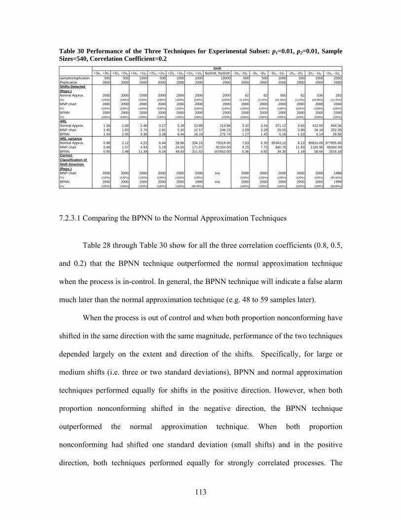
Table 30 Performance of the Three Techniques for Experimental Subset: p1=0.01, p2=0.01, Sample Sizes=540, Correlation Coefficient=0.2
Shift+3s1, +3s2 +3s1, +2s2 +3s1, +1s2 +2s1, +2s2 +2s1, +1s2 +1s1, +1s2 NoShift_NoShift -3s1, -3s2 -3s1, -2s2 -3s1, -1s2 -2s1, -2s2 -2s1, -1s2 -1s1, -1s2
samples/replication 500 500 1000 500 1000 1000 10000 500 500 1000 500 1000 2000Replication 2000 2000 2000 2000 2000 2000 2000 2000 2000 2000 2000 2000 2000Shifts Detected (Reps.)Normal Approx. 2000 2000 2000 2000 2000 2000 2000 62 62 565 62 536 283(%) (100%) (100%) (100%) (100%) (100%) (100%) (100%) (3.10%) (3.10%) (28.25%) (3.10%) (26.80%) (14.15%)MNP chart 2000 2000 2000 2000 2000 2000 2000 2000 2000 2000 2000 2000 2000(%) (100%) (100%) (100%) (100%) (100%) (100%) (100%) (100%) (100%) (100%) (100%) (100%) (100%)BPNN 2000 2000 2000 2000 2000 2000 2000 2000 2000 2000 2000 2000 2000(%) (100%) (100%) (100%) (100%) (100%) (100%) (100%) (100%) (100%) (100%) (100%) (100%) (100%)ARLNormal Approx. 1.56 2.00 2.46 3.27 5.28 13.89 213.88 3.32 3.24 371.12 3.65 412.50 844.36MNP chart 1.45 1.83 2.74 2.81 5.16 12.57 246.23 2.59 3.28 29.03 3.96 34.18 252.39BPNN 1.54 2.05 3.36 3.28 6.44 16.19 272.74 1.27 1.42 5.16 1.53 6.14 29.56ARL varianceNormal Approx. 0.88 2.12 4.23 8.44 28.96 204.15 79319.00 7.63 6.35 85343.12 8.13 90815.05 377905.66MNP chart 0.68 1.57 4.93 5.19 24.05 171.97 91334.00 4.15 7.75 840.76 11.93 1183.90 66304.30BPNN 0.90 2.48 11.38 8.24 49.43 311.52 167652.00 0.36 0.82 34.35 1.18 58.66 2016.18Correct Classification of Shift Direction (Reps.)MNP chart 2000 2000 2000 2000 2000 2000 n/a 2000 2000 2000 2000 2000 1988(%) (100%) (100%) (100%) (100%) (100%) (100%) (100%) (100%) (100%) (100%) (100%) (99.40%)BPNN 2000 2000 2000 2000 2000 1999 n/a 2000 2000 2000 2000 2000 1999(%) (100%) (100%) (100%) (100%) (100%) (99.95%) (100%) (100%) (100%) (100%) (100%) (99.95%)
7.2.3.1 Comparing the BPNN to the Normal Approximation Techniques
Table 28 through Table 30 show for all the three correlation coefficients (0.8, 0.5,
and 0.2) that the BPNN technique outperformed the normal approximation technique
when the process is in-control. In general, the BPNN technique will indicate a false alarm
much later than the normal approximation technique (e.g. 48 to 59 samples later).
When the process is out of control and when both proportion nonconforming have
shifted in the same direction with the same magnitude, performance of the two techniques
depended largely on the extent and direction of the shifts. Specifically, for large or
medium shifts (i.e. three or two standard deviations), BPNN and normal approximation
techniques performed equally for shifts in the positive direction. However, when both
proportion nonconforming shifted in the negative direction, the BPNN technique
outperformed the normal approximation technique. When both proportion
nonconforming had shifted one standard deviation (small shifts) and in the positive
direction, both techniques performed equally for strongly correlated processes. The
113

normal approximation technique outperformed the BPNN technique for moderately and
weakly correlated processes. When both proportion nonconforming had shifted one
standard deviation and in the negative direction, the BPNN technique outperformed the
normal approximation technique.
When the shifts had different magnitudes and were in the positive direction,
performance of the two techniques depended on the magnitude of the shifts. Specifically,
for a process with the proportion nonconforming of the first attribute shifted three or two
standard deviations and the proportion nonconforming of the second attribute shifted one
standard deviation, the normal approximation technique outperformed the BPNN
technique for all levels of correlation. However, when the proportion nonconforming of
the first attribute shifted three standard deviations and the proportion nonconforming of
the second attribute shifted two standard deviations, the BPNN and the normal
approximation techniques performed equally. When both proportion nonconforming
shifted with different magnitudes and in the negative direction, the BPNN technique
outperformed the normal approximation technique for all levels of correlation.
7.2.3.2 Comparing the BPNN Technique to the MNP Chart
Table 28 through Table 30 show for all the three correlation coefficients (0.8, 0.5,
and 0.2) that the BPNN technique outperformed the MNP chart when the process is in-
control. In general, the BPNN technique will indicate a false alarm much later than the
MNP chart (e.g. 5 to 26 samples later).
When the process is out of control and when both proportion nonconforming have
shifted in the same direction with the same magnitude, performance of the two techniques
114

depended largely on the extent and direction of the shifts. Specifically, for large and
medium shifts, the BPNN technique and the MNP chart performed equally for shifts in
the positive direction. When both proportion nonconforming shifted in the negative
direction with large magnitude, the BPNN technique detected shifts faster than the MNP
chart (the BPNN technique had smaller ARL than the MNP chart) for all levels of
correlation coefficient. However, for strongly and moderately correlated processes (Table
28 and Table 29) the BPNN technique could not indicate the shifts for four of the 2000
replications while the MNP chart indicated shifts for all replications. If one assumed that
the BPNN technique detected the shifts for those four replications, one might conclude
that the MNP chart performed either better than or equal to the BPNN technique.
When both proportion nonconforming shifted in the negative direction with
medium magnitude, the BPNN technique detected shifts faster than the MNP chart (the
BPNN technique had smaller ARL than the MNP chart) for all levels of correlation
coefficient. However, for strongly and moderately correlated processes the BPNN
technique could not indicate the shifts for four of the 2000 replications while the MNP
chart indicated shifts for all replications. If one assumed that the BPNN technique
detected the shifts for those four replications, one would still conclude that the BPNN
technique outperformed the MNP chart. When both proportion nonconforming had
shifted one standard deviation (small shifts) and in the positive direction, the MNP chart
outperformed the BPNN for all levels of correlation coefficients. In contrary, the BPNN
technique outperformed the MNP chart when both proportion nonconforming had shifted
in the negative direction.
115

When the shifts had different magnitudes and were in the positive direction, the
performance depended on the level of correlation coefficient and the magnitudes of the
shifts. For strongly and weakly correlated processes, the MNP chart outperformed the
BPNN technique when the proportion nonconforming of the first attribute shifted two
standard deviations and the proportion nonconforming of the second attribute shifted one
standard deviation. Both techniques performed equally for the other magnitudes of shifts.
For moderately correlated processes, both techniques performed equally. When both
proportion nonconforming shifted with different magnitudes and in the negative
direction, the BPNN technique detected shifts faster than the MNP chart (the BPNN had
smaller ARL than the MNP chart) for moderately correlated processes. However, the
BPNN technique could not indicate the shifts for four of the 2000 replications while the
MNP chart indicate shifts for all 2000 replications. If one assumed that the BPNN
technique detected the shifts for those four replications, one would conclude that the
BPNN technique outperformed the MNP chart. For weakly correlated processes, the
BPNN outperformed the MNP chart.
7.2.3.3 Comparing the MNP Chart to the Normal Approximation Technique
Table 28 through Table 30 show for all the three correlation coefficients (0.8, 0.5,
and 0.2) that the MNP chart will indicate a false alarm much later than the normal
approximation technique (e.g. 32 to 53 samples later).
When the process is out of control and when both proportion nonconforming have
shifted in the same direction with the same magnitude, performance of the two techniques
depended largely on the extent and direction of the shifts. Specifically, for large and
116

medium shifts, the MNP chart and the normal approximation technique performed
equally for shifts in the positive direction. However, when both proportion
nonconforming shifted in the negative direction, the MNP chart outperformed the normal
approximation technique. When both proportion nonconforming had shifted one standard
deviation (small shifts) and in the positive direction, the MNP chart outperformed the
normal approximation technique for all levels of correlation. When both proportion
nonconforming had shifted one standard deviation and in the negative direction, the MNP
chart outperformed the normal approximation technique.
When the shifts had different magnitudes and were in the positive direction, the
level of correlation affected the results. For strongly correlated processes, the normal
approximation technique outperformed the MNP chart when the proportion
nonconforming of the first attribute shifted three or two standard deviations and the
proportion nonconforming of the second attribute shifted one standard deviation. Both
techniques performed equally for other magnitudes of shifts. For moderately correlated
processes, the normal approximation technique outperformed the MNP chart when the
proportion nonconforming of the first attribute shifted three standard deviations and the
proportion nonconforming of the second attribute shifted one standard deviation. Both
techniques performed equally for other magnitudes of shifts. For weakly correlated
processes, the normal approximation technique and the MNP chart performed equally
when both proportion nonconforming shifted with different magnitudes. When both
proportion nonconforming shifted with different magnitudes and in the negative
direction, the MNP chart detected shifts faster than the normal approximation technique
for all levels of correlation.
117

7.3 Satisfying the Condition of Finding at Least One Nonconforming Item in a Sample
The following three sub-sections presented for varied proportion nonconforming
the pair-wise comparisons of the three techniques for the sample size that satisfies the
condition of finding at least one nonconforming item in a sample.
7.3.1 p1 = 0.3, p2 = 0.3, Sample Sizes = 10 (Levels of Correlation: 0.8, 0.5, and 0.2)
For a process with two attributes each with proportion non-conforming of 0.3, the
sample size calculated to satisfy the condition of finding at least one nonconforming item
in a sample was the same as the sample size recommended for the MNP chart. Thus, this
sub-experiment is a duplication of the sub-experiment in section 7.2.1. See results in
section 7.2.1.
7.3.2 p1 = 0.1, p2 = 0.1, Sample Sizes = 30 (Levels of Correlation: 0.8, 0.5, and 0.2)
For a process with two attributes each with proportion nonconforming of 0.1, the
sample size calculated to satisfy the condition of finding at least one nonconforming item
in a sample was the same as the sample size recommended for the MNP chart. Thus, this
sub-experiment is a duplication of the sub-experiment in section 7.2.2. See results in
section 7.2.2.
7.3.3 p1 = 0.01, p2 = 0.01, Sample Sizes = 300 (Levels of Correlation: 0.8, 0.5, and 0.2)
Table 31 through Table 36 present the ARLs for the normal approximation
technique, the MNP chart, and the BPNN technique for three of the experimental subsets
118

(proportion nonconforming p1 = 0.01 and p2 = 0.01; a sample size #3 = 300; and levels of
correlation = 0.80, 0.50, and 0.20, respectively).
The results showed that the in-control ARL for the normal approximation
technique and the MNP chart were substantially different. To compare the BPNN
technique to the normal approximation technique and the MNP chart, two different cut-
off values were used for the BPNN technique in order to have the in-control ARL
comparable to the ARL for each technique. As a result, there were two tables for an
experimental subset; the first table showed the comparison between the BPNN technique
and the normal approximation technique and the second table showed the comparison
between the BPNN technique and the MNP chart.
Table 31 Performance of the BPNN and the Normal Approximation Techniques for Experimental Subset: p1=0.01, p2=0.01, Sample Sizes=300, Correlation Coefficient=0.8
Shift+3s1, +3s2 +3s1, +2s2 +2s1, +2s2 +2s1, +1s2 +1s1, +1s2 NoShift_NoShift -3s1, -3s2 -3s1, -2s2 -2s1, -2s2 -1s1, -1s2
samples/replication 500 500 500 1000 1000 10000 500 500 500 2000Replication 10000 10000 10000 10000 10000 10000 10000 10000 10000 10000Shifts Detected (Reps.)Normal Approx. 10000 10000 10000 10000 10000 10000 9 9 9 3(%) (100%) (100%) (100%) (100%) (100%) (100%) (0.09%) (0.09%) (0.09%) (33.44%)BPNN 10000 10000 10000 10000 9999 9987 6844 6844 6844 6921(%) (100%) (100%) (100%) (100%) (99.99%) (99.87%) (68.44%) (68.44%) (68.44%) (69.21%)ARL
344
Normal Approx. 2.06 2.26 4.19 4.18 14.72 135.62 271.78 271.78 271.78 894.43BPNN 1.99 2.69 4.09 7.33 15.90 146.04 1.44 1.44 1.44 16.08ARL varianceNormal Approx. 2.29 3.14 15.56 15.20 260.42 30108.41 18016.19 18016.19 18016.19 334974.31BPNN 2.45 5.88 18.15 81.45 585.14 194096.79 0.63 0.63 0.63 14872.98
119

Table 32 Performance of the BPNN Technique and the MNP Chart for Experimental Subset: p1=0.01, p2=0.01, Sample Sizes=300, Correlation Coefficient=0.8
Shift+3s1, +3s2 +3s1, +2s2 +2s1, +2s2 +2s1, +1s2 +1s1, +1s2 NoShift_NoShift -3s1, -3s2 -3s1, -2s2 -2s1, -2s2 -1s1, -1s2
samples/replication 500 500 500 1000 1000 10000 500 500 500 2000Replication 10000 10000 10000 10000 10000 10000 10000 10000 10000 10000Shifts Detected (Reps.)MNP chart 10000 10000 10000 10000 10000 10000 10000 10000 10000 10000(%) (100%) (100%) (100%) (100%) (100%) (100%) (100%) (100%) (100%) (100%)BPNN 10000 10000 10000 10000 9999 9999 9625 9625 9625 9644(%) (100%) (100%) (100%) (100%) (99.99%) (99.99%) (96.25%) (96.25%) (96.25%) (96.44%)ARLMNP chart 1.95 2.60 3.92 6.78 14.00 30.67 1.45 1.45 1.45 4.71BPNN 1.58 2.00 2.72 4.40 7.88 34.32 1.42 1.42 1.42 6.77ARL varianceMNP chart 1.95 4.26 12.28 40.82 213.99 902.68 0.63 0.63 0.63 17.57BPNN 1.00 2.25 5.83 23.13 83.31 21711.67 0.60 0.60 0.60 3464.08Correct Classification of Shift Direction (Reps.)MNP chart 10000 9995 9979 9919 9506 n/a 10000 10000 10000 10000(%) (100%) (99.95%) (99.79%) (99.19%) (95.06%) (100%) (100%) (100%) (100%)BPNN 10000 9996 9974 9928 9661 n/a 9625 9625 9625 9618(%) (100%) (99.96%) (99.74%) (99.28%) (96.61%) (96.25%) (96.25%) (96.25%) (96.18%)
Table 33 Performance of the BPNN and the Normal Approximation Techniques for Experimental Subset: p1=0.01, p2=0.01, Sample Sizes=300, Correlation Coefficient=0.5
Shift+3s1, +3s2 +3s1, +2s2 +3s1, +1s2 +2s1, +2s2 +2s1, +1s2 +1s1, +1s2 NoShift_NoShift -3s1, -3s2 -3s1, -2s2 -2s1, -2s2 -1s1, -1s2
samples/replication 500 500 1000 500 1000 1000 10000 500 500 500 2000Replication 10000 10000 10000 10000 10000 10000 10000 10000 10000 10000 10000Shifts Detected (Reps.)Normal Approx. 10000 10000 10000 10000 10000 10000 10000 0 0 0 1108(%) (100%) (100%) (100%) (100%) (100%) (100%) (100%) (0%) (0%) (0%) (11.08%)BPNN 10000 10000 10000 10000 10000 10000 9993 8051 8051 8051 8064(%) (100%) (100%) (100%) (100%) (100%) (100%) (99.93%) (80.51%) (80.51%) (80.51%) (80.64%)ARLNormal Approx. 1.81 2.25 2.36 3.64 5.09 13.53 158.68 No detection No detection No detection 927.89BPNN 1.89 2.68 4.16 4.11 7.79 18.03 169.25 1.60 1.60 1.60 7.99ARL varianceNormal Approx. 1.58 3.11 3.43 11.26 24.01 221.55 39388.00 No detection No detection No detection 345366.26BPNN 1.81 5.35 17.23 15.59 72.99 499.85 210800.00 0.93 0.93 0.93 1762.37
120

Table 34 Performance of the BPNN Technique and the MNP Chart for Experimental Subset: p1=0.01, p2=0.01, Sample Sizes=300, Correlation Coefficient=0.5
Shift+3s1, +3s2 +3s1, +2s2 +3s1, +1s2 +2s1, +2s2 +2s1, +1s2 +1s1, +1s2 NoShift_NoShift -3s1, -3s2 -3s1, -2s2 -2s1, -2s2 -1s1, -1s2
samples/replication 500 500 1000 5000 1000 1000 10000 500 500 500 2000Replication 10000 10000 10000 10000 10000 10000 10000 10000 10000 10000 10000Shifts Detected (Reps.)MNP chart 10000 10000 10000 10000 10000 10000 10000 10000 10000 10000 10000(%) (100%) (100%) (100%) (100%) (100%) (100%) (100%) (100%) (100%) (100%) (100%)BPNN 10000 10000 10000 10000 10000 10000 10000 9719 9719 9719 9722(%) (100%) (100%) (100%) (100%) (100%) (100%) (100%) (97.19%) (97.19%) (97.19%) (97.22%)ARLMNP chart 1.71 2.29 3.34 3.38 5.95 12.86 60.05 1.61 1.61 1.61 6.73BPNN 1.65 2.15 3.13 3.12 5.42 11.23 60.96 1.57 1.57 1.57 6.56ARL varianceMNP chart 1.24 3.17 8.30 8.76 30.69 183.41 3663.40 0.94 0.94 0.94 38.75BPNN 1.10 2.72 7.74 7.72 28.88 149.29 19876.00 0.89 0.89 0.89 433.54Correct Classification of Shift Direction (Reps.)MNP chart 10000 10000 9998 9999 9988 9879 n/a 10000 10000 10000 10000(%) (100%) (100%) (99.98%) (99.99%) (99.88%) (98.79%) (100%) (100%) (100%) (100%)BPNN 10000 10000 9997 9998 9983 9884 n/a 9719 9719 9719 9717(%) (100%) (100%) (99.97%) (99.98%) (99.83%) (98.84%) (97.19%) (97.19%) (97.19%) (97.17%)
Table 35 Performance of the BPNN and the Normal Approximation Techniques for Experimental Subset: p1=0.01, p2=0.01, Sample Sizes=300, Correlation Coefficient=0.2
Shift+3s1, +3s2 +3s1, +2s2 +3s1, +1s2 +2s1, +2s2 +2s1, +1s2 +1s1, +1s2 NoShift_NoShift -3s1, -3s2 -3s1, -2s2 -3s1, -1s2 -2s1, -2s2 -2s1, -1s2 -1s1, -1s2
samples/replication 500 500 1000 5000 1000 1000 10000 500 500 1000 500 1000 2000Replication 10000 10000 10000 10000 10000 10000 10000 10000 10000 10000 10000 10000 10000Shifts Detected (Reps.)Normal Approx. 10000 10000 10000 10000 10000 10000 10000 0 0 475 0 475 629(%) (100%) (100%) (100%) (100%) (100%) (100%) (100%) (0%) (0%) (4.75%) (0%) (4.75%) (6.29%)BPNN 10000 10000 10000 10000 10000 10000 9997 9639 9639 9639 9639 9639 9639(%) (100%) (100%) (100%) (100%) (100%) (100%) (99.97%) (96.39%) (96.39%) (96.39%) (96.39%) (96.39%) (96.39%)ARLNormal Approx. 1.56 1.98 2.44 3.08 4.79 12.05 165.77 No detection No detection 490.51 No detection 490.51 1008.48BPNN 1.67 2.30 3.73 3.68 7.18 18.16 168.78 1.68 1.68 4.11 1.68 4.11 9.47ARL varianceNormal Approx. 0.95 2.14 3.99 7.01 20.41 166.86 40085.00 No detection No detection 87023.52 0.00 87023.52 326596.72BPNN 1.22 3.53 11.77 11.40 57.08 451.90 128230.00 1.20 1.20 13.14 1.20 13.14 84.19
Table 36 Performance of the BPNN Technique and the MNP Chart for Experimental Subset: p1=0.01, p2=0.01, Sample Sizes=300, Correlation Coefficient=0.2
Shift+3s1, +3s2 +3s1, +2s2 +3s1, +1s2 +2s1, +2s2 +2s1, +1s2 +1s1, +1s2 NoShift_NoShift -3s1, -3s2 -3s1, -2s2 -3s1, -1s2 -2s1, -2s2 -2s1, -1s2 -1s1, -1s2
samples/replication 500 500 1000 5000 1000 1000 10000 500 500 1000 500 1000 2000Replication 10000 10000 10000 10000 10000 10000 10000 10000 10000 10000 10000 10000 10000Shifts Detected (Reps.)MNP chart 10000 10000 10000 10000 10000 10000 10000 10000 10000 10000 10000 10000 10000(%) (100%) (100%) (100%) (100%) (100%) (100%) (100%) (100%) (100%) (100%) (100%) (100%) (100%)BPNN 10000 10000 10000 10000 10000 10000 9999 9923 9923 9923 9923 9923 9923(%) (100%) (100%) (100%) (100%) (100%) (100%) (99.99%) (99.23%) (99.23%) (99.23%) (99.23%) (99.23%) (99.23%)ARLMNP chart 1.46 1.87 2.79 2.79 4.92 11.40 103.67 1.72 1.72 4.25 1.72 4.25 9.96BPNN 1.52 1.99 3.09 3.05 5.56 13.00 108.93 1.62 1.62 3.81 1.62 3.81 8.57ARL varianceMNP chart 0.71 1.77 5.23 5.13 21.34 141.29 12108.00 1.26 1.26 13.59 1.26 13.59 88.62BPNN 0.87 2.22 7.60 7.35 30.71 211.04 29860.00 1.07 1.07 12.31 1.07 12.31 74.91Correct Classification of Shift Direction (Reps.)MNP chart 10000 10000 10000 10000 9994 9982 n/a 10000 10000 10000 10000 10000 10000(%) (100%) (100%) (100%) (100%) (99.94%) (99.82%) (100%) (100%) (100%) (100%) (100%) (100%)BPNN 10000 9999 9999 10000 9993 9961 n/a 9923 9923 9923 9923 9923 9923(%) (100%) (99.99%) (99.99%) (100%) (99.93%) (99.61%) (99.23%) (99.23%) (99.23%) (99.23%) (99.23%) (99.23%)
121

7.3.3.1 Comparing BPNN to the Normal Approximation Techniques
Table 31, Table 33, and Table 35 show for all the three correlation coefficients
(0.8, 0.5, and 0.2) that BPNN technique outperformed the normal approximation
technique when the process is in-control. In general, the BPNN technique will indicate a
false alarm much later than the normal approximation technique (e.g. 3 to 11 samples
later).
When the process is out of control and when both proportion nonconforming have
shifted in the same direction with the same magnitude, performance of the two techniques
depended largely on the extent and direction of the shifts. Specifically, for large or
medium shifts (i.e. three or two standard deviations), BPNN and normal approximation
techniques performed equally for shifts in the positive direction. However, when both
proportion nonconforming shifted in the negative direction, the BPNN technique
outperformed the normal approximation technique (the normal approximation technique
could not detect any shift). When both proportion nonconforming had shifted one
standard deviation (small shifts) and in the positive direction, the normal approximation
outperformed the BPNN technique for all levels of correlation coefficient. When both
proportion nonconforming had shifted one standard deviation and in the negative
direction, the BPNN technique outperformed the normal approximation technique.
When the shifts had different magnitudes and they were in the positive direction,
performance of the two techniques depended on the magnitude of shifts. Specifically, for
a process with the proportion nonconforming of the first attribute shifted three or two
standard deviations and the proportion nonconforming of the second attribute shifted one
standard deviation, the normal approximation technique outperformed the BPNN
122

technique for all levels of correlation. However, when the proportion nonconforming of
the first attribute shifted three standard deviations and the proportion nonconforming of
the second attribute shifted two standard deviations, the BPNN and the normal
approximation technique performed equally. When both proportion nonconforming
shifted with different magnitudes and in the negative direction, the BPNN technique
outperformed the normal approximation technique for all levels of correlation.
7.3.3.2 Comparing BPNN to the MNP Chart
Table 32, Table 34, and Table 36 show for all the three correlation coefficients
(0.8, 0.5, and 0.2) that the BPNN technique outperformed the MNP chart when the
process is in-control. In general, the BPNN technique will indicate a false alarm much
later than the MNP chart (e.g. 4 to 5 samples later).
When the process is out of control and when both proportion nonconforming have
shifted in the same direction with the same magnitude, performance of the two techniques
depended largely on the extent and direction of the shifts. Specifically, for large shifts,
the BPNN technique and the MNP chart performed equally for shifts in the positive
direction. When both proportion nonconforming shifted in the negative direction, both
techniques had the same ARL for all levels of correlation coefficients. However, the
BPNN technique could not indicate the shifts for all of the replications while the MNP
chart could. If one assumed that the BPNN technique detected the shifts for those
replications, one would conclude that the MNP chart outperformed the BPNN technique.
For processes with medium shifts and both proportion nonconforming shifted in the
positive direction, the BPNN technique detected shifts faster than the MNP chart (the
123

BPNN had smaller ARL than the MNP chart) for strongly correlated processes. However,
the MNP chart identified the direction of shifts more correctly than the BPNN technique.
This difference was considered insignificant. For processes with medium shifts and both
proportion nonconforming shifted in the positive direction, the BPNN had the same ARL
as the MNP chart for moderately and weakly correlated processes. However, the MNP
chart identified the direction of shifts more correctly than the BPNN technique for
moderately correlated processes. Again, this difference was considered insignificant.
When both proportion nonconforming shifted in the negative direction, both techniques
had the same ARL for all levels of correlation coefficients. However, the BPNN
technique could not indicate the shifts for all of the replications while the MNP chart
could. If one assumed that the BPNN technique detected the shifts for those replications,
one would conclude that the MNP chart outperformed the BPNN technique. When both
proportion nonconforming had shifted one standard deviation (small shifts) and in the
positive direction, the BPNN technique outperformed the MNP chart for all strongly and
moderately correlated processes. In contrary, the MNP chart outperformed the BPNN for
weakly correlated processes. When both proportion nonconforming had shifted in the
negative direction, the MNP chart outperformed the BPNN for strongly correlated
processes. For moderately and weakly correlated processes, the BPNN technique had
ARL equal to and smaller than the MNP chart respectively. However, the BPNN
technique could not indicate the shifts for all of the replications while the MNP chart
could. If one assumed that the BPNN technique detected the shifts for those replications,
one would conclude that the MNP chart outperformed the BPNN technique.
124

When the shifts had different magnitudes and were shifted in the positive
direction, the performance depended on the level of correlation coefficient and the
magnitude of the shifts. For strongly correlated processes, the BPNN technique
outperformed the MNP chart when the proportion nonconforming of the first attribute
shifted two standard deviations and the proportion nonconforming of the second attribute
shifted one standard deviation. Both techniques performed equally for other magnitudes
of shifts. For moderately correlated processes, both techniques had the same ARL for all
magnitudes of shifts. However, the MNP chart identified the direction of shifts more
correctly than the BPNN technique when the proportion nonconforming of the first
attribute shifted three or two standard deviations and the proportion nonconforming of the
second attribute shifted one standard deviation. These differences were considered
insignificant. For weakly correlated processes, both techniques had equal ARL but the
MNP chart could identify the direction of shifts more correctly than the BPNN technique.
Again, these differences were considered insignificant.
When both proportion nonconforming shifted with different magnitudes and in
the negative direction, the MNP chart outperformed the BPNN technique. Both
techniques had equal ARL but the BPNN technique could not indicate the shifts for all of
the replications while the MNP chart could. If one assumed that the BPNN technique
detected the shifts for those replications, one would conclude that the MNP chart
outperformed the BPNN technique.
125

7.3.3.3 Comparing the MNP Chart to the Normal Approximation Technique
Table 31 through Table 36 show for all the three correlation coefficients (0.8, 0.5,
and 0.2) that the normal approximation technique outperformed the MNP chart when the
process is in-control. In general, the normal approximation technique will indicate a false
alarm much later than the MNP chart (e.g. 62 to 105 samples later).
When the process is out of control and when both proportion nonconforming have
shifted in the same direction with the same magnitude, performance of the two techniques
depended largely on the direction of the shifts. Specifically, for large, medium, and small
shifts, the MNP chart and the normal approximation technique performed equally when
both proportion nonconforming shifted in the positive direction. However, when both
proportion nonconforming shifted in the negative direction, the MNP chart outperformed
the normal approximation technique.
When the shifts had different magnitudes and were in the positive direction, the
level of correlation affected the results. For strongly correlated processes, the normal
approximation technique outperformed the MNP chart when the proportion
nonconforming of the first attribute shifted two standard deviations and the proportion
nonconforming of the second attribute shifted one standard deviation. Both techniques
performed equally for other magnitudes of shift. For moderately correlated processes, the
normal approximation technique outperformed the MNP chart when the proportion
nonconforming of the first attribute shifted three standard deviations and the proportion
nonconforming of the second attribute shifted one standard deviation. Both techniques
performed equally for other magnitudes of shift. For weakly correlated processes, the
normal approximation technique and the MNP chart performed equally when both
126

proportion nonconforming shifted with any magnitude. When both proportion
nonconforming shifted with different magnitudes and in the negative direction, the MNP
chart detected shifts faster than the normal approximation technique for all levels of
correlation.
127

8.0 RECCOMENDATION FOR IMPLEMENTATION
This chapter provides summary of the results and how they may be implemented
for practical use. Section 8.1 discusses guidelines for selecting a suitable technique for a
particular process condition. General performances for the three multi-attribute process
control techniques are summarized in section 8.2. Finally, the interpretation of out-of-
control signals is discussed in section 8.3.
The results for large sample sizes (sample size #1: estimating multivariate
normally distributed variables from a multivariate binomial distribution) discussed in
section 7.1 are summarized in Table 37 through Table 39.
Table 37 Comparisons of the BPNN and Normal Approximation Techniques for Large Sample Sizes.
Status of Process's Proportion Nonconforming Sample Size # 1p1=0.3,p2=0.3,n=50 p1=0.1,p2=0.1,n=100 p1=0.01,p2=0.01,n=910
In-control B>N B>N B>NOut-of-control with the same magnitude of shiftslarge shift in the positive direction B=N B=N B=Nlarge shift in the negative direction B>N(S.C.), B=N (M.C.&W.C.) B>N (S.C.&M.C.), B=N (W.C.) B>Nmedium shift in the positive direction B>N B=N B=Nmedium shift in the negative direction B>N B>N B>Nsmall shift in the positive direction B>N B>N B>Nsmall shift in the negative direction B>N B>N B>NOut-of-control with different magnitude of shifts Strong Mod. Weak Strong Mod. Weak Strong Mod. Weak3s,2s B=N B=N B=N B=N B=N B=N B=N B=N B=N3s,1s n/a N>B B=N n/a N>B B=N N>B N>B B=N2s,1s N>B B=N B>N N>B B=N B=N N>B B=N B=N-3s,-2s n/a B>N B=N n/a n/a B>N n/a n/a n/a-3s,-1s n/a N>B B=N n/a n/a B>N n/a n/a n/a-2s,-1s N>B B>N B>N n/a B>N B>N n/a B>N B>N
128

Table 38 Comparisons of the BPNN Technique and the MNP chart for Large Sample Sizes. Status of Process's Proportion Nonconforming Sample Size # 1
p1=0.3,p2=0.3,n=50 p1=0.1,p2=0.1,n=100 p1=0.01,p2=0.01,n=910In-control B>M B>M B>MOut-of-control with the same magnitude of shiftslarge shift in the positive direction B=M B=M B=Mlarge shift in the negative direction B=M B=M (S.C.#&M.C.# &W.C.) M>B(S.C.)@, M=or>B(M.C.)+, B=M (W.C.)medium shift in the positive direction B=M B=M B=Mmedium shift in the negative direction B=M B>M(S.C.)*,M>B(M.C.),B=M(W.C.) B>M (S.C.)*,M=or>B (M.C.)+, M>B(W.C.)small shift in the positive direction M>B(S.C&M.C.&W.C*) M>B(S.C.&M.C.), B=M(W.C.) B=M (S.C.#&M.C.&W.C.)small shift in the negative direction B>M(S.C.),M>B(M.C.&W.C.)* B>M(S.C.)*,M>B(M.C.&W.C.) B>M(S.C.&M.C.*),M>B(W.C.)Out-of-control with different magnitude of shifts Strong Mod. Weak Strong Mod. Weak Strong Mod. Weak3s,2s B=M B=M B=M B=M B=M B=M B=M B=M B=M3s,1s n/a B=M B=M n/a B=M B=M B=M B=M B=M2s,1s B=M B=M B=M B=M B=M B=M B=M B=M B=M-3s,-2s n/a B=M B=M n/a n/a B=M n/a n/a n/a-3s,-1s n/a B=M B=M n/a n/a M>B n/a n/a n/a-2s,-1s B=M# B=M# M>B n/a M>B M>B n/a M>B M>B
Table 39 Comparisons of the MNP Chart and the Normal Approximation Technique for Large Sample Sizes. Status of Process's Proportion Nonconforming Sample Size # 1
p1=0.3,p2=0.3,n=50 p1=0.1,p2=0.1,n=100 p1=0.01,p2=0.01,n=910In-control M>N(S.C.),N>M(M.C.&W.C.) M>N M>NOut-of-control with the same magnitude of shiftslarge shift in the positive direction M=N M=N M=Nlarge shift in the negative direction M>N(S.C.), M=N (M.C.&W.C.) M>N (S.C.&M.C.), M=N (W.C.) M>Nmedium shift in the positive direction M>N M=N M=Nmedium shift in the negative direction M>N M>N M>N small shift in the positive direction M>N M>N M>Nsmall shift in the negative direction M>N M>N M>NOut-of-control with different magnitude of shifts Strong Mod. Weak Strong Mod. Weak Strong Mod. Weak3s,2s M=N M=N M=N M=N M=N M=N M=N M=N M=N3s,1s n/a N>M M=N n/a N>M M=N N>M N>M M=N2s,1s N>M M=N M>N N>M M=N M=N N>M M=N M=N-3s,-2s n/a M>N M=N n/a n/a M>N n/a n/a n/a-3s,-1s n/a N>M M=N n/a n/a M>N n/a n/a n/a-2s,-1s N>M M>N M>N n/a M>N M>N n/a M>N M>N
Remark: S.C., M.C., and W.C. are strong, moderate, and weak correlation coefficients.
The symbol (>) shown in the tables indicates which technique “outperforms” the
other technique (e.g. B>N represents the BPNN technique is better than the normal
approximation technique). Some of the techniques outperform the other two for certain
specified process conditions while they are inferior in other process conditions. To select
a suitable technique, users must weigh the in-control against the out-of-control average
run length. If stopping a process to investigate the out-of-control signal is critical, a
technique with a large in-control ARL is recommended. For instance, the BPNN
technique is preferred for a strongly correlated process with large proportion
129

nonconforming when both proportion nonconforming only shift with the same magnitude
and in the same direction (either positive or negative). In this condition, the BPNN
technique detects a false alarm 61 and 20 samples later than the normal approximation
technique and the MNP chart respectively, as shown in Table 6. In addition, the BPNN
technique has an out-of-control ARL either smaller than or equal to the normal
approximation technique. The out-of-control ARL for the BPNN and the MNP chart are
equal when both proportion nonconforming shift from medium to large magnitude. The
MNP chart detects shifts faster than the BPNN by only one ARL sample when both
proportion nonconforming shift with a small magnitude and in the positive direction. The
BPNN detects shifts faster than the MNP chart four ARL samples when both proportion
nonconforming shift with a small magnitude and in the negative direction.
In contrary, if a process needs to be adjusted quickly from an out-of-control status
to an in-control status, one might select a technique with a small out-of-control ARL for
quick detection. For example, the MNP chart is preferred for a process with two weakly
correlated attributes each having proportion nonconforming of 0.01. Both of the process’s
proportion nonconforming often shift with the same magnitude in the same direction,
either positive or negative, and the sample sizes are large. The BPNN technique indicates
a false alarm 22 and 53 samples later than the MNP chart and the normal approximation
technique respectively as shown in Table 14. The MNP chart designates a false alarm 31
samples later than the normal approximation technique. All techniques performed equally
when both proportion nonconforming shift from medium to large magnitudes and in the
positive direction. The MNP chart and the BPNN technique outperform the normal
approximation when both proportion nonconforming shift in the negative direction. The
130

MNP chart outperforms the BPNN when both proportion nonconforming shift with
medium and small magnitudes in the negative directions.
In comparing the BPNN technique and the MNP chart, the two techniques did not
always detect the shifts for all of the replications. As a result, it is unclear how to evaluate
the performances of both techniques since the ARL results contradict the number of
replications detected by each technique. For example, the BPNN technique had a smaller
ARL than the MNP chart; however, the MNP chart detected the shifts for all of the
replications while the BPNN technique failed to detect the shift for one replication.
Furthermore, the ARL results contradict the number of correct classifications, i.e. the
BPNN technique had a smaller out-of-control ARL than the MNP chart but the MNP
chart correctly classified the direction of shifts more than the BPNN. The difference of
the number of replications detected and the correct classification may or may not be
significant to the ARL results.
Though not the majority, such contradictory results require decision rules to guide
the user in determining which technique (BPNN or MNP) is best to apply. Table 40
provides the decision (i.e. yes or no) of whether or not there is a significant difference
between the number of replications detected and the correct classification in comparison
to the ARL results. The different situations are denoted by the superscripts, which are
also shown in Table 38, Table 43, and Table 46.
131

Table 40 Meaning of Superscripts Used in the Comparisons between the BPNN technique and the MNP Chart.
SuperscriptComparison
Results
Out-of-Control ARL X
compare to Out-of-Control ARL Y
Number of Replications Detected
Correct Classification of Shift Direction
Significance of the Difference of the Number of Replications Detected and
the Correct Classification of Shift Direction
* X>Y ARLX smaller than ARLY Rep.X equal Rep.Y Y more correct than X no* X>Y ARLX smaller than ARLY Rep.X more than Rep.Y Y more correct than X no* X>Y ARLX smaller than ARLY Rep.X less than Rep.Y Y more correct than X no# X=Y ARLX equal ARLY Rep.X equal Rep.Y X more correct than Y no# X=Y ARLX equal ARLY Rep.X less than Rep.Y Y more correct than X no# X=Y ARLX equal ARLY Rep.X equal Rep.Y Y more correct than X no@ X>Y ARLX equal ARLY Rep.X more than Rep.Y X more correct than Y yes@ X>Y ARLX larger than ARLY Rep.X more than Rep.Y X more correct than Y yes+ X= or >Y ARLX larger than ARLY Rep.X more than Rep.Y X more correct than Y yes+ X= or >Y ARLX equal ARLY Rep.X more than Rep.Y X more correct than Y yes
X and Y in Table 40 can be either BPNN technique or MNP chart. Rep.X and Rep.Y
represent the number of replications that X and Y techniques detect shifts respectively.
None of the three techniques had equal in-control ARL for a number of reasons.*
Although attempts were made to initialize the three techniques to have the same ARL, the
initial process conditions (i.e. sample size, proportion nonconforming, level of
correlation, etc.) often made this impossible. However, if one assumes equal in-control
ARL, comparisons of the three techniques are shown in Table 41, which is a summary of
Table 37 through Table 39.
* In some cases differences in the in-control ARL differed as much as 90 samples or as small as eight samples depending on the techniques compared and the process conditions.
132

Table 41 The BPNN, MNP Chart and the Normal Approximation Technique for Large Sample Sizes. (Best performing techniques in each situation are shown by their first letters) Status of Process's Proportion Nonconforming Sample Size # 1
p1=0.3,p2=0.3,n=50 p1=0.1,p2=0.1,n=100 p1=0.01,p2=0.01,n=910In-control B,M,
N N N
N N NN( N(W
N N
N N N N N N N N NN N N N N N N
N N N N N N N NN
N NN
B,M, B,M,Out-of-control with the same magnitude of shiftslarge shift in the positive direction B,M, B,M, B,M,large shift in the negative direction B,M(S.C.), B,M, M.C.&W.C.) B,M(S.C.&M.C.), B,M, .C.) M(S.C&M.C..),B,M,(W.C.)medium shift in the positive direction B,M B,M, B,M,medium shift in the negative direction B,M B(S.C.),M(M.C.),B,M(W.C.) B(S.C.), M(M.C.&W.C.)small shift in the positive direction M M(S.C.&M.C.),B,M(W.C.) B,Msmall shift in the negative direction B(S.C.),M(M.C.&W.C.) B(S.C.),M(M.C.&W.C.) B(S.C.&M.C.),M(W.C.)Out-of-control with different magnitude of shifts Strong Mod. Weak Strong Mod. Weak Strong Mod. Weak3s,2s B,M, B,M, B,M, B,M, B,M, B,M, B,M, B,M, B,M,3s,1s n/a B,M, n/a B,M, B,M,2s,1s B,M, B,M B,M, B,M, B,M, B,M,-3s,-2s n/a B,M B,M, n/a n/a B,M n/a n/a n/a-3s,-1s n/a B,M, n/a n/a M n/a n/a n/a-2s,-1s B,M M n/a M M n/a M M
Table 41 presents the comparisons among the normal approximation technique,
the MNP chart, and the BPNN technique for varied process conditions and when the
sample sizes are large. One can use the table as a guideline to select the technique that
most suitable to a particular process condition. For instance, the BPNN technique and the
MNP chart are preferred for a process with two strongly correlated attributes, each having
a large proportion nonconforming. The sample size is large and the proportion
nonconforming are expected to shift from medium to large magnitude in either positive
or negative direction.
The results also show that for any value of proportion nonconforming and level of
correlation, all techniques performed equally when both of the process’s proportion
nonconforming shift with large magnitudes and in the positive direction.
The table further indicates that the MNP chart is preferred for a weakly correlated
process for which both proportion nonconforming shift with the same magnitude. This
applies to any level of proportion nonconforming.
It can be noticed that the normal approximation technique is preferred when both
proportion nonconforming shift only in the positive direction and with different
magnitudes. This is correct for strongly and moderately correlated processes for any level
133

of in-control proportion nonconforming. For example, the normal approximation
outperformed the other methods for moderately correlated processes when the proportion
nonconforming of the first attribute shifts three standard deviations and the proportion
nonconforming of the second attribute shifts one standard deviation. All three methods
performed equally for the other magnitudes of shift. As a result, the normal
approximation technique is recommended.
The results discussed in section 7.2 for sample sizes recommended for the MNP
chart (sample size #2) are summarized in Table 42 through Table 44.
Table 42 Comparisons of the BPNN and Normal Approximation Techniques for the MNP Chart Sample Sizes. Status of Process's Proportion Nonconforming Sample Size # 2
p1=0.3,p2=0.3,n=10 p1=0.1,p2=0.1,n=30 p1=0.01,p2=0.01,n=810,670,540In-control B>N B>N B>NOut-of-control with the same magnitude of shiftslarge shift in the positive direction B=N B=N B=Nlarge shift in the negative direction B>N B>N B>Nmedium shift in the positive direction B>N(S.C.), B=N (M.C), N>B(W.C.) B=N B=Nmedium shift in the negative direction B>N B>N B>Nsmall shift in the positive direction B>N(S.C.), N>B (M.C.&W.C.) B=N(S.C.), N>B (M.C.&W.C.) B=N(S.C.), N>B (M.C.&W.C.)small shift in the negative direction B>N B>N B>NOut-of-control with different magnitude of shifts Strong Mod. Weak Strong Mod. Weak Strong Mod. Weak3s,2s n/a B=N B=N B=N B=N B=N B=N B=N B=N3s,1s n/a N>B N>B n/a N>B N>B N>B N>B N>B2s,1s n/a N>B N>B N>B N>B N>B N>B N>B N>B-3s,-2s B>N B>N B>N B>N B>N B>N n/a B>N B>N-3s,-1s n/a n/a B>N n/a n/a n/a n/a n/a B>N-2s,-1s n/a n/a B>N n/a n/a n/a n/a B>N B>N
Table 43 Comparisons of the BPNN Technique and the MNP chart for the MNP Chart Sample Sizes.
Status of Process's Proportion Nonconforming Sample Size # 2p1=0.3,p2=0.3,n=10 p1=0.1,p2=0.1,n=30 p1=0.01,p2=0.01,n=810,670,540
In-control B>M B>M B>MOut-of-control with the same magnitude of shiftslarge shift in the positive direction B=M B=M B=Mlarge shift in the negative direction M>B@ M>B@ M=or>B(S.C.&M.C.)+, B>M (W.C.)medium shift in the positive direction B>M(S.C.), B=M (M.C&W.C.) B=M (S.C.#&M.C&W.C.) B=Mmedium shift in the negative direction M>B@ M>B@ B>M(S.C.*&M.C.*&W.C.)small shift in the positive direction B>M (S.C.),B=M (M.C.)#,M>B (W.C.) B>M (S.C.&M.C.*),B=M (W.C.)# M>Bsmall shift in the negative direction M>B@ M>B (S.C.&M.C.@&W.C.@) B>MOut-of-control with different magnitude of shifts Strong Mod. Weak Strong Mod. Weak Strong Mod. Weak3s,2s n/a B=M B=M B=M B=M B=M B=M B=M B=M3s,1s n/a B=M B=M n/a B=M B=M B=M B=M B=M2s,1s n/a B=M M>B B>M B=M# B=M M>B B=M M>B-3s,-2s M>B@ M>B@ M>B@ M>B@ M>B@ M>B@ n/a B>M* B>M-3s,-1s n/a n/a M>B@ n/a n/a n/a n/a n/a B>M-2s,-1s n/a n/a M>B@ n/a n/a n/a n/a B>M* B>M
134

Table 44 Comparisons of the MNP chart and the Normal Approximation Technique for the MNP Chart Sample Sizes. Status of Process's Proportion Nonconforming Sample Size # 2
p1=0.3,p2=0.3,n=10 p1=0.1,p2=0.1,n=30 p1=0.01,p2=0.01,n=810,670,540In-control N>M N>M M>NOut-of-control with the same magnitude of shiftslarge shift in the positive direction M=N M=N M=Nlarge shift in the negative direction M>N M>N M>Nmedium shift in the positive direction M>N M=N M=Nmedium shift in the negative direction M>N M>N M>Nsmall shift in the positive direction M>N M>N M>Nsmall shift in the negative direction M>N M>N M>NOut-of-control with different magnitude of shifts Strong Mod. Weak Strong Mod. Weak Strong Mod. Weak3s,2s n/a M=N M=N M=N M=N M=N M=N M=N M=N3s,1s n/a N>M M=N n/a N>M M=N N>M N>M M=N2s,1s n/a M=N M>N N>M M=N M=N N>M M=N M=N-3s,-2s M>N M>N M>N M>N M>N M>N n/a M>N M>N-3s,-1s n/a n/a M>N n/a n/a n/a n/a n/a M>N-2s,-1s n/a n/a M>N n/a n/a n/a n/a M>N M>N
The in-control ARL for the normal approximation technique and the MNP chart
were substantially different, as mentioned in section 7.2. In order to compare the BPNN
technique to the normal approximation technique and the MNP chart, two different cut-
off values were used to obtain comparable in-control ARL. As a result, the BPNN in
Table 42 and Table 43 have different in-control ARL and the three tables cannot be
combined into a summary table.
For the sample sizes recommended for the MNP chart, Table 42 shows that the
BPNN technique outperformed the normal approximation technique when shifts were in
the negative direction for any level of proportion nonconforming and level of correlation
coefficient. The normal approximation technique cannot detect shifts that are close to “0”
and in the negative direction.
The normal approximation technique performed better than the BPNN technique
when both proportion nonconforming shifted in the positive direction and with different
magnitudes, i.e. the proportion nonconforming of the first attribute shifted with either
three or two standard deviations and the proportion nonconforming of the second
135

attribute shifted with one standard deviation. This applies to processes with all levels of
proportion nonconforming and correlation coefficient.
Table 44 shows that the normal approximation technique indicates a false alarm
later than the MNP chart when proportion nonconforming is either large or medium (0.3
or 0.1) for the sample sizes suggested by the MNP chart (sample size #2). This result is
due to the fact that the in-control ARL for the MNP chart drops significantly when the
sample sizes suggested for the MNP chart (sample size #2) are used instead of the large
sample sizes (sample size #1). For instance, a process with two strongly correlated
attributes each having proportion nonconforming of 0.3 will indicate a false alarm every
411 samples when the large sample size is used as shown in Table 6. Whereas the process
will designate a false alarm every 58 samples when smaller sample sizes (as
recommended by the MNP chart) are used as shown in Table 17. However, the MNP
chart will indicate a false alarm later than the normal approximation technique for
processes with small proportion nonconforming (0.01).
The MNP chart outperforms the normal approximation technique for all levels of
proportion nonconforming and correlation coefficient when both proportion
nonconforming shift with any magnitude in the negative direction. Also, the MNP chart
performs better than the normal approximation technique for all levels of proportion
nonconforming and level of correlation coefficient when both proportion nonconforming
shift with the same magnitude in either the positive or the negative direction.
For a strongly correlated process with any level of proportion nonconforming, the
normal approximation technique outperforms the MNP chart when the proportion
nonconforming of the first attribute shifts with either three or two standard deviations and
136

the proportion nonconforming of the second attribute shifts one standard deviation and
both proportion nonconforming shift in the positive direction. For a moderately correlated
process with any level of proportion nonconforming, the normal approximation technique
outperforms the MNP chart when the proportion nonconforming of the first attribute
shifts three standard deviations and the proportion nonconforming of the second attribute
shifts one standard deviation and both proportion nonconforming shift in the positive
direction.
When selecting between the MNP chart and the normal approximation technique
one must weigh the criticality between stopping the process to investigate the out-of-
control signal and adjusting the out-of-control process to get it back into in-control status
as fast as possible. For example, if one is concerned about identifying the out-of-control
signal as fast as possible, the MNP chart is preferred for a process with two strongly
correlated attributes each having a large proportion nonconforming.
For this process condition, the in-control ARL for the MNP chart is
approximately one-fourth the size (58 for the MNP chart as shown in Table 17 and 249
for the normal approximation technique as shown Table 16) of the normal approximation
technique. Therefore, if a process requires substantial resources to stop and investigate
potential out-of-control causes, the normal approximation is preferred. However, the
normal approximation technique cannot detect shifts that are close to “0” and in the
negative direction. For this particular situation, the BPNN technique is preferred to the
normal approximation technique since the BPNN indicates a false alarm 38 samples later
than the normal approximation technique (287 for the BPNN and 249 for the normal
approximation technique as shown in Table 16). Furthermore, the BPNN technique
137

detects shifts faster than the normal approximation technique when processes are out-of-
control (proportion nonconforming shift with any magnitude and direction).
The results discussed in section 7.3 for sample sizes that satisfy the condition of
finding at least one nonconforming item in a sample (sample size #3) are summarized in
Table 45 through Table 47. Note, the first two columns of each table are the same as for
Table 42 through Table 44 because the sample sizes were the same.
Table 45 Comparisons of the BPNN and Normal Approximation Techniques for the Small Sample Sizes.
Status of Process's Proportion Nonconforming Sample Size # 3p1=0.3,p2=0.3,n=10 p1=0.1,p2=0.1,n=30 p1=0.01,p2=0.01,n=300
In-control B>N B>N B>NOut-of-control with the same magnitude of shiftslarge shift in the positive direction B=N B=N B=Nlarge shift in the negative direction B>N B>N B>Nmedium shift in the positive direction B>N(S.C.), B=N (M.C), N>B(W.C.) B=N B=Nmedium shift in the negative direction B>N B>N B>Nsmall shift in the positive direction B>N(S.C.), N>B (M.C.&W.C.) B=N(S.C.), N>B (M.C.&W.C.) N>Bsmall shift in the negative direction B>N B>N B>NOut-of-control with different magnitude of shifts Strong Mod. Weak Strong Mod. Weak Strong Mod. Weak3s,2s n/a B=N B=N B=N B=N B=N B=N B=N B=N3s,1s n/a N>B N>B n/a N>B N>B n/a N>B N>B2s,1s n/a N>B N>B N>B N>B N>B N>B N>B N>B-3s,-2s B>N B>N B>N B>N B>N B>N B>N B>N B>N-3s,-1s n/a n/a B>N n/a n/a n/a n/a n/a B>N-2s,-1s n/a n/a B>N n/a n/a n/a n/a n/a B>N
Table 46 Comparisons of the BPNN Technique and the MNP chart for the Small Sample Sizes.
Status of Process's Proportion Nonconforming Sample Size # 3p1=0.3,p2=0.3,n=10 p1=0.1,p2=0.1,n=30 p1=0.01,p2=0.01,n=300
In-control B>M B>M B>MOut-of-control with the same magnitude of shiftslarge shift in the positive direction B=M B=M B=Mlarge shift in the negative direction M>B@ M>B@ M>B@
medium shift in the positive direction B>M(S.C.), B=M (M.C&W.C.) B=M (S.C.#&M.C&W.C.) B>M(S.C.)*, B=M (M.C.#&W.C.)medium shift in the negative direction M>B@ M>B@ M>B@
small shift in the positive direction B>M (S.C.),B=M (M.C.)#,M>B (W.C.) B>M (S.C.&M.C.*),B=M (W.C.)# B>M (S.C.&M.C.),M>B (W.C.)small shift in the negative direction M>B@ M>B (S.C.&M.C.@&W.C.@) M>B (S.C.&M.C.@&W.C.@)Out-of-control with different magnitude of shifts Strong Mod. Weak Strong Mod. Weak Strong Mod. Weak3s,2s n/a B=M B=M B=M B=M B=M B=M# B=M B=M#
3s,1s n/a B=M B=M n/a B=M B=M n/a B=M# B=M#
2s,1s n/a B=M M>B B>M B=M# B=M B>M B=M# B=M#
-3s,-2s M>B@ M>B@ M>B@ M>B@ M>B@ M>B@ M>B@ M>B@ M>B@
-3s,-1s n/a n/a M>B@ n/a n/a n/a n/a n/a M>B@
-2s,-1s n/a n/a M>B@ n/a n/a n/a n/a n/a M>B@
138

Table 47 Comparisons of the MNP chart and the Normal Approximation Technique for the Small Sample Sizes. Status of Process's Proportion Nonconforming Sample Size # 3
p1=0.3,p2=0.3,n=10 p1=0.1,p2=0.1,n=30 p1=0.01,p2=0.01,n=300In-control N>M N>M N>MOut-of-control with the same magnitude of shiftslarge shift in the positive direction M=N M=N M=Nlarge shift in the negative direction M>N M>N M>Nmedium shift in the positive direction M>N M=N M=Nmedium shift in the negative direction M>N M>N M>Nsmall shift in the positive direction M>N M>N M=Nsmall shift in the negative direction M>N M>N M>NOut-of-control with different magnitude of shifts Strong Mod. Weak Strong Mod. Weak Strong Mod. Weak3s,2s n/a M=N M=N M=N M=N M=N M=N M=N M=N3s,1s n/a N>M M=N n/a N>M M=N n/a N>M M=N2s,1s n/a M=N M>N N>M M=N M=N N>M M=N M=N-3s,-2s M>N M>N M>N M>N M>N M>N M>N M>N M>N-3s,-1s n/a n/a M>N n/a n/a n/a n/a n/a M>N-2s,-1s n/a n/a M>N n/a n/a n/a n/a n/a M>N
As mentioned in section 7.3 the in-control ARL for the normal approximation
technique and the MNP chart were substantially different. To compare the BPNN
technique to the normal approximation technique and the MNP chart, two different cut-
off values were used for the BPNN technique in order to have comparable in-control
ARL for each technique. As a result, the three tables cannot be combined into a summary
table.
For small sample sizes, Table 45 shows that the BPNN outperformed the normal
approximation technique when shifts were in the negative direction for any level of
proportion nonconforming and level of correlation coefficient. The normal approximation
technique cannot detect shifts that are close to “0” and in the negative direction.
The normal approximation technique performed better than the BPNN technique
when both of the process’s proportion nonconforming shifted in the positive direction and
with different magnitudes, i.e. the proportion nonconforming of the first attribute shifted
with either three or two standard deviations and the proportion nonconforming of the
second attribute shifted with one standard deviation. This result applies to all levels of
proportion nonconforming and correlation coefficient.
139

Table 46 indicates that the BPNN technique designates a false alarm later than the
MNP chart. However, the MNP chart detects shifts faster than the BPNN technique for
all levels of proportion nonconforming and correlation coefficient when both proportion
nonconforming shift in negative direction.
Table 47 shows that the normal approximation technique indicates a false alarm
later than the MNP chart when the proportion nonconforming varied from large to small
for small sample sizes (sample size #3). This is due to the fact that the in-control ARL for
the MNP drops significantly when small sample sizes (sample size #3) are used instead of
sample sizes prescribed by the normal approximation (sample size #1).
The MNP chart outperforms the normal approximation technique for all levels of
proportion nonconforming and correlation when both proportion nonconforming shift
with any magnitude in the negative direction. Also, the MNP chart performs better than
the normal approximation technique for all levels of proportion nonconforming and
correlation coefficient when both proportion nonconforming shift with the same
magnitude in either the positive or the negative direction.
For a strongly correlated process at any levels of proportion nonconforming, the
normal approximation technique outperforms the MNP chart when the proportion
nonconforming for the first attribute shifts two standard deviations and the proportion
nonconforming for the second attribute shifts one standard deviation and both shifts are
in the positive direction. For a moderately correlated process at any levels of proportion
nonconforming, the normal approximation technique outperforms the MNP chart when
the proportion nonconforming for the first attribute shifts three standard deviations and
140

the proportion nonconforming for the second attribute shifts one standard deviation and
both shifts are in the positive direction.
8.1 Guidelines for Selecting a Suitable Technique
The following key questions can serve as a guide to determine the most suitable
technique for a particular process and its conditions.
1) What is the known proportion nonconforming for each attribute?
2) What is the known correlation coefficient of the process?
3) What is the most feasible sample size for the process (i.e. this may include cost
considerations for collecting the samples)?
4) Is the user more concerned about Type I or II errors?
5) What is the preferable in-control ARL (i.e. how large should be the number of
samples before detecting an in-control ARL)?
6) What are the magnitude and direction of shifts normally happen in the process?
Once these questions have been addressed, one should then make the following
considerations in selecting a technique.
1) Compare in-control ARL for all techniques and see how are they different.
2) Compare out-of-control ARL for all techniques and see how are they different.
3) Weigh the differences between the in-control against the out-of-control ARLs to
determine which technique yields the lowest risks associated with both ARLs.
Three scenarios are now presented how one might select a technique for their
particular processes.
141

Scenario 1
A process engineer is looking for a technique to monitor a process with two
weakly correlated attributes each having a proportion nonconforming of 0.3. Collecting
large samples for this process are not a major concern as the costs associated with
measuring for defects is minimal. Therefore, a sample size of 50 is preferred to a sample
size of 10. The engineer is more concern about committing a Type II error than a Type I
error since the product cost is high and it consumes several resources to correct
nonconforming products. The engineer also has knowledge that the proportion
nonconforming of both attributes naturally shift in the same direction (either in the
positive or the negative direction) but often with different magnitudes.
Large sample sizes are selected; therefore, one should look at Table 37 through
Table 39. They show that the BPNN has a larger in-control ARL than the normal
approximation technique and the MNP chart. The normal approximation technique has a
larger ARL than the MNP chart. The in-control ARL for the normal approximation
technique, MNP chart, and the BPNN are 416, 386, and 451 respectively (as shown in
Table 8). The BPNN technique and the MNP chart perform equally to the normal
approximation technique when the proportion nonconforming of the first attribute shifts
with three standard deviations and the proportion nonconforming of the second attribute
shifts with either two or one standard deviation and both proportion nonconforming shift
in the same direction (either in the positive to the negative direction).
In Table 8 section 7.1 both the BPNN technique and the MNP chart detect shifts
faster than the normal approximation technique one ARL sample when the proportion
nonconforming of the first attribute shifts with two standard deviations and the proportion
142

nonconforming of the second attribute shifts with one standard deviation and both
proportion nonconforming shift in the positive direction. When the proportion
nonconforming of the first attribute shifts with two standard deviations and the proportion
nonconforming of the second attribute shifts with one standard deviation and both
proportion nonconforming shift in the negative direction, the BPNN technique and the
MNP chart indicate the shifts faster than the normal approximation technique 10 and 12
ARL samples, respectively. The BPNN technique and the MNP chart perform equally in
all magnitudes of shift except for the case where the proportion nonconforming of the
first attribute shifts two standard deviations and the proportion nonconforming of the
second attribute shift one standard deviation and both proportion nonconforming shift in
the negative direction. In this situation, the MNP chart detects shifts faster than the
BPNN technique 2 ARL samples.
In this scenario the engineer is more concern about the out-of-control ARL;
therefore, the normal approximation technique is disregarded. The engineer must weigh
the differences between the in-control ARL and the out-of-control ARL for the BPNN
technique and the MNP chart. The BPNN technique indicates a false alarm 65 ARL
samples later than the MNP chart. However, the MNP chart detects an out-of-control
signal 2 ARL samples faster than the BPNN technique when the proportion
nonconforming of the first attribute shifts two standard deviations and the proportion
nonconforming of the second attribute shifts one standard deviation and both proportion
nonconforming shift in the negative direction. The engineer must consider how likely
this condition will occur. If the engineer is not concerned, then he/she should select the
BPNN technique; otherwise the MNP chart.
143

Scenario 2
A process has two strongly correlated attributes (0.80) and each attribute has
proportion nonconforming of 0.01. Engineers are more concerned about committing a
Type I error than a Type II error because substantial resources are required to stop and
investigate the process. Furthermore, the cost associated with measuring product quality
is high; therefore, small sample sizes are preferred. The process’s proportion
nonconforming are expected to shift with approximately the same magnitude in the same
direction (either positive or negative).
Table 45 through Table 47 show for sample sizes of 300 that the BPNN technique
has larger in-control ARL than the normal approximation technique and MNP chart for
processes that have proportion nonconforming of 0.01. In general, the normal
approximation technique has a larger in-control ARL than the MNP chart. When
comparing the BPNN to the normal approximation technique as shown in Table 31, the
in-control ARL for the BPNN and the normal approximation techniques are 147 and 136
respectively. The in-control ARL for the BPNN and the MNP chart are 35 and 31
respectively as shown in Table 32.
Since Type I error is more critical than Type II error, either BPNN or the normal
approximation technique should be considered. From Table 45 the BPNN technique
detects shifts equal to or faster than the normal approximation technique for all
conditions of shifts except for one condition. Moreover, Table 31 describes that the
normal approximation technique cannot detect shifts in the negative direction. Therefore,
the BPNN technique is the most suitable to this process condition.
144

Scenario 3
A process has two attributes. Both attributes have proportion nonconforming of
0.1 and they are weakly correlated. Collecting large samples for this particular process is
not a major concern as the costs associated with measuring for defects is minimal. The
engineers are unclear as to which is more critical: committing a Type I or Type II error.
The engineers also have no knowledge about the process with respect to how the process
may shift as it goes out-of-control (direction and magnitude).
A sample size of 100 is selected. Table 37 and Table 39 show that the BPNN
technique and the MNP chart have larger in-control ARL than the normal approximation
technique. As shown in Table 11, the BPNN technique detects an in-control ARL 54
samples later than the normal approximation technique and the MNP chart detects an in-
control ARL 40 samples later than the normal approximation technique. The BPNN,
therefore, provides the best in-control ARL (14 samples later).
In general, the BPNN technique and the MNP chart perform equal to or better
than the normal approximation technique for all conditions of shifts. It is obvious that the
normal approximation technique is inferior to the other two techniques for this particular
scenario in terms of in-control and out-of-control ARLs.
The MNP chart and the BPNN techniques perform equally for most shift
combinations (i.e. direction and magnitude). There are three shift combinations in which
the MNP chart outperforms the BPNN technique. First, both proportion nonconforming
shift with small magnitude (one standard deviation) and in the negative direction. Table
11 shows that the MNP chart detects shifts 29 ARL samples faster than the BPNN
technique. Second, the proportion nonconforming of the first attribute shifts with three
145

standard deviations and the proportion nonconforming of the second attribute shifts with
one standard deviation, and both proportion nonconforming shift in the negative
direction. For this shift combination, the MNP chart detects shifts one sample faster than
the BPNN technique. Third, the proportion nonconforming of the first attribute shifts
with two standard deviations and the proportion nonconforming of the second attribute
shifts with one standard deviation, and both proportion nonconforming shift in the
negative direction. For this particular shift combination, the MNP chart indicates shifts
faster than the BPNN technique seven ARL samples. If the time between samples is
short, the differences in the results for these later two shift combinations may be
considered negligible.
By weighing the in-control difference of the MNP chart and the BPNN technique
(14 ARL samples) against the out-of-control difference of the MNP chart and the BPNN
technique (29, 1, and 7 ARL samples for the three shift combinations, respectively), one
should prefer the MNP chart since the conditions of shifts are vague in this process.
It should be noted that the more knowledge one knows about the process, a more
informed decision can be made in choosing techniques that are most suitable. However,
there may be some cases in which the users do not have much knowledge about the
quality of their processes. For these situations, a tree diagram (shown in Figure 8) is
provided to guide users in making a decision based on limited process knowledge.
146

CorrelationCoefficient
ShiftPattern
SampleSize
Type I/Type IIErrors Concern
large
small
weakMNP Chart
strong/moderate
otherBPNN or MNP Chart
Two proportion nonconformingshifted with different magnitudeand in the positive direction
Normal approximation technique
Type II ErrorMNP Chart
BPNN
Type I Error
Begin
CorrelationCoefficient
ShiftPattern
SampleSize
Type I/Type IIErrors Concern
large
small
weakMNP Chart
strong/moderate
otherBPNN or MNP Chart
Two proportion nonconformingshifted with different magnitudeand in the positive direction
Normal approximation technique
Type II ErrorMNP Chart
BPNN
Type I Error
CorrelationCoefficientCorrelationCoefficient
ShiftPattern
ShiftPattern
SampleSize
SampleSize
Type I/Type IIErrors ConcernType I/Type IIErrors Concern
large
small
weakMNP Chart
weakMNP Chart
strong/moderate
otherBPNN or MNP Chart
otherBPNN or MNP Chart
Two proportion nonconformingshifted with different magnitudeand in the positive direction
Normal approximation technique
Type II ErrorMNP Chart
BPNN
Type I Error
Begin
Figure 8 Decision tree diagram for process with limited knowledge
Once the proportion nonconforming of a process are known, a large sample size
(estimating a multivariate normal variable from a multivariate binomial variable) can be
calculated from equation (4-1). Users determine whether the sample size is appropriate
to their process. If a large sample size is chosen, user must answer what the correlation
coefficient of the process is. For weakly correlated processes, the MNP chart is the most
suitable technique based on the information provided. More information about the
magnitude and direction of shifts are required to make decision for strongly and
moderately processes. If the process tends to have shifts with different magnitude and in
the positive direction, the normal approximation technique is preferred. However, either
the BPNN technique or MNP chart is preferred for other pattern of the shifts.
147

If a small sample size is selected, the BPNN technique is preferred when Type I
error (false alarm rate) is more critical than Type II error. Otherwise, the MNP chart is
preferable.
8.2. General Performances of Multi-Attribute Process Control Techniques
Following sections summarized the performances of each technique in general.
8.2.1 Normal Approximation Technique
The following conclusions can be made for the use of the normal approximation
technique as a suitable technique for multi-attribute process control.
a) Could not adequately detect shifts in the negative direction (proportion
nonconforming close to “0”) for smaller sample sizes (#2 and #3).
b) The stronger the level of correlation coefficient, the larger the out-of-control
ARL when both proportion nonconforming shift with the same magnitude and
in the positive direction as shown in Figure 9.
148

p1 = 0.3, p2 = 0.3, Sample Size = 50
p1 = 0.01, p2 = 0.01, Sample Size = 910
p1 = 0.1, p2 = 0.1, Sample Size = 30
Correlation Coefficient +3s1, +3s2 +2s1, +2s2 +1s1, +1s2Strong 2.287 7.568 49.436Moderate 1.832 5.932 40.409Weak 1.508 4.151 31.494
Correlation Coefficient +3s1, +3s2 +2s1, +2s2 +1s1, +1s2Strong 2.166 5.237 24.257Moderate 1.863 4.239 19.831Weak 1.534 3.258 16.443
Correlation Coefficient +3s1, +3s2 +2s1, +2s2 +1s1, +1s2Strong 2.128 4.661 18.227Moderate 1.831 3.815 16.397Weak 1.539 3.239 13.918
Figure 9 Performances of the normal approximation technique with different correlation coefficient
c) In general, normal approximation outperformed the other two techniques for
strongly and moderately correlated processes when both proportion
nonconforming shift with different magnitudes and in the positive direction.
8.2.2 MNP Chart
The following conclusions can be made for the use of the MNP chart as a suitable
technique for multi-attribute process control.
a) The in-control ARL is small for sample sizes recommended for the MNP chart
(sample size #2) and small sample size (sample size #3), especially for strong
correlation coefficient.
b) The recommended sample size provided by the literature for the MNP chart
for large and medium proportion nonconforming is not appropriate.
149

c) In general, MNP chart can detect shifts with the same magnitude faster than
the normal approximation.
d) In general, MNP chart can detect negative shifts faster than the other two
techniques for small sample sizes.
8.2.3 Backpropagation Neural Network Technique
The following conclusions can be made for the use of the BPNN technique as a
suitable technique for multi-attribute process control.
a) In general, BPNN can detect shifts with the same magnitude faster than the
normal approximation for large sample sizes.
b) In general, BPNN can outperform the normal approximation technique for
shifts in the negative direction. BPNN is preferred for small sample sizes
since it provids large in-control ARL and is able to detect negative shifts
(while the normal approximation cannot).
8.3 Interpretation of Out-of-Control Signals
Once an out-of-control signal is indicated, process attributes that cause the
process’s proportion nonconforming shifts must be identified and adjusted to bring the
process back to the in-control status. In addition to the MNP chart, which detects an out-
of-control signal, Lu et al. discussed how to designate process attributes, which
contribute to the out-of-control processes. A ZDi score is calculated for each attribute as
shown in equation (3-6) of section 3.1.2. The quality characteristic with the largest
positive ZDi score is considered the major contributor to an upward shift in the process.
150

Conversely, the smallest negative ZDi score is considered the major contributor to a
downward shift in the process.
As shown in section 2.5, there are several approaches suggested for multivariate
control charts to interpret the out-of-control signals. One of the simplest approaches is
plotting several univariate control charts accompanied by the multivariate control chart.
Likewise, several uni-attribute control charts can be used together with a multi-attribute
control chart to identify the attributes that cause the out-of-control signal. However, when
implementing this, similar concerns arise as with multivariate processes. First, when a
process includes several attributes, there are many uni-attribute control charts to interpret.
Second, the uni-attribute control charts may not show any out-of-control signal when the
multi-attribute control chart detects a signal since the signal may be a function of several
correlated attributes. Third, the overall significance level of the simultaneous use of p
uni-attribute control charts is difficult to determine.
Most of the approaches found in the literature for interpreting out-of-control
signals for multivariate control charts are based on the T2 control chart where the
normality is assumed. Therefore, these techniques may be applicable to multi-attribute
processes if sample sizes are large enough.
151

9.0 CONCLUSIONS, CONTRIBUTIONS, FUTURE WORK
A new technique using backpropagation (BPNN) was proposed for monitoring the
quality of processes involving two correlated attributes. This new technique was
compared to the current two techniques, the normal approximation technique and the
MNP chart, for a large variety of process conditions. Five parameters, proportion
nonconforming, level of correlation coefficient, sample size, and magnitude and direction
of the shifts of proportion nonconforming, were varied. The proportion nonconforming
contained three levels, large (0.3), medium (0.1), and small (0.01). The correlation
coefficient included three levels, strong (0.8), moderate (0.5), and weak (0.2). Three
different sample sizes were applied based on: (1) estimates of multivariate normally
distributed variables from a multivariate binomial distribution, (2) recommendations for
the MNP chart, and (3) satisfying the condition of finding at least one nonconforming
item in a sample. Shifts of process’s proportion nonconforming varied between one and
three standard deviations. The process’s proportion nonconforming also shifted in either
the positive or the negative direction.
To compare the three techniques in-control average run length (ARL) and out-of-
control ARL were used as performance measures. In addition, for each technique the
number of replications that indicated out-of-control shifts were tracked, along with
whether or not the direction of the shift was correct. In general, both the MNP chart and
the BPNN technique are capable of correctly identifying the directions of shift; however
152

depending on the process condition, one technique may be more favorable over the other
method. By the nature of the method, the normal approximation technique could not
identify the direction of shift. The number of replications of correctly identified direction
of shifts (positive or negative) was also considered in the performance comparison
between the MNP chart and the BPNN technique. All pair-wise comparisons for the
different process conditions were summarized as previously shown in section 7.4.
The results showed that the normal approximation technique could not adequately
detect a shift (or could detect but for only a few replications) in the negative direction
(the shifted proportion nonconforming were close to “0”) when smaller sample sizes were
applied. In addition, the stronger the level of correlation coefficient, the larger the out-of-
control ARL for the normal approximation technique when both proportion
nonconforming shifted with the same magnitude and in the positive direction. In general,
the normal approximation technique detects shifts faster than the other two techniques for
the strongly and moderately correlated processes when proportion nonconforming shifted
with different magnitude and in the positive direction.
For most process conditions, especially when the sample sizes were small, the
MNP chart detected negative shifts faster than the other two techniques. However, the in-
control ARL for the MNP chart decreased substantially. For instance, for the process with
two strongly correlated attributes, each having proportion nonconforming of 0.3, and
employing the large sample size the in-control ARL was 411. The in-control ARL was
reduced to 58 when the smaller sample size was used.
In general, the BPNN technique detected shifts faster than the normal
approximation technique except when the proportion nonconforming shifted in the
153

positive direction, but with different magnitudes. For most process conditions that
involved small sample sizes, the BPNN was preferred as its in-control ARL is
considerably larger than the MNP chart and its out-of-control ARL is smaller than the
normal approximation technique (its in-control ARL is larger than the normal
approximation technique). Unfortunately, for smaller sample sizes and as the level of
correlation coefficient increased, the BPNN technique did not adequately detect shifts in
the negative direction. As mentioned in the chapter 6 (validation), testing the hypothesis
of strong correlation given small sample sizes, the data generated yielded inconsistent
results. This may account for the inadequacy of the BPNN technique for this particular
situation.
Selecting a technique for a process with correlated attributes is similar to that of
selecting a conventional control chart. In conventional control charts, one must decide
acceptable levels of the Type I and Type II errors and determine the costs associated with
this decision. From this study, no one technique outperforms the other two techniques for
all process conditions. A user must know their process conditions and concerns in order
to select a most suitable technique.
This research has provided some recommendations for selecting a technique that
is most suitable to one’s process condition. Key questions were presented to serve as
guidelines to determine an appropriate technique, as illustrated by the three scenarios.
The scenarios provide a decision making process to follow to help satisfy process
concerns (i.e. Type I and II errors, cost, and risks).
Once an out-of-control signal has been identified, process engineers must
interpret the signal to determine which attribute(s) is delinquent so that an assignable
154

cause may be investigated. Techniques, commonly used to interpret out-of-control signals
in the multivariate control charts, were discussed. These same techniques may be
applicable to the processes with multiple attributes.
In conducting this research other classification techniques potentially suitable for
identifying shifts of the proportion nonconforming were investigated and evaluated.
Concerns associated with employing these techniques were discussed.
Due to the limitation of the algorithms used to generate the data, process
situations could not be studied where the proportion nonconforming varied (e.g. the first
attribute had a proportion nonconforming of 0.3 and the second attribute had a proportion
nonconforming of 0.1) and the correlation coefficient was strong or moderate.
Furthermore, data cannot be generated for processes with two correlated attributes having
substantially different proportion nonconforming (i.e. the proportion nonconforming of
the first attribute is 0.3 and the proportion nonconforming of the second attribute is 0.01).
If data can be generated or collected from a real process, future research may include the
comparison of all the three techniques for this wider variety of process conditions.
The sample sizes, which estimate the multivariate normal distribution from the
multivariate binomial distribution, are large when the proportion nonconforming is 0.1 or
smaller. In a real environment, large sample sizes consume inspection time and money. In
contrary, small sample sizes may not properly represent the relationship(s) between the
attributes. Therefore, further research should be conducted on how to select appropriate
sample sizes.
This study only investigated multi-attribute processes that consisted of two
attributes. Certainly multiple attribute processes can and do involve more than two
155

attributes. In the future, these three techniques should be evaluated across several
attributes.
In this study shifts in the proportion nonconforming were investigated. It was
assumed that the variance remained the same. Further research is needed to investigate
multi-attribute processes in which there are changes in the variance-covariance of the
attributes. A technique to identify changes in the variances of the attributes would be
valuable.
Finally, the performance of the backpropagation neural network technique used to
detect small shifts may improve by applying a sliding window procedure. The procedure
allows prior sample(s) to be fed into the network simultaneously with the most recent
sample. The number of samples fed to the networks depends on the window size. A
small window size would shorten the out-of-control ARL, but it may result in a shorter
in-control ARL. A large window size will most likely increase the time to detect shifts
(thus longer out-of-control ARL).
156

APPENDIX A
SHIFTS OF PROPORTION NONCONFORMING FOR PROCESSES WITH TWO POSITIVELY CORRELATED ATTRIBUTES
Table A. 1 Shifts of Proportion Nonconforming for Process with In-control p1 = 0.3, p2 = 0.3
Correlation Coefficient = 0.8
Test Set Data Mean Shift (Sample Size = 50)
Test Set Data Mean Shift (Sample Size = 10)
+3s1 +3s2 +3s1 +3s2 +3s1 +2s2 +3s1 +2s2 +3s1 +1s2 +3s1 +1s2 +2s1 +2s2 +2s1 +2s2 +2s1 +1s2 +2s1 +1s2 +1s1 +1s2 +1s1 +1s2 -3s1 -3s2 -3s1 (.01) -3s2 (.01) -3s1 -2s2 -3s1 (.01) -2s2 -3s1 -1s2 -3s1 -1s2 -2s1 -2s2 -2s1 -2s2 -2s1 -1s2 -2s1 -1s2 -1s1 -1s2 -1s1 -1s2
Correlation Coefficient = 0.5
Test Set Data Mean Shift (Sample Size = 50)
Test Set Data Mean Shift (Sample Size = 10)
+3s1 +3s2 +3s1 +3s2+3s1 +2s2 +3s1 +2s2+3s1 +1s2 +3s1 +1s2+2s1 +2s2 +2s1 +2s2+2s1 +1s2 +2s1 +1s2+1s1 +1s2 +1s1 +1s2-3s1 -3s2 -3s1 (.01) -3s2 (.01) -3s1 -2s2 -3s1 (.01) -2s2-3s1 -1s2 -3s1 -1s2-2s1 -2s2 -2s1 -2s2-2s1 -1s2 -2s1 -1s2-1s1 -1s2 -1s1 -1s2
157

Correlation Coefficient = 0.2
Test Set Data Mean Shift (Sample Size = 50)
Test Set Data Mean Shift (Sample Size = 10)
+3s1 +3s2 +3s1 +3s2+3s1 +2s2 +3s1 +2s2+3s1 +1s2 +3s1 +1s2+2s1 +2s2 +2s1 +2s2+2s1 +1s2 +2s1 +1s2+1s1 +1s2 +1s1 +1s2-3s1 -3s2 -3s1 (.01) -3s2 (.01) -3s1 -2s2 -3s1 (.01) -2s2-3s1 -1s2 -3s1 -1s2-2s1 -2s2 -2s1 -2s2-2s1 -1s2 -2s1 -1s2-1s1 -1s2 -1s1 -1s2
158

Table A. 2 Shifts of Proportion Nonconforming for Process with In-control p1 = 0.3, p2 = 0.1
Correlation Coefficient = 0.2
Test Set Data Mean Shift (Sample Size = 100)
Test Set Data Mean Shift (Sample Size = 15)
+3s1 +3s2 +3s1 +3s2+3s1 +2s2 +3s1 +2s2+3s1 +1s2 +3s1 +1s2+2s2 +3s2 +2s2 +3s2+2s2 +2s2 +2s2 +2s2+2s2 +1s2 +2s2 +1s2+1s2 +3s2 +1s2 +3s2+1s2 +2s2 +1s2 +2s2+1s2 +1s2 +1s2 +1s2-3s1 -3s2 -3s1 (.01) -3s2 (.001) -3s1 -2s2 -3s1 (.01) -2s2 (.001) -3s1 -1s2 -3s1 (.01) -1s2
-2s2 -3s2 -2s2 -3s2-2s2 -2s2 -2s2 -2s2-2s2 -1s2 -2s2 -1s2-1s2 -3s2 -1s2 -3s2-1s2 -2s2 -1s2 -2s2-1s2 -1s2 -1s2 -1s2
159

Table A. 3 Shifts of Proportion Nonconforming for Process with In-control p1 = 0.1, p2 = 0.1
Correlation Coefficient = 0.8
Test Set Data Mean Shift (Sample Size = 100)
Test Set Data Mean Shift (Sample Size = 30)
+3s1 +3s2 +3s1 +3s2+3s1 +2s2 +3s1 +2s2+3s1 +1s2 +3s1 +1s2+2s1 +2s2 +2s1 +2s2+2s1 +1s2 +2s1 +1s2+1s1 +1s2 +1s1 +1s2-3s1 -3s2 -3s1 (.001) -3s2 (.001) -3s1 -2s2 -3s1 (.001) -2s2 (.001) -3s1 -1s2 -3s1 -1s2-2s1 -2s2 -2s1 (.001) -2s2 (.001) -2s1 -1s2 -2s1 -1s2-1s1 -1s2 -1s1 -1s2
Correlation Coefficient = 0.5
Test Set Data Mean Shift
(Sample Size = 100) Test Set Data Mean Shift
(Sample Size = 30)
+3s1 +3s2 +3s1 +3s2+3s1 +2s2 +3s1 +2s2+3s1 +1s2 +3s1 +1s2+2s1 +2s2 +2s1 +2s2+2s1 +1s2 +2s1 +1s2+1s1 +1s2 +1s1 +1s2-3s1 -3s2 -3s1 (.001) -3s2 (.001) -3s1 -2s2 -3s1 (.001) -2s2 (.001) -3s1 -1s2 -3s1 -1s2-2s1 -2s2 -2s1 (.001) -2s2 (.001) -2s1 -1s2 -2s1 -1s2-1s1 -1s2 -1s1 -1s2
160

Correlation Coefficient = 0.2
Test Set Data Mean Shift
(Sample Size = 100) Test Set Data Mean Shift
(Sample Size = 30)
+3s1 +3s2 +3s1 +3s2+3s1 +2s2 +3s1 +2s2+3s1 +1s2 +3s1 +1s2+2s1 +2s2 +2s1 +2s2+2s1 +1s2 +2s1 +1s2+1s1 +1s2 +1s1 +1s2-3s1 -3s2 -3s1 (.001) -3s2 (.001) -3s1 -2s2 -3s1 (.001) -2s2 (.001) -3s1 -1s2 -3s1 -1s2-2s1 -2s2 -2s1 (.001) -2s2 (.001) -2s1 -1s2 -2s1 -1s2-1s1 -1s2 -1s1 -1s2
161

Table A. 4 Shifts of Proportion Nonconforming for Process with In-control p1 = 0.01, p2 = 0.01
Correlation Coefficient = 0.8
Test Set Data Mean Shift (Sample Size = 910)
Test Set Data Mean Shift (Sample Size = 810)
Test Set Data Mean Shift (Sample Size = 300)
+3s1 +3s2 +3s1 +3s2 +3s1 +3s2+3s1 +2s2 +3s1 +2s2 +3s1 +2s2+3s1 +1s2 +3s1 +1s2 +3s1 +1s2+2s1 +2s2 +2s1 +2s2 +2s1 +2s2+2s1 +1s2 +2s1 +1s2 +2s1 +1s2+1s1 +1s2 +1s1 +1s2 +1s1 +1s2-3s1 -3s2 -3s1 (.001) -3s2 (.001) -3s1 (.001) -3s2 (.001) -3s1 -2s2 -3s1 -2s2 -3s1 (.001) -2s2 (.001) -3s1 -1s2 -3s1 -1s2 -3s1 -1s2-2s1 -2s2 -2s1 -2s2 -2s1 (.001) -2s2 (.001) -2s1 -1s2 -2s1 -1s2 -2s1 -1s2-1s1 -1s2 -1s1 -1s2 -1s1 -1s2
Correlation Coefficient = 0.5
Test Set Data Mean Shift
(Sample Size = 910) Test Set Data Mean Shift
(Sample Size = 670) Test Set Data Mean Shift
(Sample Size = 300)
+3s1 +3s2 +3s1 +3s2 +3s1 +3s2+3s1 +2s2 +3s1 +2s2 +3s1 +2s2+3s1 +1s2 +3s1 +1s2 +3s1 +1s2+2s1 +2s2 +2s1 +2s2 +2s1 +2s2+2s1 +1s2 +2s1 +1s2 +2s1 +1s2+1s1 +1s2 +1s1 +1s2 +1s1 +1s2-3s1 -3s2 -3s1 (.001) -3s2 (.001) -3s1 (.001) -3s2 (.001) -3s1 -2s2 -3s1 (.001) -2s2 -3s1 (.001) -2s2 (.001) -3s1 -1s2 -3s1 -1s2 -3s1 -1s2-2s1 -2s2 -2s1 -2s2 -2s1 (.001) -2s2 (.001) -2s1 -1s2 -2s1 -1s2 -2s1 -1s2-1s1 -1s2 -1s1 -1s2 -1s1 -1s2
162

Correlation Coefficient = 0.2
Test Set Data Mean Shift
(Sample Size = 910) Test Set Data Mean Shift
(Sample Size = 540) Test Set Data Mean Shift
(Sample Size = 300)
+3s1 +3s2 +3s1 +3s2 +3s1 +3s2+3s1 +2s2 +3s1 +2s2 +3s1 +2s2+3s1 +1s2 +3s1 +1s2 +3s1 +1s2+2s1 +2s2 +2s1 +2s2 +2s1 +2s2+2s1 +1s2 +2s1 +1s2 +2s1 +1s2+1s1 +1s2 +1s1 +1s2 +1s1 +1s2-3s1 -3s2 -3s1 (.001) -3s2 (.001) -3s1 (.001) -3s2 (.001) -3s1 -2s2 -3s1 (.001) -2s2 -3s1 (.001) -2s2 (.001) -3s1 -1s2 -3s1 (.001) -1s2 -3s1 (.001) -1s2
-2s1 -2s2 -2s1 -2s2 -2s2 (.001) -2s2 (.001) -2s1 -1s2 -2s1 -1s2 -2s2 (.001) -1s2
-1s1 -1s2 -1s1 -1s2 -1s1 -1s2
163
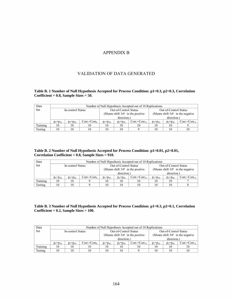
APPENDIX B
VALIDATION OF DATA GENERATED
Table B. 1 Number of Null Hypothesis Accepted for Process Condition: p1=0.3, p2=0.3, Correlation Coefficient = 0.8, Sample Sizes = 50.
Number of Null Hypothesis Accepted out of 10 Replications In-control Status Out-of-Control Status
(Means shift 3σ in the positive direction.)
Out-of-Control Status (Means shift 3σ in the negative
direction.)
Data Set
p1=p10 p2=p20 Corr.=Corr0 p1=p10 p2=p20 Corr.=Corr.0 p1=p10 p2=p20 Corr.=Corr.0 Training 10 10 10 10 10 10 10 10 9 Testing 10 10 10 10 10 9 10 10 10
Table B. 2 Number of Null Hypothesis Accepted for Process Condition: p1=0.01, p2=0.01, Correlation Coefficient = 0.8, Sample Sizes = 910.
Number of Null Hypothesis Accepted out of 10 Replications In-control Status Out-of-Control Status
(Means shift 3σ in the positive direction.)
Out-of-Control Status (Means shift 3σ in the negative
direction.)
Data Set
p1=p10 p2=p20 Corr.=Corr0 p1=p10 p2=p20 Corr.=Corr.0 p1=p10 p2=p20 Corr.=Corr.0 Training 10 10 9 10 10 10 10 10 7 Testing 10 10 9 10 10 10 10 10 8
Table B. 3 Number of Null Hypothesis Accepted for Process Condition: p1=0.3, p2=0.1, Correlation Coefficient = 0.2, Sample Sizes = 100.
Number of Null Hypothesis Accepted out of 10 Replications In-control Status Out-of-Control Status
(Means shift 3σ in the positive direction.)
Out-of-Control Status (Means shift 3σ in the negative
direction.)
Data Set
p1=p10 p2=p20 Corr.=Corr0 p1=p10 p2=p20 Corr.=Corr.0 p1=p10 p2=p20 Corr.=Corr.0 Training 10 10 10 10 10 10 10 10 10 Testing 10 10 10 10 10 9 10 10 10
164

Table B. 4 Number of Null Hypothesis Accepted for Process Condition: p1=0.3, p2=0.3, Correlation Coefficient = 0.8, Sample Sizes = 10.
Number of Null Hypothesis Accepted out of 10 Replications In-control Status Out-of-Control Status
(Means shift 3σ in the positive direction.)
Out-of-Control Status (Means shift 3σ in the negative
direction.)
Data Set
p1=p10 p2=p20 Corr.=Corr0 p1=p10 p2=p20 Corr.=Corr.0 p1=p10 p2=p20 Corr.=Corr.0 Training 10 10 10 10 10 10 10 10 4 Testing 10 10 10 10 10 10 10 10 7
Table B. 5 Number of Null Hypothesis Accepted for Process Condition: p1=0.3, p2=0.3, Correlation Coefficient = 0.2, Sample Sizes = 10.
Number of Null Hypothesis Accepted out of 10 Replications In-control Status Out-of-Control Status
(Means shift 3σ in the positive direction.)
Out-of-Control Status (Means shift 3σ in the negative
direction.)
Data Set
p1=p10 p2=p20 Corr.=Corr0 p1=p10 p2=p20 Corr.=Corr.0 p1=p10 p2=p20 Corr.=Corr.0 Training 10 10 9 10 10 10 10 10 8 Testing 10 10 9 10 10 10 7 10 10
165

REFERENCES
1 Montgomery, D. C., Introduction to Statistical Quality Control (4th edition; John Wiley & Sons, Inc., 2001), pp. 9. 2 Ibid., pp. 9. 3Jackson, J. E., A User’s Guide to Principal Components (John Wiley & Sons, Inc., 1991), pp. 300 – 301. 4 Lowery, C. A. and Montgomery, D. C., “A Review of Multivariate Control Charts,” IIE Transactions, Vol. 27 (1995), pp. 800-810. 5 Jackson (1991), Op. Cit. pp. 21 6 Palm, A. C., Rodriguez, R. N., Spiring, F. A. and Wheeler, D. J., “Some Perspectives and Challenges for Control Chart Methods,” Journal of Quality Technology, Vol. 29, No. 2 (1997), pp. 122 – 127. 7Patel, H. I., “Quality Control Methods for Multivariate Binomial and Poisson Distributions,” Technometrics, Vol. 15, No. 1 (1973), pp. 103-112. 8 Lu, X. S., Xie, M., Goh, T. N. and Lai, C. D., “Control Chart for Multivariate Attribute Processes,” International Journal of Production Research, Vol. 36, No. 12 (1998), pp. 3477-3489. 9 Jolayemi, J.K., “An Optimal Design of Multi-attribute Control Charts for Processes Subject to a Multiplicity of Assignable Causes,” Applied Mathematics and Computation, Vol. 114 (2000), pp. 187-203. 10 Montgomery, D. C., Introduction to Statistical Quality Control (3rd edition; John Wiley & Sons, Inc., 1997), pp. 300 – 301.
11 Ibid., pp. 294 –295. 12 Palm (1997), Op. Cit.
166

13 Palm (1997), Op. Cit. 14 Ryan, T. P. and Schwertman, N. C., “Optimal Limits for Attributes Control Charts,” Journal of Quality Technology, Vol. 29 (1997), pp. 86 – 98. 15 Schwertman, N. C. and Ryan, T. P., “Using Dual np-charts to Detect Changes,” Quality and Reliability Engineering International, Vol. 15 (1999), pp. 317 – 320. 16 Chen, G., “An Improved p Chart Through Simple Adjustments,” Journal of Quality Technology, Vol. 30, No. 2 (1998), pp. 142 – 151. 17 Reynolds, M. R. and Stoumbos, Z. G., “A General Approach to Modeling CUSUM Charts for a Proportion,” IIE Transactions, Vol. 32 (2000), pp. 515 – 535. 18 Reynolds, M. R. and Stoumbos, Z. G., “The SPRT Chart for Monitoring a Proportion,” IIE Transactions, Vol. 30 (1998), pp. 545 – 561. 19 Nelson, Lloyd S., “A Control Chart for Parts-Per-Million Nonconforming Items,” Journal of Quality Technology, Vol. 26, No. 3 (1994), pp. 239 – 240. 20 Su, C. T. and Tong, L. I., “A Neural Network-Based Procedure for the Process Monitoring of Clustered Defects in Integrated Circuit Fabrication,” Computers in Industry, Vol. 34 (1997), pp. 285 – 294. 21 Aparisi, F., “Hotelling T2 Control Chart with Adaptive Sample Sizes,” International Journal of Production Research, Vol. 34, No. 10 (1996), pp. 2853 – 2862. 22 Hotelling, H., Multivariate Quality Control: Techniques of Statistical Analysis, (Eisenhart, Hastay, and Wallis, Eds., New York: McGraw-Hill, 1947) 23 Lowry and Montgomery (1995), Op. Cit. pp.800 - 810. 24 Jackson (1991), Op. Cit. pp. 19. 25 Jackson (1991), Op. Cit. pp. 18, 20 – 25. 26 Wold, H., “Partial Least Square”, Encyclopedia of Statistical Sciences, Vol. 6 (1985), edited by Kotz, Z. and Johnson, N. L. (John Wiley & Sons Inc.) 27 Patel (1973), Op. Cit. pp. 103-112. 28 Lu, Xie, Goh and Lai (1998), Op. Cit. pp. 3477-3489. 29 Jolayemi (2000), Op. Cit. pp. 187-203.
167

30 Jolayemi, J.K., “Convolution of Independent Binomial Variables: An Approximation Method and a Comparative Study”, Computational Statistics & Data Analysis, Vol. 18 (1994), pp. 403 – 417. 31 Jolayami, J.K. and Berrettoni, J.N., “Multivariate Control Charts: An Optimization Approach to Effective Use and Measurement of Performance,” Applied Mathematics and Computational, Vol. 32, No. 1 (1989), pp. 1 – 16. 32 Gibra, I. N., “Economically Optimal Determination of the Parameters of np-Control Charts,” Journal of Quality Technology, Vol. 10, No. 1 (1978), pp. 12 –19. 33 Gibra, I. N., “Economic Design of Attribute Control Charts for Multiple Assignable Causes,” Journal of Quality Technology, Vol. 13, No. 2 (1981), pp. 93 –99. 34 Zorriassatine, F. and Tannock, J. D. T., “A Review of Neural Networks for Statistical Process Control,” Journal of Intelligence Manufacturing, Vol. 9 (1998), pp. 209 – 224. 35 Pugh, G. A., “Synthetic Neural Networks for Process Control,” Computers and Industrial Engineering, Vol. 17, No. 1 – 4 (1989), pp. 24 – 26. 36 Pugh, G. A., “A Comparison of Neural Networks to SPC Charts,” Computers and Industrial Engineering, Vol. 21, No. 1 – 4 (1991), pp. 253 – 255. 37 Guo, Y. and Dooley, K. J., “Identification of Change Structure in Statistical Process Control,” International Journal of Production Research, Vol. 30, No. 7 (1992), pp. 1655 – 1669. 38 Smith, A. E., “ X and R Control Chart Interpretation Using Neural Computing,” International Journal of Production Research, Vol. 32, No. 2 (1994), pp. 309 – 320. 39 Stutzle, T., “A Neural Network Approach to Quality Control Charts From Neural to Artificial Neural Computation,” Proceedings of the International Workshop on Artificial Neural Networks, Malaga-Torrmolinos, Spain, (1995), pp. 1135 – 1141. 40 Cheng, C. S., “A Multi-Layer Neural Network Model for Detecting Changes in the Process Mean,” Computers and Industrial Engineering, Vol. 28, No. 1 (1995), pp. 51 – 61. 41 Chang, S. I. and Aw, C. A., “A Neural Fuzzy Control Chart for Detecting and Classifying Process Mean Shifts,” International Journal of Production Research, Vol. 34, No. 8 (1996), pp. 2265 – 2278. 42 Pugh (1989), Op. Cit. 43 Pugh (1991), Op. Cit.
168
44 Cheng (1995), Op. Cit. 45 Chang and Aw (1996), Op. Cit. 46 Hwarng, H. B. and Hubele, N. F., “X bar Control Chart Pattern Identification Through Efficient Off-Line Neural Network Training, IIE Transactions, Vol. 25, No. 3 (1993b), pp. 27 – 40. 47 Cheng, C. S., “A Neural Network Approach for the Analysis of Control Chart Patterns,” International Journal of Production Research, Vol. 35, No. 3 (1997), pp. 667 – 697. 48 Guh, R. S. and Tannock, J. D. T., “Recognition of Control Chart Concurrent Patterns Using a Neural Network Approach,” International Journal of Production Research, Vol. 37, No. 8 (1999), pp. 1743 – 1765. 49 Guh, R. S. and Hsieh, Y. C., “A Neural Network Based Model for Abnormal Pattern Recognition of Control Charts,” Computers & Industrial Engineering, Vol. 36 (1999), pp. 97 – 108. 50 Chang, S. I., and Ho, E. S., “An Integrated Neural Network Approach for Simultaneous Monitoring of Process Mean and Variance Shifts – a Comparative Study,” International Journal of Production Research, Vol.37, No. 8 (1999), pp. 1881 – 1901. 51 Zorriassatine and Tannock (1998), Op. Cit. 52 Guo and Dooley (1992), Op. Cit. 53 Hwarng and Hubele (1993b), Op. Cit. 54 Cheng (1995), Op. Cit. 55 Cheng (1997), Op. Cit. 56 Hetch-Nelson, R., Neurocomputing, (Addison-Wesley, Reading, MA, 1990). 57 Guo and Dooley (1992), Op. Cit. 58 Hwarng and Hubele (1993b), Op. Cit. 59 Martin, E.B. and Morris, A.J., “Multivariate Statistics and Neural Networks In Process Fault Detection”, IEE-Colloquium-(Digest), No. 079 (1995), pp. 7/1 – 7/8. 60 Wilson, D.J.H., Irwin, G.W. and Lightbody, G., “Neural Networks and Multivariate,” IEE-Colloquium-(Digest), No. 174 (1997), pp. 5/1 – 5/5.
169

61 Wilson, D.J.H. and Irwin, G.W., “Multivariate SPC Using Radial Basis Functions,” UKACC International Conference on Control, Conference Publication No. 455 (1998), IEE. 62 Su, C. T. and Tong, L. I, “A Neural Network-Based Procedure for the Process Monitoring of Clustered Defects in Integrated Circuit Fabrication,” Computers in Industry, Vol. 34 (1997), pp. 285 – 294. 63 Alt, F.B., “Multivariate Quality Control” in Encyclopedia of Statistical Sciences, Vol. 6 (1985), edited by S. Kotz and N.L. Johnson. Jon Wiley & Sons, New York, NY, pp. 110 – 122. 64 Doganaksoy, N., Faltin, F., and Tucker, W.T., “Identification of Out of Control Quality Characteristics in a Manufacturing Environment,” Communications in Statistics – Theory and Methods, Vol. 20 (1991), pp. 2775 – 2790. 65 Hayter, A.J. and Tsui, K.L., “Identification and Quantification in Multivariate Quality Control Problems,” Journal of Quality Technology, Vol. 26 (1994), pp. 197 – 208. 66 Jackson, J.E., “Multivariate Quality Control,” Communications in Statistics – Theory and Methods, Vol. 14 (1985), pp. 2657 – 2688. 67 Mason, R.L., Tracy, N.D., and Young, J.C., “A Practical Approach for Interpreting Multivariate T2 Control Chart Signals,” Journal of Quality Technology, Vol. 29, No. 4 (1997), pp. 396 – 406. 68 Fuchs, C. and Benjamini, Y., “Multivariate Profile Charts for Statitical Process Control,” Technometrics, Vol. 36, No. 2 (1994), pp. 182 – 195. 69 Runger, G.C., Alt, F.B., and Montgomery, D.C., “Contributors to a Multivariate Statistical Process Control Signal,” Communications in Statistics – Theory and Methods, Vol. 25, No. 10 (1996b). 70 Patel (1973), Op. Cit. pp. 103 – 112. 71 Lu, Xie, Goh and Lai (1998), Po. Cit. pp. 3477-3489. 72 Demuth, H. and Beale, M., March 2001, “Chapter 5: Backpropagation,” appears in Neural Network Toolbox for Use with MATLAB (Version 4), 26-27. 73 Goldstein, M. and Dillon, W. R., Discrete Discriminant Analysis (John Wiley & Sons, 1978), pp. 21. 74 James, S. and Wilson, S., “Choosing Between Logistic Regression and Discriminant Analysis”, Journal of the American Statistical Association, Vol. 73, No. 364 (Dec. 1978), pp. 699 – 705.
170

75 Ibid., pp. 699 – 705. 76 Halperin, M., Blackwelder, W. C., and Verter, J. I., “Estimation of the Multivariate Logistic Risk Function: A Comparison of the Discriminant Function and Maximum Likelihood Approaches,” Journal of Chronic Disease, Vol. 24 (1971), pp. 125 – 158. 77 Truett, J., Cornfield, J., and Kannel, W., “A Multivariate of the Risk of Coronary Heart Disease in Framingham,” Journal of Chronic Disease, Vol. 20 (1967), pp. 511 – 524. 78 Gordon, T., “Hazards in the Use of the Logistic Function with Special Reference to Data from Prospective Cardiovasular Studies,” Journal of Chronic Disease, Vol. 27 (1974), pp. 97 – 102. 79 Hosmer, D. W. and Lameshow, S., Applied Logistic Regression (John Wiley and Sons, 1989), pp.127. 80 Ryan, T. P., Modern Regression Methods (John Wiley & Sons, Inc., 1997), pp. 262. 81 Specht, D. F., “Probabilistic Neural Networks,” Neural Networks, Vol. 3 (1990), pp. 109 – 118. 82 Wasserman, P. D., Advanced Methods in Neural Computing (Van Nostrand Reinhold, ITP, 1993), pp. 223. 83 Ryan, P. T., Statistical Methods For Quality Improvement (John Wiley & Sons, Inc., 1989), pp. 104. 84 Woodall, W. H. and Ncube, M. M., “Multivariate CUSUM Quality Control Procedures,” Technometrics, Vol. 27, No. 3 (1985), pp. 285 – 292. 85 Healy, J. D., “A Note on Multivariate CUSUM Procedures,” Technometrics, Vol. 29, No. 4 (1987), pp. 409 - 412. 86 Crosier, R. B., “Mutlivariate Generalizations of Cumulative Sum Quality Control Schemes,” Technometrics, Vol. 30, No. 3 (1988), pp. 291 – 303. 87 Pignatiello, J. J., Jr. and Runger, G. C., “Comparisons of Multivariate CUSUM Charts,” Journal of Quality Technology, Vol. 22, No. 3 (1990), pp. 173 – 186. 88 Woodall and Ncube (1985), Op. Cit. 89 Ong, S. H., “The Computer Generation of Bivariate Binomial Variables with Given Marginals and Correlation,” Communications Statistical – Simulation, Vol. 21, No. 2 (1992), pp. 285 – 299.
171

90 Weintraub, S., Tables of the Cumulative Binomial Probability Distribution for Small Values of p (The Free Press of Glencoe, 1963). 91 Ryan, T. P., Statistical Methods For Quality improvement (John Wiley & Sons, Inc., 1989), pp. 218. 92 Discussion in applied multivariate statistical analysis class (STAT 2310). 93 Montgomery, D. C., Introduction to Statistical Quality Control (4th edition; John Wiley & Sons, Inc., 2001), pp. 295 – 296. 94 Kenett, R. S. and Zacks, S., Modern Industrial Statistics – Design and Control of Quality and Reliability, pp. 148. 95 Devore, J.L., Probability and Statistics for Engineering and the Sciences (4th edition; Wadsworth, Inc., 1995), pp. 512. 96 Law, A. M. and Kelton, W. D., Simulation Modeling & Analysis (2nd edition; McGraw-Hill, 1991), pp. 538 – 539. 97 Montgomery, D. C., Introduction to Statistical Quality Control (4th edition; John Wiley & Sons, Inc., 2001), pp. 167. 98 Cheng, C. S., “A Multi-Layer Neural Network Model for Detecting Changes in the Process Mean,” Computers and Industrial Engineering, Vol. 28, No. 1 (1995), pp. 51 – 61. 99 Cheng, C. S., “A Neural Network Approach for the Analysis of Control Chart Patterns,” International Journal of Production Research, Vol. 35, No. 3 (1997), pp. 667 – 697. 100 Kramer, C. Y. and Jensen, D. R., “Fundamental of Multivariate Analysis Part I. Inference about Means,” Journal of Quality Technology, Vol. 1 (1969a), pp. 120 - 133. 101 Kramer, C. Y. and Jensen, D. R., “Fundamental of Multivariate Analysis Part II. Inference about Two Treatments,” Journal of Quality Technology, Vol. 1 (1969b), pp. 189 - 204. 102 Jackson, J. E., “Quality Control Methods for Several Related Variables,” Technometrics, Vol. 1 (1959), pp. 359 – 377. 103 Jackson, J. E., “Principal Components and Factor Analysis: Part I – Principal Components,” Journal of Quality Technology, Vol. 12 (1981), pp. 201 – 213.
172