A new approach to an

age-old problem:

solving externalities by

incenting workers directly Greer Gosnell, John List and Robert Metcalfe

January 2017

Centre for Climate Change Economics and Policy Working Paper No. 296 Grantham Research Institute on Climate Change and the Environment Working Paper No. 262

This working paper is intended to stimulate discussion within the research community and among users of research, and its content may have

been submitted for publication in academic journals. It has been reviewed by at least one internal referee before publication. The views

expressed in this paper represent those of the author(s) and do not necessarily represent those of the host institutions or funders.

The Centre for Climate Change Economics and Policy (CCCEP) was established by the University of Leeds and the London

School of Economics and Political Science in 2008 to advance public and private action on climate change through innovative,

rigorous research. The Centre is funded by the UK Economic and Social Research Council. Its second phase started in 2013 and

there are five integrated research themes:

1. Understanding green growth and climate-compatible development

2. Advancing climate finance and investment

3. Evaluating the performance of climate policies

4. Managing climate risks and uncertainties and strengthening climate services

5. Enabling rapid transitions in mitigation and adaptation

More information about the Centre for Climate Change Economics and Policy can be found at: www.cccep.ac.uk.

The Grantham Research Institute on Climate Change and the Environment was established by the London School of

Economics and Political Science in 2008 to bring together international expertise on economics, finance, geography, the

environment, international development and political economy to create a world-leading centre for policy-relevant research and

training. The Institute is funded by the Grantham Foundation for the Protection of the Environment and the Global Green Growth

Institute. It has nine research programmes:

1. Adaptation and development

2. Carbon trading and finance

3. Ecosystems, resources and the natural environment

4. Energy, technology and trade

5. Future generations and social justice

6. Growth and the economy

7. International environmental negotiations

8. Modelling and decision making

9. Private sector adaptation, risk and insurance

More information about the Grantham Research Institute on Climate Change and the Environment can be found at:

www.lse.ac.uk/grantham.

A New Approach to an Age-Old Problem:Solving Externalities by Incenting Workers Directly

Greer K. Gosnell, John A. List, and Robert D. Metcalfe∗

January 27, 2017Abstract

Understanding motivations in the workplace remains of utmost import as economiesaround the world rely on increases in labor productivity to foster sustainable economicgrowth. We created a unique opportunity in partnering with Virgin Atlantic Airwaysto test a role for monitoring, performance information, personal targets, and prosocialincentives on fuel efficiency of their captains. We found that monitoring and targetsinduce captains to improve efficiency in all three key flight areas: pre-flight, in-flight,and post-flight. Our study provided the lowest calculated marginal abatement cost perton of CO2, at negative $250 (i.e., $250 savings per ton abated). Methodologically,our approach has implications for climate policy and suggests a new way to combatfirm-level externalities: target workers rather than the firm as a whole.

Keywords: Worker incentives, fuel efficiency, performance feedback, employee effort,information, targets, prosocial incentives, field experiment, aviation

JEL Classification: D01, J3, Q5, R4.

∗Gosnell: London School of Economics and Political Science, List and Metcalfe: University of Chicago. Correspondence toMetcalfe: Department of Economics, Saieh Hall for Economics, 5757 S. University Avenue, Chicago, IL-60637,metcalfe@uchicago.eduAcknowledgments: We thank participants at the 2015 EEE and PPE NBER Summer Institute sessions for excellent remarksthat considerably improved the research, and seminar participants at Columbia University, Dartmouth College, University ofBritish Columbia, UC Santa Barbara, University of Chicago, University of Tennessee, and University of Wisconsin-Madison.Omar Al-Ubaydli, Steve Cicala, Diane Coyle, Paul Dolan, Robert Dur, Robert Hahn, Glenn Harrison, Justine Hastings, DavidJimenez-Gomez, Matthew Kahn, Kory Kroft, Edward Lazear, Steve Levitt, Bentley MacLoed, Jonathan Meer, Kyle Meng,Michael Norton, Sally Sadoff, Laura Schechter, Jessie Shapiro, Kathryn Shaw, Kerry Smith, Alex Teytelboym, Gernot Wagner,and Catherine Wolfram provided remarks that helped to sharpen our thoughts. Thanks to The Templeton Foundation andthe Science of Philanthropy Initiative at the University of Chicago for providing the generous funds to make this experimentpossible, and to the ESRC Centre for Climate Change Economics and Policy and Grantham Foundation for the Protection ofthe Environment for funding the research of Greer Gosnell. Further thanks to the UK Civil Aviation Authority and the pilots’unions who took the time to review and approve of the study objectives and material. A special thanks to those individuals atVirgin Atlantic Airways—especially to Paul Morris, Claire Lambert, Dr. Emma Harvey, and Captain David Kistruck—and RollsRoyce (especially Mark Goodhind and Simon Mayes) for their essential roles in the implementation of this experiment. Theseparties are in no way responsible for the analyses and interpretations presented in this paper. We thank Florian Rundhammerand Andrew Simon for their excellent research assistance.

1 Introduction

Many scientists believe that global climate change represents the most pervasive externalityof our time (Stern, 2006). Perhaps one of the lowest-hanging fruits in combating climatechange is to design firm-level incentive schemes for workers to engage in green behaviors.Given the Environmental Protection Agency estimate that 21 percent of carbon emissionsin the United States are from firms (U.S. Enviromental Protection Agency, 2015), there isundoubtedly much to gain. Yet, very few studies have explored incentive aspects within theworkplace that pertain to sustainability, whether it is shifting work hours to less energy-intensive times of the day or incenting employees to use fewer resources per unit of output.Indeed, when resource use is linked to production costs (as is almost always the case),mitigating the externality has the potential to foster increased profits, providing distinctpossibilities of a win-win scenario.

Consider the transportation sector, and in particular air transportation of humans andcargo. The airline industry is a significant contributor to human welfare, with over threebillion passengers per year and 35% of the value of world trade transported by air (FederalAviation Administration, 2015). However, the global aviation industry is directly responsi-ble for significant health costs among vulnerable population groups (Schlenker and Walker,2016).1 Moreover, excessive fuel use in the industry affects profits—fuel represents an aver-age 33% of airlines’ operating costs (Air Transport Action Group, 2014)—and poses a severerisk to the global environment. Emissions from the air transport sector currently accountfor 3.5-5% of global radiative forcing and 2-3% of global carbon dioxide (CO2) emissions(Penner et al., 1999; Lee et al., 2009; Burkhardt and Kärcher, 2011), deeming the industrya significant force in climate change discussions.2

Technology adoption and market-based instruments continue to appear on the industry’sagenda as primary means to reach its dual goals of carbon neutral growth by 2020 and

1Schlenker and Walker (2016) focus on the effects of network delays in the east coast of the United Stateson congestion at large airports in California to assess health effects from daily variation in air pollution.These effects are presumed to be generalizable across large airports globally and are a consequence of theaviation industry as a whole.

2Past research has shown that the airline industry has also not fully internalized social costs associatedwith crashes (Borenstein and Zimmerman, 1988). Here we highlight yet another means by which the socialcost of the industry is not incorporated into its decision calculus. Nonetheless, demand for air travel isforecasted to increase over the next two decades and, as a result, airline emissions will likely trend upwards(Borenstein, 2011). The future demand for travel will depend on a range of economic factors, and the futurefuel efficiency of the aviation sector will respond to changes in both technology and fuel prices (see Kahnand Nickelsburg, 2016).

1

halving greenhouse gas emissions from 2005 levels by 2050 (see International Civil AviationOrganization, 2013, 2016). Yet, despite large potential to reduce fuel burn from eliminatingoperational inefficiencies (Green, 2009; Singh and Sharma, 2015), almost no research hasbeen undertaken to understand the potential for cost and emissions savings from changes inthe behavior of transport personnel. In fact, we do not know of any research, more generally,on the optimal incentive structure for employees to engage in conservation activities in theworkplace.3

This study takes a strong initial step toward such an understanding by partnering withVirgin Atlantic Airways (VAA) on a field experiment. We observe over 40,000 unique flightsover a 27-month period for the entire population of captains eligible to fly before, during,and after the experiment. In the aviation industry, airline captains maintain a considerableamount of autonomy when it comes to fuel and flight decisions.4 We capitalize on recenttechnological developments that capture detailed flight-level data to measure captains’ fuelefficiency across three distinct phases—pre-flight, in-flight, and post-flight. The pre-flightmeasure (denoted Fuel Load) assesses the accuracy with which captains implement finaladjustments to aircraft fuel load given all relevant factors (e.g., weather and aircraft weight).5

The in-flight measure (denoted Efficient Flight) assesses how fuel-efficiently the captainoperates the aircraft between takeoff and landing. The post-flight measure (denoted EfficientTaxi) provides information on how fuel-efficiently the captain operates the aircraft once onthe ground. The experiment explores the extent to which several experimental treatments—

3Atkin et al. (2015) demonstrate low adoption of waste-reducing technology in a cluster of soccer ballproducers in Pakistan, demonstrating that incentives for employees to use the technology increase uptake.Freeman and Kleiner (2005) study the use of incentive pay on production costs, finding that piece-rate wagesmay increase individual productivity, though not enough to offset the costs associated with monitoring andrequisite managerial policies.

4The “captain”—as opposed to the “first officer”—is the pilot on the aircraft who makes commanddecisions and is ultimately responsible for the flight’s safety. As a rule, captains are the most senior pilots inan airline (see Smith, 2013, for insight into captains’ roles and responsibilities). In the cockpit of a typicalflight from New York to London, there would be one captain and one first officer on board who both engage(more or less equally) in aircraft operations, though the captain is ultimately responsible for all aspects offlight operation. A vast majority of airline captains survive rigorous job market competition to secure theirjobs, investing thousands of hours of training (privately or elsewhere) before obtaining the opportunity tobe considered for a flying career with a major airline. There has been prior research on understanding thedecision making of airline captains under risk, especially through weather conditions (see Gilbey and Hill,2012; Hunter, 2002; Madhavan and Lacson, 2006; Walmsley and Gilbey, 2016; Wiggins et al., 2012).

5Captains do not have much in the way of decision support tools for calculating the correct Fuel Loadapart from pen and a receipt-like sheet of paper—printed in the cockpit prior to departure—indicating thefinal weight of the aircraft. They then use pen and paper to make two calculations using a rule of thumb thatfirst prescribes the amount of additional fuel to load for the flight and subsequently dictates the additionalfuel necessary to carry added fuel.

2

implemented from February 2014 through September 2014—influence captains’ behaviorsalong these dimensions.

The treatments are inspired by a simple principal-agent model characterized by the dis-tinct elements associated with performance-related pay wherein we attempt to understandthe behaviors of VAA captains. Our theoretical model yields predictions on how the actof measurement itself might yield behavioral change, in the spirit of the Hawthorne effectsdescribed in Levitt and List (2011). In addition, the model shows how the distinct elementsof performance-related pay—information, personal targets, and conditional incentives—canmotivate behavioral change. As such, our experimental design revolves around understand-ing how the act of measurement as well as each of these three factors—information aboutrecent fuel efficiency, exogenous performance targets, and prosocial incentives (a donationto the captain’s chosen charity conditional on achieving the target provided)—affect cap-tains’ behaviors from pre-flight to post-flight.6 We are unaware of any previous researchthat estimates the relative magnitude of the discrete elements of performance-related pay,and in particular the impact of targets, on worker productivity in a high-stakes professionalsetting.7

Making use of more than 110,000 observations of the three aforementioned behaviorsacross 335 captains, we find several interesting insights that have the potential to alter con-ventional approaches to motivating employee effort in the workplace while reducing bothoperating costs and environmental damage. First, by simply informing the captains thatwe—i.e., the academic researchers and VAA Fuel Efficiency personnel overseeing the study—are measuring their behaviors on three dimensions, we are able to considerably reduce fuel

6The present study is the first to evaluate the separate elements of performance-related pay (PRP)schemes in a high-stakes setting with experienced professional workers. Many other studies test base payversus PRP; however, PRP has three distinct behavioral elements that might drive a change in behavior:the information, the conditional target, and the incentive itself. Here, these elements are broken down anddistributed across treatment conditions.

7Moreover, it should be noted that the present context is not a typical principal-agent setting, in whichthe principal does not observe effort. Here, the principal has precise measures of effort. However, sincethe highly unionized labor force holds significant bargaining power, the principal faces restrictions againstcontracting on effort (or on output), which is the typical contracting variable in a basic principal-agentmodel. Therefore, the firm is in a “second-best” world requiring use of behavioral incentives as opposed tothe financial incentives in PRP.

3

inefficiency.8 For example, captains in the control group significantly increased the implemen-tation of Efficient Flight and Efficient Taxi by nearly 50 percent from the pre-experimentalperiod. These behavioral changes generated more than 7,700 tons of fuel saved for the airlineover the eight-month experimental period (i.e., $6.1 million in 2014 prices), which translatesto approximately 24,500 tons of CO2 abated.

Second, despite these large Hawthorne effects, we find a significant role for the threeexperimental treatments. The information treatment increases effort for Efficient Taxi, butdoes not increase effort for Fuel Load or Efficient Flight. We find, however, that personal tar-gets increase effort for Efficient Flight and Efficient Taxi, while prosocial incentives increaseeffort across all three dimensions. Furthermore, we find significant differences between theperformance of captains who receive information alone and those who receive targets (withor without incentives), while we do not detect differential effects between the target andprosocial treatment groups. That is, adding a conditional prosocial incentive in the form ofa donation to the captain’s chosen charity does not provide further lift beyond the effects ofproviding a personal target.9

The difference-in-difference treatment effects indicate that the various interventions in-creased implementation of fuel-efficient activities by 1-10 percentage points above the pre-experimental period (i.e., additional to the Hawthorne effect).10 Since the cost of the treat-ments is merely the cost of postage materials (here, $855 per treatment group), the marginalabatement cost (MAC) of the treatments is minuscule, falling between $1.02 and $0.39 perton of carbon saved. However, since the airline benefited from significant cost savings viareduced fuel usage as a result of the interventions, the MAC in this context is approximately-$250 per ton in actuality (using 2014 prices). Such an astonishingly low MAC outperformsevery other reported carbon abatement technology of which we are aware (see Enkvist et al.,

8This pure monitoring effect aligns with agency theory (e.g., Alchian and Demsetz, 1972; Stiglitz, 1975), aswell as with experimental results such as those in Boly (2011) and the observational data from Hubbard (2000,2003). VAA policies precluded the designation of an uninformed control group, so estimates of Hawthorneeffects are based on before-and-after comparisons, as in Bandiera et al. (2007, 2009). Nonetheless, theresults suggest that the data before the experiment was stationary and there was an upward trend oncethe experiment started. Importantly, since all information provided to captains in treatment groups isindividual-specific, we are able to rule out contamination (i.e., spillover effects of information) as a possiblecontributor to the change in behavior exhibited by the control group.

9To our knowledge, we are the first to experimentally estimate the impact of an incentive given to a charityif an employee reaches a certain performance target in his or her job. Our notion of prosocial incentives isdifferent to the social incentives presented in Bandiera et al. (2009, 2010), who demonstrate the manner inwhich social connections in the workplace influence workers’ and managers’ motivations.

10Since there were no upward trends before the experiment began—that is, a Dickey-Fuller test indi-cates that pre-treatment behaviors were stationary—we can be confident that the experiment improved fuelefficiency from business as usual.

4

2007; McKinsey, 2009).11

Third, our experimental design highlights the usefulness of moving beyond short-runeffects in favor of understanding long-term embedded behavior change. We find that thelargest effects for Fuel Load and Efficient Flight arise in the middle months of the experiment,while the treatment effect for Efficient Taxi is consistently high throughout the experiment,demonstrating no evidence of treatment effect decay during the study period. Interestingly,across all three treatments, we find the largest effects for the behavior that is the easiest tochange (Efficient Taxi). Once the experiment finishes, however, we find that treated captains’effort reverts to post-experiment baseline levels (i.e., equivalent attainment to the controlgroup) for Fuel Load and Efficient Flight, while the treatment effects remain but attenuatefor Efficient Taxi. With regards to persistence of the Hawthorne effect, the post-experimentbaseline remains considerably improved from the pre-experiment baseline, perhaps indicatingthat monitoring induces captains to make low-effort efficiency improvements that are quicklyand easily habituated.12

Finally, the research design allows us to demonstrate welfare benefits pertaining to theemployees. Careful analysis of data from a post-study debrief survey reveals that captains’job satisfaction is positively influenced by prosocial incentives and fuel performance.13 Cap-tains in the prosocial treatment group report a job satisfaction rating 6.5% higher thancaptains in the control group (p<0.1). Moreover, for captains receiving targets or proso-cial incentives, every additional target met (out of 24 opportunities in total) increases jobsatisfaction by 1%, on average. This improvement in job satisfaction demonstrates the fea-sibility of nudging agents to increase effort without imposing any welfare loss. Additionally,it suggests that the experiment resulted in a “win-win-win” in that it reduced the firm’s op-erating costs, curtailed globally harmful greenhouse gas emissions, and improved employeesatisfaction.

The research findings are relevant for academics, businesses, and policymakers alike. Foracademics, the theory and experimental results hold implications for environmental, labor,and public economics. For example, there exist movements within both applied economics

11The most cost-effective abatement strategy according to McKinsey (2009) is to switch residential lightingfrom incandescent bulbs to LED bulbs at a MAC of approximately -165 Euro, or about -$177.

12An alternative interpretation to the Hawthorne effect could be that the captains now learn that the firmvalues fuel efficiency (a value that captains likely share). This interpretation relates to the work by Bloomand Van Reenen (2007) and Bloom et al. (2014) on the impact of ‘soft’ management styles and structureson worker productivity. Our experimental design does not allow us to parse out these two interpretations ofthe Hawthorne effect.

13We measured job satisfaction in the debrief survey since it is a metric commonly used in the airline andother industries to assess the well-being of employees.

5

(“X-efficiency”; see Leibenstein, 1966) and environmental economics (the “Porter Hypothe-sis”; see Porter and van der Linde, 1995) arguing that substantial “free gains” exist withinfirms. The premise is a behavioral one: rather than modeling firms as fully aware andunderstanding of all extant means to maximize resource efficiency—thereby exhausting allcost-efficient measures at each moment in time—this approach considers the firm as a compo-sition of networks of boundedly rational individuals burdened by problematic principal-agentincentive conflicts (Leibenstein, 1966; Perelman, 2011). To support this view, a survey ofevidence argues that a typical firm operates at 65% to 97% efficiency (Button and Weyman-Jones, Button and Weyman-Jones), though much of this evidence is based on observationaldata and does not assess impacts based on a true counterfactual. The causal estimates fromour field experiment complement this environmental and behavioral research by moving ina hitherto unconsidered direction: rather than focus on capital improvements or researchand development, we explore efficiency effects of incenting labor directly during their normalcourse of work. For labor economists considering principal-agent settings, our study sug-gests that allowing the agent flexibility to achieve goals might be a key trigger in enhancingeffort profiles, and that such goals’ conditionality may have an important role to play in theefficacy of performance-related pay.

For businesses and policymakers, we present a novel and promising approach to combat-ing firm-level externalities: design appropriate incentives for workers. More narrowly, thestudy provides practical and cost-effective fuel solutions for the air transport industry. Ourempirical approach lends itself naturally to related tests across other sectors of the economy.By making use of our theoretical framework to guide experimental treatments in the field,businesses and policymakers can learn not only what works, but also why it works. Thisunderstanding will provide decision-makers with a more effective toolkit to advance efficientpolicies and procedures.

Our results also hold implications for global climate policy. We find that companies maynot be at their production possibilities frontier due to internal frictions, such as managementconstraints imposed by unionization. An optimal carbon tax may not result in sociallyoptimal emissions production in the presence of such constraints. Interventions such asthose presented in this paper can partially alleviate the externalities associated with suchconstraints, but a carbon tax policy may require a dismantling of said frictions in order toachieve optimal emissions levels. It would be wise for climate economists and policymakersto acknowledge that in many industries where frictions exist (such as the transport sector),the optimal policy instrument will likely not obtain the first-best outcome. Future research

6

should aim to address the gap that such frictions drive between theoretical optima andoutcomes in practice.

The remainder of the paper is structured as follows. Section 2 provides contextual back-ground, a sketch of the theory of captain behavior, and the experimental design. Section 3presents the experimental results. Section 4 provides a discussion related to policy implica-tions and related avenues for future research.

2 Background, Theory, and Experimental Design

2.1 Background: Captains’ Behavior and Fuel Efficiency

In 2012, we began discussions with VAA to partner on a field experiment with the aim of un-derstanding behavioral components of fuel usage without adversely affecting safety practicesor job satisfaction.14 We developed a theoretical framework and a field experiment (detailedfurther below) that allowed us to remain within institutional constraints while maintainingthe integrity of lending theoretical insights to the experimental data. We agreed to providemonthly tailored feedback to 335 airline captains—the entire eligible captain population ofVAA—from February 2014 through September 2014. Importantly, all eligible VAA captainswere included in the experiment—in either control or treatment. Since participants wereaware that they were part of an experiment, our field experiment should be considered aframed field experiment in the parlance of Harrison and List (2004). Yet, unlike any otherframed field experiment of which we are aware, we are estimating a parameter devoid of selec-tion bias since all captains are experimental subjects. In this way, our behavioral parameterof interest shares much with that estimated in a natural field experiment (see Al-Ubaydliand List, 2015).

While many of the captains’ choices are important in terms of fuel efficiency outcomes,we worked with VAA to identify three primary measurable levers to change behavior for thepurpose of this study.15 The first lever is a pre-flight consideration, which VAA refers to as theZero Fuel Weight (ZFW) adjustment. Approximately 90 minutes before each flight, captains

14The study is a component of Change is in the Air, VAA’s wider sustainability initiative (seehttp://www.virginatlantic.com/gb/en/sustainability.html).

15The captains in our study have absolute authority to make all fuel-related decisions. They range inexperience and fly long-haul flights on various aircraft types (Airbus 330-300, Airbus 340-300, Airbus 340-600, Boeing 744-400). We include a map of destinations in Figure 1. All operations to Aberdeen andEdinburgh are VAA Little Red operations (i.e., branded VAA flights operated by a third party) and wereexcluded from the analysis. In April 2015, VAA removed its service to Cape Town; this route change tookplace subsequent to the period covered in our dataset.

7

utilize flight-specific flight plan information (e.g., expected fuel usage, weather, and aircraftweight) in conjunction with their own professional judgment to determine initial fuel uptake,which usually corresponds to approximately 90% of the anticipated fuel necessary for theflight. This amount is fueled into the aircraft simultaneous to the loading of passengers andcargo. Near to completion of passenger boarding and cargo/baggage loading, the pilots—nowon the flight deck—receive updated information regarding the final weight of the aircraft andmay adjust the fuel on the aircraft accordingly. The information they receive from FlightOperations includes a ZFW measure, which indicates the weight of the aircraft with therevenue load (i.e., passengers and cargo), as well as the Takeoff Weight (TOW), whichincludes both revenue load and fuel.

Captains then perform a ZFW calculation in which they first calculate the amount bywhich they should increase or decrease fuel load based on the final ZFW—a formula thatis standard across the airline industry. If they have decided to increase the fuel load, theysubsequently compute a second iteration to account for the additional fuel necessary to carrythe fuel that they have decided to add to the aircraft. If the amount of fuel already on theaircraft is sufficient according to these calculations, the captain may choose not to add anyadditional fuel.

For mnemonic purposes, rather than use ZFW we denote this binary outcome variableas Fuel Load. Fuel Load indicates whether the double iteration calculation has been per-formed and the fuel level adjusted accordingly. We deem the captains’ behavior successfulif their final fuel load is within 200 kg of the “correct” amount of fuel as dictated by thecalculation.16,17 This allowance prevents penalizing captains for rounding and slight over- orunder-fueling on the part of the fueller while providing measurable targets for captains intwo of our treatment groups. According to our partner airline, accurate Fuel Load adjust-ment should ideally be performed on every flight regardless of circumstances, which wouldcorrespond to 100% attainment for the performance metric provided.

The second lever is an in-flight consideration: Efficient Flight. The Efficient Flight metriccaptures whether captains (and their co-pilots) use less fuel during flight than is allotted in

16Virgin Atlantic deemed 200 kg a reasonable buffer to allow for rounding in the zero fuel weight calculationas well as marginal errors in fuelling on the part of the aircraft fueller. The results are robust to upward anddownward adjustments of this buffer by 50 kg.

17Using data from a major U.S. airline, Ryerson et al. (2015) estimate that 4.5% of fuel burned on anaverage flight is attributable to carrying unused fuel, and that more than 1% of fuel burned on an averageflight is due to addition of contingency fuel “above a reasonable buffer”. Although they claim that the airlineloads fuel conservatively, they estimate that small changes in fuel loading procedure can save an amountof fuel each year equivalent to that consumed by 4760 flights on mid-sized aircraft for a savings of 153,314metric tons of CO2

8

the updated flight plan.The flight plan is updated subsequent to decisions made on Fuel Loadso that decisions regarding the first metric do not affect one’s ability to meet this in-flightmetric. We use this metric to understand whether captains have made fuel-efficient choicesbetween takeoff and landing. This measure incorporates several in-flight behaviors thataugment fuel efficiency, such as requesting and executing optimal altitudes and shortcutsfrom air traffic control, maintaining ideal speeds, optimally adjusting to en route weatherupdates, and ensuring efficient aerodynamic arrangements with respect to flap settings aswell as takeoff and landing gear. The Efficient Flight metric affords captains the flexibilityto achieve the target while using professional judgment to ensure that safety remains thefirst priority. Under some uncommon circumstances, operational requirements dictate thatcaptains sacrifice fuel efficiency (and VAA accepts the captains’ decisions as final), so wewould not expect even a “model” captain to perform this metric on 100% of flights, thoughthe metric should be attainable on a vast majority of flights. In our analysis, Efficient Flightequals 1 if the captain does not exceed the projected fuel use for that flight (adjusted foractual TOW), and 0 otherwise.18

The final lever—reduced-engine taxi-in (Efficient Taxi or Efficient Taxiing, hereafter)—occurs post-flight. Once the aircraft has landed and the engines have cooled, captains maychoose to shut down one (or two, in a four-engine aircraft) of their engines while theytaxi to the gate, thereby decreasing fuel burn per minute spent taxiing. Captains meetthe criteria for this metric if they shut down (at least) one engine during taxi-in.19 Aswith Efficient Flight, there are circumstances under which the airline would not expect orprescribe the implementation of Efficient Taxi. Obstacles include geographical constraints(e.g., the placement or layout of the runway) and the complexity of the taxi route (e.g.,number of stops, turns, or cul-de-sacs). Still, the metric should also be attainable on a vastmajority of flights, and obstacles to implementation are uncorrelated with treatment.

2.2 Theoretical Sketch of Captains’ Behavior

We model an airline captain’s choices using a static game of a principal-agent model thatdetermines a captain’s chosen effort in a given period (for parsimony, we briefly sketch the

18Note that it was essential to create binary metrics for Fuel Load and Efficient Flight so we could assigntargets to captains in the targets and prosocial incentives group.

19Fuel savings from Efficient Taxi depend on scheduling and delays as savings are accrued on a per-minutebasis. Fuel savings also depend on aircraft type and only begin to accrue after engines have cooled, whichtakes 2-5 minutes from touch down. Savings per minute for aircraft operated within the study are as follows:12.5 kg (Boeing 744-400, Airbus 330-300), 8.75 kg (Airbus 340-600), and 6.25 kg (Airbus 340-300).

9

model here and provide details in Appendix II). The tasks consist of the aforementionedpre-flight to post-flight fuel usage metrics. Captains observe their own effort and a signalof optimal fuel usage; the signal is noisy unless the captain receives information. Captains’perspectives on fuel usage and their fuel-relevant decisions are rooted in their own experiencesand preferences and are conditional on contextual (i.e., flight- and day-specific) factors.

To account for the various potential sources of motivation triggered under performance-related pay, captains in our model maximize a utility function that comprises the followingadditively separable components: utility from wealth, utility from job performance, andutility from charitable giving, as well as disutility from effort exertion and disutility fromsocial pressure. The model has the standard prediction from the first-order conditions thatthe captain will expand effort until its marginal cost equals the marginal utility gained fromthe associated decrease in fuel usage. This prediction occurs on several dimensions, such asutility from job performance, utility from giving to a charity, as well as disutility from socialpressure (a la DellaVigna et al., 2012).

Although our base model follows DellaVigna et al. (2012), we extend the model to in-corporate a reference-dependent component to capture the effects of exogenous performancetargets devoid of conditional incentives. In line with existing theories of reference depen-dence, we posit that a change in one’s personal expectations from the status quo to animproved outcome can boost performance and, consequently, utility. We therefore introducefeedback to employees providing non-binding targets—i.e., focal points for attainment ofthe three fuel-relevant behaviors—that encapsulate reference-dependent preferences.20 Weexpect utility from job performance to increase for those who meet their targets. As in theKöszegi and Rabin (2006) model of reference-dependent preferences, we assume individu-als are loss averse so that performing below the target level will cause more disutility thanexceeding the target level will benefit the individual.

The notion that prosocial incentives can motivate behavior change is rooted in theories ofpure and impure altruism (Becker, 1974; Andreoni, 1989, 1990). Pure altruism requires thatindividuals derive utility from the provision of a public good. Impure altruism posits thatindividuals gain utility from the act of giving itself, so that an individual whose altruism iscompletely impure will provide the same dollar value toward the public good regardless ofthe provision of others. Both pure and impure altruism provide positive utility to (altruistic)

20There is a rich psychology literature on goal setting. Heath et al. (1999) present evidence that goals actas reference points inducing loss aversion and diminishing sensitivity in a manner consistent with ProspectTheory (see also Locke and Latham, 2006). Psychology studies do not exist that address the complex andhigh-stakes field environment in which our experiment takes place.

10

economic agents, and we assume that individuals are characterized by some combination ofthe two (we do not attempt to distinguish between them in the experiment). This character-ization provides a prediction that altruistic motivations combined with prosocial incentiveswill augment fuel efficiency.

In equilibrium, captains choose the corresponding effort level that satisfies the first-orderconditions. These choices lead to several propositions.21 First, if social pressure is important,then captains in the control group will improve their fuel efficiency due to the enhancedscrutiny of their fuel usage. Second, providing information to captains will cause them toincrease (weakly decrease) their effort if estimated fuel usage is lower (higher) than theiractual fuel usage. The intuition is that the relationship between captains’ estimated fuelusage and their actual fuel usage importantly determines their utility from job performance.For example, informing captains that they are fuel inefficient will induce captains to exertgreater effort if they derive disutility from consuming more fuel than their estimated usage.Alternatively, if their fuel usage is deemed lower than their estimated usage, they may exertless effort since effort is costly.

Third, targets set above pre-study fuel use will cause captains to weakly increase theireffort. Captains will increase their effort if the marginal gain from the associated decreasein fuel usage due to the target is greater than the marginal cost of effort. Alternatively,captains will not increase their effort if the marginal cost of effort is larger than the marginalgain from the associated decrease in fuel usage in the job performance parameter. Fourth,conditional donations to charity will increase effort if captains’ altruism is strictly positiveand will not affect their effort otherwise. Fifth, of the three dimensions to lower fuel usage—pre-flight, in-flight, and post-flight—captains will choose to increase their effort the most intasks for which the targets are least costly to meet (i.e., Efficient Taxi).

In light of these predictions, we design a field experiment to measure how behaviors re-lated to fuel usage are affected by: i) information about recent fuel efficiency, ii) informationabout target fuel efficiency, and iii) a donation to a chosen charity conditional on achievingthe target efficiency. To our knowledge, we are the first to perform a large-scale field experi-ment on firm employees in a high-stakes professional labor setting (where the average salary

21These propositions would remain unchanged in a multi-tasking model setup.

11

of a captain is roughly $175,000-$225,00022).23 In doing so, we overcome prominent labormarket frictions in the airline industry by implementing interventions that do not changecontracts of the captains.24 We outline the field experimental design below.

2.3 Experimental Design

In accordance with our theoretical model, the field experiment focuses on three main be-havioral motivations for optimizing fuel use: personalized information, performance targets,and prosocial incentives. The three treatments centered upon three behaviors relevant tofuel use: Fuel Load, Efficient Flight, and Efficient Taxi. Respectively, these three behaviorsallow us to capture captains’ behavior before takeoff, during the flight, and after landing.Airline captains did not receive detailed information relating their decision-making to theirfuel efficiency prior to this experiment (consistent with both airline and industry standards).Recent advances in aircraft data collection allow us to obtain precise data to inform captainsof the link between their effort and their efficiency.

We provided accurate monthly feedback to three treatment groups over the course of eightmonths across 335 captains; a control group did not receive any feedback but was aware that

22This salary range is based on information updated in June 2015:http://www.pilotjobsnetwork.com/jobs/Virgin_Atlantic.

23There is a growing literature surrounding field labor economics, but most experiments have focused onsimple tasks (List and Rasul, 2011; Bandiera et al., 2011; Levitt and Neckermann, 2014). Using a before-and-after design within the same company, Bandiera et al. (2007, 2009, 2010) demonstrate the effects ofmanagerial compensation and social connections in the workplace on worker productivity and selection in thefruit picking industry. Shearer (2004) finds that piece-rate wages improve worker productivity in tree plantingrelative to fixed-rate wages; Lazear (1999) finds similar incentive effects of piece-rate wages in an observationalstudy of automobile glass installers. Field experiments on the impact of retail store-level tournaments onsales show mixed results (Delfgaauw et al., 2013, 2014, 2015), while a quasi-experiment showed that simplyinforming warehouse employees of relative wage standing permanently improved productivity (Blanes i Vidaland Nossol, 2011). One exception to such task simplicity is Gibbs et al. (2014), who analyze the effects ofa rewards program on innovation at a large Asian technology firm in a field experimental setting. Theyfind that providing rewards for idea acceptance substantially increases the quality of ideas submitted. Inan envelope-stuffing experiment, Al-Ubaydli et al. (2015) find that quality is actually higher under piece-rate wages (contrary to predictions from economic theory), speculating a role for beliefs about employers’ability to monitor. In an artefactual field experiment with bicycle messengers, Burks et al. (2009) findthat performance-related pay reduces cooperation in a prisoner’s dilemma game relative to a flat wage.There has been some research by Rockoff et al. (2012) that demonstrates that simple information on teacherperformance to employers (i.e., school principals) can improve productivity in schools, increase turnover forteachers with low performance estimates, and produce small test score improvements.

24While a standard principal-agent model would prescribe the use of contracted performance-related payto align captains’ fuel use incentives with those of the airline, the airline workforce is a different labor marketto most due to the high skill requirements (and often government safety certifications) necessary to enter thisparticular labor force. See Borenstein and Rose (2007) for a further discussion of the labor market frictionsof the aviation industry.

12

their fuel usage was being monitored.25 Printed feedback reports with information from theprevious month’s flights were sent to the home addresses of treated captains, so that captainsreceived their first feedback report in mid-March 2014 and their final feedback report in mid-October 2014. The three experimental treatments can be summarized as follows:

Treatment Group 1: Information. Each feedback report details the captain’s perfor-mance of the three fuel-relevant behaviors for the prior month (see Figure A1 in AppendixIII). Specifically, the feedback presents the percentage of flights flown during the precedingmonth for which the captain successfully implemented each of the three behaviors. For in-stance, if a captain flew four flights in the prior month, successfully performing Fuel Load andEfficient Taxi on two of the flights and Efficient Flight on three of the flights, his feedbackreport would indicate a 50% attainment level for the former behaviors and a 75% attainmentlevel for the latter.

Treatment Group 2: Targets. Captains in this treatment group received the sameinformation outlined above but were additionally encouraged to achieve personalized targetsof 25% above their pre-experimental baseline attainment levels for each metric (capped at90%; see Figure A2 in Appendix III). The targets were communicated to these captains priorto the start of the experiment. An additional box is included in the feedback report to providea summary of performance (i.e., total number of targets met). If at least two of the threetargets were met, captains were recognized with an injunctive statement (“Well Done!”)and encouraged to continue to fly efficiently the following month. If fewer than two targetswere met, captains were encouraged to fly more efficiently to reach their targets. Captainswere not rewarded or recognized in any public or material fashion for their achievements.

Treatment Group 3: Prosocial Incentives. In addition to the information and25In keeping with VAA’s culture of transparency, carefully crafted study information sheets were posted

to captains’ home addresses on January 20, 2014. These information sheets guaranteed captains of theanonymity of their data, assured them that the study held no implications for their salaries or careerprospects, and indicated that the study was not a step in the direction of competitive league tables. Forinstance, the initial letter sent to all (treatment and control) captains in January 2014 included the followingstatements (emphasis included): “This is not, in any way, shape or form, an attempt to set up a‘fuel league table’, or any attempt at moving in the direction of a fuel league table. It is an in-dependent research project to see whether information provided in different ways affects individual decisions.All data gathered during this study will remain anonymous and confidential... Again, we would like tostress that Captains’ anonymity will be maintained throughout the study; whilst somebody in Flight Ops Ad-min has to correlate which Captain gets which letter, Flight Operations Management will have no visibility ofwhich Captain is in which Group, and who is doing what in response to which information. Information willbe sent to all Captains in the active study groups. What you choose to do with that information is entirelyup to you.” Additionally, captains in treatment groups received a notification of their assigned treatmentgroup with a sample feedback form, including the appropriate targets for captains in Treatment Groups 2and 3, which were posted on January 27, 2014, five days prior to the first day of monitoring.

13

targets provided to captains in treatment group 2, those in the prosocial treatment groupwere informed that achieving their targets would result in donations to charity (see FigureA3 in Appendix III). Specifically, for each target achieved in a given month, £10 was donatedto a charity of the captains’ choice on their behalves.26 Therefore, captains in this treatmentgroup each had the opportunity to donate £30 ($49) per month for a total of £240 ($389) totheir chosen charity over the course of the eight-month trial. Captains were reminded eachmonth of the remaining potential donations that could result from realizing their targets inthe future. To our knowledge, ours is the first experimental study to use performance-basedcharitable incentives to increase employee effort in a high-stakes labor setting.27 Table 1outlines the treatments.

The “build-on” experimental design allows us to assess whether there are additionalmarginal benefits of prosocial incentives beyond sole provision of information and personaltargets, the latter of which have an extremely low marginal cost to the principal.28 Withinthe experimental context, organizational structures and captains’ contracts were intention-ally left unchanged, though we recognize that these factors likely play an important rolein determining productivity and efficiency.29 Importantly, the experimental feedback andincentive schemes permit flexibility for workers to achieve their goals. In this way, ratherthan mandate or incent a particular course of action, we follow a more adaptable approachthat permits gains to be had in accord with the captains’ personal and professional discretion.

26When captains in the prosocial treatment group were informed of their assignment to treatment, theywere offered the opportunity to choose one of five diverse charities to support with their charitable incentives:Free the Children, MyClimate, Help for Heroes, Make A Wish UK, and Cancer Research UK. Eighteencaptains selected a charity by emailing the designated project email address, and 67 captains who did notactively select a charity were defaulted to donate to Free the Children. Captains could choose to remainanonymous, otherwise exact donations were attributed to each individual (identified by their first initial andlast name).

27For related work, see Tonin and Vlassopoulos (2010) for a field experiment where university students’pure and impure altruism are assessed via a data entry task with charitable incentives. Additionally, seeTonin and Vlassopoulos (2014) for an online experiment as well as Imas (2014) and Charness et al. (2014)for lab experiments on the effect of charitable incentives on effort, and Anik et al. (2013) for a field study ofunconditional charitable bonuses. Elfenbein et al. (2012) show that sellers who tie products to a charitabledonation may be deemed more trustworthy by consumers. Relatedly, field experimental research into uncon-ditional gifts is a burgeoning area of research—see Gneezy and List (2006); Bellemare and Shearer (2009);Hennig-Schmidt et al. (2010); Englmaier and Leider (2012); Kube et al. (2012); and Cohn et al. (2015).

28The closest research to this “free lunch” approach is embodied in the field experiments of Grant andGino (2010); Kosfeld and Neckermann (2011); Bradler et al. (2013); Chandler and Kapelner (2013); Gubleret al. (2013); Ashraf et al. (2014); Ashraf et al. (2014); and Kosfeld et al. (2014).

29See Nagin et al. (2002); Hamilton et al. (2003); Karlan and Valdivia (2011); Bandiera et al. (2013);Bloom et al. (2013); Karlan et al. (2015); Bloom et al. (2015). Our context is the single firm experimentalsetting in the insider econometrics approach (Shaw, 2009).

14

2.4 Further Experimental Details

2.4.1 Randomization

To randomize captains across the four groups, the pre-experimental data (September-November,2013) were first blocked on five dummy variables that captured whether subjects were aboveor below average for: i) number of engines on aircraft flown, ii) number of flights executedper month, and iii) attainment for the three selected fuel-relevant behaviors. The former twovariables were those that proved significant in determining the selected outcome behaviors inpreliminary regressions, while the three target behaviors are our main dependent variables.Once blocked, subjects in each block were randomly allocated to one of the four study groupsthrough a matched quadruplet design. To ensure that individual-specific observable char-acteristics are balanced across groups, we performed balance tests for seniority, age, trainerstatus, and trusted pilot status (see Table 2) as well as flight plan fuel (i.e., as a proxy foraverage flight distance), average number of engines on aircraft flown, flying frequency, andthe three targeted behaviors (see Table 3). In short, an exploration of all available aspects ofcaptain and flight data reveals that the randomization was successful in that the observablesare balanced across the four experimental conditions.

2.4.2 Communication with captains

Two weeks prior to the study start date of February 1, 2014, all captains were informedthat VAA would be undertaking a study on fuel efficiency as part of its Change is in theAir sustainability initiative. The initial letter outlined the three behaviors to be measuredand the possible study groups to which the captains may be randomly assigned. Captainsin treatment groups were to receive letters the following week to inform them of what toexpect in the coming months. In the final week of January 2014, letters were sent to alltreated captains informing them of the intervention to which they had been assigned. Theletter included a sample feedback report and contained the individual’s targets if he hadbeen assigned to the targets or prosocial group.

From February 1, 2014 to October 1, 2014, we gathered all flight-level data on a monthlybasis for each captain and mailed a feedback report to the home address of each treatedcaptain. Captains were encouraged to engage with the material and send any questions toan email address created specifically for study inquiries. Once the experiment was complete,

15

we sent treated captains a debrief letter informing them of their overall monthly resultswith respect to their targets (if in the targets or prosocial treatment groups) and their totalcharitable donations (if in the prosocial incentives treatment group). All (treatment andcontrol) captains were informed that a follow-up survey would be sent to their companyemail addresses in early 2015.30

2.4.3 Sample

Our data consists of the entire eligible universe of VAA captains (N = 335), of which 329 aremale and 6 are female.31 Of the debrief survey respondents, 97 classified their training asmilitary and 102 as civilian (the remaining declined to state). Eleven captains are “trustedpilots” who were selected for consultation regarding study feasibility and communications,and 62 captains are “trainers” who are responsible for updating and training captains andfirst officers with the latest flight techniques. Captains ranged from 37 to 64 years of age,where the average captain was 52 years old and had been an employee of the airline forover 17 years when the study initiated. Captains in the sample flew five flights per monthon average, where the captain flying most averaged almost eight flights per month and thecaptain flying least averaged just over two flights per month.32

The resulting dataset consists of 42,012 flights and 110,489 observations of fuel-relatedbehavior from January 2013 through March 2015 for the captains sampled.33 Among othervariables, we observe fuel (kg) onboard the aircraft at four discrete points in time: departurefrom the outbound gate, takeoff, landing, and arrival at the inbound gate. In addition, we ob-serve fuel passing through each of the aircraft’s engines during taxi, which provides a precise

30The follow-up survey was designed and administered by the academic researchers alone. Again, captainswere assured that data from their responses would be used for research purposes only, that their responseswould remain anonymous, and that VAA would not be privy to individual-level information provided bysurvey respondents.

31A handful of VAA captains who were on leave for personal reasons or were fulfilling duties outside oftheir usual obligations were excluded from the sample.

32During the study, Rolls Royce (Controls and Data Services) provided monthly data to VAA. We (theacademic researchers) almost always received access to the data within two weeks of the start of the month,and feedback reports were compiled and returned to VAA within 24 hours to be postmarked the following day.VAA subsequently provided post-study data (October 2014 through March 2015) for persistence analysis.

33We exclude domestic and repositioning flights from our analysis. Efficient Taxiing data is physicallystored on QAR cards inside the aircraft, which are removed every 2-4 days to pull data. These cards cancorrupt or overwrite themselves, and also can reach full memory capacity before being removed. Therefore,data capture for Efficient Taxi is not complete—exactly 37% of flights are missing data for this metric. Thereason for the missing data is purely technical and cannot be influenced by captains. We regress an indicatorvariable of missing Efficient Taxi data on treatment indicators and find no statistically significant relationshipat any meaningful level of confidence (individual and joint p > 0.4). Consequently, this phenomenon shouldnot affect results beyond reducing the power of estimates.

16

measure of fuel burned while on the ground. We also observe flight duration, flight plan vari-ables (i.e., expected fuel use, flight duration, departure destination, and arrival destination),and aircraft type. We control for several flight-level variables—e.g., ports of departure andarrival, weather on departure and arrival, whether the aircraft had just received maintenance(e.g., belly wash, engine change), and aircraft type—as well as captain-level time-varying ob-servables such as current contracted work hours and whether the captain had attended theannual Ops Day training.

3 Results

3.1 Main Results

Table 4 and Figures 2a-2c provide a summary description of captains’ performance of thefuel-efficient behaviors before and during the experimental period. In accordance with thebalance checks using data from September through November of 2013 in Tables 2 and 3, thesummary statistics from January 2013 through January 2014 (i.e., Table 4, ’Before Experi-ment’) provide assurance that the pre-experimental behavioral outcomes are balanced acrossvarious study groups. For instance, roughly 42% of flight observations were characterizedby efficient Fuel Load in the 13 months before the experiment started (Table 4, Row 1),and attainment within the experimental groups is approximately 41-43%. Likewise, figuresare similar for Efficient Flight (roughly 34%) and Efficient Taxi (roughly 33%). None of thedifferences across groups are statistically significant at conventional levels.

A second noteworthy insight is the large difference in behaviors before and during theexperiment for the control captains, leading to our first formal result:

Result 1. Captains in the control group change their behavior considerably after they areinformed that they are being monitored.

Preliminary evidence for this result is contained in Column 1 of Table 4. For example,whereas control captains met the Efficient Flight threshold on 31.1% of flights before theexperiment, they met the threshold on 47.6% of flights during the experiment (p < 0.01).Likewise, control captains implemented Efficient Taxi on 50.7% of flights during the ex-periment compared to 35.2% before the experiment (p < 0.01). While the results are noteconomically large for the Fuel Load variable, they again point in the same direction as theother two measures: after the control captains become aware that their actions are being

17

measured, they increase the precision of their fuel load (44.3% versus 42.1% of flight obser-vations; p < 0.05). Figures 2a-2c provide a visual summary of this result, and reinforce thesubstantial difference in captains’ behavior once the experiment began.34

While these summary statistics are certainly consistent with Result 1, they do not accountfor the data dependencies that arise from each captain’s provision of more than one datapoint nor any trends in the pre-experimental period. To control for the panel nature of thedata set, we estimate a regression model of the form:

EfficientBehaviorit = α + Expit · Titβ +Xitγ + ωi + eit

where EfficientBehaviorit equals one if captain i performed the fuel-efficient behavior on flightt, and equals zero otherwise; Expit describes the experimental period; Tit represents a vectorwith indicator variables for the three treatments; Xit is a vector of control variables; and ωiis a captain fixed effect. We include all available and relevant flight variables as controls,which include weather (temperature and condition) on departure and arrival, number ofengines on the aircraft, airports of departure and arrival, engine washes and changes, andairframe washes. Additionally, we control for captains’ contracted flying hours and whetherthe captain has completed training.35

We estimate the above difference-in-difference model specification for each of the fuel-efficient activities using panel data from January 2013 through September 2014, and we treatthe first day of the experiment as February 1, 2014, when monitoring of captains begins.Three different empirical approaches yield qualitatively similar results: linear probabilitymodel (LPM), probit, and logit. For ease of interpretation, we only present the results ofthe LPM in Table 5.36 Robust standard errors are clustered at the captain level. As analternative, we present Newey-West standard errors for the same model.

We first note the coefficient estimate of the experimental period (“Expt”), which providesa measure of how the control group changed behavior over time. We find a staggering effect:the control group increased their implementation of Efficient Flight by 14.4 percentage points

34Data on pre-experiment trends were largely flat with noise, ruling out that this result is simply revealinga general trend of behaviors over time (see Table A1 of Appendix I).

35There are various types of training courses, foremost of which is time spent in the simulator (majorityof training) in which captains must pass assessments; we do not have accurate data on these trainings. Weinstead control for attendance at the two-day “Ops Day” seminar, a gathering of small groups of pilots(approximately 20 per training) for briefing that includes discussion of the goals and directions of the airlineand presentations from various teams, with some informal training for pilots.

36Results of probit and logit specifications are available upon request.

18

(46.3% effect, 0.31 standard deviations (σ), p < 0.05) and of Efficient Taxi by 12.5 percentagepoints (36% effect, 0.26σ, p < 0.05). Figures 3a-3c demonstrate the pre-experimental trends(i.e., from January 2013 through January 2014) and provide a visual representation of thedifferences in implementation of the prescribed metrics before and during the experiment.Across both Fuel Load and Efficient Flight, it is clear that there is no upward trend forany group before the experiment started. For Efficient Taxi, we see a slight upward trend,although there is a large increase in the level of implementation during the experimentalperiod across all groups. For robustness, we also estimate the specifications in Table 5 witha linear trend (see Table A2) and include a test for pre-experimental trends in implementationof the study behaviors (see Table A1). Including a linear trend changes the estimates slightly,especially for the Hawthorne effect in Efficient Taxi, where the metric drops by 8.7 percentagepoints, while the Hawthorne effect for Fuel Load increases slightly (i.e., by 1.5 percentagepoints).37

The above insights lend evidence in favor of a Hawthorne effect, a result consistent withthe importance of social pressure in our theoretical structure. They do not, however, shedlight on the effectiveness of the treatments in stimulating fuel-efficient behaviors. Results2-4 address this central question:

Result 2. Providing captains with information on previous performance moderately improvestheir fuel efficiency, particularly with respect to the least effortful behavior (Efficient Taxi).

Result 3. The inclusion of personalized targets significantly increases captains’ implemen-tation of all three measured behaviors: Fuel Load, Efficient Flight, and Efficient Taxi.

Result 4. While captains in the prosocial treatment significantly outperform the controlgroup, adding a charitable component to the intervention does not induce greater effort thanpersonalized targets.

Preliminary evidence of Result 2 can be found in Table 4 and Figures 2-4, which demon-strate that—despite increased performance in Fuel Load and Efficient Flight—the differencesbetween the information and control groups are rather slight. Yet, there is a considerable

37We also analyze different time trends (cubic, polynomial, etc.) and they provide very similar estimates tothe linear trend analysis. Furthermore, Table A1 presents three separate Dickey-Fuller tests of a unit root inthe pre-experimental data for the three behaviors. The tests provide insight as to whether an upward trendin the pre-experimental data might explain our sizable Hawthorne effects. We collapse the four study groupsand analyze each of the three behaviors for 51 weeks preceding the captains’ notification of the experiment.For each of the measured behaviors, we reject the null hypothesis that the data exhibit a unit root andtherefore argue that the metrics were stationary prior to January 2014.

19

change in Efficient Taxi implementation between the information and control groups (58.8%versus 50.7%). The standard difference-in-difference estimates in Table 5 complement theraw data in Table 4, indicating that the information treatment induces captains to engagein more fuel-efficient taxiing behavior. The coefficient estimate suggests that the percentageof flights for which captains receiving the information treatment turned off at least one en-gine while taxiing to the gate increased by 8.1 percentage points (p < 0.05) relative to theimprovement identified in the control group.

Alternatively, when considering the behavior of captains who receive personalized targetsin addition to information on previous performance, we observe consistent treatment effectsacross all three performance metrics. In Tables 4 and 5 and Figures 2-4, we see ratherclearly that the targets treatment moved the metrics for each of the three behaviors in thefuel-saving direction and, as with the information group, the effects also appear to be in thefuel-saving direction for the prosocial treatment. Overall, Table 5 shows that the effects for allthree behaviors are statistically significantly different from the control group at conventionallevels for nearly every behavior-treatment combination both with clustered and Newey-Weststandard errors. For instance, captains who received targets increased implementation ofEfficient Flight by 3.7 percentage points (i.e., a 7.7% treatment effect, 0.074σ, p < 0.05).Most striking is the effect of the intervention on the occurrence of Efficient Taxi, whichcaptains in the targets treatment undertook on almost 10 percentage points more flights(19.1% effect, 0.194σ, p < 0.01).38

Since each treatment builds upon the last—e.g., feedback in the targets group builds uponthat in the information group by adding personalized exogenous targets, holding everythingelse constant—we “control” for the contents of previous treatments and are therefore able tomake comparisons across treatments as well. As shown in Table 4, the information treatmentappears to have a positive effect on the incidence of fuel-efficient behaviors compared tothe control group, though motivating captains with personalized targets is more effectivethan using information alone. For instance, the information treatment only significantlyincreases the Efficient Taxi behavior while targets also significantly increase Efficient Flight.Furthermore, magnitude and significance of the point estimates are increased for targetcaptains.

That said, prosocial incentives do not appear to provide substantial additional motivationfor behavior change beyond targets. The empirical results across the targets and prosocial

38As a robustness check, we also include the above specification where we control for the quadruplet natureof the randomization. Clearly, quadruplet controls do not substantively alter the results (see Table A3).

20

treatments in Table 5 and Figures 2-4 are very similar. However, these two appear tooutperform information alone. To statistically validate these claims, we pool all captainsthat receive personalized targets, i.e., targets and prosocial treatment groups, and comparethe pooled group to the information treatment in an additional regression. We find thatreceiving targets significantly increases fuel-efficient behavior for Efficient Flight (p < 0.05)and Efficient Taxi (p < 0.10). A similar exercise also confirms that prosocial incentivesdo not significantly improve behavior compared to targets only. Thus, while informationis an important mechanism in encouraging fuel-efficient behavior change, targets add anadditional effect that prosocial incentives do not further augment. 39

In sum, the experimental treatments provide behavioral structure to our theoreticalmodel. Recall that the effect of information on effort in the model depends on the realizeddifference between estimated and actual fuel efficiency. Given that the estimates suggesta move toward fuel efficiency among captains in the information group (especially with re-spect to Efficient Taxi), we argue that captains’ ex ante beliefs regarding their fuel efficiencyare optimistic; therefore, information moderately encourages increased fuel efficiency. Ourmodel suggests that targets set above the baseline performance should (weakly) increaseeffort. Consistent with this conjecture, we find that targets improve captains’ attainment ofall three behaviors.

Furthermore, the model predicts that the prosocial treatment should increase effort if acaptain’s altruism is strictly positive and should not affect his effort otherwise. Given thatthe performance of captains in this treatment group does not significantly exceed that ofthe captains in the targets treatment, we cannot conclude that captains’ altruism is strictlypositive as measured by our experimental manipulation. Finally, according to the model,captains should allocate effort disproportionately toward the behaviors that require the leasteffort. We know from interviews with captains and airline personnel that Efficient Taxiing isthe least effortful behavior of the three we monitored. Our findings support this notion, aswe can clearly conclude that the treatment effect sizes from Efficient Taxiing are significantlylarger than the treatment effect sizes for both Fuel Load and Efficient Flight for all threetreatment groups.

39It is worth noting that there is an interesting effect of prosocial incentives not identified in the targetsgroup: they induce a reduction in flight time by an average of 1 minute and 30 seconds per flight relative tothe control group, equivalent to more than 80 hours of reduced flight time over the eight-month course ofthe study. This result is presented in Table A5. The total flight time reduction is calculated by multiplyingthe average effect of captains in the prosocial treatment group relative to control by the number of flightsundertaken in the prosocial treatment group during the study period.

21

3.2 Temporal Effects

Importantly, our data provide the ability to go beyond short-run substitution effects andexplore treatment effects in the longer run. In this sub-section, we conduct a more nu-anced investigation of the treatment effects by exploring their persistence as the experimentprogresses.40 Upon doing so, we find a fifth result:

Result 5. We do not observe decay effects of treatment for captains within the experimentaltime frame.

To examine the treatment effects over the course of the experiment, we plot the month-by-month treatment effects in Figures 4a-4c. The largest effects relative to the baselineappear to be in May for Fuel Load and Efficient Flight and in April for Efficient Taxi. Thatis, the treatment effects appear to be strongest around the middle of the study (and notimmediately after monitoring begins), with no consistent pattern of decay for any of thethree behaviors.

Although our theory does not have a dynamic decay prediction, given the experimentalresults in Gneezy and List (2006), Lee and Rupp (2007), Hennig-Schmidt et al. (2010),and Allcott and Rogers (2014), we expected that the treatment effect might decay throughtime. Indeed, our results are more consonant with Hossain and List (2012), who report thattheir incentives maintained their influence over several weeks for Chinese manufacturingworkers. What our environment shares with Hossain and List’s is the context of a repeatedintervention whereas the other studies that find a decay effect are typically set within one-shot work environments or weaker reputational environments. We conjecture that repeatedinteraction with subjects serves to habituate the incented behaviors, thereby diminishingsusceptibility to decay effects. Accordingly, this insight serves to enhance our understandingof the generalizability of the decay insights provided in this literature to date.

Another interesting temporal feature of our dataset is the ability to test for persistenceof the treatment effects after the experiment concludes. Inspection of the post-experimentdata yields a sixth result:

Result 6. Treatment effects attenuate or disappear after the treatment is removed, thoughHawthorne effects remain high and even increase with the passage of time.

40Relatedly, we also explored a measure of salience in our experiment, namely that behavior changed inthe week following receipt of the message and reverted to the mean thereafter. We interact the difference-in-difference treatment effect interaction with a binary variable capturing whether the flight took placewithin one week of receiving feedback, and we do not find that the treatment effect is stronger during thatsubsequent week.

22

Once again we find preliminary evidence for this result in Table 4. For instance, whilecontrol captains met the Efficient Flight metric on 31.1% of flights before the experiment and47.6% of flights during the experiment, they actually increased their attainment to 54.8% offlights in the six-month period following the experiment’s end date. Similarly, control cap-tains turned off at least one engine while taxiing for 54.7% of flights after the experiment,compared to 50.7% of flights during the experiment and 35.2% before the experiment. Thispost-experiment increase is not present for Fuel Load, but the original boost in implemen-tation remains after the experiment ends.

Further evidence of persistence is summarized in Tables 6, which displays the results ofa difference-in-difference specification comparing pre-study behavior to post-study behavior.We see that control captains continue to outperform their pre-experimental baseline withsignificance across all three fuel-efficient behaviors, and even more astoundingly so. Thefindings indicate that the treatment effects for Fuel Load and Efficient Flight do not per-sist beyond the experimental period. We still detect significant increases in Efficient Taxifor the targets (p<0.05) and prosocial (p<0.05) treatment groups, albeit with an attenu-ated treatment effect. This attenuation is sizable and statistically significant for several ofthe behavior-treatment combinations when comparing effort during the experiment to thatduring the six subsequent months (see Table A4).

The above results suggest that the benefits of receiving consistent feedback on fuel-efficient tasks do not persist once the feedback is removed, thereby highlighting the addedbenefit of a consistent flow of fuel efficiency feedback beyond the persistent effects of explicitmonitoring. Additionally, the persistent improvement in the implementation of the targetedfuel-relevant behaviors within the control group (i.e., after the experiment terminates) givesgreater weight to the interpretation that the Hawthorne effect stems from the agents’ updatedunderstanding of the principal’s objective function. If instead we interpret the Hawthorneeffect as the agents’ reaction to being monitored, then implementation in the control groupshould attenuate toward pre-experimental levels.

3.3 Fuel Savings

Given the substantial behavior change observed during the experimental period of the study,we report an economically significant fuel and cost savings:

Result 7. The experimental treatments directly led to and estimated 1,355 metric tons in fuelsavings and $553,000 in cost savings for Virgin Atlantic. After incorporating fuel savings

23

from the Hawthorne effect, we estimate the total overall savings to be 7,769 metric tons($6,106,434) from the study throughout the eight-month experimental period.

To provide support for this result, we present two estimations of fuel saved as a result ofthe experimental treatments. We are in a unique position to use both data-supported andengineering fuel estimates to understand the impact of our interventions on efficiency, andwe provide both here to allow for comparison.

Data-supported estimates: To determine fuel savings from the study, we estimatewithin-captain differences in the disparity between flight plan (planned) fuel use and actualfuel use from the pre-study period to the study period. We calculate fuel savings with anintent-to-treat approach where the regression coefficient of each group provides us with thefuel savings per flight for that group. We run the following OLS specification:

Fit = α + Expit · Titβ +Xitγ + ωi + eit

where Fit is the fuel saved per flight (i.e., the difference between the planned fuel use andthe actual fuel use) for captain i at time t. We sum these per-flight savings with the aver-age per-flight Hawthorne effect to estimate the average flight-level savings for each group,which we then multiply by the number of flights flown by captains in that group during theexperimental period.

In Table 7, we run the intent-to-treat regression on the dependent variable (i.e., thedifference between planned fuel use and actual fuel use). Controlling for a linear trend incolumn (2), we find that the Hawthorne effect reduces per-flight fuel use by 496 kg (p<0.01).Additionally, the information intervention led to a marginal decrease in fuel use relative to thecontrol group of 150 kg per flight (p<0.05), while the targets and prosocial interventions ledto a marginal decrease in fuel use relative to the control group of 165 kg (p<0.05) and 109 kg(p=0.10) per flight. We aggregate these savings across flights flown during the experimentalperiod. For the control group, we find the total fuel savings to be 1,647,801 (496.1 kg × 3321flights). For the treatment groups, we find the following marginal effects beyond the controlgroup: the information intervention contributed an additional 500,133 kg savings (150.19kg × 3330 flights; the targets intervention significantly saved 497,911 kg (165.1 kg × 3016flights); and the prosocial incentives group significantly saved 357,468 kg (109.7 kg × 3258flights). Summing these marginal effects with the Hawthorne effect, which affects all groups,we find the total savings for the information, targets, and prosocial incentives groups to be

24

2,152 tons, 1,994 tons, and 1,974 tons, respectively.Taken together, the three treatments led to a marginal 1,355 metric ton (“ton” hereafter)

decrease in fuel use in comparison to the control group, and incorporating the Hawthorneeffects into the calculation, fuel savings sum to 7,769 tons for an overall value savings of$6.1 million (in 2014 fuel prices). The results are smaller without controlling for a lineartime trend (see column (1)). Column (3) shows that the Hawthorne results exist for the fuelsaved but that the treatment groups’ fuel savings revert back toward the control group’s fuelsavings. Thus, persistence of fuel savings complement and act as a robustness check on thebehavior-related persistence results in Table 6.

Similar data-driven fuel savings estimates can be calculated separately for each of thethree discrete behaviors measured in a given flight. We compile these calculations in Ap-pendix IV for reference.

Engineering estimates: We apply engineering estimates to assess fuel savings withoutrequiring data on actual fuel usage or statistical power to detect differences in fuel usepre- and post-intervention. However, the engineering estimates do not account for actualchanges to fuel usage as a result of behavior change.41 Since the data-supported estimatesabove incorporate actual changes to fuel use as a result of the study, we have the uniqueability in our study to compare engineering estimates with various data-driven estimates.

VAA projects an average fuel savings of 250 kg per flight as a result of proper executionof Fuel Load. The 0.7%, 2.1% and 2.5% treatment effects for the information, targets, andprosocial incentives groups (respectively) correspond to an increase in the implementationof Fuel Load by 169 flights (saving 250 kg each flight), equivalent to a savings of 42,250kg of fuel over an eight-month period. Moreover, VAA estimates that an Efficient Flightuses (at least) 500 kg less fuel than the alternative, on average. The effect sizes for thethree groups were 1.7%, 3.7%, and 4.7% (respectively), which translates to 323 additional“efficient” flights over the eight-month period, or 161,500 kg in fuel savings. Finally, VAAestimates an average fuel wastage of 9 kg per minute if no engines are shut down whiletaxiing, and the average treatment effects for the three groups were 8.1%, 9.7%, and 8.9%,respectively. Given an average taxi-in time of 8 minutes in the dataset and allowing fora three-minute cooling-off period before engine shutdown, we approximate fuel savings perflight to be 45 kg. An additional 853 extra flights having met Efficient Taxi corresponds toa fuel savings of 38,385 kg over the eight-month study period.

41There is increasing evidence that engineering estimates diverge from estimates coming from observedchanges in behavior derived from clear identification strategies (see Fowlie et al., 2015).

25

Summing these savings, the engineering estimates indicate that the interventions led tomore than 242,000 kg of fuel saved over the course of the study. Combining the industry’sstandard conversion of 3.1497 kg of CO2 per kg of fuel burned with the February 2014global jet fuel price of $786 per 1000 kg, we estimate a cost savings of $190,000 and aCO2 savings of 763,000 kg (i.e., $28,000 environmental savings using $37/ton of CO2 at3% discount rate in 2015; Interagency Working Group on Social Cost of Carbon, 2013).The engineering estimates indicate that targets provide the largest benefits to social andprivate efficiency in this context (even in spite of the lower flight count in this group). Thesecalculations constitute fuel and cost savings stemming directly from the treatments and donot incorporate the sizable Hawthorne effects, which increase the overall cost savings to$1,025,000 and CO2 savings to 4,106,000 kg. The savings associated with the Hawthorneeffects come from captains having performed Fuel Load on 233 more flights, Efficient Flighton 1,861 more flights, and Efficient Taxi on 1,616 more flights (see 8 for an overview ofestimated fuel savings using this method).

Interestingly, there are substantial differences between the engineering and data-supportedestimates from our study, especially for those numbers accounting for Hawthorne effects. Theproportional difference in the estimated fuel saved is approximately 500%. The disparity maybe attributable to underestimates of average savings from the three behaviors—especially forthe Efficient Flight metric—as well as differences in the nature of the estimations. That is,unlike the engineering estimates, the data-supported estimates do not account for differencesin percentages of flights for which a behavior was met. Rather, they estimate overall averagefuel use changes in the study itself and apply these changes to all flights. Even if we applythe most conservative fuel savings estimates to the changes in behavior, we find that thestudy interventions, especially the provision of targets, led to remarkable cost-savings andreturn on investment for the airline.

Marginal abatement cost: We calculate an approximate MAC for such behavioral in-terventions, which is negative (since abatement is highly profitable in this context). Specifi-cally, the MAC (assuming costless interventions) is simply the price per ton of jet fuel dividedby 3.15 tons CO2 per ton of fuel. Using the February 2014 jet fuel price of $786 per ton,we calculate an average MAC of -$250. In other words, each ton of CO2 abated yields aprivate cost savings to the airline of $250. Businesses and policymakers should take noteof the potential cost-effectiveness of such behavioral interventions in mitigating prominentglobal externalities.

26

3.4 Heterogeneity and Captain Welfare

We explore various forms of heterogeneity to determine the drivers of the main results (seeFigures 5 and 6 as well as Table A6). For example, are the results driven by a broad be-havioral shift amongst all captains or a handful of captains adjusting completely? Are therecertain captain types that are more likely to adjust their behavior in response to the treat-ments? To address the first question, we explore within-captain differences in attainmentfrom the pre-experimental period to the intervention period. To answer the second ques-tion, we explore heterogeneity based on social preferences. We then identify the effects ofboth treatment assignment and performance on captains’ self-reported job satisfaction toassess whether we decrease captains’ subjective well-being by increasing their effort withoutdirect compensation.42 We use information on captains provided by VAA and data gathereddirectly from captains via an online debrief survey.43

Pre-experiment performance: A first result is that the Hawthorne effect is prevalentacross captains, as is apparent in Figures 5a-5c. These figures show the change in averageattainment of the three behaviors for each control captain. Almost all captains increasetheir implementation of fuel-efficient behaviors in the experimental period, albeit to varyingdegrees. Indeed, we find that a majority of captains improve their performance relative to thebaseline for Fuel Load (60% of captains), Efficient Flight (89% of captains), and Efficient Taxi(82% of captains). Looking at the raw data (i.e., without controls), the standard deviationsaround the mean changes in these behaviors are quite large (Fuel Load: µ = 0.036, σ = 0.105;Efficient Flight: µ = 0.170, σ = 0.123; Efficient Taxi: µ = 0.147, σ = 0.149).

Turning to the question of whether the treatment effects are uniform across treated cap-tains, we construct similar charts that net out the mean change in behavior of the controlgroup (see Figures 6a-6c). In other words, we deduct the means reported above from eachcaptains’ average difference in implementation between the pre-experimental and experi-

42To assess captains’ social preferences, we asked two questions regarding individuals’ private charitabledonations in 2013 and in 2014 outside of the context of the study. Captains indicated their donation behaviorby selecting one of ten multiple-choice intervals ranging from £0 to £200+. In addition, we asked captains torank their job satisfaction on a seven-point scale. This question allows us to examine whether job performanceinfluences job satisfaction—as we propose in our theoretical framework—as well as whether the treatmentscontribute positively or negatively to captains’ well-being.

43Each captain received an email on January 29, 2015 with a link to the study debrief survey, and thesurvey closed three weeks later. A total of 202 captains at least partially completed the survey and 187completed it, which represents an impressive 60% (56%) response rate. This response rate was achievedafter sending each captain up to three emails within four weeks offering incentives up to £105. We find thatthere are no statistically significant differences in terms of survey behavior across treatment groups (jointF -tests feature p = 0.69 and p = 0.68 for participation and completion indicators, respectively).

27

mental periods. For example, a captain who implemented Efficient Taxi on 50% of flightsbefore the experiment and 75% during the experiment experienced a 25% increase in attain-ment, but the Hawthorne effect confounds this increase; therefore, we subtract 14.7%—theaverage difference among captains in the control group—from 25%, so that the net ‘effect’on the captain is a 10.3% increase in implementation of Efficient Taxi. Figure 6 displayssuch within-subject differences in attainment for each of the three measured behaviors acrossexperimental conditions.

There does not appear to be a consistent pattern for Fuel Load and Efficient Flightindicating predictable heterogeneity of treatment effects according to initial attainment levels(although targets appear to elicit some strong behavioral responses in both directions for FuelLoad). However, for Efficient Taxi, relatively low-achieving captains in all three treatmentgroups appear to outperform similar captains in the control group. Interestingly, for FuelLoad, there is a tendency for the highest-achieving captains to respond negatively to theexperiment, perhaps implying a phenomenon akin to “crowding out” of intrinsic motivation.These results are not significant at conventional levels.

Social preferences: We also examine the impact of social preferences on the treat-ment effects.44 Table A7 provides estimates from a regression based on the aforementioneddifference-in-difference econometric specification with additional triple interactions betweenthe post-treatment indicator variable, each treatment group, and the social preference pa-rameter. As expected, the proxy for social preferences helps to predict whether captainswill be influenced by the prosocial treatment. We use self-reported donations to charity in2013 (i.e., the year before the study began) as a proxy for “altruism” to determine whethersubjects’ preferences for charitable giving influence their treatment response, particularlyto the prosocial incentive treatment. For the prosocial group, an increase of £10 in pastdonations increases correct implementation of Fuel Load by approximately 0.5 percentagepoints, while social preferences have no effect at all on those captains in the Information andTargets treatments. Given that Fuel Load is the most sticky behavior, the increase in im-plementation by more altruistic captains—who presumably put more weight on donating tocharity through the study than less altruistic captains—is consistent with both Propositions4 and 5 (contained in Appendix II).

Risk preferences: We also explore a role for risk preferences in differentiating treatmentresponses. In the post-study debrief survey, we implemented the Eckel and Grossman (2008)

44In similar spirit, we also investigate the impact of seniority and airplane type on outcomes of interest.These regressions do not lead to additional insights and are available upon request.

28

Ordered Lottery Selection method with augmented stakes (×2.5) to estimate risk prefer-ences (see survey question in Appendix V). We find that captains’ risk posture does nothave any systematic implication for the effects of the interventions on the three fuel-relatedbehaviors.45

Captain welfare: Beyond these various heterogeneities—and in an era where captains’well-being is especially central to airlines’ and travelers’ considerations—one might inquirewhether the captains themselves are better off. We only take a first step down this importantpath by considering captains’ job satisfaction. Table A7 presents the intent-to-treat estimatesfor the effects of being in each treatment group on job satisfaction. The coefficient estimatesare positive for all treatments. The largest coefficient estimate indicates a positive andsignificant effect of prosocial incentives, where captains reported a 0.37 point higher jobsatisfaction rating than captains in the control group (p = 0.105). For context, this differencein self-reported job satisfaction is equivalent to that between an employee with poor healthcompared to an employee with excellent health (see Clark and Oswald, 1996).

Finally, among the subjects who received personalized targets (i.e., those in the targetsand prosocial groups), captains who met more targets over the course of the experimentexperience greater job satisfaction (see Table A8). Further investigation of this phenomenonreveals that performance on Efficient Taxi is correlated with this result, increasing job satis-faction by 0.12 points (on an eleven-point scale) per monthly target met. In other words, acaptain who met all of his Efficient Taxi targets (out of a possible 24) would rate his overalljob satisfaction 2.88 points higher than a captain who did not meet any of his Efficient Taxitargets.46 Thus, airlines may wish to seek means in which to assist captains in reaching fuelefficiency targets for reasons pertaining not only to cost minimization and environmentaloutcomes, but also to employee well-being.

4 Discussion

The next time you are sitting on an airplane next to a policymaker, ask her what is thebest way to combat pollution externalities. We have posed this question repeatedly workingalongside Congresswomen, Senators, and policymakers across governmental agencies. Thestock answer is “raise taxes”, “set up a cap and trade scheme”, or “make firms installparticular pollution control devices”. Not once have we heard: target workers and design

45Analysis is available upon request.46One should take care not to provide a structural interpretation of this result since it is garnered from

non-experimental variation.

29

incentives for them to produce more sustainably. In this study, we introduce this approachto combating firm-level pollution externalities.

We showcase this approach by implementing a field experiment in a partnership withVirgin Atlantic Airways. The overarching goal was to improve the fuel efficiency of theircaptains without compromising safety or service quality. While our workplace setting iscomplex with myriad competing incentives at play, clear measurement of captains’ behaviorenables innovative strategies to provide the right set of interventions to improve employeeproductivity and firm performance. Based on our principal-agent model, we randomize threeinterventions to understand the impact on employee performance of basic informational feed-back, exogenous targets associated with said information, and prosocial incentives associatedwith the above targets and information. We find that all three interventions are successfulat inducing fuel-efficient behaviors, and that provision of exogenous targets is the most cost-effective intervention. We conclude that the inexpensive strategies put forth in this paperare both a feasible and a profitable means to induce airline captains to fly aircraft moreefficiently.

Our research speaks to many fields within economics. For example, in labor economics,how best to incent workers to motivate effort in the workplace has been a principal topicof inquiry for decades. The imperfect relationship between employees’ effort and produc-tivity renders firms incapable of rewarding effort with precision (Miller, 1992; Lazear, 1999;Malcomson, 1999; Prendergast, 1999). A burgeoning experimental literature on incentivesand workplace initiatives attempts to understand the employee-employer relationship andeffective means by which employers may increase effort and productivity (see List and Ra-sul, 2011; Levitt and Neckermann, 2014). We attempt to advance this literature by un-derstanding the separate impacts of basic information, personalized targets, and prosocialincentives on precise and well-defined measures of workplace performance in a high-stakes set-ting among well-salaried, experienced, and unionized employees. Additionally, unlike manyprincipal-agent setting, ours does not comprise information asymmetry or team productionexternalities (i.e., there is no undetected shirking), and therefore there is potential to alignindividual self-interest with firm efficiency.

This research also has clear policy implications with respect to cost-effective greenhousegas abatement, an issue with clear urgency given the ratification of the Paris Agreementand the formalization of ICAO goals by participating countries in 2016. Climate policy thatadvocates a carbon tax assumes that firms will consequently emit the socially optimal levelof CO2 emissions. We show, however, that any such policy neglecting the internal labor

30

market frictions within firms will fail to emit optimally. Overlooking these frictions mayhave drastic consequences in this context given that the aviation industry is projected toemit approximately 20% of the global CO2 budget through 2050 (i.e., to remain within aglobal temperature increase of 2C).

Understanding firms’ internal inefficiencies allows for greater scope in increasing the cost-effectiveness of climate policy. We find that the marginal abatement cost (MAC) estimatedfrom our no- to low-cost behavioral interventions is around -$250 (using 2014 prices). Toour knowledge, this MAC is the lowest currently estimated in academic or policy circles.Thus, such “low-hanging fruits” provide complements—and in some cases perhaps evenalternatives—to more traditional approaches to pollution control. Future research shouldaim to identify additional behavioral motivators to improve the efficiency of workers as ameans to minimize abatement costs while simultaneously reducing the operation costs offirms in an effort to promote win-win strategies for the economy and the environment.

31

ReferencesAir Transport Action Group (2014). Facts and figures. http://www.atag.org/

facts-and-figures.html. Accessed: July 15, 2015.

Al-Ubaydli, O., S. Andersen, U. Gneezy, and J. A. List (2015). Carrots that look likesticks: Toward an understanding of multitasking incentive schemes. Southern EconomicJournal 81 (3), 538–561.

Al-Ubaydli, O. and J. A. List (2015). Do natural field experiments afford researchers moreor less control than laboratory experiments? American Economic Review: Papers &Proceedings 105 (5), 462–66.

Alchian, A. A. and H. Demsetz (1972). Production, information costs, and economic orga-nization. American Economic Review 62 (5), 777–795.

Allcott, H. and T. Rogers (2014). The short-run and long-run effects of behavioral in-terventions: Experimental evidence from energy conservation. American Economic Re-view 104 (10), 3003–37.

Andreoni, J. (1989). Giving with impure altruism: Applications to charity and ricardianequivalence. Journal of Political Economy, 1447–1458.

Andreoni, J. (1990). Impure altruism and donations to public goods: A theory of warm-glowgiving. Economic Journal 100 (401), 464–477.

Anik, L., L. B. Aknin, M. I. Norton, E. W. Dunn, and J. Quoidbach (2013). Prosocialbonuses increase employee satisfaction and team performance. PloS one 8 (9), e75509.

Ashraf, N., O. Bandiera, and B. K. Jack (2014). No margin, no mission? A field experimenton incentives for public service delivery. Journal of Public Economics 120, 1–17.

Ashraf, N., O. Bandiera, and S. S. Lee (2014). Awards unbundled: Evidence from a naturalfield experiment. Journal of Economic Behavior & Organization 100, 44–63.

Atkin, D., A. Chaudhry, S. Chaudry, A. K. Khandelwal, and E. Verhoogen (2015). Organi-zational barriers to technology adoption: Evidence from soccer-ball producers in Pakistan.NBER Working Papers 21417.

Baker, G. P. (1992). Incentive contracts and performance measurement. Journal of PoliticalEconomy, 598–614.

Bandiera, O., I. Barankay, and I. Rasul (2007). Incentives for managers and inequality amongworkers: Evidence from a firm-level experiment. Quarterly Journal of Economics 122 (2),729–773.

32

Bandiera, O., I. Barankay, and I. Rasul (2009). Social connections and incentives in theworkplace: Evidence from personnel data. Econometrica 77 (4), 1047–1094.

Bandiera, O., I. Barankay, and I. Rasul (2010). Social incentives in the workplace. Reviewof Economic Studies 77 (2), 417–458.

Bandiera, O., I. Barankay, and I. Rasul (2011). Field experiments with firms. Journal ofEconomic Perspectives, 63–82.

Bandiera, O., I. Barankay, and I. Rasul (2013). Team incentives: Evidence from a firm levelexperiment. Journal of the European Economic Association 11 (5), 1079–1114.

Becker, G. S. (1974). A theory of social interactions. Journal of Political Economy 82 (6),1063–1093.

Bellemare, C. and B. Shearer (2009). Gift giving and worker productivity: Evidence from afirm-level experiment. Games and Economic Behavior 67 (1), 233–244.

Bénabou, R. and J. Tirole (2006). Incentives and prosocial behavior. American EconomicReview 96 (5), 1652–1678.

Blanes i Vidal, J. and M. Nossol (2011). Tournaments without prizes: Evidence from per-sonnel records. Management Science 57 (10), 1721–1736.

Bloom, N., B. Eifert, A. Mahajan, D. McKenzie, and J. Roberts (2013). Does managementmatter? Evidence from India. Quarterly Journal of Economics 128 (1), 1–51.

Bloom, N., R. Lemos, R. Sadun, D. Scur, and J. Van Reenen (2014). The new empiricaleconomics of management. Journal of the European Economic Association 12 (4), 835–876.

Bloom, N., J. Liang, J. Roberts, and Z. J. Ying (2015). Does working from home work?Evidence from a Chinese experiment. Quarterly Journal of Economics 130 (1), 165–218.

Bloom, N. and J. Van Reenen (2007). Measuring and explaining management practicesacross firms and countries. Quarterly Journal of Economics 122 (4), 1351–1408.

Boly, A. (2011). On the incentive effects of monitoring: Evidence from the lab and the field.Experimental Economics 14 (2), 241–253.

Borenstein, S. (2011). Why can’t U.S. airlines make money? American Economic Re-view 101 (3), 233–237.

Borenstein, S. and N. L. Rose (2007). How airline markets work...or do they? Regulatoryreform in the airline industry. NBER Working Papers 13452.

Borenstein, S. and M. B. Zimmerman (1988). Market incentives for safe commercial airlineoperation. American Economic Review 78 (5), 913–935.

33

Bradler, C., R. Dur, S. Neckermann, and A. Non (2013). Employee recognition and perfor-mance: A field experiment. CESifo Working Paper Series 4164.

Burkhardt, U. and B. Kärcher (2011). Global radiative dorcing from contrail cirrus. NatureClimate Change 1 (1), 54–58.

Burks, S. V., J. P. Carpenter, L. Goette, and A. Rustichini (2009). Cognitive skills affecteconomic preferences, strategic behavior, and job attachment. Proceedings of the NationalAcademy of Sciences 106 (19), 7745–7750.

Button, K. J. and T. G. Weyman-Jones. Ownership structure, institutional organizationand measured X-efficiency, volume = 82, year = 1992. American Economic Review (2),439–445.

Chandler, D. and A. Kapelner (2013). Breaking monotony with meaning: Motivation incrowdsourcing markets. Journal of Economic Behavior & Organization 90, 123–133.

Charness, G., R. Cobo-Reyes, and A. Sanchez (2014). The effect of charitable giving on work-ers’ performance: Experimental evidence. ThE Papers 14/06, Department of EconomicTheory and Economic History of the University of Granada.

Christen, M., G. Iyer, and D. Soberman (2006). Job satisfaction, job performance, andeffort: A reexamination using agency theory. Journal of Marketing 70 (1), 137–150.

Clark, A. E. and A. J. Oswald (1996). Satisfaction and comparison income. Journal ofPublic Economics 61 (3), 359–381.

Cohn, A., E. Fehr, and L. Goette (2015). Fair wages and effort provision: Combiningevidence from a choice experiment and a field experiment. Management Science 61 (8),1777–1794.

Delfgaauw, J., R. Dur, A. Non, and W. Verbeke (2014). Dynamic incentive effects of relativeperformance pay: A field experiment. Labour Economics 28, 1–13.

Delfgaauw, J., R. Dur, A. Non, and W. Verbeke (2015). The effects of prize spread andnoise in elimination tournaments: A natural field experiment. Journal of Labor Eco-nomics 33 (3), 521–569.

Delfgaauw, J., R. Dur, J. Sol, and W. Verbeke (2013). Tournament Incentives in the Field:Gender Differences in the Workplace. Journal of Labor Economics 31 (2), 305–326.

DellaVigna, S., J. A. List, and U. Malmendier (2012). Testing for Altruism and SocialPressure in Charitable Giving. Quarterly Journal of Economics 127 (1), 1–56.

Eckel, C. C. and P. J. Grossman (2008). Forecasting risk attitudes: An experimental studyusing actual and forecast gamble choices. Journal of Economic Behavior & Organiza-tion 68 (1), 1–17.

34

Elfenbein, D. W., R. Fisman, and B. McManus (2012). Charity as a substitute for reputation:Evidence from an online marketplace. The Review of Economic Studies 79 (4), 1441–1468.

Englmaier, F. and S. G. Leider (2012). Managerial payoff and gift exchange in the field.CESifo Working Paper: Behavioral Economics 3707.

Enkvist, P.-A., T. Nauclér, and J. Rosander (2007). A cost curve for greenhouse gas reduc-tion. McKinsey Quarterly 1, 34–45.

Federal Aviation Administration (2015). Aviation emissions, impacts and mitigation: Aprimer.

Fowlie, M., M. Greenstone, and C. Wolfram (2015). Do energy efficiency investments deliver?evidence from the weatherization assistance program. Technical report, National Bureauof Economic Research.

Freeman, R. B. and M. M. Kleiner (2005). The last American shoe manufacturers: Decreas-ing productivity and increasing profits in the shift from piece rates to continuous flowproduction. Industrial Relations 44 (2), 307–330.

Gibbs, M., S. Neckermann, and C. Siemroth (2014). A field experiment in motivating em-ployee ideas. IZA Discussion Papers 8096, Institute for the Study of Labor (IZA).

Gilbey, A. and S. Hill (2012). Confirmation bias in general aviation lost procedures. AppliedCognitive Psychology 26 (5), 785–795.

Gneezy, U. and J. A. List (2006). Putting behavioral economics to work: Testing for giftexchange in labor markets using field experiments. Econometrica 74 (5), 1365–1384.

Grant, A. M. and F. Gino (2010). A little thanks goes a long way: Explaining why grati-tude expressions motivate prosocial behavior. Journal of Personality and Social Psychol-ogy 98 (6), 946.

Green, J. (2009). The potential for reducing the impact of aviation on climate. TechnologyAnalysis & Strategic Management 21 (1), 39–59.

Gubler, T., I. Larkin, and L. Pierce (2013). The dirty laundry of employee award programs:Evidence from the field. Harvard Business School NOM Unit Working Paper.

Hamilton, B. H., J. A. Nickerson, and H. Owan (2003). Team incentives and worker hetero-geneity: An empirical analysis of the impact of teams on productivity and participation.Journal of Political Economy 111 (3), 465–497.

Harrison, G. W. and J. A. List (2004). Field experiments. Journal of Economic Literature,1009–1055.

Heath, C., R. P. Larrick, and G. Wu (1999). Goals as reference points. Cognitive Psychol-ogy 38 (1), 79–109.

35

Hennig-Schmidt, H., A. Sadrieh, and B. Rockenbach (2010). In search of workers’ real effortreciprocity: A field and a laboratory experiment. Journal of the European EconomicAssociation 8 (4), 817–837.

Holmström, B. (1979). Moral hazard and observability. The Bell Journal of Economics,74–91.

Holmström, B. and P. Milgrom (1991). Multitask principal-agent analyses: Incentive con-tracts, asset ownership, and job design. Journal of Law, Economics, & Organization,24–52.

Hossain, T. and J. A. List (2012). The behavioralist visits the factory: Increasing produc-tivity using simple framing manipulations. Management Science 58 (12), 2151–2167.

Hubbard, T. N. (2000). The demand for monitoring technologies: The case of trucking.Quarterly Journal of Economics 115 (2), 533–560.

Hubbard, T. N. (2003). Information, decisions, and productivity: On-board computers andcapacity utilization in trucking. American Economic Review 93 (4), 1328–1353.

Hunter, D. R. (2002). Risk perception and risk tolerance in aircraft pilots. Technical ReportDOT/FAA/AM-02/17, Washington, DC: Federal Aviation Administration.

Imas, A. (2014). Working for the “warm glow”: On the benefits and limits of prosocialincentives. Journal of Public Economics 114, 14–18.

Interagency Working Group on Social Cost of Carbon (2013). Tech-nical support document: Technical update of the social cost of car-bon for regulatory impact analysis—under executive order 12866.https://www.whitehouse.gov/sites/default/files/omb/assets/inforeg/technical-update-social-cost-of-carbon-for-regulatory-impact-analysis.pdf. Accessed: November 13, 2015.

International Civil Aviation Organization (2013). Environmental report 2013: Avia-tion and climate change. http://www.icao.int/environmental-protection/Pages/EnvReport13.aspx.

International Civil Aviation Organization (2016). Resolution a39-3: Consolidatedstatement of continuing icao policies and practices related to environmental pro-tection: Global market-based measure (mbm) scheme. http://www.icao.int/environmental-protection/Documents/Resolution_A39_3.pdf.

Kahn, M. E. and J. Nickelsburg (2016). An economic analysis of us airline fuel economydynamics from 1991 to 2015. Technical report, National Bureau of Economic Research.

36

Karlan, D., R. Knight, and C. Udry (2015). Consulting and capital experiments with microand small tailoring enterprises in ghana. Journal of Economic Behavior and Organiza-tion 118, 281–302.

Karlan, D. and M. Valdivia (2011). Teaching entrepreneurship: Impact of business trainingon microfinance clients and institutions. Review of Economics and Statistics 93 (2), 510–527.

Kosfeld, M. and S. Neckermann (2011). Getting more work for nothing? Symbolic awardsand worker performance. American Economic Journal: Microeconomics, 86–99.

Kosfeld, M., S. Neckermann, and X. Yang (2014). Knowing that you matter, matters! Theinterplay of meaning, monetary incentives, and worker recognition. ZEW - Centre forEuropean Economic Research Discussion Paper 14-097.

Köszegi, B. and M. Rabin (2006). A model of reference-dependent preferences. QuarterlyJournal of Economics 121 (4), 1133–1165.

Kube, S., M. A. Maréchal, and C. Puppe (2012). The currency of reciprocity: Gift exchangein the workplace. American Economic Review, 1644–1662.

Lazear, E. P. (1999). Personnel economics: Past lessons and future directions. Journal ofLabor Economics 17 (2), 199–236.

Lee, D. and N. G. Rupp (2007). Retracting a gift: How does employee effort respond towage reductions? Journal of Labor Economics 25 (4), pp. 725–761.

Lee, D. S., D. W. Fahey, P. M. Forster, P. J. Newton, R. C. Wit, L. L. Lim, B. Owen, andR. Sausen (2009). Aviation and global climate change in the 21st century. AtmosphericEnvironment 43 (22), 3520–3537.

Leibenstein, H. (1966). Allocative efficiency vs. “X-efficiency”. American Economic Re-view 56 (3), 392–415.

Levitt, S. D. and J. A. List (2011). Was there really a Hawthorne effect at the Hawthorneplant? an analysis of the original illumination experiments. American Economic Journal:Applied Economics 3 (1), 224–38.

Levitt, S. D. and S. Neckermann (2014). What field experiments have and have not taughtus about managing workers. Oxford Review of Economic Policy 30 (4), 639–657.

List, J. A. and I. Rasul (2011). Field Experiments in Labor Economics, Volume 4 of Handbookof Labor Economics, Chapter 2, pp. 103–228. Elsevier.

Locke, E. A. and G. P. Latham (2006). New directions in goal-setting theory. CurrentDirections in Psychological Science 15 (5), 265–268.

37

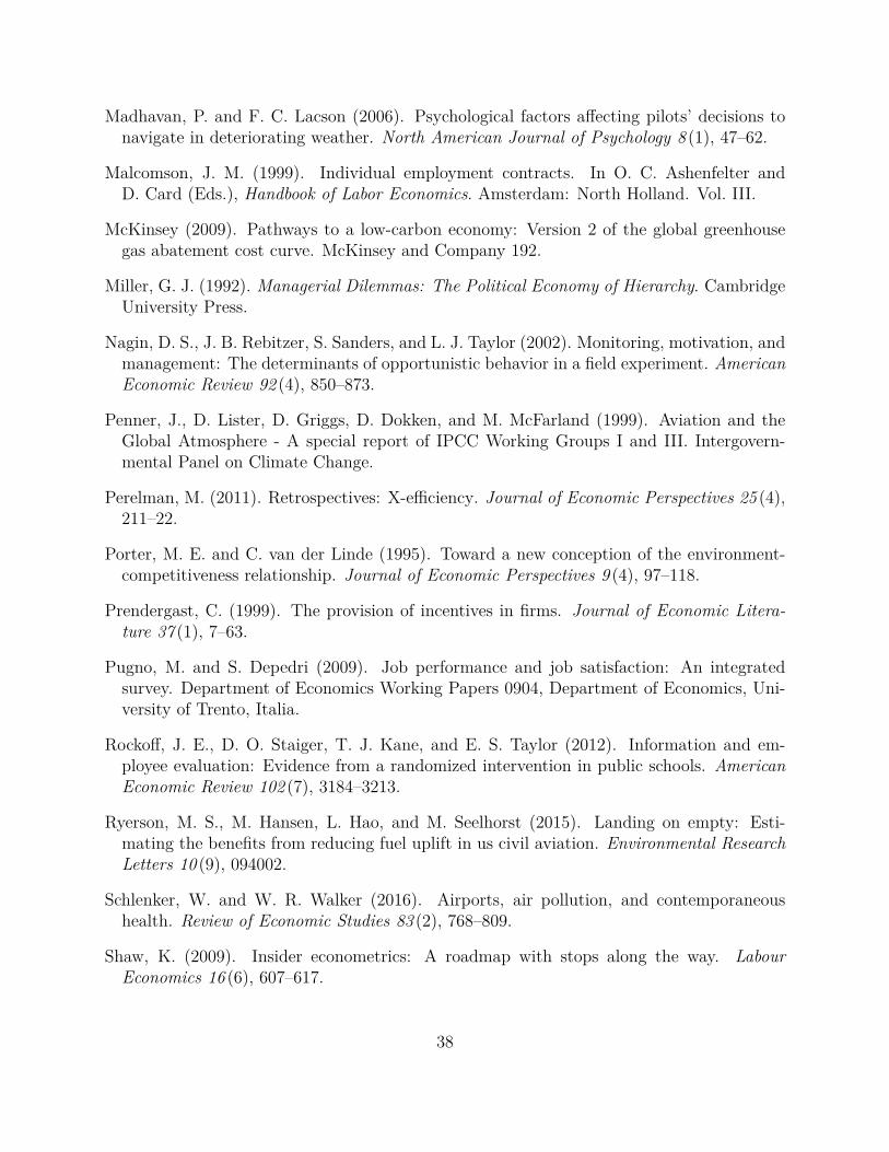
Madhavan, P. and F. C. Lacson (2006). Psychological factors affecting pilots’ decisions tonavigate in deteriorating weather. North American Journal of Psychology 8 (1), 47–62.

Malcomson, J. M. (1999). Individual employment contracts. In O. C. Ashenfelter andD. Card (Eds.), Handbook of Labor Economics. Amsterdam: North Holland. Vol. III.

McKinsey (2009). Pathways to a low-carbon economy: Version 2 of the global greenhousegas abatement cost curve. McKinsey and Company 192.

Miller, G. J. (1992). Managerial Dilemmas: The Political Economy of Hierarchy. CambridgeUniversity Press.

Nagin, D. S., J. B. Rebitzer, S. Sanders, and L. J. Taylor (2002). Monitoring, motivation, andmanagement: The determinants of opportunistic behavior in a field experiment. AmericanEconomic Review 92 (4), 850–873.

Penner, J., D. Lister, D. Griggs, D. Dokken, and M. McFarland (1999). Aviation and theGlobal Atmosphere - A special report of IPCC Working Groups I and III. Intergovern-mental Panel on Climate Change.

Perelman, M. (2011). Retrospectives: X-efficiency. Journal of Economic Perspectives 25 (4),211–22.

Porter, M. E. and C. van der Linde (1995). Toward a new conception of the environment-competitiveness relationship. Journal of Economic Perspectives 9 (4), 97–118.

Prendergast, C. (1999). The provision of incentives in firms. Journal of Economic Litera-ture 37 (1), 7–63.

Pugno, M. and S. Depedri (2009). Job performance and job satisfaction: An integratedsurvey. Department of Economics Working Papers 0904, Department of Economics, Uni-versity of Trento, Italia.

Rockoff, J. E., D. O. Staiger, T. J. Kane, and E. S. Taylor (2012). Information and em-ployee evaluation: Evidence from a randomized intervention in public schools. AmericanEconomic Review 102 (7), 3184–3213.

Ryerson, M. S., M. Hansen, L. Hao, and M. Seelhorst (2015). Landing on empty: Esti-mating the benefits from reducing fuel uplift in us civil aviation. Environmental ResearchLetters 10 (9), 094002.

Schlenker, W. and W. R. Walker (2016). Airports, air pollution, and contemporaneoushealth. Review of Economic Studies 83 (2), 768–809.

Shaw, K. (2009). Insider econometrics: A roadmap with stops along the way. LabourEconomics 16 (6), 607–617.

38

Shearer, B. (2004). Piece rates, fixed wages and incentives: Evidence from a field experiment.Review of Economic Studies 71 (2), 513–534.

Singh, V. and S. Sharma (2015). Fuel consumption optimization in air transport: A review,classification, critique, simple meta-analysis, and future research implications. EuropeanTransport Research Review 7 (2), 1–24.

Smith, P. (2013). Cockpit confidential: Everything you need to know about air travel:Questions, answers, and reflections. Sourcebooks.

Stern, N. (2006). Stern Review of the Economics of Climate Change. Report, HM Treasury,London.

Stiglitz, J. E. (1975). Incentives, risk, and information: Notes towards a theory of hierarchy.The Bell Journal of Economics 6 (2), 552–579.

Tonin, M. and M. Vlassopoulos (2010). Disentangling the sources of pro-socially motivatedeffort: A field experiment. Journal of Public Economics 94 (11), 1086–1092.

Tonin, M. and M. Vlassopoulos (2014). Corporate philanthropy and productivity: Evidencefrom an online real effort experiment. Management Science 61 (8), 1795–1811.

U.S. Enviromental Protection Agency (2015). Inventory of u.s. greenhouse gas emissions andsinks: 1990-2013. http://www3.epa.gov/climatechange/Downloads/ghgemissions/US-GHG-Inventory-2015-Main-Text.pdf. Accessed: July 15, 2015.

Walmsley, S. and A. Gilbey (2016). Cognitive biases in visual pilots’ weather-related decisionmaking. Applied Cognitive Psychology, Forthcoming.

Wiggins, M. W., D. R. Hunter, D. O’Hare, and M. Martinussen (2012). Characteristics ofpilots who report deliberate versus inadvertent visual flight into instrument meteorologicalconditions. Safety Science 50 (3), 472–477.

39

5 Figures and Tables

Figure 1Global destinations of VAA

40

Figure 2aFuel Load, by time period

.25

.3.3

5.4

.45

.5.5

5.6

.65

Fuel

Loa

d as

Pro

porti

on o

f Flig

hts

Control Information Targets Prosocial

Before During After

Figure 2bEfficient Flight, by time period

.25

.3.3

5.4

.45

.5.5

5.6

.65

Effi

cien

t Flig

ht a

s P

ropo

rtion

of F

light

s

Control Information Targets Prosocial

Before During After

41

Figure 2cEfficient Taxi, by time period

.25

.3.3

5.4

.45

.5.5

5.6

.65

Taxi

as

Pro

porti

on o

f Flig

hts

Control Information Targets Prosocial

Before During After

Figure 3aFuel Load before and during the experiment

.3.4

.5.6

.7

Jan−13 Apr−13 Jul−13 Oct−13 Feb−14 Apr−14 Jul−14 Sep−14

Control Control Linear FitInformation Information Linear FitTargets Targets Linear FitProsocial Prosocial Linear Fit

42

Figure 3bEfficient Flight before and during the experiment

.3.4

.5.6

.7

Jan−13 Apr−13 Jul−13 Oct−13 Feb−14 Apr−14 Jul−14 Sep−14

Control Control Linear FitInformation Information Linear FitTargets Targets Linear FitProsocial Prosocial Linear Fit

Figure 3cEfficient Taxi before and during the experiment

.3.4

.5.6

.7

Jan−13 Apr−13 Jul−13 Oct−13 Feb−14 Apr−14 Jul−14 Sep−14

Control Control Linear FitInformation Information Linear FitTargets Targets Linear FitProsocial Prosocial Linear Fit

43

Figure 4aTreatment effects for Fuel Load during the experiment

-.06

-.03

0.0

3.0

6.0

9.1

2.1

5.1

8Tr

eatm

ent E

ffect

as

Pro

porti

on o

f Flig

hts

Feb Mar Apr May Jun Jul Aug Sep

Information Targets Prosocial

Figure 4bTreatment effects for Efficient Flight during the experiment

-.06

-.03

0.0

3.0

6.0

9.1

2.1

5.1

8Tr

eatm

ent E

ffect

as

Pro

porti

on o

f Flig

hts

Feb Mar Apr May Jun Jul Aug Sep

Information Targets Prosocial

44

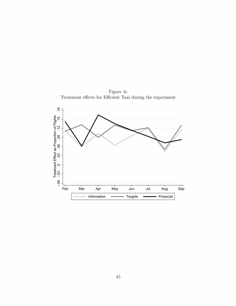
Figure 4cTreatment effects for Efficient Taxi during the experiment

-.06

-.03

0.0

3.0

6.0

9.1

2.1

5.1

8Tr

eatm

ent E

ffect

as

Pro

porti

on o

f Flig

hts

Feb Mar Apr May Jun Jul Aug Sep

Information Targets Prosocial

45

Figure 5aWithin-subject Changes in Control Group - Average Fuel Load Implementation from Beforeto During the Experiment

0

.2

.4

.6

.8

1

Fuel

Loa

d as

Pro

porti

on o

f Flig

hts

Captains (in ascending order of pre-experimental performance)

Notes: The data points in the graph represent the proportion of flights for which each captain in the ControlGroup implemented the Fuel Load behavior before the experiment (January 2013 - January 2014), in as-cending order of pre-experimental performance. The vertical arrows indicate represent the same proportionduring the experimental period (February 2014 - September 2014). An upward arrow indicates an improve-ment in implementation (as a proportion of total flights) of the behavior, while a downward arrow indicatesa decline in implementation.

46

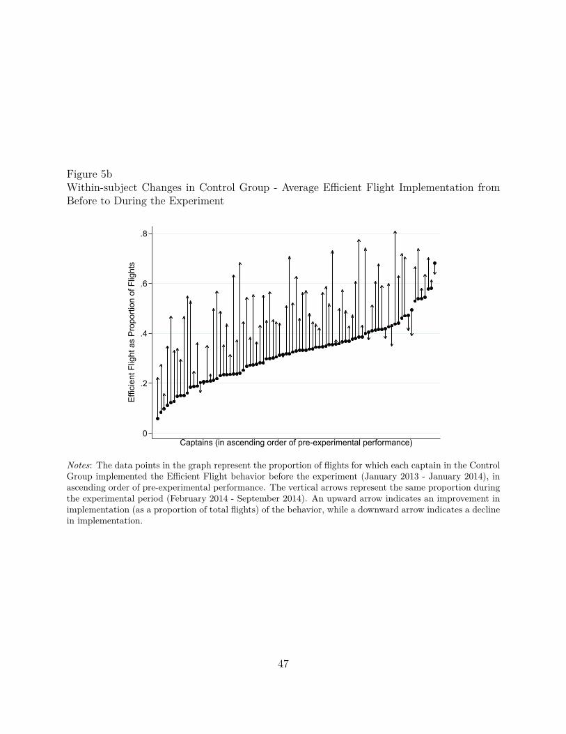
Figure 5bWithin-subject Changes in Control Group - Average Efficient Flight Implementation fromBefore to During the Experiment

0

.2

.4

.6

.8

Effi

cien

t Flig

ht a

s P

ropo

rtion

of F

light

s

Captains (in ascending order of pre-experimental performance)

Notes: The data points in the graph represent the proportion of flights for which each captain in the ControlGroup implemented the Efficient Flight behavior before the experiment (January 2013 - January 2014), inascending order of pre-experimental performance. The vertical arrows represent the same proportion duringthe experimental period (February 2014 - September 2014). An upward arrow indicates an improvement inimplementation (as a proportion of total flights) of the behavior, while a downward arrow indicates a declinein implementation.

47

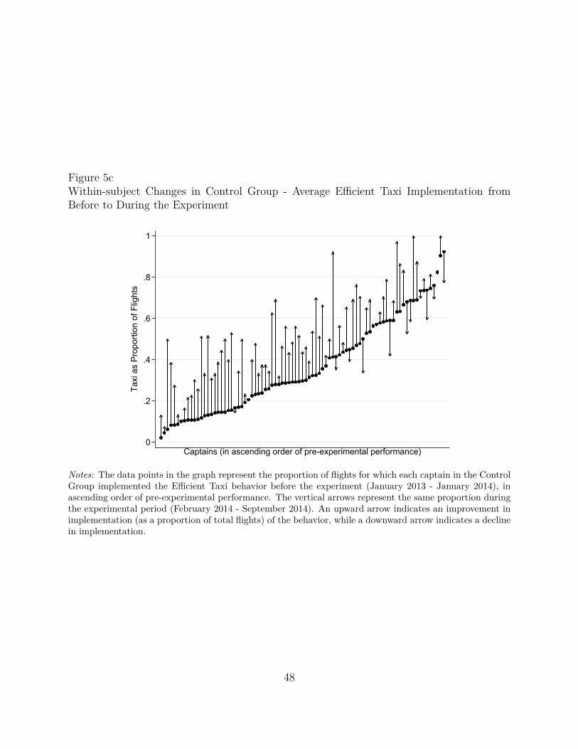
Figure 5cWithin-subject Changes in Control Group - Average Efficient Taxi Implementation fromBefore to During the Experiment

0

.2

.4

.6

.8

1

Taxi

as

Pro

porti

on o

f Flig

hts

Captains (in ascending order of pre-experimental performance)

Notes: The data points in the graph represent the proportion of flights for which each captain in the ControlGroup implemented the Efficient Taxi behavior before the experiment (January 2013 - January 2014), inascending order of pre-experimental performance. The vertical arrows represent the same proportion duringthe experimental period (February 2014 - September 2014). An upward arrow indicates an improvement inimplementation (as a proportion of total flights) of the behavior, while a downward arrow indicates a declinein implementation.

48

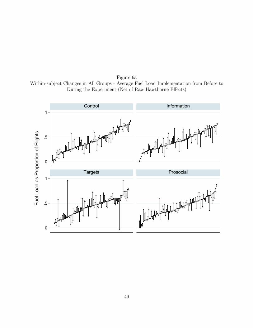
Figure 6aWithin-subject Changes in All Groups - Average Fuel Load Implementation from Before to

During the Experiment (Net of Raw Hawthorne Effects)

0

.5

1

0

.5

1

Control Information

Targets Prosocial

Fuel

Loa

d as

Pro

porti

on o

f Flig

hts

49

Figure 6bWithin-subject Changes in All Groups - Average Efficient Flight Implementation from

Before to During the Experiment (Net of Raw Hawthorne Effects)

-.5

0

.5

1

-.5

0

.5

1

Control Information

Targets Prosocial

Effi

cien

t Flig

ht a

s P

ropo

rtion

of F

light

s

50

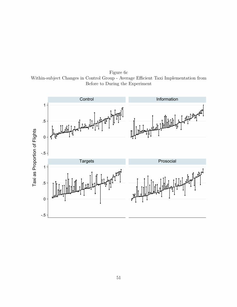
Figure 6cWithin-subject Changes in Control Group - Average Efficient Taxi Implementation from

Before to During the Experiment

-.5

0

.5

1

-.5

0

.5

1

Control Information

Targets Prosocial

Taxi

as

Pro

porti

on o

f Flig

hts

51

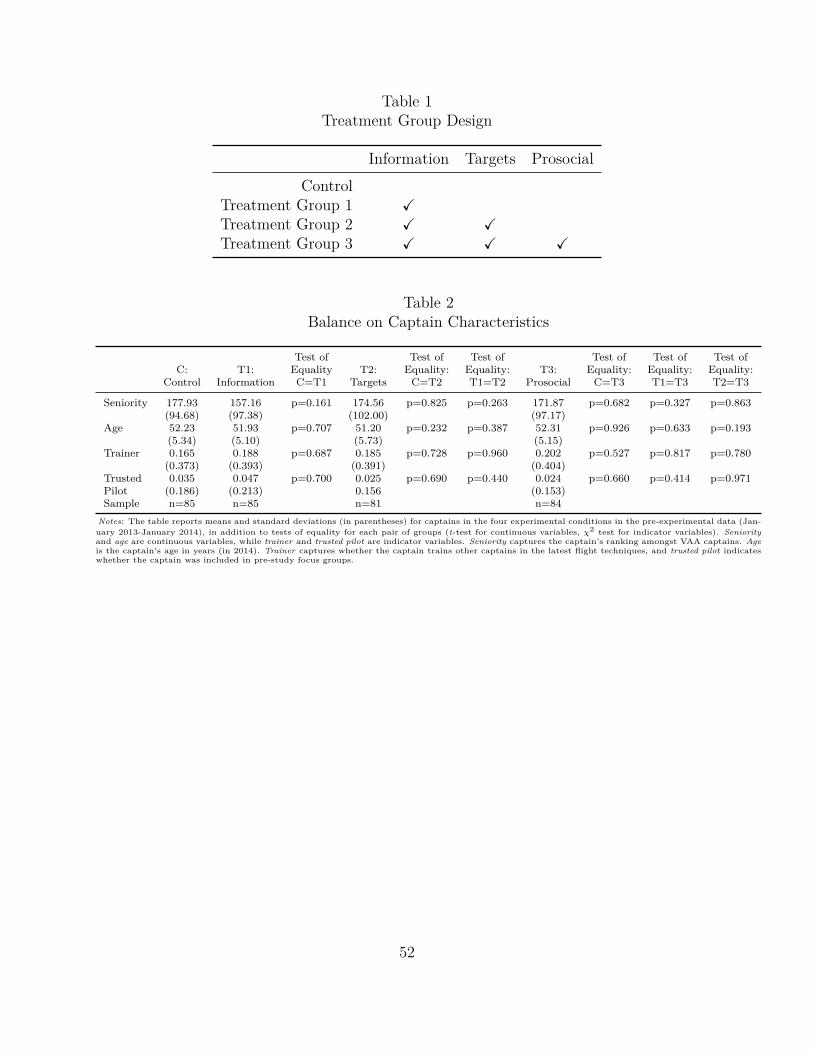
Table 1Treatment Group Design

Information Targets ProsocialControl

Treatment Group 1 XTreatment Group 2 X XTreatment Group 3 X X X

Table 2Balance on Captain Characteristics

Test of Test of Test of Test of Test of Test ofC: T1: Equality T2: Equality: Equality: T3: Equality: Equality: Equality:

Control Information C=T1 Targets C=T2 T1=T2 Prosocial C=T3 T1=T3 T2=T3

Seniority 177.93 157.16 p=0.161 174.56 p=0.825 p=0.263 171.87 p=0.682 p=0.327 p=0.863(94.68) (97.38) (102.00) (97.17)

Age 52.23 51.93 p=0.707 51.20 p=0.232 p=0.387 52.31 p=0.926 p=0.633 p=0.193(5.34) (5.10) (5.73) (5.15)

Trainer 0.165 0.188 p=0.687 0.185 p=0.728 p=0.960 0.202 p=0.527 p=0.817 p=0.780(0.373) (0.393) (0.391) (0.404)

Trusted 0.035 0.047 p=0.700 0.025 p=0.690 p=0.440 0.024 p=0.660 p=0.414 p=0.971Pilot (0.186) (0.213) 0.156 (0.153)Sample n=85 n=85 n=81 n=84

Notes: The table reports means and standard deviations (in parentheses) for captains in the four experimental conditions in the pre-experimental data (Jan-uary 2013-January 2014), in addition to tests of equality for each pair of groups (t-test for continuous variables, χ2 test for indicator variables). Seniorityand age are continuous variables, while trainer and trusted pilot are indicator variables. Seniority captures the captain’s ranking amongst VAA captains. Ageis the captain’s age in years (in 2014). Trainer captures whether the captain trains other captains in the latest flight techniques, and trusted pilot indicateswhether the captain was included in pre-study focus groups.

52

Table 3Balance on Flight Characteristics

Test of Test of Test of Test of Test of Test ofC: T1: Equality T2: Equality: Equality: T3: Equality: Equality: Equality:

Control Information C=T1 Targets C=T2 T1=T2 Prosocial C=T3 T1=T3 T2=T3

Plan Ramp 76,750 78,559 p=0.440 76,666 p=0.971 p=0.764 76,042 p=0.442 p=0.294 p=0.793(14,993) (15,467) (14,815) (15,587)

Engines 3.439 3.483 p=0.648 3.419 p=0.840 p=0.515 3.392 p=0.633 p=0.354 p=0.786(0.629) (0.615) (0.640) (0.658)

Flights/Month 5.182 5.150 p=0.877 5.305 p=0.571 p=0.465 5.261 p=0.706 p=0.586 p=0.837(1.372) (1.310) (1.406) (1.328)

Fuel Load 0.417 0.422 p=0.866 0.424 p=0.831 p=0.769 0.408 p=0.956 p=0.616 p=0.589(0.208) (0.175) (0.180) (0.185)

Eff Flight 0.322 0.322 p=0.979 0.327 p=0.778 p=0.835 0.326 p=0.789 p=0.849 p=0.942(0.124) (0.114) (0.130) (0.130)

Eff Taxi 0.365 0.359 p=0.874 0.367 p=0.947 p=0.460 0.339 p=0.821 p=0.561 p=0.418(0.230) (0.229) (0.222) (0.226)

Sample n=85 n=85 n=81 n=84Notes: The table reports means and standard deviations (in parentheses) for captains in the four experimental conditions in the pre-experimental data (January 2013-January 2014),in addition to tests of equality for each pair of groups (empht-test for continuous variables, χ2 test for indicator variables). Plan Ramp measures the amount of fuel anticipated for theentire flight (including taxi-out and taxi-in) and therefore acts as a proxy for distance flown. Engines is the average number of engines on aircraft flown. Flights/Month is the averagenumber of flights a captain flew in a given month in the thirteen months leading up to the study. Fuel Load, Eff Flight, and Eff Taxi represent the proportion of each captain’s flights onwhich each of the three fuel-efficient behaviors targeted by the study were met in the pre-experimental period.

53

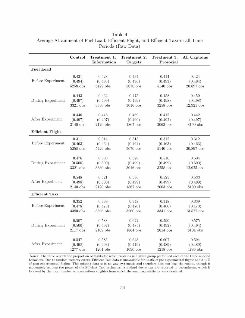
Table 4Average Attainment of Fuel Load, Efficient Flight, and Efficient Taxi-in all Time

Periods (Raw Data)

Control Treatment 1: Treatment 2: Treatment 3: All CaptainsInformation Targets Prosocial

Fuel Load

Before Experiment0.421 0.428 0.434 0.414 0.424(0.494) (0.495) (0.496) (0.493) (0.494)5258 obs 5429 obs 5070 obs 5140 obs 20,897 obs

During Experiment0.443 0.462 0.475 0.458 0.459(0.497) (0.499) (0.499) (0.498) (0.498)3321 obs 3330 obs 3016 obs 3258 obs 12,925 obs

After Experiment0.446 0.446 0.469 0.412 0.442(0.497) (0.497) (0.499) (0.492) (0.497)2140 obs 2120 obs 1867 obs 2063 obs 8190 obs

Efficient Flight

Before Experiment0.311 0.314 0.313 0.312 0.312(0.463) (0.464) (0.464) (0.463) (0.463)5258 obs 5429 obs 5070 obs 5140 obs 20,897 obs

During Experiment0.476 0.503 0.528 0.510 0.504(0.500) (0.500) (0.499) (0.499) (0.500)3321 obs 3330 obs 3016 obs 3258 obs 12,925 obs

After Experiment0.548 0.521 0.536 0.525 0.533(0.498) (0.500) (0.499) (0.499) (0.499)2140 obs 2120 obs 1867 obs 2063 obs 8190 obs

Efficient Taxi

Before Experiment0.352 0.339 0.348 0.318 0.339(0.478) (0.473) (0.476) (0.466) (0.473)3380 obs 3596 obs 3260 obs 3341 obs 13,577 obs

During Experiment0.507 0.588 0.622 0.590 0.575(0.500) (0.492) (0.485) (0.492) (0.494)2117 obs 2109 obs 1864 obs 2014 obs 8104 obs

After Experiment0.547 0.585 0.643 0.607 0.594(0.498) (0.493) (0.479) (0.489) (0.489)1277 obs 1201 obs 1090 obs 1218 obs 4786 obs

Notes: The table reports the proportion of flights for which captains in a given group performed each of the three selectedbehaviors. Due to random memory errors, Efficient Taxi data is unavailable for 35.0% of pre-experimental flights and 37.2%of post-experimental flights. This missing data is in no way systematic and therefore does not bias the results, though itmoderately reduces the power of the Efficient Taxi estimates. Standard deviations are reported in parentheses, which isfollowed by the total number of observations (flights) from which the summary statistics are calculated.

54

Table 5Treatment Effect Identification using Difference-in-Difference Regression

(1) (2) (3) (4) (5) (6)Fuel Load Eff Flight Eff Taxi Fuel Load Eff Flight Eff Taxi

Expt 0.018 0.144*** 0.125*** 0.018 0.144*** 0.125***(0.012) (0.012) (0.017) (0.011) (0.011) (0.013)

Expt · Information 0.007 0.017 0.081*** 0.007 0.017 0.081***(0.017) (0.016) (0.025) (0.015) (0.014) (0.017)

Expt · Targets 0.021 0.037** 0.097*** 0.021 0.037** 0.097***(0.018) (0.018) (0.026) (0.015) (0.015) (0.018)

Expt · Prosocial 0.025 0.047*** 0.089*** 0.025* 0.047*** 0.089***(0.016) (0.017) (0.027) (0.015) (0.014) (0.018)

Observations 33,822 33,822 21,681 33,822 33,822 21,681N 335 335 335 335 335 335Controls Yes Yes Yes Yes Yes YesStandard Errors:Clustered Yes Yes YesNewey-West Yes Yes Yes

Notes: The table shows the results of two difference-in-difference regression specifications with captain fixed effect comparingpre-experiment behavior (January 2013-January 2014) to behavior during the experiment (February 2014-September 2014). Thedependent variables in the regressions are dummies capturing whether the fuel-efficient behavior was performed, and since pre-dicted values are not constrained between 0 and 1, we do not report a constant and instead focus on treatment effects. As such,the coefficients indicate the increase in the proportion of flights beyond the control group for which the behavior of interest wassuccessfully performed. We provide conventional robust standard errors clustered at the captain level and Newey-West standarderrors (lag=1). Total flight observations are provided. Controls include weather on departure and arrival, number of engines on theaircraft, aircraft type, ports of departure and arrival, aircraft maintenance, captains’ contracted hours, and whether the captainhas completed training. ∗∗∗p < 0.01 ∗∗p < 0.05 ∗p < 0.10

55

Table 6Persistence: Treatment Effect Identification using Difference-in-Difference Regression

Comparing Behavior Before Experiment to After Experiment

(1) (2) (3) (4) (5) (6)Fuel Load Eff Flight Eff Taxi Fuel Load Eff Flight Eff Taxi

Post 0.049** 0.215*** 0.152*** 0.049** 0.215*** 0.152***(0.024) (0.021) (0.035) (0.021) (0.020) (0.029)

Post · Information -0.007 -0.021 0.040 -0.007 -0.021 0.040*(0.020) (0.021) (0.030) (0.017) (0.016) (0.021)

Post · Targets 0.018 0.003 0.057** 0.018 0.003 0.057***(0.020) (0.022) (0.026) (0.018) (0.017) (0.022)

Post · Prosocial -0.020 0.002 0.058** -0.020 0.002 0.058***(0.021) (0.020) (0.025) (0.017) (0.016) (0.021)

Observations 29,087 29,087 18,363 29,087 29,087 18,363N 335 335 335 335 335 335Controls Yes Yes Yes Yes Yes Yes

Standard Errors:Clustered Yes Yes YesNewey-West Yes Yes Yes

Notes: The table shows the results of two difference-in-difference regression specifications with captain fixed effect com-paring pre-experiment behavior (January 2013-January 2014) to post-experiment behavior (“Post”: October 2014-March2015). The dependent variables in the regressions are dummies capturing whether the fuel-efficient behavior was performed,and since predicted values are not constrained between 0 and 1, we do not report a constant and instead focus on treat-ment effects. As such, the coefficients indicate the increase in the proportion of flights beyond the control group for whichthe behavior of interest was successfully performed. We provide conventional robust standard errors clustered at the cap-tain level and Newey-West standard errors (lag=1). Total flight observations are provided. Controls include weather ondeparture and arrival, number of engines on the aircraft, aircraft type, ports of departure and arrival, aircraft maintenance,captains’ contracted hours, and whether the captain has completed training. ∗∗∗p < 0.01 ∗∗p < 0.05 ∗p < 0.10

56

Table 7Data-Supported Estimates of Overall Fuel Savings (in

tons)

(1) (2)Fuel Savings Fuel Savings

Control 755.32*** 1,647.79***(166.38) (207.54)

Information 1,230.28*** 2,152.39***(169.70) (215.51)

Targets 1,171.59*** 1,994.37***(158.41) (194.10)

Prosocial 1,089.35*** 1,973.99***(166.88) (206.15)

Total Fuel Savings 4,246.54 7,768.54Linear Time Trend No Yes

Notes: The table presents estimates of total fuel savings by treatment group.Savings are based on regression coefficients from a difference-in-differencespecification with captain fixed effects comparing pre-experiment behavior(January 2013-January 2014) to behavior during the experiment (February2014-September 2014). The dependent variable is the deviation between ac-tual fuel used and predicted fuel use in the flight plan. We calculate fuel sav-ings with an intent-to-treat approach where the regression coefficient of eachgroup (i.e., the group’s average treatment effect) and the average Hawthorneeffect (i.e., the coefficient of the Experimental-period indicator) are multipliedby the number of flights in each group (3321, 3330, 3016, and 3258 respec-tively). In other words, we assume that the Hawthorne effect is proportionalto the number of flights. The per-flight fuel savings estimates for the control,information, targets, and prosocial incentives groups—controlling for a lin-ear time trend—are (respectively): 496.17 (p<0.01), 150.19 (p<0.05), 165.09(p<0.05), and 109.72 (p=0.10). Standard error calculations are based onNewey-West standard errors (lag=1). Controls include weather on departureand arrival, number of engines on the aircraft, aircraft type, ports of departureand arrival, aircraft maintenance, captains’ contracted hours, and whetherthe captain has completed training. ∗∗∗p < 0.01 ∗∗p < 0.05 ∗p < 0.10

57

Table 8Engineering Estimates of Fuel Savings

# Flights Fuel Load Efficient Flight Efficient Taxi Fuel Load Efficient Flight Efficient Taxi

Control 3321 1.8% increase 14.4% increase 12.5% increase 3.3% increase 13.2% increase 3.8% increase(59.8 flights) (478.2 flights) (415.1 flights) (109.6 flights) (438.4 flights) (126.2 flights)

Information 3330 2.5% increase 16.1% increase 20.6% increase 4.0% increase 14.9% increase 11.7% increase(83.3 flights) (536.1 flights) (686.0 flights) (133.2 flights) (496.2 flights) (389.6 flights)

Targets 3016 3.9% increase 18.1% increase 22.2% increase 5.5% increase 16.9% increase 13.4% increase(117.6 flights) (545.9 flights) (669.6 flights) (165.9 flights) (509.7 flights) (404.1 flights)

Prosocial 3258 4.3% increase 19.1% increase 21.4% increase 5.8% increase 17.9% increase 12.6% increase(140.1 flights) (622.3 flights) (697.2 flights) (189.0 flights) (583.2 flights) (410.5 flights)

VAA ProjectedSavings/Flight 250 kg 500 kg 72 kg 250 kg 500 kg 72 kg

Fuel Savings fromBehavior Change 100.19 tons 1,091.26 tons 177.69 tons 149.41 tons 1,013.71 tons 95.79 tons

Total Fuel Savings 1,369.14 tons 1,258.92 tons

Linear Time Trend No No No Yes Yes Yes58

Table 9Costs of Fuel Usage

Purchase Cost CO2 Cost Total CostFuel (1 ton) $786 $116.55 $902.55

Notes: The table shows the cost of fuel usage. We use global jet fuel prices inFebruary 2014 (first month of treatment), estimates of the social cost of car-bon of $37/ton, and the September 30, 2014 exchange rate ($1 = £0.6167) forall calculations. One ton of fuel emits about 3.15 tons of CO2. These valuesare used for calculations of savings in the text.

59

A Appendix I: Additional Tables

Table A1Test of a Unit Root of Pre-Experiment Behaviors

Fuel Load Eff Flight Eff Taxi

Z(t) -3.765*** -2.562* -6.431***(0.003) (0.010) (0.000)

Observations (weeks) 51 51 51Notes: The table shows the Dickey-Fuller (DF) test for a unit root for the51 weeks before the experiment started, collapsing all the groups into one foreach behavior. The null of the DF test is a unit root, and the rejection ofthe null is that the data follows a random walk. Z(t) is the DF test statistic.∗∗∗p < 0.01 ∗∗p < 0.05 ∗p < 0.10

60

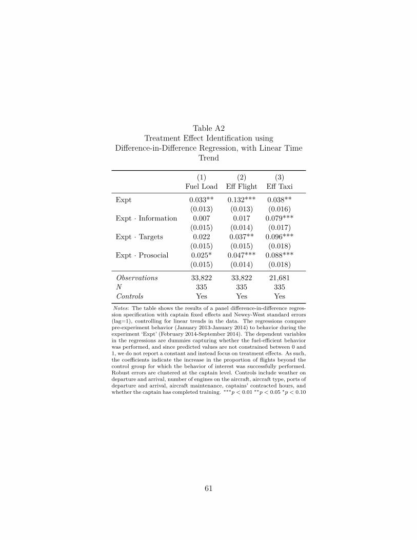
Table A2Treatment Effect Identification using

Difference-in-Difference Regression, with Linear TimeTrend

(1) (2) (3)Fuel Load Eff Flight Eff Taxi

Expt 0.033** 0.132*** 0.038**(0.013) (0.013) (0.016)

Expt · Information 0.007 0.017 0.079***(0.015) (0.014) (0.017)

Expt · Targets 0.022 0.037** 0.096***(0.015) (0.015) (0.018)

Expt · Prosocial 0.025* 0.047*** 0.088***(0.015) (0.014) (0.018)

Observations 33,822 33,822 21,681N 335 335 335Controls Yes Yes Yes

Notes: The table shows the results of a panel difference-in-difference regres-sion specification with captain fixed effects and Newey-West standard errors(lag=1), controlling for linear trends in the data. The regressions comparepre-experiment behavior (January 2013-January 2014) to behavior during theexperiment ‘Expt’ (February 2014-September 2014). The dependent variablesin the regressions are dummies capturing whether the fuel-efficient behaviorwas performed, and since predicted values are not constrained between 0 and1, we do not report a constant and instead focus on treatment effects. As such,the coefficients indicate the increase in the proportion of flights beyond thecontrol group for which the behavior of interest was successfully performed.Robust errors are clustered at the captain level. Controls include weather ondeparture and arrival, number of engines on the aircraft, aircraft type, ports ofdeparture and arrival, aircraft maintenance, captains’ contracted hours, andwhether the captain has completed training. ∗∗∗p < 0.01 ∗∗p < 0.05 ∗p < 0.10

61

Table A3Treatment Effect Identification using Difference-in-Difference Regression with

Quadruplet Controls

(1) (2) (3) (4) (5) (6)Fuel Load Eff Flight Eff Taxi Fuel Load Eff Flight Eff Taxi

Expt 0.022 0.146*** 0.140*** 0.022** 0.146*** 0.140***(0.015) (0.013) (0.016) (0.010) (0.009) (0.011)

Expt · Information 0.017 0.023 0.065*** 0.017 0.023** 0.065***(0.020) (0.016) (0.022) (0.012) (0.011) (0.014)

Expt · Targets 0.022 0.041** 0.092*** 0.022* 0.041*** 0.092***(0.020) (0.016) (0.022) (0.012) (0.012) (0.015)

Expt · Prosocial 0.011 0.042*** 0.078*** 0.011 0.042*** 0.078***(0.019) (0.016) (0.023) (0.012) (0.011) (0.014)

Observations 33,822 33,822 21,681 33,822 33,822 21,681N 335 335 335 335 335 335Controls Yes Yes Yes Yes Yes Yes

Standard Errors:Clustered Yes Yes YesNewey-West Yes Yes Yes

Notes: The table shows the results of two difference-in-difference regression specifications with quadruplet fixed effects com-paring pre-experiment behavior (January 2013-January 2014) to behavior during the experiment (February 2014-September2014). The dependent variables in the regressions are dummies capturing whether the fuel-efficient behavior was performed,and since predicted values are not constrained between 0 and 1, we do not report a constant and instead focus on treatmenteffects. As such, the coefficients indicate the increase in the proportion of flights beyond the control group for which the be-havior of interest was successfully performed. We provide conventional robust standard errors clustered at the captain leveland Newey-West standard errors (lag=1). Total flight observations are provided. Controls include weather on departureand arrival, number of engines on the aircraft, aircraft type, ports of departure and arrival, aircraft maintenance, captains’contracted hours, and whether the captain has completed training. ∗∗∗p < 0.01 ∗∗p < 0.05 ∗p < 0.10

62

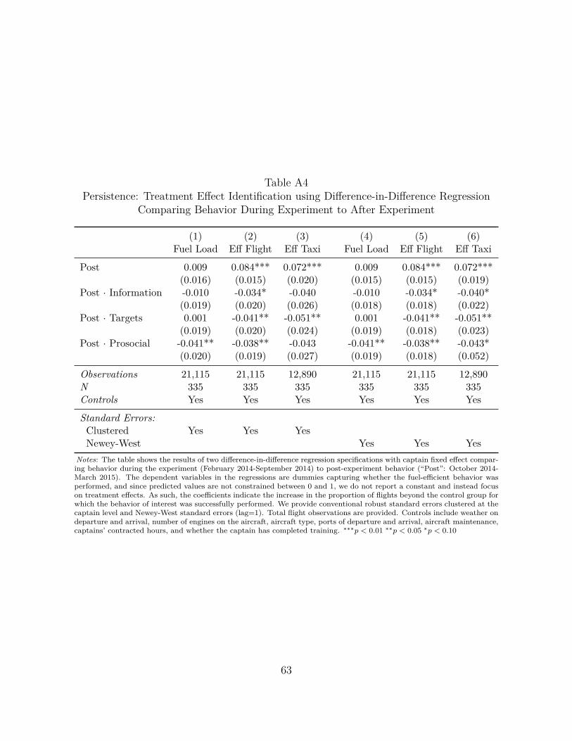
Table A4Persistence: Treatment Effect Identification using Difference-in-Difference Regression

Comparing Behavior During Experiment to After Experiment

(1) (2) (3) (4) (5) (6)Fuel Load Eff Flight Eff Taxi Fuel Load Eff Flight Eff Taxi

Post 0.009 0.084*** 0.072*** 0.009 0.084*** 0.072***(0.016) (0.015) (0.020) (0.015) (0.015) (0.019)

Post · Information -0.010 -0.034* -0.040 -0.010 -0.034* -0.040*(0.019) (0.020) (0.026) (0.018) (0.018) (0.022)

Post · Targets 0.001 -0.041** -0.051** 0.001 -0.041** -0.051**(0.019) (0.020) (0.024) (0.019) (0.018) (0.023)

Post · Prosocial -0.041** -0.038** -0.043 -0.041** -0.038** -0.043*(0.020) (0.019) (0.027) (0.019) (0.018) (0.052)

Observations 21,115 21,115 12,890 21,115 21,115 12,890N 335 335 335 335 335 335Controls Yes Yes Yes Yes Yes Yes

Standard Errors:Clustered Yes Yes YesNewey-West Yes Yes Yes

Notes: The table shows the results of two difference-in-difference regression specifications with captain fixed effect compar-ing behavior during the experiment (February 2014-September 2014) to post-experiment behavior (“Post”: October 2014-March 2015). The dependent variables in the regressions are dummies capturing whether the fuel-efficient behavior wasperformed, and since predicted values are not constrained between 0 and 1, we do not report a constant and instead focuson treatment effects. As such, the coefficients indicate the increase in the proportion of flights beyond the control group forwhich the behavior of interest was successfully performed. We provide conventional robust standard errors clustered at thecaptain level and Newey-West standard errors (lag=1). Total flight observations are provided. Controls include weather ondeparture and arrival, number of engines on the aircraft, aircraft type, ports of departure and arrival, aircraft maintenance,captains’ contracted hours, and whether the captain has completed training. ∗∗∗p < 0.01 ∗∗p < 0.05 ∗p < 0.10

63

Table A5Difference-in-Difference

Regression of Flight Time

Flight Time

Expt 1.788***(0.522)

Expt · Information 0.011(0.687)

Expt · Targets 0.114(0.733)

Expt · Prosocial -1.586*(0.849)

Observations 33,822N 335Controls Yes

Notes: The dependent variable in this regres-sion is flight time in minutes. Captain fixedeffects are included and Newey-West standarderrors (lag = 1) are reported below estimatesin parentheses. Total flight observations areprovided. Controls include weather on depar-ture and arrival, number of engines on theaircraft, aircraft type, ports of departure andarrival, aircraft maintenance, captains’ con-tracted hours, and whether the captain hascompleted training. ∗∗∗p < 0.01 ∗∗p <0.05 ∗p < 0.10

64

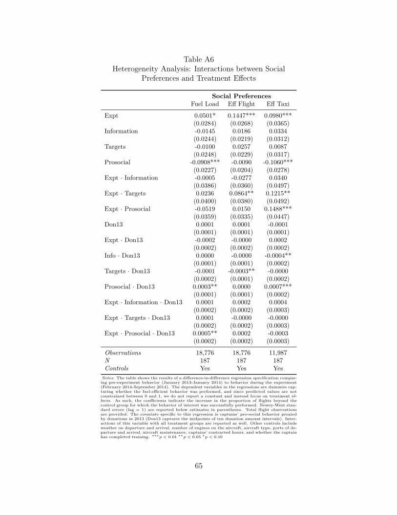
Table A6Heterogeneity Analysis: Interactions between Social

Preferences and Treatment Effects

Social PreferencesFuel Load Eff Flight Eff Taxi

Expt 0.0501* 0.1447*** 0.0980***(0.0284) (0.0268) (0.0365)

Information -0.0145 0.0186 0.0334(0.0244) (0.0219) (0.0312)

Targets -0.0100 0.0257 0.0087(0.0248) (0.0229) (0.0317)

Prosocial -0.0908*** -0.0090 -0.1060***(0.0227) (0.0204) (0.0278)

Expt · Information -0.0005 -0.0277 0.0340(0.0386) (0.0360) (0.0497)

Expt · Targets 0.0236 0.0864** 0.1215**(0.0400) (0.0380) (0.0492)

Expt · Prosocial -0.0519 0.0150 0.1488***(0.0359) (0.0335) (0.0447)

Don13 0.0001 0.0001 -0.0001(0.0001) (0.0001) (0.0001)

Expt · Don13 -0.0002 -0.0000 0.0002(0.0002) (0.0002) (0.0002)

Info · Don13 0.0000 -0.0000 -0.0004**(0.0001) (0.0001) (0.0002)

Targets · Don13 -0.0001 -0.0003** -0.0000(0.0002) (0.0001) (0.0002)

Prosocial · Don13 0.0003** 0.0000 0.0007***(0.0001) (0.0001) (0.0002)

Expt · Information · Don13 0.0001 0.0002 0.0004(0.0002) (0.0002) (0.0003)

Expt · Targets · Don13 0.0001 -0.0000 -0.0000(0.0002) (0.0002) (0.0003)

Expt · Prosocial · Don13 0.0005** 0.0002 -0.0003(0.0002) (0.0002) (0.0003)

Observations 18,776 18,776 11,987N 187 187 187Controls Yes Yes Yes

Notes: The table shows the results of a difference-in-difference regression specification compar-ing pre-experiment behavior (January 2013-January 2014) to behavior during the experiment(February 2014-September 2014). The dependent variables in the regressions are dummies cap-turing whether the fuel-efficient behavior was performed, and since predicted values are notconstrained between 0 and 1, we do not report a constant and instead focus on treatment ef-fects. As such, the coefficients indicate the increase in the proportion of flights beyond thecontrol group for which the behavior of interest was successfully performed. Newey-West stan-dard errors (lag = 1) are reported below estimates in parentheses. Total flight observationsare provided. The covariate specific to this regression is captains’ pro-social behavior proxiedby donations in 2013 (Don13 captures the midpoints of ten donation amount intervals). Inter-actions of this variable with all treatment groups are reported as well. Other controls includeweather on departure and arrival, number of engines on the aircraft, aircraft type, ports of de-parture and arrival, aircraft maintenance, captains’ contracted hours, and whether the captainhas completed training. ∗∗∗p < 0.01 ∗∗p < 0.05 ∗p < 0.10

65

Table A7Job Satisfaction and Treatment

Group

Job SatisfactionInformation 0.212

(0.224)Targets 0.0242

(0.249)Prosocial 0.365

(0.224)Constant 5.58***

(0.174)N 202

Notes: The dependent variable in this re-gression is a 7-point scale of job satisfac-tion, where self-reported job satisfaction in-creases in the scale. Robust standard errorsare reported below estimates in parentheses.∗∗∗p < 0.01 ∗∗p < 0.05 ∗p < 0.10

66

Table A8Job Satisfaction and Job Performance

Groups: Control and Information Targets and ProsocialJob Satisfaction Job Satisfaction

Fuel Load Targets Met 0.093 - 0.065 -(0.062) (0.060)

Eff Flight Targets Met -0.074 - -0.017 -(0.056) (0.054)Eff Taxi Targets Met 0.025 - 0.120** -(0.043) (0.054)

Overall Targets Met - 0.006 - 0.058*(0.028) (0.031)

Constant 5.691*** 5.632*** 5.341*** 5.326***(0.291) (0.300) (0.358) (0.358)

Observations 103 99N 103 99Controls No No

Notes: The dependent variable in these regressions is a 7-point scale of job satisfaction, where self-reportedjob satisfaction increases in the scale. Robust standard errors are reported below estimates in parentheses.The independent variables indicate the number of targets met per behavior and overall over the course of thestudy. ∗∗∗p < 0.01 ∗∗p < 0.05 ∗p < 0.10

67

B Appendix II: Theoretical Model

B.1 Model Setup

We consider a static choice problem that determines a captain’s chosen effort on the job in acertain period. In our model, we assume that captains, who have vast flying experience, areat an equilibrium fuel usage with respect to their wealth, experience, effort, and concernsfor safety, the environment, and company profitability.47

A captain faces the following additively separable utility function:

U(w, s, e, f, g) = u(w, e, g) + a · v(d(e) · g, g0, G−i) + y(s, e, f)− c(e)− s(e) (1)

where u(·) is utility from monetary wealth, v(·) is utility from giving to charity (pro-socialbehavior), y(·) is utility from job performance, c(·) is disutility from exerting effort, ands(·) describes disutility from social pressure. Effort is chosen for all three flight tasks, j,i.e., Fuel Load, Efficient Flight, and Efficient Taxi. Captains observe their effort perfectly.They also receive a noisy signal of fuel usage fit + εit = fit. fit describes the estimatedfuel usage by captain i for flight t which depends on the chosen effort for the fuel-efficientactivities. fit is actual fuel use, observed ex post by the airline, which also includes a randomcomponent.48 Furthermore, each captain has an ideal fuel usage fI , which is based on herown experience and environmental and firm profit preferences. By revealed preference theequilibrium pre-study fuel usage is fI = f .

Experimental treatments in this study alter three model parameters. First, receivinginformation on fuel use, i = 1(information), removes the noisiness of the fuel signal, i.e.,fit + (1− i)εit = fit. Second, provision of a target, r = 1(target), changes the captain’s idealfuel usage, fI , because the employer exogenously imposes a target level. Then, fI = fT ifr = 1 where fT reflects the signaled optimal usage from the point of view of the airline.Third, in the pro-social behavior treatment a donation, g, is made by the airline in the nameof the captain. This donation is conditional on meeting the target which has a probability

47In a survey, captains in the study expressed a concern over fuel usage and fuel cost, both for environ-mental reasons and company profitability. To become an airline captain requires many years of training andexperience within an airline; if a captain loses her job with one airline and seeks employment in another, sheloses her prior seniority and must work for many years to reinstate it. Thus, for the sake of their own jobsecurity, captains care about minimizing fuel costs.

48Due to the vast experience of captains, we assume E(εit) = 0, i.e., captains predict fuel usage correctly,on average.

68

of d(e) in this treatment.49 In all other treatments, reaching particular fuel use levels doesnot lead to donations, i.e., d(e) = 0. Parameters and elements of the utility function areexplained in more detail below.

(Dis)utility from social pressure. In the spirit of DellaVigna et al. (2012, “DLM” here-after) and Bénabou and Tirole (2006), we assume that captains are either affected by socialpressure due to their actions being observed or exhibit some sort of social signaling in whichthey want to appear to be good employees. In this framework, captains are aware of an op-timal, social effort level, esocial. Because exerting effort is costly to the captain and becauseher actions are imperfectly observed with probability πobserved < 1, generally e > esocial.50

In this study, captains in both the control group and treatment group are made aware thattheir actions are monitored and data on their effort are used for an internal and academicstudy. Consequently, we expect the probability of detection of deviations from the socialeffort level to increase for all participants in the study relative to the pre-study period, i.e.,πobservedstudy > πobservedpre . We parameterize social pressure as follows:

s(e) = [πobserved · (esocial − e) + (1− πobserved) · 0] · 1(e < esocial)

Social pressure decreases utility if the chosen effort level is below the socially optimaleffort level of the captain. This disutility is increasing in the distance from the optimaleffort level and in the probability of these actions being observed by the airline. The secondterm is an indicator function implying that unobserved deviations do not lead to disutility..For agents that exert more effort than esocial, s(e) simply drops out of their utility function.Consequently, captains can directly impact the level of disutility by exerting more (costly)effort.

Note that s(e) enters the utility of every captain below the social effort level, regardless oftreatment assignment. If social pressure is important, even control captains should respondto this increased cost of low effort.51 Because s(e) is orthogonal to treatment, we omit it in

49Captains can directly influence the probability with their effort. That is, captains can be certain thatthey do not meet a target if they put in little effort, and they can be certain that they have achieved thetarget if they put in sufficient effort.

50It is plausible to argue that effort is perfectly observed in the aviation industry with modern technology.However, captains might not expect these data to be analyzed on a regular basis.

51Alternatively, we could interpret esocial as a level of effort induced by the researcher, leading toexperimenter-demand effects. Put differently, captains in the study could think they are expected to in-crease effort and not doing so imposes utility costs on them.

69

the following discussion and in the derivation of comparative statics.52

Utility from wealth. Similar to DLM, for wealth w, charitable giving from the airline gfor meeting the target (if applicable), and other charitable giving g0, u is defined as follows:

u(w, e, g) = u(w − g0(d(e) · g) + a · d(e) · g)

where a =

0 if a < 0

a if 0 ≤ a ≤ 1

1 if a > 1

Private consumption is an individual’s wealth minus the amount given to charity fromthat person’s wealth (i.e., not from this study). However, to ensure that u is continuouslydifferentiable, we need to account for the effect of charitable donations resulting from ourtreatments on utility from private consumption. To capture this effect, we multiply theindividual’s expected donation, d(e)·g, by a function of a—a parameter capturing preferencesfor giving—which we call a. As in DLM, the parameter a is non-negative in the case of pureor impure altruism and negative in the case of spite53, and a is simply a truncated at 0 and1.

The reasons for creating such boundaries on the term capturing preferences for giving aretwofold. First, an individual with spiteful preferences (a < 0) does not get less utility fromprivate consumption when she donates to charity than when she does not donate to charity;therefore, a is censored from below at 0. Second, an individual with pure or impure altruisticpreferences will get additional utility from her private consumption by giving to charitythrough our treatment because it corresponds to an outward shift in the budget constraintin the dimension of giving to the chosen charity. However, a is censored from above at 1because an individual will experience weakly more utility from increases in w than fromgiving to the chosen charity (i.e., ∂u

∂w≥ ∂u

∂g). This relation holds since increases in w shift the

budget constraint outward in all dimensions—including the charitable giving dimension—so52Social pressure is additively separable from other utility elements in a linear model. Consequently, it

does not affect the sign of comparative statics derived below and, if interactions are present, only attenuatestreatment effect estimates.

53As defined in Andreoni (1989, 1990), pure and impure altruism capture two possible motivations forgiving. The first stems from a preference solely for provision of the public good, so that an individual’sdonations are entirely crowded out by donations from other sources. Impure altruism, on the other hand,refers to the phenomenon whereby individuals receive direct utility from the act of giving itself, i.e., through“warm glow”. Spite, as defined in DLM, exists when an individual gets disutility from donating to the charity.

70

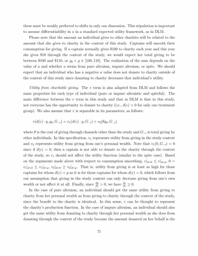
these must be weakly preferred to shifts in only one dimension. This stipulation is importantto assume differentiability in u in a standard expected utility framework, as in DLM.

Please note that the amount an individual gives to other charities will be related to theamount that she gives to charity in the context of this study. Captains will smooth theirconsumption for giving. If a captain normally gives $100 to charity each year and this yearshe gives $10 through the context of the study, we would expect her total giving to bebetween $100 and $110, or g0 + g ∈ [100, 110]. The realization of the sum depends on thevalue of a and whether a stems from pure altruism, impure altruism, or spite. We shouldexpect that an individual who has a negative a value does not donate to charity outside ofthe context of this study since donating to charity decreases that individual’s utility.

Utility from charitable giving. The v term is also adapted from DLM and follows thesame properties for each type of individual (pure or impure altruistic and spiteful). Themain difference between the v term in this study and that in DLM is that in this study,not everyone has the opportunity to donate to charity (i.e., d(e) > 0 for only one treatmentgroup). We also assume that v is separable in its parameters, as follows:

v(d(e) · g, g0, G−i) = v1(d(e) · g,G−i) + v2(θg0, G−i)

where θ is the cost of giving through channels other than the study and G−i is total giving byother individuals. In this specification, v1 represents utility from giving in the study contextand v2 represents utility from giving from one’s personal wealth. Note that v1(0, G−i) = 0since if d(e) = 0, then a captain is not able to donate to the charity through the contextof the study, so v1 should not affect the utility function (similar to the spite case). Basedon the arguments made above with respect to consumption smoothing, v|d=0 ≤ v|d=p, 0 =v1|d=0 ≤ v1|d=p, v2|d=0 ≥ v2|d=p. That is, utility from giving is at least as high for thosecaptains for whom d(e) = p as it is for those captains for whom d(e) = 0, which follows fromour assumption that giving in the study context can only decrease giving from one’s ownwealth or not affect it at all. Finally, since ∂p

∂e> 0, we have ∂v

∂e≥ 0.

In the case of pure altruism, an individual should get the same utility from giving tocharity from her personal wealth as from giving to charity through the context of the study,since the benefit to the charity is identical. In this sense, v can be thought to representthe charity’s production function. In the case of impure altruism, an individual should alsoget the same utility from donating to charity through her personal wealth as she does fromdonating through the context of the study because the amount donated on her behalf is the

71

same. Lastly, in the case of spite, g0 = 0 since giving to charity decreases utility and so thoseindividuals will not give to charity independently of the study. Note, v(0) = 0 because if aperson does not give to charity in person then her utility from giving to charity in person is0.

Utility from job performance. Since captains care about fuel efficiency, and since imposingexogenous targets on performance affects a captain’s perception of how well she is doing herjob, we include a parameter y capturing job performance.54 We assume y is separable insafety (s) and fuel (f) because changes in fuel as a result of the study do not affect safetylevels, as argued in our assumption above. A captain whose performance exceeds her targetwill achieve higher utility under this parameter than a captain who does not achieve hertarget. Similarly, a captain will experience less (more) utility the further below (above)the target is her performance. We therefore incorporate job performance into the model asfollows:

y(s, e, f) = y1(s) + y2(e, f) = y1(s) + y2(−f | − fI)

where

y2(−f | − fI) = y2m(−f) + y2n(−f | − fI)

and

y2n(−f | − fI) = r · µ(y2m(−f)− y2m(−fI))

Here, y2 is defined as in Köszegi and Rabin (2006, KR hereafter). We denote the componentsof y2 “m” and “n” to mirror the notation in KR. As in KR, m represents the “consumptionutility” and n represents the “gain-loss utility.” These terms are separable across dimensions.Finally, µ is the “universal gain-loss function” and has the associate properties outlined inKR. To be clear, we assume that captains who receive exogenous targets perceive thesetargets as reference points for their own attainment.

Note that captains get utility from using less fuel ∂y2∂f≤ 0 and, conditional on receiving

a reference point, get utility (disutility) from performing above (below) the target, which54Evidence indicates that influencing job performance positively influences job satisfaction (or utility),

whether through increased self-esteem or perceived managerial support for autonomous decision-making(Christen et al., 2006; Pugno and Depedri, 2009).

72

increases with distance from the target according to µ. We assume µ is linear and µ(x) = ηx

if x > 0 and µ = ηλx if x ≤ 0 for η > 0, λ > 1, in accordance with theories of loss aversion.Moreover, following naturally from our definition of µ, we assume y(x) = x. If a captaindoes not receive a reference point, her utility does not comprise gain-loss utility, so for theseindividuals y2 = y2m. That is, if r = 0, captains do not receive information regarding idealperformance with respect to fuel efficiency, so their job performance parameter dependssolely on fuel consumption.55

Additionally, based on industry standards and emphasis on safety—as well as the designof the treatments—we assume that captains’ job performance utility from flying safely isconstant across treatments, therefore:

∂y

∂s= S ≥ 0

(Dis)utility from effort. Finally, c represents the cost of effort. Importantly, the individual

cost functions for each fuel-efficient task are allowed to differ to convey that various taskshave different costs associated with them. The cost structure is a function of the difficultyof the task itself (e.g., it may be easier to turn off one engine after landing than to havean efficient flight for several hours) and resistance due to previous habit formation (e.g.,captains who for many years have not properly performed the Zero Weight Fuel calculationmay find it difficult or bothersome to begin doing so). Additionally, the costs for each taskare separable since the tasks are done independently. Therefore,

c(e) =∑j

cj(ej)

For a captain to decrease her fuel use, she must also increase her effort, i.e., ∂f∂e< 0. Note

that c(e) is subtracted in the utility equation, so ∂U∂c< 0, ∂c

∂e> 0. Based on interviews with

captains, the cost of effort increases at an increasing rate. Defining the cost of effort as aquadratic function of effort implies that the cost of effort increases with the amount of effortexerted (i.e., ∂2c

∂e2 > 0).55To be clear, given that our reference point is exogenously imposed, one cannot clearly assess whether

the individual captain is better off in the targets group than in another group.

73

B.2 Model Predictions

Captains will choose how much effort to exert based on the treatments (information, targets,prosocial incentives) as in the moral hazard model (see Holmström, 1979). The model issimplified because agents are current employees whose base salaries are not affected by thestudy. The treatments do affect job satisfaction and charitable giving, however. Differenttreatments represent different contracts.

We now define V (−f) to be the utility of the firm (the principal) from the perspective ofthe employee (the agent) as a function of firm costs, i.e., fuel costs. V is highly related to ysince an employee’s job satisfaction is linked to the well-being of the firm itself. We assumeV is independent of treatment status, τ , because the marginal benefit and marginal cost tothe firm do not depend directly on treatment, but rather on the amount of fuel used (i.e.,for the same level of fuel but two different treatments, V is the same). Additionally, salariesare fixed and donations to charity are paid by an outside donor.

We further define U(e, τ) to be the utility function under treatment τ with effort e and Uas a captain’s outside option.56 Let e be the pre-study amount of effort and e be the choseneffort under τ . Note that the profit-maximizing principal (VAA) wants to design contracts(treatments) that induce the optimal level of effort from the point of view of the principal.In this case, the principal observes both the outcome (fuel usage) and the effort by the agent,but is restricted from making contractual changes that introduce monetary compensationbased on effort levels.

Therefore, the problem becomes:

maxe,g0

E[V (−f)]

s.t. E[U(w, s, e, fI , g, τ)] ≥ U

and e ∈ argmaxe′

E[U(w, s, e′, fI , g, τ)]

The first-order condition is V ′(−f)U ′(w,s,e,fI ,g,τ) = λ and so U ′(w, s, e, fI , g, τ) = λ · V ′(−f).

Captains choose the effort level that satisfies the marginal conditions.

Proposition 1. Captains in the control group will change their behavior if they are influencedby social pressure. That is, they will generally increase effort if their effort level is below thesocial effort level.

56Our notation differs slightly from Holmström (1979) since the cost of the action is embedded in theutility function of the agent.

74

Proof: We argued above that scrutiny due to the intervention is likely to (weakly) increasethe probability of detection of a sub-optimal effort level (πobserved) or the perceived sociallyoptimal level of effort (esocial), or both. Both effects increase the social cost componentof the utility function for captains in all treatment cells, including the control group. Putdifferently, for a given level of effort e < esocial, the intervention increases the marginal socialcost of exerting low effort ∂U

∂s|e. Consequently, captains respond to these new marginal

conditions and increase their effort if they are below the (perceived) socially optimal level.57

Proposition 2. Information will cause captains to increase or decrease their effort andthereby increase or decrease fuel usage respectively or choose the outside option, dependingon the realization of the difference between estimated (fit) and actual (fit) fuel usage (i.e.,the value of the parameter εit).

Proof: Let the pre-study period be t = 0 and the study period be t = 1.Assume in period t = 0, εi0 < 0, then fi0 > fi0, so that when captains receive information

in t = 1, they learn that y2m(−f) > E[y2m(−f)]. In other words, they were more fuel-efficientin t = 0 than they expected to be. Therefore, if they provide the same level of effort in periodt = 1, they will experience a level of utility greater than their pre-study equilibrium. Theypay the same cost of effort but receive more utility from job performance. They will thenweakly decrease their chosen level of effort. How much depends on the functional formof the y and c functions and their pre-study effort level. Captains in the information ortargets treatments—where wealth and the charities’ production functions are independentof effort—will not decrease their effort if y is steeper than c around their chosen values.This scenario is possible since there is a random shock of εi0 to their location of −f andwe are agnostic about the functional form of y. Without the shock, they would not be inequilibrium if y were steeper with respect to effort than c at the chosen level of effort becausethey could increase effort and pay a slightly higher cost but get much more utility from jobperformance. They will not choose their outside option since if

E[U(w, s, e, fI , g, τ = “pre-study, no treatment”)] ≥ U ,

57Because of orthogonality to treatment, the condition of being observed simply increases baseline effort.Furthermore, because utility is additively separable, qualitative findings from the subsequent comparativestatics analysis are unchanged. If there are interactions between social pressure and the treatments, theseinteractions just attenuate point estimates because all treatments are designed to increase effort against anow greater baseline.

75

then

E[U(w, s, e, fI , g, τ = “information”)] ≥ U .

In other words, they can hold y constant and decrease effort and thereby increase U ,while U is held fixed.

Now assume εi0 > 0, then fi0 < fi0 and so when captains receive information, they learnthat y2m(−f) < E[y2m(−f)], i.e., they were less fuel-efficient than expected. Therefore, ifthey provide the same level of effort in period t = 1, they will receive below their pre-studyequilibrium amount of utility. They pay the same cost of effort but receive less utility fromjob performance. They will weakly increase their effort if the change in y is more than thechange in c, which depends on the functional form of these functions and their pre-studyeffort level. They will not increase their effort if c is steeper than y for similar reasonsdescribed in the previous case. They will choose their outside option if the change in y leadsto E[U(w, s, e, fI , g, τ = “information”)] < U , which could occur if increases in effort leadto larger increases in c than in y. Whether or not it occurs also depends on the captains’outside option.

Finally, assume εi0 = 0. Then captains are at their equilibrium with y2m(−f) = y2m(−fI)and do not change their effort.

Proposition 3. Targets set above pre-study use will cause captains to weakly increase theireffort or choose their outside option.58

Proof: Since the target is set above pre-study use (i.e., captains are meeting the targetsfewer times than is optimal from the perspective of the firm), upon receiving a target, thecaptains learn f > fT and get reference-dependent loss utility equal to y2n < 0. Therefore,captains are strictly below their equilibrium in effort and strictly above in fuel usage sincein the pre-study period y2n = 0 from the assumption that fI = f .

Captains will not increase their effort if the increased cost of effort is larger than the gainfrom the associated decrease in fuel usage in the job performance function. Captains willincrease their effort if the gain from the associated decrease in fuel usage is more than thecost of effort. This depends on the functional form of these functions, the value of µ, andthe captains’ initial values during the pre-study period. Their chosen level of effort comesfrom the first-order condition with τ = “receive targets”.

58All targets were set above the pre-study attainment level, so this is the only case we consider.

76

Since captains experience a negative utility shock from receiving a target, they will choosethe outside option if E[U(w, s, e, fI , g, τ = “receive targets”)] ≤ U .

Proposition 4. Donations made to charity for meeting targets will weakly increase effort ifcaptains’ altruism is strictly positive and the donations do not affect their effort otherwise.

Proof: Let Vc(d(e), g) be the production function of the charity. Note that in the case ofpure altruism Vc = v1, as defined in the previous section. ∀d(e) · g ≥ 0, we have Vc > 0 andVc = 0 if and only if d(e) · g = 0. Then, captains solve the following optimization problem:

maxe,g0

E[V (−f) + a · Vc]

s.t. E[U(w, s, e, fI , g, τ)] ≥ U

and e ∈ argmaxe′

E[w, s, e′, fI , g, τ)]

with first-order condition V ′(−f)+a·V ′cU ′(w,s,e,f,g,τ) = λ. If a captain has zero altruism, i.e., a = 0, then

this equation reduces to the original and effort does not increase above the effect describedin Proposition 1. If a > 0, then the numerator of the first-order condition is weakly largerthan the control case. It is strictly larger if d > 0. Captains with strictly positive altruismmay choose an effort level corresponding to d = 0 if the additional cost of increased effortrequired for meeting the target is more than the gain in utility from donating to charity.The probability of this outcome occurring is decreasing in the level of altruism.

Since λ is a constant, increases in the sum of the production functions of the firm andcharity cause increases in effort, e < e.

Proposition 5. Captains in the targets and prosocial conditions will choose to increase theireffort the most in tasks for which the targets are easiest to meet.

Proof: Since the firm sets the targets and donations exogenously59, the utility for meetinga target is constant across tasks. The donation to charity is the same across tasks as ex-ogenously determined, and since the targets are also exogenously determined, the captainsbelieve that the firm values them all equally by revealed preference. If the firm did notvalue them equally, then it would not offer the same reward. However, the cost function isnot constant across tasks for reasons described earlier, which implies that the captains will

59Note that the “firm” here refers to both VAA and the academic researchers, who jointly made mostdecisions with respect to experimental design.

77

choose to increase their effort on tasks for which targets are easiest to meet.60 Within ourcontext, the least effortful behavior to attain is Efficient Taxi, followed by Fuel Load, thenEfficient Flight. The determination of this ordering is based on discussions with many airlinecaptains and trusted pilots groups.

60Our theory and interventions are rooted in Holmström’s 1979 “Informativeness Principle”, which statesthat any accessible information about an agent’s effort should be used in the design and enforcement ofoptimal contracts. Our interventions are not aimed at the efficient allocation of effort across these tasks—asproposed in Holmström and Milgrom (1991) and Baker (1992)—since we assume our three behaviors are notsubstitutable (i.e., since they occur during different phases of flight). We acknowledge the possibility thatadditional fuel-efficient behaviors exist that we do not measure that may be fully or partially neglected dueto our treatments.

78

C Appendix III: Examples of Treatment Groups

Figure A1Treatment Group 1: Information

We will continue to keep you updated on your monthly performance for the next X months, John.

Please see reverse side for further details of the three behaviours.

Questions? We are here to help! Please email us at project.uoc@fly.virgin.com.

 

Fuel and carbon efficiency report for Capt. John Smith

Below is your monthly fuel and carbon efficiency report for Month 2014

1. ZERO FUEL WEIGHT Proportion of flights for which the ZFW calculation was completed and fuel load adjusted as necessary

RESULT: XX% of flights

2. EFFICIENT FLIGHT Proportion of flights for which actual fuel use is less than planned fuel use (e.g. optimised speed, altitude etc)

RESULT: XX% of flights

3. REDUCED ENGINE TAXY IN Proportion of flights for which at least one engine was shut off during taxy in

RESULT: XX% of flights

All data gathered during this study will remain anonymous and confidential. Safety remains the absolute and overriding priority. This study will be carried out within Virgin’s existing and highly robust safety standards, using our existing fuel procedures and policies. Captains retain full authority, as they always have done in VAA, to make decisions based on their professional judgment and experience.  

79

Figure A2Treatment Group 2: Targets

WHAT WAS YOUR OVERALL OUTCOME?

You achieved X of your 3 targets last month.

WELL DONE! We will continue to keep you updated on your monthly performance for the next X months, John.

Please continue to fly efficiently next month to achieve your targets.

Please see reverse side for further details of the three behaviours.

Questions? We are here to help! Please email us at project.uoc@fly.virgin.com.

 

Fuel and carbon efficiency report for Capt. John Smith

Below is your monthly fuel and carbon efficiency report for Month 2014

1. ZERO FUEL WEIGHT Proportion of flights for which the ZFW calculation was completed and fuel load adjusted as necessary

TARGET: XX% of flights

RESULT: XX% of flights

You ACHIEVED/MISSED your target.

2. EFFICIENT FLIGHT Proportion of flights for which actual fuel use is less than planned fuel use (e.g. optimised speed, altitude etc)

TARGET: XX% of flights

RESULT: XX% of flights

You ACHIEVED/MISSED your target.

3. REDUCED ENGINE TAXY IN Proportion of flights for which at least one engine was shut off during taxy in

TARGET: XX% of flights

RESULT: XX% of flights

You ACHIEVED/MISSED your target.

All data gathered during this study will remain anonymous and confidential. Safety remains the absolute and overriding priority. This study will be carried out within Virgin’s existing and highly robust safety standards, using our existing fuel procedures and policies. Captains retain full authority, as they always have done in VAA, to make decisions based on their professional judgment and experience.  

80

Figure A3Treatment Group 3: Prosocial

WHAT WAS YOUR OVERALL OUTCOME?

Due to your fuel and carbon efficient decision making last month, you achieved 2 of your 3 targets and secured £20 of a possible £30

for your chosen charity, Charity Name.

WELL DONE! For the next 7 months, you still have the ability to donate £210 to Charity Name. Please continue to fly efficiently next month to achieve your targets so your

charity does not lose out.

Please see reverse side for further details of the three behaviours.

Questions? We are here to help! Please email us at project.uoc@fly.virgin.com.

 

Fuel and carbon efficiency report for Capt. John Smith

Below is your monthly fuel and carbon efficiency report for February 2014

1. ZERO FUEL WEIGHT Proportion of flights for which the ZFW calculation was completed and fuel load adjusted as necessary

TARGET: 75% of flights

RESULT: 0% of flights

You MISSED your target and missed out on £10 in

donations to Charity Name.

2. EFFICIENT FLIGHT Proportion of flights for which actual fuel use is less than planned fuel use (e.g. optimised speed, altitude etc)

TARGET: 25% of flights

RESULT: 75% of flights You ACHIEVED your target

and earned £10 in donations to Charity Name.

3. REDUCED ENGINE TAXY IN Proportion of flights for which at least one engine was shut off during taxy in

TARGET: 25% of flights

RESULT: 25% of flights You ACHIEVED your target

and earned £10 in donations to Charity Name.

All data gathered during this study will remain anonymous and confidential. Safety remains the absolute and overriding priority. This study will be carried out within Virgin’s existing and highly robust safety standards, using our existing fuel procedures and policies. Captains retain full authority, as they always have done in VAA, to make decisions based on their professional judgment and experience.  

81

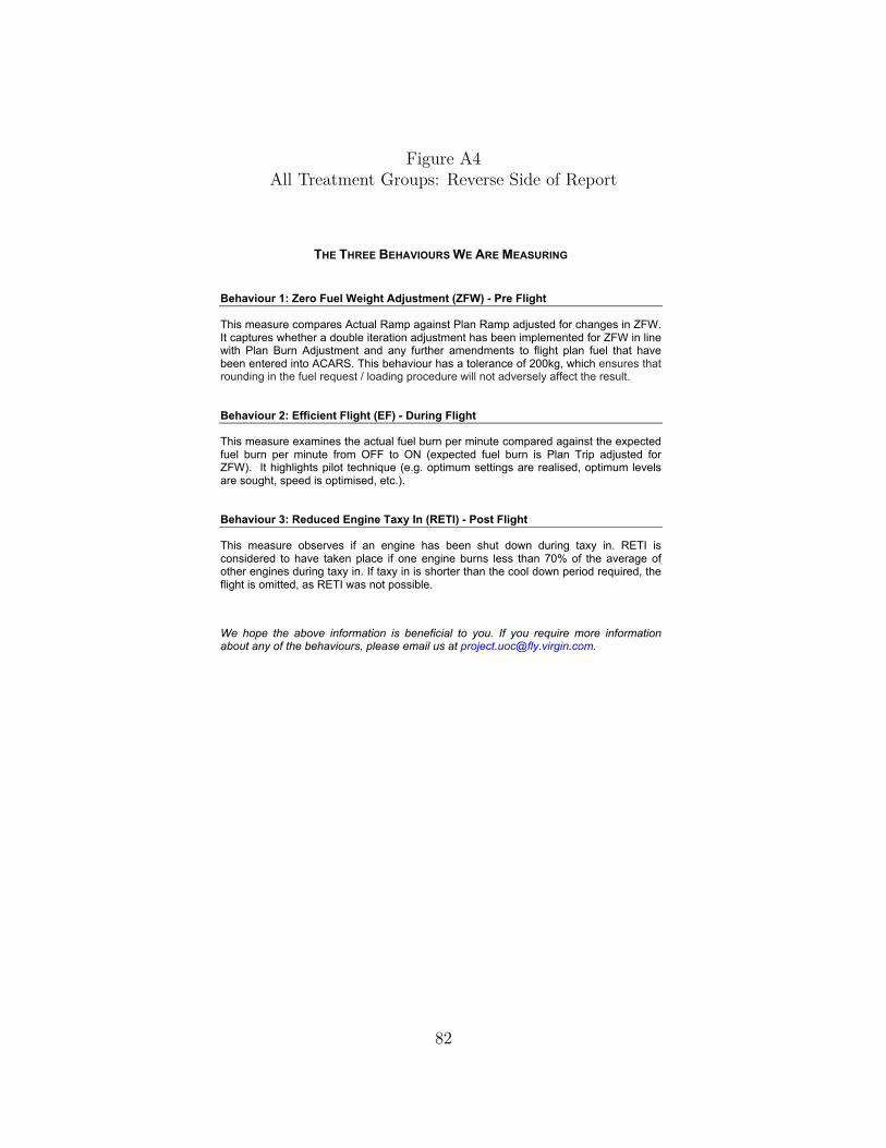
Figure A4All Treatment Groups: Reverse Side of Report

THE THREE BEHAVIOURS WE ARE MEASURING

Behaviour 1: Zero Fuel Weight Adjustment (ZFW) - Pre Flight

This measure compares Actual Ramp against Plan Ramp adjusted for changes in ZFW. It captures whether a double iteration adjustment has been implemented for ZFW in line with Plan Burn Adjustment and any further amendments to flight plan fuel that have been entered into ACARS. This behaviour has a tolerance of 200kg, which ensures that rounding in the fuel request / loading procedure will not adversely affect the result. Behaviour 2: Efficient Flight (EF) - During Flight

This measure examines the actual fuel burn per minute compared against the expected fuel burn per minute from OFF to ON (expected fuel burn is Plan Trip adjusted for ZFW). It highlights pilot technique (e.g. optimum settings are realised, optimum levels are sought, speed is optimised, etc.). Behaviour 3: Reduced Engine Taxy In (RETI) - Post Flight

This measure observes if an engine has been shut down during taxy in. RETI is considered to have taken place if one engine burns less than 70% of the average of other engines during taxy in. If taxy in is shorter than the cool down period required, the flight is omitted, as RETI was not possible.

We hope the above information is beneficial to you. If you require more information about any of the behaviours, please email us at project.uoc@fly.virgin.com.

82

D Appendix IV: Alternative Method for Data-SupportedFuel Savings Estimates

To provide robustness to the data-supported estimates discussed in section 3.3, we providean alternative measure of fuel savings derived from the data where savings are attributeddirectly to each of the three behaviors targeted in the study. For Fuel Load, we measure thedeviation of the actual fuel load from the “ideal” fuel load—the latter stemming from thedouble iteration calculation. We identify the average group-level deviation, which is positiveif the captain over-fuels relative to the ideal. We then estimate average fuel savings perflight for each treatment group, which entails summing the treatment’s effect on per-flightfuel savings from Fuel Load with the control group’s per-flight fuel savings from Fuel Load(the Hawthorne effect; see Table A9). In doing so, we assume that the Hawthorne effectis constant across groups. On average, captains in the control group decreased fuel loadrelative to the ideal by 177.7 kg, those in the information group by 148.5 kg per flight, thosein the targets group by 190.5 kg per flight, and those in the prosocial group by 208.8 kg perflight.61

Similarly, for Efficient Flight, we examine changes in captains’ fuel use relative to the“ideal” fuel use, or the anticipated fuel use according to the flight plan (adjusted for updatesmade during Fuel Load). We find that captains in the control, information, targets, andprosocial groups reduced in-flight fuel use by 256.1, 280.1, 361.1, and 329.9 kg per flight,respectively. Finally, for Efficient Taxi, we examine changes to fuel use during taxi-in.Fuel savings per flight amounted to 17.0 kg, 20.8 kg, 21.9 kg, and 11.8 kg for the control,information, targets, and prosocial incentives groups, respectively.

As a next step, we take these group-level effects and scale them up by the number of flightsper treatment group. Put differently, total savings for a given treatment cell are the sum ofthe per-flight fuel savings for each behavior (i.e., the sum of the average treatment effect andaverage Hawthorne effect) multiplied by the number of unique flights during the experimentalperiod flown by captains in that group. Results from this exercise are presented in Table

61When we instead consider the regression that does not control for a linear time trend, we find a slightdifference in the implementation of the behaviors, but as we see from Table A10, the fuel savings estimates arevery similar (savings are slightly larger in the specification that does not control for a linear time trend). Thatis, the pre-experimental trend whereby captains were increasingly implementing Efficient Taxi is accountedfor in column (6), so that the estimates reveal an additional fuel savings that derive from the experiment,holding this trend constant. Similarly, the trend increases fuel savings attributable to the experiment forFuel Load and decreases such estimates for Efficient Flight. In aggregate, the fuel savings across the twospecifications are nearly identical.

83

A10. Using the data-supported estimates, our interventions led to roughly 6.51 million kg infuel savings in aggregate. Using the same conversions as above (see Table 9), total savingscorrespond to cost savings of $5.12 million (equivalent to a reduction of 0.53% of overall fuelcosts) and CO2 savings of 20.5 million kg.

84

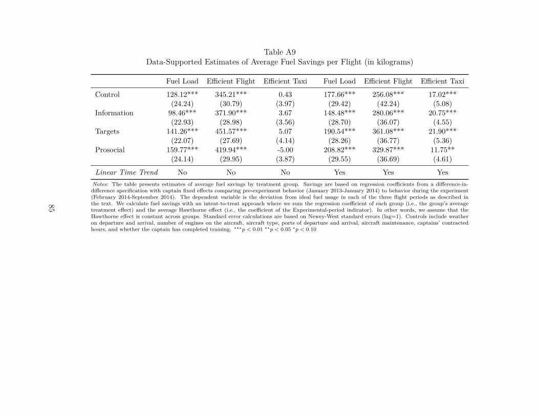
Table A9Data-Supported Estimates of Average Fuel Savings per Flight (in kilograms)

Fuel Load Efficient Flight Efficient Taxi Fuel Load Efficient Flight Efficient Taxi

Control 128.12*** 345.21*** 0.43 177.66*** 256.08*** 17.02***(24.24) (30.79) (3.97) (29.42) (42.24) (5.08)

Information 98.46*** 371.90*** 3.67 148.48*** 280.06*** 20.75***(22.93) (28.98) (3.56) (28.70) (36.07) (4.55)

Targets 141.26*** 451.57*** 5.07 190.54*** 361.08*** 21.90***(22.07) (27.69) (4.14) (28.26) (36.77) (5.36)

Prosocial 159.77*** 419.94*** -5.00 208.82*** 329.87*** 11.75**(24.14) (29.95) (3.87) (29.55) (36.69) (4.61)

Linear Time Trend No No No Yes Yes YesNotes: The table presents estimates of average fuel savings by treatment group. Savings are based on regression coefficients from a difference-in-difference specification with captain fixed effects comparing pre-experiment behavior (January 2013-January 2014) to behavior during the experiment(February 2014-September 2014). The dependent variable is the deviation from ideal fuel usage in each of the three flight periods as described inthe text. We calculate fuel savings with an intent-to-treat approach where we sum the regression coefficient of each group (i.e., the group’s averagetreatment effect) and the average Hawthorne effect (i.e., the coefficient of the Experimental-period indicator). In other words, we assume that theHawthorne effect is constant across groups. Standard error calculations are based on Newey-West standard errors (lag=1). Controls include weatheron departure and arrival, number of engines on the aircraft, aircraft type, ports of departure and arrival, aircraft maintenance, captains’ contractedhours, and whether the captain has completed training. ∗∗∗p < 0.01 ∗∗p < 0.05 ∗p < 0.10

85

Table A10Data-Supported Estimates of Fuel Savings by Behavior (in tons)

(1) (2) (3) (4) (5) (6)Fuel Load Efficient Flight Efficient Taxi Fuel Load Efficient Flight Efficient Taxi

Control 425.48*** 1,146.46*** 1.45 586.70*** 850.432*** 56.52***(80.51) (102.26) (13.17) (97.71) (140.27) (16.87)

Information 327.88*** 1,238.44*** 12.21 494.45*** 932.59*** 69.11***(76.37) (96.51) (11.86) (95.56) (121.46) (15.15)

Targets 426.03*** 1,361.95*** 15.28 574.66*** 1089.04*** 66.05***(66.58) (83.53) (12.50) (85.24) (110.89) (16.15)

Prosocial 520.53*** 1,368.16*** -16.30 680.33*** 1074.74*** 38.29**(78.65) (97.58) (12.60) (96.29) (119.55) (15.03)

Fuel Savings fromBehavior Change 1,699.91 5,115.01 12.63 2,336.14 3,946.80 229.96

Total Fuel Savings 6,827.55 6,512.90

Linear Time Trend No No No Yes Yes YesNotes: The table presents estimates of fuel savings for each targeted behavior by treatment group. Savings are based on regression coefficients from adifference-in-difference specification with captain fixed effects comparing pre-experiment behavior (January 2013-January 2014) to behavior during theexperiment (February 2014-September 2014). The dependent variable is the deviation from ideal fuel usage in each of the three flight periods as de-scribed in the text. We calculate fuel savings with an intent-to-treat approach where the regression coefficient of each group (i.e., the group’s averagetreatment effect) and the average Hawthorne effect (i.e., the coefficient of the Experimental-period indicator) are multiplied by the number of flights ineach group (3321, 3330, 3016, and 3258 respectively). In other words, we assume that the Hawthorne effect is proportional to the number of flights.Standard error calculations are based on Newey-West standard errors (lag=1). Controls include weather on departure and arrival, number of engineson the aircraft, aircraft type, ports of departure and arrival, aircraft maintenance, captains’ contracted hours, and whether the captain has completedtraining. ∗∗∗p < 0.01 ∗∗p < 0.05 ∗p < 0.10

86

E Appendix V: Survey Materials

E.1 Risk Preference Elicitation

87

E.2 Charitable Donations

88

E.3 Job Satisfaction

89