A new approach to constructing high resolution time scales with estimates of resolving power for the Early Paleozoic

Peter M. Sadler

Dept. of Earth Sciences, University of California Riverside, Riverside, CA92521, USA

Roger A. Cooper Institute of Geological and Nuclear Sciences, PO Box 30368, Lower Hutt, New Zealand

Michael J. Melchin

Dept. of Earth Sciences, St. Francis Xavier University, Antigonish, NS B2G 2VG, Canada

SUPPLEMENTARY ONLINE DATA Contents 1. Data search strategy 2. Comments on the composite sequence, placement of zone boundaries . . . 3. Table of zone age and duration calibrations. 4. Table of radiometric dates used for calibration and testing the proxy time scale. 5. Alphabetical list of sections by region. 6. List of references for sections.

1. DATA SEARCH STRATEGY. Range chart data were drawn from an extensive search of published and grey literature. We used a range of on-line databases and search engines (Georef, Melvyl, Google, JStor, GSW). We physically browsed private reprint collections and the libraries of several research institutions (U.C. Riverside, U.C. Berkeley, U.C. Los Angeles, MIT, Harvard, Purdue, IGNS, U. Cincinnati). We included as many taxa as possible from every measured section, regardless of whether or not they are generally accepted as useful for correlation. Taxa were excluded only if their taxonomic integrity is in doubt, especially where qualified by 'cf.' or '?.' By contrast, the ‘aff.’ attribute signifies a taxon that is likely new and often contributes to the correlation of sections in the publication that uses the open nomenclature; such taxa were differentiated according to the attributing author and date, then included in the compositing process. Indefinite specific assignments (‘sp.’) were included only for extremely rare genera. We have attempted to identify and reconcile synonyms from the faunal lists. The 1,928 taxa used in the largest sequencing exercises are based on a total taxon database of 3,121 names, including synonyms. Unrecognized synonyms waste valuable information but do not generate false correlations. More difficult to recognize are misidentifications and names that encompass

1

DR2008252

more than one species. These can falsely extend ranges and, in extreme situations, cause miscorrelations. Our database will certainly not be free from such flaws. They contribute to the stratigraphic uncertainty in locating zone boundaries in the scaled composite sequence. Some species in our composite sections will inevitably be broader in scope than recognized by individual taxonomists.

2. COMMENTS ON THE COMPOSITE SEQUENCE, PLACEMENT OF ZONE BOUNDARIES, AND ESTIMATION OF UNCERTAINTY INTERVALS.

During the course of this project, we have built composite sections at various stages, as the database has increased in size. Composite sections are labeled by the number of local sections involved in its construction. Hence composite-198 refers to the composite of 198 sections, used by us in construction of the Ordovician and Silurian timescales, in Webby et al. (2004) and in Gradstein et al. (2004). Composites have been built at the following stages in the expansion of the database: 177, 198, 215, 232, 256, 262, and 430 sections. They provide a test of the stability of the timescale as additional data are added (Sadler et al. this paper, fig. 6). In addition, a further composite was constructed from the largest data set culled to remove half of all sections, as explained in Sadler et al. (this paper). It is labeled composite-214. In the final timescale, we used the composite-256 for the Silurian and composite-214 for the Ordovician, as these gave the best accordance with the expected stratigraphic distribution of events (‘preferred’ calibration, Sadler et al, this paper, table 1). In both the Ordovician and Silurian, a number of events have been placed in the composite sequence by the optimizing procedure at a level that differs from that expected, from our knowledge of regional zonal sequences. There are several possible reasons for this other than error in data entry. 1. An obvious source of misplacement is taxonomic misidentification (or regional differences in taxonomic practice) in one or more levels in one or more sections. False coexistences can be created which will force a taxon range beyond the limits of its valid range during the constraining part of the procedure. Although we have revised many taxon lists in an attempt to remove obvious misidentifications and synonymies (with help from Dr. Charles Mitchell), our database will certainly still contain errors. 2. Some events are nearly unconstrained in the sense that they are found only at the base (for first appearances) or top (for last appearances) of a single section, and with few co-existing taxa. Unconstrained first-appearance events can ‘sink’ down-sequence and unconstrained last-appearance events ‘float’ up-sequence for considerable distances. Such ‘drifters’ are generally easy to recognize because they are so far out of position and thus are clearly isolated. They were considerably reduced in number from composite 198 to composite 256. The increased number of sections in the larger composites reduces the likelihood of such extreme and exclusive occurrences. For the composites 431 and 214 we added a simple containment strategy: taxa recorded by a single occurrence at the top or base of a section were entered as two occurrences, separated by one centimeter. This tied one range end into the section (which is correct), and

2

prevented the other range end from drifting without extending the range and, thus, adding to the number of implied coexistences or first-appearance below last-appearnce pair-wise sequences. 3. A secondary objective function penalizes for co-existing taxa that are implied by the correlation but not observed in any section. It is used to help with seriation, the task of sorting into correct order short-ranging sections that do not overlap in time. This penalty works with the range extension penalty, because shorter ranges generate fewer coexistences but it tends to move loosely constrained taxa into the nearest diversity minimum if possible. This is one instance in which our routines risk over-fitting the data to an objective function. To minimize over-fitting, the weight assigned to this secondary term in the objective function is only 1/100th of the main range-extension term. 4. Lazarus taxa are those known from two disjunct ranges separated by a significant gap in time. This pattern may be real or an artifact of taxonomic practice. Like spatial provincialism, this is another pattern in the distribution of taxa which only becomes clear after a temporal sequence and correlation is established and which tends to confuse the automated recognition of the true temporal relationships. Lazarus taxa tend to condense the composite sequence if the optimization process correlates all the partial ranges. The problem is not acute unless Lazarus taxa outnumber those that are found consistently throughout their ranges. 5. The biostratigraphic sequencing problem is typically underdetermined and the solutions are not unique. There is a natural variance in event order in successive composites derived from the same data base when that data base is large with many short-ranging and non-overlapping sections, such as ours. Most events are placed within a narrow interval from composite to composite (best-fit interval, Sadler & Cooper 2003) but a small number have best-fit intervals that allow the event to appear at a widely discordant levels in some composites. In placing the zone boundaries, and identifying the stratigraphic uncertainty intervals of those boundaries (discussed in text), it was necessary, for several of the zones, to distinguish between events that are ‘out of position’ in the composite for reasons that relate to lack of constraint, and those that are at unexpected levels but still within a plausible range of ‘natural variance’. The latter were used as part of the sequence for determining the location of the zone boundaries and their uncertainty intervals, the former were ignored during boundary placement. To help in making the distinction, we used the extent to which events normally regarded as characteristic of a zone are clustered in the composite. Poorly constrained taxa tend to be loners. Some Silurian zonal species (e.g. Cystograptus vesiculosus, Spirograptus guerichi) recently have been revised. As a result, the placing of their first appearances in the composite are at slight variance with some regional zonal schemes or, as in the case of M. turriculatus, the first appearance is now uncertain. The FAD of M. spiralis is taken in much of Europe to mark the base of the M. spiralis Zone. But the species is known to range much lower in other parts of the world. As used here it is more of an acme zone than a range zone. The Wenlock is the most finely resolved part of our entire Ordovician and Silurian time scales. Boundaries are generally clearly defined, despite the provincialism that persisted at this time. The most problematic part of the Silurian composite is the Ludlow, caused by a combination of a lack of good stratigraphic sections globally, marked provincialism and systematic problems. Some key zonal species are

3

missing by chance from our composite. Resolution will be improved by improved taxonomy and the inclusion of better stratigraphic sections in the database. The Australasian Comparison The test plots the Australasian rank order of events against the CONOP9 composite sequence (Fig. 5A). It yields an encouragingly high rank order correlation coefficient (Spearman's Rs = 0.9225). A better fit is achieved by locally estimated sums of squares (LOESS curve with a span factor of 0.3; multiple r2 = 0.95). Thus, the composite order of events matches well with an exhaustively collected and studied regional sequence of high reliability, at least for the Ordovician. Note that the plot includes all species common to the Australasian sequence and CONOP global composite. Some are long-ranging species such as Dichograptus octobrachiatus, Tetragraptus quadribrachiatus, Expansograptus extensus, and Cryptograptus tricornis, with irregular first and last appearances that are generally avoided for long range correlation. An even better correlation would be achieved in Fig. 5A if these species were excluded. They are included here because our intention here is to minimize subjective censoring of data. Zone Boundaries The long Ordovician Lancefieldian La2 Zone is divided into lower and upper parts. Lower boundaries for some zones - Pendeograptus fruticosus (Be2-4), I. victoriae maximodivergens (Ca4), Oncograptus upsilon (Ya1) and Dicellograptus gravis (Ea4) - could not be unambiguously determined in some early composites. The base of one zone (Zone Bo4, Normalograptus extraordinarius) was defined at the last appearance of a proxy taxon, Diceratograptus mirus. In the Silurian, the zones of Koren’ et al. (1996) are used, as modified by one of us (MJM). The zones of Monograptus bouceki–M. perneri, Monograptus riccartonensis, and Neocucullograptus kozlowskii, B. cornuatus-P. podoliensis, could not be distinguished in the Silurian scale. Stage boundaries are readily located in the zonal succession in both periods as all are based on either graptolite or conodont events. Error Estimation in Gradstein et al. (2004) Our method of estimating errors on ages of stage and zone boundaries differs from that used by Agterberg in Gradstein et al. (2004). Agterberg fitted a cubic spline curve through points representing the means of individual dated samples, on a time axis plotted against a stratigraphic axis (our composite-198). Points were weighted in inverse proportion to their combined analytical (two sigma) and stratigraphic error. Uncertainty was calculated from the squared deviances of points by the MLFR (maximum likelihood of a function relationship) method and thus incorporates both stratigraphic and analytical components. An average for the Ordovician and Silurian stage boundaries was found, and error on individual points was then adjusted by “sample point distribution” according to age. This approach gives equal importance to the stratigraphic and analytical components of uncertainty at all scales within the Ordovician and Silurian. In contrast, we regard the composite as providing the most reliable spacing of zone boundaries over the short term, that is, over the span of several zones (up to 5-10 m.y.). Radiometric data provide better control over the longer term. Cumulative error in the composite over long spans is compensated for by the polynomial regression fitted through the dated points. As a result, our errors on stage and zone boundaries (Table 1) are purely stratigraphic and are considerably less than those given in Gradstein et al. (2004).

4

Gradstein, F. M., Ogg, J. G., and Smith. A. G., 2004, A Geologic Time Scale 2004: Cambridge University Press, 598 p.

Webby, B. D., Paris, F., Droser, M. L., and Percival, I. G., 2004, The Great Ordovician Biodiversification Event. Columbia University Press, New York, 484 p.

5

3. CALIBRATED AGES AND DURATIONS OF ZONES Tables 1A and 1B list the calibrated ages of zone boundaries for four composite sections and the preferred calibration that is a combination of composite 214 (for the Ordovician) and composite 256 (for the Silurian). Table 1A lists the stages and proxy taxa for each zone; the same qualities apply to zones in Table 1B. TABLE 1A Age of Base (Ma) in Composite

Stage Zone Proxy taxon 198 256 431 214

Lochkovonian Monograptus yukonensis Monograptus yukonensis 414.73 413.42 414.93 -

Lochkovonian M. hercynicus hercynicus M. hercynicus hercynicus 416.34 415.57 416.65 -

Base Devonian Monograptus uniformis M. uniformis parangustidens 417.23 416.90 417.75 -

Pridoli Monograptus transgrediens

Pseudomonocl. cinctutus 418.00 418.45 419.15 -

Pridoli Monogr. bouceki - perneri - 418.08 - 419.55 -

Pridoli Monograptus lochkovensis

Monograptus prognatus 418.90 418.87 419.66 -

Pridoli N. lochkov. branikensis N. lochkovensis branikensis 418.93 418.93 - -

Pridoli Neo. parultimus - ultimus Neocolonograptus parultimus 419.68 420.31 420.82 418.94

Ludfordian Monograptus formosus Monograptus formosus 420.18 420.44 - 419.12

Ludfordian N.kozlowskii-B.cornuat/podol.

Bohemograptus cornuatus - - 420.91 419.77

Ludfordian S. leintwardensis-linearis S. leintwardensis incipiens 421.98 421.27 421.66 420.90

Gorstian Lobograptus scanicus Saetograptus wandalensis 423.01 422.35 422.42 -

Gorstian Neodiversograptus nilssoni

Neodiversograptus nilssoni 423.49 422.65 422.90 -

Homerian C. ludensis Colonograptus ludensis 423.88 422.81 - 421.41

Homerian C.? praedeubeli/deubeli Colonograptus? praedeubeli 424.49 423.09 423.59 422.19

Homerian P. dubius parvus-G.nassa

Pristiograptus dubius parvus 424.75 424.02 424.19 423.12

Homerian Cyrtograptus lundgreni Cyrtograptus lundgreni 426.15 424.92 424.54 424.57

Scheinwoodian C. perneri-M.transgrediens Cyrtograptus perneri 426.53 425.34 425.81 424.82

Scheinwoodian C.rigidus-M.belophorus-anten.

Monograptus antennularius 427.25 426.06 426.17 425.46

Scheinwoodian Monograptus Monograptus 427.47 - 426.25 425.59

6

riccartonensis riccartonensis

Scheinwoodian Cyrtograptus murchisoni Cyrtograptus murchisoni 427.76 426.53 426.43 426.01

Scheinwoodian Cyrtograptus centrifugus Cyrtograptus centrifugus 428.27 427.07 427.97 426.54

Scheinwoodian Cyrtograptus insectus Cyrtograptus insectus 428.39 427.52 427.99 426.72

Telychian Cyrtograptus lapworthi Cyrtograptus lapworthi 429.22 429.01 429.15 427.91

Telychian O.spiralis interval Oktavites falx 430.90 429.43 430.40 429.29

Telychian M. crenulata-griestoniensis

Monoclimacis griestoniensis 431.86 430.44 430.76 430.11

Telychian Monograptus crispus Petalolithus wilsoni 432.54 431.66 431.83 430.39

Telychian Spirograptus turriculatus Torquigraptus proteus 433.81 432.50 433.91 431.97

Telychian Spirograptus guerichi Spirograptus guerichi 435.87 434.90 436.05 434.39Aeronian Simulograptus sedgwicki Monograptus distans 436.46 435.85 436.38 435.81

Aeronian Lituigraptus convolutus Lituigraptus convolutus 437.07 436.97 438.00 436.26

Aeronian M.argenteus-P.leptotheca

Pribylograptus leptotheca 437.51 437.46 438.28 436.57

Aeronian D.pectinatus-D.triangulatus

M. triangulatus triangulatus 438.68 439.37 439.03 438.22

Rhuddinian Coronograptus cyphus Coronograptus cyphus 440.22 440.18 440.58 439.97

Rhuddinian Orthograptus vesiculosus Dimorphograptus elongatus 441.13 442.42 441.89 442.12

Rhuddinian Parakidograptus acuminatus

P.acuminatus acuminatus 441.95 444.06 442.47 442.68

Base Silurian Akidograptus ascensus Akidograptus ascensus 443.24 444.40 442.85 443.41

Bolindian 5 Normalograptus persculptus

Normalograptus persculptus 444.29 445.28 444.01 444.13

Bolindian 4 Normalogr. extraordinarius

Diceratograptus mirus LAD 445.12 446.36 446.18 444.67

Bolindian 3 Paraorhograptus pacificus

Paraorthograptus pacificus 447.05 448.00 447.03 446.20

Bolindian 2 pre-pacificus zone Climacograptus missilis 448.31 449.09 447.15 447.87

Bolindian 1 Climacograptus? uncinatus

Climacograptus uncinatus 449.73 449.64 448.04 448.57

Eastonian 4 Dicellograptus gravis Dicellograptus gravis - - 448.91 448.96Eastonian 3 Dicranograptus kirki Pleurograptus linearis 452.32 452.83 450.38 449.73

Eastonian 2 Diplacanthogr. spiniferus Diplacanthograptus spiniferus 454.27 453.28 453.23 452.21

Eastonian 1 Diplacanthogr. lanceolatus

Orthograptus pageanus 456.12 455.43 455.28 455.29

Gisbornian 2 Orthograptus calcaratus Lasiograptus costatus 458.00 458.07 455.67 456.35

Gisbornian 1 Nemagraptus gracilis Nemagraptus gracilis 460.53 460.76 458.93 460.86

Darriwil. 4a-b Archiclimacogr. riddellensis Pterograptus elegans 462.77 464.14 463.02 463.04

Darriwilian 3 Pseudoclimacogr. decoratus

Pseudoclimacogr. decoratus 464.94 465.08 466.66 467.94

7

Darriwilian 2 Undulograptus intersitus Pseudobryograptus incertus 466.29 465.83 466.94 469.57

Darriwilian 1 Undulograptus austrodentatus

Undulograptus austrodentatus 468.08 468.38 469.27 470.54

Yapeenian 2 Cardiograptus morsus Cardiogr. morsus (narrow) 468.86 469.30 469.50 471.21

Yapeenian 1 Oncograptus upsilon Paraisogr. caduceus caduceus - - 469.50 472.36

Castlemain. 4 I. victoriae maximodivergens Arienigr. dumosus A - - 469.66 473.01

Castlemain. 3 Isograptus victoriae maximus

Isograptus victoriae maximus 469.99 469.41 471.08 473.44

Castlemain. 2 Isograptus victoriae victoriae

Isograptus victoriae victoriae 470.63 470.39 473.49 473.91

Castlemain. 1 Isograptus victoriae lunatus

Isograptus victoriae lunatus 471.96 471.78 473.62 475.44

Chewton. 1-2 Didymograptellus protobifidus Acrograptus gracilis 473.89 472.70 475.06 476.68

Bendigonian 4 Pendeograptus fruticosus 3

Expansograptus procumbens - 472.84 475.08 476.80

Bendigonian 3 Pendeograptus fruticosus 3&4 Laxograptus shellyi - 472.91 475.22 476.88

Bendigonian 2 Pendeograptus fruticosus 4 P. fruticosus 3 - 472.96 475.53 477.62

Bendigonian 1 P. fruticosus + T.approximatus

Pendeograptus crassus 476.81 475.57 478.46 481.45

Lancefield. 3 Tetragraptus approximatus T. decipiens bipatens 479.24 478.40 481.99 481.73

Lancefield. 2b Araneograptus murrayi Paradelograptus pritchardi 484.47 481.27 484.85 483.70

Lancefield. 2a Aorograptus victoriae Temnograptus regularis 486.92 486.95 486.72 485.15

Lancefield. 1b Psigraptus lenzi Psigraptus magnus 487.36 487.22 487.07 486.96

Lancefield. 1a R.scitulum & Anisograptus

Anisograptus ruedemanni 488.66 488.63 489.12 -

pre-Lancefield. R. flabelliformis parabola R. flabelliformis parabola 489.80 490.01 490.70 -

Base Ordovician Iapetognathus fluctivagus Iapetognathus fluctivagus 489.97 490.88 490.78 -

8

TABLE 1B Preferred Stratigraphic Zone Age Duration Age error as Zone calibration uncertainty duration error error fraction of (Ma) (m.y.) (m.y.) (m.y.) (m.y.) zone duration Monograptus yukonensis 413.42 +0/-0.01 - 0.01 - - M. hercynicus hercynicus 415.57 +0/-0.14 2.15 0.14 0.14 0.07Monograptus uniformis 416.90 +0/-0.12 1.33 0.12 0.12 0.09Monograptus transgrediens 418.45 +0/-0.15 1.55 0.15 0.15 0.10Monogr. bouceki - perneri - - - - - - Monograptus lochkovensis 418.87 +0/-0 0.42 0.00 0.00 0.00N. lochkov. branikensis 418.93 +0/-0.01 0.06 0.01 0.01 0.16Neo. parultimus - ultimus 420.31 +0/-0.02 1.37 0.02 0.02 0.01Monograptus formosus 420.44 +0.02/-0.02 0.13 0.04 0.02 0.16N.kozlowskii-B.cornuat/podol. - - - - - - S. leintwardensis-linearis 421.27 +0/-0.18 0.84 0.18 0.20 0.24Lobograptus scanicus 422.35 +0/-0.6 1.08 0.60 0.60 0.55Neodiversograptus nilssoni 422.65 +0/-0 0.29 0.00 0.00 0.00C. ludensis 422.81 +0/-0.02 0.17 0.02 0.02 0.12C.? praedeubeli/deubeli 423.09 +0/-0 0.27 0.00 0.00 0.00P. dubius parvus-G.nassa 424.02 +0/-0.44 0.93 0.44 0.44 0.47Cyrtograptus lundgreni 424.92 +0/-0.03 0.90 0.03 0.03 0.03C. perneri-M.transgrediens 425.34 +0/-0.02 0.42 0.02 0.02 0.05C.rigidus-M.belophorus-anten. 426.06 +0/-0.14 0.72 0.14 0.14 0.19Monograptus riccartonensis - - - - - - Cyrtograptus murchisoni 426.53 +0.03/-0 0.47 0.03 0.00 0.00Cyrtograptus centrifugus 427.07 +0/-0.07 0.54 0.07 0.10 0.18Cyrtograptus insectus 427.52 +0/-0.36 0.45 0.36 0.36 0.81Cyrtograptus lapworthi 429.01 +0/-0.95 1.49 0.95 0.95 0.64O.spiralis interval 429.43 +0.24/-0 0.43 0.24 0.00 0.00M. crenulata-griestoniensis 430.44 +0.29/-0.36 1.01 0.65 0.60 0.59Monograptus crispus 431.66 +0/-0.03 1.22 0.03 0.32 0.26Spirograptus turriculatus 432.50 +0/-0.75 0.83 0.75 0.75 0.90Spirograptus guerichi 434.90 +0.04/-0.09 2.40 0.13 0.09 0.04Simulograptus sedgwicki 435.85 +0/-0.38 0.95 0.38 0.42 0.44Lituigraptus convolutus 436.97 +0.22/-0.03 1.12 0.25 0.03 0.03M.argenteus-P.leptotheca 437.46 +0.09/-0.01 0.49 0.10 0.23 0.47D.pectinatus-D.triangulatus 439.37 +0/-0.56 1.91 0.56 0.65 0.34Coronograptus cyphus 440.18 +0/-0.22 0.81 0.22 0.22 0.27Orthograptus vesiculosus 442.42 +0/-0.39 2.24 0.39 0.39 0.17Parakidograptus acuminatus 442.68 +0/-0 0.26 0.00 0.05 0.19Akidograptus ascensus 443.41 +0/-0 0.73 0.00 0.00 0.00Normalograptus persculptus 444.13 +0/-0 0.72 0.00 0.00 0.00Normalogr. extraordinarius 444.67 +0.01/-0 0.54 0.01 0.00 0.00Paraorhograptus pacificus 446.20 +0/-0 1.53 0.00 0.01 0.01pre-pacificus zone 447.87 +0/-0 1.67 0.00 0.00 0.00Climacograptus? uncinatus 448.57 +0.14/-0 0.70 0.14 0.00 0.00Dicellograptus gravis 448.96 +0/-0 0.39 0.00 0.14 0.36

9

Dicranograptus kirki 449.73 +0.39/-0 0.77 0.39 0.00 0.00Diplacanthogr. spiniferus 452.21 +0.26/-1.31 2.48 1.57 1.70 0.69Diplacanthogr. lanceolatus 455.29 +0/-0.44 3.08 0.44 0.70 0.23Orthograptus calcaratus 456.35 +0.23/-0 1.06 0.23 0.00 0.00Nemagraptus gracilis 460.86 +0.54/-1.01 4.51 1.55 1.24 0.27Archiclimacogr. riddellensis 463.04 +0.29/-0 2.18 0.29 0.54 0.25Pseudoclimacogr. decoratus 467.94 +0.37/-0.39 4.90 0.76 0.68 0.14Undulograptus intersitus 469.57 +0.1/-0 1.63 0.10 0.37 0.23Undulograptus austrodentatus 470.54 +0.27/-0 0.97 0.27 0.10 0.10Cardiograptus morsus 471.21 +0.05/-0 0.67 0.05 0.27 0.40Oncograptus upsilon 472.36 +0.15/-0.05 1.15 0.20 0.10 0.09I. victoriae maximodivergens 473.01 +0/-0 0.65 0.00 0.15 0.23Isograptus victoriae maximus 473.44 +0.04/-0.04 0.43 0.08 0.04 0.09Isograptus victoriae victoriae 473.91 +0.33/-0 0.47 0.33 0.04 0.09Isograptus victoriae lunatus 475.44 +0.17/-0 1.53 0.17 0.33 0.22Didymograptellus protobifidus 476.68 +0.12/-0 1.24 0.12 0.17 0.14Pendeograptus fruticosus 3 476.80 +0.04/-0 0.12 0.04 0.12 1.00Pendeograptus fruticosus 3&4 476.88 +0/-0 0.08 0.00 0.04 0.50Pendeograptus fruticosus 4 477.62 +0/-0.66 0.74 0.66 0.66 0.89P. fruticosus + T.approximatus 481.45 +0/-0 3.83 0.00 0.00 0.00Tetragraptus approximatus 481.73 +0.23/-0.06 0.28 0.29 0.06 0.21Araneograptus murrayi 483.70 +0.94/-0 1.97 0.94 0.23 0.12Aorograptus victoriae 485.15 +1.05/-0 1.45 1.05 0.94 0.65Psigraptus lenzi 487.22 +0.04/-0 2.07 0.76 1.71 0.83R.scitulum & Anisograptus 488.63 +0.16/-1.21 1.41 1.37 1.31 0.93R. flabelliformis parabola 490.01 +0.1/-0.66 1.38 0.76 0.82 0.59Iapetognathus fluctivagus 490.88 +0.04/-0.1 0.87 0.14 0.20 0.23

10

4. RADIOISOTOPIC DATES

In Table 2, radiometrically dated samples used for calibration and testing of the proxy time scale are listed (abbreviated from Sadler and Cooper (in Gradstein et al. 2004)). Note that the ages for Ar40-Ar39 dated samples listed in the column “Age” have been re-calibrated with the MMhb-1 monitor standard by M. Villeneuvre. Items used by Tucker and McKerrow (1995) are identified in the second column by their item number in square brackets.

11

Table 2 Ordovician to Devonian isotopic dates used for calibration

Locality Formation Comment Primary biostratgraphic age Reference AGE Type

1 K-bentonite, New York, USA.

Kalkberg Formation

Ten small fractions of 4-12 grains each; 4 give concordant analyses; all share a 207Pb-206Pb age of ~417. Weighted mean 207Pb/206Pb age 417.6 ±1.0

Conodonts in other sections of the Kalkberg Formation

Tucker et al. 1998 417.6 ±1.0 Pb-Pb

2 Felsic volcanic, Canberra, Australia, [25]

Laidlaw Volcanics

An average age from K-Ar (mineral) and Rb-Sr (whole rock and mineral) analyses, of 420.7±2.2. (SHRIMP age of 419.6 ±5.6 not used)

Interbedded with Gorstian fossiliferous seds

Wyborn et al. 1982 420.7±2.2 K-Ar and Rb-Sr

3 Bentonite, Shropshire

Middle Elton Formation

Two biotite grains with slightly "discordant" age spectra give similar total-gas 40Ar-39Ar ages (424.5 and 425 Ma). The 40Ar-39Ar weight-average plateau age of 423.7 +/-1.7 Ma is regarded as best age..

Associated with graptolitess indicative of Neodiv.nilssoni and Lobo. scanicus Zones, Gorstian

Kunk et al. (in Snelling) 1989; lanphyre et al. 1977.

426.8 ±1.7 Ar-Ar

4 Thin volcanic ash. , Welshpool, Wales, [24]

Buttington Shales

Mean 207Pb-206Pb age of "4 concordant analyses consisting of 10-20 grains per fraction analysed".

Within the zone of Monoclimacis crenulata

Tucker and McKerrow 1995, Tucker 1991 (USGS open file report)

430.1 ±2.4 Pb-Pb

5 Ash, Esquibel Island, Alaska, [23]

Descon Formation

Ar-Ar total gas age, 1200 degrees C fusion (Kunk et al. 1985)

4m above shale with graptolites of Coronogr. cyphus Zone age (Churkin et al. 1971).

Kunk et al. 1985; Churkin et al. 1971; Ross et al. 1982

436.2 ± 5 Ar-Ar

6 Ash, Dobbs Linn, [22]

Volc ash, Birkhill Shales

Mean 207Pb-206Pb of 4 concordant analyses consisting of 13-20 grains in each fraction analysed.. Ash is 6m above top of Ordovician - Toghill 1968 (not 60m as per Tucker et al. 1990 & T&McK 1995).

Coronogr. cyphus Zone Tucker et al. 1990; Ross et al. 1982 for locality; Toghill 1968.

438.7 ± 2.1 Pb-Pb

7 Ash, Dobbs Linn (Linn Branch), [21]

Hartfell Shales U-Pb age, "based on 3 concordant zircon fractions of 10-30 grains each"

Aproximately 4.5m below O/S GSSP, Paraorthograptus pacificus Zone

Tucker et al. 1990 445.7 ± 2.4 U-Pb

8 K-bentonite, Millbrig, [20a]

Millbrig K-bentonite

Mean U-Pb age of 5 concordant single grain analyses, 453.1 ±1.3 (Tucker 1992)

Phragmodus undatus Zone (lower) Bergstrom 1989, Huff et al. 1992, Tucker et al.1990

453.1 ± 1.3 U-Pb

9 K-bentonite, Millbrig (as above), [20a]

Millbrig K-bentonite

40Ar-39Ar on biotite, 451.1 ±2.1 (Kunk et al. 1985) Phragmodus undatus Zone (lower) Kunk et al. 1985 457.4 ±2.2 Ar-Ar

10 K-bentonite, Millbrig, [20b]

Diecke K-bentonite

"Mean 206Pb-238U age of 5 concordant single grain analyses", 454.5 (Tucker 1992)

Phragmodus undatus Zone (lower) Tucker 1992, Tucker and McKerrow 1995

454.5 ±0.5 U-Pb

11 Calcareous ash, Pont-y-ceunant, Bala, Wales, [19]

Base of Geli-grin

"Mean 206Pb/238U age of 454.8 ± 1.7" (Tucker 1992) Rich brachiopod, trilobite, conodont fauna. 'Longvillian' - above D.multidens , below D.clingani

Tucker et al. 1990, Tucker1992 454.8 ± 1.7 U-Pb

12 K-bentonite, Mossen Quarry, Kinnekulle, Sweden, [18]

Chasmops Limestone

40Ar-39Ar dates on biotite and sandine phenocrysts, 455.0 ± 3 (Kunk and Sutter 1984), and 454 (Kunk et al. 1988)

Conodonts, correlated by Bergstroem et al 1995:5

Kunk & Sutter 1984, Tucker & McKerrow 1995, Bergstroem et al. 1995, Leslie & Bergstroem 1995

458.3 ± 3 Ar-Ar Ar-Ar

13 K-bentonite, Mossen Quarry, Kinnekulle, Sweden, [18]

Chasmops Limestone

Mean U-Pb age of 5 concordant single grain analyses, 456.9 ±1.8 (Tucker, in Tucker & McKerrow 1995)

Conodonts, correlated by Bergstroem et al 1995:5

Kunk et al. 1988, Kunk & Sutter 1984, Tucker & McKerrow 1995, Bergstroem et al. 1995, Leslie & Bergstroem 1995

456.9 ± 1.8 U-Pb

14 Calcareous ash, Pont-y-ceunant, Bala, Wales, [19]

Base of Geli-grin

Mean 207Pb-206Pb age from 4 multigrain fractions of 457.4 ± 2.2; or mean 206Pb/238U age of 454.8 (Tucker et al. 1990)

Rich brachiopod, trilobite, conodont fauna. 'Longvillian' - above D.multidens , below D.clingani

Tucker et al. 1990 457.4 ± 2.2 Pb-Pb

15 Gritty calcareous ash, Llandindrod, centrl wales, [15]

Llanvirn Series Mean 207Pb-206Pb age of 5 concordant fractions of 1-20 grains each, give 460.4 ± 2.2

D.murchisoni immediateley below sampled ash "considered by Elles to be close to base G.teretiusculus Z"

Ross et al 1982, Tucker & McKerrow 1995

460.4 ± 2.2

16 K-bentonite, Cerro viejo, San Juan, Argentina

Los Azules Formation

Three "almost concordant" fractions (14 grains total), 1 discordant, give a well defined intercept age of 464 ±2. (Sample ARG-1, Huff et al. 1997)

10 graptolite species listed by Mitchell et al. 1998

Huff et al. 1997, Mitchell, Astini & Brussa 1998

464 ±2 U-Pb

17 Indurated bentonite, Abereiddy Bay, Wales, [14]

Lower rhyolitic tuff, Llanrian Volc Fmn

Mean of 3 concordant + 1 slightly discordant 207Pb-206Pb multigrain fractions, 464.6 ±1.8. (=76SW21 of Ross et al 1982)

Immediately overlying Cyffredin Shale is of D.murchisoni zone age (Tucker & McKerrow 1995).

Tucker et al. 1990; Hughes Jenkins & Rickards 1981

464.6 ± 1.8 Pb-Pb

18 Ash flow, Arenig Fawr, Wales, [13]

Serv Formation

Mean 207Pb-206Pb age of 2 concordant, and 1 "slightly discordant", multigrain fractions.

Underlying mudstone contains D. artus Zone graptolites

Tucker et al. 1990 465.7 ± 2.1

19 Rhyolite, Central Newfld, [12]

Cutwell Group Three small fractions give an upper intercept (207Pb-206Pb) age of 469 +5-3.

Sparse fauna of mid-continental conodonts, Histiodella holodentata ; mid-lower E.variabilis Z

Dunning & Krough 1991, Stouge 1980, pers comm.

469 +5/ -3 Pb-Pb

20 Volcanic sandstone, McLeod Brook, Cape Breton Is.

Chelsey Drive Group

Mean 206Pb/238U-207Pb/235U age of 8 multigrain discordant fractions define a concordant point at 483.3+3.9/-2.1 (0.7% discordant). Weighted mean Pb-Pb age 483±1 (with MSWD = 0.14) preferred.

Peltocare rotundiformis , Hunnegr . cf.copiosus , Adelograptus of quasimodo type

Landing et al. 1997 483±1 Pb-Pb

21 Crystal-rich volcanic sandstone, Bryn-llin-fawr, N Wales

Dollgellau Formation

Weighted mean 207Pb-206Pb date based on 17 concordant analyses of 22 fractions derived from 2 closely spaced volcaniclastic bands; indicates a maximum age for ash.

Close to top Acercare Zone. Dated ash is 4m below appearance of Rhabdinopora , and 5m below R.f. parabola . It is therefore very close to C/O boundary

Landing et al. in press Maximum age 489 ±0.6

Pb-Pb

22 Crystal-rich volcanic sandstone, Ogof-ddu, Criccieth, N Wales

Dolgellau Formation

Four nearly concordant and 5 discordant analyses from crystal rich volcaniclastic sandstone. Weighted mean dates of 4 concordant analyses = 490.9±0.5 (207Pb-206Pb); 490.7±0.7 (206Pb/238U); 490.7±0.5 (207Pb/235U). Suggested age - 491±1. Maximum age only.

Peltura scarabaeoids scarabaeoids below and P.s. westergardi above. = Lower Peltura scarabaeoides Zone

Davidek et al. 1998 Maximum age 491 ± 1

Pb-Pb, U-Pb

23 Rhyolite, Slieve Gallion, N. Ireland

Tyrone Volcanic Group

Three concordant fractions (of four crystals), from fine-grained flow-bandrd rhyolite, give a concordia age of 473±0.8 Ma.

Immediately overlying mudstone contains Isograptus victoriae lunatus

Cooper et al. in press. 473±0.8 U-Pb

12

References for radioisotopic ages used for calibration of Ordovician and Silurian scales Bergström, S. M., 1989, Use of graphic correlation for assessing event-stratigraphic significance

and trans-Atlantic relationships of Ordovician K-bentonites: Proceedings of the Academy of Sciences of the Estonian SSR. Geology, v. 38, no. 2, p. 55-60.

Bergström, S. M., Huff, W. D., Kolata, D. R., and Bauert, H., 1995, Nomenclature , stratigraphy, chemical fingerprinting, and areal distribution of some Middle Ordovician K-bentonites in Baltoscandia: Geologiska Forenigens Forhandlingar, v. 117, p. 1-13.

Cooper, M.R., Crowley, Q.G., and Rushton, A.W.A., in press, New age constraints for the Ordovician Tyrone Volcanic Group, Northern Ireland; Journal of the Geological Society of London.

Dunning, G. R., and Krogh, T. E., 1991, Stratigraphic correlation of the Appalachian Ordovician using advanced U-Pb zircon geochronology techniques: Geological Survey of Canada Paper, 90-9, p. 85-92.

Huff, W. D., Bergström, S. M., and Kolata, D. R., 1992, Gigantic Ordovician volcanic ash fall in North America and Europe: biological, tectonomagmatic, and event-stratigraphic significance: Geology, v. 20, p. 875-878.

Hughes, C. P., Jenkins, C. J., and Rickards, R. B., 1982, Abereiddy Bay and the adjacent coast, in Bassett, M. G., ed., Geological escursions in Dyfed, south-west Wales: Cardiff, National Museum of Wales, p. 51-63.

Huff, W. D., Davis, D., Bergström, S. M., Krekeler, M. P. S., Kolata, D. R., and Cingolani, C., 1997, A biostratigraphically well-constrained K-bentonite U-Pb zircon age of the lowermost Darriwilian Stage (Middle Ordovician) from the Argentine Precordillera: Episodes, v. 20, no. 1, p. 29-33.

Kunk, M. J., and Sutter, J. F., 1984, 40Ar/39Ar age spectrum dating of biotites from Middle Ordovician bentonites, eastern North America, in Brtton, D. L., ed., Aspects of the Ordovician System: Palaeontological contributions from the University of Oslo, Universitetsforlaget.

Kunk, M. J., Sutter, J., Obradovitch, J. D., and Lanphere, M. A., 1985, Age of biostatigraphic horizons within the Ordovician and Silurian Systems, in Snelling, N. J., ed., The chronology of the geological record.: Geological Society Memoir: Oxford, Blackwell Scientific Publications, p. 89-92.

Kunk, M. J., Samson, S. D., and Roddick, J. C., 1988, 40A/39A age spectrum dating of biotite and sanidine and U-Pb dating of zircon of mid-Ordovician bentonites from Sweden: a comparison with results from eastern North America, Abstracts and Program: 5th International Symposium on the Ordovician System: St Johns, Newfoundland, p. 49.

Leslie, S. A., and Bergström, S. M., 1995, Revision of the North American late Middle Ordovician standard stage classification and timimg of the Trenton transgression based on K-bentonite bed correlation, in Cooper, J. D., Droser, M. L., and Finney, S. C., eds., Ordovician Odyssey: short papers for the Seventh International Symposium on the Ordovician System: Book: Fullerton, Pacific Section Society for Sedimenatry Geology (SEPM), p. 49-54.

Landing, E., Bowring, S. A., Davidek, K. L., Rushton, A. W. A., Fortey, R. A., and Wimbledon, W. A. P., 2000, Cambrian-Ordovician boundary age and duration of the lowest Ordovician

Tremadoc Series based on U-Pb zorcon dates from Avalonian Wales: Geological Magazine, v. 137, p. 485-494.

13

Landing, E., Bowring, S. A., Fortey, R. A., and Davidek, K. L., 1997, U-Pb zorcon date from Avalonian Cape Breton Island and geochronologic calibration of the Early Ordovician: Canadian Journal of Earth Sciences, v. 34, p. 724-730.

Lanphere, M. A., Churkin, M. J., and Erberlein, G. D., 1977, Radiometric age of the Monograptus cyphus graptolite zone in south-eastern Alaska - An estimate of the age of the Ordovician-Silurian boundary: Geological Magazine, v. 114, p. 15-24.

Ross, R. J., Naeser, C. W., Izett, G. A., Obradovitch, J. D., Bassett, M. G., Hughes, C. P., Cocks, L. R. M., Dean, W. T., Ingham, K. K., Jenkins, C. J., Rickards, R. B., Sheldon, P. R., Toghill, P., Whittington, H. B., and Zalasiewicz, J., 1982, Fission-track dating of British Ordovician and Silurian stratotypes: Geological Magazine, v. 119, p. 135-153.

Toghill, P., 1968, The graptolite assembalges and zones of the Birkhilll Shales (Lower Silurian) at Dobb's Linn: Palaeontology, v. 11, no. 5, p. 654-668.

Tucker, R. D., 1992, U-Pb dating of plinian-eruption ashfalls by the isotope dilution method: a reliable and precise tool for time-scale calibration and biostratigraohic correlation: Abstracts and Programs, v. 24, no. 7, p. A198.

Wyborn, D., Owen, M., Compston, W., and McDougall, I. M., 1982, The Laidlaw Volcanics: a Late Silurian point on the geological time scale: Earth and Planetary Science Letters, v. 59, p. 90-100.

14

5. ALPHABETICAL LIST OF SECTIONS BY REGION Graptolite-bearing stratigraphic sections used for the construction of composite sequences, and time scales are listed below. Italics indicate zonal composite “pseudosections.” Asterisks identify sections selected for composite-214. The sequencing algorithms can usefully incorporate information from what we term “pseudo sections.” These devices supply information about observed superpositional order on scales other than true rock thickness. Dated events, for example, can conveniently be included twice: each in a real section, with associated faunas, and also arrayed together in a single pseudo-section with an age scale. Then it is a simple matter to cross-plot all rescaled and composite sections against a time scale. We also include some range charts drawn against a scale of traditional zones and sub zones. These zonal compilations allow access to information in areas where the details of individual sections have not been published. All pseudo sections are excluded from the scaling process. Their usage in the sequencing task also mandates the sensu-stricto ordering rules – two taxa can be assumed to coexist only if both ranges cross the same boundary between two zones or two formations. That is, all faunal samples whether reported from a single bed, zone, or formation are treated as warily as if they were known to mix all finds from a significant interval of time. Sometimes the thickness scales of two published range charts for the same section are difficult to reconcile. We prefer to enter such charts as separate sections, leaving the sequencing rules to reconcile them. Where the same marker bed can be reliably identified in both publications, it may be entered in both sections to constrain their reconciliation. Arctic North America Arctic Llandovery composite*, Melchin, 1989. Abbott River*, Canadian Arctic Islands; Lenz, 1995; Lenz and Kozlowska-Dawidziuk, 2002. Abbott River 98*, 95*, 97*, and 91*, Canadian Arctic Islands; ; Lenz and Kozlowska-

Dawidziuk, 2002. Baird Mountains, Alaska; Carter and Tailleur, 1984. Blackstone River, Canadian Cordillera; Lenz and McCracken, 1982. Cape Becher 4*, Canadian Arctic Islands; Lenz and Melchin, 1990. Cape Phillips 2, * Canadian Arctic Islands; Lenz and Melchin, 1990. Clearwater Creek, Northwest Territories; Lenz 1980. Esquibel Island, Alaska; Churkin et al., 1971. Falcon Creek*, Yukon Territory; Lenz, 1988a. Goober Lake* GL80, Yukon Territory; Jackson and Lenz, 2006, Hart River*, Yukon Territory; Jackson and Lenz, 1972. Hoved Island, Canadian Arctic Islands; Lenz and Kozlowska-Dawidziuk, 2002. Huff Ridge*, Canadian Arctic Islands; Melchin, 1987. Humphries Hill, Canadian Arctic Islands; Lenz and Kozlowska-Dawidziuk, 2002. Irene Bay 8, Canadian Arctic Islands; Lenz and Melchin, 1990. Middle Island 6, Canadian Arctic Islands; Lenz and Melchin, 1990. Misty Creek*, Northwest Territories; Jackson and Norford, 2004.

15

Pat Lake 2, Canadian Cordillera; Lenz and McCracken, 1982. Peel River, Yukon Territory; Lenz and Pedder, 1972; Jackson, 1974, 1975. Peel River B*, Yukon Territory; Lenz and Xu, 1985. Peel River Upper, Yukon Territory; Lenz and Pedder, 1972; Jackson and Lenz, 2000. Peel River Upper 2* PU2, Yukon Territory; Jackson and Lenz, 2003. Peel River Lower, PR4-80*, PLR1*, PLR3*, Yukon Territory; Jackson and Lenz, 2006. Peel River Upper, PR3-80*, PR1617*, Yukon Territory; Jackson and Lenz, 2006, Porcupine River, Yukon Territory; Jackson and Lenz, 1969 Prairie Creek*, Northwest Territories; Lenz, 1988b. Rock River 1*, Alaska; Jackson and Lenz, 1999. Rock River ZB19*, Yukon Territory; Jackson and Lenz, 2006, Rookery Creek 3*, Canadian Arctic Islands; Lenz and Melchin, 1990. Rookery Creek 2002*, Canadian Arctic Islands; Lenz and Kozlowska, 2006. Selwyn Basin, Yukon Territory; Jackson and Norford, 2004. Snowblind Ck 1, E, N1, S1 Canadian Arctic Islands; Lenz, 1995; Lenz and Kozlowska-

Dawidziuk, 2002. Snowblind Creek 90F, 93, 95, 99, Canadian Arctic Islands; Lenz and Kozlowska-Dawidziuk,

2002. Terra Cotta Mountains 1 and 2, Alaska; Churkin and Carter, 1996. Tetlit Creek*, Yukon Territory; Lenz, 1988a. Trold Fiord*, Canadian Arctic Islands; Melchin, 1987. Truro Isl*, Canadian Arctic Islands; Melchin, 1987. Twilight Creek 1, 2, 5, Canadian Arctic Islands; Lenz and Melchin, 1990; Lenz and

Kozlowska-Dawidziuk, 2002. Cordilleran North America Akutlak Creek*, British Columbia; Norford et al., 2002. Birch Creek 1* and 2*, Nevada; Berry and Murphy, 1975. Diana Lake*, British Columbia; Norford et al., 2002. Judge Peak*, British Columbia; Norford et al., 2002. Little Falls Creek*, Idaho, Goldman personal communication 2006. Martin Ridge*, Nevada; Finney et al. 1997. Monitor Range, Nevada; Finney, et al. 1999. Pedley Pass*, British Columbia; Norford et al., 2002. Pete Hanson 1a* and 1b*, Nevada; Berry and Murphy, 1975. Russell Peak*, British Columbia; Norford et al., 2002. Simpson Park 1* and 7*, Nevada; Berry and Murphy, 1975. Trail Creek, Idaho; Carter and Churkin, 1977 (replaced by Trail Creek 1, 2, 3 in composite 430). Trail Creek 1*, 2*, and 3*, Idaho; Goldman et al., 2003; Maletz, et al. 2005. Vinini Creek*, Nevada: Finney and Berry, 1999; Finney et al. 1999. White River North*, British Columbia; Norford et al., 2002. Willow Creek 1*, Nevada; Berry and Murphy, 1975. Windermere Creek*, British Columbia; Norford et al., 2002. Northeast America Leamington composite, Newfoundland; Williams, 1991; Williams, 1995.

16

Back Cove, western Newfoundland; James and Stevens, 1986. Bald Mountain, Quebec; Riva, 1969. Canajoharie Creek*, New York; C. E. Mitchell personal communiction, 2000. Carleton Point, Anticosti Island; Riva, 1969. Caroga Creek*, Mohawk Valley, New York; Goldman, et al., 1994. Chatham, New York; Berry, 1962. Chuctanunda Creek*, Mohawk Valley, New York; Goldman, et al., 1994. Consolidated Paper borehole, Anticosti Island; Riva, 1969. Côte Frechette, Quebec; Mitchell and Maletz, 1995. County Home*, New York; C. E. Mitchell personal communiction, 2000. Deep Kill and Deep Kill Fault Block, New York; Berry, 1962. Dolgeville Dam*, Mohawk Valley, New York, Goldman, et al., 1994. East Canada Creek*, New York; C. E. Mitchell personal communiction, 2000. Fale River, Nova Scotia, Canada; Bouyx et al. 1997. Flat Creek*, Mohawk Valley, New York; Goldman, et al., 1994. Flat Creek South*, New York; C. E. Mitchell personal communiction, 2000. Green Point B*, Newfoundland; Feng et al., 2005 Green Point 2*, Newfoundland; Erdtmann, 1986; Cooper et al., 1988; Williams and Stevens,

1989. Hamburg G34, G31, G6 and G49, Ganis, 2005. Jims Cove*, Newfoundland; Williams and Stevens, 1988. Lake St. John, Quebec; Riva, 1969. Ledge, west Newfoundland; Williams et al., 1999, 1994. Les Mechins*, Quebec; Maletz, 1992. Little Current* and Little Current 2*, Ontario; Goldman and Bergstrom, 1997. Lower Head East and West, western Newfoundland; James and Stevens, 1986. Lozo-Joseph boreholes 1 and 2, St Lawrence Valley; Riva, 1969. Mainland, western Newfoundland: Albani et al., 2000. Manitoulin Island, Ontario; Goldman and Bergström, 1997. Martin Point South*, Newfoundland; James and Stevens, 1986; Williams and Stevens, 1988. Miller Road*, New York; C. E. Mitchell personal communiction, 2000. Myers Road*, New York; C. E. Mitchell personal communiction, 2000. Nowadaga Creek*, New York; Goldman, et al., 1994; C. E. Mitchell personal communiction,

2000. Petite Blanche River*, Quebec; Feng, et al., 2005. Point of Head, western Newfoundland; James and Stevens, 1986. Princeton Lake Core, Anticosti Island; Riva, 1969. Shoal Cove, western Newfoundland; James and Stevens, 1986. St Pauls Inlet*, Newfoundland; James and Stevens, 1986; Williams and Stevens, 1988. Stag Brook, western Newfoundland; James and Stevens, 1986. Stearing Island, western Newfoundland; James and Stevens, 1986. Thruway, New York*; C. E. Mitchell personal communiction, 2000. Western Brook Pond N* and S*, Newfoundland; James and Stevens, 1986; Williams and

Stevens, 1988. Wolf Hollow Creek*, New York; Goldman, et al., 1994; C. E. Mitchell personal communiction,

2000.

17

East and Midcontinent North America Abingdon, Virginia; Finney et al., 1996. Beiser Well, Ohio; Mitchell and Bergström, 1991. Bichler Quarry*, Michigan; Goldman and Bergstrom, 1997. Black Knob Ridge*, Oklahoma; Goldman et al., 2004. Bristol Quarry, Tennessee; Finney et al., 1996. Calera*, Alabama; Finney, 1984; Grubb and Finney, 1995; Finney et al. 1996; Bergstrom et al.,

2000. Catawba 1, 2, and 3, Virginia; Finney et al., 1996. Cook Farm Well, Indiana; Mitchell and Bergström, 1991. Denton Valley, Virginia, ; Finney et al., 1996. Douglas Dam, Tennessee; Finney et al., 1996. Douglas Lake Tennessee; Finney et al., 1996. Etowah, Tennessee; Finney et al., 1996. Fittstown*, Oklahoma, Goldman et al., 2004. Fort McClelland 1 and 2, Alabama, Finney et al. 1996. Graf*, Iowa, Golgman and Bergstrom, 1997. Holson Lake, Virginia; Finney et al., 1996. Maquoketa Composite*, Iowa, Golgman and Bergstrom, 1997. Middleton Well, Ohio; Mitchell and Bergström, 1991. New Point Well, Indiana; Mitchell and Bergström, 1991. Newport, Virginia; Finney et al., 1996. Piney Grove Church; Finney et al., 1996. Pratt’s Ferry, Alabama; Finney et al. 1996. Seneca Well*, Ohio; Mitchell and Bergström, 1992. Steele’s Tavern, Virginia; Finney et al., 1996. Strasburg, Virginia; Finney et al., 1996. Stringtown*, Oklahoma; Finney, 1986; Goldman and Bergström, 1997. Stypes Branch, Viginia; Finney et al., 1996. Weyers Cave, Virginia; Finney et al., 1996. South America Cajas River, Jujuy, Argentina; Toro, 1993. Cerro Viejo*, Precordilleran, Argentina; Mitchell, et al., 1998. Cerro Viejo 2, Precordilleran, Argentina; Ortega et al. 2007. Chacrita, Central Precordillera, Argentina; Peralta, 2003. Chamarra, eastern Cordillera, Argentina; Rubenstein and Toro, 2006. Cieneguillas*, southern Bolivia; Maletz and Egenoff, 2001 [vertical scale missing; adapted

from Culpina section which is drawn with exactly the same style] Corridita Creek, Northern Precordillera, Argentina; Maspero, et al., 2003. Culpina, southern Bolivia; Maletz et al., 1999. Gualcamayo River, Argentina; Brussa and Astini, 1995. Gualilan, western Precordillera, Argentina; Brussa, 1997. Los Gatos Creek, Central Precordillera; Brussa et al., 2003; Ortega and Rickards, 2003. Los Sapitos Creek, Precordilleran Argentina; Albanesi et al., 1999

18

Nazareno Creek, Argentina; Brussa et al., 1995. Mojotoro Range, eastern Cordillera, Argentina; Monteros and Moya, 2003. Parcha, eastern Cordillera, Argentina; Ortega and Albanesi, 2003. Pena Negra, northwest Argentina, Gutierrez-Marco and Esteban, 2003 Saladillo River Gorge, Argentina; Toro and Brussa, 1997. Salta, Eastern Cordillera, Argentina; Moya et al., 1994. Talacasto, San Juan, Argentina; Cuerda et al., 1988. Tucunuco, San Juan, Argentina; Cuerda, 1986. Yuchan Ravine, Argentina; Rickards, et al., 2002 Australasia Australasian composite*; Vandenberg and Cooper 1992. [based on zones and subzones] Anthill Creek*, New Zealand; Cooper, 1979. Bottle Creek*, New Zealand; Cooper, 1979. Broken River, Queensland, Australia; Rickards and Jell, 2002. Bryo Gulley*, Victoria, Cooper and Stewart, 1979 Concordia Gully*, Victoria, VandenBerg, 1986. Cheesemans Creek, New South Wales, Sherwin and Rickards, 2002. Enochs Pt*, Victoria, Australia; Vandenberg and Stewart, 1991 [no measured section; thickness

estimated from map with dip symbols]. Ghin Ghin, Victoria; Rickards and Garratt, 1990. Mitchell Highway, New South Wales, Australia; Rickards and Wright 1997. Quarry Creek, New South Wales, Australia; Rickards et al., 1995 Sandhills Creek*, New Zealand; Cooper, 1979. Slaty Creek*, New Zealand; Cooper, 1979. Stauro Gully*, Victoria, Cooper and Stewart, 1979. Yass District, New South Wales, Australia; Rickards and Wright, 1999. British Isles Welsh composite*, Zalasiewicz, pers. comm. [based on zones] Scottish composite*, Zalasiewicz, pers. comm. [based on zones] Scottish Caradoc composite; Williams et al., 2004. [based on zones] Cardigan composite; Wales, Williams et al., 2003. [based on serial samples] Back Burn, Scotland; Rushton, 2003. Backside Beck, N. England; Rickards, 2002. Banwy River*, mid Wales; Loydell and Cave, 1996. Bryn-llin-fawr Road*, Wales; Landing et al., 2000. Buttington Brick Pit*, Wales; Loydell, 1993. Cautley Craggs; Rickards, 1967. [“grit” intervals edited out] Cwm Lane, Wales*; Bettley, 1998; Bettley et al. 2001. Dearhope Burn, Scotland; Loydell, 2005 Desert Brook*, Wales; Bettley, 1998; Bettley et al. 2001. Dob’s Linn*, Scotland; Toghill, 1968, 1970; Williams, 1980, 1982a,b, 1983, 1986, 1994;

Williams and Ingham, 1989; Williams and Lawson, 1992; Tucker et al., 1990; Loydell, 1991.

Eaton Farm Borehole*, Welsh Borderland; Cocks and Rickards, 1969.

19

Glan-fred Core*, mid Wales; Loydell, 1992. Hamperly Borehole*, Welsh Borderland; Cocks and Rickards, 1969. Hartfell Score*, Southern Scotland; Zalasiewicz et al. 1995. Howgill Fells*, England; Rickards, 1967. Laggan Burn, Scotland; Bulman, 1945. Llanystumdwy, Wales; Baker, 1981. Llanfellteg*, South Wales; Fortey and Owen, 1987. Lower Wood Brook*, Wales; Bettley, 1998; Bettley et al. 2001. Meidrim*, Wales; Bettley, 1998; Bettley et al. 2001. Middle Gill*, England; Rickards, 1967. Near Gill*, England; Rickards, 1967. Pendol Rocks, Builth Inlier*; Hughes, 1989. Rhayada*, Wye Valley, central Wales; Zalasiewicz and Tunnicliffe, 1994; [section inflated by

sandstone beds] School Beck*, north England; Hutt, 1974-5. Skellgill Bridge*, north England; Hutt, 1974-5. Spengill*, north England; Rickards, 1970. Spywood Brook*, Shelve Inlier; Hughes, 1989; Bettley, 1998; Bettley et al. 2001. Stockdale Beck*, north England; Hutt, 1974-5. Tara Mine Core, Ireland; Lenz and Vaughan, 1994. Trefawr Track*, Wales; Cocks, 1989. Uldale*, Lake District, England; Maletz, et al., 1991 Whitland*, South Wales; Zalasiewicz et al. 1995. Yewdale Beck*, north England; Hutt, 1974-5. Scandinavia Albjara Core*, Scania, Sweden; Maletz, 1995. Albjara B*, Sweden; Maletz, 2005 Almedalsveien*, Oslo Norway; Maletz, 1997. Anderson 1 and 2, central Sweden, Palsson et al., 2002. Bavnegard Well*, Bornholm; Bjerreskov, 1975. Billegrav 1*, Bornholm; Koren’ and Bjerreskov, 1997. Diabasbrottet*, Hunneberg, Sweden; Maletz, et al., 1991; Maletz, et al., 1995. Factory section, Slemmestad*, Oslo, Norway; Maletz, 1997.' Fagelsang*, Scania, S. Sweden; Bergstrom et al., 2000 Flagabro Core*; Tjernvik, 1958, 1960. Frognoya Island, Olso, Norway, Williams and Bruton, 1983. Gressholmen, Olso, Norway, Williams and Bruton, 1983. Holsbrotten*, Maletz et al., 1996 Kandava 25*, Goldman personal communication, 2005. Killerod*, Scania, Sweden, Bergstrom, 1973; Nilsson, 1951.. Koangen*, Goldman personal communication, 2005. Krapperup Core*, Sweden; Lindholm, 1981 and pers. comm.; Maletz et al. 1991. Laesa*, Bornholm; Bjerreskov, 1975. Lovisefred Core*, Sweden; Nilsson, 1984; K. Lindholm, pers. comm., Lovisefred B*, Sweden; Maletz, 2005

20

Maglarp 1, Scania Sweden; Bjerreskov, 1986. Mossebo*, Hunneberg, Sweden; Maletz, et al., 1991; Maletz, et al., 1995. Nakholmen, Olso, Norway, Williams and Bruton, 1983. Norderon, central Sweden, Palsson et al., 2002. Ny Friesland*, Spitsbergen; Cooper and Fortey, 1982. Ole Deviks Veien, Olso, Norway, Williams and Bruton, 1983. Olea*, Bornholm; Bjerreskov, 1975. Oslo, base of section*, Norway; Bruton et al., 1988; Lindholm, 1991, pers. comm.; Maletz,

1997; Maletz et al., 1991; Bulman, 1950; Spjeldnaes, 1953, 1963; Erdtmann, 1965. Osmundsberget*, Loydell et al., 2004. Rostanga Core*, Sweden; Koren’ et al., 2003. Slemmestad section*, Oslo, Norway; Bruton et al., 1982, 1988; Erdtmann, 1982; Cooper et al.,

1988. Storeklev*, southwest Sweden; Maletz et al., 1996 Toyen*, Oslo, Norway; Maletz, et al., 1991. France, Germany, Austria Arkona 101*, North German Plain; Maletz, 1998. Binz 1*, North German Plain; Maletz, 1998. Bischofalm, Carnic Alps; Flügel, 1977. Creunitz*, Thuringia, Jaeger, 1959. Gräfenwarth*, Thüringia; Jaeger, 1959, 1991. Oberloquitz*, Thüringia; Jaeger, 1959. Pont-Douve, Brittany, France; Paris, et al., 1980. Ronneberg*, Thuringia; Jaeger, 1977. Ronneberg2*, Thüringia; Jaeger, 1959. Ruegen 3h* and 5*, North German Plain; Maletz, 1998. Iberian Peninsula Barrancos, Portugal; Gutierez-Marco et al., 1996; Picarra, et al. 1977. Checa, western Iberian Cordillera, Spain; Gutierrez-Marco and Storch, 1998 Hornillo 1*, 2*, and 3*, Seville, Spain; Jaeger and Robardet, 1979. Valle 2E and 2W, Seville, Spain; Gutierez-Marco et al., 1996. Valle 1* and 2*, Seville, Spain; Jaeger and Robardet, 1979. Africa Awaynat Wanin, Libya; Storch and Massa, 2006 BirAl Qasr, Libya; Storch and Massa, 2006 Nseirat, Mauritania, Underwood et al., 1998. Tadraq, Libya; Storch and Massa, 2006 Tanesfert, Libya; Storch and Massa, 2006 Wadi Iyadhar, Libya; Storch and Massa, 2006 Eastern Europe Barrandian composite*: Storch, 1994. [based on zones and sub-zones] Polish Composite*, Teller, 1969

21

Aizpute 41* and 41A* (separated by hiatus), Latvia, Loydell et al., 2003. Bardo Stawy Ravine, Poland, Masiak et al., 2003. Bialogora 1 and 2, Poland; Podhalanska, 1980, 1999. Chelm 1G-1 Borehole, Poland; Teller, 1997. Debki 2 and Debki 3, Northwest Poland; Podhalanska, 1980. Hlansa Treban*, Bohemia; Kriz, 1992. Klonk, Czech Republic; Chlupac and Vacek, 2003 Kosov Quarry 1 and 2, Bohemia; Kriz, 1992. Kurtuvenai 161, Lithuania, Kaminiskas et al., 2006 Lava River, St. Petersburg, Russia, Tolmacheva, et al., 2001. Leba 8, Northwest Poland; Podhalanska, 1980. Litohlavy Reservoir, Bohemia; Kriz, 1992. Meilnik1 Borehole, Poland; Urbanek, 1970, 1995, 1997; Kozlowska-Dawidziuk, 1995. Mieroszyno 8, Northwest Poland; Podhalanska, 1980. Ohesaare Core*, Estonia, Loydell et al., 1998. Parojeva Core, Lithuania, Paskvicius, 1976. Pavilosta, Estonia; Bassett, et al., 1989. St. Petersburg*, Russia; Koren’ et al., 2004; Dronov et al., 2003. Piasnica 2, Northwest Poland; Podhalanska, 1980. Pozary, Bohemia; Kriz, 1989. Praha-Cerveny, Czech Republic; Kraft and Kraft, 2003. Putilovo Quarry, St. Petersburg, Russia, Tolmacheva, et al., 2001. Rokycany-Drahaus, Czech Republic; Kraft and Kraft, 2003. Svoge, Bulgaria; Gutierrez-Marco et al., 2003 Ventspils*, Latvia; Bassett, et al., 1989; Loydell and Nestor, 2006. Vidukle, Lithuania; Martma et al., 2005 Vseradice, Bohemia; Kriz, 1992. Vseradice 2, Bohemia, Kozlowska-Daviziuk et al. 2001. Zarnowiec 5, Northwest Poland; Podhalanska, 1980. Zdanow A and Zdanow B, Bardo Mts, Poland, Porebska, 1984. Zawada1 Borehole, Poland; Kozlowska-Dawidziuk, 1995. Turkey, Uzbekistan, Kazakhstan, Tien Shan, Siberia Kazakhstan composite*; Koren’, 1989. [based on zones] Amderma, Kara Sea, Siberia; Koren’, 1971. Chunku, eastern Siberia, Bogolepova 1996. Fat’yanikha, eastern Siberia, Bogolepova 1996. Karasi River, South Kazakhstan; Apollonov et al., 1988. Kemer, Taurus Mts, Turkey; Dean, et al., 1999. Letnyaya River, eastern Siberia, Bogolepova 1996. Levaya-Hekandya River*, Tien Shan; Koren’ et al., 1979. Lukavyi Creek, Tien Shan; Koren’ et al., 1979. Mashrab 1* and 2*, Uzbekistan; Koren and Melchin, 2000. Mirny Creek, Kolyma area; Koren’ et al., 1979. Mirny Creek 2*; Koren and Sobolevskaya, 2002. Neblyinaya River*, Novaya Zemlya; Sobolevskaya, 2005

22

Nizhnyaya Tajmyra, eastern Siberia, Bogolepova 1996. Mojero, Novaya Zemlya; Sobolevskaya, 2005. Nizhnyaya Tajmyra, eastern Siberia, Bogolepova 1996. Ojsu Spring, Tiem Shan; Koren’ et al., 1979 Peshkaut Valley, 14*, Tien Shan; Koren’ and Suyarkova, 1994, . Peshkaut Valley, 24*, Tien Shan; Koren’, 1992. Peshkaut Valley, 24A* and 26*, Tien Shan; Koren and Sujarkova, 1997. Tul’ Village, section 10*, Tien Shan; Koren, 1992; Koren’ and Suyarkova, 1994. Tul’ Village, section 7*, Tien Shan; Koren’ and Sujarkova, 1997. Ugur Valley*, Uzbekistan; Koren and Melchin, 2000. Zhideli Brook, South Kazakhstan; Koren et al., 1979; Apollonov et al., 1988. Zirze, Turkey; Dean et al., 2000 China and Mongolia Jiangnan composite; Zhang et al., 2007 Upper Yangtze composite; Zhang et al., 2007 Changwantang 2, Yulin Guangxi, China, Lenz, et al. 1996. Chenjiawu, Yushan, China; Zhang and Winston, 1995. Damianshan, inner Mongolia; Rong et al., 2003. Dawangou Gorge*, Tarim, westernmost China; Bergstrom et al., 1999, 2000. Dawangou 2, China; Chen et al., 2000. Dayangcha*, northeast China, Zhang and Erdtmann, 2004 Fengjinglun, Yulin Guangxi, China, Lenz, et al. 1996. Fengzu, Jiangshan, China; Zhang and Winston, 1995. Fenxiang*, China; Chen et al., 2000. Gangxi, China; Rong, et al., 2002. Gusong, China; Rong, et al., 2002. Hengtang, Changshan, China, Zhang and Winston, 1995. Honghuayuan*, China; Chen et al., 1999, 2000. Huanghuachang*, China; Wang et al, 2002; Chen et al., 2003 Huangnigang*, Changshan, China, Zhang and Winston, 1995. Huangnitang*, Jiangshan, China; Mitchell and Maletz, 1995; Chen et al. 1995; Zhang and

Winston, 1995. Huangnitang Lower, China; Chen et al., 2003. Hule, Anhui, China; Li et al. 2003. Ludiping*, China; Chen et al., 2000. Ludiping 2, China; Rong, et al., 2002. Mongkelu, China; Ni et al., 1998 Pingliang*, Gansu Province, China; Finney et al., 1999. Pingling1 and 2, Yulin Guangxi, China, Lenz, et al. 1996. Shanwangmiao, China; Rong, et al., 2002. Shichang, China; Rong, et al., 2002. Shihuigou, China; Mu et al, 1962; Chen et al., 2001 Shuanghue, China; Rong, et al., 2002. Shuiqingliangzi, Yunnan, China; Zhang and Lenz, 1997. Tangpan*, Wuning, China; Feng and Erdtmann, 1995, Feng et al., 2005; Li et al., 2003.

23

Wangjiawan*, China; Chen et al., 1999, 2000. Wengxigou, China; Chen et al., 2003 Yanliugou, China; Rong, et al., 2002. Korea Dojang-Gol, Yeongwol, Korea; Cho and Kim, 2007. Hwabyung, Korea; Kim et al., 2003. Karae-Jae, Yeongwol, Korea; Cho and Kim, 2007. Myeongjon, Yeongwol, Korea; Cho and Kim, 2007. Ppelchi-gol, Yeongwol, Korea; Cho and Kim, 2007. Ugga-Gol, Yeongwol, Korea; Cho and Kim, 2007.

24

6. REFERENCES FOR SOURCES OF STRATIGRAPHIC SECTIONS Albanesi, G. L., Ortega, G., Barnes, C. R., and Hunicken, M. A., 1999, Conodont-graptolite

biostratigraphy of the Gualcamayo Formation (Middle Ordovician) in the Gualcamayo-Guandacol rivers area, Argentina precordillera, in Kraft, P. and Fatka, O. (eds.), Quo vadis Ordovician? Short papers of the 8th International Symposium on the Ordovician system (Prague, 1999), Acta Universitatis Carolinae, Geologica, v. 43, p. 45-48.

Albani, R., Bagnoli, G., Maletz, J., and Stouge, S., 2001, Integrated chitinozoan, conodont, and graptolite biostratigraphy from the upper part of the Cape Cormorant Formation (Middle Ordovician), western Newfoundland: Canadian Journal of Earth Sciences, v. 38, p. 387-409.

Appollonov, M. K., Koren, T. N., Nikitin, I. F., Paletz, L. M. and Tzai, D. T., 1988, The nature of the Ordovician-Silurian boundary in South Kazakhstan, USSR, Bulletin of the British Museum, Natural History, (Geology), v. 43, p. 145-154.

Baker, S. J., 1981, The graptolite biostratigraphy of a Llandovery outlier near Llanystumdwy, Gwynedd, North Wales, Geological Magazine, v. 118, p. 355-365.

Bassett, M. G., Kaljo, D., and Teller, L., 1989 The Baltic region, in Holland, C. H., and Bassett, M. G., (eds.) A global standard for the Silurian System, National Museum of Wales, v. 9, p. 158-170.

Bergstrom, S. M. 1973 Correltaion of the Lasnamagian Stage (Middle Ordovician) with the graptolite succession, GFF Geologiska Foreningens i Stockholm Forhandlingar, v. 95(9), p. 9-18.

Bergstrom, S. M., Finney, S. C., Xu, C., Palsson, C., Zhi-Hao, W., and Grahn, Y., 2000, A proposed global boundary stratotype for the base of the Upper Series of the Ordovician System: The Fagelsang section, Scania, Southern Sweden: Episodes, v. 23, p. 102-109.

Bergstrom, S. M., Finney, S. C., Xu, C., and Zhi-Hao, W., 1999, The Dawabgou section, Tarim Basin, (Xinjiang Autonomous Region), China: potential as global stratotype for the base of the Nemagraptus gracilis Biozone and the base of the global Upper Ordovician Series: Acta Univeritatis Carolinae – Geologica, v. 43, p. 69-71.

Bergstrom, S. M., and Goldman, D. 1994 Conodont biostratigraphy and biofacies of the Jacques Cartier River Ordovician section, Quebec, Landing, E. (ed.), Studies in Stratigraphy in and Paleontology in Honor of Donald W. Fisher, New York State Museum Bulletin, v. 481, p. 1-4.

Berry, W. B. N., 1964, The middle Ordovician of the Oslo region, Norway; no. 16, Graptolites of the Ogygiocaris series: Norsk Geologisk Tidsskrift, v. 44, no. 1, p. 61-169.

Berry, W. B. N. and Murphy, M. A., 1975, Silurian and Devonian graptolites of central Nevada, University of California Publications in the Geological Sciences, v. 110, 109p.

Berry, W. B. N., Ripperdan, R. L., and Finney, S. C., 2002 Late Ordovician extinction: a Laurentian view, Geological Society of America Special Paper, v. 356, p. 463-471.

Bettley, R. M., 1998, Middle Ordovician chronostratigraphy of the Anglo-Welsh area; establishing a global standard: DPhil Thesis, University of Oxford.

Bettley, R. M., Fortey, R. A., and Siveter, D. J., 2001, High resolution correlation of Anglo-Welsh Middle to Upper Ordovician sequences and its relevance to international chronostratigraphy: Journal of the Geological Society of London, v. 158, p. 937-952.

Bjerreskov, M., 1975, Llandoverian and Wenlockian graptolites from Bornholm, Fossils and Strata, v. 8, p. 1-93.

25

Bjerreskov, M., 1986, Silurian graptolites from deep well Maglarp 1, Scania, Sweden, GFF Geologiska Foreningens i Stockholm Forhandlingar, v. 108(1), p. 1-12.

Bogolepova, O. K., 1996, The basal Silurian of Eastern Siberia, Newsletters on Stratigraphy, 33(2), p. 63-75.

Bouyx, E., Bice, D., Degardin, J. M., Goujet, D., Gourvennec, R., Le Menn, J., Lardeux, H., Morzdec, P. and Paris, F., 1997, Biostratigraphie at paleobiogeographie du Silur-Devonien de la zone de Meguma (Nouvelle-Ecosse, Canada), Canadian Journal of Earth Science, v. 34, p.1295-1309.

Brenchley, P. J., 1984, Late Ordovician extinctions and their relationships to the Gondwana glaciation., in Brenchley , P. J., ed., Fossils and Climate: New York, John Wiley, p. 291-316.

Brussa, E. D., 1997, Graptolitos del Arenigano tardio – Llanvirniano de la Formacion Sierra de la Inversada Precordilla Occidental Sanjuanina, Argentina. Parte I: Ameghiniana, v. 34, p. 357-372.

Brussa, E. D. and Astini, R. A., 1995, The Gualcamayo River section: a graptolite constrained K-bentonite succession in the Ordovician of the Argentinian Precordillera, Proceedings of the 6th International Graptolite Conference, Temas Geologico-Mineras ITGE, v. 23, p. 154-157.

Brussa, E. D., Mitchell, C. E., & Astini, R. A., 1995, Late Yapeenian to early Darriwilian graptolite faunas from Nazareno Creek, Guandalcol region, precordillera Argentina. Proceedings of the 6th International Graptolite Conference, Temas Geologico-Mineras, ITGE, v. 23, p. 158-160.

Brussa, E., Mitchell, C. E., Ortega, G., Maletz, J. and Astini, R. A., 2003, Middle Ordovician graptolite biostratigraphy of the Los Azules Formation at Los Gatos Creek, Central Precordillera, Argentina, in Ortega, G., and Acenolaza, G. F. (eds.), Proceedings of the 7th international graptolite conference, INSUGEO Serie Correlacion Geologica, v. 18, 4p.

Bruton, D. L., Erdtmann, B.-D., and Koch, L., 1982, The Naersnes section, Oslo, Norway: a candidate for the Cambrian-Ordovician boundary stratotype at the base of the Tremadoc Series., in Bassett, M. G., and Dean, W. T., eds., The Cambrian-Ordovician Boundary: sections, fossil distributions and correlations.: Cardiff, National Museum of Wales, Geological Series, p. 61-9.

Bruton, D. L., Koch, L., and Repetski, J. E., 1988, The Naersnes section, Oslo region, Norway; trilobite, graptolite and conodont fossils reviewed: Geological Magazine, v. 125, no. 4, p. 451-455.

Bulman, O. M. B., 1945, A monograph of the Caradoc (Balclatchie) graptolites from limestones in Laggan Burn, Ayrshire: Monograph of the Palaeontographical Society. 42 p.

Bulman, O. M. B., 1950, Graptolites from the Dictyonema shales of Quebec: Quarterly Journal of the Geological Society of London, v. 106, p. , 63-99., 63-99.63-99.

Carter, C., and Churkin, M. J., 1977, Ordovician and Silurian Graptolite Succession in the Trail Creek Area, Central Idaho - A Graptolite Reference Section: Geological Survey Professional Paper, v. 1020, p. 1-37.

Carter, C., and Tailleur, I. L., 1984, Ordovician Graptolites from the Baird Mountains, Western Brooks Range, Alaska: Journal of Paleontology, v. 58, no. 1, p. 40-57.

Chen, X., Jiayu, R., Mitchell, C. E., Harper, D. A. T., Junxuan, F., Renbin, Z., Yuandong, Z., Rong, 2000, Late Ordovician to earliest Silurian graptolite and brachiopod biozonation from the Yangtze region, South China, with a global correlation, Geological Magazine, v. 137, p. 623-650.

26

Chen, X., Mitchell, C. E., Zhang, Y., Bergström, S. M., Winston, D., Wang, Z. and Maletz, J., 1995, in Cooper, J. D., Droser, M. L., and Finney, S. C., (eds.), Ordovician Odyssey: Short Papers for the 7th International Symposium on the Ordovician System, Las Vegas, Publications of the Pacific Section of the Society for Sedimentary Geology (SEPM), v. 77, p. 157-161.

Chen, X., Ni, Y.-N., Mitchell, C. E., Qiao, X.-D., and Zhan, S.-G., 2000, Graptolites from the Qilang and Yingan Formations (Caradoc, Ordovician) of Kalpin, Western Tarim, Xinjiang, China, Journal of Paleontology, v. 74, p. 282-300.

Chen, X., Rong, J., Mitchell, C. E., Harper, D. A. T., Fan, J., Zhang, R., Zhan, Y., and Wang, Y., 2000, Late Ordoviacian to earliest Silurian graptolite and brachiopod biozonation from the Yantgze region, South China, with a global correlation: Geological Magazine, v. 137, p. 623-650.

Chen, X., Rong, J., Mitchell, C. E., Harper, D. A. T., Fan, J., Zhang, Y., Zhan, R., Wang, Z., Wang, Z., and Wang, Y., 1999, Stratigraphy of the Hirnantian substage from Wanjaiwan, Yichang, W. Hubei, and Honghuaguan, Tangzi, N. Guizhou, China, in Kraft, P. and Fatka, O. (eds.), Quo vadis Ordovician? Short papers of the 8th International Symposium on the Ordovician system (Prague, 1999), Acta Universitatis Carolinae, Geologica, v. 43, p. 233-236.

Chen, X.-H., Wang, X.-F., Li, Z.-H., and Wang, C. S., 2003, Elaborate biostratigraphic subdivision and correlation of the basal Dawan stage (Middle Ordovician) in Yangtze Platform, China, Acta Palaeontologica Sinica, v. 42(3), p. 317-327.

Chen, X.-H., and Zhang, M., 2005, Early Ordovician chitinozoans from the Honghuayuan Formation and Lower part of Meitan Formation in Datangkou of Chengkou, Chongqing, Acta Palaeolontologica Sinica, v. 44(1), p. 44-56,

Chen, X., Zhang, Y. D., and Mitchell, C. E., 2001, Early Dariwillian graptolites from central and western China, Alcheringa, v. 25, p. 191-210,

Chen, X., Xu, H.-G., Yu, G.-H., and Wang, L.-W., 2003, Graptolites of the Didymograptus (Corymbograptus) deflexus zone from Huangnitang, Chanshan, Zhejiang, Acta Palaeontologica Sinica, v. 42(4), p. 481-491.

Chlupac, I., and Vacek, F., 2003, Thirty years of the first international stratotype: the Silurian-Devonian boundary at Klonk and its present status, Episodes, v. 26(1), p. 10-15.

Cho, H. S., and Kim, J. K., 2007, Graptolite biostratigraphy and its correlation of the Mungok and Yeonghung formations at Yeongwol area, Korea, Geosciences Journal, v. 11(1), p. 23-38.

Chopley_Jones, A., Williams, M., and Zalasiewicz, J., 2003, Biostratigraphy, paleobiogeography, and morphology of the Llandovery (Silurian) graptolites Campograptus lobiferus (M’Coy) and Campograptus harpago (Tornquist), Scottish Journal of Geology, v. 39(1), p. 71-85.

Churkin, M., and Carter, C., 1996, Stratigraphy, structure and graptolites of an Ordovician and Silurian sequence in the Terra Cotta Mountains, Alaska Range, Alaska, United States Geological Survey, Professional Paper 1555, 184 p.

Churkin, M. J., Carter, C., and Eberlein, G. D., 1966, Graptolite succession across the Ordovician-Silurian boundary in south-eastern Alaska: Quarterly Journal of the Geological Society of London, v. 126, p. 319-330.

27

Cocks, L. R. M., 1989, The Llandovery Series in the Llandovery area in Holland, C. H., and Bassett, M. G., (eds.) A global standard for the Silurian System, National Museum of Wales, v. 9, p. 36-50.

Cocks, L. R. M. and Rickards, R. B., 1969, Five boreholes in Shropshire and the relationships of shelly and graptolitic facies in the Lower Silurian, Quarterly Journal of the Geological Society of London, v. 124, p. 213-238.

Cooper, M., Crowly, Q., and Rushton, A. W. A., in press, A new Castlemanian date on the Tyrone rhyolite , Journal of the Geological Society of London.

Cooper, R. A., 1979, Ordovician geology and graptolite faunas of the Aorangi Mine area, north-west Nelson, New Zealand, New Zealand Geological Survey Paleontological Bulletin 47, 127 p.

Cooper, R. A., and Stewart, I. R., 1979, The Tremadoc graptolite sequence of Lancefield, Victoria: Palaeontology, v. 22, Part 4, p. 767-797.

Cooper, R. A., Maletz, J., Wang, H., and Erdtmann, B.-D., 1998, Taxonomy and evolution of the earliest Ordovician graptolites: Norsk Geologisk Tiddskrift, v. 78, p. 3-32.

Cooper, R.A., and Fortey, R. A., 1982, The Ordovician graptolites of Spitsbergen: Bulletin of the British Museum (Natural History) Geology Series, v. 36, p. 157-302.

Copeland, M. J., Parkins, W. G., and Nowlan, G. S., 1989, A lower middle Ordovician microfauna from Ottawa, Ontario, Geological Survey of Canada Bulletin, v. 396, p. 1-19,

Cuerda, A. J., Rickards, R. B., and Cingolani, 1988, A new Ordovician-Silurian boundary section in San Juan Province, Argentina, and its definitive graptolite fauna: Journal of the Geological Society of London, v. 145, p. 749-757.

Cuerda, A., 1986, Graptollitos del techo de la formation San Juan, precordillera de San Juan, IV Congresso Argentino de Paleontologia y Biostratigrafia, p. 49-57.

Dean, W. T., Monod, O., Richards, R. B., Demir, O., and Bultynck, P., 2000, Lower Paleozoic stratigraphy and palaeontology, Karadere-Zirze area, Pontus Mountains, northern Turkey, Geological Magazine, v. 137(5), p. 555-582.

Dean, W. T., Uyeno, T. T. and Rickards, B. B., 1999, Ordovician and Silurian stratigraphy and trilobites, Taurus Mointains, near Kemer, southwestern Turkey, Geological Magazine, v.136, p. 373-393.

Dronov, A. V., Koren, T. N., Tolmacheva, T. J., Holmer, L., and Meidla, T., 2003, Vlkovian as a name for the third global stage of the Ordovician System, in Albanesi, G. L., Beresi, M. S., and Peralta, S. H., (eds.), Ordovician from the Andes, INSUGEO Serie Correlacion Geologica, v. 17, p. 59-64.

Erdtmann, B.-D., 1965, Outline stratigraphy of graptolite-bearing 3b (lower Ordovician) strata in the Oslo region, Norway; investigations of a section at Töyen, Oslo: Norsk Geologisk Tidsskrift, v. 45, no. 4, p. 481-547.

Erdtmann, B.-D., 1982, Palaeogeography and environments of planktic dictyonemid graptolites during the earliest Ordovician, in Bassett, M. G., and Dean, W. T., eds., The Cambrian-Ordovician boundary: sections, fossil distributions, and correlations: Geological Series: Cardiff, National Museum of Wales.

Erdtmann, B.-D., 1986, Review of lithofacies and graptolite-based biofacies of three critical Cambrian-Ordovician boundary stratotype sections, in Junyuan, C., ed., Aspects of Cambrian-Ordovician boundary in Dayangcha, China, p. 374-391.

Feng, H., Erdtmann, B.-D., and Zhang, Y., 2005, Taxonomy and phylogeny of Staurograptus Emmons from the base of the Ordovician, Palaeontology, v. 48(5), p. 1007-1019.

28

Feng, H., and Erdtmann, B.-D., 1999, The early Tremadoc graptolite sequence in the Wuning area, South China, and its international correlation, in Kraft, P. and Fatka, O. (eds.), Quo vadis Ordovician? Short papers of the 8th International Symposium on the Ordovician system (Prague, 1999), Acta Universitatis Carolinae, Geologica, v. 43, p. 21-24.

Finney, S. C., 1986, Graptolite biofacies and correlation of eustatic, subsidence and tectonic events in the middle to upper Ordovician of North America, Palaios, v. 1, p.435-461.

Finney, S. C., 1984, Biogeography of Ordovician graptolites in the southern Appalachians: University of Oslo Palaeontological Contributions, v. 295, p. 167-176.

Finney, S. C. and Berry, W. B. N., 1999, Late Ordovician graptolite extincton: the record from the continental margin sections in central Nevada, U.S.A. in Kraft, P. and Fatka, O. (eds.), Quo vadis Ordovician? Short papers of the 8th International Symposium on the Ordovician system (Prague, 1999), Acta Universitatis Carolinae, Geologica, v. 43, p. 195-198.

Finney, S. C., Berry, W. B. N., Cooper, J. D., Ripperdan, R; L., Sweet, W. C., Jacobsen, S. R., Soufiane, A., Achab, A., and Noble, P. J., 1999, Late Ordovician mass extinction: a new perspective from stratigraphic sections in central Nevada, Geology, v. 27, p. 215-218.

Finney, S. C., Bergstrom, S. M., Chen, X., and Wang, Z.-H., 1999, The Pingliang section, Gansu province, China: potential as global stratotype for the base of the Nemagraptus gracilis Biozone and the base of the global Upper Ordovician Series: Acta Universitatis Carolinae – Geologica, v. 43, p. 7375

Finney, S. C., Cooper, J. D., and Berry, W. B. N., 1997, Late Ordovician mass extinction: sedimentologic, cyclostratigraphic, and biostratigraphic records from platform and basin successions, central Nevada. Brigham Young University Geology Studies, v. 42, p. 79-103.

Finney, S. C., Grubb, B. J., and Hatcher, R. D., 1996, Graphic correlation of Middle Ordovician graptolite shale, southern Appalchians: an approach for examining the subsidence and migration of a Taconic foreland basin, Geological Society of America Bulletin, v. 108, 'p. 355-371.

Flügel, H. W., Jaeger, H., Schönlaub, H.-P. and Vai, G. B., 1977, Carnic Alps, in Martinsson, A., (ed.), The Siluro-Devonian Boundary, IUGS Seris A, v. 5, p. 126-142.

Fortey, R. A., Beckly, A. J., and Rushton, A. W. A., 1990, International correlation of the base of the Llanvirn Series, Ordovician System, Newsletters on Stratigraphy, v. 22(2/3), p. 119-142.

Fortey, R. A., and Owen, R.M., 1987, The Arenig Series in South Wales: Bulletin of the British Museum of Natural History (Geology), v. 41, p. 69-307.

Fortey, R. A., Zhang, Y., and Mellish, C., 2005, The relationships of biserial graptolites, Palaeontology, v. 48(6), p. 1241-1272.

Ganis, G. R., 2005, Darriwilian graptolites of the Hamburg succession (Dauphin Formation). Pennsylvania, and their geologic significance, Canadian Journal of Earth Science, v. 42, p. 791-813.

Goldman, D. and Bergström, S. M., 1997, Late Ordovician graptolites from the North American mid Continent, Palaeontology, v. 40, p. 965-1010.

Goldman, D., Leslie, S. A., and Nolvak, J., 2004, The Black Knob Ridge section, southeastern Oklahoma, USA: a candidate global stratotype section and point (GSSP) for the base of the Middle Stage of the Upper Ordovician Series, IGC Ordovician Web Page, http://seis.natsci.csulb.edu/ord4/Default.htm.,33p.

29

Goldman, D., Mitchell, C. E., Bergström, S. M., Delano, J. and Tice, S., 1994, K-bentonites and graptolite biostratigraphy in the Middle Ordovician of New York State and Quebec: a new chronostratigraphic model, Palaios, v. 9. p. 124-143.

Grubb, B. J., and Finney, S. C., 1995, Graphic correlation of middle Ordovician graptolite-rich shales, southern Appalachians, in Mann, K. O., and Lane, H. R. (eds.), Graphic Correlation, SEPM Special Publications, v. 53, p. 151-158.

Gutierrez-Marco, J. C., and Esteban, S. B., 2003, Reappraisal of the Tremadocian graptolite sequence of the Famatina System, N. W. Argentina, in Ortega, G., and Acenolaza, G. E. (eds.), Proceedings of the 7th International Graptolite Conference, INSUGEO Serie Correlacion Geologica, v. 18, 6 p.

Gutierez-Marco, J. C., Lenz, A. C., Robardet, M., and Picarra, J. M., 1996, Wenock-Ludlow graptolite biostratigraphy and extinction: a reassessment from the southwestern Iberian peninsula (Spain and Portugal), Canadian Journal of Earth Science, v. 33, p. 656-663.

Gutierrez-Marco, J., and Storch, P., 1998, Graptolite biostratigraphy of the Lower Silurian (Llandovery) shelf deposits of the Western Iberian Cordillera, Spain: Geological Magazine, v.134, p. 71-92.

Gutierrez-Marco, J. C., Yanev, S. N., Sachanski, V. V., Rabano, I., Lakova, I., and others, 2003, New biostratigraphical data from the Ordovician of Bulgaria, in Albanesi, G. L., Beresi, M. S., and Peralta, S. H., (eds.), Ordovician from the Andes, INSUGEO Serie Correlacion Geologica, v. 17, p. 79-86.

Hughes, R. A., 1989, Llandeilo and Caradoc graptolites of the Builth and Shelve Inliers, Palaeontographical Society Monograph 577, 89p.

Hutt, J. E., 1974-5, The Llandovery graptolites of the English Lake District, Palaeontographical Society Monograph 540 and 542, 137p.

Jackson D. E., and Lenz, A. C., 1962, Zonation of Ordovician and Silurian graptolites of northern Yukon, Canada: American Association of Petroleum Geologists Bulletin, v. 46, p. 30-48

Jackson, D. E., and Lenz, A. C., 1969, Latest Silurian graptolites from Porcupine River, Yukon Territory, Bulletin of the Canadian Geological Survey, v. 182, p. 17-29.

Jackson, D. E. and Lenz, A. C., 1972, Monograptids from the Upper Silurian and Lower Devonian of Yukon Territory, Canada, Palaeontology, v. 15, p. 579

Jackson, D. E. and Lenz, A. C., 1999, Occurrences of Psigraptus and Chigraptus gen. nov. in the Tremadoc of the Yukon Territory, Canada, Geological Magazine, v. 136, p. 153-157.

Jackson, D. E., and Lenz, A. C., 2000, Some graptolites from the late Tremadoc and early Arenig of Yukon, Canada: Canadian Journal of Earth Science, v. 37, p. 1177-1193.

Jackson, D. E. and Lenz, A. C., 2003, Taxonomic and biostratigraphical significance of the Tremadoc graptolite fauna from the northern Yukon Territory, Canada, Geological Magazine, v. 140(2), p. 131-156.

Jackson, D. E., and Lenz, A. C., 2006, The sequence and correlation of early Ordovician (Arenig) graptolite faunas in the Richardson Trough and Misty Creek embayment, Yukon Territory and District of Mackenzie, Canada, Canadian Journal of Earth Science, v. 43, p. 1791-1820.

Jackson, D. E., and Norford, B. S., 2004, Biostratigraphical and ecostratigraphical significance of Tremadoc (Ordovician) graptolite faunas from the Misty Creek Embayment and Selwyn Basin in Yukon and Northwest Territories, Canadian Journal of Earth Sciences, v. 41, p. 331-348.

30

Jackson, D. E., and Norford, B. S., 2004, Biostratigraphical and ecostratigraphical significance of Tremadoc (Ordovician) graptolite faunas fron the Misty Creek embayment and Selwyn Basin in Yukon and Northwest Territories, Canadian Journal of Earth Science, v. 41, p. 331-348.

Jaeger, H., 1959, Graptolithen und Stratigraphie des jüngsten Thüringer Silurs, Abhandlungen der deutschen Akademie der Wissenschaften zu Berlin, 197p.

Jaeger, H., 1977, Thüringia and Sardinia, in Martinsson, A. (ed.), The Siluro-Devonian Boundary, IUGS Series A, v. 5, p. 117-125.

Jaeger, H., 1991, Neue standard-graptolithen Zonenfolge nach der “Grossen Krise” an der Wenlock/Ludlow Grenze (Silur), Neues Jahrbuch fur Geologie und Paläontologie, Abhandlungen, v. 182, p. 303-354.

Jaeger, H. and Robardet, M., 1979, Le Silurien et le Devonien basal dans le nord de la province de Seville (Espagne), Geobios, v. 12, p. 587-714.

James, N. P., and Stevens, R. K., 1986, Stratigraphy and correlation of the Cambro-Ordovician Cow Head Group, Western Newfoundland.: Geological Survey of Canada Bulletin, v. 366, p. 143 p.

Kaminiskas, D., Paskevicius, J., and Radzevicius, S., 2006, Graptolite biostratigraphy and peculiarities of depositional environments during Late Llandovery and Wenlock according to geochemical data from Kurtuvenai-161 borehole (N.W. Lithuania) [in Lithuanian?], Geologija, v. 53, p. 1-7.

Kim, J. Y., Kim, T. J., and Jin, Y. P., 2003, Graptolite biostratigraphy of the Mungok Formation (Early Ordovician) in the Hwabyung Are, Yeongwol, Korea, Journal of the Korean Earth Science Society, v. 24(8), p. 668-683.

Koren’, T. N., 1971, The zones of Monograptus herynicus and Monograptus falcarius in Pai Khoi, Lethaia, v. 4, p. 235-248.

Koren, T. N., 1989, The graptolitic Ludlow and Pridoli Series in Kazakhstan, in Holland, C. H., and Bassett, M. G. (eds.), A global standard for the Ordovician System, National Museum of Wales, Geology Series, v. 9, p. 149-158.

Koren’, T. N., 1992, Late Wenlockian monograptids from the Altay Range, Paleontological Journal, v. 26, p. 24-39.

Koren, T. N., Ahlberg, P., and Nielsen, A. T., 2003, The post-persculptus and pre-ascensus graptolite fauna in Scania, south-western Sweden, Ordovician or Silurian? in Ortega, G., and Acenolaza, G. F. (eds.), Proceedings of the 7th international graptolite conference, INSUGEO Serie Correlacion Geologica, v. 18, 5 p.

Koren, T., and Bjerreskov, M., 1997, Early Llandovery monograptids for Bornholm and the southern Urals: taxonomy and evolution, Bulletin of the Geological Society of Denmark, v. 44(1), p. 1-43.

Koren, T. N., Gorshenina, V., and Tolmacheva, T., 2004, Volkhov graptolites from the Lower-Middle Ordovician boundary beds of the St. Petersburg region, Palaeontologische Zeitschrift, v. 78(1), p. 195-212.

Koren’, T. N., and Melchin, M. J., 2000, Lowermost Silurian graptolites from the Kurama Range, Eastern Uzbekistan, Journal of Paleontology, v. 74, p.1093-1113.

Koren, T. N. and Sobolevskaya, R,. F., 2002, The Hirnantian stage boundary marked by the first appearance of Normalograptus extraordinarius (Sobolevskaya), Mirny Creek, Omulev Mountains, N.E. Russia, http://seis.natsci.csulb.edu/ord4/

31

Koren’, T. N., Sobolevskaya, R. F., Mikhajlova, N. F., and Tsai, D. T., 1979, New evidence on graptolite succession across the Ordovician-Silurian boundary in the Asian part of the former USSR, Acta Palaeontologica Polonica, v. 24, p. 125-136.

Koren’, T. N. and Suyarkova, A. A., 1994, Monogratpus deubeli and praedeubeli (Wenlock, Silurian) in the Asian part of the former Soviet Union, Alcheringa, v. 18, p. 85-101.

Koren’, T. N. and Sujarkova, A. A., 1997, Late Ludlow and Pridoli monograptids from the Turkestan-Alai mountains, south Tien Shan, Palaeontographica Abt. A, v. 247, p. 59-90.

Kozlowska-Dawidziuk, A., 1995, Silurian retiolitids of the East European Platform, Acta Palaeontologica Polonica, v. 40, p. 261-326.

Kozlowska-Dawidziuk, A., Lenz, A. C., and Storch, P., 2001, Upper Wenlock and Lower Ludlow (Silurian), post-extinction graptolites, Vseradice section, Barrandian area, Czech Republic: Journal of Paleontology, v. 75, p. 147-164.

Kraft, P., and Kraft, J., 2003, Middle Ordovician graptolite fauna from Praha-Cerveny vrch (Prague Basin, Czech Republic), Czech Geological Survey Bulletin of Geosciences, v. 78(2), p. 129-139.

Kriz, J., 1989, The Pridoli Series in the Prague Basin (Barrandian area, Bohemia) in Holland, C. H., and Bassett, M. G., (eds.) A global standard for the Silurian System, National Museum of Wales, v. 9, p. 90-100.

Kriz, J., 1992, Silurian Field Excursions, Prague Basin (Barrandian), Bohemia, National Museum of Wales, Geological Series, v. 13, 103p.

Landing, E., Bowring, S. A., Davidek, K. L., Rushton, A. W. A., Fortey, R. A., and Wimbledon, W. A. P., 2000, Cambrian-Ordovician boundary age and duration of the lowest Ordovician Tremadoc Series based on U-Pb zircon dates from Avalonian Wales: Geological Magazine, v. 137, p. 485-494.

Lenz, A. C., 1972, Lower and Middle Paleozoic sediments and palaeontology of Royal Creek, Peel River, Yukon and Powell Creek, NWT, 24th International Geological Congress, Montreal, Excursion Guide A14, 43p.

Lenz, A. C., 1980, Wenlockian graptolite reference section, Clearwater Creek, Nahanni National Park, Northwest Territories, Canada, v. 17, p. 1075-1086.

Lenz, A. C., 1988a, Upper Silurian and Lower Devonian graptolites and graptolite biostratigraphy, N. Yukon, Canada, Candian Journal of Earth Science, v. 25, p. 355-369.

Lenz, A. C., 1988b, Upper Llandovery and Wenlock graptolites from Prairie Creek, southern MacKenzie Mountains, Northwest Territories, Canadian Journal of Earth Sciences, v. 25, p. 1955-1971.

Lenz. A. C., 1993, Late Wenlock – Ludlow (Silurian) graptolite extinction, evolution and biostratigraphy: perspectives from Arctic Canada, Canadian Journal of Earth Sciences, v. 30, p.491-498.

Lenz, A. C., 1995, Upper Homerian (Wenlock, Silurian) graptolites and graptolite biostratigraphy, arctic archipelago, Canada, Canadian Journal of Earth Science, v. 32, p. 1378-1392.

Lenz, A. C., and Chen, X., 1985, Middle to Upper Ordovician graptolite biostratigraphy of Peel River and other areas of the northern Canadian Cordillera: Canadian journal of Earth Sciences, v. 22, p. 227-239.

Lenz, A. C., Chen, X., and Yu Ni, 1996, Wenlock, Ludlow and Pridoli? graptolites from Yulin Guangxi, China, Canadian Journal of Earth Science, v. 33, p. 1390-1401.

32

Lenz, A. C., and Kozlowska-Dawidziuk, A., 2002, Upper Homerian (Upper Wenlock, Silurian) graptolites from Arctic Canada: Journal of Paleontology, v. 76, p. 321-346.

Lenz, A. C. and McCracken, A. D., 1982, The Ordovician-Silurian boundary, northern Canadian cordillera: graptolite and conodont correlation, Canadian Journal of Earth Science, v. 19, p. 1308-1322.

Lenz, A. C. and Melchin, M. J., 1990, Wenlock (Silurian) graptolite boistratigraphy of the Cape Phillips Formation, Canadian Arctic Islands, Canadian Journal of Earth Science, v. 27, p. 1-13.

Lenz, A. C., and Pedder, A. E. H., 1972, Lower and Middle Paleozoic sediments and paleontology of Royal Creek and Peel River, Yukon, and Powell Creek, N.W.T., 24th International Geological Congress, Montreal, Excursion A-14, 43p.

Lenz, A. C. and Vaughan, A. P. M., 1994, A late Ordovician to middle Wenlockian graptolite sequence from a borehole within the Rathkenny Tract, eastern Ireland, and it s relation to the paleogeography of the Iapetus Ocean, Canadian Journal of Earth Science, v. 31, p. 608-616.

Li, M., Feng, H.-Z., and Chen, A.-L., 2003, A restudy of Staurograptus from south Anhui and north Jiangxi, Acta Palaeontologica Sinica, v. 42(4), p. 559-560.

Lindholm, K., 1981, A preliminary report on the uppermost Tremadocian - lower Arenigian stratigraphy of the Krapperup 1 drilling core, southern Sweden: Unpublished undergraduate project, p. 1-44.

Lindholm, K., 1991, Hunnebergian graptolites and biostratigraphy in southern Scandinavia, Lund Publications in Geology, v. 95, 36p.

Loydell, D. K., 1992, Upper Aeronian and Lower Telychian (Llandovery) graptolites from western mid-Wales, Palaeontographical Society Monograph, 180p.

Loydell, D. K. and Cave, R., 1993, The Telychian (Upper Llandovery) stratigraphy of Buttington Brick Pit, Wales, Newsletters in Stratigraphy, v. 29, p. 91-103.

Loydell, D. K. and Cave, R., 1996, The Llandovery-Wenlock boundary and related stratigraphy in eastern mid-Wales with special reference to the Banwy River Section, Newsletters in Stratigraphy, v. 34, p. 39-64.

Loydell, D. K., Kaljo, D., and Mannik, P., Integrated biostratigraphy of the lower Silurian of the Ohesaare core, Saaremaa, Estonia: Geological Magazine, v. 135, p. 769-783.

Loydell, D. K., Mannik, P., and Nestor, N., 2003, Integrated biostratigraphy of the lower Silurian of the Aizpute 41 core, Latvia, Geological Magazine, v. 140(2), p. 205-229.

Loydell, D. K., and Maletz, J., 2004, The Silurian graptolite genera Strepograptus and Pseudostreptograptus, Journal of Systematic Palaeontology, v. 2(2), p. 65-93.

Maletz, J., 1992, The Arenig-Llanvirn boundary in the Quebec Appalachians, Newletters on Stratigraphy, v. 26(1), p. 49-64.

Maletz, J., 1995, The Middle Ordovician (Llanvirn) graptolite succession of the Albjära core (Sweden) and its implications for a revised biozonation: Zeitschrift für Geologische Wissenschaften, v. 23, no. 3, p. 249-259.

Maletz, J., 1997, Graptolites from the Nicholsonograptus fsciculatus and Pterograptus elegans zones (Abbereiddian, Ordovician) of the Oslo region, Norway: Greifswalder Geowissenschtliche Beiträge, v. 4, p. 5-98

Maletz, J., 1998, Die Graptolithen des Ordovziums von Rügen (Norddeutschland, Vorpommern), Paläontologisches Zeitschrift, v. 72, p. 351-372.

Maletz, J., 2001, A condensed Lower to Middle Ordovician graptolite succession at Matane, Quebec, Canada, Canadian Journal of Earth Sciences, v. 38, p. 1531-1539.

33

Maletz, J., 2004, Isolated Chewtonian (Lower Ordovician) graptolites from western Newfoundland, Palaeontologische Zeitschrift, v. 78(1), p. 173-187.

Maletz, J., 2005, Early middle Ordovician graptolite biostratigraphy of the Lovisefred and Albjara drill cores (Scania, southern Sweden), Palaeontology, in press.

Maletz, J., and Egenoff, S. O., 2001, Late Tremadoc to early Arenig graptolite faunas of southern Bolivia and their implications for a world-wide biozonation: Lethaia, v. 34, p. 47-62.

Maletz, J., Egenhoff, S., and Erdtmann, B.-D., 1999, Late Tremadoc to early Arenig graptolite succession of southern Bolivia, in Kraft, P. and Fatka, O. (eds.), Quo vadis Ordovician? Short papers of the 8th International Symposium on the Ordovician system (Prague, 1999), Acta Universitatis Carolinae, Geologica, v. 43, p. 29-32.

Maletz, J., Löfgren, A. and Bergström, S. M., 1995, The Diabasbrottet section at Mt. Hunnerberg, Province of Västergötland, Sweden: a proposed candidate for the global stratotype section and point (GSSP) for the base of the second series of the Ordovician System, in Cooper, J. D., Droser, M. L., and Finney, S. C., (eds.), Ordovician Odyssey: Short Papers for the 7th International Symposium on the Ordovician System, Las Vegas, Publications of the Pacific Section of the Society for Sedimentary Geology (SEPM), v. 77, p. 139-143.

Maletz, J., Lofgren, A., and Bergstrom, S. M., 1996, The base of the Tetragraptus approximatus Zone at Mt. Hunneberg, S. W. Sweden: A proposed global stratotype for the base of the Second Series of the Ordovician System, Newsletters on Stratigraphy, v. 34(3), p. 129-159.

Maletz, J., Rushton, A. W. A. and Lindholm, W., 1991, A new early Ordovician Didymograptid and its bearing on the correlation of the Skiddaw Group of England and the Tøyen Shale of Scandinavia, Geological Magazine, v. 128, p. 335-343.

Martma, T., Brazauskas, A., Kaljo, D., Kaminskas, D., and Musteikis, P., 2005, The Wenlock-Ludlow carbon trend in the Vidukle core, Lithania, Geological Quarterly, v. 49(2), p. 223-234.

Masiak, M., Podhalanska, T, and Stempien-Salek, M., 2003, Ordovician-Silurian boundary in the Bardo Syncline, Holy Cross Mountains, Poland - new data on fossil assemblages and sedimentary succession, Geological Quarterly of the Polish Geological Institute, v. 47(4), p. 311-330.

Maspero-Castro, B., Ortega, G., and Alabanesi, G. L., 2003, Middle Ordovician graptolite faunas of the Gualcamayo Formation (Middle Member) in the Corridita Creek section, northern Precordillera, Argentina, in Ortega, G., and Acenolaza, G. F. (eds.), Proceedings of the 7th international graptolite conference, INSUGEO Serie Correlacion Geologica, v. 18, 7 p.

Melchin, M. J., 1987, Upper Ordovician graptolites from the Cape Phillips Formation, Canadian Arctic Islands: Bulletin of the Geological Society of Denmark, v. 35, p. 191-202.

Melchin, M. J., 1989, Llandovery graptolite biostratigraphy and paleobiogeography, Cape Phillips Formation, Canadian Arctic Islands: Canadian Journal of Earth Sciences, v. 26, p. 1726-1746.

Mitchell, C. E., Adhya, S., Bergstrom, S. M., Joy, M. P., and Delano, J. W., 2004, Discovery of the Ordovician Millbrig K-bentonite bed in the Trenton Group of New York State: implications for regional correlation and sequence stratigraphy in eastern North America, Palaeogeography, palaeoclimatology, and palaeoecology, v. 210, p. 331-346.

Mitchell, C. E. and Bergström, S. M., 1991, New graptolite and lithostratigraphic evidence from the Cincinnati region, USA, for the definition and correlation of the base of the

34

Cincinnatian Series (Upper Ordovician), in Barnes, C. R. and Williams, S. H., (eds.) Advances in Ordovician Geology, Geological Survey of Canada, Paper 90-9, p. 59-77.

Mitchell, C. E., Brussa, E. D., and Astini, R. A., 1998, A diverse Da2 fauna preserved within an altered volcanic ash fall, Eastern Precordillera, Argentina: implications for graptolite paleoecology, in Gutiérrez-Marco, J. C., and Rábano, I., eds., Proceedings of the Sixth International Graptolite Conference of the GWG (IPA) and the SW Iberia Field Meeting 1998 of the International Subcommission on Silurian Stratigraphy (ICS-IUGS): Temas Geológico-Mineros: Madrid, Instituto Tecnológico Geominero de España, Spain, p. 222-223.

Mitchell, C. E., Goldman, D., Cone, M. R., Maletz, J., and Janousek, H. M., 2003, Ordovician graptolites of the Phi Kappa Formation at Trail Creek, central Idaho: a revised biostratigraphy, INSUGEO, v. 18, 4 p.

Mitchell, C. E. and Maletz, J., 1995, Proposal for adoption of the Undulograptus austrodentatus biozone as a global Ordovician stage and series boundary level, Lethaia, v. 28, p. 317-331.

Monteros, J. A., and Moya, M. C., 2003, Late Tremadocian graptolites from the Mojotoro Range, Argentine Eastern Cordillera, Ortega, G., and Acenolaza, G. F., Proceedings of the 7th international graptolite conference, INSUGEO Serie Correlacion Geologica, v. 18, 6 p.

Moya, M. C., Malancha, S., Monteros, J. A., and Cuerda, A., 1994, Bioestratigrafia del Ordovico inferior en la Corillera Oriental Argentina basda en graptolitos: Revista Espanola de Paleontolgia, v. 9, p. 91-104.

Mu, E. Z., Li, J. J., Ge, M. Y., and Yin, J. X., 1962, Graptolites of Chilianshan, Science Press, Beijing, 127 p.

Ni, Y.-N., Lenz, A. C., and Chen, X., 1998, Pridoli graptolites from northern Xinjiang, northwest China, Canadian Journal of Earth Science, v. 35, p. 1123-1133.

Nilsson, R., 1951, Till kannedomen on ordovicium i sydostra Skane, GFF Geologiske Foreningen i Stockholm Forhandlingar, v. 73(4), p. 682-694.

Nilsson, R., 1984, The Didymograptus hirundo and Akidograptus ascensus Zones of the Lovisefred core, NW Scania, south Sweden: Geologiska Föreningens i Stockholm Förhanlingar, v. 105, no. 3, p. 261-267.

Nikitin, I. F., Korem, T. N., Nikitina, O. I., Popov, L. E. and Zhilkaidarov, A. M., 2003, The Lower-Middle Ordovician boundary in Kazakhstan, in Albanesi, G. L., Beresi, M. S., and Peralta, S. H. (eds.), Ordovician from the Andes, INSUGEO Serie Correlacion Geologica, v. 17.

Norford, B.S., Jackson, D. E., and Nowlan, G. S., 2002, Ordovician stratigraphy and faunas of the Glenogle Formation, southeastern British Columbia, Geological Survey of Canada Bulletin, v. 569, 84 p.

Ortega, G., and Rickards, B., 2003, Darriwilian (Middle Ordovician) graptolite fauna of the LOwer member of the Los Azules Formation, Cerro Viejo, San Juan Precordillera, Argentina, in Ortega, G., and Acenolaza, G. F., Proceedings of the 7th international graptolite conference, INSUGEO Serie Correlacion Geologica, v. 18, 4 p.

Ortega, G., and Albanesi, G. L., 2003, Late Tremadocian graptolite sequence and conodonts from the Parcha area, Eastern Cordillera, Argentina, in Ortega, G., and Acenolaza, G. F. (eds.) Proceedings of the 7th international graptolite conference, INSUGEO Serie Correlacion Geologica, v. 18, 7 p.

Ortega, G., Albanesi, G. L., Frigerio, S. E., 2007, Graptolite-conodont biostratigraphy and biofacies of the Middle Ordovician Cerro Viejo succession, San Juan Precordillera, Argentina, Palaeogeography Palaeoclimatology Palaeoecology, v. 245, p. 245-263.

35

Palsson, C., Mansson, K., and Bergstrom, S. M., 2002, Biostratigraphical and palaeoecological significance of graptolites, trilobites and conodonts in the Middle-Upper Ordovician Anderso Shale: an unusual mixed facies deposit in Jamtland, central Sweden, Transactions of the Royal Society of Edinburgh: Earth Sciences, v. 93, p. 35-57.

Paris, F., Rickards, R. B., and Skevington, D., 1980, Les assemblage de graptolites du lladovery dans le synclinorium du Menez-Belair (Massif Armoricain): Geobios, v. 13, p. 153-171.

Paskevicius, J., 1976, On some new Llandoverian diplograptids of the Eastern Baltic, in Kaljo, D., and Koren, T. N. (eds.), Graptolites in Stratigraphy, Academy of Sciences of Estonian SSR Institute of Geology, p. 140-151.

Paskevicius, J., 1979, Biostratigraphy and graptolites of the Lithuanian Silurian [in Russian], Mosklas Publishing House, Vilnius, 266 p.

Peralta, S. H., 2003, The Cerro LA Chilca, Central Precordillera, San Juan Province, in Peralta, S. H., Albanesi, G. L., and Ortega, G. (eds.), Ordovician and Silurian of the San Juan Province, Argentina, INSUGEO Serie Correlacion Geologica, v. 10, 13 p.

Picarra, J. M., Gutiérrez-Marco, J. C., Lenz, A. C. and Robardet, M., 1997, Prídolí graptolites from the Iberian Peninsula: a revies of previous data and new records, Candian Journal of Earth Science, v.35, p. 65-75.

Podhalanska, A. T., 1980, Stratigraphy and facial development of Middle and Upper Ordovician deposits in the Leba Elevation (N.W. Poland), Acta Geologica Polonica, v. 30(4), p. 327-390.

Podhalanska, T., 1999, The Upper Ordovician and the Lower Silurian of the Peribaltic depression: stratigraphy and development: Acta Universitatis Carolinae – Geologica, v. 43, p. 7375

Porebska, E., 1984, Latest Silurian and Early Devonian graptolites from Zdanow section, Bardo Mts. (Sudetes), Annales Societas Geologorum Poloniae, v. 52(1/4), p. 89-209.

Rickards, R. B., 1967, The Wenlock and Ludlow succession in the Howgill Fells (northwest Yorkshire and Westmoreland), Quarterly Journal of the Geological Society of London, v. 123, p. 215-249.

Rickards, R. B., 1970, The Llandovery (Silurian) graptolites of the Howgil Fells, northern England, Palaeontographical Society Monograph, 108p.

Rickards, R. B., 1973, The Arenig graptolite genus Pseudotrigonograptus Mu and Lee, 1958, Acta Geologica Polonica, v. 23, p. 597-604.

Rickards, R. B., 2002, The graptolitic age of the type Ashgill Series (Ordovician) Cumbria, U. K., Proceedings of the Yorkshire Geological Society, v. 154, p. 1-16.

Rickards, R. B., and Garrett, M. J., 1990, Pridoli graptolites from the Hurnevale Formation at Ghin Ghin and Cheviot, Victoria, Australia, Proceedings of the Yorkshire Geological Society, v. 48, p. 41-46.

Rickards, R. B., and Jell, J. S., 2002, New graptolite faunas from the Llandovery, lower Silurian of the Graveyard Creek subprovince, Broken River region, Queensland, Australia: Proceedings of the Geologists’ Association, v. 113, p. 111-120.

Rickards, R. B., Ortega, G., Bassett, M., Boso, M. A., and Monaldi, C. R., 2002, Talacastograptus, an unusual biserial graptolite, and other Silurian forms from Argentina and Bolivia, Ameghiniana, v. 39(3), p. 343-350.

Rickards, R. B., Packham, G. H., Wright, A., and Williamson, P. L., 1995, Wenlock and Ludlow graptolite faunas and biostratigraphy of the Quarry Creek district, New South Wales: Memoir of the Australian Association of Palaeontologists, v. 17, p.1-68.

36

Rickards, R. B., and Wright, A. J., 1997, Graptolites of the Barnby Hills Shale (Silurian, Ludlow) New South Wales, Australia: Proceedings of the YorkshireGeological Society, v. 51, p. 209-277

Rickards, R. B., and Wright, A. J., 1999, Systematics, biostratigraphy and evolution of late Ludlow and Pridoli (Late Silurian) graptolites of the Yass district, New South Wales, Autralia: Records of the Australian Museum, v. 51, 187-214.

Rickards, B. and Wright, A., 2004, Enigmagraptus n. gen., a new graptoloid (Pridoli, Silurian, New South Wales, Australia), Palaeontologische Zeitschrift, v. 78(1), p. 189-194.

Riva, J., 1969, Middle and Upper Ordovician graptolite faunas of St. Lawrence lowlands of Quebec and of Anticosti Island, American Association of Petroleum Geologists, Memoir 12, p. 513-556.

Rong, J.-Y., Chen, X., amd Harper, D. A. T., 2002, The latest Ordovician Hirnantia fauna (Brachiopoda) in time and space, Lethaia, v. 35, p.231-249.

Rong. J.-Y., Chen, X., Zhan, R.-B., Zhou, Z.-Q., Zheng, Z. C., and Wang, Y., 2003, Late Ordovician and Ordovician-Silurian boundary in the Zhusilenhaierhan area, Eijin, western inner Mongolia, Acta Palaeontologica Sinica, v. 42(2), p. 149-167.

Rubenstein, C. V., and Toro, B. A., 2006, Aeronian (Llandovery, Lower Silurian) palynomorphs and graptolites of the Lipeon Formation, Eastern Cordillera, north-west Argentina, Geobios, v. 39, p. 103-111.

Rushton, A. W. A., 2003, A new spiny species of Pseudoclimacograptus from the Ordovician of the Sanquar Area, southern Uplands, Scottish Journal of Geology, v. 39(1), p. 41-44.

Sharma, S., Dix, G. R., and Riva, J. F. V., 2003, Late Ordovician platform foundering, its paleoceanography and burial as preserved in separate (eastern Michigan and Ottawa Embayment) basins, southern Ontario, Canadian Journal of Earth Science, v. 40, p. 135-148.

Sherwin, L., and Rickards, R. B., 2002, Late Silurian (Pridoli) graptolites from the Wallace Shale, New South Wales, Alcheringa, v. 26, p. 87-101.

Sobolevskaya, R. F., 2005, Age refinement of ostracods from the Ordovician section in the Neblyinaya River, northeastern Novaya Zemlya, Journal of the Czech Geological Society, v. 50(1-2), p. 63-66.

Spjeldnaes, N., 1953, The Middle Ordovician of the Oslo Region, Norway. 3. Graptolites dating the beds below the Middle Ordovician: Norsk Geologisk Tidsskrift, v. 31, p. 171-184.

Spjeldnaes, N., 1963, Some Upper Tremadocian graptolites from Norway: Palaeontology, v. 6, no. 1, p. 121-131.

Storch, P., 1994, Graptolite biostratigraphy of the Lower Silurian (Llandovery and Wenlock) of Bohemia: Geological Journal, v. 29, p. 137-165.

Storch, P., and Massa, D., 2006, Middle Llandovery (Aeronian) graptolites of the western Murzuq basin and Al Qarqaf arch region, south-west Libya, Palaeontology, v. 49(1), p. 83-112.

Teller, L., 1969, The Silurian biostratigraphy of Poland based on graptolites, Acta Geologica Polonica, v. 19(3), p. 393-501.

Teller, L., 1997, Graptolites and stratigraphy of the Prídoli Series in the east European platform, Palaeontologica Polonica, v. 56, p. 50-70.

Tesakov, Y. I., Predtetchensky, N. N., Khromych, V. G., Berger, A. Y., and Kovalevskaya, E., 2003, Stratigraphy and paleogeography of the Silurian of East Siberia, in Landing, E. and Johnson, M. E. (eds.), Silurian Lands and Seas, New York State Museum Bulletin, v. 493, p. 345-400.

37

Tjernvik, T. E., 1958, The Tremadocian Beds at Flagabro in South-Eastern Scania (Sweden): Geologiska Föreningens i Stockholm Förhandlingar, v. 80, no. 3, p. 259-276.

Tjernvik, T. E., 1960, The Lower Didymograptus Shales of the Flagabro Drilling core: Geologiska Föreningens i Stockholm Förhandlingar, v. 82, no. 2, p. 203-217.

Toghill, P., 1968, The graptolite assemblages and zones of the Birkhill Shales (Lower Silurian) at Dobb’s Linn, Palaeontology, v. 11, p. 654-668.

Toghill, P., 1970, Highest Ordovician (Hartfell Shales) graptolite faunas from the Moffat area, south Scotland, Bulletin of the British Museum (Natural History), Geology, v. 19, 26p.

Tolmacheva, T. J., Koren, T., Holmer, L. E., Popov, L. E., and Raevskaya, E., 2001, The Hunneberg Stage (Ordovician) in the area east of St. Petersburg, northwest Russia: Palaeontologische Zeitschrift, v. 74, p. 543-561.

Toro, B. A., 1993, Graptofauna Arenigiana de la Qebrada del Rios Cajas (Formacion Acoite), Provincia de Jujay, Argentina: Ameghiniana, v. 30, p. 69-76.

Toro, B. A., and Brussa, E. D., 1997, Graptolitos de la Formacion Suri (Arenig) en el Sistema de Famatina, Argentina: Revista Espanola de Paleontologia, v. 12, p. 175-184.

Tucker, R. D., Krogh, T. E., Ross, R. J., and Williams, S. H., 1990, Time scale calibration by high precision U-Pb dating of interstratified volcanic ashes in the Ordovician and Lower Silurian stratotypes of Britain, Earth and Planetary Science Letters, v. 100, p. 51-58.

Tucker, R. D., and McKerrow, W. S., 1995, Early Paleozoic chronology: a review in light of new U-Pb zircon ages from Newfoundland and Britian: Canadian Journal of Earth Sciences, v. 32, no. 4, p. 368-379.

Underwood, C. J., Deynoux, M., and Ghienne, J.-F., 1998, High palaeolatitiude (Hodh, Mauritania) recovery of graptolite faunas after the Hirnantian (end Ordovician) extinction event, Palaeogeography Palaeoclimatology Palaeoecology, v. 142, p. 97-103.

Urbanek, A., 1970, Neocucullograptinae n. subfam. (Graptolintha) -- their evolutionary and stratigraphic bearing, Acta Palaeontologica Polonica, v. 15, p. 163-388.

Urbanek, A., 1995, Phyletic evolution of latest Ludlow spinose monograptids. Acta Palaeontologica Polonica, v. 40, p. 1-17.

Urbanek, A., 1997, Late Ludlovian and early Pridoli monogratpids from the Polish lowland, Palaeontologica Polonica, v. 56, p. 87-231.

Vandenberg, A. H. M., 1986, The graptolite succession across the Gisbornian-Eastonian stage boundary at Concordia Gulley, Tingaringy region, eastern Victoria: unpublished report, 1986/40, 2 pages.

VandenBerg, A. H. M., and Cooper, R. A., 1992, The Ordovician graptolite sequence of Australasia: Alcheringa, v. 16, p. 33-65.

Vandenberg, A. H. M., and Stewart, I. R., 1991, The Victorian graptolite sequence, 6th International Symposium on the Ordovician System, Field Excursion 4, Guidebook, Bureau of Mineral Resources, Geology and Geophysics, Record 91-51, p. 23-26.

Wang, X., Stouge, S., Erdtmann, B. D., Chen, X., Li, Z., Wang, C., Zeng, Q., Zhou, Z., and Chen, H., 2002, A proposed GSSP for the base of the Middle Ordovician Series: the Huanghuachang section, Yichang, China, http://seis.natsci.csulb.edu/ord3/.

Williams, M., Davies, J. R., Waters, R. A., Rushton, A. W. A. and Wilby, P. R., 2003, Stratigraphical and palaeoecological importance of Caradoc (Upper Ordovician) graptolites from the Cardigam area, southwest Wales, Geological Magazine, v. 140(5), p. 549-571.

38

Williams, S. H. and Lawson, J. D., 1992, Excursion 32, Dob’s Linn, in Lawson, J. D., and Weedon, D. S. (eds.), Geological Excursions around Glasgow and Girvan, Geological Society of Glasgow, p. 440-462.

Williams, S. H., 1980, An excursion guide to Dob’s Linn, Proceedings of the Geological Society of Glasgow, v. 121/122, p. 13-18

Williams, S. H., 1982a, The late Ordovician graptolite fauna of the Anceps Bands at Dob’s Linn, southern Scotland, Geologica et Palaeontologica, v. 16, p.29-56.

Williams, S. H., 1982b, Upper Ordovician graptolites from the top Lower Hartfell Shale Formation (D. clingani and P. linearis zones) near Moffat, southern Scotland, Transactions of the Royal Society of Edinburgh: Earth Sciences, v. 27, p. 229-255.

Williams, S. H., 1983, The Ordovician-Silurian boundary graptolite fauna of Dob’s Linn southern Scotland, Palaeontology, v. 26, p. 605-639.

Williams, S. H., 1986, Top Ordovician and lowest Silurian of Dob’s Linn, in Hughes, C. P. and Rickards, R. B. (eds.), Palaeoecology and Biostratigraphy of Graptolites, Geological Society Special Publications, v. 20, p. 165-171.

Williams, S. H., 1991, Stratigraphy and graptolites of the Upper Ordovican Point Leamington Formation, central Newfoundland, Canadian Journal of Earth Science, v. 28(4), p. 581-600.

Williams, S. H., 1994, Revision and definition of the C. wilsoni graptolite zone (middle Ordovician of southern Scotland, Transactions of the Royal Society of Edinburgh: Earth Sciences, v. 85, p. 143-157.

Williams, S. H., 1995, Middle Ordovician graptolites from the Lawrence Harbour Formation, Central Newfoundland, Canada, Palaeontographica, v. A235(1-3), p. 21-77,

Williams, S. H., Barnes, C. R. C., OBrien, F. H. C., and Boyce, W. D., 1994, A proposed global stratotype for the second series of the Ordovician System: Cow Head Peninsula, western Newfoundland, Bulletin of Canadian Petroleum Geology, v. 42(2), p. 219-231,

Williams, S. H., and Bruton, D. L., 1983, The Caradoc-Ashgill boundary in the Central Oslo region and associated graptolite faunas, Norsk Geologisk Tidsskrift, v. 63, p. 147-191.

Williams, S. H. and Ingham, J. K., 1989, The Ordovician-Silurian boundary stratotype at Dob’s Linn, southern Scotland, in Holland, C. H. and Bassett, M. G. (eds.), A global standard for the Silurian System, National Museum of Wales, Geological Series, v. 9, p. 27-35.

Williams, S. H., Nowlan, G. S., Barnes, C. R., and Batten, R. S. R., 1999, The Ledge section at Cow Head, western Newfoundland, as a GSSP candidate for the lower boundary of the second stage of the Ordovician System: new data and discussion of the graptolite, conodont, and chitinozoan assemblages, June 1999 Report to the IUGS/ICS Subcomission on Ordovician Stratigraphy, 30 p.

Williams, M., Rushton, A. W. A., Wood, B., Floyd, J. D., Smith, R., and Wheatley, C., 2004, A revised graptolite biostratigraphy for the Lower Caradoc (Upper Ordovician) of southern Scotland, Scottish Journal of Geology, v. 40(2), p. 97-114.

Williams, S. H., and Stevens, R. K., 1988, Early Ordovician (Arenig) graptolites of the Cow Head Group, western Newfoundland, Canada.: Palaeontographica Canadiana, v. 5, p. 167.

Wright, A. J., Cooper, R. A., and Simes, J. E., 1994, Cambrian and Ordovician faunas and stratigraphy, Mt Patriarch, New Zealand, New Zealand Journal of Geology and Geophysics, v. 37, p. 437-476.

Zalasiewicz J. A., Rushton, A. W. A., and Owen, A.W., 1995, Late Caradoc graptolitic faunal gradients across the Iapetus Ocean: Geological Magazine, v.132, p. 611-617

39

Zalasiewicz, J. and Tunnicliffe, S., 1994, uppermost Ordovician to lower Silurian graptolite biostratigraphy of the Wye Valley, central Wales, Palaeontology, v. 37, p. 695-720.

Zhan, Y. & Erdtmann, B.-D., 2004, Tremadocian (Ordovician) biostratigraphy and graptolites at Dayangcha (Baishan, Jilin, NE China), Palaeontologische Zeitschrift, v. 78(2), p. 323-354.

Zhang, Y., 1995, Graptolite composite standard sequence (GCSS), Palaeoworld, v. 5, p. 67-85. Zhang, Y.-D., Chen, X., and Goldman, D., 2007, Diversification patterns of early and mid

Ordovician graptolites in South China, Geological Journal, v. 42, p. 315-337. Zhang, Y.-D. and Lenz, A. C., 1997, Uppermost Wenlock and Ludlow graptolites from southern

Yunnanm China, Canadian Journal of Earth Sciences, v. 34, p. 1220-1238. Zhang, Y.-D. and Winston, D., 1995, Lithological description of the sections, in Chen, Xu and

Bergstrom, S. M. (eds.), The base of the austrodentatus zone as a level for global subdivision of the Ordovician system, Paleoworld, v. 5, p. 14-30.

40

1

CONSTRAINED OPTIMIZATION

APPROACHES TO THE

PALEOBIOLOGIC CORRELATION

AND SERIATION PROBLEMS:

PART ONE A

USERS’ GUIDE TO THE

CONOP PROGRAM FAMILY

Peter M. Sadler Department of Earth Sciences

University of California, Riverside, CA 92521

CONOP9 Version DEC 7.43 (July 2007) CONMAN9plus Version 4.35 (August 2006)

© Peter M. Sadler 1998 - 2007

peter.sadler@ucr.edu

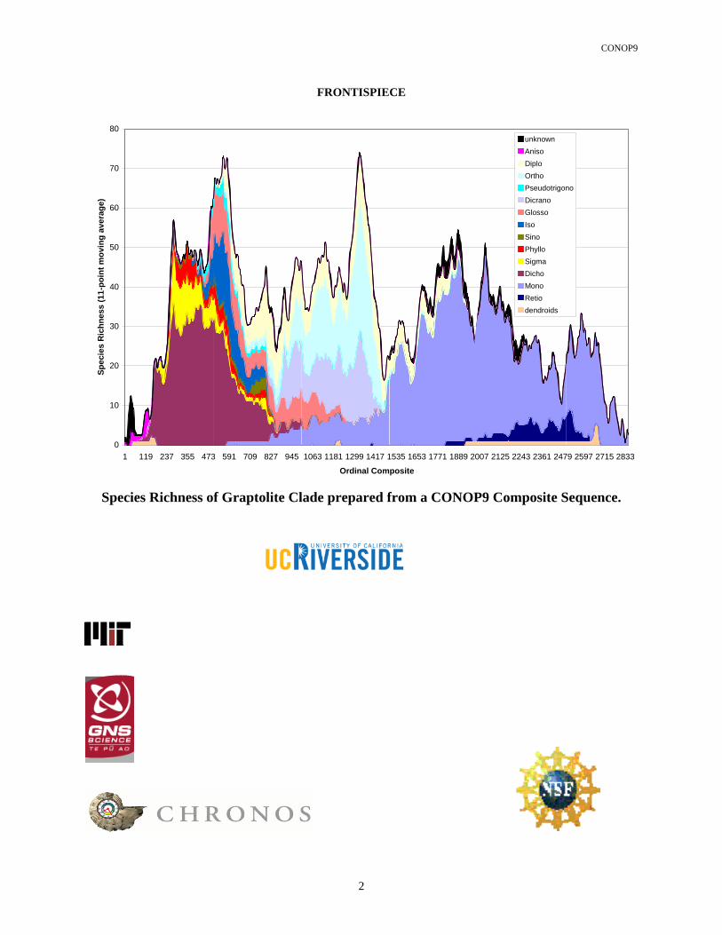
CONOP9

2

FRONTISPIECE

0

10

20

30

40

50

60

70

80

1 119 237 355 473 591 709 827 945 1063 1181 1299 1417 1535 1653 1771 1889 2007 2125 2243 2361 2479 2597 2715 2833

Ordinal Composite

Spec

ies

Ric

hnes

s (1

1-po

int m

ovin

g av

erag

e)

unknownAnisoDiploOrthoPseudotrigonoDicranoGlossoIsoSinoPhylloSigmaDichoMonoRetiodendroids

Species Richness of Graptolite Clade prepared from a CONOP9 Composite Sequence.

CONOP9

3

DISCLAIMER The author develops these programs for his own research needs and intellectual development. They are made available ‘as-is’ purely as a professional courtesy to fellow researchers who wish to examine the author’s solutions or try new applications. The programs are distributed free of charge, but without any legal implication that they will be accurate, correct or suitable to any particular instance of the stratigraphic correlation and seriation problems. The author, developer, and publisher assume no legal responsibility or liability for the consequences of decisions that are based upon the output of the programs, whether these result from the internal algorithms or the settings of parameters that must be adjusted by the user to suit each application. Where results are found suitable for scientific publication, the author requests the courtesy of citation in those publications. This manual is updated, as time permits, but always lags somewhat behind experiences that emerge from the continually on-going augmentation, testing and correcting of the programs. The author makes no representation that any component of the program has been subject to systematic beta-testing on a par with commercial software. While users should not expect anything approaching full technical support, the author will attempt to respond to requests for help and welcomes both suggestions for improvement and notification of errors.

CONOP9

4

ACKNOWLEDGEMENTS Much of the development of these programs was supported by four National Science Foundation Grants to Peter M. Sadler. William Kemple, David Strauss, Chuck Mitchell, Steve Leslie, Scott Samson, Mary Droser, Nigel Hughes, James Valentine, Stan Awramik, Jeff Mount, Philip Signor, and William Zinsmeister were co-PI’s or collaborators in one or more of these grants. Lucy Edwards and Michael Murphy introduced Sadler to graphic correlation. David Strauss recognized that the correlation problem must be tractable. William Kemple established the feasibility of applying simulated annealing to these problems and co-wrote the earliest versions of the program. Robert Dell showed us how to implement reoptimization. Roy Plotnick and Mike Foote shared ideas about using genetic algorithms. John Alroy generously discussed several components of Appearance Event Ordination. Paleontologists at AMOCO, especially Rich Lane and Jeff Stein, generously shared their experiences and practices with automated graphical correlation and encouraged this venture. Sabbatical leaves supported in part by the New Zealand Crown Institute of Geological and Nuclear Sciences and by MIT facilitated critical test projects and provided an ideal environment for developing new code. The NSF CHRONOS initiative implemented CONOP9 as a Web service, with the generous support and expert advice of Cinzia Cervato, Doug Fils, Doug Greer, Josh Reed and Geoff Bohling. Gil Klapper, Roger Cooper, Mike Murphy, Chuck Mitchell, James Crampton, Roderick Brame, Mark Webster, Vladimir Davidov, Bruce Wardlaw, and Bernd Kaufmann furnished unpublished data sets against which the CONOP programs were tested. Questions arising during graduate research by Rosemary Cody (UNL), Carlos Cuartas (Ecopetrol), Yanina Narvez (CICESI), and Jen Sabado (UCR)stimulated several program developments. Roger Cooper, James Crampton, and Marilyn Kooser provided indispensable encouragement and valuable suggestions during development of the CONOP programs. Marilyn Kooser wrote two additional guides to CONOP, one after her experiences as a novice user, the other after drawing range charts with Excel.

CONOP9

5

CONTENTS:

A PRELIMINARIES ...............................................................................................8

A.1 SYSTEM REQUIREMENTS ............................................................................................................................8 A.2 INSTALLATION ...............................................................................................................................................8 A.3 WATCH A SAMPLE RUN ..............................................................................................................................11 A.4 WARNING .......................................................................................................................................................14

B USERS’ GUIDE.................................................................................................15

B.1 THE CORRELATION AND SERIATION PROBLEMS IN A NUTSHELL................................................15 B.2 CONSTRAINED OPTIMIZATION................................................................................................................18

B.2.1 THE CORRELATION PROBLEM...........................................................................................................18 B.2.2 THE SERIATION PROBLEM..................................................................................................................18 B.2.3 DATA AND CONTRADICTIONS...........................................................................................................19 B.2.4 OPTIMIZATION AND REGRESSION....................................................................................................19

B.2.4.1 Two Levels of Optimization ...............................................................................................................20 B.2.5 THE STRATIGRAPHIC “LINE OF CORRELATION” ..........................................................................20

B.2.5.1 Two dimensional form........................................................................................................................20 B.2.5.2 Multidimensional form .......................................................................................................................23 B.2.5.3 Local Stratigraphic Observations as Degrees of Freedom..................................................................23

B.2.6 AN ANALOG for THE COMPLEXITY OF STRATIGRAPHIC OPTIMIZATION...............................24 B.2.7 CONSTRAINTS........................................................................................................................................25 B.2.8 MEASURES OF MISFIT ..........................................................................................................................26

B.2.8.1 Ordinal Misfit......................................................................................................................................26 B.2.8.2 Interval Misfit .....................................................................................................................................26 B.2.8.3 Measures Related to Constraints.........................................................................................................27 B.2.8.4 Relative Size of the Misfit Values ......................................................................................................28 B.2.8.5 No One ‘Right‘ Measure.....................................................................................................................28 B.2.8.6 Negative Evidence ..............................................................................................................................29 B.2.8.7 Mid-Range Events ..............................................................................................................................29 B.2.8.8 Secondary Measures of Misfit ............................................................................................................30

B.2.9 WEIGHTED OBSERVATIONS ..............................................................................................................31 B.2.9.1 Zero Weights.......................................................................................................................................33 B.2.9.2 Objective Weights..............................................................................................................................33

B.2.10 EXCLUSIVE TAXA ..............................................................................................................................34 B.3 SOLUTION STRATEGIES.............................................................................................................................37

B.3.1 Forward Solution .......................................................................................................................................37 B.3.2 Inversion ....................................................................................................................................................37

B.4 EXERCISE ONE: ...........................................................................................................................................38 B.4.1 The Input File Structures ...........................................................................................................................38 B.4.2 The Graphical Output ................................................................................................................................39

B.4.2.1 Taxon Range Charts............................................................................................................................40 B.4.2.2 Collection Quality ...............................................................................................................................40 B.4.2.3 2-D Lines of Correlation.....................................................................................................................41 B.4.2.4 Fence Diagrams ..................................................................................................................................41 B.4.2.5 Section Range Charts ..........................................................................................................................42

B.4.3 The Output Files ........................................................................................................................................44

CONOP9

6

B.4.4 Changing the Constraints ...........................................................................................................................45 B.4.5 Changing the Measure of Misfit ................................................................................................................46 B.4.6 Comparison with Shaw's Solution .............................................................................................................46 B.4.7 Limitations of the Traditional Graphic Method .........................................................................................47 B.4.8 Advantages of the Traditional Graphic Method ........................................................................................48 B.4.9 The Initial Solution ....................................................................................................................................48 B.4.10 HOW TO RECOGNIZE A VERY GOOD Solution ...............................................................................49 B.4.11 A WARNING ABOUT LARGER DATA SETS ....................................................................................50 B.4.12 VARIANTS OF THE RILEY PROBLEM..............................................................................................50

B.5 SIMULATED ANNEALING...........................................................................................................................52 B.5.1 Starting Points for the Search ....................................................................................................................52 B.5.2 A topographic analog for search algorithms ..............................................................................................52 B.5.3 The mineralogical analogy for simulated annealing ..................................................................................53 B.5.4 Different Step Sizes ...................................................................................................................................54 B.5.5 Stringing the Steps Together......................................................................................................................55 B.5.6 Cooling Schedules .....................................................................................................................................55 B.5.7 Running Times...........................................................................................................................................57 B.5.8 Other Cooling Protocols ............................................................................................................................59 B.5.9 PARALLEL Simulated ANNEALING .....................................................................................................59 B.5.10 TWO-STAGE ANNEALING..................................................................................................................59 B.5.11 ADAPTIVE Simulated ANNEALING....................................................................................................60 B.5.12 Simulated Tempering...............................................................................................................................60 B.5.13 The Greedy Algorithm.............................................................................................................................60 B.5.14 Tabu search ..............................................................................................................................................61 B.5.15 Genetic Algorithms..................................................................................................................................61

B.6 EXERCISE TWO:...........................................................................................................................................63 B.6.1 Two Regions with Very Good Fit..............................................................................................................63 B.6.2 The Source of the Ambiguity.....................................................................................................................64 B.6.3 Tuning the Search to the Best Fit...............................................................................................................67

B.7 RELATIONSHIP OF CONOP TO CLADISTICS .........................................................................................70 B.7.1 Missing Questions.....................................................................................................................................70 B.7.2 Separate but Equally Difficult Optimization Tasks ...................................................................................70 B.7.3 Stratigraphic Information in Cladistic Analyses ........................................................................................72 B.7.4 Parallels in the Optimization of Trees and Fences.....................................................................................73 B.7.5 Fundamental Differences Between Trees and Fences................................................................................74 B.7.6 Procedural Possibilities ..............................................................................................................................75

B.7.6.1 Correlation of Character States and Taxa ...........................................................................................75 B.7.6.2 Incorporating Parsimony Trees into Correlation Problems.................................................................75 B.7.6.3 Consensus Sequences from Trees and Fences ....................................................................................75 B.7.6.4 Incorporating Stratigraphic Sequences into Cladistic Analysis ..........................................................76

C SUMMARY of FILES and SYNTAX..............................................................77

C.1 THE CONOP PROGRAM FILES ..................................................................................................................77 C.1.1 CONOP9.CFG ...........................................................................................................................................77 C.1.2 CONOP9.EXE ...........................................................................................................................................77 C.1.3 CONTROL9.EXE......................................................................................................................................77 C.1.4 CONSORT9.EXE ......................................................................................................................................78 C.1.5 CONMAN9.EXE (still preliminary!!) ......................................................................................................78

C.2 BEGINNER's COMMAND SYNTAX.............................................................................................................81 C.3 FULL COMMAND SYNTAX..........................................................................................................................83

C.3.1 Parameters that identify the input data.......................................................................................................83

CONOP9

7

C.3.2 Parameters that alter the best solution........................................................................................................83 C.3.3 Parameters that influence efficiency of search for best solution................................................................83 C.3.4 Parameters that determine the nature and location of output .....................................................................84

C.4 INPUT FILE FORMATS................................................................................................................................85 C.4.1 FORMAT FOR "LOADFILE" and "PREPFILE" .....................................................................................85

C.4.1.1 Sorting.................................................................................................................................................85 C.4.1.2 Record Structure .................................................................................................................................85 C.4.1.3 Event-type Codes ................................................................................................................................87 C.4.1.4 Zero Weights.......................................................................................................................................89 C.4.1.5 Possible Combinations of Type and Move .........................................................................................89 C.4.1.6 Permitted* combinations for paired events in one section..................................................................90 C.4.1.7 Possible treatments of caved ranges (“tops only data”) ......................................................................90 C.4.1.8 Possible treatments of reworked ranges (bases only data)..................................................................91 C.4.1.9 Possible treatments of caved-&-reworked ranges...............................................................................91

C.4.2 FORMAT FOR "SECTFILE"....................................................................................................................91 C.4.2.1 FORMAT FOR "LABELFILE"..........................................................................................................92 C.4.2.2 FORMAT FOR "EVENTFILE" .........................................................................................................92

D COMMAND REFERENCE See Part II ........................................................94

E APPENDICES.....................................................................................................95

E.1 REFERENCES and BIBLIOGRAPHY ..........................................................................................................95

F INDEX .................................................................................................................99

CONOP9 PART B USERS’ GUIDE

8

A PRELIMINARIES

A.1 SYSTEM REQUIREMENTS

CONOP9 has been run successfully on the following operating systems: WINDOWS 95, 98, 2000, NT, XP (also with Windows Emulator on an iMAC)

with the following processors: Intel 386, 486, Celeron, Pentium II-IV and with as little as 32Mb to as much as 1Gb of RAM. The program sets its internal array sizes at run time, according to the size of the input files, i.e. the number of sections and events in the instance of the problem to be solved. Memory, disk storage, and CPU speed influence the running time of the program. Instances that are too big for the available RAM will cause excessive swapping during the run. Instances that are too big for the disk storage may crash when trying to write exhaustive output files. Instances that exceed 260 sections and 1440 taxa would be larger than any that have been tested to date. A few examples have been compiled to run from a CD within a Powerpoint presentation. They do not attempt to write to disk. In general, CONOP9 will NOT run from CD, because the program writes a log file while running.

A.2 INSTALLATION

CONOP files may be supplied on one CD, one ZIP drive, or two to three 3.5inch diskettes. It is recommended that all the supplied files are initially kept in their nested arrangement (if any) and copied into a single folder or sub-directory on a hard drive. If the files have been copied from a CD, it may be necessary to change their attributes from “read-only” to “archive.” The attributes may be seen in Windows Explorer using the “Details” view or by opening “Properties.” Change ‘R’ to ‘A.’ The programs will run from the ZIP drive, but performance will not be optimal. THE PROGRAMS WILL NOT RUN FROM THE CD, because attempts to write reports at run time will fail in this read-only format. They will probably fail during a run from 1.44Mb diskettes because there is too little room for writing run-time files.

To run the program there must be at least one executable file and a configuration file: CONOP9.EXE the main application program CONOP9.CFG run configuration with editing instructions the .CFG file is read by the application prior to every run

Usually there are two or three more executable files: CONSORT9.EXE assists in the preparation of input file; not needed for files prepared

by CONMAN9 CONTROL9.EXE analyzes stratigraphic input file, performing analyses that do not

require solving the correlation/seriation problem CONMAN9.EXE manages range chart data and prepares input files for CONOP9

- preliminary version distributed with CONOP9 version 7.1 (8.18.03) - this program has been subjected to the least amount of testing

Each problem instance requires one master file of input data and may include optional dictionary files that allow the program to report results in terms of taxon and section names rather than numbers:

occurrence data file one line for every observed event (required) section dictionary section names corresponding to numbers in required data file (optional) event dictionary event names corresponding to numbers in required data file (optional) label list stratigraphic labels to attach to event numbers in required data file (optional)

section tags two files to classify the sections e.g. paleolatitude (optional) event tags two files to classify the events e.g. higher taxonomic groupings (optional)

To see examples of the input data files and dictionaries, examine the following files are sample data sets:

CONOP9 PART B USERS’ GUIDE

9

SAMPLE DATA - Riley Formation Trilobites (Cambrian): RILE7x62.DAT occurrence data (62 taxa and 7 sections) RILEY7.SCT section dictionary (optional) RILEY62.EVT event dictionary (optional) RILE7x124.DAT occurrence data – recast as 124 unpaired range-end events RILEY124.EVT recast event dictionary for above RILE7x62x9.DAT occurrence data – modified to illustrate mid-range events and unpaired events RILEY66.EVT modified event dictionary for above

SAMPLE DATA - Mohawk Valley Graptolites (Ordovician): MO6X21X7.DAT occurrence data MOHAWK7.SCT section dictionary (optional) MOHAWK28.EVT event dictionary (optional)

SAMPLE DATA - Liassic Ammonite Genera LIAS7x20.DAT occurrence data LIAS7.SCT section dictionary (optional) LIAS21.EVT event dictionary (optional)

SAMPLE DATA - ODP Cenozoic Microfossils and Magnetostratigraphy (N. Atlantic) ODP20x177x19.DAT occurrence data ODP20.SCT section dictionary (optional) ODP196.EVT event dictionary (optional)

One or more of these sample data sets will probably have been included with the distribution disks. Usually they can be found in individual subdirectories together with executable and configuration files that are ready to “click and run.”

In addition to the notes attached to CONOP9.CFG, instructional materials may be present in the following files (typically in a folder labeled “OTHER.”):

README.TXT Instructions for copying files (Pete Sadler, 1998 - 2003)

MANUAL.DOC Microsoft Word file (Pete Sadler, 1998 - 2003)

MANUAL9.PDF Adobe Acrobat file (Pete Sadler, 1998 - 2003)

CONOP9.DOC Microsoft Word file - obsolete versions (Pete Sadler, 1998 - 2000)

CONOP9.PDF Adobe Acrobat file - obsolete versions (Pete Sadler, 1998 - 2000)

EXCELGUIDE.DOC A quick-start guide to CONOP for users with prior knowledge of biostratigraphy and Excel ( Marilyn Kooser, 2002) QUICKREFERENCE.DOC A one-page summary to accompany the excel-guide ( Marilyn Kooser, 2002) EXCELHRANGECHT.XLS Worksheet to draw range charts in horizontal format ( Marilyn Kooser, 2002) EXCELVRANGECHT.XLS Worksheet to draw range charts in horizontal format ( Marilyn Kooser, 2002) NOVICEGUIDE.DOC A quick-start guide to CONOP for novice users with little prior experience of biostratigraphy and computer programs. (Marilyn Kooser, 2002)

Typical CD organization:

CONOP9 PART B USERS’ GUIDE

10

MAIN folder PROGRAMS folder - 2 to 4 programs as executable files (___.EXE) DOCUMENTATION folder - 1 to 2 manuals as acrobat files (___.PDF) - a blank configuration file (CONOP9.CFG) - 1 to 2 brief extracts of the CONOP9.CFG as text files (___.TXT) OTHER folder DOS folder - source files for an obsolete skeletal DOS version EXCEL_USERS folder - advice on preparing input files with Excel (Microsoft trademark) NOVICE folder - advice first-time users SAMPLE folder each sub folder contains a different data set

CONOP9 PART B USERS’ GUIDE

11

A.3 WATCH A SAMPLE RUN Before reading about the workings of these programs, it may be useful to watch one run. Proceed as follows to run the data set for the Cambrian trilobite faunas of the Riley Formation of Texas. These are the classic Palmer data used by Alan Shaw and Jean Guex to illustrate other correlation methods. In the 1.44Mb diskette format, there is one copy of CONOP9.EXE and it is placed with all the files necessary to run this demonstration; make sure that RILE7x62.DAT is included. In the CD and ZIP formats, there are multiple copies of CONOP9.EXE, each in a subdirectory with different sample data. Find the sub-directory that contains the file RILE7x62.DAT; it is the “standard” Riley example.

1. Copy the whole set of files to a hard disk and cancel any “read-only” attributes. 2. Make sure that the supplied executable file (conop9.exe) and the configuration file (conop9.cfg) are in the

same folder or as any data files and dictionaries . 3. Make sure that Windows9x includes the Times New Roman font or has designated a substitute file for this

font name. 4. Open the configuration file CONOP9.CFG in any word processor or notepad program that can handle a

large ASCII text file. Make sure that the following lines appear as shown

&getinn . . . SECTIONS=7 TAXA=62 EVENTS=0 MAX_LEVELS=150 MAX_LABELS=15 . . .

5. Make sure that following three lines have the right filenames. The example below does not include a path with the file name; it assumes that these three files are in the same folder as CONOP9.EXE and CONOP9.CFG. If you have placed the sample data files elsewhere, edit the portion of each line after the “=” sign to add the correct path for your computer. e.g. =’C:\CONOP\DATA\rile7x62.dat’

LOADFILE = 'rile7x62.dat' . . . SECTFILE = 'riley7.sct' LABELFILE = ‘riley.lbl’ EVENTFILE = 'riley62.evt' . . . /

6. Make sure that any paths in the following lines match real paths on your computer. The files need not exist; they will be written at the end of the run. Edit the portion of each line after the “=” sign if necessary.

. . . CURVFILE='riley.grd' CRV2FILE='\riley.gr2' / . . . &getout . . . UNLOADMAIN='outmain.txt' . . . UNLOADSECT='outsect.txt' . . . UNLOADEVNT='outevnt.txt' . . . RUNLOGFILE='runlog.txt' CULLFILE='cull.txt'

CONOP9 PART B USERS’ GUIDE

12

SOLNLIST='solution.sln' STARTFILE='soln.dat' STEPFILE='stepsoln.txt' BESTARTFILE='bestsoln.txt' COMPOSFILE='cmpst.dat' . . . OBSDFILE='ab.dat' PLCDFILE='albet.dat' EXTNFILE='delta.dat' COEXISTFILE='coex.dat' ORDERFILE='ordr.dat' /

7. Make sure that the following lines appear as shown below in order to set up a reasonable run.

&getans PENALTY='INTERVAL' LETCONTRACT='OFF' USENEGATIVE=’OFF’ NEARENOUGH=1.00 EXCLUSIVES=’OFF’ FORCECOEX='SL' HOMERANGE=’SL’ SMOOTHER=0.00 SQUEEZER=0.00 SHRINKER=0.00 TEASER=0.00 STACKER=’SPAN’ / . . . &getrun SOLVER='ANNEAL' STEPS=500 TRIALS=100 STARTEMP=200 RATIO=0.98 HOODSIZE='big' STARTYPE='RAND' STARTSECT=1 STARTEVENT=0 SHOWMOVIES='CHT' TRAJECTORY='ALL' VIDEOMODE='SVGA' STARTSECT=1 PAUSES='ON' . . .

8. Navigate in Windows Explorer to the folder that contains the executable files and (double) click on CONOP9.EXE to run it. Alternatively, navigate to CONOP9.EXE from the RUN panel in the START menu. The program should report some run parameters and then request that you hit the “Enter” key before presenting an animated range chart. Hit the ‘enter’ key again when requested during the running of the program (active window displays message “Awaiting input . . . “ at base) or when a graphics screen has painted and is still.

NOTE 1: If the parameter PAUSES is not set to ‘ON’ then the program might progress directly to the animated range chart without pausing for the ENTER key. Some settings may cause multiple runs to follow one another without pause! The ‘AUT’ setting, for example, causes the run to proceed in a series of short segments, but the results may be meaningless unless other parameters are adjusted accordingly. Use the File Menu and Exit bar to stop such runs. NOTE 2: If the parameter SHOWMOVIES is not set to ‘CHT’ then the animated range chart may be replaced by some other animation and the program might not proceed to the best solution. The ‘DIV’ setting, for example, animates a diversity (species richness) curve.

CONOP9 PART B USERS’ GUIDE

13

Once started, the .EXE file reads the .CFG file to determine which data files contain the problem instance and how it is to be solved. It reports some of the parameters back to the screen. The .EXE file then reads in the data file(s), reports any anomalies, and reports its progress while building necessary arrays. If no anomalies are found (and the Enter key is struck if requested), the search for the best solution will be tracked as an animated range chart. On this chart, time is plotted on the X-axis from left to right. The time-scale is ordinal: it has one unit for each event (124 for the Riley instance of the problem); and each unit has the same length. The taxon ranges are represented as horizontal white lines stretching from the FAD event (left) to the LAD event (right). The program searches through a large set of hypothetical sequences of events to find the one with that best fits the data. With each new trial sequence, the ranges are adjusted on screen to show the latest sequence, thus the range chart appears to be animated. With custom data sets and a little experience, this animated range chart provides many insights into the progress of the run and guides the setting of search parameters.

When the search is complete, the animation will have drawn red and/or green and/or gray curves from upper-left to lower-right across the screen and a green number will appear low on the y-axis. Most likely, for the Riley instance, this number will be close to 3546; this is the value of the interval misfit for the best-known solution to this instance of the problem. Green square symbols are plotted on screen to indicate the misfit between the model range chart and the field observations every time an improvement is found during the run. A grey symbol is plotted to indicate that the last modification of the model sequence did not make an improvement, but was kept anyway. The green symbols should sweep out a discontinuous concave-upward curve of diminishing returns. The grey symbols should make upward excursions from the line of green boxes. The red curve tracks an internal measure related to the likelihood of keeping a modification that does not make an improvement. The red line should sweep out a concave-upward curve from upper left to lower right; in detail, it is a series of horizontal steps. Once the animation has stopped, strike the enter key to display a range chart for the solution with the best fit. This step is necessary because the last solution examined in the search may not be the best. Starting with version DEC 6.1a, it is possible to “walk” though the ranges in this screen using the <, -, +, and > keys; the active range paints in bright blue and the taxon name is plotted in the left margin. By this time the program has also written text and data files that record the results of the search. For a quicker glimpse of the results several graphical summaries are available.

CONOP9 PART B USERS’ GUIDE

14

9. Strike return once more to move on to the output options. Click on the pull down menu marked “GRAPHICAL OUTPUT.” (In early versions the same options were available under “GRAPHICS OPTIONS.”) Click on any option to examine various aspects of the solution. Use the Esc key to move from screen to screen. Click on the bottom bar to log out of CONOP. The program signs off with a summary of the misfit measures for the best solution and report the duration of the search. The reported duration ignores the time spent entering the data and any time spent examining output graphics.

10. The “SCREEN LIST OUTPUT” and “TEXT-FILE OUTPUT” menus (later versions only) are less

attractive. The SCREEN LIST menu offers a variety of lists of the optimal sequence; the lists become increasingly unwieldy and illegible as the number of events grows. The TEXT FILE menu merely echoes the names of files written to disk.

11. In order to determine what has been going on during the animation of the range chart, read on. There

follows an explanation of the method, keyed to the relevant lines in the .CFG file. These lines from the .CFG file are identified in boxes at strategic places in the text. Read the general introduction to the method. Then the Riley data set can be explored in more detail as an exercise. This data set can be run several times with different settings for those parameters that can influence the nature of the solution. In a later exercise, a poorly behaved data set will be introduced in order to examine the impact of those settings that influence the efficiency of the search heuristics. Appendices at the end of the notes include a full reproduction of the configuration file; it contains extensive explanatory notes on the use of this file. There is also an abbreviated sample of an output text file and a listing of the data files used in the examples.

The basic Riley example is small and simple. It uses 7 sections and 62 taxa. Depending upon hardware and the graphical settings, it should run in less than 1 minute. Custom data sets have been built with over 430 sections and more than 1900 taxa. They take much longer to run -- weeks on old machines! The 62 taxa in the Riley data set are all entered as a paired FAD and LAD; this is the basic event format for which CONOP was originally designed and has been extensively tested. Other types of event are now permitted: one mid-range event per taxon, unpaired appearances and disappearances, dated events, and marker beds. None of these event types has been exposed to the amount of testing that the FAD-LAD pairs enjoy. They are explained below and are included in some of the other sample data sets.

A.4 WARNING

Whether or not the CONOP search ends with a good solution, depends upon user-selected search parameters. Thus, the program aids an expert to solve complex problems. Without some intelligent interaction from users familiar with the stratigraphic data or heuristic searches, the program may terminate too soon, leaving a terrible solution. The larger the data set, the more likely this undesirable outcome.

To avoid these miserable outcomes:

1. Be sure to read more of the manual and wrestle with the MOHAWK sample data before attempting to solve a custom instance of the problem.

2. Always err on the side of inefficiency -- set up a longer slower search than appears to be necessary. Read about the PAUSES=”AUT” option.

3. Try to improve putative solutions by habitually restarting the program from its previous “best solution.” (Look for reference entries under STARTTYPE) Set the search parameters so that the second run accepts a few deleterious mutations before trying to improve upon the last result; i.e. set the restart temperature above the final temperature of the original search. Watch the animation to ensure that the prior solution is sufficiently degraded before improvements are attempted.

CONOP9 PART B USERS’ GUIDE

15

B USERS’ GUIDE B.1 THE CORRELATION AND SERIATION PROBLEMS IN A NUTSHELL

Later sections present formal statements of the stratigraphic problems and a systematic account of CONOP. They are necessarily long-winded. Some readers may prefer to plunge into this brief statement that assumes a working familiarity with biostratigraphic correlation and quantitative stratigraphy. Others will want to skip all the general description and refer directly to the reference section for configuration options. To accommodate as many readers as possible, the manual revels in redundancy between the “nutshell,” “description,” and “reference” portions.

The raw data for correlation and seriation problems are stratigraphic range charts, one for each section in the problem. The charts show the stratigraphic extent of taxon ranges. The problem is to determine the sequence and spacing of the ends of the ranges. The charts may also show the stratigraphic levels of other events to be placed in the sequence: radiometric dates, cycle boundaries, paleomagnetic reversals, tuff beds, etc. It may often be useful to include single fossil collections as a record of taxon coexistences to supplement those seen in range charts; treat them as stratigraphic sections with only one collecting horizon. It is also possible to include pseudo-sections that record superpositional order, but do not have a true thickness scale; in pseudo-sections the units of the superpositional scale may be formations, biozones, or numerical age. If taxa in a pseudo section are combined by zone or formation, coexistence must be established by overlapping ranges, not by mere co-occurrence at a single level; this will be termed using the sensu stricto rule for establishing coexistence, rather than the sensu lato rule. In any case, sensu stricto rules allow for the possibility that the sections contain condensed levels or bulk samples.

The fundamental solutions to the stratigraphic correlation and seriation problems are sequences of ancient events, mostly the originations and extinctions of fossil taxa, that represent their correct historical order, with or without an attempt to scale the intervals between events. The solutions may be represented as fence diagrams and time-scales respectively. Both may be recast as diversity curves that plot taxon-richness as a function of time. Other derivative products include time series of taxon longevity, extinction rate, etc. All results require finding the composite range chart that best combines all the local stratigraphic observations. The local stratigraphic sections are arrayed as parallel fence posts and/or stacked in series according to the time intervals that they span. The difference between correlation and seriation is one of degrees -- the degree to which pairs of stratigraphic sections do (correlation) or do not (seriation) overlap in the time intervals that they span.

The problems are difficult because local stratigraphic sections underestimate the true taxon ranges and contradict one another in detail concerning the sequence of stratigraphic events. The quality of solutions cannot be measured against the truth; in practice, the truth is never known in detail. The relative merits of solutions must be measured in terms of their fit to the data.

With severe simplifying assumptions, solutions can be built from the observed data either systematically and slowly by hand (Shaw’s method) or rapidly by computer (RASC method). The computer methods are preferable because they force all subjective judgments to be made explicitly and in advance; their results are reproducible.

The CONOP program minimizes the simplifying assumptions and maximizes the flexibility of the choice of measures of fit between solutions and the data. This is achieved by inverting the solution process. Instead of building a solution from the data, CONOP works through a series of iteratively improved guesses about the solution. Each guess is compared with the data; the misfit between the solution and data guides the next guess. Geophysicists like to call the process “inversion.” Others may notice elements of Bayesian logic -- modify prior notions about the solution by reference to the data.

Seriation problems require more complex measures of misfit than correlation problems. They must consider negative evidence in order to stack the sections correctly. As a result, searches for the solution of seriation problems tend to take more time and are more difficult to tune.

The stratigraphic correlation problem is “Non-Deterministic Polynomial-Time Complete” (Dell et al. 1992). In other words, the time it would take to work through all possible solutions increases exponentially (or worse!) as the size of the data set increases. The size of the data set is the number of taxa and the number of sections. The product

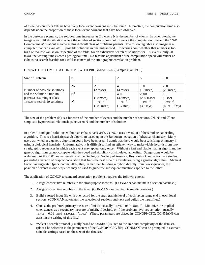
CONOP9 PART B USERS’ GUIDE

16

of these two numbers tells us how many local event horizons must be found. In practice, the computation time also depends upon the proportion of these local event horizons that have been observed.

In the best-case scenario, the solution time increases as 2N, where N is the number of events. In other words, we imagine an unlikely situation where the number of sections does not influence the computation time and the “N-P Completeness” is about as tame as this difficult class of problems permits. The following table also imagines a computer that can evaluate 10 possible solutions in one millisecond. Concerns about whether that number is too high or too low vanish on inspection of the table: for an exhaustive search of solutions for 100 events (only 50 taxa), the waiting time exceeds geological time. No feasible adjustment of the computation speed will render an exhaustive search feasible for useful instances of the stratigraphic correlation problem.

GROWTH OF COMPUTATION TIME WITH PROBLEM SIZE (Kemple et al. 1995) Size of Problem

N 10 20 50 100

2N

20 (2 msec)

40 (4 msec)

100 (10 msec)

200 (20 msec)

N2

100 (10 msec)

400 (40 msec)

2500 (250 msec)

104

(1 sec)

Number of possible solutions and the Solution Time (in parens.) assuming it takes 1msec to search 10 solutions 2N

1.0x103

(100 msec) 1.0x106

(1.7 min) 1.1x1015

(3.6 Kyr) 1.3x1030

(4.0x1012Myr)

The size of the problem (N) is a function of the number of events and the number of sections. 2N, N2 and 2N are simplistic hypothetical relationships between N and the number of solutions.

In order to find good solutions without an exhaustive search, CONOP uses a version of the simulated annealing algorithm. This is a heuristic search algorithm based upon the Boltzmann equation of physical chemistry. Many users ask whether a genetic algorithm could have been used. I admit that there would be a satisfying symmetry in using a biological heuristic. Unfortunately, it is difficult to find an efficient way to make viable hybrids from two stratigraphic sequences in which each event may appear only once. Without a fast and viable mating algorithm, the genetic algorithm cannot compete with the speed and simplicity of simulated annealing. Suggestions would be welcome. At the 2001 annual meeting of the Geological Society of America, Roy Plotnick and a graduate student presented a version of graphic correlation that finds the best Line of Correlation using a genetic algorithm. Michael Foote has suggested (pers. comm. 2002) that, rather than building a hybrid directly from two sequences, the position of events in one sequence may be used to guide the subsequent mutations applied to the other.

The application of CONOP to standard correlation problems requires the following steps:

1. Assign consecutive numbers to the stratigraphic sections. (CONMAN can maintain a section database.)

2. Assign consecutive numbers to the taxa. (CONMAN can maintain taxon dictionaries.)

3. Build a sorted input file with one record for the stratigraphic level of each taxon range end in each local section. (CONMAN automates the selection of sections and taxa and builds the input files.)

4. Choose the preferred primary measure of misfit (usually ‘LEVEL’ or ‘SEQUEL’). Minimize the implied coexistences as a secondary measure of misfit, if desired, or if the problem involves seriation (usually TEASER=0.01 and STACKER='COEX' . (These parameters are placed in CONOP9.CFG; CONMAN9 can assist in the writing of this file.)

5. *Select a search protocol (usually based on ‘ANNEAL’) suited to the size and complexity of the data set. (place t he selection in the parameters of the CONOP9.CFG file; CONMAN9 can be prompted to estimate suitable settings based on the size of the data set.)

CONOP9 PART B USERS’ GUIDE

17

6. Run the primary search. The purpose is to find a sequence of events to which all the local sections can be fit with a minimum of adjustments; i.e. minimize the implied short-comings of the observed fossil record.

7. *Extend the search (restart from the current best solution) until no further improvement is achieved.

8. *Repeat the search (perhaps with different search protocols) until satisfied that the results are stable. The purpose is ensure that the search is not “trapped” in a local minimum.

9. *Run short secondary searches to minimize any secondary measure of misfit (usually ‘STEAL’) while holding the primary measure to the previously determined minimum, or better. The purpose is to tease apart any arbitrarily interleaved associations of taxa and to shorten any needlessly long taxon ranges.

10. Examine the details of the solution onscreen and in the text files.

11. *Initiate a series of sub-optimal searches around the first solution that will map out the best-fit intervals and relaxed-fit curves for all the events. The object is to find all the equally well-fit solutions, examine some nearly best-fit solutions, and build a set of confidence intervals.

* REMEMBER, These programs are tools that aid an expert to search for and recognize good solutions to

intrinsically complex problems for which unique true solutions are not knowable. Flawed data or poorly adjusted searches upon good data sets may lead to very bad solutions.

“Garbage-in – garbage-out” (the stratigraphic data should be good) “Garbage-settings – garbage-out” (the optimization criteria must be appropriate) BE WARNED, These programs can digest large volumes of information, but it takes a much larger volume of

data to report all the insights and analyses “Mole-hills-in – mountains out” (time saved calculating becomes time spent reading) Typical instances of the correlation and seriation problems are underdetermined. That is, there is insufficient information to determine a unique correct solution. A good analysis explores the range of equally good solutions and examines the sources of mis-fit in order to identify weaknesses in the raw data. If the optimization criteria are sound, “ bad” solutions (the nature of the output garbage) can be used to track down bad data. The total misfit between a solution and the raw data can be viewed in all its incremental parts to determine which events in which sections contribute the greatest misfit. Such exploration of the data may, perhaps, be more important than any one solution.

CONOP9 PART B USERS’ GUIDE

18

B.2 CONSTRAINED OPTIMIZATION

[Extended version of Kemple et al., 1995] Any account of the CONOP programs should begin with a formal statement of the stratigraphic correlation and seriation problems. Otherwise, any discussion of solution strategies would be premature. The nature of the solution and the data dictate that the problem is a constrained optimization and, therefore, shares many fundamental properties and prerequisites with the much more familiar exercise of linear regression. Because the correlation problem is far more complex than linear regression, however, solution strategies emerge by comparison with the classic traveling salesman problem (TSP) of operations research. The TSP is a challenge to find the shortest or least expensive route for a salesman who must visit a large set of cities. The formula for the distance or cost that is to be minimized is variously known as the “objective function,” the “cost,” or the “penalty.”

B.2.1 THE CORRELATION PROBLEM The stratigraphic correlation problem concerns the sequence and spacing of prehistoric events such as the appearance and disappearance of fossil taxa, changes in rock chemistry and remanent magnetization, volcanic ash falls, etc. A solution for the problem entails three conceptually straightforward tasks:

i. The sequencing task: arrange the set of ancient events in their correct sequence in time. ii. The spacing task: determine the spacing between these events, also on a time scale. iii. The locating task: locate horizons in all the local stratigraphic sections that correspond in age with

each of the events; this task involves a set of local thickness scales.

The sequencing task is prerequisite for the other two tasks. The locating task and the spacing task may be attempted separately, once the sequence has been determined. The sequencing and locating tasks may be completed using only the local biostratigraphic observations because these two tasks do not involve a time scale. The spacing task cannot be attempted without additional data or assumptions concerning the relationship of the local thickness scales to time. Thus, there are practical and theoretical reasons for separating the spacing task from the other two. The RASC (Gradstein et al., 1985; Agterberg, 1985, 1990) method achieves this separation; traditional graphic correlation (Shaw, 1964; Miller, 1977) does not.

B.2.2 THE SERIATION PROBLEM Building geologic time scales is a seriation problem. The seriation problem involves the same three tasks as the correlation problem. The difference lies in the time span of the individual stratigraphic sections relative to the time span of the whole sequence of events. In the standard correlation problem, the individual sections are approximately contemporaneous and span most or all of the sequence of events; for most pairs of sections, the time interval of their overlap is a substantial fraction of the time spans of both sections. In a seriation problem the sections are very short relative to the time span of the whole sequence of events; many pairs of sections in a seriation problem do not overlap in age. In other words, the solution of a correlation problem arranges most of the sections in parallel; the solution of a seriation problem must stack some sections in series. It emerges that seriation problems require attention to negative evidence -- missing taxa. Correlation problems can, and should, be solved using positive evidence alone. The computer has difficulty distinguishing a true seriation problem from the provinciality problem. Provinciality of faunas may cause sections that do overlap in time to have no taxa in common. Strategies for solving seriation problems must not be too aggressive, otherwise they make nonsense of provinciality. The user must be sensitive to this issue on an ad-hoc basis and take care to include sufficient cosmopolitan taxa or other events that can tie together the faunal provinces. In other words, the positive evidence that stratigraphers use to prove coeval provinces should not be denied to the computer. It is often critical, however, to weight the long-ranging cosmopolitan taxa low relative to other taxa, especially when the taxon duration spans a longer interval than most stratigraphic sections. The differential weighting is most critical when the preservation of the long-ranging cosmopolitan taxa is rather patchy. Instead of ranging through most sections in which they occur, they are typically found as incomplete ranges that appear not to extend beyond many sections. The computer algorithms will tend to equate all these partial ranges and, inappropriately condense the local histories. Low weights, prefer solutions that preferentially extend the observed ranges of the long-ranging cosmopolitan taxa.

CONOP9 PART B USERS’ GUIDE

19

How might such a situation arise in practice? Consider the Ordovician conodonts: most taxa appear to be confined to latitudinal provinces in shallow-marine settings; the longer ranging, more nearly cosmopolitan taxa appear to live in basinal settings; they can be preserved with shelf faunas, and basinal strata may be intercalated into shallower water sections, but rather sporadically. The difficult task is to recognize the long-ranging, cosmopolitan taxa, objectively. Can this task be automated? One approach is to assume that the long-ranging taxa will coexist with the largest numbers of other taxa. The fewest coexistences are likely to recorded for short-lived provincial taxa, the most by long-lived cosmopolitan taxa. Of course, these expectations may be confounded by uneven sampling. It is NOT a good strategy to weight taxa inversely according to the number of their observed coexistences: this robs the optimization algorithm of the very differences that it needs to solve the problem. It is often an effective practice to apply low weights to a few taxa with the highest coexistence count. It may be useful to examine a histogram of coexistence counts to identify the outliers that are candidates for low weighting.

B.2.3 DATA AND CONTRADICTIONS The raw data for the correlation and seriation problems are the relative positions of locally observed horizons that record the ancient events in discrete stratigraphic sections. Because of the vagaries of preservation and collection, the local stratigraphic sections typically preserve incomplete sub-sets of the events that occurred in the time interval during which they accumulated. And they tend to contradict one another in detail concerning the sequence of these events. Locally observed ranges of fossil taxa in particular, which are often the most readily available data for correlation, tend to underestimate the true temporal ranges of the corresponding living organisms. The locally observed event horizons may, therefore, differ from the expected or ‘true’ event horizons, and the expected ranges are most often longer than the observed ranges (Edwards, 1982).

Contradictions between the local stratigraphic sections can render the correlation problem extremely difficult. Most practical instances of the problem include so many degrees of freedom and so much contradictory data that the true solution is quite evidently not knowable. Instead, stratigraphic correlation must seek the solution that best fits the local observations and thus minimizes the implied failings of the local stratigraphic records. Notice that artificial data sets which degrade a “known truth” do not, therefore, provide a fully legitimate test of quantitative correlation techniques. Two serious concerns emerge:

1. Unless the artificial degradations properly match the real range and proportions of factors that degrade the fossil record, the tests may be misleading.

2. This kind of test tend to prefer solutions that extend fossil ranges beyond what is required by the observed data and their internal contradictions. In other words, non-parsimonious solutions are preferred. Should the observations set the standard, or a model of putative infidelity of the stratigraphic record? The best answer is that the solution should be true to the data and models of infidelity can be used to make confidence statements about the solution.

B.2.4 OPTIMIZATION AND REGRESSION The familiar method of linear regression is a simpler, but comparable, situation in which we judge a solution by its fit to the data rather than its relationship to some “truth.” Prior to performing a linear regression two critical decisions are made concerning the shape of the solution and the definition of best fit. We decide in advance that the solution is linear and we select one of several possible measures (Macleod and Sadler, 1995) of the misfit between the data points and the regression line. Then, linear regression uses this measure to optimize the fit (minimize the misfit) between the data points and the line, subject to the constraint that the line must be straight. Compared with the two prior decisions, selecting a method of actually finding the best line is rather trivial -- a matter of computational efficiency. To ignore the decisions concerning the form of the line and the measure of misfit is to fail to appreciate that there are other legitimate solutions to the same problem.

Stratigraphic correlation is also a constrained optimization. The misfit between the local data and the expected global sequence of events is minimized, subject to several constraints. Some constraints are mandatory to achieve a feasible answer; others are optional. As in linear regression, the solution will likely change with the choice of constraints and the measures of misfit. The method of optimization, which is the focus of a large body of stratigraphic literature, is really less significant than the two choices that precede it.

CONOP9 PART B USERS’ GUIDE

20

When undertaking a linear regression, the user might decide to examine the results of several measures of misfit and different transformations of the raw data. In effect, this approach uses regression as a tool to explore the nature of the data rather than as a “black box” that offers only one answer. Stratigraphic correlation should surely be approached this way. The CONOP configuration files allow a variety of measures of misfit to be used.

PENALTY='INTERVAL' | ’LEVEL’ | ’EVENTUAL’ | ’ORDINAL’ | ’SPATIAL’ | ’RASCAL’ | ’SEQUEL’ | ‘ROYAL’

B.2.4.1 TWO LEVELS OF OPTIMIZATION If there are I taxa, each possible solution of the correlation problem is both an arrangement of 2I origination and extinction events on a time scale and a placement of the corresponding 2IxJ event horizons in the J local stratigraphic sections. For this reason, the stratigraphic optimization in CONOP must minimize the misfit at two nested levels. The outer level searches for the best global sequence of the 2I origination and extinction events (sequencing task). The inner level searches for the best local placements of the 2I event horizons in each of the J sections (locating task) for any given global sequence. The outer level considers the sum of all the misfits determined by the inner level. The outer minimization routine permutes the supposed order of events and remembers the sequence for which the inner minimization returns the lowest total penalty. It generates a series of sequences, eliminates any that fail to meet all known constraints about the true sequence, and passes the others in turn to the inner minimization routine, which returns the lowest penalty for that solution. The inner minimization works with a local measurement scale, such as stratigraphic thickness or numbers of sampled levels, to determine penalties. It adjusts the position of expected event horizons - horizons that will be assumed to correspond to the "true" age of each event. The purpose of these adjustments is to find the placements that: (1) remain consistent with the arrangement of events that is currently selected by the outer minimization, (2) honor any constraints against range contractions, and (3) yield the lowest total penalty. Not all measures of misfit between the data and the solutions use the inner optimization. Those that do not involve the locating task may bypass the inner optimization. They are measures that sum the disagreements between a sequence and each locally observed order of events; they do not consider the taxon range extensions necessary to make the local sections fit the global sequence. There are several such measures; some consider the pairwise ordering of events as observed and in any hypothetical solution; another consider the difference between the observed coexistences and the coexistences implied by the hypothetical solution; still another compares all the last occurrences, observed and implied above the first occurrence of each taxon. For all these measures of misfit, it is possible to determine, at each hypothetical solution in the search, how the observed ranges will actually be modified to match the current solution. This is not necessary in order to reach a solution; it slows the search considerably; and the inner optimization need not be undertaken until a best sequence has been found by the outer optimization. Note that when both alternatives are available – optimizing only the sequence or actually finding the best adjustments step-by-step – they do not necessarily yield exactly the same answer or the same final misfit value. B.2.5 THE STRATIGRAPHIC “LINE OF CORRELATION” B.2.5.1 TWO DIMENSIONAL FORM If we draw two measured sections as orthogonal axes on an x-y graph, with their bases meeting at an arbitrary origin, then correlations can be shown by points on the graph. The x and y coordinates of these points represent the distances from the origin to two horizons, one in each section, that formed at the same time. Because the layers of rock are laid down younger upon older, the points for all the coeval horizon pairs must form a line whose slope is always non-negative (0 to +90 degrees). Although in some instances the true correlation may be a straight line, the general solution of the stratigraphic correlation problem in this framework is a monotone, non-decreasing, two-dimensional, serpentine curve or "snake." Let’s reserve the term snake as shorthand for the true solution to a correlation problem, leaving the term line of correlation (LOC) to describe any plausible approximation of the true solution, following the common practice started by Shaw (1964).

CONOP9 PART B USERS’ GUIDE

21

SECT

ION

Y

? ?

??

SECTION X

LOC

"snake"

taxon a

taxon

a

The example above plots the range-end coordinates for a single taxon, a, observed in two sections, x and y. The range-end coordinates are shown as the corners of gray boxes. The boxes acknowledge that the observed ranges are minimum estimates for the true range. The snake might not pass exactly through the box corners but must pass through the boxes.

Segments of the snake that are perpendicular to one axis of the plot point to hiatuses in the section plotted on that axis. Time intervals that are represented by hiatus in both sections have no part in the snake, of course. Differences in the ratio of accumulation rate between the two sections cause changes in the positive slope of the snake. Like the snake, LOCs may be curved, segmented, or straight, provided their slope is everywhere non-negative. Selection of a relatively straight LOC corresponds to a judgment that there is little variation with time in the ratio of accumulation rates in the two sections. As increasing numbers of taxa are added to a graphic plot it is less likely that the LOC will be able to pass through all their coordinate points because to do so would require a negatively sloping segment. Points that lie off the LOC contribute an increment of misfit. The size of the increment of misfit may be determined by the distance from the point to the LOC. In the diagram below, the top of the range of taxon b is adjusted upward in section y. Why is this the obvious point to adjust? Section X proves that taxon b should coexist with taxa a and b; these observed coexistences are constraints that section Y must be adjusted to honor. The alternative to extending taxon b upward would be to extend both taxon a and taxon c downward in section Y and taxon c upward in section X -- a greater net adjustment (misfit). Notice how simple stratigraphic logic is guiding the placement of the piecewise linear LOC in a fashion that is more sophisticated than normal linear regression. The levels of gray shading in the diagram attempt to show how the addition of more taxa may identify regions of the plot through which the LOC may satisfy multiple coordinate boxes.

CONOP9 PART B USERS’ GUIDE

22

SECT

ION

Y

SECTION X

LOC

"snake"

taxon a

taxo

n a

taxon b

taxo

n b

Missfit

taxo

n c

taxon c

taxo

n d

taxon d

Events recorded in only one section may be projected into the other using the LOC to create a composite section. The composite section records on one axis an arrangement of all events that is consistent with the observations in both sections. The compositing process allows additional sections to be correlated without using more than two axes, an important consideration for manual correlation. But the LOCs remain two dimensional.

SECT

ION

Y

SECTION X

"snake"

taxon a

taxon

a

older date

youn

ger

date

SECT

ION

Y

SECTION X

"snake"

taxon a

taxo

n a

older

dat

e

younger date

The examples above show the graphic correlation of radiometrically dated horizons which are not from the same marker bed. In combination, they define an area through which the snake may not pass; otherwise the dates would project from one section to the other in false superposition! Unlike taxon range ends, the dated event horizons are not free to be moved in the local sections. Two-dimensional graphic correlation is a wonderful way to discover the rules of stratigraphic constraint and optimization. The real problem is multidimensional, of course. To solve it via a series of 2-D partial solutions requires special measures to satisfy the multidimensional interaction of misfit choices.

CONOP9 PART B USERS’ GUIDE

23

It is not enough to add each section in turn to a growing composite. Such “rounds” must be repeated many times, removing one section each time until there are no more meaningful adjustments to the LOC (Shaw, 1964).

B.2.5.2 MULTIDIMENSIONAL FORM The snake concept extends easily beyond two dimensions. The Deep Sea Drilling Project popularized two-dimensional plots of one section against a time scale. Adding a time scale to the graph of two sections still yields a monotone non-decreasing snake, but in three dimensions. Points on the snake now have coordinates x, y, and time. A plot of J sections gives a snake in J dimensions and the addition of a time scale produces a J+1-dimensional snake. So the fullest solution for a time correlation problem is a J-snake together with the ages of all points on the snake. Shaw (1964) stressed that equivalence in age can be represented without reference to an annual scale of absolute time. Thus, the essential practical problem for graphic correlation is to find LOCs that are good approximations of the J-snake. Because the snake is unknowable, "good" LOCs cannot be defined relative to the snake. Instead, they must be recognized by their relationship to the local stratigraphic observations.

LOC now stands for any possible approximation of a J-snake. The J-dimensional LOC is the solution to the correlation problem. There is no composite section because there is no need to keep a memory of the progress of partial correlations. The J-dimensional LOC is completely described by a matrix in which rows are events and columns are local sections. Rows arranged in the estimated order of events complete the sequencing task. Entries in the matrix cells record the estimated level of the corresponding event horizons; they complete the locating and spacing tasks. Hypothetical composite sections might be created by using the average or maximum spacing of events across all local sections or by combining portions of the local sections that have the same sedimentary facies, but none of this is necessary. In the multidimensional form, we can no longer graphically visualize the placement of the LOC. This has advantages: the LOC must be understood more rigorously as a solution to the three tasks of the correlation problem -- sequencing, spacing, and locating. As explained above, the indispensable task is sequencing. Thus, the essence of act of placing the LOC is to choose a sequence for all the stratigraphic events.

B.2.5.3 LOCAL STRATIGRAPHIC OBSERVATIONS AS DEGREES OF FREEDOM On a two-dimensional correlation graph, events that can be observed in both sections plot as points or rectangular boxes. The snake and all plausible LOCs must pass through these points or boxes. Boxes acknowledge better than points that the location of event horizons has variable precision in practice. They may be regarded as uncertainty boxes for the field observations. They represent degrees of freedom in placement of the LOC or, in the best multidimensional idiom, degrees of freedom in the sequencing of events. The stratigraphic position of a thin, unique ash layer preserved in both sections must plot as a point. The positions of the layer in the sections is not equivocal; there is no freedom to adjust them; the LOC must pass through the observed The LOC most effectively constrained by such chronostratigraphic marker beds. A paleomagnetic reversal would plot as a box: the sides of the rectangle scaled by the sample spacing because a reversal lies between samples, not at a sample. The reversal is free to change positions in sequence with any events that are represented by overlapping boxes or points within the box

Two horizons of known but different absolute age, one in each section, define a no-go region that the snake cannot enter. Two orthogonal lines, drawn at the elevations of the dated horizon, divide the graph into four fields. One of these fields is closed to the snake and all feasible LOCs: nothing below the older horizon may map into other section its (younger) dated horizon. Again, this is the graphical equivalent of a stratigraphic sequence constraint. A feasible solution must place events of known age in their chronological order. In order to constrain the LOC, it is not necessary for dated events to be preserved in more than one section, only that the problem contain at least two of different age.

In typical instances of the correlation problem, most of the available data are local lowest and highest finds of fossil taxa. The lowest finds tend to occur too high in the section and the last finds too low, when compared to the horizons that correspond to either global evolution and extinction events or local immigration and emigration events. Each event should plot as a box; but the extent of the misfit is not evident at the local sections and the rectangle cannot be scaled. Consequently, a taxon range observed in both sections gives only one corner each for the rectangles that contains the true time of first and last appearance. First and last occurrences fix different corners

CONOP9 PART B USERS’ GUIDE

24

of their respective error boxes: the upper right corner for first occurrences and the lower left for last occurrences. These corner points cannot all be expected to lie on the snake and need not lie on the best LOC. In multidimensional form, this means that first occurrences may be adjusted down-section without bound and last occurrences may be adjusted up-section without bound.

An LOC which passes as close as possible to as many of the corner points as possible implies the best overall quality in the local stratigraphic records. It requires the minimum net range extension to make all the local range charts fit one sequence and spacing of events. Shaw (1964, p. 254-257) called this "economy of fit" and established that the best solution in a graphic correlation is the one that realizes the greatest economy of fit. Such a solution is desirable because it is geologically simple. An extreme example shows that this is an almost intuitive line of reasoning. We all quickly reject the hypothesis that all taxa have been in existence since the beginning and none are extinct. The argument is not that the fossil record absolutely refutes such an interpretation; it does not. The hypothesis is rejected because it implies outrageously large and systematic failures of the preservation or collection of fossils. In a way that we must later quantify precisely, the goodness of fit between LOCs and local stratigraphic observations can be measured by the sum of the stratigraphic distances by which the LOC misses the corner points. The scale on which these distances are to be measured is obviously one factor awaiting precise definition.

LOCs need not distribute the correction of local observations equally among all taxa or equally between both sections. Shaw (1964, p. 257) sought the LOC "that results in the smallest net disruption of the best established ranges." He did not weight all taxa equally when assessing the economy of fit. Some combinations of organism and sedimentary facies have higher preservation potential than others; they lead to a higher frequency of fossiliferous levels within the range and are likely to record the local taxon ranges more reliably. Such corner points may be expected to lie closer to the snake and so Shaw weighted the distance by which they misfit the LOC more heavily when assessing the economy of fit. If an LOC can be drawn that lies above all first occurrence corners and below all last occurrence corners, it forces all the range adjustments into the section on the x-axis. Thus, the position of the LOC can also be guided by judgments about the relative suitability of the sections for correlation purposes.

If most of the locally observed taxon range ends are reasonably close to their true positions, then the feasible LOCs may be usefully constrained as the number of rectangle corners increases, even though the individual observations provide little constraint by themselves. Kemple et al (1995) surmise, on the basis of anecdotal and unsystematic experience, that the choice of LOCs will narrow as more taxon ranges are added and that economy of fit will favor LOCs close to the snake. Be warned, however, that facies differences cause some two dimensional plots to be appallingly scattered and render some facies-fossils deleterious for correlation (Sadler and Kemple, 1995).

The task of fitting the most economical LOC to the corners, rectangles and points has clearly emerged as an optimization problem. More precisely, it is a constrained optimization because some LOC placements are geologically impossible. But it is not an instance of optimization that is necessarily best solved by simple linear regression using the method of least squares (Miller, 1977). B.2.6 AN ANALOG FOR THE COMPLEXITY OF STRATIGRAPHIC OPTIMIZATION

RANKING AQUEDUCT PROPOSALS - To appreciate the full scope of the task of ranking different LOCs, imagine the task of finding the best route for an aqueduct (LOC) that will be the nearest source of water for many villages scattered across an uneven landscape. The parable illustrates a range of options for ranking aqueduct routes that is comparable to the choices available to determine economy of fit.

To model the special treatment of local range ends (box corners), imagine that the villagers do not necessarily haul water from the point on the aqueduct closest to their village; instead, their haul roads are required to remain in fields that belong to the village. To maintain water flow, no part of the aqueduct can be routed uphill (non-negative LOC slope). This makes it impossible to route the aqueduct through every village because some occupy hilltops and others lie in closed depressions (equivalent to the problem of contradictory local sequences of highest and lowest finds).

CONOP9 PART B USERS’ GUIDE

25

In the terms of this aqueduct parable, economy of fit ranks possible aqueduct routes by the total distance that remains for villagers to haul water. Compared with a straight route (linear regression or Shaw’s method), the residual haul distance can be significantly reduced by permitting an aqueduct with more than one linear segment.. Because the optimal piecewise-linear aqueduct would be longer than the optimal straight aqueduct, we might pay extra for changes in direction. We might add the raw length of the aqueduct to the total haul distance when ranking different plans; or we could multiply the raw length by a scaling factor that adjusts the balance between local hauling convenience (local stratigraphic observations) and the cost of aqueduct construction (assumptions about accumulation rate).

To prepare for some later sections, notice several other options in the parable. If we weight aqueduct length more heavily than haul distance, we encourage straighter routes without completely prohibiting bends. An absolute constraint against bends can be regarded as the extreme end-member of a set of increasing weights. We can regard some villages as more important, perhaps because of their size and voting habits, and weight their haul distances more heavily. And distance is not the only measurement scale; in this parable, money or votes might be used.

B.2.7 CONSTRAINTS The solution to the sequencing task must satisfy one obvious mandatory constraint: the first occurrence of any taxon must precede its last occurrence. Two factors ensure compliance with this constraint. First, the generation of hypothetical sequences can be forced to honor this constraint. Second, because first occurrences are not free to move up-section and last occurrences are not free to be adjusted down-section, there is no scope for reversing the observed order in any section. Why retain the redundancy? It is always more efficient to be able to prohibit a hypothetical sequence without reference to the local sections; this is achieved by the first factor. Yet the restrictions on the adjustment of range ends are needed to sequence different taxa relative to one another; only the second factor achieves this. Taxa that can be proved to have co-existed in any of the local sections must have overlapping ranges in the true sequence of events. Guex (1977), Rubel (1978), and Alroy (1993) have developed correlation techniques that are built almost exclusively upon this rule. Notice that the nature of the proof of coexistence is open to interpretation. Therefore, the .CFG file offers three possibilities for this constraint. In the strictest sense (‘SS’), only overlapping ranges prove coexistence, i.e. the first occurrence of one taxon lies within the range of the other. Where two taxa merely coexist at one collection level (the first appearance of one taxon lies in the same sample as the last appearance of the other), the apparent coexistence may be an artifact of time-averaging. A looser kind of proof (‘SL’) accepts even this evidence.

FORCECOEX='SL' | ‘SS’ | ‘OFF’|’FILE’

Even when the coexistence constraint is removed, most observed coexistences will be retained in the solution because ranges cannot contract. Nevertheless, applying the constraint makes several differences: 1) it speeds the search by allowing some solutions to be rejected without the calculation of a penalty; 2) it is possible to enforce the interpretation that a single shared horizon is proof of coexistence for a pair of taxa; and 3) it allows hypothetical coexistences to be enforced from a user-supplied file. Because ranges cannot contract, the true level a First Appearance must be below any Last Appearance that has been observed higher in the same section. These pairwise relationships can be enforced as constraints in order to speed the search. They also provide polarity when the misfit is measured solely by implied coexistences.

FORCEFb4L='ON' | ‘OFF’ The locating task may be constrained in its freedom to adjust the local ranges so that they fit the global sequence. It is a mandatory constraint that all sections record the same sequence -- time is unidirectional. If it is assumed that the locally observed ranges under-estimate the true global duration of taxa, then the locating task may extend the observed ranges, but is constrained not to contract them.

LETCONTRACT='OFF' | ‘ON’

Constraints against range contraction forbid the interpretation that fossils have been reworked into younger sediments or carried to anomalously deep levels by drilling operations (Jones, 1958; Wilson, 1964; Foster, 1966). This extreme constraint may be relaxed a little if it is transferred to the measure of misfit. A hypothetical sequence of events that violates a constraint might be considered to cause an infinitely large misfit, thus guaranteeing that all

CONOP9 PART B USERS’ GUIDE

26

geologically feasible sequences will have a smaller misfit and be preferable. This point of view admits the option of making range contractions carry a very large but not infinite misfit. The optimization then discriminates against sequences that require range contractions, but does not prohibit them altogether.

B.2.8 MEASURES OF MISFIT In order to make the taxon range chart for every local sedimentary section fit the same global sequence of events, some of the locally observed range ends must be moved to different positions. This can be achieved in practice by extending some local ranges beyond the observed limits until their ends match the global sequence, i.e. assume that these locally observed ranges underestimate the true ranges. If caving and reworking are believed to have significantly exaggerated the local ranges, it is permissible to shorten the observed ranges in order to fit the global sequence. But the vagaries of migration, preservation, and collection, which shorten the local ranges, are likely to be the prevalent sources of misfit. Regardless of the rules for range contractions, the preceding statements have already identified two distinct measures of misfit: one would compile all the local discrepancies in the order of events; and the other would total all the range adjustment intervals.

B.2.8.1 ORDINAL MISFIT The larger the number of local range ends that need to be moved to a new position, the greater the misfit between the order of events preserved in the local sequences and the global solution. The corresponding optimal solution would be the one that least contradicts the locally observed sequences of pairs of events. A measure of misfit based upon pairwise contradictions drove Hay’s (1972) solution of the correlation problem and is the basis of the RASC program (Agterberg 1985). Ordinal measures capture legitimate differences between sequences. They do not necessarily quantify the relative merits of different sequences in a fashion that reflects shortcomings due to preservation and recovery of fossils. (see comments under B.2.8.2 Interval Misfit.)

A very simple measure of ordinal misfit might total the number of contradictions across all pairs of events in all sections.

PENALTY='ORDINAL’

But this omits two significant components of the local data. When a pair of events is preserved in more than one section, we may compute the relative frequency of the two possible sequences. When a hypothetical solution contradicts, say, two local sequences for a given pair of events, those two contradictions might be represent all the cases in which both events were preserved in the same section or only a small fraction of them. The former is surely a greater misfit, even though the raw count is two contradictions in both situations. To take account of this, the misfit should count each contradiction not as 1, but as a fraction of the number times that pair is observed. The Hay and RASC procedures do something like this.

PENALTY=’RASCAL’

This embellishment still takes no account of the local separation of the events. It is surely a greater misfit to reverse the sequence of a pair of events that are locally separated by a considerable thickness of strata than to switch two events that are preserved close together. So, a third option would total the observed stratigraphic separations of all the contradicted pairs. This is a hybrid measure that uses stratigraphic interval to measure the relative magnitude of different contradictions in the order of events.

PENALTY=’SPATIAL’

Notice the substantial difference in the logic of the last two penalties. The choice of ‘RASCAL’ would be justified by the belief that the stratigraphic record more often preserves the true pairwise ordering than the false ordering; this is not an easy assumption to justify, especially near the limits of a taxon range, where its abundance may be low. The choice of ‘SPATIAL’ follows from the realization that the fossil record systematically underestimates the length of taxon ranges. It is justified by the belief that in adjusting the fossil record to fit the true sequence, short range extensions are a more parsimonious than long range extensions.

B.2.8.2 INTERVAL MISFIT The longer the sum total of the necessary range adjustments (extensions and contractions) in a section, the greater the interval misfit between the observations in that section and the global solution. Following this approach, the optimal solution would be the one that implied the smallest net adjustment to all the locally observed range ends in all the sections. Shaw’s (1964) principle of “economy of fit” describes this approach, and it is fundamental to the

CONOP9 PART B USERS’ GUIDE

27

CONOP procedure (Kemple et al. 1995). The simplest implementation of such an interval measure would total the raw stratigraphic thickness of all the range adjustments.

PENALTY='INTERVAL'

But, once again, there are more sensitive options. We might sum the number of collection levels in the range adjustments in order to capture the number of times that the preservation and collection processes are implied to have failed. This strategy would place a premium on the record of the more heavily sampled sections rather than the thicker sections. For problems that include facies with different accumulation rates and preservation properties the LEVEL penalty gives more satisfactory results. Of course, this measure functions satisfactorily in a single facies with non-uniform collection intensity. So, it is the preferred general purpose measure.

PENALTY=’LEVEL’

Alternatively, we might sum the number of other events that are passed over by the range adjustment; this third option (‘EVENTUAL’) a hybrid that uses change in order as a measure of interval length. Thus it is an ordinal measure of misfit masquerading as an interval measure. It does not combine the interval and ordinal measures of misfit. Rather, it is an inefficient way to calculate the number of pairwise event reversals -- essentially the same thing is measured much faster by the ‘ORDINAL’ penalty. The difference between the penalties returned by the two measures is small and relates to differences in the way they handle clusters of events at the end of the range extension.

PENALTY=’EVENTUAL’

By summing the number of bypassed events, the ‘EVENTUAL’ penalty option places a higher premium on adjustments in intervals of most biotic change. To the extent that surfaces of hiatus concentrate range ends, this penalty may impart a reluctance to extend ranges across surfaces of hiatus. Perhaps the greater value of the ‘EVENTUAL’ measure is that it helps understand the limited value of the ‘ORDINAL’ penalty. Remember that the pairwise contradictions in the sequence of events between local range charts results from the fact that observed ranges are too short. The short fall results from incomplete preservation and recovery of the taxon. The incompleteness may usefully be expressed in terms of the thickness of rock or the number of collections in which the taxon should have been found, but was not. The number of other events preserved in this interval or at these collection levels is not such a natural measure of the failings of the fossil record (unless a concentration of range ends marks a surface of temporal condensation, like a hiatus). A much better measure would be the abundance of individuals or other taxa at each level at which the taxon in question is “missing.” The logic is that it is more surprising to miss a taxon from a richly fossiliferous level than a sparsely fossiliferous level. In other words, pairwise contradictions are a legitimate measure of the abstract differences between two sequences of events, but do not obviously capture differences due to incompleteness in the fossil record. Cooper et al. (2000) suggest that ordinal measures of misfit lead to a solution that is the sequence most likely to be found at the next locality, rather than an estimate of the true evolutionary sequence. The validity of the EVENTUAL and ORDINAL measures of misfit can be considered as follows. If one believes that the clustering of range ends is an artifact of stratigraphic infidelity and condensation, then clusters of events are an indication that the stratigraphic record locally contains more time for fewer samples or less thickness. It is then, perhaps, more impressive to imply that a taxon is missing from the stratigraphic interval (EVENTUAL may be justified). If one believes, however, that range-end events are clustered as a faithful record of intervals of more rapid origination or extinction, then the clusters are no guide to time; the clusters are irrelevant to the odds of finding any one taxon (EVENTUAL would not be justified).

B.2.8.3 MEASURES RELATED TO CONSTRAINTS Two measures of misfit can be built to use the logic of the constraints. The first (‘ROYAL’) uses observed coexistences. Plausible solutions almost always imply more coexistences than have been observed. The additional implied coexistences can be used as a measure of misfit – larger numbers of implied, but unobserved, coexistences characterize poorer solutions. This measure provides no polarity (sense of stratigraphic top and bottom). It allows the search to mimic aspects of other approaches to correlation and seriation: Guex’s (1991) Unitary Associations; and Alroy’s (1992) Conjunctions. In combination with FORCEFb4L (to provide polarity), the search mimics Alroy’s (1994) Appearance Event Ordination.

PENALTY='ROYAL'

CONOP9 PART B USERS’ GUIDE

28

The second (‘SEQUEL’) option uses observed occurrences of First Appearances below Last Appearances, the feature of stratigraphic observations whose power was first properly appreciated and implemented by Alroy (1994). The corresponding constraint is FORCEFb4L. This constraint must be ‘ON’ to use this penalty function; if the user forgets, the program automatically activates the required constraint. The ‘SEQUEL’ measure of misfit appears to be a very efficient option for solving large seriation problems. It may be used for a final solution or simply to provide a very good solution from which to start an optimization that uses the ‘LEVEL’ measure.

PENALTY='SEQUEL' B.2.8.4 RELATIVE SIZE OF THE MISFIT VALUES The misfit values (penalties) all tend to increase with the size of the problem. They usually do not necessarily increase proportionally and there are significant differences between correlation and seriation problems. The INTERVAL penalty tends to be larger than the SEQUEL penalty in small correlation problems: many pairs of taxa can be observed together in at least one section and the solution extends few ranges to the limits of sections. In a seriation problem that spans a long time interval, by contrast, the time span of most taxa lies outside the time span of most sections. Therefore, the INTERVAL penalty is limited by the thickness of the sections while the SEQUEL penalty includes many pairs of taxa that are so different in age they are never observed in the same section. Thus, in a seriation problem the SEQUEL penalty is likely to be larger than the INTERVAL penalty and to grow faster with the size of the problem. For the same reasons, as will be noted below, the SEQUEL penalty is likely to be a much more efficient solver for large seriation problems.

B.2.8.5 NO ONE ‘RIGHT‘ MEASURE For each variant in the measure of misfit a potentially different “best” solution can emerge. And there is no “right” measure. Presumably the sensitivity of the solution to the measure of misfit increases with the level of contradiction between the local sections. Thus, the range possible solutions can serve as a confidence interval on any one of them. But there are fundamental differences between the measures in terms of their efficiency and their geological appropriateness. ORDINAL VS. INTERVAL MEASURES: The ordinal approach seeks a modal solution that incorporates the average or modal position of events in the local sections. It assumes that the majority of local event horizons should correlate. This may be very practical for prospecting purposes, and it simplifies the optimization considerably. In contrast, the interval approach assumes that local event horizons do not correlate; it seeks to place the extremal event horizons -- the earliest of the local first occurrences and the latest of the last occurrences. This approach finds solutions that are consistent with the expectations of paleobiological models of the evolution and radiation of new taxa. It is preferable for studies of phylogeny, but might be relatively conservative for practical exploration purposes. Unlike the ordinal approach, it requires that the locating task be completed before the misfit can be determined.

Cooper et al. (2001) have elegantly summarized the difference between a modal solution (found by RASC or by ordinal penalties in CONOP) and an extremal solution. The modal solution gives the most likely sequence of finds at a single locality -- the next well or measured section, for example. The extremal solution estimates the true history of events. Of course, both the prediction and the estimate can be influenced and improved by the selection and weighting of localities used to find the “best” solution. Like RASC, the ordinal measures are the most suitable when the probability of reworking is high enough to approach the probability that a range is underrepresented (Sadler 2004). Not surprisingly, therefore, the RASC approach is often preferred for use with microfossils in deep-ocean oozes, where benthic mixing may be inescapable.

CORRELATION VS. SERIATION: The interval measures (‘INTERVAL’ and ‘LEVEL’) always seem preferable to those who use graphical correlation. Interval measures of misfit increase with a growing range extension until that extension reaches the top or bottom of the measured section; then the misfit increment cannot increase, regardless of the position of the event in the hypothetical sequence. For a correlation problem in which all the sections span approximately the same time interval and most event horizons lie within most sections, this does not matter. For seriation problems, however, the range extensions become rather insensitive; that is, they do lead to solutions, but rather slowly. In a seriation problem, each section spans only a fraction of the total time interval and most events must be placed beyond the span of the section. Changing the order of events that are placed beyond the section

CONOP9 PART B USERS’ GUIDE

29

does not alter the misfit and it is inefficient use of computational time to consider adjusting all the observed ranges. (Although the inner optimization skips over sections in which the event is not observed, each skip takes time.) Therefore, the seriation problem is much more efficiently solved with an ‘ORDINAL’ or ‘SEQUEL’ measure, because these do not apply the inner optimization. As explained in the previous section, the ‘ORDINAL’ measure leads to a very different solution than the ‘INTERVAL’ or ‘LEVEL’ measures. But the ‘SEQUEL’ measure is comparable because it assumes that true ranges may only be underestimated in the fossil record. The ‘SEQUEL’ measure lacks the power to resolve order within some batches of FAD events and some batches of LAD events. These batches share the same set of observed relationships relative to LAD events (in the case of FADs) or FAD events (in the case of batches of LADs). Nevertheless, their preferred sequence may be resolved in terms of the size of necessary range extensions. Therefore, it seems reasonable to solve large seriation problems first with regard to the ‘SEQUEL’ measure of misfit and then to use that solution as the starting point for an optimization using the ‘LEVEL’ measure. The ‘INTERVAL’ measure is rarely best for large seriation problems unless they can be confined to a single facies.

B.2.8.6 NEGATIVE EVIDENCE Some measures of the misfit between data and solution can distinguish between negative and positive evidence. Positive criteria penalize the extension of observed ranges in a single section. Negative criteria penalize the extension of a taxon range into a section where it has not been seen or is not expected.

USENEGATIVE='OFF' | ‘ON’

Positive evidence observes that a taxon is preserved in a section. Negative evidence may be simply be a failure to observe a taxon whose age range does lie within the true age range of a section; alternatively, it may be evidence that time span of the taxon and the section do not overlap. The home range of a taxon -- the sections with which it may reasonably be expected to overlap in age -- may be defined strictly as those sections in which the taxon has been found. A looser definition includes all sections that include any of the taxa that have been observed to coexist with the taxon in question.

HOMERANGE='SL' | ‘SS’

In general, USENEGATIVE is left OFF. Legitimate negative evidence is better accommodated by using the ‘ROYAL’ or ‘SEQUEL’ measures of misfit (see above). USENEGATIVE was an experiment to add something of these properties to the ‘INTERVAL’ and ‘LEVEL’ measures. B.2.8.7 MID-RANGE EVENTS In his description of the RASC software, Gradstein defines additional types of taxon-based events. The LCO, for example, is the ‘last continuous occurrence.’ The LCO is placed at the top of the gap-free portion of the preserved range. An FCO may be placed at the base of the gap-free portion of the range. Gradstein also advocates occasional use of ACME intervals. The use of these mid-range events for correlation entails significant assumptions -- that preservation and collection problems are so consistent from section to section that abundances change and gappiness appears at the same time in different places. Also, it requires that there are not so many gaps that identification of the gap-free portion becomes ambiguous. Without debating these points, notice a more fundamental property of the LCO and FCO and ACME events -- they are always legitimately liable to be identified too high or too low in any section relative to whatever the true age of such an event might be. It is not a matter of reworking or caving. The LCO and FCO and ACME events justify RASC’s use of modal sequence in a way that the extreme first and last occurrences cannot (Gradstein’s FO and LO). The point, is that the measure of misfit and the constraints on solving the locating problem must be suited to the nature of the events. CONOP9 does (experimentally) allow mid-range events, but only one per taxon. They are allowed to be placed above or below their observed levels, but must remain between the corresponding FAD and LAD. It is possible to use all five range events (LO, FO, LCO, FCO, and ACME) in CONOP9. All five may be entered as unpaired events: LOs must be limited to up-section adjustment; FOs must be limited to down-section adjustment; and LCOs, FCOs, and ACME events would be adjustable up or down section. Alternatively, LO and FO can be paired as one taxon with FCO and LCO paired under a different taxon number; the ACME event might be grouped with either. Notice that these “tricks” leave the 5 events to be placed out of their logical order (FO-

CONOP9 PART B USERS’ GUIDE

30

FCO-ACME-LCO-LO). This might be regarded as a problem for the method or a test of the viability of the event categories, depending upon your level of skepticism.

B.2.8.8 SECONDARY MEASURES OF MISFIT There are other aspects of the solution that may be penalized, even though they do not relate so directly to the locally observed taxon ranges. A few are implemented in CONOP as optional second penalty components that may be added to the primary measure of misfit. Most are available only as secondary measures. The ‘STACKER’ parameter chooses the nature of the secondary penalty; the ‘TEASER’ parameter determines its weight relative to the primary penalty. Thus, considerable flexibility is possible. Beware, however, that the joint optimization of two measures of misfit may lead to unexpected and incompletely understood results.

Very long-lived taxa may range through sections that do not overlap in age. Primary measures of misfit, using only positive evidence, tend to force these sections to overlap. Associations of shorter lived taxa that coexist in different parts of the longer range may be arbitrarily interleaved in the corresponding solution. The problem is most acute in seriation problems when individual stratigraphic sections have relatively short ranges. Thus it is sometimes desirable to minimize the overlap of individual sections and taxon ranges where this is not supported by positive data -- to tease them apart, so to speak. In general, the ‘SEQUEL’ and ‘ROYAL’ measures of misfit have been found to achieve this goal most effectively. Earlier in the search for solutions to this problem a variety of ploys was tried under the TEASER and STACKER parameters. (These two names reflect their development as means to solve seriation problems!) Although all teaser options remain operational, only the COEX option seems to be regularly worthwhile – it allows the ‘ROYAL’ penalty to be added to ‘INTERVAL’ and ‘LEVEL’ measures. The TEASER factor uses negative evidence to assist in the solution of seriation problems. The TEASER parameter determines the size of this secondary penalty so that it may be adjusted relative to the primary penalty; precise formulation of the TEASER misfit measure is determined by the STACKER setting. It is difficult to recommend a default setting for TEASER. The STACKER penalty is multiplied by the TEASER factor. Its size, relative to the primary penalty depends upon the formulation of the primary penalty. INTERVAL, for example, generally yields much larger numbers than LEVEL. The best advice is to try one run at TEASER=1.0, just to see the relative size of the two penalties. The solution may not be palatable, but the output files will include a calculation of the primary and secondary penalties. In subsequent runs, the TEASER factor can be set more knowledgeably.

TEASER > 0.00

Excessive overlap of sections is closely related to the excessive implied length of taxon ranges. Thus, may be useful to place a secondary penalty on the net length of all taxon ranges, as implied by the sequence of events. As a measure of misfit, this is a rather blunt instrument, but it is the fastest option to calculate.

TEASER > 0.00 STACKER=’SPAN’

A more precisely targeted penalty would avoid penalizing taxa with genuinely long ranges. The number of coexisting taxa generally increases with the length of the taxon range. Genuinely long ranges will be characterized by large numbers of observed coexistences. Artificially extended ranges will imply coexistence that are nowhere observed. Therefore, it is often very useful to penalize according to the number of coexistences that are implied by the model sequence of events, but not observed in the rocks. Although the time required to look up the table of coexistences slows the calculation, this secondary penalty is essential in most seriation problems. It is the only ‘STACKER’ option worth regular consideration.

TEASER > 0.00 STACKER=’COEX’

Another strategy to target the penalty more precisely considers the number of sections that a taxon has penetrated that lie beyond its observed home range. The home range is set to include only those sections in which the taxon has been observed, or any section that includes coexisting taxa. Of course, a more precise measure requires more time to calculate; the time required to query all sections is considerable and it requires that the locating task has been completed.

TEASER > 0.00 STACKER=’INCL’

CONOP9 PART B USERS’ GUIDE

31

Another option penalizes only those extensions beyond the home range that extend a taxon through an entire section. It has been found to be inferior to ‘COEX’ in practice and in theory.

TEASER > 0.00 STACKER=’THRU’

A third option scales the penalty with the distance that a taxon extends into a section beyond its home range. It has been found to be inferior to ‘COEX’ in practice and in theory.

TEASER > 0.00 STACKER=’DIST’

One message from all these stacker options is that there are both stratigraphic and operational considerations. A good stratigrapher with some mathematical ability can readily formulate ways to measure the quality of a solution. It is a matter of translating good stratigraphic practice into rigorous mathematical statements. The operational aspects concern the extra computational time involved; the program structure is optimized for the common primary penalties and may be very poorly suited to some secondary measures. Although CONOP has experimented with many stratigraphic possibilities that turn out to be operationally very sluggish, the options are rarely removed. The justification is that new instances of the problem may bring new priorities that rehabilitate options such as ‘INCL’ or ‘DIST’ (and good code is hard to write).

Implied changes in the rate of accumulation may be minimized. This places a penalty on gradient changes or “dogleggedness” in the line of correlation between pairs of sections. Because Shaw’s (1964) originally preferred method forced a straight line of correlation, the act of smoothing may converge with Shaw’s method. The ‘SMOOTHER’ function cannot force a straight line of correlation (LOC). It can change the points through which the LOC passes so as to reduce some of the dogleggedness.

SMOOTHER > 0.00

In order to shrink the implied range of each section it may be desirable to minimize the total range of its observed events within the overall sequence. This may shrink the sections at the cost of extending the taxon ranges! Unlike the TEASER, it uses the positive evidence of observed taxa. Nevertheless, in all practical applications, implementation of TEASER with STACKER=’COEX’ has proved to be preferable.

SHRINKER > 0.00

A rather different strategy focuses on the implied range lengths of the observed taxa. It attempts to squeeze observed events back into the sections. It may shrink the taxon ranges at the cost of extending the sections! Unlike the TEASER, it uses the positive evidence of observed taxa. Nevertheless, in all practical applications, implementation of TEASER with STACKER=’COEX’ has proved to be preferable.

SQUEEZER > 0.00 Two different strategies implement these penalties. The first adds the secondary penalties to the primary ones throughout the optimization. This is achieved by setting the secondary factor greater than 0.00. The results of this strategy can be difficult to anticipate and explain -- each penalty threatens to compromise the other. The most reasonable combination uses a primary LEVEL penalty together with STACKER=‘COEX’ and a small TEASER factor (0.1 – 0.01). It is essential for seriation problems. The other strategy assigns the secondary penalty a clearly subsidiary role, in effect using it only as a means of choosing between solutions that appear equally good in terms of the primary penalty. Later paragraphs will explain how the search for the best primary fit may be greedy (always moving to a tighter fit) or more intelligent (exploring temporary loss of fit as a means to move on to even better solutions). When these solution strategies have been explained, it will be evident that the secondary penalty can be applied in this fashion

B.2.9 WEIGHTED OBSERVATIONS Having explained the measures of misfit between data and solution, let us turn to the possibility of weighting observations unequally. It will be convenient to formulate the INTERVAL misfit function based upon the observed ends of taxon ranges in local sections. Kemple and others (1989) set out a formal notation for this. For a given

CONOP9 PART B USERS’ GUIDE

32

taxon (i) in a given section (j), the observed local range extends from the lowest find (aij) to the highest find (bij). The unknown parameters we must estimate are coordinates of the J-dimensional snake: the elevations of all the local event horizons (αij and βij) that are presumed to correspond with the true global limits of each taxon range. Because the misfit measure (or penalty, or objective function) sums the total discrepancy between observed range ends and estimated event horizons for all taxa and sections in the data set, the incremental discrepancies (|aij - αij|) and (|βij - bij|) are the only essential increments to be summed. The simplest penalty function can be written:

Σi Σj [ |aij - αij| + |βij - bij| ] (1) If range contractions are not permitted (LETCONTRACT=’OFF’), expression (1) is minimized subject to the constraint that incremental discrepancies may not be negative, i.e., subject to (aij - αij

j

) > 0 and (βij - bij) > 0, where stratigraphic distance is measured from the base of the section. It is preferable to make range contractions unlikely rather than impossible. This can be achieved by assigning an arbitrarily large penalty increment wherever the incremental discrepancy is negative. The size of this increment may be adjusted downward to admit a greater possibility of reworking. In this way, a series of runs can search systematically for local observations that might economically be considered as candidates for reworking, in the sense that forbidding the local range to contract has forced large net range extensions elsewhere. Formulation (1) is rather crude; it penalizes for stratigraphic distance between observed range ends and estimated event horizons without regard to the section or taxon involved. In practice, the expected utility of local taxon ranges for time correlation varies with the section completeness, the richness of the local fossil record, the ecology and taphonomy of the taxon, the sampling strategy, and the quality of the taxonomy. If these differences can be assessed, they might be incorporated into a set of weights (wij), which adjust the size of the penalty increment. More reliable local range ends get larger weights so that the penalty grows faster for lines of correlation that fail to pass close to them. The weights for range beginnings and range ends are kept separate (w1ij and w2ij) because they are not equally susceptible to degradation by processes such as contamination of borehole cuttings or reworking. Thus, (1) becomes:

Σi Σj [w1ij(|aij - αij|) + w2ij(|βij - bij|) ] (2) Shaw (1964) used local range charts that recorded not only the highest and lowest finds but also the total number of horizons (nij) at which each taxon had been found. He recommended (p. 235) considering both the number of finds (nij) and the range length (bij-aij) when judging which ranges were best established. The reasoning is nearly intuitive. Few biostratigraphers would object to a big discrepancy between the LOC and the observed range ends for a rarely fossilized taxon with a long range, such as the platypus (Marshall, 1990). Most would be outraged if the same discrepancy were suggested for a taxon that is abundantly preserved through a short range within uniform facies, such as a nannoplankton species in calcareous ooze. Our expectation is that the range extension will be of the same order of magnitude as the average gap between finds within the range (Strauss and Sadler, 1989). The average gap length, given by (bij - aij)

i

/(nij - 1), evidently includes both criteria recommended by Shaw and can contribute a part of the weighting scheme that is objective in the sense that it is derived directly from the local data. Strauss and Sadler (1989, p. 417, Eqn. 8) have shown that unbiased point estimation places the true range ends one average gap length beyond the observed range ends. Their formulae for statistical confidence limits on local taxon ranges provide a natural, but non-linear, weighting function based on average gap length. Use of a non-linear relationship between the range adjustment and the penalty considerably complicates the optimization process. A simple linear implementation of the same idea measures stratigraphic distance in units of mean gap length. This leads to a much more manageable penalty function in which the range adjustments are divided by the average gap size. Thus, decreasing the average gap increases the penalty increment for extending the range, making it less likely that a large adjustment will be accepted in the best solution:

Σi Σj [{w1ij(|aij - αij|) + w2ij(|βij - bij|)}(nij - 1)/(bij - aij)] (3) The distribution of the length of gaps observed in a taxon range is often highly skewed (Strauss and Sadler, 1989), with many small gaps and a few large ones. From his familiarity with very non-random fossil distributions, Charles Marshall (pers. commun., 1994) has suggested that the median gap length, which is usually smaller and more

CONOP9 PART B USERS’ GUIDE

33

conservative than the average, might be a preferable basis for weights. If all the gap lengths are known, the median is computationally easy to use although it does not produce a tidy equation. We deliberately leave w1ij and w2ij in the equation to accommodate subjective expert judgments about the reliability of different taxa and sections. It is not our purpose to eliminate expert judgment altogether. Rather, we insist that expert judgments take the form of an explicit table of the values assigned to every w1ij and w2ij. Then it is a simple matter to alter the weights and rerun the optimization to determine the consequences, if any, of changing opinions about the relative merits of different observations. This form of experimentation should educate the expert about the sensitivity of the results to the local observations. It was simply too time consuming and not easily reproducible with traditional graphic correlation. B.2.9.1 ZERO WEIGHTS Weights may be set to zero as a quick way to prevent an event or observation from influencing the solution. Zero weights might usefully be applied to a few LADs where reworking is suspected or to a few FADs subject to borehole caving. Observations that are weighted 0.00 do not influence the determination of observed coexistences. (Note that coexistences can still be proven by unpaired FADs or LADs: events can be preserved in contradictory order in two sections only if the corresponding ranges overlap.) Events with zero weight in all sections can occupy a wide range of positions in sequence without influencing the misfit. They may render meaningless the culling circles and the maximum consensus sequences. FADs with zero weight tend to sink without limit to early positions in the solution; LADs with zero weight tend to rise without bound. Thus, events that are weighted zero everywhere tend to “pad” the spacing of events near the top and base of the best-fit sequence in ways that undermines the spacing problem. There are other and probably better strategies for reworking and caving where it is commonplace. If there is a mixture of reliable and unreliable FADs, for example, place all local first appearances at the lowest trustworthy level (even if this is the level of the LAD) and weight them low. The reliable FADs will drive the solution because they cannot be moved up-section. If none of the FADs for a taxon is reliable, do not attempt to use paired FAD and LAD events; enter the LADs as unpaired disappearance events (DISs). Similarly, an unpaired appearance event (APP) may be used if a taxon has no reliable LADs. Note: one taxon number may be entered with both FAD and LAD (with or without a MID), or an unpaired APP, or an unpaired DIS, but not combinations of these. If a single taxon is to be entered in multiple forms, then the FAD-(MID-)LAD combination can have one event number, but the DIS events must have a different number, and the APP events a third. The numbers may be consecutive and the event names may be the same. Thus, the placements of FAD and DIS events can be compared in the solution without difficulty. A single observation may be entered as both FAD and APP, if the numbering rules are observed. The observed level of a DIS will not, however, directly constrain the placement of the corresponding FAD. Notice that these strategies can be adapted to Gradsteins LCO and FCO event categories. B.2.9.2 OBJECTIVE WEIGHTS Independent subjective weights may be attached to every local observation. This allows considerable flexibility, but also threatens to yield innumerable alternative solutions and may impair simplicity and reproducibility. Two objective weighting schemes are worth consideration. One is based upon the gaps in the observed ranges; it has a solid theoretical basis, but places a high demand on the completeness of the local data reporting. The other is based upon the length of ranges and can be approximated automatically using coexistences. Kemple et al. (1995) suggest basing weights upon the average size of gaps within the observed ranges. It may be easy to decide upon the relative sizes of subjective weights for different taxa and sections: assign larger w values for taxa assumed to be more reliable. But there is no established practice to follow when choosing absolute values. Fortunately, formulation (3) helps assign some concrete meaning to the values of w1ij and w2ij. Because increasing the w values and increasing (nij - 1)/(bij - aij) have comparable effects, an increase in subjective weight may be regarded as ranking a taxon equal to another that has a smaller average gap within its observed range. Setting w

> 1.0 is equivalent to ranking a taxon equal to one with a proportionately smaller average gap size.

CONOP9 PART B USERS’ GUIDE

34

The range of values assigned to w1ij and w2ij will vary from problem to problem but should be guided by the range of average gap lengths. The Cambrian data set (Palmer, 1954) used by Shaw (1964) illustrates this. Shaw's tally sheets record 239 collection gaps (i.e., barren rock intervals separating two finds of the same species). The average gap size is 18 ft and the range of average gap sizes from the 5th to the 95th percentile is from 5 to 45 ft. With all w1ij’s and w2ij’s equal to 1.0, equation (3) would weight the best constrained 5% of the ranges heavier than the worst constrained 5% by a factor of 9 or more. In equation (2), w values from 1/9 to 1 could reproduce this spread. In equation (3), w values from 1/9 to 9 would be sufficient to reverse most of the weight differences introduced by average gap length alone. In many data sets, the least reliable taxa are those with the longest ranges. Longer ranges tend to generate more coexistences. Therefore, weights may be assigned automatically to taxa as the inverse of the number of observed coexistences. This easily reproducible strategy makes no extra demands upon the field observations. It has been employed successfully in seriation problems and can be applied as a parameter setting in CONOP9.CFG. It prevents short segments of a long range from being correlated rather than stacked.

WEIGHTING = ‘COEX’ When WEIGHTING=’COEX’ the weighting factors are all less than 1.00 and all events are weighted. For large data sets, some weighting factors may be lower than 0.01. As a consequence, the value of the net penalty becomes much smaller and other adjustments may be necessary: the temperature settings during simulated annealing (see below) may need to be reduced; and the scaling factor for the secondary penalty may need to be reduced. There is a serious risk that the COEX weighting will eliminate the very differences that drive a search toward a good solution -- some data sets begin to idle aimlessly in early stages of the search when WEIGHTING=’COEX’. To reduce the impact of this weighting scheme, the square-root or cube-root of the number of coexistences may be applied:

WEIGHTING = ‘COEX2’

WEIGHTING = ‘COEX3’ B.2.10 EXCLUSIVE TAXA Exclusive taxa are those reported from only a single stratigraphic section. This is a less restrictive concept than “singletons” of the biodiversity literature: taxa known only from a single horizon. Exclusive taxa are not necessarily an ecologically or biologically insignificant. They may be a mere artifact of the geographic distribution of stratigraphic sections. Some highly provincial taxa may be reported in multiple sections, if the sections are closely spaced. Exclusive taxa are operationally significant to the optimization process.

Exclusive taxa do not contribute directly to the correlation task, for that they would need to be found in two or more sections. Accordingly, they are routinely omitted from correlation data sets. Some recommendations (e.g. RASC) set a higher threshold, requiring that taxa be present in at least 3 or more sections. If the goal is a scaled biodiversity curve, however, all taxa should be included and we need to consider the impact of exclusive taxa on the optimization process and its outcome. Even if the order of all other taxa is not changed in the final sequence, the added exclusive taxa may significantly alter the incremental misfit values of other taxa. Because the misfit of the non-exclusive taxa is NOT uniformly impacted, it follows that the best solution may be altered in terms of the sequence of non-exclusive taxa.

1. Exclusive taxa should not DIRECTLY contribute any misfit to the best-fit sequence as a result of THEIR OWN range extensions. • The position of the range ends of exclusive taxa cannot be contradicted by another section; so there is no

need to adjust their observed range ends. • Sub-optimal solutions may place the range ends in the wrong position in the sequence of events, relative to

other ranges in the single section. Thus, in the course of optimization, the singleton range-ends should be driven to the observed positions by a series of incremental misfit values that dwindle to nothing.

• Exclusive taxa are unlikely to accrue very large misfit values in the course of the optimization, even for very bad solutions, because they only ever need to be adjusted within a single section. Therefore, they might not be driven quickly or efficiently to their best-fit positions in sequence -- it will often be more attractive to adjust the cosmopolitan taxa that incur misfit from multiple sections. This opens the

CONOP9 PART B USERS’ GUIDE

35

possibility that the exclusive taxa might not settle into their optimal positions in sequence until rather late in the search.

2. An exclusive taxon finds its position in the best sequence according to observed coexistences and relative

position in the sole section in which it is preserved. There is at least one situation in which this constraint is insufficient to control the position of the exclusive taxon in the sequence of events: when the exclusive taxon is found at the highest or lowest level in the section. Unless there are coexisting shared taxa at these levels, the exclusive taxa are free to drift far beyond the true range of the section; extensions beyond the section are not included in misfit measures. The influence of coexisting taxa is reduced if the coexistence criteria are strict (COEX=’SS’). If implied coexistences are added to the misfit (STACKER=’COEX’), the exclusive taxa will be placed in a portion of the sequence with the lowest standing diversity. • To counter the drift of these exclusive events, it is possible to add a measure of misfit based upon the net

range of all the sections (EXCLUSIVES=’YES’). This is a somewhat blunt instrument, in the sense that it can force a compromise with the primary measure of misfit: the primary measure may rise and be counterbalanced by a smaller net range of the sections.

• When the exclusive taxon is represented by a single find at the highest or lowest level in a section, some problems may be avoided by entering the FAD and LAD as two discrete horizons with a tiny separation. This “cheat” means that at most only one range-end event can be placed far beyond the ends of the section; as a result such adjustment causes longer ranges and tends to incur larger misfit penalties by implying new coexistences.

• If the previous “cheat” is unacceptable, then it may be necessary to strip the data set of all exclusive taxa known only from single finds at the limits of the single section in which they are known. Hopefully, this will be a tiny fraction of all taxa.

3. Exclusive taxa may add new event horizons to the individual sections. Typically, not all new taxa involve new

levels. [When the graptolite taxon list was extended from 638 to 1131, by the addition of exclusive taxa, 174 new levels were inserted, impacting a total of 67 out of 195 sections.] • This can increase the misfit measure assigned to other range extensions if they are measured in levels.

Interval range extensions will be mostly unaffected because the new event horizons mostly fall within the section rather than at the ends. Typically, many taxa range through the section ends, especially the long ranging (and often also cosmopolitan taxa) taxa; thus, it is very unusual for the highest and lowest levels not to be defined by non-exclusive taxa.

4. Exclusive taxa must increase the number of taxa in the problem and increase the size of the coexistence matrix.

Although the exclusive taxa bring their own coexistences, they cannot prove coexistences as part of a pair of taxa that occurs in opposite (non overlapping) sequence between sections -- they are seen on only one section. • This can increase the misfit measures of other taxa when measured in terms of additional implied

coexistences. This effect may multiply faster than the impact of the new levels: few taxa introduce new levels; all taxa increase the coexistence options and add a penalty to other all other taxa extended into their range. Most exclusive taxa are relatively short lived but this does not lessen the new coexistences. New coexistences arise when other taxa are extended into or through the range; i.e., the effects typically arise from those taxa whose observed ranges stop just short of an exclusive taxon.

5. Single section taxa always increase the length of the sequence of events.

• More taxa mean a significantly slower optimization because the number of possible sequences increases worse than exponentially with the number of events.

• In a longer sequence, the average random change of position is larger. This permits more radical moves of the other events, than would be possible without the exclusive taxa. This effect was observed by adding exclusive graptolite taxa to the Mohawk Valley data set; they improved the optimization of other events from random starting sequences.

6. Because exclusive taxa may increase the number of event-horizons in the sections that contain them, this gives

the ranges of other events more options for adjustment into their correct relative positions

CONOP9 PART B USERS’ GUIDE

36

• Thus, exclusive taxa can influence the spacing solution in the composite sections. The extra events may extend the portions of the sequence where they land, but they may incur zero separations from adjacent events after placement in many sections. They may cause different placements of adjacent events compared to the best solutions without exclusive taxa.

To summarize, when non-exclusive taxa are added to a problem, the non-exclusive taxa are likely to accrue larger misfit values and find themselves in different positions relative to one another in the best-fit solution. These effects will be most evident when range extensions are measured in levels or a portion of the misfit is based upon coexistences. For many other reasons, these two measures of misfit will often remain the best to use.

CONOP9 PART B USERS’ GUIDE

37

B.3 SOLUTION STRATEGIES Ordinal measures of misfit may be simple enough to allow the best solution to be determined directly from the local data. Searches based upon the more complex interval measures must proceed by some form of iterative trial and error process. In such cases it will likely be more efficient to invert the problem, starting with hypothetical sequences and comparing them to the data.

B.3.1 FORWARD SOLUTION Hay’s method and the RASC program use an ordinal measure of misfit. They rank pairwise contradictions of the observed order of events on a pseudo-probabilistic basis. As a result, their solutions can be calculated directly and efficiently from the data. Simple matrices summarize the observed frequencies of all possible pairwise sequences of events and can be permuted to generate a best-fit solution.

Shaw’s (1964) graphical method works forward from the local data, via interval measures of misfit, to identify an extremal solution. Because only a portion of the local data can be added to his graphs at one time, the initial stages required severe simplifying assumptions whose effects were slowly eliminated from the solution by multiple rounds of time-consuming iterative improvement. By inverting this interval approach to the problem, it becomes possible to use all the local observations from the start and find the best solution much faster.

B.3.2 INVERSION Inversion methods progress through a long series of guesses about possible solutions. For each hypothetical solution, the misfit is determined and used to guide the process of generating the next guess. The speed of modern desk-top computers allows hundreds of thousands of guesses to be made in a matter of minutes. But the number of possible guesses increases exponentially, or worse, with the number of events (Kemple et al., 1995)! Fortunately, powerful search algorithms developed for operations research allow the search to converge on a very good fit without testing all conceivable sequences.

The CONOP program (Kemple et al., 1995) inverts the stratigraphic correlation problem and searches for the best solution using interval measures of misfit and heuristic search procedures like simulated annealing, simulated tempering, and a greedy algorithm. Several solver settings use only a single penalty -- the primary penalty plus any secondary penalties for which the additive factor is greater than 0.00.

SOLVER='ANNEAL' | ‘TEMPER’ | ‘GREEDY’

Other solver settings hold the best primary measure of misfit while trying to reduce a secondary measure. The primary algorithm is “greedy.”

SOLVER='STACK' | ‘SQUEEZE’ | ‘SHRINK’

A third set of options attempts to minimize both the primary and secondary measures of misfit with simulated annealing.

SOLVER='STEAL' | ‘SQUEAL’ | ‘SHREAL’

Only the inversion methods can solve the correlation problem for all the measures of misfit, ordinal and interval, regardless of complexity. Inversion will likely be slower than forward determination for the ordinal measures. But it is insightful to compare the best solutions for different measures of misfit and only the inversion method ensures that all other procedural factors are held constant. Therefore, the CONOP program includes a full menu of both interval and ordinal measures of misfit and solves them all by inversion.

PENALTY='INTERVAL' | ’LEVEL’ | ’EVENTUAL’ | ’ORDINAL’ | ’SPATIAL’ | ’RASCAL’ | ’ROYAL’

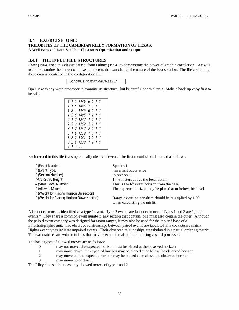
CONOP9 PART B USERS’ GUIDE

38

B.4 EXERCISE ONE: TRILOBITES OF THE CAMBRIAN RILEY FORMATION OF TEXAS: A Well-Behaved Data Set That Illustrates Optimization and Output

B.4.1 THE INPUT FILE STRUCTURES Shaw (1964) used this classic dataset from Palmer (1954) to demonstrate the power of graphic correlation. We will use it to examine the impact of those parameters that can change the nature of the best solution. The file containing these data is identified in the configuration file:

LOADFILE='C:\DATA\rile7x62.dat'

Open it with any word processor to examine its structure, but be careful not to alter it. Make a back-up copy first to be safe.

1 1 1 1446 6 1 1 1 1 1 5 1085 1 1 1 1 1 2 1 1446 6 2 1 1 1 2 5 1085 1 2 1 1 2 1 2 1247 1 1 1 1 2 2 2 1252 2 2 1 1 3 1 2 1252 2 1 1 1 3 1 6 1279 1 1 1 1 3 2 2 1341 3 2 1 1 3 2 6 1279 1 2 1 1 4 1 1 . . .

Each record in this file is a single locally observed event. The first record should be read as follows.

1 (Event Number Species 1 1 (Event Type) has a first occurrence 1 (Section Number) in section 1 1446 (Strat. Height) 1446 meters above the local datum. 6 (Strat. Level Number) This is the 6th event horizon from the base. 1 (Allowed Moves) The expected horizon may be placed at or below this level 1 (Weight for Placing Horizon Up section) 1 (Weight for Placing Horizon Down-section) Range extension penalties should be multiplied by 1.00 when calculating the misfit.

A first occurrence is identified as a type 1 event. Type 2 events are last occurrences. Types 1 and 2 are “paired events.” They share a common event number; any section that contains one must also contain the other. Although the paired event category was designed for taxon ranges, it may also be used for the top and base of a lithostratigraphic unit. The observed relationships between paired events are tabulated in a coexistence matrix. Higher event types indicate unpaired events. Their observed relationships are tabulated in a partial ordering matrix. The two matrices are written to files that may be examined after the run, using a word processor.

The basic types of allowed moves are as follows: 0 may not move; the expected horizon must be placed at the observed horizon 1 may move down; the expected horizon may be placed at or below the observed horizon 2 may move up; the expected horizon may be placed at or above the observed horizon 3 may move up or down;

The Riley data set includes only allowed moves of type 1 and 2.

CONOP9 PART B USERS’ GUIDE

39

The names of the events and sections and critical stratigraphic units may be identified in dictionary files (listed in appendix)

SECTFILE='C:\DATA\riley7.sct' LABELFILE=’C:\DATA\riley.lbl’ EVENTFILE='C:\DATA\riley62.evt'

But these files are optional. If the names are entered as “OFF” the program uses only section and event numbers. If the label file is “OFF,” the program does not label any stratigraphic intervals. Using names for sections and events greatly improves the intelligibility of output. For large data sets, it is not really practical to use numbers instead of names. By contrast, the labels for stratigraphic units are just a neat touch for some graphical output that draws composite sections. Any characters may appear after the string “OFF.” Thus, the dictionaries may be switched off and on without retyping the whole name.

SECTFILE='OFFC:\DATA\riley7.sct' LABELFILE=‘OFFC:\DATA\riley.lbl’ EVENTFILE='OFFC:\DATA\riley62.evt'

Notice that the input file is sorted on three fields. The primary sort is event number (ascending), the secondary sort is event type and the third sort is section number. The CONSORT program will perform this sort for an unsorted preliminary file identified in the .CFG file as follows

PREPFILE='C:\DATA\rile7x62.dis'

CONSORT writes the sorted file to the file name and path listed as the LOADFILE. Notice that the use of stratigraphic height and level number is redundant. The program works in level numbers where possible, because this ordinal tracking is much more efficient; stratigraphic height is used to compute penalties and to prepare output. CONSORT calculates the level numbers from the heights and enters them in the LOADFILE; so, the level numbers on the PREPFILE may be arbitrary integers (but not blanks).

B.4.2 THE GRAPHICAL OUTPUT Repeat the run with the parameters used in the first section. Exit window that shows the end of the animated range chart and the one that draws up the best solution as a rage chart -- this second window is uncluttered by cooling curves and penalty curves. Now the menu bar will offer up to three new options. A “GRAPHICAL OUTPUT” menu has been offered since the first version of CONOP9. A “TEXT OUPUT” option was added with the 3.3 version; it writes selected files to the default disc folder; nothing insightful happens on screen. In version 4, several options for listing the best sequence were moved from the GRAPHICAL OUTPUT menu to a SCREENLIST menu. The list options tend to be unwieldy for large data sets, but are manageable for the Riley example. New options have been added to all three menus in the progression from version 3 to version 6.

Some of the entries in the “GRAPHICAL OUTPUT” menu are explored below; they offer visual insights into the nature of the solution. The illustrations are black-and-white vector images modified from color bitmaps written from the CONOP9 screen displays with the FILE menu; they may include labels not used on the screen.

CONOP9 PART B USERS’ GUIDE

40

B.4.2.1 TAXON RANGE CHARTS Taxon range charts plot the observed and expected (extended) ranges of events one section at a time. Black lines are observed ranges. Pink lines show range extensions and gray lines plot the expected ranges of taxa not observed in the section. Other colors deal with rare situations in which a range is reversed or the expected range is shifted beyond the observed range. Such cases result from unusual settings for the constraints and allowed moves or because the observed data permit no other means of matching the global sequence.

B.4.2.2 COLLECTION QUALITY Logs of collection quality plot the observed and expected number of events and taxa at each collection level. Horizontal bars to the left of the column plot the observed and expected number of events at each level. Bars to the right plot the observed and expected number of ranges that pass through each collection level.

CONOP9 PART B USERS’ GUIDE

41

B.4.2.3 2-D LINES OF CORRELATION Two-dimensional plots of the graphical LOCs between pairs of sections and between sections and composite sections. The X and Y sections may be changed by typing ‘X’ or ‘Y’ followed by ‘<’, ‘-‘, ‘+’, or ‘>’ to march up ad down the sequence of sections or proceed to the ends of the list. FAD and LAD events plot as the corners of boxes. The open ends of the symbol indicate which direction the events were free to be moved (up or down section). Events that cannot be moved to solve the location task are given square symbols (none in this data set!). There is no symbol unless the event has been observed in both sections Symbols change from green to magenta to indicate the position of the event named at the left of the screen. Use ‘+’ and ‘-‘ keys to step through the sequence of events. Use ‘<’ and ‘>’ keys to jump to start or top of sequence. In addition to the real stratigraphic sections, this plot will walk through all ten options for composite sections that attempt to solve the spacing problem.

B.4.2.4 FENCE DIAGRAMS Fence diagrams plot the expected event horizons as wire-lines between section columns. The basic option draws three fences. The three fences differ in the position of the base line for the fences; they are lined up on their tops, midpoints, and bases respectively. The “swept fence” uses each event horizon in turn as the horizontal base line. The sections are plotted in numerical order unless the SECTFILE species otherwise. If there are too many sections for one screen, the fence is plotted in overlapping portions. Dark colored wire-lines are used if the event horizon at both ends lies within the section. If one end is at a section top or bottom, a light color is used. If both end fall at the top or the base of a section, no line is plotted; these events are expected to lie beyond the limits of both sections.

Because the sequencing task has a purely ordinal solution, expected horizons are always located at collection levels. Placement between these levels does not alter the order of events; so there is no biostratigraphic basis for spreading expected horizons between these levels. And there are usually fewer collection levels than events. As a result, the wire-lines in the fence diagrams tend to cluster into radiating bunches. This may be disconcerting, but it is a proper representation of the extent of the biostratigraphic information. Any attempt to smooth the spacing of the wire-lines implies an assumption about the steadiness of sedimentation. Each of the basic fence diagrams redraws using three-

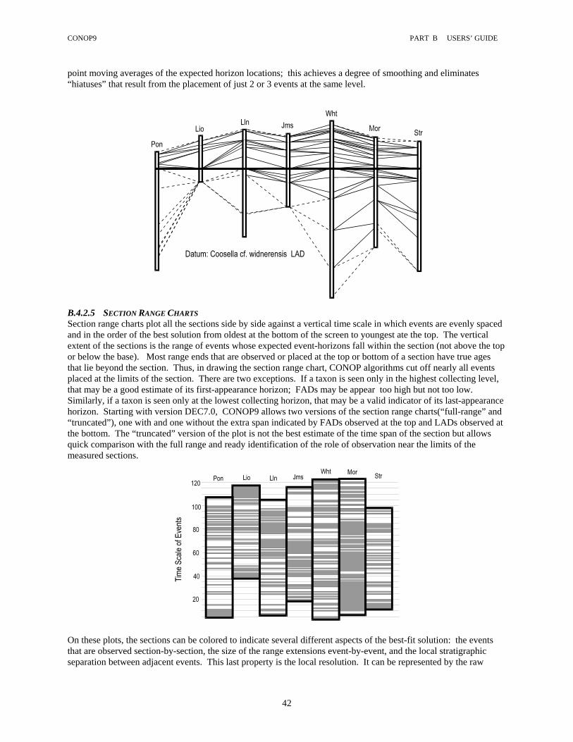
CONOP9 PART B USERS’ GUIDE

42

point moving averages of the expected horizon locations; this achieves a degree of smoothing and eliminates “hiatuses” that result from the placement of just 2 or 3 events at the same level.

B.4.2.5 SECTION RANGE CHARTS Section range charts plot all the sections side by side against a vertical time scale in which events are evenly spaced and in the order of the best solution from oldest at the bottom of the screen to youngest ate the top. The vertical extent of the sections is the range of events whose expected event-horizons fall within the section (not above the top or below the base). Most range ends that are observed or placed at the top or bottom of a section have true ages that lie beyond the section. Thus, in drawing the section range chart, CONOP algorithms cut off nearly all events placed at the limits of the section. There are two exceptions. If a taxon is seen only in the highest collecting level, that may be a good estimate of its first-appearance horizon; FADs may be appear too high but not too low. Similarly, if a taxon is seen only at the lowest collecting horizon, that may be a valid indicator of its last-appearance horizon. Starting with version DEC7.0, CONOP9 allows two versions of the section range charts(“full-range” and “truncated”), one with and one without the extra span indicated by FADs observed at the top and LADs observed at the bottom. The “truncated” version of the plot is not the best estimate of the time span of the section but allows quick comparison with the full range and ready identification of the role of observation near the limits of the measured sections.

On these plots, the sections can be colored to indicate several different aspects of the best-fit solution: the events that are observed section-by-section, the size of the range extensions event-by-event, and the local stratigraphic separation between adjacent events. This last property is the local resolution. It can be represented by the raw

CONOP9 PART B USERS’ GUIDE

43

stratigraphic thickness of intervening rock, or it can be standardized to eliminate differences in thickness and time span from section to section. The standardization process allots an arbitrary 1000 thickness units to the whole sequence. Each section is allotted a fraction of this thickness according to the fraction of all the expected events that fall within the span of the section. Within the section, the allotted thickness is apportioned between events with the according to the relative thickness separations.

Several of the section range charts are drawn with two different color scales, one arithmetic and one logarithmic. The logarithmic scale offers more insight for properties that are characterized by many small values and a few very large ones.

CONOP9 PART B USERS’ GUIDE

44

B.4.3 THE OUTPUT FILES Output files arise in five ways. The RUNLOGFILE is hard-wired to record the run parameters and the initial solution. One set of files is predetermined by the settings in CONOP9.CFG. Others are selected from the “TEXT-FILE OUTPUT” menu after the run has completed. A third group is written as a consequence of selections from the “GRAPHICAL OUTPUT” menu. Typically, the third group is not needed unless there are anomalies in the graphics that need to be diagnosed. In response to prompts that accompany the graphics, blocks of data and text may be appended to the RUNLOGFILE. A fourth type of file includes any bitmap files that save the graphical output screens. These are generated via “SAVE” bar in the Windows “FILE” menu. After completing the search, the program writes three text files (UNLOADMAIN, UNLOADSECT, UNLOADEVNT) that summarize many aspects of the run and the solution. The files contain data and text explanations; they are not suited to reading by machine. The explanations include the names of data files in which blocks of data are written to disk without text explanations. In early versions of CONOP9, the contents of the three files were written as one (UNLOADFILE):

UNLOADFILE='C:\CONOP\output.txt'

Now the names and contents of the three text files are determined by three sets of .CFG settings:

&getout COLUMNS=7 UNLOADMAIN='outmain.txt' FITS_OUT='ON' CNFG_OUT='ON' SEQN_OUT='ON' INCR_OUT='ON' LOC_OUT='ON' OBS_OUT='ON' COMP_OUT='ON' UNLOADSECT='outsect.txt' SECT_OUT='OFF' UNLOADEVNT='outevnt.txt' EVNT_OUT='OFF' COEX_OUT='OFF' . . .

The UNLOADMAIN file has a title that identifies the name and size of the data set and the duration of the run, followed many components that may be independently turned OFF or ON: the best fit, briefly dissected by section and cast in some standardized ratios that permit comparison between data sets; the parameters in the .CFG file that determined the nature and duration of the run; the best sequence of events; the incremental penalties by event and section; the line of correlation (the placed levels of events in every section); the observed levels by event and section; and a representation of the solution as a composite stratigraphic section. The UNLOADSECT and UNLOADEVNT files may be very large and tend to elaborate on material written to the UNLOADMAIN file. UNLOADSECT details the best solution section by section. UNLOADEVNT has two components. The first details the solution event by event; the second spells out all the coexistences that have been reconstructed from the field observations or included by COEX=’FILE’. These files may occupy lots of disk space and take significant time to write after the animated range chart has stopped. If the mode of solution is repetitive (PAUSES=’AUT’ or PAUSES=’RPT’) the time spent writing and re-writing these files may account for most of the run time! Turn most of the options OFF. Remember, after the best solution has been found it is always possible to run the problem again, starting from the best solution, with no search steps or trials, and with all the report options turned ‘ON.’ This gets back to the solution immediately, writes the output analysis and offers the graphical output menu. The following lines from the configuration file determine the destination of the uncommented data files. These files reproduce the data tables from the UNLOADMAIN text file, without explanatory text so that they may easily be

CONOP9 PART B USERS’ GUIDE

45

parsed and read by machine. They are written automatically and may be examined with a word processor or loaded into a spreadsheet. Each run overwrites these files unless the names are changed. Notice that the full suite of data files together with a complete output text file will amount to a considerably larger volume of information than the input data. This is one consequence of automated analysis. The familiar warning about “garbage-in garbage-out” stresses the need for high quality input data. There should be a second warning that concerns quantity: “inches-in, miles-out”.

. . . RUNLOGFILE='runlog.txt' CULLFILE='cull.txt' SOLNLIST='solution.sln' STARTFILE='soln.dat' STEPFILE='stepsoln.txt' BESTARTFILE='bestsoln.txt' COMPOSFILE='cmpst.dat' . . . OBSDFILE='ab.dat' PLCDFILE='albet.dat' EXTNFILE='delta.dat' COEXISTFILE='coex.dat' ORDERFILE='ordr.dat' /

RUNLOGFILE records a few run-time parameters like the initial sequence, the anomalies in the pairwise event spacing option of the graphical output menu.

CULLFILE is under development. It will record the results of the culling circle option of the graphical output menu.

SOLNLIST can store solutions from several runs so that they may be compared. STARTFILE stores the end point of the search and may be used to continue the search from this

sequence. It is the best-fit answer to the sequencing task. STEPFILE stores the solution at the end of each step in the cooling schedule. It allows recovery of

progress if the run crashes or must be cut off before the end. BESTARTFILE stores the best known solution for a set of runs based on the lowest values in

CURVFILE. It prevents the best solution from being lost if a new run is started from a random sequence.

COMPOSFILE stores a composite section in a format suitable for use as part of an input file. OBSDFILE stores the observed levels of events by section; it repeats the input data PLCDFILE stores the placed/expected levels of the event horizons by section. It is the response to the

locating task and may be considered to be the coordinates of the multi-dimensional line of correlation.

EXTNFILE stores the misfits/range extensions by event and section. It is the difference between the observed and placed horizons.

COEXISTFILE records the coexistence matrix; one row and one column for every paired event. ORDERFILE records the partial ordering matrix; one row for every unpaired event; one column for every

event. B.4.4 CHANGING THE CONSTRAINTS In the standard run, coexistences were proved by the loose rules of evidence. Change the .CFG file to the strict rules of evidence and re-run the program to determine whether the solution is sensitive to the difference.

FORCECOEX='SL' | ‘SS’ | ‘OFF’

It is possible to drop the constraints that observed ranges cannot contract, but this often has unrealistic consequences. The ease with which individual observed ranges may be extended can be altered by changing the weighting factors at the end of each record in the input file. Notice that weights can be tailored to individual sections and taxa. An event that currently incurs a large misfit in a given section (significant range extension) may be stabilized by increasing its weighting factors. The sensitivity of the solution to that local observation is revealed by the size of the extent to which changing its weight can change the whole best-fit solution. The well-behaved nature of the Riley data means that there are so many local events with consistent relationships from section to

CONOP9 PART B USERS’ GUIDE

46

section that the solution is reasonably resilient to changes in one local observation. (This is not true for the Mohawk data set, used in a later exercise.) B.4.5 CHANGING THE MEASURE OF MISFIT The standard run gave reported the misfit in terms of five different measures. But the search optimized the INTERVAL penalty. Change the penalty parameter in the .CFG file to find the best solution for the other measures of misfit.

PENALTY=’INTERVAL’ | ’LEVEL’ | ’ORDINAL’ | ’SPATIAL’ | ’SEQUEL’ || ’ROYAL’ | ’RASCAL’

The different measures can produce quite different ranges of misfit values. To achieve an efficient search, other parameters must be adjusted to account for this. The easiest single adjustment alters the value of STARTEMP, which will be explained in section 5. The best-known solutions and reasonable settings for STARTTEMP are as given in the table below. In essence, the STARTEMP parameter should be smaller when the measure of misfit assumes smaller values. For a well-behaved dataset, however, there is considerable leeway.

PENALTY BEST FIT

STARTEMP

STARTYPE

RATIO

HOODSIZE

STEPS

TRIALS

FORCECOEX

INTERVAL 3546 100-200 RAND 0.98 ‘BIG’ 500 100 SL LEVEL 204 10-20 RAND 0.98 ‘BIG’ 500 100 SL ORDINAL 533 10-100 RAND 0.98 ‘BIG’ 500 100 SL SPATIAL 1102 20-100 RAND 0.98 ‘BIG’ 500 100 SL RASCAL 186.9 10-20 RAND 0.99 ‘BIG’ 500 100 SL ROYAL 40 20-50 RAND 0.98 ‘SMALL’ 500 2000 SL SEQUEL 435 50-100 RAND 0.98 ‘SMALL’ 500 2000 SL

If many runs are undertaken with different measures, it will be noticed that a series of solutions may have the same misfit value for one measure but a range of different values for another measure. The reason is that for any one measure of misfit, there are pairs of larger combinations of events that may change places in the sequence without changing the misfit. Typically, the same events are not interchangeable for all measures of misfit. For runs that optimize the ‘ROYAL’ penalty (with Fb4L constraint), the ‘INTERVAL’ penalties may range from 3900 to 4100, but the ‘SEQUEL’ penalties may all be near optimal, because the SEQUEL and ROYAL penalties are so closely related for small, well behaved correlation problems. STARTEMP, RATIO, HOODSIZE, STEPS, and TRIALS are parameters that determine the progress of the search for the best solution. Although they are not explained properly until later sections, they do matter for experiments with the full range of measures of misfit (PENALTY). The search proceeds by trial and error; it guesses at a sequence of events and then applies a series of mutations, looking for improved fit to the observed sections. HOODSIZE determines the nature of the mutation between each trial. The other parameters determine whether errors (bad mutations) are removed or left in the sequence of changes. Because the size of the misfit values changes across two orders of magnitude with the different penalty functions, the size of the mutation is also critical to the ability of the search to converge consistently onto the best solution. The ‘ROYAL’ penalty is so small, that the big mutations (or big neighborhood structure - HOODSIZE=’BIG’) do not converge on the best penalty in every run; try it; final values will probably vary between 40 and 46. The ‘SEQUEL’ penalty has the same problem in combination with the BIG mutations (look for likely variations from 435 to 450). For these two measures of misfit, convergence is considerably improved by using the small mutations (HOODSIZE=’SMALL’). DOUBLE mutations swiftly alter the sequence of events; they do not converge well on the optimal solution for any measure of misfit. Notice that the small mutations require more trials and the smaller penalty values can use lower STARTEMP values. B.4.6 COMPARISON WITH SHAW'S SOLUTION Solutions found by constrained optimization and traditional graphic correlation are very similar. The results can be compared qualitatively on range charts or with graphic correlations of the two solutions. Differences are small and

CONOP9 PART B USERS’ GUIDE

47

non-systematic, except that constrained optimization produces slightly better economy of fit. Kendall's (1975, p. 94) coefficient of concordance, W, quantifies the similarity of the solutions derived by annealing from different initial sections. Perfect concordance results in a value of 1.00. For pairs of solutions derived from different local sections, W is always greater than 0.98; comparison of these solutions with the one derived from Shaw's solution produces W's of 0.95. For correlation purposes, the differences are probably not worth the effort of making multiple searches from different starting points. KENDALL'S RANK CORRELATION OF INTERVAL SOLUTIONS

Simulated Annealing Solutions (Runs differentiated by source of Initial Permutations)

Traditional Graphic Correlation (Shaw’s Solution)

Section 4 Section 6 Shaw’s Solution Section 1 .9831

.9754*

.9814**

.9864

.9733*

.9900**

.9899

.9770*

.9938**

.9509

.9361*

.9505** Section 4 .9826

.9708*

.9527**

.9881

.9843*

.9843**

.9525

.9374*

.9566** Section 6 .9899

.9768*

.9973**

.9484

.9321*

.9507** * range-beginning events only ** range-ending events only Shaw's solution required many pages of ad hoc justification for LOCs. Mostly he was selecting the better established local ranges, and the exercise had an air of subjectivity. Our comparable solution is particularly noteworthy because we used no subjective weights for the taxa or the sections. We conclude that the complete set of local observations serves to identify the better established ranges. A reasonable solution in J dimensions can arise without elaborate weighting schemes. But constrained optimization is fast enough that it is possible to experiment with truly subjective opinions about the quality of different taxa and sections. Differences in the final solution that result from different subjective weights will indicate where subjective opinion really matters and which parts of the data set have little influence on the outcome. Similar insights might be gained from studying the contributions of different taxa and sections to the penalty for the best solution. Such sensitivity analyses indicate where additional sampling would be most profitable. Although the discrete scale of event horizons is entirely sufficient for the sequencing task, the solution obtained by constrained optimization appears crude by comparison with Shaw's (1964) results when both are plotted as a fence diagram. Constrained optimization bunches the lines of correlation because it places expected event horizons (a

ij

's and b

ij

's) only at horizons where fossils have been collected or sought. The more even spacing of events in Shaw's (1964) solution results solely from the assumption that the ratios of accumulation rates between sections do not change. B.4.7 LIMITATIONS OF THE TRADITIONAL GRAPHIC METHOD Shaw’s (1964) method encounters serious limitations because it integrates the records of local stratigraphic sections one at a time. The method proceeds by series of partial correlations, the first between two local sections, the rest between one local section and the developing composite section (Shaw, 1964; Miller, 1977; Edwards, 1989). Many of these essentially two-dimensional steps are required to integrate all the data and each step appears deceptively simple. Unfortunately, in the early steps, the two-dimensional graphs contain only a small fraction of the total information. As a result, the early LOCs are difficult to draw and likely to be of low quality. And yet the results of the early steps have the strongest impact on the final outcome (Edwards, 1984). The placement of lines of correlation (LOCs) depends heavily on subjective judgments, especially in the early steps. First, the partial correlations begin with the two sections judged to have the greatest abundance of reliable observations. Secondly, the LOCs are rarely fit equally to all observations. Shaw (1964, p. 235-241) explained in

CONOP9 PART B USERS’ GUIDE

48

detail how to select a subset of presumably more reliable local observations. His selection process relies on a knowledge of observations in stratigraphic sections not yet included on the graph. Another popular tactic tries to route the LOC between the first and last occurrence observations so that range adjustments impact the section judged to be least reliable and minimize changes in the composite section (MacLeod and Sadler, 1995). This tactic extends the influence of judgments about the relative reliability of sections. Subjective judgments that are used to constrain the early LOCs continue to influence the outcome after all sections have been integrated. In an attempt to remove the biases introduced by the early partial correlations, Shaw (1964) repeated the whole procedure several times. At the start of each reiteration, the composite section produced by the previous iteration serves as the initial section. But the composite is first modified to remove the impact of one section -- a irksome step, unless computer-assisted. Reiteration is a tedious exercise with progressively diminishing returns. But without it, the final composite cannot fairly reflect all local observations. CONOP solves the correlation problem for all J sections at once. It eliminates any need to consider the sequence of inclusion of the local sections; it is like a J-dimensional graphic method in which every section occupies an axis from the start. The J-dimensional LOC records the best sequence without recourse to a composite section. There is no need to dedicate an axis to a composite section and there is no question of routing the LOC to separate first and last occurrences. Because all the local observed event horizons are available as objective data from the outset, none of this information is used selectively. Thus, much apparent subjectivity in the traditional method simply disappears. In order to make partial correlations with the limited information on a two-dimensional graph, the traditional approach preferred a straight LOC (Shaw, 1964) or one with very few "doglegs" (Miller, 1977). In some instances, however, the implication that sections maintain a constant ratio of accumulation rates is too severe a simplification. Graphic correlation of cores from the Deep Sea Drilling Project with one another and against time scales (e.g., Pisias and others, 1985) has shown that straight lines of correlation can be unrealistic, even for abyssal marine accumulation. For marine sections on the shelf and continental slope, seismic stratigraphy has shown that the stratigraphic record is dominated by prograding wedges of sediment in which the site of maximum accumulation rate probably oscillates onshore and offshore with the rise and fall of sea level (Vail and others 1977). This leads to the prediction that changes in the accumulation rates of inner shelf, outer shelf, and slope sections should be out of phase with one another and not lead to straight LOCs. Thus, sedimentologic and stratigraphic support for the assumption of a constant ratio of accumulation rates may be quite weak, compared with the paleontological evidence for the sequence of events. It is sound practice to solve the stratigraphic correlation problem without initial constraints based upon accumulation rate. Modern implementations of graphic correlation routinely permit piecewise-linear LOCs (MacLeod and Sadler, 1995) and, thus, prevent sedimentologic assumptions from dominating the paleontological evidence for the sequence of events. B.4.8 ADVANTAGES OF THE TRADITIONAL GRAPHIC METHOD Traditional graphic correlation has a very significant advantage, especially for those new to numerical correlation methods. The 2-D graphs on which each step is completed make everything very explicit. They offer considerable insight and prevent many errors. In other words, although the case for eliminating subjectivity is very compelling, and although subjective solutions may be biased and poorly reproducible, subjective solutions are almost always reasonable and understood by their developers, even novices. Finally, subjectivity is expertise, and not all of a stratigrapher’s expertise can be fed into programs like CONOP and RASC. It is informative (and not always flattering) to the stratigrapher to ask: why not? For the full Mohawk problem (the exercise given in this manual, plus the conodonts and lithological units) manual graphic correlation produces much more satisfying answers. The Mohawk data are not yet sufficient to support a unique objective solution. B.4.9 THE INITIAL SOLUTION Shaw (1964) started his graphic compositing with section 1 (Morgan Creek). One table in this section summarizes experiments with several different initial sequences, all using the INTERVAL penalty. A few were random, one was Shaw's solution, and most were based upon the sequence of observed event horizons in a local section. Unlike an initial section in traditional graphic correlation, CONOP’s initial sequences must include all events and respect

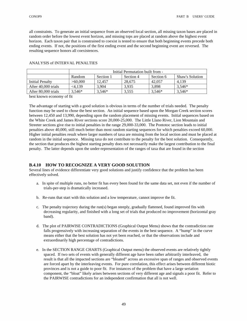
CONOP9 PART B USERS’ GUIDE

49

all constraints. To generate an initial sequence from an observed local section, all missing taxon bases are placed in random order before the lowest event horizon, and missing tops are placed at random above the highest event horizon. Each taxon pair that is constrained to coexist is tested to ensure that both beginning events precede both ending events. If not, the positions of the first ending event and the second beginning event are reversed. The resulting sequence honors all coexistences. ANALYSIS of INTERVAL PENALTIES Initial Permutation built from - Random Section 1 Section 4 Section 6 Shaw's Solution Initial Penalty >60,000 12,457 28,675 42,057 4,139 After 40,000 trials <4,139 3,904 3,935 3,898 3,546* After 80,000 trials 3,546* 3,546* 3,555 3,546* 3,546* best known economy of fit

The advantage of starting with a good solution is obvious in terms of the number of trials needed. The penalty function may be used to chose the best section. An initial sequence based upon the Morgan Creek section scores between 12,450 and 13,990, depending upon the random placement of missing events. Initial sequences based on the White Creek and James River sections score 20,000-25,000. The Little Llano River, Lion Mountain and Streeter sections give rise to initial penalties in the range 29,000-33,000. The Pontotoc section leads to initial penalties above 40,000, still much better than most random starting sequences for which penalties exceed 60,000. Higher initial penalties result where larger numbers of taxa are missing from the local section and must be placed at random in the initial sequence. Missing taxa do not contribute to the penalty for the best solution. Consequently, the section that produces the highest starting penalty does not necessarily make the largest contribution to the final penalty. The latter depends upon the under-representation of the ranges of taxa that are found in the section B.4.10 HOW TO RECOGNIZE A VERY GOOD SOLUTION Several lines of evidence differentiate very good solutions and justify confidence that the problem has been effectively solved.

a. In spite of multiple runs, no better fit has every been found for the same data set, not even if the number of

trials-per-step is dramatically increased. b. Re-runs that start with this solution and a low temperature, cannot improve the fit. c. The penalty trajectory during the run(s) began steeply, gradually flattened, found improved fits with

decreasing regularity, and finished with a long set of trials that produced no improvement (horizontal gray band).

d. The plot of PAIRWISE CONTRADICTIONS (Graphical Output Menu) shows that the contradiction rate

falls progressively with increasing separation of the events in the best sequence. A “hump” in the curve means either that the best solution has not yet been reached, or that the observations include and extraordinarily high percentage of contradictions.

e. In the SECTION RANGE CHARTS (Graphical Output menu) the observed events are relatively tightly

spaced. If two sets of events with generally different age have been rather arbitrarily interleaved, the result is that all the impacted sections are “bloated” across an excessive span of ranges and observed events are forced apart by the interleaving events. For pure correlation, this effect arises between different biotic provinces and is not a guide to poor fit. For instances of the problem that have a large seriation component, the “bloat” likely arises between sections of very different age and signals a poor fit. Refer to the PAIRWISE contradictions for an independent confirmation that all is not well.

CONOP9 PART B USERS’ GUIDE

50

B.4.11 A WARNING ABOUT LARGER DATA SETS The Riley data set is small enough that the searches may be repeated many times in order to become confident that the best solution has been found. Very large data sets may require runs of several days (or weeks). These are much less convenient to repeat, but no less likely to be “stuck” in a sub-optimal solution. As the data sets get larger it becomes increasingly important to run conservatively long searches with slow cooling schedules in order to avoid seriously sub-optimal solutions. Remember, the solution does not necessarily become uniformly better throughout the search. Some parts of the best sequence may be found relatively early but local bad features may survive much longer. Exercise two illustrates the problems with a small dataset. The reference entries under PAUSES=”AUT” suggest a conservative cooling schedule that adjusts to the rate at which mutations are leading to improvements of fit. This setting is recommended for all large data sets. It may be applied to the Riley data set to see how it works. Set PAUSES=’AUT’, STEPS=50 and TRIALS = 10000; start the programs; watch and wait!. Each temperature will be held for 10000 mutations. If any improvement is found, another 10000 trials will be initiated at the same temperature (results are first written to disc and the screen repaints, be patient). If no improvement occurs, the temperature is lowered. If the temperature is lowered 50 times in succession without improvement, the program stops. Notice that TRIALS and STEPS are now “stopping rules” that allow the program to decide when to cool and when to stop. B.4.12 VARIANTS OF THE RILEY PROBLEM Some CDs include modified versions of the Riley data set that illustrate the use of different event types based upon fossil taxa. To explore them, alter the input lines in CONOP9.CFG B.4.11.1 UNPAIRED TAXON EVENTS The following set of input files breaks each taxon range down into two unpaired events, an appearance (APP) and a disappearance (DIS).

RILE7x124.DAT with RILEY124.EVT and RILEY7.SCT

In addition to these filenames, CONOP9.CFG must include the following altered settings, because ‘TAXA’ refers only to the number of FAD-LAD pairs and FAD-MID-LAD triplets. All unpaired events go into the ‘EVENT’ count.

. . . SECTIONS=7 TAXA=0 EVENTS=124 . . .

In this data set there is an APP and a DIS for all 62 taxa so that the results can be compared with the standard Riley results. APP and DIS events need not be matched. This data set will not give results comparable with the paired data, unless the paired data are run without coexistence constraints. Although unpaired events can prove coexistences, there is no enforcement of constraints for unpaired events. The animated range chart will show a twinkling of yellow dashes -- there are no paired ranges. Notice that the appearances are all listed before the disappearances and therefore plot in the top half of the screen. This is convenient but not mandatory. B.4.11.2 MID-RANGE TAXON EVENTS The following set of input files includes four appearance (APP) and disappearance (DIS) events together with a demonstration of five mid-range events.

RILE7x62x9.DAT with RILEY66.EVT and RILEY7.SCT

In addition to these filenames, CONOP9.CFG must the following settings, because ‘TAXA’ refers only to the number of FAD-LAD pairs and FAD-MID-LAD triplets. All unpaired events go into the ‘EVENT’ count. But the mid-range events do not add new event numbers or taxon numbers; therefore the EVENTFILE has only a 66 count (62 taxa plus the 2 APP and 2 DIS events) not the 71 that you might expect from the following.

CONOP9 PART B USERS’ GUIDE

51

. . . SECTIONS=7 TAXA=62 EVENTS=9 . . .

The animated range chart will show 62 white ranges plus four yellow dashes for the APP and DIS events. The five mid-range events plot as red segments in the corresponding white range bars. They should never jump out of the white ranges. The 5 mid-range events are arbitrary and fictitious. They could be used to represent ‘acme’ events and test their viability for correlation. The inclusion of an option for mid-range events should not be taken as an endorsement for acme zones. To the contrary, they were first included as a means to expose the flaws in the concept.

CONOP9 PART B USERS’ GUIDE

52

_____________________________________ B.5 SIMULATED ANNEALING

In order to be able to find the best solution for larger datasets, or those with a higher percentage of contradictions, it is necessary to pay more attention to the settings for the search heuristics -- parameters in the configuration file that do not change the nature of the best solution but do determine the efficiency of the search. Stratigraphic correlation belongs to a class of problems termed "strongly Non-Polynomial Complete" (Dell and others, 1992). This means that the computation time increases exponentially (or faster!) with the number of sections and taxa in the problem. Other optimization problems that can be NP-complete include searching for the shortest cladogram, locating airline hubs, and routing traveling salesmen. Fortunately, research into these problems has led to a number of general-purpose algorithms that, properly adapted, often find the best solutions for small instances and very good solutions for large ones, without calculating the penalty for every feasible solution. They start with one possible solution and attempt to apply a series of modifications that progress toward better solutions without trying every possibility. The most successful search technique for the biostratigraphic correlation problem is called simulated annealing (Kirkpatrick et al., 1983; Kemple et al., 1995). B.5.1 STARTING POINTS FOR THE SEARCH All searches require a feasible sequence to use as a starting point. A feasible sequence includes all events and must honor the constraint settings such as coexistences. Conop offers three options for the starting sequences: a random sequence (STARTYPE=’RAND’); a sequence based upon one of the local sections with missing events added randomly (STARTYPE=’SECT’); and a sequence read from a specified file (STARTYPE=’FILE’ | ‘STEP’ | ‘BEST’). The third option is used to string several searches together in series in order to be sure of finding the very best fit. Two or three files are written during the run: the file named in STARTFILE records the best solution found in the last run; BESTARTFILE records the best-known solution across a series of runs that use the same data; and STEPFILE may be used to establish a file that records the solution at the end of one step in the annealing process. Every search supplies its best solution to the file designated for starting sequences (STARTFILE) and may update the best-known solution (BESTARTFILE). The viability of the BESTARTFILE depends upon activating a suitable record of previous best solutions. The file that records the best fits as a function of the position of each event (CURVEFILE) serves this purpose; it must not be turned OFF. The behavior of the STEPFILE is determined by its setting in the configuration file (CONOP9.CFG). It is possible to write these files manually, but the user must ensure that the sequence is complete and satisfies all constraints and coexistences. Conop checks these qualities and makes corrections automatically for the sequences it generates. If the initial solution is called from a file with the wrong number of events, the program will terminate with a corresponding error message. If the number of events is correct but the constraints are not honored, the run might be “trapped in a very bad neighborhood that is difficult to exit.” The following sections explain the significance of this jargon.

STARTFILE=’C:\CONOP\soln.dat’ STARTSECT=1 STARTYPE='RAND' | ‘SECT’ | ‘FILE’| ’STEP’ | ’BEST’|’CONT’

B.5.2 A TOPOGRAPHIC ANALOG FOR SEARCH ALGORITHMS Consider how you might walk to the lowest point on an unmapped topographic surface if you could see only your immediate neighborhood. Imagine that the visible neighborhood extends only one small step from your current position in any direction. We could let the landscape represent a two-dimensional linear regression. Because a straight line is specified by its slope and intercept, the misfit corresponding to all possible lines can be contoured on a two-dimensional map. Latitude and longitude on the map are slope and intercept. Step size is fixed by the smallest permitted changes in slope and intercept. Every point on the map represents a different straight line. The elevation of the landscape at any point is the misfit between the corresponding line and the observed data. A

CONOP9 PART B USERS’ GUIDE

53

downhill step improves the fit; uphill steps increase the misfit. The lowest point on the landscape is the best solution.

For two-dimensional linear regression the landscape is a basin with only one minimum; instructions for walking to the lowest point are very simple. Take any step that leads downhill from the current standpoint and repeat until all possible steps lead uphill.

The landscape for the stratigraphic correlation problem is more complex in formulation and in topography. Each point on the landscape now represents a feasible sequence of all events. Elevation is the total misfit that results when that sequence is forced upon all the local sections. Do not worry that it is hard to build a mental image of this landscape. The main point is that landscape is likely to include many closed depressions of different sizes and depths. The search procedure must be able to explore and escape from these local minima, most of which are not optimal (deepest). Therefore, the simulated annealing heuristic provides a means to “climb out of holes.” First we must consider the nature of single steps in the search. Steps from one point to a neighboring point represent small changes in the sequence of events. The neighborhood of a point is all the other points that can be reached form it in one step or one change in the sequence. The rules for making these changes or steps across the landscape determine the so-called neighborhood structure. B.5.3 THE MINERALOGICAL ANALOGY FOR SIMULATED ANNEALING For crystals growing from a cooling melt, Boltzmann distribution law explains why slower cooling increases the probability of growing perfect crystals. Perfect crystals are the minimum energy state. Although the system prefers low energy states at any temperature, higher energy states do arise but with a small probability that decreases as temperature falls. Slow cooling maximizes the likelihood that the final state will achieve the minimum energy. For a fixed temperature (T) greater than zero, Boltzmann distribution gives the probability PT(π) that a state π will arise:

PT(π) = KTe-{E(π)/kbT} (5)

where E(π) is the energy of state π, KT is a normalizing constant which brings the area under the probability distribution to 1, and kb is Boltzmann's constant. Kirkpatrick and others (1983) recognized that the energy of a state is exactly analogous to the penalty for a solution to an NP-complete problem. They proposed a search that allowed "bad" moves with the same probability that a cooling physical system assumed non-minimal energy states. They reasoned that such a search would reliably find the best solution if the probabilities were reduced according to the right schedule, just as efficient annealing schedules can be found that yield perfect crystals. Using a computer to simulate sampling from the distribution given above is difficult because KT is unknown. In fact, enumeration of all possible states for a given T>0 would be required to evaluate KT. Metropolis and others (1953) developed a method of simulation that samples the distribution without evaluating KT. Their algorithm starts at one state, generates a new "neighboring" one, calculates the change in energy (δE) that will occur if the new state (π) is adopted, and accepts the new state according to the probability distribution:

⎧1 , δE<0 PT(π) = ⎨ (6) ⎩e-{δE/kbT}, δE>0

The analogy with the outer optimization and the neighborhood structure of our searches is obvious. Hammersley and Handscomb (1964, p. 117-121) give a fairly readable proof that this algorithm simulates sampling from Boltzmann’s distribution. Simulated annealing exploits the Metropolis algorithm to allow the outer minimization a comparable probability of accepting a change to a new sequence (π): ⎧1 , δF<0 PT(π) = ⎨ (7) ⎩e-{δF/T}, δF>0 where δF is the change in penalty (elevation) associated with the move to p from the current sequence, and T decreases during the search. The constant kb is not needed because we are no longer using real temperature and

CONOP9 PART B USERS’ GUIDE

54

energy scales. The equation says that, although the search prefers to move "downhill" to a sequence with a lower penalty, uphill moves do occur and such moves have a small probability, which decreases with T as the search progresses. The appearance of T in the denominator of the exponent -(δF/T) is the key to the behavior of the search. The range of values assumed by δF depends on the data set and the distance scale used. If the search begins at a value of T that is very large compared with typical values of δF, PT(π) approximates a uniform distribution on the set of all feasible sequences; all moves are approximately equally likely to be chosen regardless of δF. If the search continues until T becomes very close to zero, the probability of accepting any move that increases the penalty now tends to zero regardless of δF. At intermediate values of T, the search is more sensitive to δF; moves that increase the penalty are more likely to be accepted if the penalty increment is small. To simulate the annealing process, the search starts with a high value of T (analogous to a molten state) and lowers it slowly while testing feasible sequences. If T is reduced slowly enough, the search path converges to a sequence with the global minimum penalty (analogous to a perfect crystal). The components of the best cooling schedule are all problem specific and may need to be altered for different sets of data. To get a starting temperature T, first specify an approximate initial value for accepting an uphill move (0.5 worked for us). Next generate a series of neighbors for one sequence and determine the distribution of δF. Finally solve backward for the initial value of T that gives the desired probability. We tried logarithmic cooling as suggested by Geman and Geman (1984). After 100,000 trials, searches on our stratigraphic data sets had not stabilized, so we returned to the stepwise cooling schedule of Kirkpatrick and others (1983). We chose cooling ratios between 0.90 and 0.98 by trial and error and adjusted the number of trials at each temperature to prevent PT(π) from falling too fast. The next section describes the performance of different cooling schedules on one stratigraphic data set. B.5.4 DIFFERENT STEP SIZES After determining the misfit for the current sequence, the search procedure might generate the next one by selecting one event at random and moving to a new random position in the sequence. The configuration file calls the result a “BIG” neighborhood. It is the most efficient structure that we have found for a wide range of data sets. It causes the animated range chart to make the characteristic loom-like motions: one event makes a big change in sequence and all the events between its initial and final positions adjust by one position in sequence.

HOODSIZE='BIG'

Another strategy reverses the order of one pair of adjacent events. It produces a “SMALL” neighborhood and an animated range chart that “twinkles”. The tiny sequence changes allow the misfit to be recalculated very rapidly by a process of re-optimization. Unfortunately, a thorough search needs so many tiny changes that the search becomes increasing inefficient as the size of the data set grows. The “SMALL” neighborhood becomes relatively smaller (net change is only one rank) as the length of the sequence grows. By contrast, the size of the “BIG” neighborhood grows with the length of the sequence because the possible changes range from one rank to the total number of ranks in the sequence. Because almost every local section misses a few of the events in the global sequence, even the BIG neighborhood structure can take advantage of some aspects of reoptimization. For this reason, the BIG structure is automatically run with “partial reoptimization.” For SMALL step sizes, full reoptimization was employed if specified, in version prior to 6.0.

HOODSIZE=‘SMALL’ [ + ‘REOPT’ prior to version 6.0]

After version 6.0 the general unsuitability of the SMALL neighborhood was so apparent that the specially tailored REOPT option was eliminated. While the SMALL neighborhood algorithm is relatively easy to update with other changes to the program (e.g. event types), the reoptimization algorithms were complex and troublesome to update. A more radical strategy for changing the sequence swaps two events at random. This “DOUBLE” neighborhood allows the search to move rapidly away from random starting positions; but it is usually too coarse to find the very best solution at the end of the search. For very large data sets may be efficient to perform a short search with the double neighborhood structure and use the outcome as the starting sequence for a big-neighborhood search.

HOODSIZE=‘DOUBLE’

CONOP9 PART B USERS’ GUIDE

55

B.5.5 STRINGING THE STEPS TOGETHER Simulated annealing picks possible steps at random in the current neighborhood. Each step is evaluated to determine whether it should be accepted as the starting point for the next step or whether it should be reversed and a different step attempted from the previous position. Steps that happen to lead downhill are always accepted. If an uphill move is selected, a carefully adjusted probability structure (based on equation 7) determines whether to accept the move or try another random selection in the same neighborhood. The probability of accepting a large uphill move is always set smaller than the probability of accepting a small uphill move. The probability of accepting an uphill move of a given size is made to decrease progressively throughout the search. In effect, the searcher progressively tires. Early in the search, it is possible to climb large-scale barriers in the landscape because the searcher has strength for large uphill steps and long runs of successive uphill steps. Thus, simulated annealing begins by sounding the large-scale topography and tends to home in on the slopes around the global minimum. Toward the end of the search, an exhausted searcher makes mostly downhill steps and can descend precisely to the lowest point. B.5.6 COOLING SCHEDULES For human searchers on a landscape, we would need to specify the initial vigor and a tiring schedule. The initial vigor determines the chances of moving uphill away from the starting point; a high value is more desirable if the starting point is separated from the lowest point by significant relief on the landscape (e.g., a random starting sequence that is far from the optimal sequence). In practice, a stepped schedule for tiring the searcher is easier to manage than a smooth curve. After a fixed number of TRIALS at each STEP, vigor is reduced by a constant tiring RATIO. The fixed tiring ratio (less than one) ensures that the likelihood of uphill moves decreases less rapidly toward the end of the search and never reaches zero. The slowest tiring schedules give the searcher a high initial vigor, a high tiring ratio (close to 1.0), enough cooling steps that vigor is very close to zero at the end of the run, and a large number of trials between each reduction in vigor. Because slow tiring schedules allow significant uphill movement late into the search, they work best from bad starting points on very rough landscapes. They waste too many moves if the starting point is good or the landscape simple.

STEPS=500 TRIALS=100 STARTEMP=200 RATIO=0.98

To specify the formula that converts vigor into a probability distribution for accepting uphill moves, Kirkpatrick et al. (1983) derived their formula by analogy with Boltzmann's distribution law from statistical mechanics. Accordingly, it is usual practice to speak in terms of initial "temperature" and a "cooling" schedule, rather than the initial vigor and tiring schedule of our qualitative analog.

To simulate the process of annealing and then slow cooling to grow a perfect crystal, the search starts with a high temperature (analogous to a molten state) and lowers it slowly while testing feasible sequences. If temperature is reduced slowly enough, the search path converges to a sequence with the global minimum penalty (analogous to a perfect crystal). The components of the best cooling schedule are all problem specific and may need to be altered for different sets of data. CONOP9 uses the most popular form of cooling schedule. It uses small temperature reductions and a fixed number of trials at each temperature. Some authors compare such schedules with ‘inhomogeneous’ Markov Chains. The alternative model (homogeneous Markov Chains) holds the temperature constant until enough trials have been attempted to ensure that the system comes close to some equivalent of thermodynamic equilibrium. The equilibrium concept is difficult. But the strategy is straightforward -- monitor the improving fit to determine when it is appropriate to lower the temperature. Although the number of trials at each temperature may be rather large, proponents claim that larger temperature changes may then be used. The alternate strategy implies that there is a problem with fixing the number of trials at every step: perhaps this number is too large at some temperatures and too small at others. It is possible to instruct CONOP9 (version 6.0 or

CONOP9 PART B USERS’ GUIDE

56

later) to set up a cooling schedule that remains at each temperature as long as improvements can still be found. This is achieved by setting the PAUSES parameter to ‘AUT’ (for AUTomatic). Refer to the reference entry for this parameter to learn how the STEPS and TRIALS parameters are used to tailor this option. Very briefly, TRIALS now determines the minimum number of trials at each temperature and STEPS provides the stopping rule -- the maximum number of consecutive lowerings of temperature that will be attempted without any improvement in the solution before the program concludes that the search is finished. Properly tailored, the resulting search becomes very thorough, but may be rather slow. The option is perhaps best suited to searches of huge data sets that should be left to churn for several days rather than investing the same time looking for the most efficient cooling schedule. This “intelligent” cooling schedule was developed for such huge data sets and not included in CONOP until version DEC6.0 of CONOP9. It has been tested far less that the fixed cooling schedules that have been used successfully since the earliest versions of CONOP2 to solve a wide variety of biostratigraphic problems. B.5.6.1 Sample Cooling Schedules -- The following schedules have been successful for the problem sizes given, but there is no assurance that problems of the same size have the same proportions of observed events or comparable levels of contradiction.

7 SECTIONS WITH 62 TAXA: solver = ‘anneal’ penalty = ‘interval’ showmovies = ‘cht’ pauses = ‘on’ steps = 500 trials = 100 starttemp = 200 ratio = 0.98

[less than 1/2 minute to solution; PENTIUM II; 400mHz; 128mb RAM; NT4 ] [less than 1/2 minute to solution; PENTIUM III; 600mHz; 32mb RAM; WIN98 ] [less than 1/3 minute to solution; PENTIUM IV; 1600mHz; 1Gb RAM; WIN98 ]

27 SECTIONS WITH 131 TAXA: solver = ‘anneal’ penalty = ‘level’ showmovies = ‘cht’ pauses = ‘on’ steps = 500 trials = 500 starttemp = 100 ratio = 0.98 20 SECTIONS WITH 177 TAXA AND 19 OTHER EVENTS: solver = ‘anneal’ penalty = ‘interval’ showmovies = ‘cht’ pauses = ‘on’ steps = 500 trials = 1000 starttemp = 100 ratio = 0.98 195 SECTIONS WITH 638 TAXA AND 38 OTHER EVENTS: solver = ‘anneal’ penalty = ‘level’ showmovies = ‘div’ pauses = ‘aut’ steps = 50 trials = 10000 starttemp = 100 ratio = 0.98

[2-3 days to best solution; PENTIUM III; 400mHz; 128mb RAM; NT4] [3-4 days to best solution; CELERON; 500mHz; 128mb RAM; WIN98]

198 SECTIONS WITH 1170 TAXA AND 38 OTHER EVENTS: solver = ‘anneal’ penalty = ‘level’ (short preliminary run with ‘ordinal’)

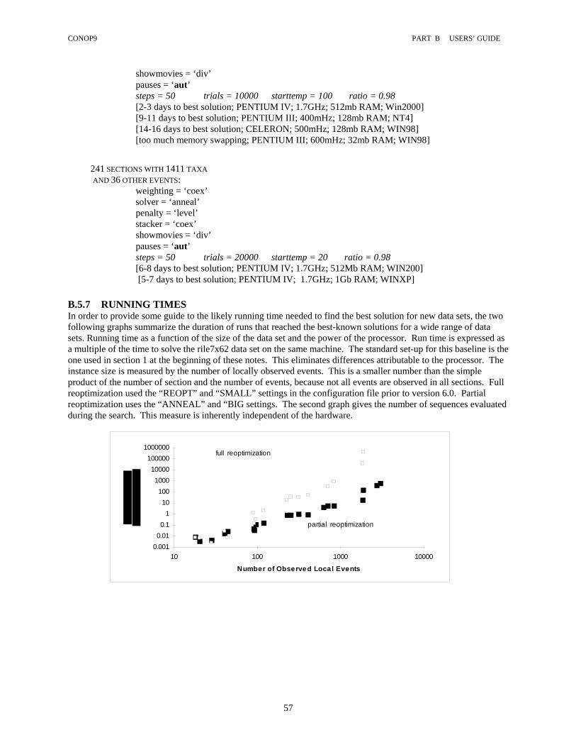
CONOP9 PART B USERS’ GUIDE

57

showmovies = ‘div’ pauses = ‘aut’ steps = 50 trials = 10000 starttemp = 100 ratio = 0.98

[2-3 days to best solution; PENTIUM IV; 1.7GHz; 512mb RAM; Win2000] [9-11 days to best solution; PENTIUM III; 400mHz; 128mb RAM; NT4] [14-16 days to best solution; CELERON; 500mHz; 128mb RAM; WIN98] [too much memory swapping; PENTIUM III; 600mHz; 32mb RAM; WIN98]

241 SECTIONS WITH 1411 TAXA AND 36 OTHER EVENTS: weighting = ‘coex’ solver = ‘anneal’ penalty = ‘level’ stacker = ‘coex’ showmovies = ‘div’ pauses = ‘aut’ steps = 50 trials = 20000 starttemp = 20 ratio = 0.98

[6-8 days to best solution; PENTIUM IV; 1.7GHz; 512Mb RAM; WIN200] [5-7 days to best solution; PENTIUM IV; 1.7GHz; 1Gb RAM; WINXP]

B.5.7 RUNNING TIMES In order to provide some guide to the likely running time needed to find the best solution for new data sets, the two following graphs summarize the duration of runs that reached the best-known solutions for a wide range of data sets. Running time as a function of the size of the data set and the power of the processor. Run time is expressed as a multiple of the time to solve the rile7x62 data set on the same machine. The standard set-up for this baseline is the one used in section 1 at the beginning of these notes. This eliminates differences attributable to the processor. The instance size is measured by the number of locally observed events. This is a smaller number than the simple product of the number of section and the number of events, because not all events are observed in all sections. Full reoptimization used the “REOPT” and “SMALL” settings in the configuration file prior to version 6.0. Partial reoptimization uses the “ANNEAL” and “BIG settings. The second graph gives the number of sequences evaluated during the search. This measure is inherently independent of the hardware.

Number of Observed Local Events

0.0010.010.1

110

1001000

10000100000

1000000

10 100 1000 10000

partial reoptimization

full reoptimization

CONOP9 PART B USERS’ GUIDE

58

110

1001000

10000100000

100000010000000

1000000001000000000

10000000000

10 100 1000 10000

Number of Observed Local Events

Num

ber o

f Tria

ls to

Sol

utio

n

part ial reopt imizat ion

full reopt imizat ion

The following generalizations summarize the factors that influence the running time:

i. Running time increases with the number of STEPS and TRIALS; the product of these two values determines the number of solutions to be evaluated.

ii. Running time increases with the number of SECTIONS and EVENTS; the product of these two values determines the number of horizons to be placed.

iii. Running time increases with the number of event-section combinations that are actually observed; this value determines the number of horizons for which a penalty must be calculated; it can be found using CONTROL9 or in the reports from CONOP9.

iv. Running time increases with the number of trials that are accepted, including uphill moves. Thus, the running time tends to increase as the initial temperature increases or the cooling ratio increases; i.e. it increases with temperature at any stage of the search.

v. Ordinal penalties (ORDINAL, RASCAL, SPATIAL) and the coexistence penalty (ROYAL) can be calculated much faster than interval penalties (INTERVAL, LEVEL) because there is no need to place horizons to evaluate ordinal penalties.

vi. RASCAL is slower than ORDINAL; it must normalize the count of contradictions. vii. SPATIAL is slower than ORDINAL because it must measure the separation of observed events. viii. If the solution is written to disk at the end of each step (STEPFILE not ‘OFF . . .’ ), the duration of

each step is appreciably increased, especially for large data sets. For data sets that exceed 1000 taxa, the writing time may be measured in minutes (depending upon hardware). Why take the time? For large data sets that run for hours or days, this is insurance against interruption. It also allows the run to be stopped deliberately and restarted for any reason, e.g. transporting a lap-top computer between locations..

ix. The automatic cooling schedule (PAUSES=’AUT’) is built to reach the best solution unattended but without regard for speed. Two factors slow the AUT setting. First, each temperature is held until the stopping rule indicates that sufficient unsuccessful trials have been attempted. Second, there are many housekeeping chores to complete at the end of each run of trials. Also, it is often advisable that the solution and the temperature be written to disc at the and of each run of trials (STEPFILE). This enables the run to be interrupted without loss of the findings. For a large data set, these writing actions and other housekeeping chores at the end of each run of trials may take longer than the trials themselves.

x. Addition of a secondary penalty (SMOOTH, SHRINK, SQUEEZE, TEASE) slows the search considerably.

xi. Of the STACKER options, OLAP is the fastest because it does not need to loop through all the sections. COEX avoids sections too, but must query the coexistence matrix. INCL may be about 5 times slower than OLAP.

CONOP9 PART B USERS’ GUIDE

59

B.5.8 OTHER COOLING PROTOCOLS Some algorithms in the Simulated Annealing literature set up significantly different cooling protocols. The following have been noted. They are not operational in CONOP9; rather, reasons are offered to believe that the simple geometric cooling in CONOP approximates the same desirable features.

1. Permit heating or cooling -- increase the temperature after every accepted move, reduce it after every rejected move. The heating and cooling ratios are specified separately. It is possible to determine the size of the temperature change by the size of the misfit change. This could be regarded as a more complicated way of slowing the cooling than the simple plateaus (TRIALS) in the geometric cooling schedule.

2. Variable repetition factor -- increase the number of trials at each temperature (length of the temperature step) throughout the run, as the temperature is lowered. At each step the new number of trials is generated from the previous number via a constant multiplication factor that should be fixed at a value between 1.0 and 2.0. It is asserted that lower temperatures require more trials to ‘equilibrate.’ Ratio cooling ensures that the temperature steps are smaller at low temperature; thus the desired effect may be achieved without the variable repetition factor.

3. Cooling rules -- allow the program to remain at one temperature until improvement is no longer likely. The PAUSES=‘AUT’ setting allows a fixed number of trials (TRIALS) to be repeated at the same temperature until none of them finds a better sequence.

4. Stopping rules -- allow the program to continue until it ‘recognizes’ that improvement has ceased; the recognition criterion is a stopping rule. The goal is to ensure that the run is long enough to find the best solution. The obvious inconvenience is not-knowing when the run will be finished; for a very large data set this is a small price to pay. The basic CONOP9 schedule fixes the length of the cooling schedule in advance. One parameter setting in CONOP9 (PAUSES=’AUT’) introduces a stopping rule. The animated range chart offers another possibility: open a STEPFILE to ensure that the solution is written to disk at the end of every cooling step; set STEPS and TRIALS to make a longer run than necessary; watch the animation to determine when the improvement has ceased; interrupt the program; restart a 1-step run from STEPFILE (FILE=’STEP’) in order to write out the full analysis of the STEPFILE solution.

The founders of Simulated Annealing recommended a logarithmic cooling schedule. A large body of early literature agrees that the stepped geometric cooling schedule (fixed cooling ratio) is more effective. B.5.9 PARALLEL SIMULATED ANNEALING Parallel simulated annealing has not been programmed for CONOP9. It would involve running parallel searches as different threads, perhaps taking advantage of multiple processors. B.5.10 TWO-STAGE ANNEALING The recent literature in operations research has made much of two-stage simulated annealing (TSSA). This heuristic starts with a faster or more aggressive search, then switches to traditional simulated annealing -- before getting trapped in a local minimum. The trick is to stop the first stage soon enough and start the second stage with the right temperature. Although TSSA is not offered as a single solver option, a pair of runs may be used to mimic this heuristic. The first run exploits search strategies that are fast but unlikely to converge on the desired answer. The solution from the first run is fed to a second run in which the search parameters are adjusted to converge on the best solution. There are four basic ploys that can be built into this approach in different combinations. Notice that none of them can be set intelligently for a new data set. Their judicious use must be learned for each data set.

i. Use a more aggressive search strategy for the first stage. Either use a low STARTEMP or set the SOLVER to the GREEDY algorithm option, which accepts only improvements (see below). Both of these approaches tend to fall into local minima.

ii. Use a penalty setting in the first stage that is faster to calculate than the desired penalty. ORDINAL and ROYAL penalties can be calculated without making local range extensions. The ORDINAL penalty will almost always produce a reasonable start. If the desired penalty includes a secondary term based upon coexistences (STACKER=’COEX’), then ROYAL may be well suited to the first stage. Bear in mind that the ROYAL penalty needs to derive its sense of polarity from the sequence of taxa in local sections or from

CONOP9 PART B USERS’ GUIDE

60

dated events, or from a series of marker beds observed in superposition. Sets of taxa that lack these indications of polarity may be placed in rather arbitrary positions in the solution.

iii. Stop the first stage before the solution incorporates bad elements from which it cannot escape. Start the second stage cooling schedule so that iterative improvement continues where the first stage terminated.

iv. Let the first stage run most of the way to its best solution. Then start the second stage at a high enough temperature to allow the prior solution to relax its fit. The relaxation (anneal and quench) should be sufficient to climb out of any local minima.

B.5.11 ADAPTIVE SIMULATED ANNEALING An adaptive simulated annealing (ASA) algorithm analyzes the trajectory of the penalty function in order to decide when the temperature should be lowered. In other words, the program ASA programs have an internal stopping-rule and a stepping-rule so that the cooling schedule adapts to the instance of the problem at hand. Some ASA allow the temperature to step up or down; some adjust both the size and direction of temperature change. The idea is to ensure that each temperature step in the cooling schedule is maintained as long as it is still efficient or, in the landscape analogy, as long as necessary to make a thorough search at that scale. Much of the ASA literature speaks in terms of reaching equilibrium at each step and many implementations look at the ratio of accepted and rejected moves to identify “equilibrium”. The trade-off is speed -- the extra time needed to analyze the trajectory. Some of the lost speed may be recovered by making larger cooling steps. No sophisticated ASA option has been included with CONOP9. The setting PAUSES=’AUT’ tries to adapt the number of TRIALS at each temperature to wait until improvements are no longer found. The Reference section explains how to control the cooling schedule with this option. B.5.12 SIMULATED TEMPERING True simulated tempering is a variant of simulated annealing in which the temperature may move up or down; temperature changes are selected at random, but the decision whether or not to accept the change is driven by a probability function including the Boltzmann constant and the time since the search began. In other words, misfit and temperature have traded roles in the heuristic. The implementation in CONOP is less elegant; it uses numerous short, fast cooling runs or “quenches;” the starting temperature for each quench is selected at random and always accepted; the Metropolis selection criteria are applied to misfit during each quench. Tempering permits vigorous hill climbing anywhere in the search and becomes a viable alternative for solving very badly behaved data sets.

SOLVER=‘TEMPER’

As implemented by conop9, the number of tempering quenches is given by “STEPS.” The duration of each quench is given by TRIALS and the temperature is reduced by the RATIO after every trial. Therefore, relative to annealing, steps needs a smaller value while trials and ratio must be set to higher values. The following combination is suited to small data sets with less than ten sections and 30-130 events.

SOLVER='TEMPER' PENALTY='INTERVAL' STEPS=20 TRIALS=5000 STARTEMP=50 RATIO=0.999

The practical uses of the simulated tempering option are limited. The option was designed as a means of exploring the full set of equally-well-fit and nearly-best-fit. It has some potential for solving highly conflicted data sets for which the misfit landscape is very rough at several scales. B.5.13 THE GREEDY ALGORITHM Greedy searches are easy to program, but rarely successful. They may look at the whole neighborhood or single neighbors, but always accept the steepest downhill move and readily get trapped in local minima. The chance of finding the true minimum can be increased by restarting the greedy search several times using different starting

CONOP9 PART B USERS’ GUIDE

61

sequences - “greedy algorithm with random restarts.” For some very simple instances of the correlation problem, multiple greedy searches perform faster than more complex single search algorithms. But the suitability is difficult to know in advance for any given instance. Because the greedy algorithm accepts only downhill steps, it has little value for finding the best-fit solutions. But it can be used to map out local minima or establish best-fit intervals. Temperature and cooling settings are not relevant for greedy runs, except that the product of the values entered for STEPS and TRIALS determine the length of the run.

SOLVER=‘GREEDY’

When a secondary penalty is applied at the end of the primary run in simulated annealing (e.g. SOLVER = ’TEASE’), the primary penalty follows greedy rule (it never increases) while the secondary penalty seeks to choose among solutions that are equally well-fit to the observed data. B.5.14 TABU SEARCH If a greedy algorithm could remember the path into local minima, it might learn to climb out and seek deeper minima. Tabu search (Glover, 1990) attempts to give the greedy algorithm this kind of intelligent memory. The search keeps "tabu lists" of past moves and updates them as it moves about the landscape. It still evaluates the entire neighborhood at each step but selects its best move after eliminating steps that are on the current tabu list. The lists have fixed length and a first-in-first-out maintenance rule (each update adds a new tabu move to the top of the list and drops one from the bottom). Longer lists retain moves longer. A tabu search program must specify the general character of sequence changes that can become tabu. Obvious tabu rules attempt to prevent repeated visits to the same location. An event that has recently been moved higher to generate a new sequence might be prohibited from moving back down as long as it is listed. A pair of events that have switched places might not be allowed to switch back until dropped from the list. At run time, the tabu lists keep track of specific events to which the rules will apply each time the outer minimization generates a new sequence. Multiple lists with different lengths are permitted. Long lists resemble long-term memory because past events remain longer on the list. Obviously tabu search is not a rigidly specified procedure. It gives memory and whole-neighborhood searching their place in a flexible template for tailoring an intelligent search. In addition to fixing parameters like the number and length of tabu lists, it is necessary to discover rules that identify potentially bad sequence changes. Dell et al (1992) have tried to apply Tabu Search to the correlation problem. They were unable to find “rules” that could make a tabu search more efficient than simulated annealing. So, CONOP9 does not include a tabu searching option. The large number of optional parameters in Tabu Search bring great flexibility and a source of weakness -- the learning curve is longer and steeper than for simulated annealing; Tabu Search is relatively inscrutable. For biostratigraphic correlation problems, the time required to learn and “tune” a tabu search, is better spent on annealing runs. B.5.15 GENETIC ALGORITHMS I have not found any reasonable way to adapt the strengths of genetic algorithms to the stratigraphic correlation and seriation problems. The difficulty lies in the narrowly-constrained nature of feasible sequences -- all events may appear only once and every FAD must precede the corresponding LAD. As a result, I have not found any efficient means to generate viable hybrids from the mating of two suboptimal sequences. Simple cutting and splicing fails spectacularly. It remains far more efficient to work with one sequence. A mechanism comparable with “mutations” in the sequence is already fundamental to the generation of new sequences in simulating annealing. Of course, it is possible to run a family of parallel searches, periodically eliminate the apparently less successful ones, and use the best individual as the starting point for a new family of searches. The individual searches might vary as a result of random effects or be set up with different cooling schedules. The snag is that “success” would need to be judged from the interim best penalties. Unfortunately, the interim penalties are not always a good guide

CONOP9 PART B USERS’ GUIDE

62

to proximity to the global minimum; a greedy search, stuck in a local minimum, could easily look best in the short term. Nov. 01: At the 2001 Annual Meeting of the Geological Society of America, Roy Plotnick presented a means of solving correlation problems with a genetic algorithm. It proceeded directly to the Line of Correlation (LOC). The number of linear segments on the LOC was chosen in advance. The genetic algorithm mutated the position of the segment ends until the best fit was found. The number of segments was progressively increased until diminishing returns were found. In effect, by keeping the number of segments much smaller than the number of events, the method gains considerable efficiency relative to CONOP. Two general questions follow. First, how efficiently would simulated annealing solve the problem if it were recast in the same LOC-based fashion? In other words, is the increased efficiency due to the genetic algorithm or the LOC-based statement of the problem? Second, can the LOC-based approach be used efficiently to solve seriation problems? In other words, what special difficulties arise when some pairs of sections have no overlap in time. Jan. 02: Michael Foote (pers. comm. 2002) has suggested a possibility for GA-like hybridizations within CONOP. Rather than trying to merge coherent halves of two sequences, the sequence in one might guide the mutations of the other. It would work like this: pick an event at random in the sequence to be mutated; try moving it to its position in the other sequence; if this is not possible, move it as far as possible toward its position in the other sequence; if this is not possible, pick another event at random; repeat until half of the events have been moved?

CONOP9 PART B USERS’ GUIDE

63

B.6 EXERCISE TWO: GRAPTOLITES OF THE MID-ORDOVICIAN OF THE MOHAWK VALLEY: A Poorly-Behaved Data Set That Illustrates Annealing Options Goldman et al. (1994) built a new chronostratigraphic model for the upper Middle Ordovician of the Mohawk Valley using 21 graptolite taxa, 24 conodont taxa, and ash beds from eight measured sections. Their model departs significantly from an older one based on less biostratigraphic information and a different interpretation of the ash stratigraphy (Cisne and Rabe, 1978; Cisne et al., 1982a,b).

The two models differ markedly in their treatment of the limestone turbidites of the Dolgeville facies. Using the old model, this facies appears to be a persistent platform apron. The section at Dolgeville Dam (section D of Goldman and others, 1994) was interpreted to overlap considerably in age with the section at Flat Creek (section B). According to the new model, the limestones are a relatively brief pulse and most of the section at Dolgeville Dam is younger than the section at Flat Creek.

The data in mo6x21x7.dat include the 21 graptolite taxa (see appendix for listings) and the six sections from which Goldman et al. (1994) recovered graptolites. Sadler and Kemple (1995) analyzed the same problem but omitted six of the graptolites because they were found in only one section. The data set here includes 5 tuff beds for which the correlation is uncontested and two radiometric dates. The dates are fictitious, but lie in uncontroversial parts of the record; they illustrate how to include such events; but do not influence the outcome. The conodont taxa provide little guidance in correlation. Their ranges are long compared with the time span of local sections and they are recovered from the limestones. As a result, the conodonts force spurious correlations between the limestone intervals. B.6.1 TWO REGIONS WITH VERY GOOD FIT With a moderately rapid cooling schedule, the Mohawk data yield a solution with an interval misfit in the range 579-610. These solutions broadly resemble the correlations proposed by Cisne et al. (1982). With a more conservative cooling schedule or a long series of simulated temperings, a better fit can be found. It resembles the correlation proposed by Goldman et al. (1994).

CONOP9 PART B USERS’ GUIDE

64

B.6.2 THE SOURCE OF THE AMBIGUITY The two solutions differ markedly in their treatment of the correlation between the Flat Creek section and the Dolgeville Dam section. The 610 solution retains much of the observed sequence from Flat Creek and correlates the Dolgeville Dam with the heart of the Flat Creek section. The 461 solution resembles the Dolgeville Dam sequence and places most of this section above the Flat Creek section. The correlation between the Dolgeville and Nowadaga sections vary little between the two solutions. The Caroga Creek, Chuctanunda Creek and Wolf Hollow sections have the same relationship to Flat Creek in both solutions.

CONOP9 PART B USERS’ GUIDE

65

Wolf Hollow

Nowadaga

Dolgeville

CarogaFlat

Chuctanunda

45

40

35

30

25

20

15

10

5SOLUTION 610

The outcome rests on the treatment of the contradictions between observed sequences at Dolgeville Dam and Flat Creek. A graphic plot of the shared taxa between these two sections reveals irreconcilable differences contradictions. Taxa 7 and 9 require massive adjustments in both sections to bring them to a common chronostratigraphic model. Taxa 1, 3, and 10 must be adjusted significantly in one or other of the two sections. Evidently, these two sections should be targeted for more collecting, if possible, to resolve contradictions.

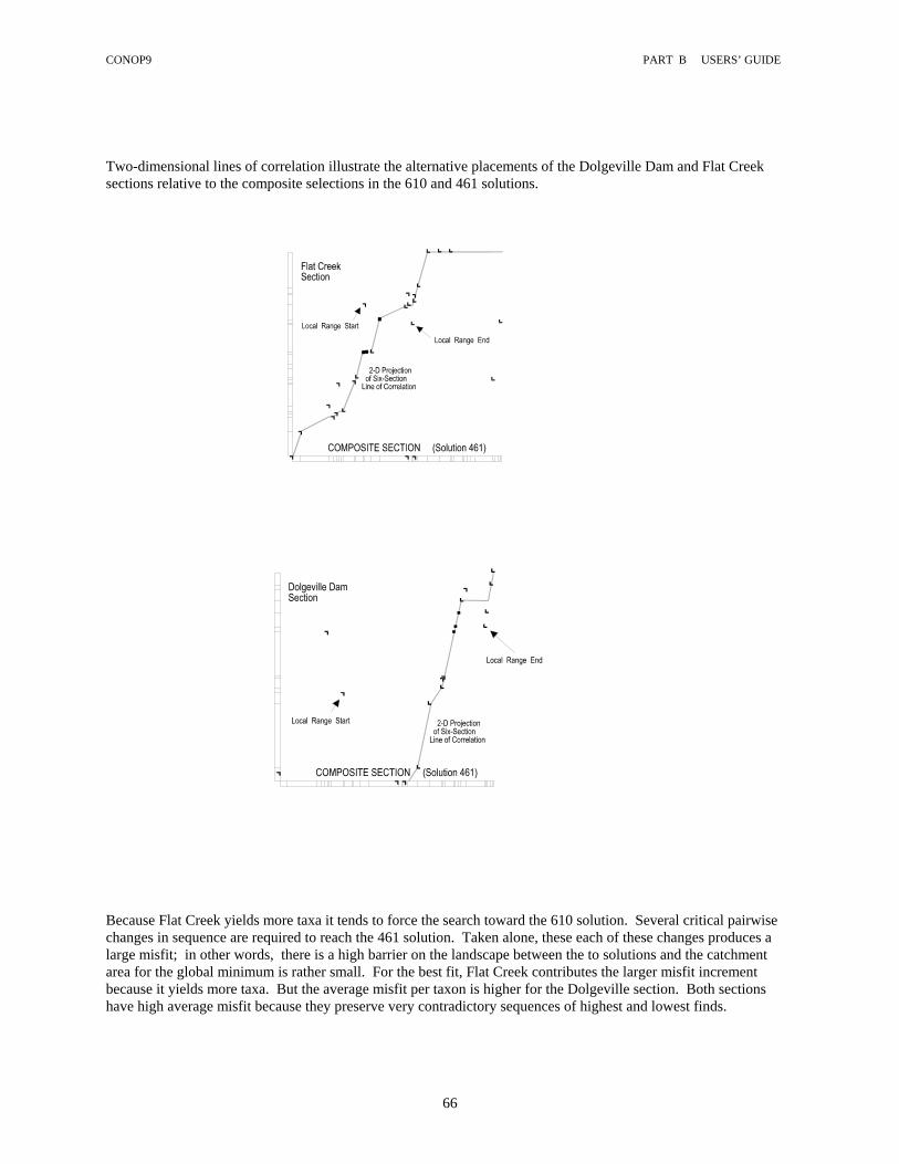
CONOP9 PART B USERS’ GUIDE

66

Two-dimensional lines of correlation illustrate the alternative placements of the Dolgeville Dam and Flat Creek sections relative to the composite selections in the 610 and 461 solutions.

Because Flat Creek yields more taxa it tends to force the search toward the 610 solution. Several critical pairwise changes in sequence are required to reach the 461 solution. Taken alone, these each of these changes produces a large misfit; in other words, there is a high barrier on the landscape between the to solutions and the catchment area for the global minimum is rather small. For the best fit, Flat Creek contributes the larger misfit increment because it yields more taxa. But the average misfit per taxon is higher for the Dolgeville section. Both sections have high average misfit because they preserve very contradictory sequences of highest and lowest finds.

CONOP9 PART B USERS’ GUIDE

67

The resolution of the problem must be sought in new stratigraphic data from one of these sections. Either an extension of a currently known range or a new tuff correlation could easily shift the balance between the alternative chronostratigraphic models.

B.6.3 TUNING THE SEARCH TO THE BEST FIT Finding a cooling or tempering schedule that will consistently and efficiently discover the best known solution for the Mohawk data is a serious challenge. It will be faced for any instance of the problem that generates a landscape with local minima that are widely separated. On the misfit landscape of a well-behaved instance like the Riley Formation, there are few closed depression and they are all close to the best-fit solution; in other words, the minima all lie in the same catchment area and it is possible to move from one to the other late in the search with few uphill moves. The Mohawk problem has minima that are separated into distinct catchments with a relatively high altitude barrier between them. And, to make the search more difficult, the global minimum seems to lie in a relatively small catchment. The diagram below shows the distribution of local minima as discovered by numerous greedy searches with random starting positions. The bar that represents the 461 solution is quite short relative to the 610-579

CONOP9 PART B USERS’ GUIDE

68

solutions; this relationship indicates that a relatively small portion of the landscape lies on slopes that lead downhill to the best fit or 461 solution

The distribution of local minima is much more favorable on the misfit landscape for the Riley Formation. The local minima are relatively closely spaced, and the largest catchment area leads down to the global minimum. The figure for the Riley Formation also indicates the advantage that the search can achieve by starting from a local section rather than a random sequence of events.

Obviously, much insight can be gained from maps of the frequency distribution of values (altitudes) on the misfit landscape. Also, frequency distributions of paths that lead to local minima (closed depressions) are excellent guides to the selection of search strategies. Unfortunately, the computation time to map these distributions corresponds to thousands, or tens of thousands, of normal runs.

Because efficient searches of the Mohawk misfit-landscape must climb substantial barriers late in the search, simulated tempering has more promise than for instances of the correlation problem with fewer internal contradictions. A simulated tempering with 30 or more quenches performs better than most other searches.

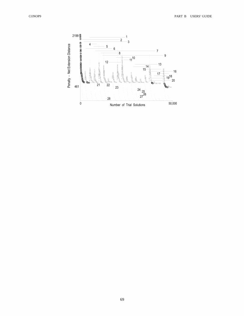
CONOP9 PART B USERS’ GUIDE

69

CONOP9 PART B USERS’ GUIDE

70

B.7 RELATIONSHIP OF CONOP TO CLADISTICS This section is excerpted from an NSF proposal by Sadler, Hughes, and Webster, that was funded for three years commencing July 2000. B.7.1 MISSING QUESTIONS Two questions have dominated the interaction between cladistics and biostratigraphy: whether cladistic estimates of phylogeny expose real gaps in the fossil record; and how best to incorporate stratigraphic information in the search for the most parsimonious cladogram (Wagner, 1998). Although many have argued that cladistic evidence of phylogeny is superior to stratigraphic evidence, a third question has received surprisingly little attention: whether cladistic estimates of the order of origination of taxa might improve the resolution of biostratigraphic correlation. Unfortunately, the existing strategies for integrating stratigraphy and cladistics cannot be readily adapted to this purpose. They must fail in high-resolution studies because they ignore the internal contradictions in the stratigraphic record. Thus, a fourth question arises: whether cladistic analysis can incorporate stratigraphic data in a fashion that deals with these contradictions and remains robust at high-resolution. To resolve contradictions within the stratigraphic record, CONOP has given correlation a mathematical formulation (Kemple et al., 1989, 1995) which is comparable to that used in cladistic analyses to resolve morphological ambiguities. This opens new possibilities for integrating the two tasks. Because correlation considers the appearance and disappearance of taxa, section by section, and cladistic analysis considers morphologic characters, taxon by taxon, the taxa appear to be the link between the two tasks. But cladistics does not reconstruct the succession of species; it reconstructs the succession of morphologic events (Remane, 1985). Consequently, the answer to the missing questions does not become “yes” until correlation is recast to consider the appearance of morphological character states rather than taxa. To provide a secure foundation for the following discussion, we must first be explicit about the taxonomic and stratigraphic properties of a “high-resolution” analysis: The taxonomic working level is not higher than species; No species in the clade recovered from the target time interval is excluded from consideration (i.e. the cladogram is not limited to exemplar species); So many species are included that the average spacing of origination events is shorter than the resolution of absolute age calibration; The stratigraphic time span is long enough, relative to the average species duration, that some of the preserved fossils are likely to be ancestors of others in the study (Foote, 1996); The relative age of origination events is established by their position in vertically contiguous sets of strata in stratigraphic sections, not by recourse to absolute age calibration; and Numerous sedimentary sections are used, each including many species, and each potentially recording time intervals missing in some of the other sections (Sadler and Strauss, 1990). These are the characteristics of all studies that lead to robust biostratigraphic zonation. Moreover, these are the scales that methods of phylogenetic analysis should aim to reach, because fundamental evolutionary processes operate at these scales. Cladistic analysis and correlation should share information at all scales, and especially at high-resolution where sharing is most vital. B.7.2 SEPARATE BUT EQUALLY DIFFICULT OPTIMIZATION TASKS Fence diagrams and trees summarize the solutions of correlation and cladistic analysis respectively. Both icons embody a sequence of origination. Stratigraphic correlation seeks lines that connect horizons of the same age in separate sedimentary sections. The sections are posts in the fence diagram. The lines in the fence maintain the same order from post to post. Most of the lines usually purport to trace the time of origination or extinction of fossil taxa, but they could equally well trace the appearance of individual morphological traits. Available data always constrain the sequence of tie lines better than the spacing between them. The true age of the lines is typically the most speculative aspect of the fence.

CONOP9 PART B USERS’ GUIDE

71

Cladistic analysis seeks to arrange taxa at the tips of a tree. Depending upon the cladist’s point of view, the tree either inherently expresses evolutionary relationships or forms a basis for discovering them. Trees combine three types of information: topology, taxon labels at the tips of the tree, and branch length (node spacing). Each pectinate branch on a rooted tree fixes the order of its nodes; each node represents a change in state of one or more characters. Trees and fences are built from quite different information, but their methods of construction converge in order to deal with incongruency in large data sets. Fence construction begins with range charts that record the span of preservation of fossil taxa at each section. The charts underestimate the true taxon ranges because preservation and collection are imperfect. The degree of underestimation varies from place to place, and so the sections contradict one another in detail concerning the relative duration of species and the sequence of origination events. Trees are based upon similarities in morphological and/or biochemical properties of taxa. Tree construction must deal with the ambiguity inherent in similarity: rather than evidence of true kinship, similarity may be a misleading homoplasy, the result of parallel or convergent evolution. To resolve the contradictions and ambiguities, both tasks are usefully framed as constrained optimizations that are well-suited to automated heuristic methods (“stepwise addition” and “branch-swapping” for trees, “simulated annealing” and “tempering” for fences). By comparing potential solutions to the empirical observations, these methods iteratively improve the solution. They use intelligent trial-and-error to minimize objective functions that measure the total implied incongruency in the data. Both optimizations typically

Part of the parsimony tree for olenelloid trilobites (after Lieberman, 1998, fig. 2).

Fence diagram drawn by CONOP to show the correlation of 7 sections from the Cambrian Riley Formation of Texas, using 62 taxa, mostly trilobites (data from Palmer, 1954, in Shaw, 1964) Horizontal datum line: Maryvillia cf. arista FAD.

CONOP9 PART B USERS’ GUIDE

72

generate sets of rival solutions -- equally most-parsimonious trees or equally best-fit fences -- that share the lowest known value for the objective function. The most parsimonious trees minimize a function based on the number of implied homoplasies. The best-fit fences minimize the contradictions with the local stratigraphic observations and the implied failures of preservation and collection in the fossil record. Changing the objective function, the constraints, or the weights, used in either optimization usually yields a different set of rival solutions. A unique best solution rarely emerges for either task. But we place greater confidence in those portions of the tree or fence that are common to all rival solutions and those that emerge unchanged by the use of different measures, constraints, and weights. The typical solution is a set of rival best-fit sequences. The whole set can be represented as a string of overlapping circles in which the larger circles identify less well constrained events -- those that can occupy a wider range of positions in the set of equally best-fit sequences. Alternatively, CONOP9 can construct confidence curves for each event; the curves illustrate how the best-known fit changes as the event is moved through all possible positions in the sequence and the other events are reoptimized. Contributions to the total misfit can be subdivided to evaluate individual sections, events, or sets of events. B.7.3 STRATIGRAPHIC INFORMATION IN CLADISTIC ANALYSES Computer programs such as PAUP (Swofford, 1991, 1998), PHYLIP (Felsenstein, 1989) and MACCLADE (Maddison and Madison, 1994) automate the task of constructing phylogenetic trees. Such automated, quantitative methods of optimization enjoy much wider application by cladists than among biostratigraphers. Not surprisingly, therefore, the best-known attempts to integrate stratigraphy and cladistics are applications of stratigraphic information to cladistic analysis (summaries in Hitchin and Benton, 1997; Siddall, 1998; Wagner, 1998). The goals have been to add extinct ancestral taxa that help root the parsimony trees, to choose between equally parsimonious trees (Fischer, 1992; Huelsenbeck, 1994), and to support the more recent views that a near-most-parsimonious tree might be the best estimator of phylogeny (Wagner, 1998). Three quite different operational strategies emerge for integrating stratigraphic information. One strategy compares the sequence of appearances in the fossil record with the sequence of originations implied by the most-parsimonious trees. Although whole sequences may readily be compared using Spearman’s rank correlation coefficient (Gauthier et al., 1988), trees that are not fully pectinate do not resolve the relative ages of all originations. It is then necessary to prune away the unresolved parts (Norell and Novacek, 1992) or treat each node separately (Huelsenbeck, 1994). A different strategy, also based on end-product, assesses the gaps and ghost taxa that a parsimony tree implies for the stratigraphic record (Norell, 1992; Smith and Littlewood, 1994; Benton and Storrs, 1994; Benton and Hitchin, 1996; Foote, 1996; Foote et al., 1999). Other measures being equal, this second strategy prefers the tree that implies the minimum stratigraphic ‘debt’ (Fischer, 1991, 1994). The third strategy includes stratigraphic information among the input properties of the taxa that are subject to cladistic analysis. Stratigraphic information may be optimized alongside the traditional characters (Fischer, 1991, 1994; Siddall, 1998), or traditional data may be re-weighted after comparing initial results with the stratigraphic record (Huelsenbeck, 1994). Discussion of the relative merits of these strategies has tended to focus on topological aspects of trees. Let us take a biostratigraphic point of view. Although the last two strategies avoid some problems inherent in rank correlation, they use the most tenuously estimated stratigraphic information. Evidence for the absolute age of origin of a taxon, or the elapsed time between two origination events, is almost inevitably more tenuous than the evidence of relative age of events or their position in a sequence of events. Confidence intervals should accompany estimates of origination times to avoid worrying about implied gaps that are not statistically significant (Wagner, 1995; Marshall, 1998). In addition to uncertainties inherited from the age calibration, confidence intervals on taxon range ends lengthen with the rarity of a taxon and the duration of its observed range. Unless the observed range of a fossil is established on six or more separate finds, reasonable estimates of the confidence interval may be substantially longer than the observed range (Strauss and Sadler, 1989). For the sequence of appearances to be confidently compiled on a global time scale, the origination times must be more widely separated than both the confidence intervals on the range

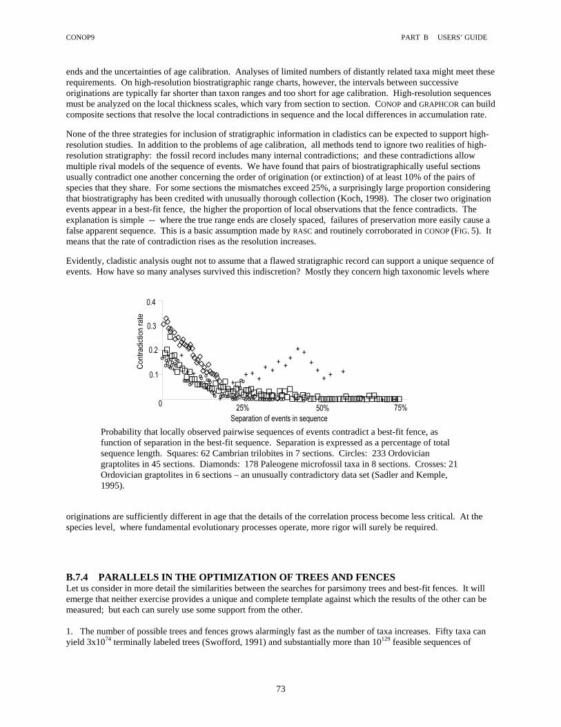
CONOP9 PART B USERS’ GUIDE

73

ends and the uncertainties of age calibration. Analyses of limited numbers of distantly related taxa might meet these requirements. On high-resolution biostratigraphic range charts, however, the intervals between successive originations are typically far shorter than taxon ranges and too short for age calibration. High-resolution sequences must be analyzed on the local thickness scales, which vary from section to section. CONOP and GRAPHCOR can build composite sections that resolve the local contradictions in sequence and the local differences in accumulation rate. None of the three strategies for inclusion of stratigraphic information in cladistics can be expected to support high-resolution studies. In addition to the problems of age calibration, all methods tend to ignore two realities of high-resolution stratigraphy: the fossil record includes many internal contradictions; and these contradictions allow multiple rival models of the sequence of events. We have found that pairs of biostratigraphically useful sections usually contradict one another concerning the order of origination (or extinction) of at least 10% of the pairs of species that they share. For some sections the mismatches exceed 25%, a surprisingly large proportion considering that biostratigraphy has been credited with unusually thorough collection (Koch, 1998). The closer two origination events appear in a best-fit fence, the higher the proportion of local observations that the fence contradicts. The explanation is simple -- where the true range ends are closely spaced, failures of preservation more easily cause a false apparent sequence. This is a basic assumption made by RASC and routinely corroborated in CONOP (FIG. 5). It means that the rate of contradiction rises as the resolution increases. Evidently, cladistic analysis ought not to assume that a flawed stratigraphic record can support a unique sequence of events. How have so many analyses survived this indiscretion? Mostly they concern high taxonomic levels where

originations are sufficiently different in age that the details of the correlation process become less critical. At the species level, where fundamental evolutionary processes operate, more rigor will surely be required. B.7.4 PARALLELS IN THE OPTIMIZATION OF TREES AND FENCES Let us consider in more detail the similarities between the searches for parsimony trees and best-fit fences. It will emerge that neither exercise provides a unique and complete template against which the results of the other can be measured; but each can surely use some support from the other. 1. The number of possible trees and fences grows alarmingly fast as the number of taxa increases. Fifty taxa can yield 3x1074 terminally labeled trees (Swofford, 1991) and substantially more than 10129 feasible sequences of

Probability that locally observed pairwise sequences of events contradict a best-fit fence, as function of separation in the best-fit sequence. Separation is expressed as a percentage of total sequence length. Squares: 62 Cambrian trilobites in 7 sections. Circles: 233 Ordovician graptolites in 45 sections. Diamonds: 178 Paleogene microfossil taxa in 8 sections. Crosses: 21 Ordovician graptolites in 6 sections – an unusually contradictory data set (Sadler and Kemple, 1995).

CONOP9 PART B USERS’ GUIDE

74

originations and extinctions (Kemple et al., 1995). It is not easy to accumulate sufficient characters and sections to prevent the number of equally good solutions from growing too. The tasks are “NP-complete” (Dell et al., 1992). 2. For both searches, a variety of constraints and objective functions may be used in different combinations (Swofford, 1998; Sadler, 1998, 1999). Each combination will likely yield a different solution; but that is the power of the approach -- an ability to explore the dependence of the outcome on a priori decisions about what is “best” and what is “simplest.” For correlation and for building trees from molecular data, there are also maximum likelihood formulations (Kemple, 1991; Nei, 1991; Huelsenbeck and Rannala, 1997); but they require extra assumptions and cannot build trees from morphologic data. 3. The outcome of both optimizations depends upon choices about the input criteria: which taxa to include; which characters or stratigraphic sections to include; and how to weight them. None of the weighting schemes are easy to justify. A priori decisions about the relative merits of different observations were essential to the original manual methods (Hennig, 1966; Shaw, 1964). Now, automation permits the simultaneous evaluation of so many observations that the total “weight of evidence” may replace the need for subjective weights on individual observations (Kemple et al., 1995). In both stratigraphy and cladistics, however, there are instances which prove that more evidence is not always better. 4. The true origination events are ordered and separated in time. Parsimony trees and best-fit sequences may both include measures of separation between events. But, in both cases, the relationship of these measures to time is as treacherous as it is enticing. Rigorous mathematical treatment of both problems has progressed by explicitly divorcing the spacing question from the sequencing question. The safest time scales are merely ordinal, not interval scales. The distance measures, whether rock thickness or character state changes, cannot be converted to time without radical simplifying assumptions that should not be allowed to distort the initial analysis. 5. The set of most-parsimonious trees can be rendered into a consensus tree. Branches in the consensus tree are common elements in all the equally most-parsimonious trees, they provide consensus sequences. Similarly, the set of best-fit fences contains a maximum consensus sequence -- the longest possible sequence constructed solely from events that appear in the same order in all rival fences. B.7.5 FUNDAMENTAL DIFFERENCES BETWEEN TREES AND FENCES It is technically possible to combine tree and fence building into one optimization, but there are significant differences that challenge the desirability of such full integration.

1. Parsimony trees minimize the number of implied homoplasies in the input character states -- a matter of interpretation of morphology. Best-fit fences minimize the implied local inadequacies of the fossil record -- a matter of fact rather than interpretation. Thus, the objective functions for parsimony trees and best-fit fences are conceptually different and measured in different units. Any combination of the two functions would inevitably weight one rather arbitrarily relative to the other.

2. With several different options for the objective functions and constraints for both trees and fences, the

number of possible combinations with different solutions is potentially overwhelming. (This is distinct from the choice of search strategies which influences the speed of the search, not the final outcome.)

3. The heuristics for searching among trees are not appropriate for fences. CONOP uses a nested optimization to

find the best-fit fence. The outer optimization searches among sequences and, for each trial sequence, the inner optimization solves the locating task to find the best-fit. Regardless of how the tree- and fence-building objective functions might be combined, the search for a joint best-sequence would require two inner optimizations -- one for the stratigraphic locating task and the other to find the most parsimonious tree.

4. Sequences are more completely resolved in fences than in trees; the sequence of events is fundamental to

correlation; and there is considerable merit to cladists’ arguments that the morphologic information used in

CONOP9 PART B USERS’ GUIDE

75

cladistic analysis is inherently more reliable than stratigraphic observations. All this indicates that it would be more beneficial to use cladistic insights in support of correlation than to include stratigraphic information in the search for parsimony trees.

5. The raw data for fence building are usually arrayed in a matrix of taxa and sections. Tree-building begins

with a matrix of taxa and characters. Thus, taxa appear to be the common component. Although traditional biostratigraphic correlation will find the sequence of originations for the taxa listed in the input matrix, cladistic analysis will not. The taxa used to build a tree are labels for a larger clade. The origination of the clade is not necessarily the origination of the taxon that labels the corresponding tip of the tree. Cladograms map the sequence of originations for the character states, not the label species. The only way to make both the tree-building and the fence-building exercises search for the same sequence is to base correlation on the appearance of character states rather than taxa. Although rarely undertaken, this tactic has been attractive to biostratigraphers for two other purposes: to gain more resolution where changes of character state outnumber the originations of new species; or to avoid taxonomic muddles caused by a web of morphological changes.

B.7.6 PROCEDURAL POSSIBILITIES Careful analysis of the temporal and geographic patterns of intraspecific variability will obviously improve the selection of character states for cladistic analysis. Now we have identified a bonus -- it permits correlation to be based on character states and become compatible with cladistic analysis, even at high resolution. Once correlation has been refocused from species to character states, there still remain several options to examine for integrating the stratigraphic and cladistic tasks. B.7.6.1 CORRELATION OF CHARACTER STATES AND TAXA First appearances of individual character states may be used in correlation just like the first appearance of species. Operationally, this requires extending the CONOP code to admit this new data type. The ranges of taxa represent the appearance and disappearance of sets of character states in single organisms. Because this is different from assembling the same set across two or more coexisting fossil species, it may be legitimate to compare taxon-based and character-based correlations and to array the originations of species and character states in the same sequence. Homoplasic character states are likely to accrue higher misfit penalties during correlation than non-homoplasic character states. So we should compare the worst-fit characters in the fences with the homoplasies identified by cladograms. In this fashion, the tree- and fence-building tasks may each be able to improve the selection (and/or weighting) of data for the other. B.7.6.2 INCORPORATING PARSIMONY TREES INTO CORRELATION PROBLEMS Fully pectinate branches pruned from parsimony trees may be treated as if they were additional stratigraphic sections. Each branch contributes its sequence of origination events and can be weighted according to cladistic measures of branch support and consistency. Character states whose relative age cannot be resolved, may be entered at the same level in the proxy section. Although these proxy sections introduce mixed-scales into the optimizations, we have already overcome a similar problem for an Ordovician time scale project that mixed thickness and time scales. Part of the solution is to measure stratigraphic adjustments and distances by counting event levels, not the distance between them. B.7.6.3 CONSENSUS SEQUENCES FROM TREES AND FENCES Joint optimization of trees and fences for the same set of character originations looks impractical. Nevertheless, the set of most-parsimonious trees and the set of best-fit fences can both be reduced to consensus sequences. We will seek ways to merge these into one consensus sequence.

CONOP9 PART B USERS’ GUIDE

76

B.7.6.4 INCORPORATING STRATIGRAPHIC SEQUENCES INTO CLADISTIC ANALYSIS Stratigraphic separation can be used, instead of absolute age separation, in the Manhattan strategy proposed by Siddall (1998). Representative composite sections, constructed by CONOP from the local section thicknesses, include estimates of the relative spacing of origination events. Alternatively, following the RASC strategy, the separation of individual origination events can be scaled as inversely proportional to the degree of local contradiction with the best-fit sequence. Because tree branches can be treated as stratigraphic sections, CONOP should be able to calculate the stratigraphic misfit for any tree and any single character state. This extends the options for measuring the consistency between a tree and a fence after the cladistic analysis has been completed independently. Unlike existing strategies, the new options can be applied to high-resolution studies.

CONOP9 PART C REFERENCE

77

C SUMMARY of FILES and SYNTAX C.1 THE CONOP PROGRAM FILES C.1.1 CONOP9.CFG The CONFIGURATION FILE: CONOP9.CFG is a text-file of user-editable run-time parameters for CONOP9.EXE. CONOP9.EXE solves a stratigraphic correlation problem based on the data in LOADFILE and writes answers to UNLOADMAIN, with or without UNLOADSECT, UNLOADEVNT and RUNLOGFILE, as instructed by CONOP9.CFG. CONOP9.CFG is also used by CONSORT9.EXE, which takes the preliminary PREPFILE listing and expands it by assigning the sequential numbers to collecting LEVELS, expanding top-only and bottom-only taxon entries, sorting the sequence of records, and writing the LOADFILE for CONOP9 to use. CONOP9.CFG is also used by CONTROL9.EXE, which examines all aspects of the LOADFILE data that do not require finding the best solution. LOAD THIS FILE (CONOP9.CFG) TO SAME DIRECTORY AS CONOP9.EXE, CONSORT9.EXE and CONTROL9.EXE. The name of this configuration file and the assumption that it resides with the EXE files is hard-coded into the EXE files. This condition cannot be altered except at source code level. Edit this file using any word processor that can save it as an ASCII text-file without formatting. Microsoft Word and WordPad are suitable. WordPad loads and unloads faster. Windows Notepad cannot edit the file unless it is shortened. Editing instructions are attached to the shipped version of the file. These instructions are reproduced in this guide and reference manual; so they may be deleted from CONOP9.CFG to shorten it considerably. C.1.2 CONOP9.EXE The MAIN EXECUTABLE FILE: CONOP9.EXE solves a stratigraphic correlation problem as instructed by parameter settings in CONOP9.CFG. It reads the raw stratigraphic data from the file identified by the LOADFILE parameter and any accompanying event and section dictionaries. It reports its solution and analysis to the file named in the UNLOADMAIN parameter, with or without additional reports as directed by the UNLOADSECT, UNLOADEVNT and RUNLOGFILE parameters in CONOP9.CFG. These are annotated text files suitable for word processing. CONOP9.EXE also writes a series of unannotated data files suitable for spreadsheet programs or other programs designed for numerical analysis. Some of these data files may be read by CONOP9.EXE to initialize subsequent runs. Others may be updated as a summary of multiple runs. LOAD THIS FILE (CONOP9.EXE) TO SAME DIRECTORY AS CONOP9.CFG. C.1.3 CONTROL9.EXE An AUXILLIARY EXECUTABLE FILE: CONTROL9.EXE examines (“trolls”) all aspects of the LOADFILE data that do not require finding the best solution. CONTROL9 has a run-time, drop down menu of options to analyze the input data set or map the penalty landscape. The CONTROL9 options fall into three categories: "standard," "advanced," and "experimental." Sadler uses the "experimental" options to map the problem landscape; they have very long run-times and are not at all user-friendly. LOAD THIS FILE (CONTROL9.EXE) TO SAME DIRECTORY AS CONOP9.CFG.

CONOP9 PART C REFERENCE

78

C.1.4 CONSORT9.EXE A second AUXILLIARY EXECUTABLE FILE: CONSORT9.EXE takes the preliminary PREPFILE listing and expands it by assigning the sequential numbers to collecting LEVELS, expanding top-only and bottom-only taxon entries, sorting the sequence of records, and writing the LOADFILE for CONOP9 to use. CONSORT9 also provides options to edit the weighting factors in LOADFILE. i.e. all input preparation. CONSORT9.EXE allows the stratigrapher to prepare a data file that does not meet all the rigors of the LOADFILE required by CONOP9.EXE. It is a preprocessor. Two particularly irksome requirements are dropped: the file identified by the PREPFILE parameter need not be sorted; and it is not necessary to assign sequential integers to the collecting horizons in each section. In the unsorted file, new records may be added to the end in any order. The addition of new finds from existing sections typically causes the horizon numbering to change – a very disagreeable editing chore. CONSORT9.EXE does not yet relax the requirement to give sections and taxa sequential integer codes with no gaps. Thus, sections and taxa cannot be so simply removed from the input files. The alternative is to weight them zero. CONSORT9.EXE provides the ability to change the weights for all records that pertain to a particular event, event type, taxon, or section. LOAD THIS FILE (CONSORT9.EXE) TO SAME DIRECTORY AS CONOP9.CFG. C.1.5 CONMAN9.EXE (STILL PRELIMINARY!!) A third AUXILLIARY EXECUTABLE FILE: CONMAN9.EXE is an attempt to provide a simple dedicated database manger, written in Visual Fortran. It is intended to guide the input and editing of range chart data, allow the selection of subsets of the sections and taxa for a CONOP9 run, and automate the preparation of CONOP9 input files. It is fully menu driven. It replaces almost all of the functions of CONSORT9, but it reads its own files as input, not the CONOP9 files that CONSORT9 expects. THIS FILE WAS FIRST SUBJECT TO BETA TESTING IN THE SUMMER OF 2004. Testing has been limited, but has led to a sequence of versions that contain small improvements. Guiding Principles:

1. The heart of the database should be a file for each stratigraphic section with dictionaries to translate entries in these files and tools for appending, editing, and exporting.

2. The database manager should have stand-alone capability in the sense that direct access to the raw files is not necessary.

3. Nevertheless, careful direct editing should be possible without hassle. The raw files should, therefore, be simple, header-free, sequential ASCII-files that can be edited with any basic text editor and produced by any spreadsheet or database program, if desired. The sequential attribute saves space and allows the program to read sequential or direct access files, provided t hat no field is left blank. The database manager should have the facility to append new records and edit old records. For safety, it should not delete records. “Bad” records may be edited/overwritten. Deletion of records would need to be accomplished outside the data manager.

4. The database manager should offer drop-down lists of dictionary entries for building the range-chart files. 5. The database manager should echo back all edited and appended records to the screen. 6. The raw files should contain a few redundant fields that improve readability. Therefore, in addition to the

taxon code numbers that relate the database files, there is a redundant field that can contain abbreviated taxon names.

Basic Rules:

1. The database contains the following dictionaries a. section dictionary

Contains the section names and the name of the corresponding file where the range chart data are located. Optional entries concern age and locations and sources. This dictionary must contain one record for every section in the database. Each record is a single line, ending in a carriage return. Section files that are not listed will be ignored (but not

CONOP9 PART C REFERENCE

79

erased). Section files will be read in the order of the lines in this dictionary; sort the dictionary lines if you wish to modify this order

b. taxon dictionary Contains one record for every taxon name used in any context in the database. The record must contain the taxon name, code and abbreviation. The taxon name is divided into genus, species, subspecies, and morphotype. Genus and species names are required; subspecies and morphotype are not. Unused subspecies and morphotype fields contain asterisks which the program reads as empty fields. In order to endure that the sorting functions operate properly, it is best to ensure that the code numbers are all of the same length by padding the numbers with leading zeroes (001, 002, . . . 009, 010, . . . 999) according to the size of the largest number. Optional entries concern author, year and synonyms. This dictionary must contain all taxon names used in range charts or synonymy, whether current or not, preferred or not. Each taxon in this may have one but only one preferred name listed

c. event dictionary Contains one record for every event other than a taxon range. The event code numbers should not duplicate taxon code numbers and should also be padded with leading zeroes to match the length of the largest number.

d. synonym dictionary Contains all the pairs of taxon names that have been linked by synonymy. Multiple synonyms may be entered for a single taxon by giving that taxon more than one record. But, only one of these synonyms may be operational in the taxon dictionary at any one time.

e. reference dictionary Contains one record for any reference or source. References are identified by a unique 8-character code. This code may be constructed from the first 4 letters in the authors name, followed by the last two digits of the year of publication and the last two digits of the first page (or total number of pages). This code is not constructed automatically or checked automatically, so any other unique assignment will suffice.

2. The database contains one file for every stratigraphic section. The section dictionary tracks which sections are in the database. Entries in the section files are translated by the other dictionaries.

3. Taxa are identified by name, code and abbreviation. The name follows rules of zoological nomenclature.

The code must be unique, but is otherwise unconstrained. The codes are sorted alphabetically, therefore, if a numerical sorting is desired they must carry sufficient leading zeroes to give all numbers the same number of digits. The abbreviation may be used for any second code, especially when taxa are imported from another database with its own preferred coding.

4. An asterisk is used for empty fields. CONMAN reads blank spaces as field separators, unless the blank is

enclosed within a phrase in inverted commas. An asterisk is used to indicate a field with missing information. Therefore, users should avoid asterisks and single inverted commas in all other situations.

5. CONMAN offers the following drop-down menus. Those in bold are essential; those in parentheses are

rudimentary or under construction. a. (BACK-UP for making backup files) b. (SETTINGS for changing the names and formats of input and output files ) c. GLOSSARY for displaying file contents d. PROOF for scanning files in search of inconsistent entries e. LIST/EDIT for listing files and editing the contents of their records f. APPEND for adding records to the dictionary files and section files g. SYNONYMY for managing the records of synonymous names

Synonyms are stored in two places. 1) For every name in the taxon dictionary, it is possible to enter a single name

as the currently preferred name; this is the active synonym; it must have its

CONOP9 PART C REFERENCE

80

own entry in the taxon dictionary. That is, the taxon dictionary includes active and obsolete names. Each obsolete name in the taxon dictionary may have only one active synonym (or none). The same active synonym may apply to more than one obsolete name. The synonym menu includes an option to automatically seek obsolete names in section files and replace them with the active name in the taxon dictionary.

2) There is also a synonym dictionary. Each record in the synonym dictionary has one active name, one obsolete name, and a reference code to identify the authority for that synonymy. There is no limit on the combinations of names in the synonym dictionary. Thus, when all record are taken together, one name may be listed with multiple obsolete names and the same obsolete name may appear in multiple records. The purpose of this dictionary is to record all known claims of synonymy, whether or not they are in use by the taxon dictionary.

h. EXPORT for building CONOP9 input files from the database files

The export process has the following steps: 1) select sections to be included; 2) select the taxa (paired events) to be included; 3) select other events (unpaired) to be included, if any; 4) build the CONOP9 input files; 5) edit the weighting of observed events in the input files, if desired.

It is neither necessary nor recommended to load this file (conman9.exe) to the same directory as conop9.cfg. It is recommended to keep this file in a separate directory with all the files that it reads and writes.

CONOP9 PART C REFERENCE

81

C.2 BEGINNER'S COMMAND SYNTAX The following provides instructions for a safe minimalist approach to editing CONOP9.CFG. All the commands are listed as in the configuration file, so that you can find them. Only the bold lines really need attention. Italics indicate safe items that you might as well edit for convenience. Annotations in parentheses suggest whether and when the other lines might be considered. Note these generalizations:

0. It is assumed that the problem is a correlation, not a seriation 1. It is assumed that the instance contains less than 20 sections and less than 100 taxa

If the instance is larger, increase the number of TRIALS. 2. Lines in bold face require planning; they must match your instance of the problem. 3. Items in italics are text strings that should be replaced with more meaningful entries. 4. Other command settings may be copied as is (without the trailing comments!). 5. File extension convention is not mandatory.

Files with .txt extension are annotated for reading in users’ word processor. Files with .dat extension are designed for loading FORTRAN arrays; explore with spreadsheet.

___________________ PROJECT= 'any old title will do' SECTIONS= number of sections in your input data (MUST BE CORRECT) TAXA= number of taxa in your input data (MUST BE CORRECT) EVENTS= number of other correlation events in your input dat (MUST BE CORRECT) MAX_LEVELS= 150 (need only be bigger than needed) MAX_LABELS= 15 (need only be bigger than needed) LOADFILE= ‘your path\your input data file name.dat’ (MUST BE CORRECT; default path is folder with

CONOP9.EXE) PREPFILE= ‘same as input file’ (no consequence for CONOP9.EXE) SECTFILE= ‘OFF’ (your section dictionary if available) SECTTAGFILE= 'OFF' (don't even think about it!) SECTTAGS = 'OFF' (don't even think about it!) LABELFILE= ‘OFF’ (your label dictionary; forget about it!) EVENTFILE= ‘OFF’ (your event dictionary if available) EVENTTAGFILE= 'OFF' (don't even think about it!) EVENTTAGS= 'OFF' (don't even think about it!) BESTKNOWN 0.0 (no consequence) ________________________ PENALTY= 'LEVEL' (an acceptable option for nearly all data sets) LETCONTRACT= 'OFF' (don't even think about it!) WEIGHTING= 'ON' (don't even think about it unless doing seriation!) USENEGATIVE= 'OFF' (all the other options are unsafe at any speed) NEARENOUGH= 0.0 (mostly harmless) EXCLUSIVES= 'no’ (don't even think about it!) FORCECOEX= 'SL’ ('SS' would not hurt) FORCEFb4L= 'ON' (‘OFF’ would not hurt) HOMERANGE= 'SL' ('SS' would not hurt) SMOOTHER= 0.0 (don't even think about it unless mimicking Shaw’s method) SQUEEZER= 0.0 (don't even think about it!) SHRINKER= 0.0 (don't even think about it!) TEASER= 0.0 (don't even think about it unless doing seriation!) STACKER= 'OFF' (don't even think about it unless doing seriation!) __________________________ SOLVER 'ANNEAL' (an almost universally appropriate option) STEPS= 500 (may need adjustment for more efficient solution) TRIALS= 200 (may need adjustment for more efficient solution)

CONOP9 PART C REFERENCE

82

STARTEMP= 100 (may need adjustment for more efficient solution) RATIO= 0.98 (may need adjustment for more efficient solution) HOODSIZE= 'BIG’ (an almost universally appropriate option) STARTYPE= 'RAND' (change to 'FILE' to continue last run) STARTSECT= 1 (ignore!) STARTEVENT= 1 (ignore!) SHOWMOVIES= 'CHT' (ignore!) TRAJECTORY= 'ALL' (ignore!) VIDEOMODE= 'SVGA' (ignore!) PAUSES= 'ON' (ignore for now) CURVFILE= 'OFFcurve.dat' (ignore for now) CRV2FILE= 'OFFcurve2.dat' (ignore for now) ________________ COLUMNS= 7 UNLOADMAIN= 'outmain.txt' (without path, CONOP writes to its own folder) FITS_OUT= 'ON' (get a full analysis of the solution) CNFG_OUT= 'ON' (get a full analysis of the solution) SEQN_OUT= 'ON' (get a full analysis of the solution) INCR_OUT= 'ON' (get a full analysis of the solution) LOC_OUT= 'ON' (get a full analysis of the solution) OBS_OUT= 'ON' (get a full analysis of the solution) COMP_OUT= 'ON' (get a full analysis of the solution) UNLOADSECT= 'outsect.txt' (without path, CONOP writes to its own folder) SECT_OUT= 'OFF' (otherwise, this may write a very big file) UNLOADEVNT= 'outevnt.txt' (without path, CONOP writes to its own folder) EVNT_OUT= 'OFF' (otherwise, this may write a very big file) COEX_OUT= 'OFF' (otherwise, this may write a very big file) CULLFILE= 'cull.dat (rarely needed) RUNLOGFILE= 'runlog.txt' (without path, CONOP writes to its own folder) SOLNLIST= 'OFF' (rarely needed) STARTFILE= 'soln.dat' (needed to continue the previous run) STEPFILE= 'OFF' (rarely needed) BESTARTFILE= 'bestsoln.dat' (might not be written) COMPOSFILE= 'cmpst.dat' (easier to read in outmain.txt) COMPOSNMBR= 0 (ignore) COMPOSTYPE= 'ZST' (other settings generally inferior) OBSDFILE= 'obsd.dat' (easier to read in outmain.txt) PLCDFILE= 'plcd.dat' (easier to read in outmain.txt) EXTNFILE= 'extn.dat' (easier to read in outmain.txt) COEXISTFILE= 'coex.dat' (only useful if restarting a very big data set) FAD_LADFILE= 'Fb4L.dat' (not essential) ORDERFILE= 'order.dat' (not needed)

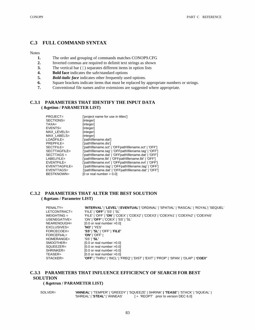
CONOP9 PART C REFERENCE

83

C.3 FULL COMMAND SYNTAX Notes

1. The order and grouping of commands matches CONOP9.CFG 2. Inverted commas are required to delimit text strings as shown 3. The vertical bar ( | ) separates different items in option lists 4. Bold face indicates the safe/standard options 5. Bold-italic face indicates other frequently used options. 6. Square brackets indicate items that must be replaced by appropriate numbers or strings. 7. Conventional file names and/or extensions are suggested where appropriate.

C.3.1 PARAMETERS THAT IDENTIFY THE INPUT DATA

( &getinn / PARAMETER LIST)

PROJECT= ['project name for use in titles'] SECTIONS= [integer] TAXA= [integer] EVENTS= [integer] MAX_LEVELS= [integer] MAX_LABELS= [integer] LOADFILE= ['path\filename.dat'] PREPFILE= ['path\filename.dis'] SECTFILE= ['path\filename.sct' | 'OFFpath\filename.sct' | 'OFF'] SECTTAGFILE= ['path\filename.tag' | 'OFFpath\filename.tag' | 'OFF'] SECTTAGS = ['path\filename.dat' | 'OFFpath\filename.dat' | 'OFF'] LABELFILE= ['path\filename.lbl' | 'OFFpath\filename.lbl’ | 'OFF'] EVENTFILE= ['path\filename.evt' | 'OFFpath\filename.evt' | 'OFF'] EVENTTAGFILE= ['path\filename.tag' | 'OFFpath\filename.tag' | 'OFF'] EVENTTAGS= ['path\filename.dat' | 'OFFpath\filename.dat’ | 'OFF'] BESTKNOWN= [0 or real number > 0.0]

C.3.2 PARAMETERS THAT ALTER THE BEST SOLUTION

( &getans / Parameter LIST)

PENALTY= 'INTERVAL' | 'LEVEL' |’EVENTUAL’| 'ORDINAL' | 'SPATIAL' | 'RASCAL' | ‘ROYAL’| ’SEQUEL’ LETCONTRACT= 'FILE' | 'OFF' | 'SS' | 'SL' WEIGHTING = 'FILE' | 'OFF' | 'ON' | 'COEX' | 'COEX2' | 'COEX3' | ‘COEX%1’ | ‘COEX%2’ | ‘COEX%5’ USENEGATIVE= 'ON' | 'OFF' | 'COEX' | 'SS' | 'SL' NEARENOUGH= [0.0 or real number >0.0] EXCLUSIVES= 'NO' | 'YES' FORCECOEX= 'SS' | 'SL' | 'OFF' | 'FILE' FORCEFb4L= 'ON' | 'OFF' | HOMERANGE= 'SS' | 'SL' SMOOTHER= [0.0 or real number >0.0] SQUEEZER= [0.0 or real number >0.0] SHRINKER= [0.0 or real number >0.0] TEASER= [0.0 or real number >0.0] STACKER= 'OFF' | 'THRU' | 'INCL' | 'FREQ' | 'DIST' | 'EXIT' | 'PROP' | ‘SPAN’ | 'OLAP' | ‘COEX’

C.3.3 PARAMETERS THAT INFLUENCE EFFICIENCY OF SEARCH FOR BEST

SOLUTION ( &getrun / PARAMETER LIST)

SOLVER= 'ANNEAL' | 'TEMPER' | 'GREEDY' | 'SQUEEZE' | SHRINK' | 'TEASE' | 'STACK' | 'SQUEAL' |

'SHREAL' | 'STEAL' | 'ANNEAS' [ + 'REOPT' prior to version DEC 6.0]

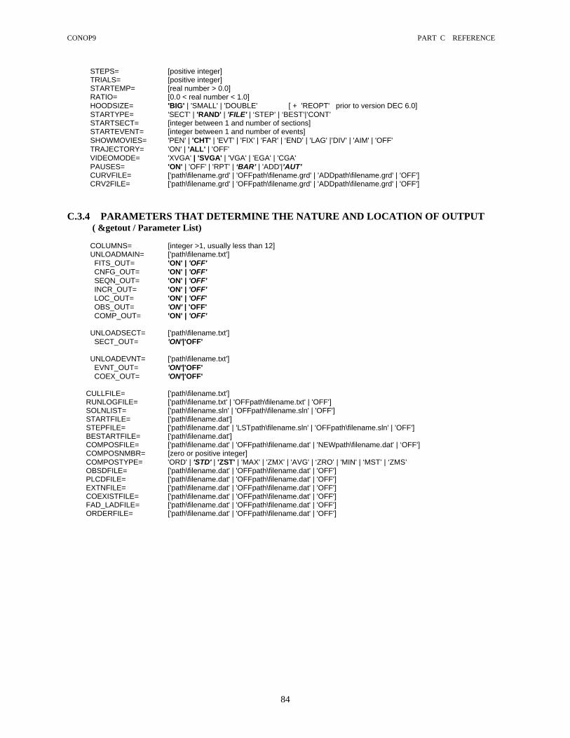
CONOP9 PART C REFERENCE

84

STEPS= [positive integer] TRIALS= [positive integer] STARTEMP= [real number > 0.0] RATIO= [0.0 < real number < 1.0] HOODSIZE= 'BIG' | 'SMALL' | 'DOUBLE' [ + 'REOPT' prior to version DEC 6.0] STARTYPE= 'SECT' | 'RAND' | 'FILE' | ‘STEP’ | ‘BEST’|’CONT’ STARTSECT= [integer between 1 and number of sections] STARTEVENT= [integer between 1 and number of events] SHOWMOVIES= 'PEN' | 'CHT' | 'EVT' | 'FIX' | 'FAR' | ‘END’ | 'LAG' |’DIV’ | 'AIM' | 'OFF' TRAJECTORY= 'ON' | 'ALL' | 'OFF' VIDEOMODE= 'XVGA' | 'SVGA' | 'VGA' | 'EGA' | 'CGA' PAUSES= 'ON' | 'OFF' | 'RPT' | ‘BAR’ | 'ADD'|’AUT’ CURVFILE= ['path\filename.grd' | 'OFFpath\filename.grd' | 'ADDpath\filename.grd' | 'OFF'] CRV2FILE= ['path\filename.grd' | 'OFFpath\filename.grd' | 'ADDpath\filename.grd' | 'OFF']

C.3.4 PARAMETERS THAT DETERMINE THE NATURE AND LOCATION OF OUTPUT

( &getout / Parameter List)

COLUMNS= [integer >1, usually less than 12] UNLOADMAIN= ['path\filename.txt'] FITS_OUT= 'ON' | 'OFF' CNFG_OUT= 'ON' | 'OFF' SEQN_OUT= 'ON' | 'OFF' INCR_OUT= 'ON' | 'OFF' LOC_OUT= 'ON' | 'OFF' OBS_OUT= 'ON' | 'OFF' COMP_OUT= 'ON' | 'OFF' UNLOADSECT= ['path\filename.txt'] SECT_OUT= 'ON'|'OFF' UNLOADEVNT= ['path\filename.txt'] EVNT_OUT= 'ON'|'OFF' COEX_OUT= 'ON'|'OFF'

CULLFILE= ['path\filename.txt'] RUNLOGFILE= ['path\filename.txt' | 'OFFpath\filename.txt' | 'OFF'] SOLNLIST= ['path\filename.sln' | 'OFFpath\filename.sln' | 'OFF'] STARTFILE= ['path\filename.dat'] STEPFILE= ['path\filename.dat' | 'LSTpath\filename.sln' | 'OFFpath\filename.sln' | 'OFF'] BESTARTFILE= ['path\filename.dat'] COMPOSFILE= ['path\filename.dat' | 'OFFpath\filename.dat' | 'NEWpath\filename.dat' | ‘OFF'] COMPOSNMBR= [zero or positive integer] COMPOSTYPE= 'ORD' | 'STD' | 'ZST' | 'MAX' | 'ZMX' | 'AVG' | ‘ZRO’ | 'MIN' | ‘MST’ | ‘ZMS’ OBSDFILE= ['path\filename.dat' | 'OFFpath\filename.dat' | 'OFF'] PLCDFILE= ['path\filename.dat' | 'OFFpath\filename.dat' | 'OFF'] EXTNFILE= ['path\filename.dat' | 'OFFpath\filename.dat' | 'OFF'] COEXISTFILE= ['path\filename.dat' | 'OFFpath\filename.dat' | 'OFF'] FAD_LADFILE= ['path\filename.dat' | 'OFFpath\filename.dat' | 'OFF'] ORDERFILE= ['path\filename.dat' | 'OFFpath\filename.dat' | 'OFF']

CONOP9 PART C REFERENCE

85

C.4 INPUT FILE FORMATS C.4.1 FORMAT FOR "LOADFILE" AND "PREPFILE" ASCII format; fields separated by blanks within records; records separated by a carriage return. Structure of fields and records is the same for LOADFILE and PREPFILE; but prepfile may be unsorted and levels need not be correct. C.4.1.1 SORTING “LOADFILE” MUST BE SORTED ON FIRST THREE FIELDS:

Primary Sort - field 1, event number, ascending Secondary Sort - field 2, event type, ascending Tertiary Sort - field 3, section number, ascending

"ascending" means first record (top of file) is event number 1 “PREPFILE” can be converted to LOADFILE format by running CONSORT9.EXE PREPFILE may eliminate the Level field or fill it with arbitrary integers. BUT, the sorting option in CONSORT9 must specify whether this field is present or not! C.4.1.2 RECORD STRUCTURE Each line in the file is considered a “record.” A record gives the level and weight for one event (e.g. FAD) as found in one section. Every record contains the same set of items, separated by blank spaces; each item is considered to be one “field” in the database record. The following field list is in the record order required for “PREPFILE” and “LOADFILE”: FIELD 1 Event Number

An integer that identifies the species or event These integers must be consecutive, starting with 1 (no gaps!)

FIELD 2 Event Type An integer code for the type of event

The following code numbers are defined for use or in development -3 unconstrained unpaired event [BOB] -2 unpaired disappearance event [DIS] -1 unpaired appearance event [APP] 0 spacer event (hiatus level) [GAP] under development 1 paired first appearance event [FAD] 2 paired last appearance event [LAD] 3 mid-range event [MID] 4 marker bed/event [ASH] 5 dated bed/event [AGE] 6 cycle boundary [CYC] under development

FIELD 3 Section Number

An integer corresponding to the section; sections must be numbered consecutively, starting with 1, and with no gaps!

FIELD 4 Horizon Position in stratigraphic distance from (arbitrary) base of section

An integer or decimal number (treated as decimal within the program) representing the stratigraphic position above the base of the section. Units of measurement are left to the user; because no unit conversion is made within the program, units are not needed.

CONOP9 PART C REFERENCE

86

The base of the section SHOULD NOT be 0.00. It may be positive or negative. Internally, the program resets all section bases to 1000.00 and uses zeros to indicate missing events. Thus, field 4 values of 0.00 will likely be converted to non-zero values. But, for safety and compatibility with earlier versions of CONOP, 0.00 values should still be avoided. For well depths, values must have a negative sign; thus, the real values still increase up section for purposes of internal arithmetic. The top of the well may be 0.0 as long as the top is not an event horizon. The top of the well may have positive elevation; but it is best that no event level correspond to zero elevation.

FIELD 5 Level

An integer corresponding to the rank position of the event horizon in local section. Level numbers begin with 1 for the lowest event horizon and increase consecutively upward. A given level always has the same horizon value in one section. Because this number is easily assigned by the database manager or spreadsheet used to store the raw stratigraphic data, CONOP9.EXE does not attempt this task. However, the field may be left as zeros (or any integers) or even eliminated if the program CONSORT9.EXE is run before CONOP9.EXE. That sorting run will supply a menu choice between files that contain a level field and files that do not. Earlier versions used -1 for events known to extend below section and -2 for events known to extend above; This convention has been dropped. All range-end events recorded at the top or bottom levels of a section are assumed to be truncations and do not accrue a penalty. If a taxon is known to exist below the measured section, assign its FAD to the base (level 1). If the taxon is known to occur above the measured section assign its LAD to the section top. Observe this convention regardless of the apparent range ends within the section in order to achieve better results in seriation problems

FIELD 6 Moves Permitted

Integer code for freedom of placement. The following codes are defined: 0 = does not move (e.g. Type 4, 5 events; ASH, AGE) 1 = may move down section only (e.g. Type 1, -1 events: FAD, APP) 2 = may move up section only (e.g. Type 2, -2 events: LAD, DIS) 3 = may move up or down (e.g. Type 3, -3 events: MID, BOB) Types 4, 5, and 6, which were reserved but not used in earlier versions have been abandoned. Their anticipated purpose in treating reworked and caved events has been treated differently.

FIELD 7 Weight Up

Decimal-valued relative weight for up-section range extension; Default value is 1.00; may be larger or smaller than 1; larger values imply better established local range; may be set to zero for LAD to eliminate influence of event on solution, except through coexistence table. FOR DATED HORIZONS, this is the younger end of the range of probable age; i.e. SMALLER number. For dates in different sections, it is used for partial ordering. It may be set equal to Weight-Down to indicate that the age is certain. A full range of menu-driven editing options for resetting the weights is provided by CONSORT9.EXE.

FIELD 8 Weight Down

Decimal-valued relative weight for down-section range extension. Default value is 1.00; may be larger or smaller than 1; larger values imply better established local range; may be set to zero for FAD to eliminate influence of event on solution, except through coexistence table.

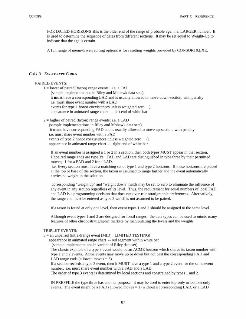
CONOP9 PART C REFERENCE

87

FOR DATED HORIZONS this is the older end of the range of probable age; i.e. LARGER number. It is used to determine the sequence of dates from different sections. It may be set equal to Weight-Up to indicate that the age is certain.

A full range of menu-driven editing options is for resetting weights provided by CONSORT9.EXE.

C.4.1.3 EVENT-TYPE CODES PAIRED EVENTS:

1 = lower of paired (taxon) range events; i.e. a FAD (sample implementations in Riley and Mohawk data sets) it must have a corresponding LAD and is usually allowed to move down-section, with penalty i.e. must share event number with a LAD events for type 1 honor coexistences unless weighted zero (1 appearance in animated range chart -- left end of white bar

2 = higher of paired (taxon) range events; i.e. a LAD

(sample implementations in Riley and Mohawk data sets) it must have corresponding FAD and is usually allowed to move up-section, with penalty i.e. must share event number with a FAD events of type 2 honor coexistences unless weighted zero (1 appearance in animated range chart -- right end of white bar

If an event number is assigned a 1 or 2 in a section, then both types MUST appear in that section. Unpaired range ends are type 3's. FAD and LAD are distinguished in type three by their permitted moves; 1 for a FAD and 2 for a LAD. i.e. Every section must have a matching set of type 1 and type 2 horizons. If these horizons are placed at the top or base of the section, the taxon is assumed to range farther and the event automatically carries no weight in the solution. corresponding "weight up" and "weight down" fields may be set to zero to eliminate the influence of any event in any section regardless of its level. Thus, the requirement for equal numbers of local FAD and LAD is a programming decision that does not over-rule stratigraphic preferences. Alternatively, the range end must be entered as type 3 which is not assumed to be paired. If a taxon is found at only one level, then event types 1 and 2 should be assigned to the same level. Although event types 1 and 2 are designed for fossil ranges, the data types can be used to mimic many features of other chronostratigraphic markers by manipulating the levels and the weights

TRIPLET EVENTS: 3 = an unpaired (intra-)range event (MID) LIMITED TESTING!!

appearance in animated range chart -- red segment within white bar (sample implementations in variant of Riley data set) The classic example of a type 3 event would be an ACME horizon which shares its taxon number with type 1 and 2 events. Acme events may move up or down but not past the corresponding FAD and LAD range ends (allowed moves = 3). If a section records a type 3 event, then it MUST have a type 1 and a type 2 event for the same event number. i.e. must share event number with a FAD and a LAD. The order of type 3 events is determined by local sections and constrained by types 1 and 2. IN PREPFILE the type three has another purpose: it may be used to enter top-only or bottom-only events. The event might be a FAD (allowed moves = 1) without a corresponding LAD, or a LAD

CONOP9 PART C REFERENCE

88

(allowed moves = 2) without the corresponding FAD. CONSORT9.EXE must be used to expand these types before running CONOP9EXE. The missing paired event is entered at the same level as the observed event, but weighted 0.1. Type 3 is altered to type 1 for FADs and type 2 for LADs.

UNPAIRED EVENTS: -1= an unpaired appearance event (APP); allowed to move down only

may be used for a FAD that lacks a reliable FAD designed for first appearance of character traits Type –1 events may not be mixed with FADs for same event number Type –1 events may not share event number with any other events

appearance in animated range chart -- yellow dash -2=an unpaired disappearance event (DIS); allowed to move up only

may be used for a LAD that lacks a reliable LAD designed for last appearance of character traits Type –2 events may not be mixed with LADs for same event number Type –2 events may not share event number with any other events

appearance in animated range chart -- yellow dash

-3=an unpaired unconstrained event; allowed to move up and down (BOB) may be used for any unconstrained event Type -3 events may not share event number with any other events

appearance in animated range chart -- yellow dash

4 = unique marker horizon (ASH); not allowed to move (sample implementations in Mohawk data set) Marker horizons may not be moved up- or down-section (allowed moves = 0). Their order is known only from the preservation sequence in local sections. They honor the order of superposition but do not play a role in coexistence. Type four events must be uniquely matched; i.e. every local observation of an event of type 4 with the same event number is assumed to be the same chronostratigraphic marker. The solution has no option but to correlate them. Type 4 events may not share event number with any other events

appearance in animated range chart -- yellow dash

5 = dated horizon (AGE); not allowed to move

(sample implementations in Mohawk data set) The order of dated horizons is known independently of local sections. The wtup and wtdown fields are used to record the range of possible age; e.g. plus and minus 2 sigma for a radiometric age determination. The dated horizons do not need to be found in more than one section to be useful; but there does need to be more than one dated horizon to influence the solution. Ordinarily, each dated horizon has a different event number. If the dated horizon is a marker bed known from more than one section, however, the same event number may be assigned in every section. Of course, the age range recorded in the weight fields should reflect the multiple age determinations.

Type 5 events do not move up or down section (allowed moves = 0), so the weight fields are not needed for their original purpose. Type 5 events may not share event number with any other events Type 5 events honors order of ages and superposition. They play no role in coexistence.

appearance in animated range chart -- yellow dash

CONOP9 PART C REFERENCE

89

6 = non-unique horizon (SEQ) NOT YET SUPPORTED; reserved for future development e.g. cycle or sequence boundary; undated polarity reversal Type 6 events will not move; they will be matched to any one of their kind. The weight fields will be used for parameters that determine the degree of match. appearance in animated range chart -- none

0 = hiatus (GAP) NOT YET SUPPORTED; reserved for future development

Hiatus horizons will not move. They will augment the penalty for range extensions and improve the translation from thickness to time.

appearance in animated range chart -- none C.4.1.4 ZERO WEIGHTS Both weight up and weight down may be set to zero for batches of locally observed events to eliminate the influence of a whole section or a whole taxon from the solution. This may be easier than re-numbering the taxa and/or sections to be consecutive from 1. Although the program has been made as robust as possible in the face of "zeroed out" sections and taxa, the stratigraphic consequences often require more careful analysis. Those taxa that are "zeroed out” of all sections may be placed almost anywhere in the final solution because their ranges can be extended without penalty! Events that are "zeroed out" are not used to fill out the coexistence matrix (a change from earlier versions of CONOP) and they have been eliminated from many of the graphical menu options. C.4.1.5 POSSIBLE COMBINATIONS OF TYPE AND MOVE TYPE - MOVE PURPOSE CODED? TESTED? NON-EVENTS (not in coexistence or partial ordering matrix)

0 - 0 spacers - add penalty for crossing No None PAIRED EVENTS/ENTRIES (in coexistence matrix):

1 - 1 reliable FAD with LAD(2,2) or LAD(2,3) Yes Many 1 - 3 caved FAD Part None 2 - 2 reliable LAD Yes Many 2 - 3 reworked LAD Part None

work-around forbidden combinations 1 - 0 perfect FAD! use very large weight 2 - 0 perfect LAD! use very large weight

"UNPAIRED" ENTRIES that will be converted to paired events (FAD and LAD together) by CONSORT9

3 - 2 unpaired reliable LAD Yes Some useful for coexistence matrix 3 - 1 unpaired reliable FAD Yes Some useful for coexistence matrix

UNPAIRED EVENTS/ENTRIES (in partial ordering matrix): taxon events:

-3 - 3 unconstrained BOB Part None -2 - 2 unpaired disappearance DIS Part None -1 - 1 unpaired appearance APP Part None 3 - 3 unpaired taxon event Yes None without limit within range

work-around forbidden combination 3 - 0 perfect acme horizon! use very large weight

CONOP9 PART C REFERENCE

90

other unpaired events: 4 - 0 unique marker horizons Yes Many e.g. volcanic ash, identified mag reversal 5 - 0 dated horizons Yes Some e.g. dated bed with known range of probable age 6 - 0 non-unique horizons No None e.g. cyclothem boundary; unidentified mag reversals

C.4.1.6 PERMITTED* COMBINATIONS FOR PAIRED EVENTS IN ONE SECTION *The following lists include coded and tested combinations as well as those that are not yet coded and/or tested! It scraps some plans for type 4 and 5 moves mentioned in earlier versions. The parentheses enclose the combinations of type and moves (Type, Moves)

FAD entry - permissible LAD entries (above) (1,1) - (2,2) or (2,3) (1,3) - (2,2) or (2,3) (3,1) - no entry [PREPFILE ONLY] LAD entry - permissible FAD entries (below) (2,2) - (1,1) or (1,3) (2,3) - (1,1) or (1,3) (3,2) - no entry [PREPFILE ONLY]

C.4.1.7 POSSIBLE TREATMENTS OF CAVED RANGES (“TOPS ONLY DATA”) The following table indicates that three different strategies are available and a fourth is planned:

1. Move caved event up to its lowest trustworthy level (e.g. side wall core) and weight it 1.00; the allowed moves will shift it down as necessary. In other words, deliberately shrink the range to its trustworthy minimum and rely upon the fact that CONOP is built to extend ranges. In an extreme case, the FAD and LAD might be recorded at the LAD level. This is not the same as the 2nd option because the weight is 1.00.

2. Move the caved event to the top of the range and weight it zero. This will eliminate the FAD from the solution process; it is an excessive reaction unless the FADs are unreliable in all sections. CONSORT9 will do this if the LAD is entered as an unpaired event in PREPFILE

3. Enter the LAD as an unpaired DIS event, if no reliable Fad is seen in any section 4. Allow the caved event to move up or down; i.e. allow selective range contraction and hope that all the

unreworked sections will correct a minority of reworked ranges (Type, Moves) and level placed: LEVEL: Highest Observed Lowest Reliable Lowest Observed paired events (2,2)wt1 (1,1)wt1 avoids problem " (2,2)wt1 (1,1)wt0 places ends together and

discounts FAD " (2,2)wt1 (1,3)wt1 adjusts FAD moves unpaired event (3,2)wt1 [PREPFILE ONLY] will place ends together and discount FAD

CONOP9 PART C REFERENCE

91

C.4.1.8 POSSIBLE TREATMENTS OF REWORKED RANGES (BASES ONLY DATA) The following table indicates that three different strategies are available and a fourth is planned:

1. Move reworked event down to its lowest trustworthy level and weight it 1.00; the allowed moves will shift it up as necessary.

2. Move the reworked event to the bottom of the range and weight it zero to eliminate it from the solutions process. Do this if there are no reliable observations of the LAD in any other section. CONSORT9 will do this if the FAD is entered as an unpaired event in PREPFILE

3. Enter the FAD as an unpaired APP, if no section has reliable LAD 4. Allow the caved event to move up or down; i.e. allow selective range contraction and hope that all the

unreworked sections will correct a minority of reworked ranges. (Type, Moves) and level placed LEVEL: Lowest Observed Highest Reliable Highest Observed paired event (1,1)wt1 (2,2)wt1 avoids problem! " (1,1)wt1 (2,2)wt0 places ends together and discounts

LAD " (1,1)wt1 (2,3)wt1 adjusts LAD moves unpaired event (3,1)wt1 [PREPFILE ONLY] CONOP9.CFG will place ends together and discount LAD C.4.1.9 POSSIBLE TREATMENTS OF CAVED-&-REWORKED RANGES The table below shows four strategies:

1. Shrink the observed range to its reliable minimum and weight the events 1.00. 2. Leave the range ends as observed and weight them 1.00, but allow them to move up or down section in order

to fit the more reliable information form other sections. This is pointless unless the unreliable ranges are a small minority of the data.

3. Leave the range ends as observed, allow them to move up or down section, and set the weights to zero so that these observations do not influence the solution process.

4. Enter the FAD and LAD as unpaired events that move up and down (-3,3) (Type, Moves) and level placed LEVEL: Highest-Obs'd Highest-Rel. Lowest-Rel. Lowest-Obs'd paired events (2,2)wt1 (1,1)wt1 " (2,3)wt1 (1,3)wt1 " (2,2)wt0 (1,1)wt0 C.4.2 FORMAT FOR "SECTFILE" ASCII format; fields separated by blanks within records; records separated by a carriage return. The first column is a sorted, unbroken set of section numbers that must match the numbers in LOADFILE. The third column sorts the same set of numbers into the order that the sections are to be plotted in fence diagrams. The second column is a 3-character nickname for fitting into tight spaces on graphics screens. The fourth column is the “full” name. The fifth column indicates whether (1) or not (0) the section should be used for the spacing task and construction of the composite section.

1 'Chi' 9 'Chilca Shale' 1 2 'Gyo' 7 'Gualcamayo R' 1 3 'Naz' 1 'Nazareno Ck' 1 4 'Sap' 2 'Sapito' 1 5 'Tuc' 3 'Tucunuco' 1

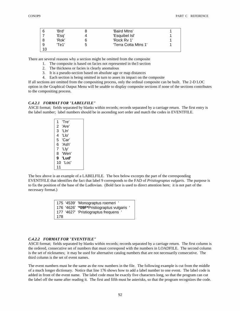
CONOP9 PART C REFERENCE

92

6 'Brd' 8 'Baird Mtns' 1 7 'Esq' 4 'Esquibel Isl' 1 8 'Rok' 6 'Rock Rv 1' 1 9 'Te1' 5 'Terra Cotta Mtns 1' 1 10

There are several reasons why a section might be omitted from the composite

1. The composite is based on facies not represented in the3 section 2. The thickness or facies is clearly anomalous 3. It is a pseudo-section based on absolute age or map distances 4. Each section is being omitted in turn to asses its impact on the composite

If all sections are omitted from the compositing process, only the ordinal composite can be built. The 2-D LOC option in the Graphical Output Menu will be unable to display composite sections if none of the sections contributes to the compositing process. C.4.2.1 FORMAT FOR "LABELFILE" ASCII format; fields separated by blanks within records; records separated by a carriage return. The first entry is the label number; label numbers should be in ascending sort order and match the codes in EVENTFILE.

1 'Tre' 2 'Are' 3 'Lln' 4 'Llo' 5 'Car' 6 'Ash' 7 'Lly' 8 'Wen' 9 'Lud' 10 'Loc' 11

The box above is an example of a LABELFILE. The box below excerpts the part of the corresponding EVENTFILE that identifies the fact that label 9 corresponds to the FAD of Pristiograptus vulgaris. The purpose is to fix the position of the base of the Ludlovian. (Bold face is used to direct attention here; it is not part of the necessary format.)

175 '4539' 'Monograptus roemeri ' 176 '4626' '*09F*Pristiograptus vulgaris ' 177 '4627' 'Pristiograptus frequens ' 178

C.4.2.2 FORMAT FOR "EVENTFILE" ASCII format; fields separated by blanks within records; records separated by a carriage return. The first column is the ordered, consecutive set of numbers that must correspond with the numbers in LOADFILE. The second column is the set of nicknames; it may be used for alternative catalog numbers that are not necessarily consecutive. The third column is the set of event names. The event numbers must be the same as the row numbers in the file. The following example is cut from the middle of a much longer dictionary. Notice that line 176 shows how to add a label number to one event. The label code is added in front of the event name. The label code must be exactly five characters long, so that the program can cut the label off the name after reading it. The first and fifth must be asterisks, so that the program recognizes the code.

CONOP9 PART C REFERENCE

93

The second and third characters are the label number -- with leading blanks as needed to make two characters. The fourth character is an ‘F’ if the label attaches to the FAD or an ‘L’ if the label attaches to the LAD. For attaching labels to unpaired events, use ‘X’ for marker bed events (type 4), ‘N’ for numerical age events (type 5), and ‘M’ for midrange events (type 3). The label marks an event that forms the BASE of a named stratigraphic unit. In some graphical output screens, these levels are marked within the composite sections and the label name is written on the UP-SECTION side.

167 '4499' 'Pristiograptus dubius parvus" ' 168 '4501' 'Gothograptus nassa ' 169 '4502' 'Colonograptus? praedeubeli ' 170 '4503' 'Colonograptus? deubeli ' 171 '4506' 'Neodiversograptus nilssoni ' 172 '4517' 'Bohemograptus bohemicus sl ' 173 '4518' 'Saetograptus fritsche linearis ' 174 '4521' 'Colonograptus colonus ' 175 '4539' 'Monograptus roemeri ' 176 '4626' '*09F*Pristiograptus vulgaris ' 177 '4627' 'Pristiograptus frequens ' 178 '4717' 'Pristiograptus pseudodubius ' 179 '4008' 'Araneograptus pulchellus ' 180 '4046' 'Kiaerograptus supremus ' 181 '4051' 'Tetragraptus phyllograptoides ' 182 '4092' 'Tetragraptus acclinans ' 183

The previous example used catalog numbers for the nickname. Abbreviated names are another possibility:

168 'Got.nass' 'Gothograptus nassa ' 169 'Col.prae' 'Colonograptus? praedeubeli ' 170 'Col?deub' 'Colonograptus? deubeli ' 171 'Neo.nils' 'Neodiversograptus nilssoni ' 172 'Boe.bohe' 'Bohemograptus bohemicus sl ' 173

Within the FORTRAN code and arrays, all events are assigned consecutive number. Paired events are numbered after unpaired events, with the FAD and LAD (+/-MID) assigned different numbers. Thus, the internal FORTRAN numbers reach higher values and do not correspond to any of the input numbers. Some of the CONOP9 output identifies these FORTRAN numbers. They are needed to predict the effect of the ‘STARTEVENT’ parameter.

CONOP9 PART C REFERENCE

94

D COMMAND REFERENCE See Part II See PART II under Reference9.doc or Reference9.pdf Prior to Version 6.4, the Users’ Guide and Reference were a single document.

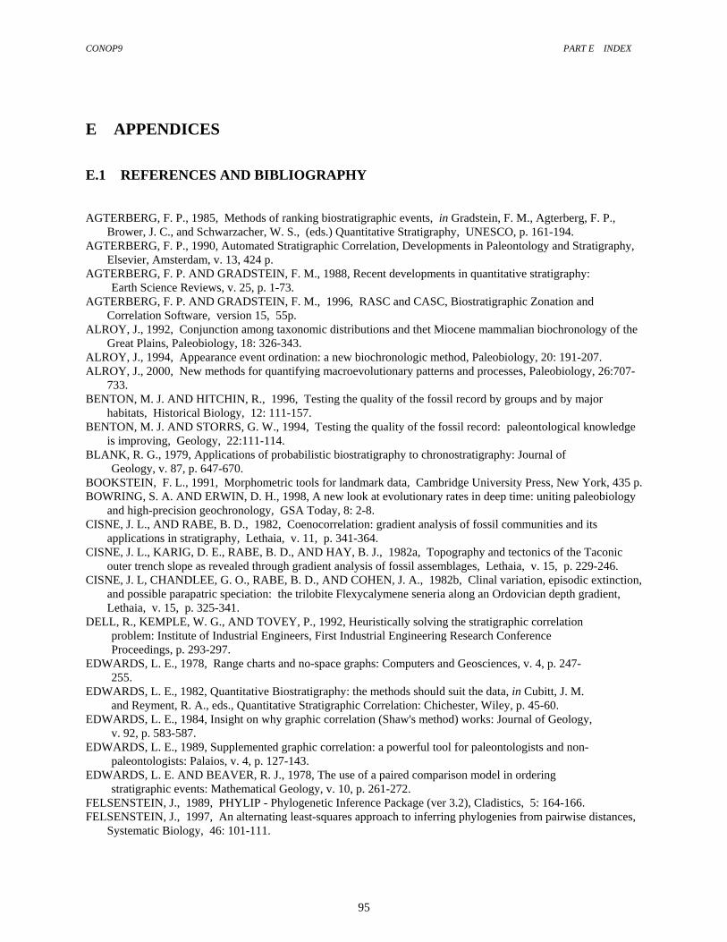
CONOP9 PART E INDEX

95

E APPENDICES E.1 REFERENCES AND BIBLIOGRAPHY AGTERBERG, F. P., 1985, Methods of ranking biostratigraphic events, in Gradstein, F. M., Agterberg, F. P.,

Brower, J. C., and Schwarzacher, W. S., (eds.) Quantitative Stratigraphy, UNESCO, p. 161-194. AGTERBERG, F. P., 1990, Automated Stratigraphic Correlation, Developments in Paleontology and Stratigraphy,

Elsevier, Amsterdam, v. 13, 424 p. AGTERBERG, F. P. AND GRADSTEIN, F. M., 1988, Recent developments in quantitative stratigraphy:

Earth Science Reviews, v. 25, p. 1-73. AGTERBERG, F. P. AND GRADSTEIN, F. M., 1996, RASC and CASC, Biostratigraphic Zonation and

Correlation Software, version 15, 55p. ALROY, J., 1992, Conjunction among taxonomic distributions and thet Miocene mammalian biochronology of the

Great Plains, Paleobiology, 18: 326-343. ALROY, J., 1994, Appearance event ordination: a new biochronologic method, Paleobiology, 20: 191-207. ALROY, J., 2000, New methods for quantifying macroevolutionary patterns and processes, Paleobiology, 26:707-

733. BENTON, M. J. AND HITCHIN, R., 1996, Testing the quality of the fossil record by groups and by major

habitats, Historical Biology, 12: 111-157. BENTON, M. J. AND STORRS, G. W., 1994, Testing the quality of the fossil record: paleontological knowledge

is improving, Geology, 22:111-114. BLANK, R. G., 1979, Applications of probabilistic biostratigraphy to chronostratigraphy: Journal of

Geology, v. 87, p. 647-670. BOOKSTEIN, F. L., 1991, Morphometric tools for landmark data, Cambridge University Press, New York, 435 p. BOWRING, S. A. AND ERWIN, D. H., 1998, A new look at evolutionary rates in deep time: uniting paleobiology

and high-precision geochronology, GSA Today, 8: 2-8. CISNE, J. L., AND RABE, B. D., 1982, Coenocorrelation: gradient analysis of fossil communities and its

applications in stratigraphy, Lethaia, v. 11, p. 341-364. CISNE, J. L., KARIG, D. E., RABE, B. D., AND HAY, B. J., 1982a, Topography and tectonics of the Taconic

outer trench slope as revealed through gradient analysis of fossil assemblages, Lethaia, v. 15, p. 229-246. CISNE, J. L, CHANDLEE, G. O., RABE, B. D., AND COHEN, J. A., 1982b, Clinal variation, episodic extinction,

and possible parapatric speciation: the trilobite Flexycalymene seneria along an Ordovician depth gradient, Lethaia, v. 15, p. 325-341.

DELL, R., KEMPLE, W. G., AND TOVEY, P., 1992, Heuristically solving the stratigraphic correlation problem: Institute of Industrial Engineers, First Industrial Engineering Research Conference Proceedings, p. 293-297.

EDWARDS, L. E., 1978, Range charts and no-space graphs: Computers and Geosciences, v. 4, p. 247-255.

EDWARDS, L. E., 1982, Quantitative Biostratigraphy: the methods should suit the data, in Cubitt, J. M. and Reyment, R. A., eds., Quantitative Stratigraphic Correlation: Chichester, Wiley, p. 45-60.

EDWARDS, L. E., 1984, Insight on why graphic correlation (Shaw's method) works: Journal of Geology, v. 92, p. 583-587.

EDWARDS, L. E., 1989, Supplemented graphic correlation: a powerful tool for paleontologists and non-paleontologists: Palaios, v. 4, p. 127-143.

EDWARDS, L. E. AND BEAVER, R. J., 1978, The use of a paired comparison model in ordering stratigraphic events: Mathematical Geology, v. 10, p. 261-272.

FELSENSTEIN, J., 1989, PHYLIP - Phylogenetic Inference Package (ver 3.2), Cladistics, 5: 164-166. FELSENSTEIN, J., 1997, An alternating least-squares approach to inferring phylogenies from pairwise distances,

Systematic Biology, 46: 101-111.

CONOP9 PART E INDEX

96

FISCHER, D. C., 1991, Phylogenetic analysis and it implications in evolutionary paleobiology, in Gilinsky, N. L. and Signor P. W. (eds.), Analytical Paleobiology, Paleontological Society Short Courses in Paleontology, 3: 103-122.

FISCHER, D. C., 1992, Stratigraphic parsimony, in Madison W. P. and Madison D. R., MacClade: analysis of phylogeny and character evolution, version 3, Sinauer Associates Inc., Sunderland, Mass., 124-129.

FISCHER, D. C., 1994, Stratocladistics: morphological and temporal patterns and their relation to phylogenetic process, in Grande, L. and Rieppel, O., (eds.), Interpreting the hierarchy of nature, p. 133-171, Academic Press, New York.

FOOTE, M., 1991, Morphologic patterns of diversification: examples from trilobites, Palaeontology, 34: 461-485. FOOTE, M., 1993, Discordance and concordance between morphological and taxonomic diversity, paleobiology,

19: 185-204. FOOTE, M., 1996, On the probability of ancestors in the fossil record, Paleobiology, 22: 141-151. FOOTE, M., HUNTER, J. P., CHRISTINE, M. J., SEPKOSKI, J. J., 1999, Evolutionary and preservational

constraints on the origins of biologic groups: divergence times of eutherian mammals, Science, 283: 1310-1314.

FOSTER, N. H., 1966, Stratigraphic leak: American Association of Petroleum Geologists Bulletin, v. 50, p. 2604-2606.

GAUTHIER, J., KLUGE, A. G., AND ROWE, T., 1988, Amniote phylogeny and the importance of fossils, Cladistics, 4: 105-209.

GEMAN, S. AND GEMAN, D., 1984, Stochastic relaxation, Gibbs distributions, and the Bayesian restoration of images: Institute of Electrical and Electronics Engineers Transactions on Pattern Analysis and Machine Intelligence, v. 6, p. 721-741.

GLOVER, F., 1990, Tabu search: a tutorial: Boulder, Author's Course Notes, University of Colorado, 47 p.

GOLDMAN, D., MITCHELL, C. E., BERGSTROM, S. G., DELANO, J. W., AND TICE, S. T., 1994, K-bentonites and graptolite stratigraphy in the Middle Ordovician of New York State and Quebec: a new chronostratigraphic model, Palaios, v. 9, p. 124-143.

GRADSTEIN, F. M., AGTERBERG, F. P., BROWER, J. C., AND SCHWARZACHER, W. S., 1985, Quantitative Stratigraphy: Dordrecht, UNESCO, Reidel Publishing Company, 598 p.

GRADSTEIN, F. M., 1987, Four quantitative stratigraphic methods: Ouro Preto, Proceedings of the 4th Cogeodata Symposium, p. 67-82.

GUEX, J., 1977, Une nouvelle méthod d'analyse biochronologique; note preliminaire: Laboratoire de Géologie, Mineralogie, Geophysique et Mussée Géologique de l'Université de Lausanne Bullétin, v. 224, p. 309-321.

GUEX, J., 1991, Biochronological Correlations: Berlin, Springer Verlag, 252 p. HAMMERSLEY, J. M. AND HANDSCOMB, D. C., 1964, Monte Carlo Methods: London, Methuen, 169

p. HAY, W. W., 1972, Probabilistic stratigraphy: Eclogae Geologica Helvetica, v. 65, p. 255-266. HENNIG, W., 1966, Phylogenetic Systematics, University of Illinois Press, Urbana, 263 p. HITCHIN, R., AND BENTON, M. J., 1997, Congruence between parsimony and stratigraphy: comparison of

three indices, Paleobiology, 23: 20-32. HITCHIN, R., AND BENTON, M. J., 1997, Stratigraphic indices and tree balance, Systematic Biology, 46: 563-

569. HOOD, K. C., 1986, GraphCor, interactive graphic correlation for microcomputers, version 2.2, K. C. Hood,

Houston. HOOD, K. C., 1995, Evaluating the use of average composite sections and derived correlations in the graphic

correlation technique, in Mann, K. O. and Lane, H. R., (eds.), Graphic Correlation, SEPM Special Publication, v. 53, p. 83-93.

HUELSENBECK, J. P., 1994, Comparing the stratigraphic record to estimates of phylogeny, Paleobiology, 20: 470-483.

HUELSENBECK, J. P. AND RANNALA, B., 1997, Maximum likelihood estimation of topology and node times using stratigraphic data, Paleobiology, 23: 174-180.

JONES, D. J., 1958, Displacement of microfossils: Journal of Sedimentary Petrology, v. 24, p. 453-467. KENDALL, M. G., 1975, Rank Correlation Methods: London, Griffin, 202 p.

CONOP9 PART E INDEX

97

KEMPLE, W. G., 1991, Stratigraphic correlation as a constrained optimization problem: Unpublished PhD dissertation, University of California, Riverside, 189 p.

KEMPLE, W. G., SADLER, P. M., AND STRAUSS, D. J., 1989, A prototype constrained optimization solution to the time correlation problem, in Agterberg, F. P. and Bonham-Carter, G. F., eds., Statistical Applications in the Earth Sciences: Ottawa, Geological Survey of Canada, Paper 89-9, p. 417-425.

KEMPLE, W. G., SADLER, P. M. AND STRAUSS, D. J., 1995, Extending graphic correlation to many dimensions: stratigraphic correlation as constrained optimization, in Mann, K. O. and Lane, H. R., (eds.), Graphic Correlation, SEPM Special Publication, v. 53, p. 65-82.

KIRKPATRICK, S., GELATT, C. D., AND VECCHI, M. P., 1983, Optimization by simulated annealing: Science, v. 220, p. 671-680.

KOCH, C. F., 1998, ‘Taxonomic barriers’ and other distortions within the fossil record, in Donovan, S. K., and Paul, C. R. C. (eds.), The adequacy of the fossil record, Wiley, New York, p. 189-206.

LAPOINTE, F.-J. AND CUCUMEL, G., 1997, The average consensus procedure: contribution of weighted trees containing identical or overlapping sets of taxa, Systematic Biology, 46: 306-312.

LIEBERMANN, B. S., 1997, Early Cambrian paleogeography and tectonic history: a biogeographic approach, Geology, 25: 1039-1042.

LIEBERMANN, B. S., 1998, Cladistic analysis of the early Cambrian olenelloid trilobites, Journal of Paleontology, 72: 59-78.

LIEBERMANN, B. S., 1999, Testing the Darwinian legacy of the Cambrian radiation using trilobite phylogeny and biogeography, Journal of Paleontology, 73: 176-181.

MARSHALL, C. R., 1990, Confidence intervals on stratigraphic ranges: Paleobiology, v. 16, p. 1-10. MARSHALL, C. R., 1998, Determining stratigraphic ranges, in Donovan, S. K., and Paul, C. R. C. (eds.), The

adequacy of the fossil record, Wiley, New York, p. 23-53. MACLEOD, N. AND SADLER, P. M., 1995, Estimating the line of correlation, in Mann, K. O. and Lane, H. R.,

(eds.), Graphic Correlation, SEPM Special Publication, v. 53, p. 51-64. METROPOLIS, N., ROSENBLUTH, A. W., ROSENBLUTH, M. N., TELLER, A. H., AND TELLER, E.,

1953, Equation of state calculations by fast computing machines: Journal of Chemical Physics, v. 21, p. 1087-1092.

MILLER, F. X., 1977, The graphic correlation method in biostratigraphy, in Kauffman, E. G. and Hazel, J. E., eds., Concepts and methods of biostratigraphy: Stroudsberg, Dowden, Hutchinson and Ross, p. 165-186.

NEI, M., 1991, Relative efficiencies of different tree-making methods for molecular data, in Miyamoto, M. M. and Cracraft, J., (eds.) Phylogenetic analysis of DNA sequences, Oxford University Press, p. 90-128.

NORELL, M. A., 1992, Taxic origin and temporal diversity: the effect of phylogeny, in Novacek, M. J., and Wheeler, Q. D. (eds.), Extinction and Phylogeny, Columbia University Press, New York, p. 89-118.

NORELL, M. A. AND NOVACEK, M. J., 1992, The fossil record and evolution: comparing cladistic and paleontologic evidence for vertebrate history, Science, 255: 1690-1693.

PALMER, A. R., 1954, The faunas of the Riley Formation in Central Texas: Journal of Paleontology, v. 28, p. 709-786.

PISIAS, N. G., BARRON, J. A., NIGRINI, C. A., AND DUNN, D. A., 1985, Stratigraphic resolution of leg 85 drill sites: an initial analysis, in Mayer, L., Thayer, F., and others, eds., Initial Reports of the Deep Sea Drilling Project, v. 85, p. 695-708.

PLATNICK, N. I., 1989, An empirical comparison of microcomputer parsimony programs, II, Cladistics, 5: 145-162.Ramsköld, L., and Edgecombe, G. E. 1991, Trilobite morphology revisited, Historical Biology, 4: 267-283.

REMANE, J., 1985, Der Artbegriff in Zoologie, Phylogenetik und Biostratigraphie, Paläontologische Zeitschrift, 59: 171-182.

RUBEL, M., 1978, Principles of construction and use of biostratigraphic scales for correlation: Computers and Geoscience, v. 10, p. 97-105.

SADLER, P. M. 1998, Biostratigraphic correlation as constrained optimization, in Crampton, J. and Cooper, R., (eds.) Integrated stratigraphy, new dimensions, New Zealand Institute of Geological and Nuclear Sciences, p. 34-39.

SADLER, P. M. AND KEMPLE, W. G., 1995, Using rapid, multidimensional, graphic correlation to evaluate chronostratigraphic models for the Mid-Ordovician of the Mohawk Valley, New York, in Cooper, J. D.,

CONOP9 PART E INDEX

98

Droser, M. L., and Finney, S. C. (eds.), Short Papers for the Seventh International Symposium on the Ordovician System, SEPM Pacific Section Books, v. 77, p. 257-260.

SADLER, P. M. AND STRAUSS, D. J., 1990, Estimation of completeness of stratigraphical sections using empirical data and theoretical models, Journal of the Geological Society of London, 147: 471-485.

SHAW, A. B., 1964, Time in stratigraphy: New York, McGraw Hill, 365 p. SIDDALL, M. E., 1995, Stratigraphic consistency and the shape of things, Systematic Biology, 45: 111-115. SIDDALL, M. E., 1998, Stratigraphic fit to phylogenies: a proposed solution, Cladistics, 14: 201-208. SMITH, A. B. AND LITTLEWOOD, D. J. T., 1994, Paleontological data and molecular phylogenetic analysis,

Paleobiology, 20: 259-273. SMITH, L. H., 1998, Species level phenotypic variation in lower Paleozoic trilobites, Paleobiology, 24: 17-36. STRAUSS, D. J. AND SADLER, P. M., 1989, Classical confidence intervals and the Bayesian probability

estimates for ends of local taxon ranges: Mathematical Geology, v. 21, p. 411-427. SWIDERSKI, D. L., ZELDITCH, M. L., AND FINK, W. L., 1998, Why morphometrics is not special: coding

quantitative data for phylogenetic analysis, Systematic Biology, 47: 508-519. SWOFFORD, D. L., 1991, PAUP. Phylogenetic analysis using parsimony, version 3.0, Illinois Natural History

Survey. SWOFFORD, D. L., 1998, PAUP*. Phylogenetic analysis using parsimony (* and other methods),

version 4., Sinauer Associates, Sunderland, Massachusetts. TIPPER, J. C., 1988, Techniques for quantitative stratigraphic correlation: a review and annotated

bibliography: Geological Magazine, v. 125, p. 475-494. VAIL, P. R., MITCHUM, R. M. Jr., AND THOMPSON, S., 1977, Global cycles of relative changes in sea

level, in Payton, C. E., ed., Seismic stratigraphy - Applications to Hydrocarbon Exploration: Tulsa, American Association of Petroleum Geologists Memoir 26, p. 83-98.

WAGNER, P. J., 1995, Stratigraphic tests of cladistic hypotheses, Paleobiology, 21: 153-178. WAGNER, P. J., 1998, Phylogenetic analyses and the quality of the fossil record, in Donovan, S. K., and

Paul, C. R. C. (eds.), The adequacy of the fossil record, Wiley, New York, p. 165-187. WILSON, L. R., 1964, Recycling, stratigraphic leakage, and faulty techniques in palynology: Grana

Palynologica, v. 5, p. 427-436. ZELDITCH, M. L., FINK, W. L., AND SWIDERSKI, D. L., 1995, Morphometrics, homology, and phylogenetics,

quantified characters as synapomorphies, Systematic Biology, 44: 179-189.

CONOP9 PART E INDEX

99

F INDEX Items in UPPER CASE (except for standard abbreviations) are CONOP parameter names or CONOP parameter options or file names.

& &GETANS, 12, 83 &GETINN, 11, 83 &GETOUT, 11, 44, 84 &GETRUN, 12, 83

A Accumulation Rate, 21, 25, 27, 47, 48, 73 Animated Range Chart, 12, 13, 14, 39, 44, 50, 51, 54, 59,

87, 88, 89 ANNEAL, 12, 37, 57, 81, 84 Aqueduct Analogy, 24, 25 ASCII, 11, 77, 85, 91, 92

B Back-up, 38 Base of Section, 85 Best Fit, 13, 17, 19, 33, 34, 36, 37, 42, 44, 45, 52, 60, 61,

62, 66, 67, 72, 73, 74, 75, 76 Best Fit Interval, 17, 61 BESTARTFILE, 12, 45, 52, 82, 84 BESTKNOWN, 81, 83 Boltzmann, 16, 53, 55

C Cambrian, 9, 11, 34, 38, 97 Caved Ranges, 90, 91 CGA, 84 Cladistics, 70, 71, 72, 73, 74, 75, 76, 95, 96, 97, 98 Cladogram, 52, 70 CNFG_OUT, 44, 82, 84 COEX_OUT, 44, 82, 84 Coexistence, 16, 21, 25, 30, 33, 34, 35, 36, 38, 44, 45, 49,

50, 52, 58, 86, 87, 88, 89 Coexistence Matrix, 35, 38, 45, 58, 86, 89 COEXISTFILE, 12, 45, 82, 84 COLUMNS, 44, 82, 84 COMP_OUT, 44, 82, 84 COMPOSFILE, 12, 45, 82, 84 Composite Section, 22, 23, 35, 39, 41, 45, 47, 48, 73, 75,

91, 93, 96 COMPOSNMBR, 82, 84 COMPOSTYPE, 82, 84 Conodonts, 63

CONOP9.CFG, 8, 9, 11, 34, 44, 50, 52, 77, 78, 80, 81, 83, 91

CONOP9.EXE, 8, 11, 12, 77, 78, 81, 86 CONSORT9.EXE, 8, 77, 78, 80, 85, 86, 87, 88 Constraint, 19, 22, 23, 24, 25, 32, 35, 52 Constraint - mandatory, 25 Constraint - optional, 19, 22, 23, 24, 25, 32, 35, 52 Constraints, 19, 20, 21, 25, 29, 40, 45, 48, 50, 52, 72, 74,

96 CONTROL9.EXE, 8, 77 Cooling Schedule, 45, 50, 54, 55, 56, 59, 60, 61, 63 CRV2FILE, 11, 82, 84 CULLFILE, 11, 45, 82, 84 CURVFILE, 11, 45, 82, 84

D Deep Sea Drilling Project, 23, 48, 97 Diversity, 12, 15, 35, 96, 97

E Economy of Fit, 24, 25, 26, 46, 49 Event Dictionary, 8, 9, 81 Event Number, 38, 85 Event Type, 38, 85 EVENTFILE, 11, 39, 50, 81, 83, 92 EVENTS, 11, 50, 51, 58, 81, 83, 87, 88, 89, 90 Evidence – negative, 15, 18, 29, 30 Evidence – positive, 18, 29, 30, 31 EVNT_OUT, 44, 82, 84 Exit, 12, 39 Extinction, 20, 23, 70, 73, 95 EXTNFILE, 12, 45, 82, 84

F FAD, 61, 85, 86, 87, 88, 89, 90, 91 Fences – best fit, 72, 73, 74, 75 First Appearance Datum (FAD), 13, 14, 29, 33, 35, 41, 50,

61, 85, 86, 87, 88, 89, 90, 91, 92, 93 FITS_OUT, 44, 82, 84 Font, 11 FORCECOEX, 12, 25, 45, 46, 81, 83

G Gaps, 29, 32, 33, 34, 70, 72, 78, 85 Genetic Algorithms, 61 Ghost Taxa, 72

CONOP9 PART E INDEX

100

GRAPHCOR, 73 Graphic Correlation, 4, 18, 22, 23, 24, 33, 38, 46, 47, 48,

95, 96, 97 Graptolites, 9, 63 GREEDY, 37, 59, 61, 84 Greedy Algorithm, 37, 60, 61

H Heuristic, 14, 16, 37, 53, 59, 60, 71 Hiatus, 21, 27, 41, 85, 89 HOMERANGE, 12, 29, 81, 83 HOODSIZE, 12, 54, 82, 84 Horizon Value, 85

I INCL, 30, 31, 58, 83 INCR_OUT, 44, 82, 84 INTERVAL, 12, 20, 27, 28, 30, 31, 37, 46, 47, 48, 49, 58,

60, 83

L LAD, 61, 86, 87, 88, 89, 90, 91 Last Appearance Datum (LAD), 13, 14, 29, 33, 35, 41, 50,

61, 85, 86, 87, 88, 89, 90, 91, 93 LETCONTRACT, 12, 25, 32, 81, 83 LEVEL, 20, 27, 30, 31, 37, 46, 58, 81, 83, 90, 91 Line of Correlation, 16, 20, 21, 22, 23, 24, 31, 32, 44, 45,

48, 62, 82, 84, 97 LOADFILE, 11, 38, 39, 77, 78, 81, 83, 85, 91, 92 LOC_OUT, 44, 82, 84 Locating Task, 18, 20, 25, 28, 30, 45, 74 Loop, 58

M MacCLADE, 72, 96 Magnetostratigraphy, 15, 23 Marker Beds, 14, 22, 23, 85, 88 Menu, 12, 14, 37, 39, 44, 45, 49, 77, 86, 87, 89 Metropolis Algorithm, 53 Minimum - global, 54, 55, 62, 66, 67, 68 Minimum – local, 53, 60, 61, 67, 68 Misfit, 13, 14, 15, 16, 17, 19, 20, 21, 22, 23, 24, 25, 26, 28,

29, 30, 31, 32, 33, 34, 35, 36, 37, 38, 45, 46, 52, 53, 54, 59, 60, 63, 66, 67, 68, 72, 75, 76

Misfit - interval, 13, 26, 63 Misfit - ordinal, 26 Mohawk Valley, 9, 14, 35, 46, 48, 63, 67, 68, 87, 88, 97 Moves – allowed, 38 Moves – permitted, 86

N Neighborhood, 52, 53, 54, 55, 60, 61 Neighborhood - big, 54, 57, 82, 84 Neighborhood - double, 54, 84 Neighborhood - small, 54, 57, 84

Non-Polynomial Complete, 15, 52, 53, 74 No-Space Graphs, 95

O Objective Function, 18, 32, 71, 74 OBS_OUT, 44, 82, 84 OBSDFILE, 12, 45, 82, 84 OLAP, 12, 30, 58, 83 Operations Research, 18, 37, 59 Optimization, 18, 19, 20, 24, 26, 28, 31, 32, 33, 38, 46, 47,

52, 53, 70, 72, 73, 74, 75, 96, 97 Optimization - constrained, 18, 19, 24, 46, 47, 71, 96, 97 Optimization – inner, 20, 74 Optimization – outer, 20, 53, 61, 74 ORDERFILE, 12, 45, 82, 84 ORDINAL, 20, 26, 37, 46, 58, 83 Ordovician, 9, 63, 75, 95, 96, 97 Origination, 20, 70, 71, 72, 73, 74, 75

P Pairwise Contradictions, 26, 37, 49 Parsimony, 72, 73, 74, 75, 96, 97, 98 Partial Reoptimization - full, 54, 57 Partial Reoptimization - partial, 54, 57 PAUP, 72, 98 PAUSES, 12, 14, 44, 50, 55, 59, 60, 82, 84 Pectinate, 71, 72, 75 PENALTY, 12, 20, 26, 27, 28, 37, 46, 60, 81, 83 Penalty - best, 61 PHYLIP, 72, 95 PLCDFILE, 12, 45, 82, 84 PREPFILE, 39, 77, 78, 81, 83, 85, 88, 90, 91, 92 PROJECT, 81, 83

R Radiometric Dates, 14, 15, 22, 23, 63, 85, 86, 88, 90 RAND, 12, 46, 52, 82, 84 Range Chart, 4, 9, 13, 14, 15, 24, 26, 32, 39, 40, 42, 43, 46,

49, 54, 71, 73, 95 Range Contraction, 20, 25, 26, 32, 90, 91 Range Extension, 20, 24, 32, 34, 35, 36, 38, 40, 42, 45, 86,

89 RASC, 15, 18, 26, 28, 29, 34, 37, 48, 95 RASCAL, 20, 26, 37, 46, 58, 83 RATIO, 12, 46, 55, 60, 82, 84 Regression, 18, 19, 20, 24, 25, 52, 53 REGRESSION, 19 Regression - linear, 18, 19, 20, 21, 24, 25, 52, 53 Relaxed Fit, 17 Relaxed Fit Curve, 17 Reoptimization, 4, 54, 57 Reoptimization - full, 54, 57 Reoptimization – full, 54 Reoptimization - partial, 54, 57 Reworked Ranges, 91 Riley Formation, 9, 11, 13, 14, 38, 39, 45, 50, 67, 68, 87,

97

CONOP9 PART E INDEX

101

ROYAL, 20, 37, 83 RUNLOGFILE, 11, 44, 45, 77, 82, 84

S SECT_OUT, 44, 82, 84 SECTFILE, 11, 39, 41, 81, 83, 91, 92 Section Dictionary, 8, 9, 81 Section Number, 38, 85 Seismic Stratigraphy, 98 SEQN_OUT, 44, 82, 84 Sequencing Task, 18, 20, 23, 25, 41, 45, 47 Seriation, 3, 15, 16, 18, 19, 30, 31, 34, 49, 61, 62, 81, 86 SHOWMOVIES, 12, 82, 84 SHRINK, 37, 58, 84 SHRINKER, 12, 31, 81, 83 Simulated Annealing, 4, 16, 34, 37, 47, 52, 53, 55, 59, 60,

61, 62, 71, 97 Simulated Tempering, 37, 59, 60, 63, 67, 68, 71 SMOOTHER, 12, 31, 81, 83 Snake, 20, 21, 22, 23, 24, 32 SOLNLIST, 12, 45, 82, 84 Solution – final, 47, 89 Solution – initial, 44, 52 Solution – optimal, 26, 50 Solution – suboptimal, 34, 50 SOLVER, 12, 37, 60, 61, 81, 84 Spacing Task, 18, 23, 91 SPATIAL, 20, 26, 37, 46, 58, 83 SQUEAL, 37, 84 SQUEEZE, 37, 58, 84 STACK, 37, 84 STACKER, 12, 30, 31, 35, 58, 81, 83 STARTEVENT, 12, 82, 84, 93 STARTFILE, 12, 45, 52, 82, 84 STARTSECT, 12, 52, 82, 84 STEAL, 37, 84 STEPFILE, 12, 45, 52, 59, 82, 84 STEPS, 12, 46, 55, 56, 58, 59, 60, 61, 81, 84 SVGA, 12, 82, 84

T Tabu Search, 61, 96 TAXA, 11, 34, 50, 51, 81, 83 TEASER, 12, 30, 31, 81, 83 Temperature –, 58 Temperature – final, 14 Time Scales, 15, 18, 48, 74, 75 Times New Roman, 11 TRAJECTORY, 12, 82, 84 Traveling Salesman Problem, 18 Tree, 71, 72, 74, 75, 76, 96, 97 Tree – concensus, 74 Tree – consensus, 74 Tree – most parsimonious, 72, 74, 75 Tree - parsimony, 72, 73, 74, 75 TRIALS, 12, 46, 55, 56, 58, 59, 60, 61, 81, 84 Trilobites, 9, 96, 97, 98

U UNLOADEVNT, 11, 44, 77, 82, 84 UNLOADMAIN, 11, 44, 77, 82, 84 UNLOADSECT, 11, 44, 77, 82, 84 USENEGATIVE, 12, 29, 81, 83

V VGA, 84 VIDEOMODE, 12, 82, 84

W Weight – down, 86 Weight – up, 86 Weight – zero, 33, 87, 89 Weighting, 28, 31, 32, 33, 34, 36, 38, 45, 47, 57, 74, 75,

78, 86, 87, 89 WEIGHTING, 34, 81, 83 Windows 95, 11

1

CONSTRAINED OPTIMIZATION

APPROACHES TO THE

PALEOBIOLOGIC CORRELATION

AND SERIATION PROBLEMS:

PART II A

REFERENCE MANUAL FOR THE

CONOP PROGRAM FAMILY

Peter M. Sadler Department of Earth Sciences

University of California, Riverside, CA 92521

CONOP9 Version DEC 7.43 July 2007) CONMAN9plus Version 4.35 (August 2006)

© Peter M. Sadler 1998 - 2007

peter.sadler@ucr.edu

CONOP9

2

FRONTISPIECE

0

10

20

30

40

50

60

70

80

1 119 237 355 473 591 709 827 945 1063 1181 1299 1417 1535 1653 1771 1889 2007 2125 2243 2361 2479 2597 2715 2833

Ordinal Composite

Spec

ies

Ric

hnes

s (1

1-po

int m

ovin

g av

erag

e)

unknownAnisoDiploOrthoPseudotrigonoDicranoGlossoIsoSinoPhylloSigmaDichoMonoRetiodendroids

Species Richness of Graptolite Clade prepared from a CONOP9 Composite Sequence.

CONOP9

3

DISCLAIMER The author develops these programs for his own research needs and intellectual development. They are made available ‘as-is’ purely as a professional courtesy to fellow researchers who wish to examine the author’s solutions or try new applications. The programs are distributed free of charge, but without any legal implication that they will be accurate, correct, or suitable to any particular instance of the stratigraphic correlation and seriation problems. The author, developer, and publisher assume no legal responsibility or liability for the consequences of decisions that are based upon the output of the programs, whether these result from the internal algorithms or the settings of parameters that must be adjusted by the user to suit each application. Where results are found suitable for scientific publication, the author requests the courtesy of citation in those publications. This manual is updated, as time permits, but always lags somewhat behind experiences that emerge from the continually on-going augmentation, testing and correcting of the programs. The author makes no representation that any component of the program has been subject to systematic beta-testing on a par with commercial software. While users should not expect anything approaching full technical support, the author will attempt to respond to requests for help and welcomes both suggestions for improvement and notification of errors.

CONOP9

4

ACKNOWLEDGEMENTS Much of the development of these programs was supported by four National Science Foundation Grants to Peter M. Sadler. William Kemple, David Strauss, Chuck Mitchell, Steve Leslie, Scott Samson, Mary Droser, Nigel Hughes, James Valentine, Stan Awramik, Jeff Mount, Philip Signor, and William Zinsmeister were co-PI’s or collaborators in one or more of these grants. Lucy Edwards and Michael Murphy introduced Sadler to graphic correlation. David Strauss recognized that the correlation problem must be tractable. William Kemple established the feasibility of applying simulated annealing to these problems and co-wrote the earliest versions of the program. Robert Dell showed us how to implement reoptimization. Roy Plotnick and Mike Foote shared ideas about using genetic algorithms. John Alroy patiently explained several components of Appearance Event Ordination. Paleontologists at AMOCO, especially Rich Lane and Jeff Stein, generously shared their experiences and practices with automated graphical correlation and encouraged this venture. Sabbatical leaves supported in part by the New Zealand Crown Institute of Geological and Nuclear Sciences and by MIT facilitated critical test projects and provided an ideal environment for developing new code. The NSF CHRONOS initiative implemented CONOP9 as a Web service, with the generous support and expert advice of Cinzia Cervato, Doug Fils, Doug Greer, Josh Reed and Geoff Bohling. Gil Klapper, Roger Cooper, Mike Murphy, Chuck Mitchell, James Crampton, Roderick Brame, Mark Webster, Vladimir Davidov, Bruce Wardlaw, and Bernd Kaufmann furnished unpublished data sets against which the CONOP programs were tested. Questions arising during graduate research by Rosemary Cody (UNL), Carlos Cuartas (Ecopetrol), Yanina Narvez (CICESI), and Jen Sabado (UCR) stimulated several program developments. Roger Cooper, James Crampton, and Marilyn Kooser provided indispensable encouragement and valuable suggestions during development of the CONOP programs. Marilyn Kooser wrote two additional guides to CONOP, one after her experiences as a novice user, the other after drawing range charts with Excel.

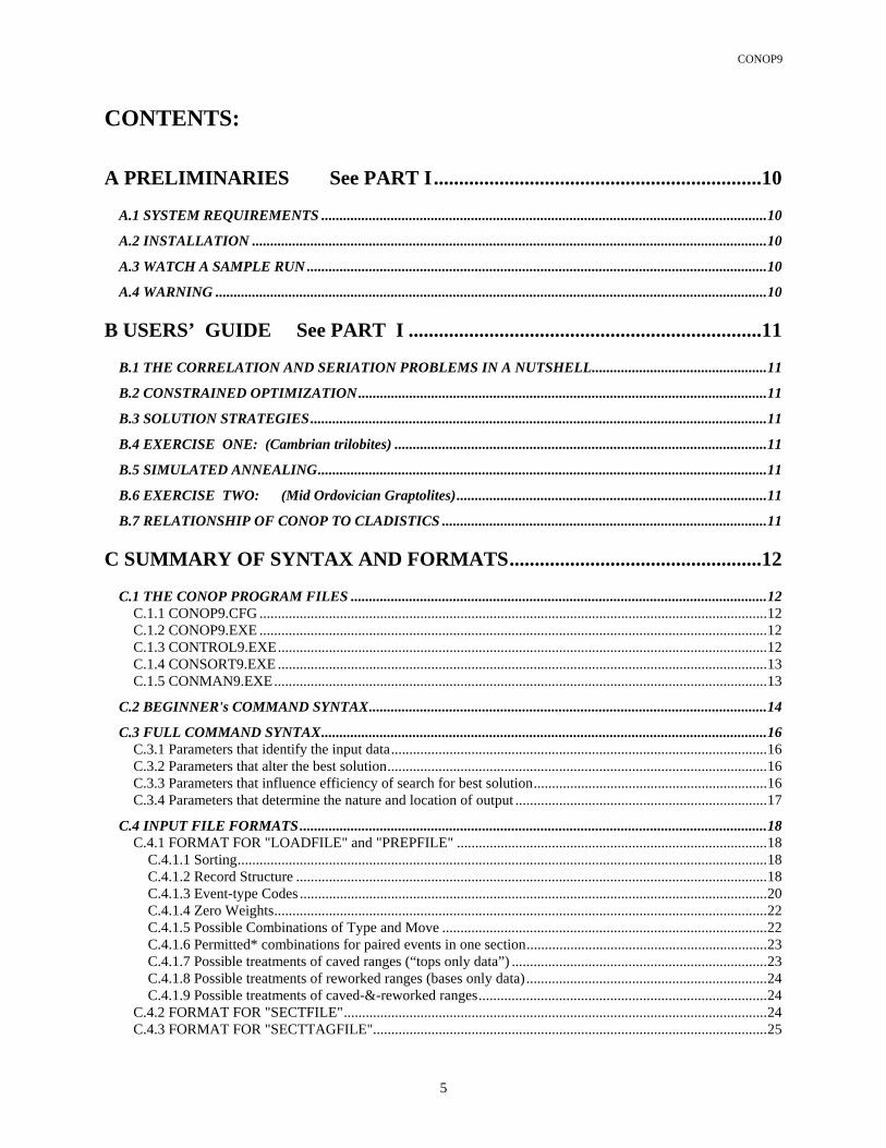
CONOP9

5

CONTENTS:

A PRELIMINARIES See PART I.................................................................10

A.1 SYSTEM REQUIREMENTS ..........................................................................................................................10 A.2 INSTALLATION .............................................................................................................................................10 A.3 WATCH A SAMPLE RUN ..............................................................................................................................10 A.4 WARNING .......................................................................................................................................................10

B USERS’ GUIDE See PART I ......................................................................11

B.1 THE CORRELATION AND SERIATION PROBLEMS IN A NUTSHELL................................................11 B.2 CONSTRAINED OPTIMIZATION................................................................................................................11 B.3 SOLUTION STRATEGIES.............................................................................................................................11 B.4 EXERCISE ONE: (Cambrian trilobites) ......................................................................................................11 B.5 SIMULATED ANNEALING...........................................................................................................................11 B.6 EXERCISE TWO: (Mid Ordovician Graptolites).....................................................................................11 B.7 RELATIONSHIP OF CONOP TO CLADISTICS .........................................................................................11

C SUMMARY OF SYNTAX AND FORMATS..................................................12

C.1 THE CONOP PROGRAM FILES ..................................................................................................................12 C.1.1 CONOP9.CFG ...........................................................................................................................................12 C.1.2 CONOP9.EXE ...........................................................................................................................................12 C.1.3 CONTROL9.EXE......................................................................................................................................12 C.1.4 CONSORT9.EXE ......................................................................................................................................13 C.1.5 CONMAN9.EXE.......................................................................................................................................13

C.2 BEGINNER's COMMAND SYNTAX.............................................................................................................14 C.3 FULL COMMAND SYNTAX..........................................................................................................................16

C.3.1 Parameters that identify the input data.......................................................................................................16 C.3.2 Parameters that alter the best solution........................................................................................................16 C.3.3 Parameters that influence efficiency of search for best solution................................................................16 C.3.4 Parameters that determine the nature and location of output .....................................................................17

C.4 INPUT FILE FORMATS................................................................................................................................18 C.4.1 FORMAT FOR "LOADFILE" and "PREPFILE" .....................................................................................18

C.4.1.1 Sorting.................................................................................................................................................18 C.4.1.2 Record Structure .................................................................................................................................18 C.4.1.3 Event-type Codes ................................................................................................................................20 C.4.1.4 Zero Weights.......................................................................................................................................22 C.4.1.5 Possible Combinations of Type and Move .........................................................................................22 C.4.1.6 Permitted* combinations for paired events in one section..................................................................23 C.4.1.7 Possible treatments of caved ranges (“tops only data”) ......................................................................23 C.4.1.8 Possible treatments of reworked ranges (bases only data)..................................................................24 C.4.1.9 Possible treatments of caved-&-reworked ranges...............................................................................24

C.4.2 FORMAT FOR "SECTFILE"....................................................................................................................24 C.4.3 FORMAT FOR "SECTTAGFILE"............................................................................................................25

CONOP9

6

C.4.4 FORMAT FOR "SECTTAGS"..................................................................................................................25 C.4.5 FORMAT FOR "LABELFILE".................................................................................................................25 C.4.6 FORMAT FOR "EVENTFILE" ................................................................................................................26 C.4.7 FORMAT FOR "EVENTTAGFILE" ........................................................................................................27 C.4.8 FORMAT FOR "EVENTTAGS" ..............................................................................................................28

C.5 COMMAND REFERENCE ...........................................................................................................................29 C.5.1 PARAMETERS THAT IDENTIFY THE INPUT DATA ( &getinn /).....................................................29

C.5.1.1 PROJECT............................................................................................................................................29 C.5.1.2 SECTIONS .........................................................................................................................................29 C.5.1.3 TAXA .................................................................................................................................................29 C.5.1.4 EVENTS .............................................................................................................................................29 C.5.1.5 MAX_LEVEL.....................................................................................................................................30 C.5.1.6 MAX_LABEL ....................................................................................................................................30 C.5.1.7 LOADFILE.........................................................................................................................................30 C.5.1.8 PREPFILE ..........................................................................................................................................30 C.5.1.9 SECTFILE ..........................................................................................................................................31 C.5.1.10 SECTTAGFILE ................................................................................................................................31 C.5.1.11 SECTTAGS ......................................................................................................................................32 C.5.1.12 LABELFILE .....................................................................................................................................32 C.5.1.13 EVENTFILE.....................................................................................................................................32 C.5.1.14 EVENTTAGFILE.............................................................................................................................32 C.5.1.15 EVENTTAGS...................................................................................................................................33 C.5.1.16 BESTKNOWN .................................................................................................................................33

C.5.2 PARAMETERS THAT ALTER THE BEST SOLUTION ( &getans /) ...................................................33 C.5.2.1 PENALTY ..........................................................................................................................................34 C.5.2.2 WEIGHTING......................................................................................................................................39 C.5.2.3 EXCLUSIVES ....................................................................................................................................40 C.5.2.4 FORCEFb4L.......................................................................................................................................40 C.5.2.5 FORCECOEX.....................................................................................................................................41 C.5.2.6 LETCONTRACT................................................................................................................................42 C.5.2.7 HOMERANGE...................................................................................................................................43 C.5.2.8 NEARENOUGH.................................................................................................................................44 C.5.2.9 USENEGATIVE.................................................................................................................................44 C.5.2.10 SMOOTHER.....................................................................................................................................46 C.5.2.11 SQUEEZER ......................................................................................................................................46 C.5.2.12 SHRINKER ......................................................................................................................................46 C.5.2.13 TEASER ...........................................................................................................................................47 C.5.2.14 STACKER ........................................................................................................................................47

C.5.3 PARAMETERS THAT INFLUENCE EFFICIENCY OF SEARCH FOR BEST SOLUTION ...............48 C.5.3.1 SOLVER.............................................................................................................................................49 C.5.3.2 STEPS.................................................................................................................................................51 C.5.3.3 TRIALS ..............................................................................................................................................52 C.5.3.4 STARTEMP........................................................................................................................................53 C.5.3.5 RATIO ................................................................................................................................................53 C.5.3.6 HOODSIZE ........................................................................................................................................54 C.5.3.7 STARTYPE ........................................................................................................................................56 C.5.3.8 STARTSECT ......................................................................................................................................57 C.5.3.9 STARTEVENT...................................................................................................................................57 C.5.3.10 SHOWMOVIES ...............................................................................................................................58 C.5.3.11 TRAJECTORY.................................................................................................................................60 C.5.3.12 VIDEOMODE ..................................................................................................................................60 C.5.3.13 PAUSES............................................................................................................................................61 C.5.3.14 CURVFILE.......................................................................................................................................63 C.5.3.15 CRV2FILE........................................................................................................................................64

CONOP9

7

C.5.4 PARAMETERS THAT DETERMINE NATURE AND LOCATION OF OUTPUT DATA ..................64 C.5.4.1 COLUMNS.........................................................................................................................................64 C.5.4.2 UNLOADMAIN.................................................................................................................................64 C.5.4.3 UNLOADSECT..................................................................................................................................65 C.5.4.4 UNLOADEVNT.................................................................................................................................66 C.5.4.5 [REPORT -] ........................................................................................................................................66 C.5.4.6 [CUSTOM -].......................................................................................................................................66 C.5.4.7 STARTFILE .......................................................................................................................................66 C.5.4.8 STEPFILE...........................................................................................................................................67 C.5.4.9 BESTARTFILE ..................................................................................................................................67 C.5.4.10 CULLFILE........................................................................................................................................68 C.5.4.11 OBSDFILE .......................................................................................................................................68 C.5.4.12 PLCDFILE........................................................................................................................................68 C.5.4.13 EXTNFILE .......................................................................................................................................69 C.5.4.14 COMPOSFILE..................................................................................................................................69 C.5.4.15 COMPOSNMBR ..............................................................................................................................69 C.5.4.16 COMPOSTYPE ................................................................................................................................69 C.5.4.17 SOLNLIST........................................................................................................................................73 C.5.4.18 COEXISTFILE .................................................................................................................................73 C.5.4.19 FAD_LADFILE................................................................................................................................74 C.5.4.20 CURVFILE.......................................................................................................................................74 C.5.4.21 CRV2FILE........................................................................................................................................74 C.5.4.22 RUNLOGFILE .................................................................................................................................74

C.6 CONOP9 “SCREEN LIST OUTPUT” MENU ...........................................................................................76 C.6.1 LIST BEST SEQUENCE ..........................................................................................................................78 C.6.2 BEST SEQUENCE....................................................................................................................................78 C.6.3 Log Out CONOP9 .....................................................................................................................................78

C.7 CONOP9 “GRAPHICAL OUTPUT” MENU.............................................................................................80 C.7.1 RELAXED-FIT CURVES.........................................................................................................................82 C.7.2 BEST-FIT INTERVALS ...........................................................................................................................84 C.7.3 EVENT CULLING CIRCLES...................................................................................................................84 C.7.4 TAXON DURATIONS .............................................................................................................................86 C.7.5 RANGE EXTENSIONS ............................................................................................................................86 C.7.6 TAXON DIVERSITY ...............................................................................................................................86 C.7.7 MEAN EXTANT TAXON LONGEVITY................................................................................................87 C.7.8 PACE of ORIGINATION/EXTINCTION ................................................................................................88 C.7.9 PAIRWISE CONTRADICTIONS.............................................................................................................88 C.7.10 The TAXON RANGE CHARTS.............................................................................................................91 C.7.11 COMPOSITE RANGE INCREMENTS..................................................................................................92 C.7.12 COLLECTION QUALITY......................................................................................................................98 C.7.13 2-SECTION LOCs...................................................................................................................................98 C.7.14 FENCE CHARTS ..................................................................................................................................101 C.7.15 SECTION RANGE CHARTS ...............................................................................................................101 C.7.16 RERUN SEARCH; NO OUTOUT FILE...............................................................................................106 C.7.17 Log Out CONOP9 .................................................................................................................................106

C.8 CONOP9 “TEXT-FILE OUTPUT” MENU .............................................................................................107 C.8.1 SECTION PENALTIES .........................................................................................................................107 C.8.2 EVENT PENALTIES ..............................................................................................................................108 C.8.3 RANGE CHARTS...................................................................................................................................109 C.8.4 RANGE SEQUENCE..............................................................................................................................109 C.8.5 COMPOSITE RANGES..........................................................................................................................110 C.8.6 TAXON RANGES ..................................................................................................................................111 C.8.7 Smoothed Line of Correlation..................................................................................................................112

CONOP9

8

C.8.8 Log Out CONOP9 ...................................................................................................................................113 C.9 CONTROL9 MENU OPTIONS ...................................................................................................................114

C.9.1 STANDARD REPORTS .........................................................................................................................114 C.9.1.1 Section Listing ..................................................................................................................................114 C.9.1.2 Event Listing.....................................................................................................................................116 C.9.1.3 Coexistence Listing...........................................................................................................................117 C.9.1.4 Coexistence Counting .......................................................................................................................118 C.9.1.5 Event Pairs ........................................................................................................................................118

C.9.2 STANDARD GRAPHICS.......................................................................................................................119 C.9.2.1 1-Section Range Charts.....................................................................................................................119 C.9.2.2 2-Section Range Coordinates............................................................................................................119 C.9.2.3 Crossover Fence Diagram.................................................................................................................119

C.9.3 ADVANCED GRAPHICS ......................................................................................................................119 C.9.3.1 Shared Events ...................................................................................................................................120 C.9.3.2 Pairwise Sequence Mis-Matches ......................................................................................................120 C.9.3.3 Taxon Coexistence Matrix ................................................................................................................120 C.9.3.4 Event Order Matrix ...........................................................................................................................120 C.9.3.5 Instance Size Statistics ......................................................................................................................120 C.9.3.6 Distance Between Events..................................................................................................................120

C.9.4 EXPERIMENTAL GRAPHICS ..............................................................................................................121 C.9.4.1 Point Search on Penalty Landscape ..................................................................................................121 C.9.4.2 Chain Search on Penalty Changes ....................................................................................................121 C.9.4.3 Star Search on Penalty Changes........................................................................................................121 C.9.4.4 Droplet Search on Penalty Changes..................................................................................................122 C.9.4.5 Bubble Search on Penalty Changes ..................................................................................................122 C.9.4.6 Local Minimum Penalties .................................................................................................................122

C.9.5 Log Off CONTROL9...............................................................................................................................122 C.10 TROUBLE SHOOTING..............................................................................................................................123

C.10.1 PATH ERRORS.....................................................................................................................................123 C.10.2 FILE EXTENSIONS .............................................................................................................................123 C.10.3 KEYWORD ERRORS...........................................................................................................................123 C.10.4 CURVFILE ERRORS ...........................................................................................................................123 C.10.5 INPUT FILE ERRORS..........................................................................................................................124 C.10.6 CONFIGURATION FILE ERRORS.....................................................................................................124 C.10.7 EXIT ANOMALIES..............................................................................................................................124 C.10.8 VIEW ANOMALIES ............................................................................................................................124 C.10.9 QUIKWIN MEMORY ANOMALIES ..................................................................................................124 C.10.10 GRAPHICAL OUTPUT ANOMALIES .............................................................................................125 C.10.11 CONSORT ANOMALIES ..................................................................................................................125 C.10.12 CONTROL ANOMALIES ..................................................................................................................125

D APPENDICES ................................................................................................. 126

D.1 REFERENCES (See Part I)........................................................................................................................126 D.2 The CONOP Program Family HISTORY ....................................................................................................126

D.2.1 CONOP.EXE and CONOP2.EXE...........................................................................................................126 D.2.2 CONOP3.EXE.........................................................................................................................................126 D.2.3 CONOP9.EXE.........................................................................................................................................126 D.2.4 CONOP9 compared with CONOP3 ........................................................................................................130 D.2.5 DEC versions compared with MS versions .............................................................................................130 D.2.6 CONSORT9.EXE and CONTROL9.EXE...............................................................................................130 D.2.7 CONMAN9.EXE.....................................................................................................................................131

CONOP9

9

___________________________ .........................................................................................................................131 CONMAN VERSION HISTORY.........................................................................................................................131 _____________________________________________________ .....................................................................134 MAXIMUM SIZE LIMITATIONS FOR CONMAN DATA SETS ....................................................................134

D.2.8 RILE7x62.DAT .......................................................................................................................................135 D.2.9 RILEY7.SCT ...........................................................................................................................................137 D.2.10 RILEY62.EVT.......................................................................................................................................137 D.2.11 BEST KNOWN PENALTIES and COOLING SCHEDULES .............................................................137 D.2.12 An Abbreviated* Sample Output Text File ...........................................................................................138

D.3 SAMPLE DATA Ordovician Mohawk Valley.............................................................................................142 D.3.1 MO6x21x7.DAT......................................................................................................................................142 D.3.2 MOHAWK6.SCT ....................................................................................................................................143 D.3.3 MOHAWK28.EVT..................................................................................................................................143

D.4 THE CONFIGURATION FILE: CONOP9.CFG .......................................................................................144

E INDEX .............................................................................................................. 149

CONOP9 PART C REFERENCE

10

A PRELIMINARIES See PART I Starting with version 6.4 the Users’ Guide and Reference Manual were split into two documents. Look for Part I in Guide.doc or Guide.pdf. With the prototype of CONMAN.EXE a third volme “Getting Started” was begun in 2005. It deals with the preparation of input files for CONOP9. The following subsections of instructions will be found in the User’s Guide: A.1 SYSTEM REQUIREMENTS

A.2 INSTALLATION

A.3 WATCH A SAMPLE RUN

A.4 WARNING

CONOP9 PART C REFERENCE

11

B USERS’ GUIDE See PART I Starting with version 6.4 the Users’ Guide and Reference Manual were split into two documents. Look for Part I in Guide.doc or Guide.pdf. The following subsections will be found there: B.1 THE CORRELATION AND SERIATION PROBLEMS IN A NUTSHELL

B.2 CONSTRAINED OPTIMIZATION

B.3 SOLUTION STRATEGIES

B.4 EXERCISE ONE: (CAMBRIAN TRILOBITES)

B.5 SIMULATED ANNEALING

B.6 EXERCISE TWO: (MID ORDOVICIAN GRAPTOLITES)

B.7 RELATIONSHIP OF CONOP TO CLADISTICS

CONOP9 PART C REFERENCE

12

C SUMMARY OF SYNTAX AND FORMATS C.1 THE CONOP PROGRAM FILES C.1.1 CONOP9.CFG The CONFIGURATION FILE: CONOP9.CFG is a text-file of user-editable run-time parameters for CONOP9.EXE. CONOP9.EXE solves a stratigraphic correlation problem based on the data in LOADFILE and writes answers to UNLOADMAIN, with or without UNLOADSECT, UNLOADEVNT and RUNLOGFILE, as instructed by CONOP9.CFG. CONOP9.CFG is also used by CONSORT9.EXE, which takes the preliminary PREPFILE listing and expands it by assigning the sequential numbers to collecting LEVELS, expanding top-only and bottom-only taxon entries, sorting the sequence of records, and writing the LOADFILE for CONOP9 to use. CONOP9.CFG is also used by CONTROL9.EXE, which examines all aspects of the LOADFILE data that do not require finding the best solution. LOAD THIS FILE (CONOP9.CFG) TO SAME DIRECTORY AS CONOP9.EXE, CONSORT9.EXE and CONTROL9.EXE. The name of this configuration file and the assumption that it resides with the EXE files is hard-coded into the EXE files. This condition cannot be altered except at source code level. Edit this file using any word processor that can save it as an ASCII text-file without formatting. Microsoft Word and WordPad are suitable. WordPad loads and unloads faster. Windows Notepad cannot edit the file unless it is shortened. Editing instructions are attached to the shipped version of the file. These instructions are reproduced in this guide and reference manual; so they may be deleted from CONOP9.CFG to shorten it considerably. C.1.2 CONOP9.EXE [CURRENT] The MAIN EXECUTABLE FILE: CONOP9.EXE solves a stratigraphic correlation problem as instructed by parameter settings in CONOP9.CFG. It reads the raw stratigraphic data from the file identified by the LOADFILE parameter and any accompanying event and section dictionaries. It reports its solution and analysis to the file named in the UNLOADMAIN parameter, with or without additional reports as directed by the UNLOADSECT, UNLOADEVNT and RUNLOGFILE parameters in CONOP9.CFG. These are annotated text files suitable for word processing. CONOP9.EXE also writes a series of unannotated data files suitable for spreadsheet programs or other programs designed for numerical analysis. Some of these data files may be read by CONOP9.EXE to initialize subsequent runs. Others may be updated as a summary of multiple runs. LOAD THIS FILE (CONOP9.EXE) TO SAME DIRECTORY AS CONOP9.CFG. C.1.3 CONTROL9.EXE [OBSOLETE] An AUXILLIARY EXECUTABLE FILE: CONTROL9.EXE examines (“trolls”) all aspects of the LOADFILE data that do not require finding the best solution. CONTROL9 has a run-time, drop down menu of options to analyze the input data set or map the penalty landscape. The CONTROL9 options fall into three categories: "standard," "advanced," and "experimental." Sadler uses the "experimental" options to map the problem landscape; they have very long run-times and are not at all user-friendly. Development and support of this file ceased with the development of CONMAN9, although that program does not replace all the functions of CONTROL9. CONTROL9 is no longer developed and supported. Many of its

CONOP9 PART C REFERENCE

13

functions are not feasible for the large data sets compiled since 2001, either because the run-times are too long or the summary graphics are illegible for such large data volumes. LOAD THIS FILE (CONTROL9.EXE) TO SAME DIRECTORY AS CONOP9.CFG. C.1.4 CONSORT9.EXE [OBSOLETE] A second AUXILLIARY EXECUTABLE FILE: CONSORT9.EXE takes the preliminary PREPFILE listing and expands it by assigning the sequential numbers to collecting LEVELS, expanding top-only and bottom-only taxon entries, sorting the sequence of records, and writing the LOADFILE for CONOP9 to use. CONSORT9 also provides options to edit the weighting factors in LOADFILE. i.e. all input preparation. CONSORT9.EXE allows the stratigrapher to prepare a data file that does not meet all the rigors of the LOADFILE required by CONOP9.EXE. It is a preprocessor. Two particularly irksome requirements are dropped: the file identified by the PREPFILE parameter need not be sorted; and it is not necessary to assign sequential integers to the collecting horizons in each section. In the unsorted file, new records may be added to the end in any order. The addition of new finds from existing sections typically causes the horizon numbering to change – a very disagreeable editing chore. CONSORT9.EXE does not yet relax the requirement to give sections and taxa sequential integer codes with no gaps. Thus, sections and taxa cannot be so simply removed from the input files. The alternative is to weight them zero. CONSORT9.EXE provides the ability to change the weights for all records that pertain to a particular event, event type, taxon, or section. This file has been obsolete since the development of CONMAN9 and is not longer supported. LOAD THIS FILE (CONSORT9.EXE) TO SAME DIRECTORY AS CONOP9.CFG. C.1.5 CONMAN9.EXE [CURRENT] This executable file is a custom data manager for CONOP9 with graphical user interfaces. It replaces CONSORT9 and several features of CONTROL9 and was first beta-tested in 2004. It maintains several files; those marked with an asterisk are optional:

a section dictionary a taxon dictionary a synonym dictionary* a multinym dictionary* an event dictionary a bibliographic reference dictionary one range-chart file for each section

The program offers several menus: Analysis List/Edit - options to list and edit data files Proof - options to scan data files for known errors and warnings Append - options to add new taxa, events, references, sections, ranges etc Synonyms - options to manage synonyms Export - writes input files for CONOP9

CONOP9 PART C REFERENCE

14

C.2 BEGINNER'S COMMAND SYNTAX The following providesnon-technical instructions for a safe minimalist approach to editing CONOP9.CFG. All the commands are listed as in the configuration file, so that you can find them. Only the bold lines really need attention. Italics indicate safe items that you might as well edit for convenience. Annotations in parentheses suggest whether and when the other lines might be considered. Many of the parameters were designed for special needs and peculiar experiments; they should be ignored as advised below. The reference manual explains their use and often recommends against their use. Note these generalizations:

0. It is assumed that the problem is a correlation, not a seriation 1. It is assumed that the instance contains less than 20 sections and less than 100 taxa

If the instance is larger, increase the number of TRIALS. 2. Lines in bold face require planning; they must match your instance of the problem. 3. Items in italics are text strings that should be replaced with more meaningful entries. 4. Other command settings may be copied as is (without the trailing comments!). 5. File extension convention is not mandatory.

Files with .txt extension are annotated for reading in users’ word processor. Files with .dat extension are designed for loading FORTRAN arrays; explore with spreadsheet.

If the data have been compiled in CONMAN9, the export menu offers options to automate the construction of the CONOP.CFG with different degrees of user editing. Start by letting CONMAN9 write a CONOP9.CFG file; open and examine it as a first step in learning to set the parameters STEPS, TRIALS, STARTEMP, and RATIO according to the size of the data set. ___________________ PROJECT= 'any old title will do' SECTIONS= number of sections in your input data (MUST BE CORRECT) TAXA= number of taxa in your input data (MUST BE CORRECT) EVENTS= number of other correlation events in your input dat (MUST BE CORRECT) MAX_LEVELS= 150 (need only be bigger than needed) MAX_LABELS= 15 (need only be bigger than needed) LOADFILE= ‘your path\your input data file name.dat’ (MUST BE CORRECT; default path is folder with

CONOP9.EXE) PREPFILE= ‘same as input file’ (no consequence for CONOP9.EXE) SECTFILE= ‘OFF’ (your section dictionary if available) SECTTAGFILE= ‘OFF’ (optional coding of sections; e.g. latitude zones) SECTTAGS= ‘OFF’ (section code dictionary, if needed) LABELFILE= ‘OFF’ (your label dictionary; forget about it!) EVENTFILE= ‘OFF’ (your event dictionary if available) EVENTTAGFILE= ‘OFF’ (optional coding of events; e.g. families) EVENTTAGS = ‘OFF’ (event code dictionary, if needed) BESTKNOWN 0.0 (no consequence) ________________________ PENALTY= 'LEVEL' (an acceptable option for nearly all data sets) LETCONTRACT= 'OFF' (don't even think about it!) WEIGHTING= 'ON' (don't even think about it unless doing seriation!) USENEGATIVE= 'OFF' (all the other options are unsafe at any speed) NEARENOUGH= 0.0 (mostly harmless) EXCLUSIVES= 'no’ (don't even think about it!) FORCECOEX= 'SL’ ('SS' would not hurt) FORCEFb4L= 'OFF’ ('ON' would not hurt unless the instance is very large and memory limited) HOMERANGE= 'SL' ('SS' would not hurt)

CONOP9 PART C REFERENCE

15

SMOOTHER= 0.0 (don't even think about it unless mimicking Shaw’s method) SQUEEZER= 0.0 (don't even think about it!) SHRINKER= 0.0 (don't even think about it!) TEASER= 0.0 (don't even think about it unless doing seriation!) STACKER= 'OFF' (don't even think about it unless doing seriation!) __________________________ SOLVER 'ANNEAL' (an almost universally appropriate option) STEPS= 500 (may need adjustment for more efficient solution) TRIALS= 200 (may need adjustment for more efficient solution) STARTEMP= 100 (may need adjustment for more efficient solution) RATIO= 0.98 (may need adjustment for more efficient solution) HOODSIZE= 'BIG’ (an almost universally appropriate option) STARTYPE= 'RAND' (change to 'FILE' to continue last run) STARTSECT= 1 (ignore!) STARTEVENT= 1 (ignore!) SHOWMOVIES= 'CHT' (ignore!) TRAJECTORY= 'ALL' (ignore!) VIDEOMODE= 'SVGA' (ignore!) PAUSES= 'ON' (ignore for now) CURVFILE= 'OFFcurve.dat' (ignore for now) CRV2FILE= 'OFFcurve2.dat' (ignore for now) ________________ COLUMNS= 7 UNLOADMAIN= 'outmain.txt' (without path, CONOP writes to its own folder) FITS_OUT= 'ON' (get a full analysis of the solution) CNFG_OUT= 'ON' (get a full analysis of the solution) SEQN_OUT= 'ON' (get a full analysis of the solution) INCR_OUT= 'ON' (get a full analysis of the solution) LOC_OUT= 'ON' (get a full analysis of the solution) OBS_OUT= 'ON' (get a full analysis of the solution) COMP_OUT= 'ON' (get a full analysis of the solution) UNLOADSECT= 'outsect.txt' (without path, CONOP writes to its own folder) SECT_OUT= 'OFF' (otherwise, this may write a very big file) UNLOADEVNT= 'outevnt.txt' (without path, CONOP writes to its own folder) EVNT_OUT= 'OFF' (otherwise, this may write a very big file) COEX_OUT= 'OFF' (otherwise, this may write a very big file) CULLFILE= 'cull.dat (rarely needed) RUNLOGFILE= 'runlog.txt' (without path, CONOP writes to its own folder) SOLNLIST= 'OFF' (rarely needed) STARTFILE= 'soln.dat' (needed to continue the previous run) STEPFILE= 'OFF' (rarely needed) BESTARTFILE= 'bestsoln.dat' (might not be written) COMPOSFILE= 'cmpst.dat' (easier to read in outmain.txt) COMPOSNMBR= 0 (ignore) COMPOSTYPE= 'ZST' (other settings generally inferior) OBSDFILE= 'obsd.dat' (easier to read in outmain.txt) PLCDFILE= 'plcd.dat' (easier to read in outmain.txt) EXTNFILE= 'extn.dat' (easier to read in outmain.txt) COEXISTFILE= 'coex.dat' (only useful if restarting a very big data set) FAD_LADFILE= 'Fb4L.dat' (only useful if restarting a very big data set) ORDERFILE= 'order.dat' (not needed)

CONOP9 PART C REFERENCE

16

C.3 FULL COMMAND SYNTAX Notes

1. The order and grouping of commands matches CONOP9.CFG 2. Inverted commas are required to delimit text strings as shown 3. The vertical bar ( | ) separates different items in option lists 4. Bold face indicates the safe/standard options 5. Bold-italic face indicates other frequently used options. 6. Square brackets indicate items that must be replaced by appropriate numbers or strings. 7. Conventional file names and/or extensions are suggested where appropriate.

Note also: by preparaing input files through CONMAN9, it is possible to automate all of the preparation of the CONOP9.CFG file. Parameter keywords are chosen to fit the selected number of sections, taxa, and other events. C.3.1 PARAMETERS THAT IDENTIFY THE INPUT DATA

( &getinn / PARAMETER LIST)

PROJECT= ['project name for use in titles'] SECTIONS= [integer] TAXA= [integer] EVENTS= [integer] MAX_LEVELS= [integer] MAX_LABELS= [integer] LOADFILE= ['path\filename.dat'] PREPFILE= ['path\filename.dis'] SECTFILE= ['path\filename.sct' | 'OFFpath\filename.sct' | 'OFF']

SECTTAGFILE= ['path\filename.sct' | 'OFFpath\filename.sct' | 'OFF'] SECTTAGS= ['path\filename.sct' | 'OFFpath\filename.sct' | 'OFF'] LABELFILE= ['path\filename.evt' | 'OFFpath\filename.evt' | 'OFF']

EVENTFILE= ['path\filename.evt' | 'OFFpath\filename.evt' | 'OFF'] EVENTTAGFILE= ['path\filename.sct' | 'OFFpath\filename.sct' | 'OFF'] EVENTTAGS= ['path\filename.sct' | 'OFFpath\filename.sct' | 'OFF']

BESTKNOWN= [0 or real number > 0.0] C.3.2 PARAMETERS THAT ALTER THE BEST SOLUTION

( &getans / Parameter LIST)

PENALTY= 'INTERVAL' | 'LEVEL' |’EVENTUAL’| 'ORDINAL' | 'SPATIAL' | 'RASCAL' | ‘ROYAL’ | ’SEQUEL’ LETCONTRACT= 'FILE' | 'OFF' | 'SS' | 'SL' WEIGHTING = 'FILE' | 'OFF' | 'ON' | 'COEX%1' | 'COEX%2' | 'COEX%5' | 'COEX%10' | 'COEX%15'

| 'COEX%20' | 'COEX^-1' | 'COEX^-2' | 'COEX^-3' | 'COEX' | 'COEX2' | 'COEX3' USENEGATIVE= 'ON' | 'OFF' | 'COEX' | 'SS' | 'SL' NEARENOUGH= [0.0 or real number >0.0] EXCLUSIVES= 'NO' | 'YES' FORCECOEX= 'SS' | 'SL' | 'OFF' | 'FILE' FORCEFb4L= ‘ON’|’OFF’ HOMERANGE= 'SS' | 'SL' SMOOTHER= [0.0 or real number >0.0] SQUEEZER= [0.0 or real number >0.0] SHRINKER= [0.0 or real number >0.0] TEASER= [0.0 or real number >0.0] STACKER= 'OFF' | 'THRU' | 'INCL' | 'FREQ' | 'DIST' | 'EXIT' | 'PROP' | ‘SPAN’ | 'OLAP' | ‘COEX’

C.3.3 PARAMETERS THAT INFLUENCE EFFICIENCY OF SEARCH FOR BEST

SOLUTION ( &getrun / PARAMETER LIST)

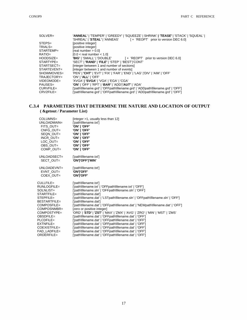
CONOP9 PART C REFERENCE

17

SOLVER= 'ANNEAL' | 'TEMPER' | 'GREEDY' | 'SQUEEZE' | SHRINK' | 'TEASE' | 'STACK' | 'SQUEAL' |

'SHREAL' | 'STEAL' | 'ANNEAS' [ + 'REOPT' prior to version DEC 6.0] STEPS= [positive integer] TRIALS= [positive integer] STARTEMP= [real number > 0.0] RATIO= [0.0 < real number < 1.0] HOODSIZE= 'BIG' | 'SMALL' | 'DOUBLE' [ + 'REOPT' prior to version DEC 6.0] STARTYPE= 'SECT' | 'RAND' | 'FILE' | ‘STEP’ | ‘BEST’|’CONT’ STARTSECT= [integer between 1 and number of sections] STARTEVENT= [integer between 1 and number of events] SHOWMOVIES= 'PEN' | 'CHT' | 'EVT' | 'FIX' | 'FAR' | ‘END’ | 'LAG' |’DIV’ | 'AIM' | 'OFF' TRAJECTORY= 'ON' | 'ALL' | 'OFF' VIDEOMODE= 'XVGA' | 'SVGA' | 'VGA' | 'EGA' | 'CGA' PAUSES= 'ON' | 'OFF' | 'RPT' | ‘BAR’ | 'ADD'|’AUT’ | ‘ADA’ CURVFILE= ['path\filename.grd' | 'OFFpath\filename.grd' | 'ADDpath\filename.grd' | 'OFF'] CRV2FILE= ['path\filename.grd' | 'OFFpath\filename.grd' | 'ADDpath\filename.grd' | 'OFF']

C.3.4 PARAMETERS THAT DETERMINE THE NATURE AND LOCATION OF OUTPUT

( &getout / Parameter List)

COLUMNS= [integer >1, usually less than 12] UNLOADMAIN= ['path\filename.txt'] FITS_OUT= 'ON' | 'OFF' CNFG_OUT= 'ON' | 'OFF' SEQN_OUT= 'ON' | 'OFF' INCR_OUT= 'ON' | 'OFF' LOC_OUT= 'ON' | 'OFF' OBS_OUT= 'ON' | 'OFF' COMP_OUT= 'ON' | 'OFF' UNLOADSECT= ['path\filename.txt'] SECT_OUT= 'ON'|'OFF'|’MIN’ UNLOADEVNT= ['path\filename.txt'] EVNT_OUT= 'ON'|'OFF' COEX_OUT= 'ON'|'OFF'

CULLFILE= ['path\filename.txt'] RUNLOGFILE= ['path\filename.txt' | 'OFFpath\filename.txt' | 'OFF'] SOLNLIST= ['path\filename.sln' | 'OFFpath\filename.sln' | 'OFF'] STARTFILE= ['path\filename.dat'] STEPFILE= ['path\filename.dat' | 'LSTpath\filename.sln' | 'OFFpath\filename.sln' | 'OFF'] BESTARTFILE= ['path\filename.dat'] COMPOSFILE= ['path\filename.dat' | 'OFFpath\filename.dat' | 'NEWpath\filename.dat' | ‘OFF'] COMPOSNMBR= [zero or positive integer] COMPOSTYPE= 'ORD' | 'STD' | 'ZST' | 'MAX' | 'ZMX' | 'AVG' | ‘ZRO’ | 'MIN' | ‘MST’ | ‘ZMS’ OBSDFILE= ['path\filename.dat' | 'OFFpath\filename.dat' | 'OFF'] PLCDFILE= ['path\filename.dat' | 'OFFpath\filename.dat' | 'OFF'] EXTNFILE= ['path\filename.dat' | 'OFFpath\filename.dat' | 'OFF'] COEXISTFILE= ['path\filename.dat' | 'OFFpath\filename.dat' | 'OFF'] FAD_LADFILE= ['path\filename.dat' | 'OFFpath\filename.dat' | 'OFF'] ORDERFILE= ['path\filename.dat' | 'OFFpath\filename.dat' | 'OFF']

CONOP9 PART C REFERENCE

18

C.4 INPUT FILE FORMATS NOTE: input files may be prepared automatically using the “Export” menu of the CONMAN9 program after all sections and taxa have been entered into this data manager. C.4.1 FORMAT FOR "LOADFILE" AND "PREPFILE" ASCII format; fields separated by blanks within records; records separated by a carriage return. Structure of fields and records is the same for LOADFILE and PREPFILE; but prepfile may be unsorted and levels need not be correct. C.4.1.1 SORTING “LOADFILE” MUST BE SORTED ON FIRST THREE FIELDS:

Primary Sort - field 1, event number, ascending Secondary Sort - field 2, event type, ascending Tertiary Sort - field 3, section number, ascending

"ascending" means first record (top of file) is event number 1 “PREPFILE” can be converted to LOADFILE format by running CONSORT9.EXE PREPFILE may eliminate the Level field or fill it with arbitrary integers. BUT, the sorting option in CONSORT9 must specify whether this field is present or not! C.4.1.2 RECORD STRUCTURE Each line in the file is considered a “record.” A record gives the level and weight for one event (e.g. FAD) as found in one section. Every record contains the same set of items, separated by blank spaces; each item is considered to be one “field” in the database record. The following field list is in the record order required for “PREPFILE” and “LOADFILE”: FIELD 1 Event Number

An integer that identifies the species or event These integers must be consecutive, starting with 1 (no gaps!)

FIELD 2 Event Type An integer code for the type of event

The following code numbers are defined for use or in development -3 unconstrained unpaired event [BOB] -2 unpaired disappearance event [DIS] -1 unpaired appearance event [APP] 0 spacer event (hiatus level) [GAP] under development 1 paired first appearance event [FAD] 2 paired last appearance event [LAD] 3 mid-range event [MID] 4 marker bed/event [ASH] 5 dated bed/event [AGE] 6 cycle boundary [CYC] under development

FIELD 3 Section Number

An integer corresponding to the section; sections must be numbered consecutively, starting with 1, and with no gaps!

FIELD 4 Horizon Position in stratigraphic distance from (arbitrary) base of section

CONOP9 PART C REFERENCE

19

An integer or decimal number (treated as decimal within the program) representing the stratigraphic position above the base of the section. Units of measurement are left to the user; because no unit conversion is made within the program, units are not needed. The base of the section SHOULD NOT be 0.00. It may be positive or negative. Internally, the program resets all section bases to 1000.00 and uses zeros to indicate missing events. Thus, field 4 values of 0.00 will likely be converted to non-zero values. But, for safety and compatibility with earlier versions of CONOP, 0.00 values should still be avoided. For well depths, values must have a negative sign; thus, the real values still increase up section for purposes of internal arithmetic. The top of the well may be 0.0 as long as the top is not an event horizon. The top of the well may have positive elevation; but it is best that no event level correspond to zero elevation.

FIELD 5 Level

An integer corresponding to the rank position of the event horizon in local section. Level numbers begin with 1 for the lowest event horizon and increase consecutively upward. A given level always has the same horizon value in one section. Because this number is easily assigned by the database manager or spreadsheet used to store the raw stratigraphic data, CONOP9.EXE does not attempt this task. However, the field may be left as zeros (or any integers) or even eliminated if the program CONSORT9.EXE is run before CONOP9.EXE. That sorting run will supply a menu choice between files that contain a level field and files that do not. Earlier versions used -1 for events known to extend below section and -2 for events known to extend above; This convention has been dropped. All range-end events recorded at the top or bottom levels of a section are assumed to be truncations and do not accrue a penalty. If a taxon is known to exist below the measured section, assign its FAD to the base (level 1). If the taxon is known to occur above the measured section assign its LAD to the section top. Observe this convention regardless of the apparent range ends within the section in order to achieve better results in seriation problems

FIELD 6 Moves Permitted

Integer code for freedom of placement. The following codes are defined: 0 = does not move (e.g. Type 4, 5 events; ASH, AGE) 1 = may move down section only (e.g. Type 1, -1 events: FAD, APP) 2 = may move up section only (e.g. Type 2, -2 events: LAD, DIS) 3 = may move up or down (e.g. Type 3, -3 events: MID, BOB) Types 4, 5, and 6, which were reserved but not used in earlier versions have been abandoned. Their anticipated purpose in treating reworked and caved events has been treated differently.

FIELD 7 Weight Up

Decimal-valued relative weight for up-section range extension; Default value is 1.00; may be larger or smaller than 1; larger values imply better established local range; may be set to zero for LAD to eliminate influence of event on solution, except through coexistence table. FOR DATED HORIZONS, this is the younger end of the range of probable age; i.e. SMALLER number. For dates in different sections, it is used for partial ordering. It may be set equal to Weight-Down to indicate that the age is certain. A full range of menu-driven editing options for resetting the weights is provided by CONSORT9.EXE.

FIELD 8 Weight Down

Decimal-valued relative weight for down-section range extension.

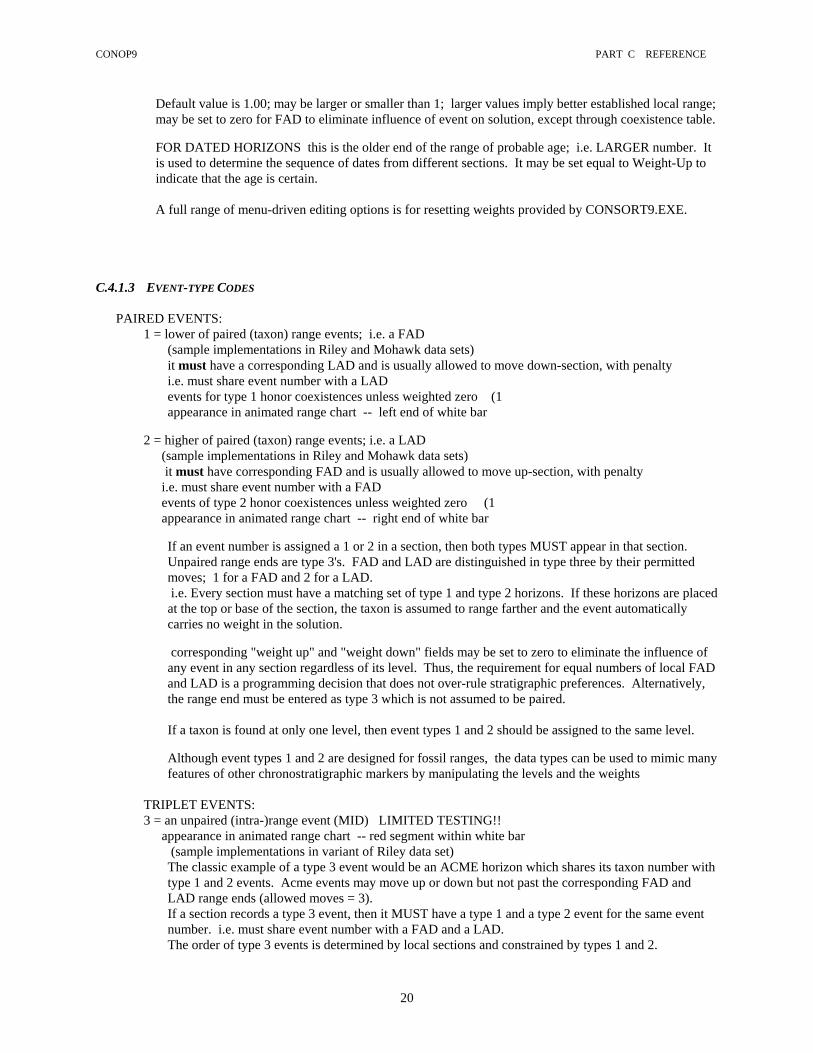
CONOP9 PART C REFERENCE

20

Default value is 1.00; may be larger or smaller than 1; larger values imply better established local range; may be set to zero for FAD to eliminate influence of event on solution, except through coexistence table. FOR DATED HORIZONS this is the older end of the range of probable age; i.e. LARGER number. It is used to determine the sequence of dates from different sections. It may be set equal to Weight-Up to indicate that the age is certain.

A full range of menu-driven editing options is for resetting weights provided by CONSORT9.EXE.

C.4.1.3 EVENT-TYPE CODES PAIRED EVENTS:

1 = lower of paired (taxon) range events; i.e. a FAD (sample implementations in Riley and Mohawk data sets) it must have a corresponding LAD and is usually allowed to move down-section, with penalty i.e. must share event number with a LAD events for type 1 honor coexistences unless weighted zero (1 appearance in animated range chart -- left end of white bar

2 = higher of paired (taxon) range events; i.e. a LAD

(sample implementations in Riley and Mohawk data sets) it must have corresponding FAD and is usually allowed to move up-section, with penalty i.e. must share event number with a FAD events of type 2 honor coexistences unless weighted zero (1 appearance in animated range chart -- right end of white bar

If an event number is assigned a 1 or 2 in a section, then both types MUST appear in that section. Unpaired range ends are type 3's. FAD and LAD are distinguished in type three by their permitted moves; 1 for a FAD and 2 for a LAD. i.e. Every section must have a matching set of type 1 and type 2 horizons. If these horizons are placed at the top or base of the section, the taxon is assumed to range farther and the event automatically carries no weight in the solution. corresponding "weight up" and "weight down" fields may be set to zero to eliminate the influence of any event in any section regardless of its level. Thus, the requirement for equal numbers of local FAD and LAD is a programming decision that does not over-rule stratigraphic preferences. Alternatively, the range end must be entered as type 3 which is not assumed to be paired. If a taxon is found at only one level, then event types 1 and 2 should be assigned to the same level. Although event types 1 and 2 are designed for fossil ranges, the data types can be used to mimic many features of other chronostratigraphic markers by manipulating the levels and the weights

TRIPLET EVENTS: 3 = an unpaired (intra-)range event (MID) LIMITED TESTING!!

appearance in animated range chart -- red segment within white bar (sample implementations in variant of Riley data set) The classic example of a type 3 event would be an ACME horizon which shares its taxon number with type 1 and 2 events. Acme events may move up or down but not past the corresponding FAD and LAD range ends (allowed moves = 3). If a section records a type 3 event, then it MUST have a type 1 and a type 2 event for the same event number. i.e. must share event number with a FAD and a LAD. The order of type 3 events is determined by local sections and constrained by types 1 and 2.

CONOP9 PART C REFERENCE

21

IN PREPFILE the type three has another purpose: it may be used to enter top-only or bottom-only events. The event might be a FAD (allowed moves = 1) without a corresponding LAD, or a LAD (allowed moves = 2) without the corresponding FAD. CONSORT9.EXE must be used to expand these types before running CONOP9EXE. The missing paired event is entered at the same level as the observed event, but weighted 0.1. Type 3 is altered to type 1 for FADs and type 2 for LADs.

UNPAIRED EVENTS: -1= an unpaired appearance event (APP); allowed to move down only

may be used for a FAD that lacks a reliable FAD designed for first appearance of character traits Type –1 events may not be mixed with FADs for same event number Type –1 events may not share event number with any other events

appearance in animated range chart -- yellow dash -2=an unpaired disappearance event (DIS); allowed to move up only

may be used for a LAD that lacks a reliable LAD designed for last appearance of character traits Type –2 events may not be mixed with LADs for same event number Type –2 events may not share event number with any other events

appearance in animated range chart -- yellow dash

-3=an unpaired unconstrained event; allowed to move up and down (BOB) may be used for any unconstrained event Type -3 events may not share event number with any other events

appearance in animated range chart -- yellow dash

4 = unique marker horizon (ASH); not allowed to move (sample implementations in Mohawk data set) Marker horizons may not be moved up- or down-section (allowed moves = 0). Their order is known only from the preservation sequence in local sections. They honor the order of superposition but do not play a role in coexistence. Type four events must be uniquely matched; i.e. every local observation of an event of type 4 with the same event number is assumed to be the same chronostratigraphic marker. The solution has no option but to correlate them. Type 4 events may not share event number with any other events

appearance in animated range chart -- yellow dash

5 = dated horizon (AGE); not allowed to move

(sample implementations in Mohawk data set) The order of dated horizons is known independently of local sections. The wtup and wtdown fields are used to record the range of possible age; e.g. plus and minus 2 sigma for a radiometric age determination. The dated horizons do not need to be found in more than one section to be useful; but there does need to be more than one dated horizon to influence the solution. Ordinarily, each dated horizon has a different event number. If the dated horizon is a marker bed known from more than one section, however, the same event number may be assigned in every section. Of course, the age range recorded in the weight fields should reflect the multiple age determinations.

Type 5 events do not move up or down section (allowed moves = 0), so the weight fields are not needed for their original purpose. Type 5 events may not share event number with any other events Type 5 events honors order of ages and superposition. They play no role in coexistence.

CONOP9 PART C REFERENCE

22

appearance in animated range chart -- yellow dash

6 = non-unique horizon (SEQ) NOT YET SUPPORTED; reserved for future development e.g. cycle or sequence boundary; undated polarity reversal Type 6 events will not move; they will be matched to any one of their kind. The weight fields will be used for parameters that determine the degree of match. appearance in animated range chart -- none

0 = hiatus (GAP) NOT YET SUPPORTED; reserved for future development

Hiatus horizons will not move. They will augment the penalty for range extensions and improve the translation from thickness to time.

appearance in animated range chart -- none C.4.1.4 ZERO WEIGHTS Both weight up and weight down may be set to zero for batches of locally observed events to eliminate the influence of a whole section or a whole taxon from the solution. This may be easier than re-numbering the taxa and/or sections to be consecutive from 1. Although the program has been made as robust as possible in the face of "zeroed out" sections and taxa, the stratigraphic consequences often require more careful analysis. Those taxa that are "zeroed out” of all sections may be placed almost anywhere in the final solution because their ranges can be extended without penalty! Events that are "zeroed out" are not used to fill out the coexistence matrix (a change from earlier versions of CONOP) and they have been eliminated from many of the graphical menu options. C.4.1.5 POSSIBLE COMBINATIONS OF TYPE AND MOVE TYPE - MOVE PURPOSE CODED? TESTED? NON-EVENTS (not in coexistence or partial ordering matrix)

0 - 0 spacers - add penalty for crossing No None PAIRED EVENTS/ENTRIES (in coexistence matrix):

1 - 1 reliable FAD with LAD(2,2) or LAD(2,3) Yes Many 1 - 3 caved FAD Part None 2 - 2 reliable LAD Yes Many 2 - 3 reworked LAD Part None

work-around forbidden combinations 1 - 0 perfect FAD! use very large weight 2 - 0 perfect LAD! use very large weight

"UNPAIRED" ENTRIES that will be converted to paired events (FAD and LAD together) by CONSORT9

3 - 2 unpaired reliable LAD Yes Some useful for coexistence matrix 3 - 1 unpaired reliable FAD Yes Some useful for coexistence matrix

UNPAIRED EVENTS/ENTRIES (in partial ordering matrix): taxon events:

-3 - 3 unconstrained BOB Part None -2 - 2 unpaired disappearance DIS Part Few -1 - 1 unpaired appearance APP Part Few 3 - 3 unpaired taxon event Yes Few without limit within range

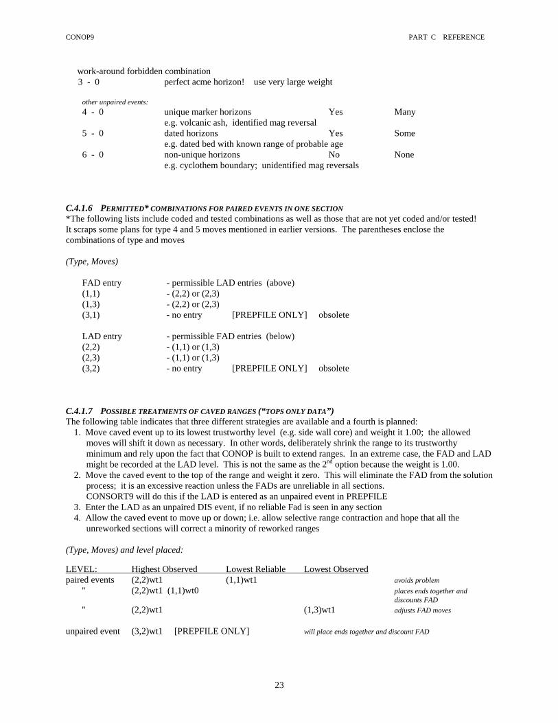
CONOP9 PART C REFERENCE

23

work-around forbidden combination 3 - 0 perfect acme horizon! use very large weight

other unpaired events: 4 - 0 unique marker horizons Yes Many e.g. volcanic ash, identified mag reversal 5 - 0 dated horizons Yes Some e.g. dated bed with known range of probable age 6 - 0 non-unique horizons No None e.g. cyclothem boundary; unidentified mag reversals

C.4.1.6 PERMITTED* COMBINATIONS FOR PAIRED EVENTS IN ONE SECTION *The following lists include coded and tested combinations as well as those that are not yet coded and/or tested! It scraps some plans for type 4 and 5 moves mentioned in earlier versions. The parentheses enclose the combinations of type and moves (Type, Moves)

FAD entry - permissible LAD entries (above) (1,1) - (2,2) or (2,3) (1,3) - (2,2) or (2,3) (3,1) - no entry [PREPFILE ONLY] obsolete LAD entry - permissible FAD entries (below) (2,2) - (1,1) or (1,3) (2,3) - (1,1) or (1,3) (3,2) - no entry [PREPFILE ONLY] obsolete

C.4.1.7 POSSIBLE TREATMENTS OF CAVED RANGES (“TOPS ONLY DATA”) The following table indicates that three different strategies are available and a fourth is planned:

1. Move caved event up to its lowest trustworthy level (e.g. side wall core) and weight it 1.00; the allowed moves will shift it down as necessary. In other words, deliberately shrink the range to its trustworthy minimum and rely upon the fact that CONOP is built to extend ranges. In an extreme case, the FAD and LAD might be recorded at the LAD level. This is not the same as the 2nd option because the weight is 1.00.

2. Move the caved event to the top of the range and weight it zero. This will eliminate the FAD from the solution process; it is an excessive reaction unless the FADs are unreliable in all sections. CONSORT9 will do this if the LAD is entered as an unpaired event in PREPFILE

3. Enter the LAD as an unpaired DIS event, if no reliable Fad is seen in any section 4. Allow the caved event to move up or down; i.e. allow selective range contraction and hope that all the

unreworked sections will correct a minority of reworked ranges (Type, Moves) and level placed: LEVEL: Highest Observed Lowest Reliable Lowest Observed paired events (2,2)wt1 (1,1)wt1 avoids problem " (2,2)wt1 (1,1)wt0 places ends together and

discounts FAD " (2,2)wt1 (1,3)wt1 adjusts FAD moves unpaired event (3,2)wt1 [PREPFILE ONLY] will place ends together and discount FAD

CONOP9 PART C REFERENCE

24

C.4.1.8 POSSIBLE TREATMENTS OF REWORKED RANGES (BASES ONLY DATA) The following table indicates that three different strategies are available and a fourth is planned:

1. Move reworked event down to its lowest trustworthy level and weight it 1.00; the allowed moves will shift it up as necessary.

2. Move the reworked event to the bottom of the range and weight it zero to eliminate it from the solutions process. Do this if there are no reliable observations of the LAD in any other section. CONSORT9 will do this if the FAD is entered as an unpaired event in PREPFILE

3. Enter the FAD as an unpaired APP, if no section has reliable LAD 4. Allow the caved event to move up or down; i.e. allow selective range contraction and hope that all the

unreworked sections will correct a minority of reworked ranges. (Type, Moves) and level placed LEVEL: Lowest Observed Highest Reliable Highest Observed paired event (1,1)wt1 (2,2)wt1 avoids problem! " (1,1)wt1 (2,2)wt0 places ends together and discounts

LAD " (1,1)wt1 (2,3)wt1 adjusts LAD moves unpaired event (3,1)wt1 [PREPFILE ONLY] CONOP9.CFG will place ends together and discount LAD C.4.1.9 POSSIBLE TREATMENTS OF CAVED-&-REWORKED RANGES The table below shows four strategies:

1. Shrink the observed range to its reliable minimum and weight the events 1.00. 2. Leave the range ends as observed and weight them 1.00, but allow them to move up or down section in order

to fit the more reliable information form other sections. This is pointless unless the unreliable ranges are a small minority of the data.

3. Leave the range ends as observed, allow them to move up or down section, and set the weights to zero so that these observations do not influence the solution process.

4. Enter the FAD and LAD as unpaired events that move up and down (-3,3) (Type, Moves) and level placed LEVEL: Highest-Obs'd Highest-Rel. Lowest-Rel. Lowest-Obs'd paired events (2,2)wt1 (1,1)wt1 " (2,3)wt1 (1,3)wt1 " (2,2)wt0 (1,1)wt0 C.4.2 FORMAT FOR "SECTFILE" ASCII format; fields separated by blanks within records; records separated by a carriage return. The first column is a sorted, unbroken set of section numbers that must match the numbers in LOADFILE. The third column sorts the same set of numbers into the order that the sections are to be plotted in fence diagrams. The second column is a 3-character nickname for fitting into tight spaces on graphics screens. The fourth column is the “full” name. The fifth column indicates whether (1) or not (0) the section should be used for the spacing task and construction of the composite section.

1 'Chi' 9 'Chilca Shale' 1

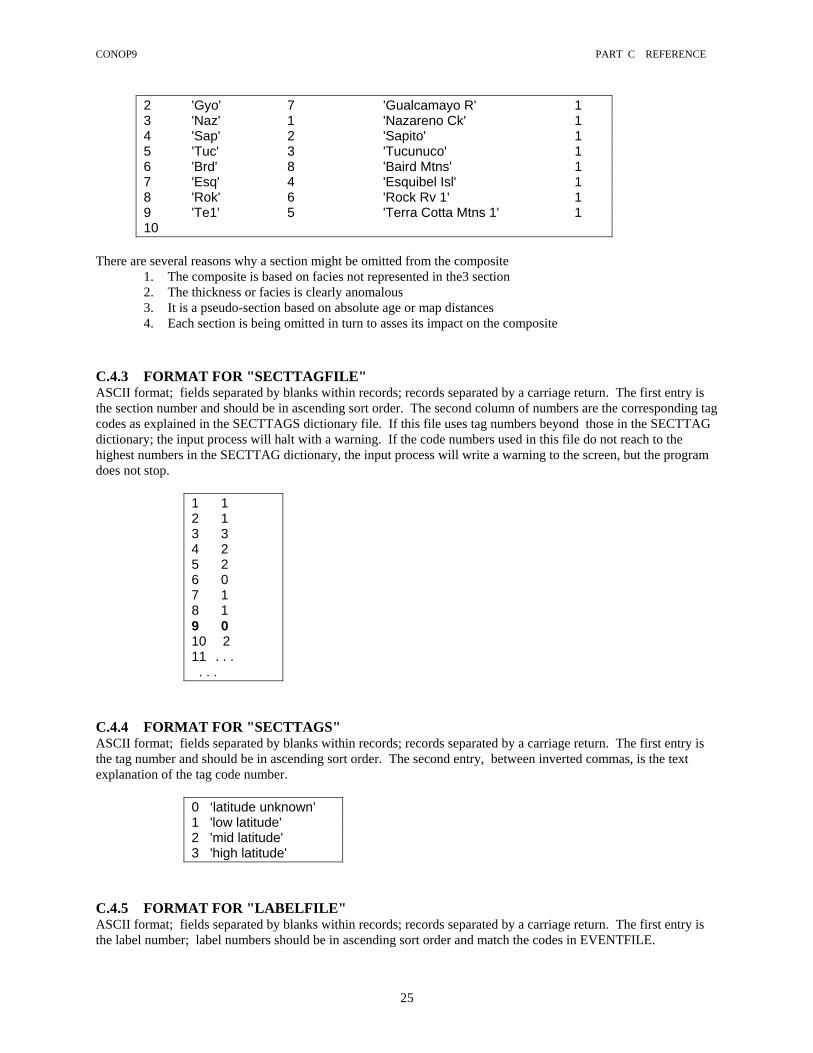
CONOP9 PART C REFERENCE

25

2 'Gyo' 7 'Gualcamayo R' 1 3 'Naz' 1 'Nazareno Ck' 1 4 'Sap' 2 'Sapito' 1 5 'Tuc' 3 'Tucunuco' 1 6 'Brd' 8 'Baird Mtns' 1 7 'Esq' 4 'Esquibel Isl' 1 8 'Rok' 6 'Rock Rv 1' 1 9 'Te1' 5 'Terra Cotta Mtns 1' 1 10

There are several reasons why a section might be omitted from the composite

1. The composite is based on facies not represented in the3 section 2. The thickness or facies is clearly anomalous 3. It is a pseudo-section based on absolute age or map distances 4. Each section is being omitted in turn to asses its impact on the composite

C.4.3 FORMAT FOR "SECTTAGFILE" ASCII format; fields separated by blanks within records; records separated by a carriage return. The first entry is the section number and should be in ascending sort order. The second column of numbers are the corresponding tag codes as explained in the SECTTAGS dictionary file. If this file uses tag numbers beyond those in the SECTTAG dictionary; the input process will halt with a warning. If the code numbers used in this file do not reach to the highest numbers in the SECTTAG dictionary, the input process will write a warning to the screen, but the program does not stop.

1 1 2 1 3 3 4 2 5 2 6 0 7 1 8 1 9 0 10 2 11 . . . . . .

C.4.4 FORMAT FOR "SECTTAGS" ASCII format; fields separated by blanks within records; records separated by a carriage return. The first entry is the tag number and should be in ascending sort order. The second entry, between inverted commas, is the text explanation of the tag code number.

0 ‘latitude unknown’ 1 'low latitude' 2 'mid latitude' 3 'high latitude'

C.4.5 FORMAT FOR "LABELFILE" ASCII format; fields separated by blanks within records; records separated by a carriage return. The first entry is the label number; label numbers should be in ascending sort order and match the codes in EVENTFILE.

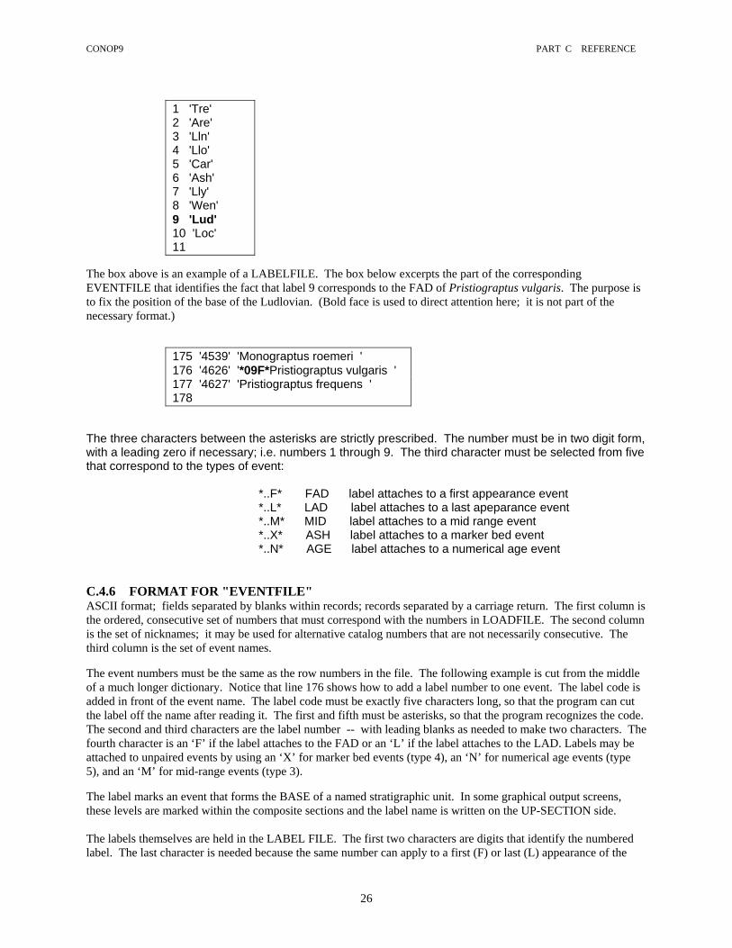
CONOP9 PART C REFERENCE

26

1 'Tre' 2 'Are' 3 'Lln' 4 'Llo' 5 'Car' 6 'Ash' 7 'Lly' 8 'Wen' 9 'Lud' 10 'Loc' 11

The box above is an example of a LABELFILE. The box below excerpts the part of the corresponding EVENTFILE that identifies the fact that label 9 corresponds to the FAD of Pristiograptus vulgaris. The purpose is to fix the position of the base of the Ludlovian. (Bold face is used to direct attention here; it is not part of the necessary format.)

175 '4539' 'Monograptus roemeri ' 176 '4626' '*09F*Pristiograptus vulgaris ' 177 '4627' 'Pristiograptus frequens ' 178

The three characters between the asterisks are strictly prescribed. The number must be in two digit form, with a leading zero if necessary; i.e. numbers 1 through 9. The third character must be selected from five that correspond to the types of event: *..F* FAD label attaches to a first appearance event *..L* LAD label attaches to a last apeparance event *..M* MID label attaches to a mid range event *..X* ASH label attaches to a marker bed event *..N* AGE label attaches to a numerical age event C.4.6 FORMAT FOR "EVENTFILE" ASCII format; fields separated by blanks within records; records separated by a carriage return. The first column is the ordered, consecutive set of numbers that must correspond with the numbers in LOADFILE. The second column is the set of nicknames; it may be used for alternative catalog numbers that are not necessarily consecutive. The third column is the set of event names. The event numbers must be the same as the row numbers in the file. The following example is cut from the middle of a much longer dictionary. Notice that line 176 shows how to add a label number to one event. The label code is added in front of the event name. The label code must be exactly five characters long, so that the program can cut the label off the name after reading it. The first and fifth must be asterisks, so that the program recognizes the code. The second and third characters are the label number -- with leading blanks as needed to make two characters. The fourth character is an ‘F’ if the label attaches to the FAD or an ‘L’ if the label attaches to the LAD. Labels may be attached to unpaired events by using an ‘X’ for marker bed events (type 4), an ‘N’ for numerical age events (type 5), and an ‘M’ for mid-range events (type 3). The label marks an event that forms the BASE of a named stratigraphic unit. In some graphical output screens, these levels are marked within the composite sections and the label name is written on the UP-SECTION side. The labels themselves are held in the LABEL FILE. The first two characters are digits that identify the numbered label. The last character is needed because the same number can apply to a first (F) or last (L) appearance of the

CONOP9 PART C REFERENCE

27

numbered taxon, or a mid-range (M) event. The X and N characters are included for symmetry and to allow for future developments that might need to use the particular nature of these event types.

167 '4499' 'Pristiograptus dubius parvus" ' 168 '4501' 'Gothograptus nassa ' 169 '4502' 'Colonograptus? praedeubeli ' 170 '4503' 'Colonograptus? deubeli ' 171 '4506' 'Neodiversograptus nilssoni ' 172 '4517' 'Bohemograptus bohemicus sl ' 173 '4518' 'Saetograptus fritsche linearis ' 174 '4521' 'Colonograptus colonus ' 175 '4539' 'Monograptus roemeri ' 176 '4626' '*09F*Pristiograptus vulgaris ' 177 '4627' 'Pristiograptus frequens ' 178 '4717' 'Pristiograptus pseudodubius ' 179 '4008' 'Araneograptus pulchellus ' 180 '4046' 'Kiaerograptus supremus ' 181 '4051' 'Tetragraptus phyllograptoides ' 182 '4092' 'Tetragraptus acclinans ' 183

The previous example used catalog numbers for the nickname. Abbreviated names are another possibility:

168 'Got.nass' 'Gothograptus nassa ' 169 'Col.prae' 'Colonograptus? praedeubeli ' 170 'Col?deub' 'Colonograptus? deubeli ' 171 'Neo.nils' 'Neodiversograptus nilssoni ' 172 'Boe.bohe' 'Bohemograptus bohemicus sl ' 173

Within the FORTRAN code and arrays, all events are assigned consecutive numbers. Paired events are numbered after unpaired events, with the FAD and LAD (+/-MID) assigned different numbers. Thus, the internal FORTRAN numbers reach higher values and do not correspond to any of the input numbers. Some of the CONOP9 output identifies these FORTRAN numbers. They are needed to predict the effect of the ‘STARTEVENT’ parameter. C.4.7 FORMAT FOR "EVENTTAGFILE" ASCII format; fields separated by blanks within records; records separated by a carriage return. The first entry is the event number and should be in ascending sort order, corresponding to the EVENTFILE. The second column of numbers are the corresponding tag codes as explained in the EVENTTAGS dictionary file. If this file uses tag numbers beyond those in the EVENTTAG dictionary; the input process will halt with a warning. If the code numbers used in this file do not reach to the highest numbers in the EVENTTAG dictionary, the input process will write a warning to the screen, but the program does not stop.

1 1 2 1 3 3 4 2 5 2

CONOP9 PART C REFERENCE

28

6 0 7 1 8 1 9 0 10 2 11. . . . . .

C.4.8 FORMAT FOR "EVENTTAGS" ASCII format; fields separated by blanks within records; records separated by a carriage return. The first entry is the tag number and should be in ascending sort order. The second entry, between inverted commas, is the text explanation of the tag code number.

0 ‘family unknown’ 1 'alphaidae' 2 'betaidae' 3 'gammaidae' 4 . . . .

CONOP9 PART C REFERENCE

29

C.5 COMMAND REFERENCE Notes: The order and grouping of commands matches CONOP9.CFG The configuration file lines appear in Arial Bold Narrow Font. C.5.1 PARAMETERS THAT IDENTIFY THE INPUT DATA ( &GETINN /) C.5.1.1 PROJECT = ['CHARACTER STRING IN INVERTED COMMAS'] Up to 60 characters in a project name that will be used as title for screen graphics. No effect on the optimization. C.5.1.2 SECTIONS = [INTEGER EQUAL TO NUMBER OF SECTIONS IN THE INPUT FILE] CONOP9 will halt with error message if this is incorrect. Array sizes are determined by this number. Of course, CONOP.EXE could determine this number while reading in the data; requiring that SECTIONS (and TAXA, and EVENTS) be stipulated independently serves as a safeguard that the correct data set is used and that the input files are complete. C.5.1.3 TAXA = [INTEGER EQUAL TO NUMBER OF TAXON RANGES (PAIRED EVENTS) IN THE INPUT FILE] CONOP9 will halt with error message if this is incorrect. Array sizes are determined by this integer number. Top-only and bottom-only taxa also count as one taxon; CONSORT9.EXE expands them to an event pair by plotting both range ends at the same horizon and weighting the missing end 1/10 of the reliable end. CONSORT9 can be used to edit the weights to another value if desired. If the weight is set to 0.00 the event will not be omitted from some output summaries. NOTE that the value of TAXA is the number of TYPE 1 events (same as the number of TYPE 2 events) in

LOADFILE. MID events (type 3) do not count because, like type 2) they must accompany a type 1. If counting from PREPFILE, include type 3 events with moves of type 1 or 2, for which there is no paired event in any section, because these events are expanded by CONSORT into a FAD and a LAD.

Each full taxon range makes 2 or 3 events (a FAD and a LAD plus-or-minus a MID), even if one of these events is not observed, but counts as only one taxon. Unpaired appearances and disappearances do not count into the TAXA total, even if they are taxon appearances and even if both the APP and DIS are included. CONOP does not make a taxon range unless the type 1 and type 2 events are paired.

To avoid any possible confusion with colloquial uses of "first" during drilling: the FAD is the "base" or "oldest" end of the taxon range.

C.5.1.4 EVENTS = [INTEGER EQUAL TO NUMBER OF 'OTHER' EVENTS IN THE INPUT FILE] 'Other' events are all unpaired events except the top-only and bottom-only ranges which must be expanded by CONSORT9 prior to running CONOP9. CONOP9 will halt with error message if it is supplied with a number for events which does not match its own inventory of the input files. Array sizes are determined by this number. Ash beds, radiometric dates, unpaired mid-range events, and the like are the unpaired events; they are never matched with a corresponding range end. The total number of paired and unpaired events that must be placed in sequence will be EVENTS + 2*(TAXA).

CONOP9 PART C REFERENCE

30

All events of 0<type<3 count as unpaired other events; i.e. –3, -2, -1, 0, 3, 4, 5, 6. Note that MID events (type 3) count as unpaired even though they require the accompanying types 1 and 2. Why? It is necessary because the rule is not reversible. Upon encountering a type 3 event, the program may assume that there will be a type 1 and a type 2 with the same number; but, encountering types 1 or 2 does not mean that there must be a type 3. C.5.1.5 MAX_LEVEL = [INTEGER EQUAL TO LIMIT ON THE NUMBER OF EVENT LEVELS IN A SINGLE SECTION] Integer may exceed the actual numbers without causing error. Setting this number too high wastes memory and might slow the run if memory is limited; a low setting causes run-time errors. It is very rare that a single section will have more than 150 different collecting levels with first and last occurrence events. NOTE that the composite sections may have many more levels than the actual field sections. For this reason they are stored in a separate array that is NOT limited by MAX_LEVEL C.5.1.6 MAX_LABEL = [INTEGER EQUAL TO LIMIT ON THE NUMBER OF STRATIGRAPHIC UNIT LABELS] Integer may exceed the actual numbers without causing error. Setting this number too high wastes memory and might slow the run if memory is limited; a low setting causes run-time errors. It is unlikely that more than 15 labels will be useful because there is not much room to print all the labels within a section. C.5.1.7 LOADFILE = [PATH AND NAME OF THE SORTED FILE WITH ALL THE LOCAL STRATIGRAPHIC DATA] Path and name must be enclosed in single quotes e.g. 'C:\camb\palmer.dat' Each record (line) in this file is one local observation. This file must have the record structure given at the bottom of these editing instructions and must be properly sorted on the first three fields. The maximum size of the input instance of the problem was fixed by the upper bounds of the arrays in CONOP3 and these were set at compile time. The limits were displayed on screen when CONOP3 was run. CONOP9 sets array sizes dynamically at run time the arrays are made just large enough to accommodate the number of sections and taxa supplied; the upper limit is determined by available memory LOADFILE is not optional! A valid filename must be supplied; and it must contain the appropriate

material. Conop9 will identify many formatting errors and inconsistencies in the contents of LOADFILE

C.5.1.8 PREPFILE = [PATH AND NAME OF AN UNSORTED VERSION OF THE LOADFILE] PREPFILE is sorted and completed by CONSORT9.EXE. In this file there is one record per observation, but the records may be in any order. Thus, the PREPFILE may be used for direct entry of records - one for each locally observed event. The levels (see below) may all be entered as zeros, or any integer, or even a blank space. CONSORT9.EXE will enter the proper level values; it offers two sort options: one for files without level integers and one for files with arbitrary level numbers; if the wrong option is selected, the LOADFILE will be corrupted; but it is a simple matter to repeat the call to CONSORT9 and get it right the second time. CONSORT9 does not alter the PREPFILE. Top-only and bottom-only taxon datums may be entered in this file and will be expanded by CONSORT9.EXE. PREPFILE is not needed by CONOP9.EXE.

CONOP9 PART C REFERENCE

31

C.5.1.9 SECTFILE = [PATH AND NAME OF FILE WITH SECTION NAMES] This is the optional section dictionary, keyed to the section number codes in LOADFILE. It is used in output text file and screen graphics for labeling. Format of each record in file must have the five items as follows: number 'nickname' position-in-fence 'full name' include?

nickname - no longer than 3 letters e.g. 'Btl' section numbers - integers in correct sequence position-in-fence - integer position from left to right in fence diagrams full name - no longer than 20 letters e.g. ' Bristol - Avon Gorge l' both names in single quotes include - two permitted integers, 1 or 0

all items separated by blanks all sections must be included the inclusion flag (column 5) was added in revisions to version 5. Earlier versions cannot handle this column The brevity of the nicknames may appear to be a nuisance. Ease of recognition is sacrificed in order to have a label short enough for crowded graphics where a full section name would not fit. The larger the data set, the more difficult the three-letter restriction becomes; yet it is the very large data sets that generate crowded graphics. If the SECTFILE is "OFF . . ." then CONOP simply reports its results in terms of section numbers. Section numbers must match the LOADFILE. Position-in-fence numbers are uniquely determined by this file. They may be changed from run to run. They must be the same set of integers used to label the sections, but may be listed in any order. Note that some word processors change the style of the inverted commas according to their position relative to other words. If these comma styles do not match between the beginning and the end of the names, CONOP may report an error during input. The error will report that a taxon number appears in the wrong line; if this is not the case, check the commas in the lines mentioned and up and down a few lines; because a mismatch causes the line-feed to be missed. The ‘include’ parameter determines whether the section thicknesses are used in the composite section and the spacing task. WARNING The include parameter was not part of the SECTFILE in early versions of CONOP9!! File not written if first three characters are 'OFF' Name may be added after OFF for ease of editing. [e.g. "OFFsect.dat" and "sect.dat"] C.5.1.10 SECTTAGFILE = [PATH AND NAME OF FILE WITH OPTIONAL SECTION TAGS] This is the optional file that attributes each section with a ‘tag’ number which must be keyed with the SECTTAGS dictionary. Tag codes are used to subdivide the diversity curves, for example, according to province. The information is deliberately stored in a separate file and NOT added as another column in SECTFILE. This decision allows older data sets to be run without modifying the SECTFILE. It also allows sections names and attributes to be used independently. We imagine that some users will create multiple tag files with names to indicate different section properties; e.g., climate, water depth, lithology. The format of each record must have the following two elements: section number tag code number Tag number 0 is used for unclassifiable section s, if any.

CONOP9 PART C REFERENCE

32

C.5.1.11 SECTTAGS = [PATH AND NAME OF FILE WITH SECTION TAG EXPLANATIONS] This is the section tag dictionary, keyed to the optional section tag numbers that are attached to the sections in the SECTTAGFILE. This file is NOT optional if the SECTTAGFILE is used. The format of each record must have the following two elements: tag number ‘tag explanation’ The first tag must be number 0 and is used to deal with unclassifiable sections, if any. The program code assumes that the first tag is 0 and will fail if this is not so! C.5.1.12 LABELFILE = [PATH AND NAME OF FILE WITH EVENT NAMES] This is the optional label dictionary, keyed to the optional event label numbers that are attached to some of the names in the event dictionary. The format of each record must have the following two elements: 'label number 'label name' C.5.1.13 EVENTFILE = [PATH AND NAME OF FILE WITH EVENT NAMES] This is the optional event dictionary, keyed to the event number codes in LOADFILE used in output text file. The format of each record must have the following three elements: 'nickname' event number 'full event name'

nickname - may be up to 8 letters; delimited with inverted commas; recommend 3 for genus and 4 for species: e.g. 'Har.falc'

the nickname may also be used to store a cross-reference code for custom databases that generate CONOP input files, such as the IGNS "Fossil Record" or Sadler's dBase system.

event number - integer corresponding to event number codes in LOADFILE full name - may be up to 50 letters; delimited with inverted commas; e.g. 'Harpoceras falcifer falcifer'

This file not read if first three characters are 'OFF'. File path and name may be added after OFF for ease of editing. [e.g. "OFFevnt.dat" and "evnt.dat"] In the absence of this file, CONOP will report events in terms of its internal event numbers. These are not keyed to taxa; the FAD and LAD have different numbers. Given a file of event names, CONOP will recognize those that are taxa and append "-FAD" and "-LAD" where appropriate. See notes under SECTFILE for matching commas. C.5.1.14 EVENTTAGFILE = [PATH AND NAME OF FILE WITH OPTIONAL EVENT TAGS] This is the optional file that attributes each event with a ‘tag’ number which must be keyed with the EVENTTAGS dictionary. Tag codes are used to subdivide the diversity curves, for example, according to family. The information is deliberately stored in a separate file and NOT added as another column in EVENTFILE. This decision allows older data sets to be run without modifying the EVENTFILE. It also allows event names and attributes to be used independently. We imagine that some users will create multiple tag files with names to indicate different event properties; e.g. taxon family, ecology. The format of each record must have the following two elements: event number tag code number Tag number 0 is used to deal with unclassifiable events, if any.

CONOP9 PART C REFERENCE

33

C.5.1.15 EVENTTAGS = [PATH AND NAME OF FILE WITH EVENT TAG EXPLANATIONS] This is the event tag dictionary, keyed to the optional event tag numbers that are attached to the events in the EVENTTAGFILE. This file is NOT optional if the EVENTTAGFILE is used. The format of each record must have the following two elements: tag number ‘tag explanation’ The first tag must be number 0 and is used to deal with unclassifiable events, if any. The program code assumes that the first tag is 0 and will fail if this is not so! C.5.1.16 BESTKNOWN = [DECIMAL VALUE OF BEST KNOWN PENALTY FOR THIS INSTANCE OF THE PROBLEM] Enter 0 or 0.0, if not known. CONOP will report if this value is not within 0.01 of the lowest value in CURVFILE -- this serves as a check that the input list items are compatible (easier than rummaging around in a big CURVFILE). This value may be used as an option to mark the expected minimum in graphical output and run-time graphics. This value does not influence the optimization. C.5.2 PARAMETERS THAT ALTER THE BEST SOLUTION ( &GETANS /) PRIMARY MEASURES OF MISFIT BETWEEN OBSERVATIONS AND SOLUTION The stratigraphic correlation problem includes three separable tasks: the sequencing task - place a set of events in the best sequence the spacing task - determine the relative spacing between events the locating task - identify, in each section, the horizon that corresponds in age with each event. The sequencing task must be completed in order to attempt the other two. The solution to the sequencing task is purely ordinal. The spacing task refers to a time scale that is uniform for all sections. The locating task is completed in local scales of stratigraphic thickness. In practice, the true solution is not knowable. The quality of solutions must be measured by the misfit between observations and solutions. Several measures of misfit are available; they will typically give rise to different answers; and the choice must be guided by the nature of the data and the purpose for which the answer will be used. The analogy with linear regression is very close. SOME JARGON: In optimization problems, the misfit is termed the "penalty" or the "cost," if it is minimized. The algebraic formulation of the misfit is termed the "objective function." Aspects of the task or solution that concern only one section are termed "local." Aspects of the solution that apply to the whole data set are termed "global." Note that the "global" sequence would then refer to a sequence fit to the entire input data set, but not to some global zonation scheme involving data outside the current instance of the problem; i.e. "global" is used in its computer science sense, not in its geographic _ sense of "world-wide". TWO OPTIMIZATIONS: The sequencing task is always attempted first, otherwise there is no correlation in any sense. The locating task is necessary for some measures of misfit. When the locating and sequencing tasks are attempted together, there are two optimizations:

CONOP9 PART C REFERENCE

34

1. The "outer optimization" finds the sequence with the best fit. In CONOP9 the outer optimization is always a heuristic search. 2. The "inner optimization" finds the best placement of events in sections for any sequence that arises in the outer search. It solves the locating task. In CONOP9 the inner optimization is always a deterministic process, building the placements section-by-section and from the bottom up. Events treated in the order of the current sequence, from oldest to youngest and are placed from bottom to top. As the stack of placements is built up for each section, successive events are placed at the top of the stack or at the observed level, whichever is the higher. The stack is compressed when necessary to minimize the penalty. MISFIT MEASURES Three distinctly different forms of misfit are considered. They become evident when one adjusts the local ranges to fit the global sequence: 1. Misfit based on the length of range extensions – a fitting of observations to trial sequences The lengths of the locally observed ranges must be adjusted and this gives rise to natural interval increments of misfit that can be summed across all observed range ends and all sections. INTERVAL and LEVEL options for PENALTY are alternative ways to measure this type of misfit (see entries below). Combined with a constraint against range contractions, these measures cause the search to match the economy-of-fit principle formulated by Shaw (1964), and seek maximal ranges (from the earliest FAD to the latest LAD). These are the ranges needed for paleobiological studies and for establishing world-wide zonal schemes. 2. Misfit based on the pairwise contradictions in the order of events – a comparison of trial and observed sequences Some locally observed sequences of pairs of events will be contradicted as the ranges are adjusted. It is precisely this kind of contradiction between sections that generates the correlation problem. Thus, ordinal penalties arise naturally from the number, size, and relative frequency of contradictions. They must be summed across all observed pairs of events and all sections. ORDINAL, SPATIAL, and RASCAL options for PENALTY are alternative ways to measure this type of misfit. If the penalty against range contractions is relaxed, these options can find the average observed range. The result can be a prediction of the most likely observed sequence of events in a new section or well. 3. Misfit based on excesses in the trial sequences relative to observed constraints. The observed sequences establish constraints in the form of pairs of taxa that must co-exist and first appearances that must be placed before the last appearances of other taxa. Viable trial sequences typically require (imply) more coexistences and more pairwise orderings. We may attempt to minimize these. The ROYAL option for PENALTY measures misfit as the number of implied but unobserved pairwise coexistences of taxa. The SEQUEL option for PENALTY measures misfit as the number of implied but unobserved pairwise orderings of first appearances below last appearances. The ROYAL penalty is a subset of the SEQUEL penalty. Measures of misfit in categories 2 and 3 can often be used in faster algorithms than CONOP9, because they do not perform the inner optimization. They are included here in order to emulate other methods, to ensure that differences are not due to the optimization procedure, to enable mapping of the set of equally well-fit solutions, and to enable these measures to be applied with a wider tolerance for events of different type. C.5.2.1 PENALTY = 'LEVEL' | ‘INTERVAL’ |’EVENTUAL’ | ‘ORDINAL’ | ‘SPATIAL’ | ‘RASCAL’ | ‘ROYAL’ / ’SEQUEL’ PENALTY = 'LEVEL' The LEVEL penalty is based on range extensions and measured in numbers of event levels -- the number of event levels that lie in the range extension and are “leapfrogged” as the observed range end is moved to the far end of the range extension. This removes the influence of differences in accumulation rate from section to section. INTERVAL tends to favor the sequences seen in the thickest sections; wide sample spacing may exaggerate this bias.

CONOP9 PART C REFERENCE

35

LEVEL tends to favor the sequences seen in the sections with the most rich and diverse fossil biotas; of course, close sample spacing is necessary to capture this richness. Like INTERVAL, this setting also completes the location task in order to measure the misfit between the global sequence and the local observations. Although INTERVAL was the original form of the penalty (Kemple et al. 1995), most instances of the problem perform well with LEVEL and some only perform well with level. When the sections include a mixture of different facies types and accumulation rates, it is probably better to run with the LEVEL penalty. The LEVEL and EVENTUAL penalties emulate some features of Edwards’ “no-space graphs” in the sense that they focus on order rather than the thickness interval between events. The INTERVAL penalty would come closest to mimicking Shaw’s graphic correlation. Calculation of the level penalty requires solving both the sequencing task and the location task. PENALTY = 'EVENTUAL' The EVENTUAL penalty is based on range extensions and measured in numbers of events -- the number of events that lie in the range extension and are “leapfrogged” as the observed range end is moved to the far end of the range extension; i.e. an event level that includes more than one event will add more than one to the penalty. This removes the influence of differences in accumulation rate from section to section. More so than LEVEL, EVENTUAL tends to favor the most richly fossiliferous sections by counting all range ends (events) that are leapfrogged, not just the levels involved. Calculation of the EVENTUAL penalty requires solving both the sequencing task and the location task. This makes it slower than the ORDINAL penalty. But EVENTUAL counts only the range extensions necessary to reverse all contradictory pairs; ORDINAL counts all contradicted pairs. A contradiction can be eliminated by bringing two events to the same level, then they are consistent with any order. ORDINAL counts all the contradictions. The EVENTUAL penalty resembles the ORDINAL penalty; but is less efficient to calculate. In version 6.2, expect the EVENTUAL penalty to be of the same order of magnitude, but sometimes larger than the ORDINAL penalty. Starting with version 6.3, expect the EVENTUAL penalty to be of the same order of magnitude, but smaller than the ORDINAL penalty. It is a matter of whether or not to count the events at the levels from which and to which the event is moving. Starting with 6.3, these events at the end of the move are ignored. That is, because the local section cannot discriminate the order of events at one level, no EVENTUAL penalty is assigned for apparent ties, regardless of the model order of events. ORDINAL discriminates the events at the new level, between those above and those below, adding a penalty for those overstepped by the model sequence. Actually, once the event is placed at the new level, its order with respect to events at the same level is treated as equivocal, its order with respect to events at the observed level is now decided. Thus, for a move of one level up or down, the eventual penalty is conventionally 1.0; the moving event has stepped over itself, but no other overstepping can be proven. For moves of more than 1 level, the eventual penalty is 1.0 plus the total of events at all the leapfrogged levels. It is a subtle point. Perhaps both options should be available; they could be tied to the setting for FORCECOEX, because it is a matter of the interpretation of the relative age of events found at the same level. To the extent that surfaces of hiatus and omission tend to concentrate range ends, EVENTUAL imparts a reluctance to extend ranges over hiatuses. The EVENTUAL penalty was introduced late and, as a result, has been little used. It might appear to be the most sequence-stratigraphically enlightened penalty. One could imagine adding dummy events to surfaces of hiatus in numbers proportional to the perceived magnitude of the hiatus. From another point of view, the EVENTUAL penalty reveals a fundamental shortcoming of the ordinal measures of misfit (ORDINAL and RASCAL) -- they do not measure a property of misfit that relates naturally to preservation and recovery of fossils. Misfit is attributed to failures of preservation and recovery of fossils. Misfit is surely more remarkable when it is implied to extend over thicker stratigraphic intervals and more intensely sampled intervals. It is not necessarily relevant to know whether the interval of misfit contains the ends of many other taxon ranges -- this is only an indirect guide to preservation potential in that interval.

CONOP9 PART C REFERENCE

36

The EVENTUAL and LEVEL penalties emulate some features of Edwards’ “no-space graphs” in the sense that they focus on order rather than the thickness interval between events. The INTERVAL penalty would come closest to mimicking Shaw’s graphic correlation. PENALTY = 'INTERVAL' The INTERVAL penalty is based on range extensions and measured in stratigraphic thickness between observed and placed event horizons: the sum of all range extensions across all taxa and all sections i.e. Shaw's economy-of-fit. This penalty often seems to be the easiest for a beginner to grasp, especially those familiar with graphic correlation. Nevertheless, the LEVEL penalty or, perhaps, the EVENTUAL penalty is likely to be a more versatile and trustworthy measure of misfit. INTERVAL tends to favor the sequences seen in the thickest sections. Like LEVEL, this setting also completes the location task in order to measure the misfit between the global sequence and the local observations. The INTERVAL penalty would come closest to mimicking Shaw’s graphic correlation. The LEVEL and EVENTUAL penalty emulate some features of Edwards’ “no-space graphs” in the sense that they focus on order rather than the thickness interval between events. The INTERVAL penalty is measured on a continuous scale. It can be applied to any such scale. Obviously, a time scale would work. Less obviously, a scale might be based upon the abundance of fossil faunas. That is, distance could be measured up-section as a total count of fossil finds. The logic would be to extend ranges more readily through intervals that yielded sparse fossils than through intervals that preserve abundant fossils. Calculation of the interval penalty requires solving both the sequencing task and the location task. PENALTY = 'ORDINAL' The ORDINAL penalty measured by NUMBER of contradictory pairwise event orderings i.e. a democratic ordering like RASC and Hay's method; ORDINAL tends to produce shortened ranges, so LETCONTRACT = 'ON' to mimic Hay's method (but, see warnings under LETCONTRACT). If BOTH weight-up and weight-down are set to zero, the event is excluded from this penalty. This measure does not require the location task. It therefore permits a faster search than an interval penalty; but the locating task must be completed subsequently by applying an interval measure of misfit to the best sequence found by the ordinal penalty. This option is fit to the annealer arrays and solved by inversion/simulated annealing, which is not optimal for this method. Crampton et al. (2001) make the important observation that democratic ordering answers the question: if I measure another section or drill another well in the same region, what sequence of events am I most likely to encounter? Methods that seek the extreme range ends (graphic correlation, INTERVAL, LEVEL, EVENTUAL) answer a different question: what is the net sequence of events for the region as a whole. Because ORDINAL implies that observed ranges are equally likely to be too short or too long, it is less likely to be compromised by local instances of reworking. Of course, this is a rather extreme precaution against reworking. The other extreme is to assume that it is not present in the data set (INTERVAL, LEVEL, EVENTUAL). PENALTY = 'SPATIAL' The 'SPATIAL' penalty measured by SIZE of contradictory pairwise event orderings. Also ordinal, but the size of the contradiction is measured by the number of intervening levels, i.e. a large contradictory separation is penalized more heavily. If BOTH weight-up and weight-down are set to zero, the event is excluded from this penalty. This option is fit to the annealer arrays which are not optimal for this method.

CONOP9 PART C REFERENCE

37

Notice that this measure will use the local stratigraphic separation of two OBSERVED events whose local order is contradicted by the global solution. The INTERVAL and LEVEL penalties use the separation between an observed event and its best location according to the global solution. The INTERVAL and LEVEL penalties determine the smallest adjustments necessary to fit the local range chart to the global solution. One adjustment may “correct” several ordinal misfits. The SPATIAL penalty adds up all the ordinal misfits to be corrected, whether or not several may be corrected by a single adjustment. This measure does not require the location task. It therefore permits a faster search than an interval penalty; but the locating task must be completed subsequently by applying an interval measure of misfit to the best sequence found by the spatial penalty. PENALTY = 'RASCAL' The 'RASCAL' penalty measured by RELATIVE FREQUENCY of contradictory pairwise orderings observed; this is also ordinal, but the number of contradictions is expressed as a fraction of the total number of observed orderings for that event-pair. i.e. a crude attempt is made to be probabilistic like the RASC and Hay methods. If BOTH weight-up and weight-down are set to zero, the event is excluded from this penalty. This option is implemented by the annealer arrays which are not optimal for this method. For each pair of events, the penalty increment ranges from 0 (no contradictions) to 1.0 (all observations at odds with global solution) and, thus, resemble a probability. But the values for all pairs are simply summed; not corrected for the grand total of observed pairs. To find the latter measure of misfit, divide the ordinal penalty by half the number of contradictable events. Because this number is fixed for each instance of the problem; the ORDINAL penalty effectively provides this measure. This measure does not require the location task. It therefore permits a faster search than an interval penalty; but the locating task must be completed subsequently by applying an interval measure of misfit to the best sequence found by the spatial penalty. PENALTY = 'ROYAL' The 'ROYAL' penalty measures the excess number of coexistences implied by the solution, relative to the number confirmed by observations. This NOT likely to be the most viable penalty, on its own, for solving the correlation problem. It demonstrates the limited power of the coexistence constraints alone. It allows solutions with huge interval penalties, because there is no solution to the locating task that might stop range contractions. The best results from this penalty emerge in conjunction with the FORCEFb4L constraint, which provides a sense of polarity, if at least two faunas have known superpositional sequence. Of course, the FORCEFb4L constraint and the ROYAL penalty are subsumed in the SEQUEL penalty. ROYAL is included for historical reasons – to allow some emulation of the initial CONJUNCT program (Alroy, 1992). The initial random sequence places all FADs before all LADs. Thus, every possible FAD-before-LAD is realized and the initial ROYAL penalty should be the same, regardless of the internal ordering of the FADs and LADs. Coexistences are the primary data of the Unitary Associations methods (Guex, 1977, 1991; Alroy [anagram!], 1992). They permit the recognition of a series of assemblage zones. To use ROYAL in this way, it would be necessary to solve the locating task at each step and, thus, outlaw range contractions. ROYAL may be implemented as a secondary penalty by setting STACKER=’COEX.’ The combination of PENALTY=’ROYAL’ with FORCEFb4L=’ON’ provided the best approximation of the event-ordination method described by Alroy in 1994, until the SEQUEL option was provided (below). PENALTY = 'SEQUEL' The 'SEQUEL' penalty measures the excess number of FAD-before-LAD pairwise event orderings, relative to the number confirmed by observations. When the penalty function is measured in terms of range extensions, and range contractions are not permitted (LETCONTRACT=’OFF’), the FAD-before-LAD observations are automatically

CONOP9 PART C REFERENCE

38

honored. The results of the SEQUEL penalty might not satisfy users who seek a solution that reproduces the fine details of event separation seen in stratigraphic sections (as utilized by the INTERVAL and LEVEL penalties). But the SEQUEL penalty provides much faster solutions than the INTERVAL or LEVEL options: it does not need to read the individual section files during the search; and it does not need a secondary STACKER=’COEX’ penalty. Coexistences are subsumed by FAD-before-LAD observations. Estimates of the duration of a stratigraphic section tend to be systematically shorter with the SEQUEL penalty than with the LEVEL and INTERVAL penalties. Why? The SEQUEL penalty derives no sequence information from the run of first occurrences at the base of a section or the run of last appearances at the top of a section. SEQUEL draws its information only from observed intermixtures of first and last appearances. These runs of first occurrences at section bases and last occurrences at section tops are, in part, an inevitable artifact of extracting a portion of the longer stratigraphic record; they include real first occurrences (which do not change if the measured section is extended to include more strata) together with artificial range truncations (which would change if the section were extended). Thus, the SEQUEL penalty represents one extreme view – none of the observed relative positions in these runs of like events is useful. The LEVEL and INTERVAL penalties represent another extreme view – all of the observed relative positions are useful. Neither strategy is really quite so extreme; both hope that the data set includes enough sections that most time intervals fall within the span of a section more often than they fall at the top or base of a section. Notice, therefore, that both strategies are jeopardized by the systematists habit of truncating sections at the boundaries of major stratigraphic units. Fortunately, the process of global stratotype selection has encouraged the development of numerous short stratigraphic sections that span major unit boundaries. Taken together, the results of the two endeavors mitigate one-another’s shortcomings. The initial random sequence places all FADs before all LADs. Thus, every possible FAD-before-LAD is realized and the initial sequel penalty will be the same, regardless of the internal ordering of the FADs and LADs. The initial and final penalties tend to be 10x or more larger than the corresponding LEVEL penalty. One set of experiments found no need for a correspondingly large increase in the initial temperature. It appears that the SEQUEL penalty performs best with somewhat higher starting temperatures than the LEVEL and INTERVAL penalties. Certainly, it is more practical to raise the starting temperature when selecting a faster penalty. In summary, the SEQUEL option has two advantages with large data sets. It is fast and its results are likely to improve as the data set grows – fewer intervals will be seen exclusively near the ends of sections where first and last appearances are not intermixed. For large data sets with many taxa known only from single sections, cross plots of LEVEL and SEQUEL solutions show subsets of taxa with internally consistent ordering that interleave differently under the two objective functions. These subsets may represent different provinces. This penalty requires that the FORCEFb4L constraint be activated. The program does this automatically. The constraint builds a square array, with both dimensions equal to the number of taxa in the data set. For large data sets this additional array might strain the memory resources of limited hardware. FAD-below-LAD constraints are a key element of Alroy’s (1994, 2000) Appearance Event Ordination (AEO). Although the SEQUEL setting uses the logic of AEO, it does not mimic Alroy’s seriation method in detail. Alroy derives relative age indices for individual faunas and then builds a composite section from them. CONOP is section-based, not fauna-based. It corrects and completes the individual sections and builds composites from them. PENALTIES REPORTED IN OUTFILE AND AT LOG-OFF: Although the final solution is optimized for only one of the five measures of misfit, all five penalties can be calculated once the sequence is fixed by any means. So, the output reports all measures of misfit for the final sequence. PENALTIES USED FOR THE COMPOSITE SECTION:

CONOP9 PART C REFERENCE

39

Although the sequence of events in the composite section is determined by the user-specified measure of misfit, the composite section cannot be given stratigraphic thickness except by reference to local solutions of the locating task. This task is undertaken with an INTERVAL penalty in order to separate events by real stratigraphic thicknesses, regardless of the penalty type used to solve the sequencing problem. COMPOUND MISFIT MEASURES It appears evident that no single measure of misfit can capture all the aspects of discrepancy between data and solution. Compound measures of misfit can, theoretically, be generated by adding together different combinations of the five penalties discussed above. The summation could involve weighting functions to adjust the relative contributions of each term. Because this leads to a huge array of possible penalties, that would be difficult to analyze, it is not implemented. Just consider logistics of switching each penalty type off or on and, if on, providing a relative weight, in to grasp the proliferation of potentially different solutions to be analyzed! Nevertheless, the programming task is quite straightforward. Secondary measures of misfit are provided. They are not drawn from the above, but quantify aspects of the solution that are rather different. The secondary measures can be solved together with the primary measures during annealing or by applying a greedy algorithm after the primary measure has been minimized alone. Most of the secondary misfit measures were written in order to achieve acceptable solutions for seriation problems. When the secondary penalty is used for seriation, it usually carries a relative weight that is less than 1.00. Low weighting is necessary for a good solution but can lead to spurious high precision in the differences between nearly best misfit solutions. If this factor is a concern, it can be addressed through the relaxed fit curves. C.5.2.2 WEIGHTING

= 'FILE' | ‘ON’|'OFF' | ‘COEX%1’|’COEX%2’ | ‘COEX%5’ | ‘COEX%10’|’COEX%15’ | ‘COEX%20’ | ‘COEX^-1’|’COEX^-2’ | ‘COEX^-3’ | ‘COEX’|’COEX2’ | ‘COEX3’

[options to override the weight values in the input file]

WEIGHTING= 'ON'|’FILE’ Use the weights in the input files.

WEIGHTING= 'OFF' Ignore the weights in the input files; set all the stored values for program use to 1.00. WEIGHTING= ‘COEX%1’ | ‘COEX%2’ | ‘COEX%5’ | ’COEX%10’

| ‘COEX%15’ | ‘COEX%20’ Reduce the weights in the input files to one tenth of the listed weights for those taxa that are likely to have long ranges, based on the large numbers of observed/proven coexistences. Apply this adjustment to the given percentile (1, 2, 5, 10, 15, 20) with the largest number of coexistences. This is an attempt to prevent short segments of a long range from being correlated rather than stacked. These short partial ranges result when taxa have longer ranges than the stratigraphic sections or when long-ranged taxa from a subordinate environment appear in brief incursions into the dominant facies. The strategy works well when applied subjectively to taxa that are widely believed to suffer from this problematic distribution. The challenge is to apply something like it in an automated and reproducible manner. The file RUNLOG.TXT will list the names and/or numbers of taxa to which this weight reduction has been applied. The options listed below remain from an earlier, and often less successful, approach to the same problem.

WEIGHTING= ‘COEX^-1’|'COEX'

CONOP9 PART C REFERENCE

40

Ignore the weights in the input files. Set the weights for each taxon to the reciprocal of the number of observed coexistences. This is an attempt to give lower weights to longer ranging taxa, which tend to have more coexistences. The ploy seemed to have considerable merit for large seriation problems in which individual sections are often shorter than the longer taxon ranges. It tries to prevent short segments of a long range from being correlated rather than stacked. Unfortunately, the differential weighting seems to be too extreme and to extend to too many taxa. As a consequence, the program loses it grip on some large data sets and cannot converge on a good solution (see WARNING below). When WEIGHTING=’COEX’ the weighting factors are all less than 1.00 and all events are weighted. For large data sets, some weighting factors may be lower than 0.01. As a consequence, the value of the net penalty becomes much smaller and other adjustments may be necessary: the temperature settings during simulated annealing (see below) may need to be reduced; and the scaling factor for the secondary penalty may need to be reduced. WARNING: With very large data sets, it becomes apparent that COEX weighting may seriously diminish the ability of the annealing routine to complete the intermediate and fine-scale optimization. Presumably, it has rendered the landscape debilitatingly smooth by setting up too many equally misfit sequences. In order to reduce the weighing differential, try COEX2 or COEX3.

WEIGHTING= ‘COEX^-2’|'COEX2' Employs the same strategy as COEX, but uses the square-root of the number of observed coexistences. This is a more conservative weighting differential. It may counteract the tendency of COEX to smooth out the penalty landscape and prevent some searches from converging on an optimal solution in the later part of the search.

WEIGHTING= ’COEX^-3’| 'COEX3' Employs the same strategy as COEX, but uses the cube-root of the number of observed coexistences. This is a more conservative weighting differential. It may counteract the tendency of COEX to smooth out the penalty landscape and prevent some searches from converging on an optimal solution in the later part of the search.

C.5.2.3 EXCLUSIVES

= 'NO' | ‘YES’ [An additional misfit measure designed to constrain the placement of exclusive events]

EXCLUSIVES = 'NO' Do not take additional measures to control the placement of exclusive taxa. Either there are no exclusive taxa in the data set or there is no need to constrain their placement beyond the normal influence of coexisting taxa and position relative to shared taxa. EXCLUSIVES = 'YES' Take precautions to improve the placement of exclusive taxa in the sequence of events. The biggest problem with exclusive taxa arises when they are found above or below all the shared taxa in the section. Without penalty, these taxa can drift far above or below the true range of the section. EXCLUSIVE=’YES’ activates a preventive measure: add to the measure of misfit, the average span of events of all the sections that have exclusive events at the highest or lowest levels. As a dataset is loaded, CONOP9 lists all sections that have exclusive events at the top or base. The span of events of all these sections is added up with each trial sequence and divided by the number of such events. If there are no such events, the EXCLUSIVES setting is automatically set to “NO.” C.5.2.4 FORCEFB4L

= 'ON' | ‘OFF’ | ‘FILE’ [A Constraint]

FORCEFb4L = 'ON' This constraint does not accept solutions unless they honor all observed instances of First Appearance events occurring before (older than, below) Last Appearance events. This constraint may speed a search by restricting the

CONOP9 PART C REFERENCE

41

range of acceptable sequence mutations. It is most powerful as a source of polarity when PENALTY=’ROYAL’. In order to enforce this set of constraints, an additional array must be built. It has a row and a column for every taxon in the data set. If the number of taxa is large and computer memory (RAM) is in short supply, then activating this constraint may rob memory resources from other essential calculation. Thus, it can slow the search on some hardware configurations.

FORCEFb4L = 'OFF' Releases this constraint. Note that the constraint is implicit when the measure of misfit (PENALTY=) is based on range extensions and range contractions are prohibited (LETCONTRACT=’OFF’).

FORCEFb4L = 'FILE' Not tested. The option is intended to allow the user to edit the set of constraints. C.5.2.5 FORCECOEX

= 'SS' | ‘SL’ | ‘FILE’ [A Constraint]

FORCECOEX = 'SS' The “strict” coexistence criterion does not accept solutions unless they honor strictly proven coexistences of taxon pairs. Sensu stricto means that coexistence must be proved by overlapping range ends in a single section. We do not accept the indirect evidence derived from the more than one section (reversals of pairwise sequences of FADs or LADs) and we do not accept range ends in the same sample/horizon as evidence (the sample has finite thickness and the horizon might be condensed). [Regardless of the setting SS, SL, or OFF, the initial solution is made to honor all SL coexistences. Otherwise, initial penalties can be ridiculously high and some instances of the problem generate insoluble options that cause general protection errors. The coexistence matrix is rebuilt using the requested criterion as soon as the initial solution has been built. The initial phase of a CONOP9 run will echo these steps to the screen] [To view the proportions of SS and SL coexistences, run CONTROL9.EXE which plots the coex matrix and colors SS red and Sl blue] FORCECOEX = 'SL' Under the “loose” criteria for coexistence, solutions honor all coexistences, including those proven by coexistence in a single sample/horizon, and those proven by contradictions between sections. This setting ignores the possibility that some observed coexistences may be the result of "time averaging" in condensed shell beds. It may, therefore, stipulate a larger number of coexistences than 'SS,' thus increasing the constraints. As a result, the best solution may have a larger penalty. For large data sets with few internal contradictions, the settings SS and SL may produce the same coexistence table. [Range ends that are weighted 0.0 (for up AND down adjustments) do NOT count as proof of coexistences for either the SL or SS criteria. Thus, range ends that are tagged as reworked or caved may count as proof of coexistences unless BOTH weight-up and weight-down are "zeroed."] Notice that SL coexistence may be proven even if all FADs, or all LADs, are zeroed out by their weights. The proof derives from differences in the locally observed pairwise sequence from more than one section. Range ends that are neither caved nor reworked cannot be observed in contradictory order unless sampled from an overlapping portion of two ranges. Arguments that use two sections are, by definition, considered SL because comparison of two sections is inevitably prone to more sources of error than direct observation. The coexistences reported in the output from CONOP9 will reflect the setting of FORCECOEX. To see what difference the two criteria would make, use CONTROL9 which reports the highest level of coexistence criteria observed for all pairs of taxa.

CONOP9 PART C REFERENCE

42

FORCECOEX = 'OFF' Do not enforce observed coexistences in solutions FORCECOEX = 'FILE' Use the coexistences in the file identified by the COEXISTFILE parameter. Large instances of the problem may take so long to calculate the coexistence matrix that CONOP appears to have frozen during the start-up sequence (especially with slow hardware and early versions of CONOP9). The FILE option ensures that the matrix need only be built once. Use the “FILE” setting on subsequent runs with the same data set to save the time used to calculate the coexistence matrix. After version 3.3 of CONOP9, the routine that determines the coexistence matrix was radically accelerated; the FILE option was retained. This is a two-edged option. It allows the coexistence matrix to be edited, but it does not check to determine whether the edited file will cause run-time problems. To minimize such problems, the starting solution should be random and this is hard coded regardless of STARTYPE. The COEXISTFILE is not always easy to edit; it is symmetrical and may be large, having one row and one column for every taxon. But, CONOP builds and stores a suitable file (see COEXFILE=) in every run. Thus, the best use of 'FILE' is simply to reuse the machine-generated table, without editing. This will accelerate the second and subsequent runs of large data sets. Building a very large coexistence table will contribute significantly to the waiting time before the animated range chart starts; loading from file is quicker. The coexistence table is not re-built during the search (after the animated range-chart starts); so the setting of the FORCECOEX parameter does not influence the reported search time. C.5.2.6 LETCONTRACT

= 'OFF' | ‘ON’ | ‘FILE’ | ‘SS’ | ‘SL’ [A Constraint]

LETCONTRACT = 'OFF' The ‘OFF’ setting is standard; it prevents all ranges from contracting. This setting is not an absolute constraint; rather, it assigns a large weighting factor to penalty increments that involve contraction (x 7777). An absolute constraint might limit the interconnectivity of the neighborhood structure and allow the search to stall in very poor solutions. Notice that this setting has no impact unless the locating task is undertaken. The ROYAL penalty, for example, finds solutions that include range contractions in spite of LETCONTRACT. The LETCONTRACT parameter needs to be turned ON by one of the options below in order to generate a solution that resembles the so-called "average" ranges. Notice that average is usually a misnomer for the ranges. If anything is 'average' it is the position of the events in sequence; this does not necessarily generate an average range. Furthermore, the results of RASC and modified Shaw's methods are more likely to generate a 'modal' sequence -- the one most commonly preserved at individual sections or wells. LETCONTRACT = 'FILE' The 'FILE' option allows range contractions according to input file [overrule the input file without retyping it by using the following universal settings] LETCONTRACT = 'SL' The 'Sensu Lato' setting allows any range to shrink or shift totally outside the observed span i.e. allowed ranges as if allowed moves for LAD were ‘3’ and for FAD were 3.

CONOP9 PART C REFERENCE

43

LETCONTRACT = 'SS' The 'Sensu Stricto' setting allows any range to shrink but not shift, i.e. placed ends may move into the observed range but not through it. LETCONTRACT=”ON” DISCLAIMERS and WARNINGS DISCLAIMER: Settings other than 'off' have not been subjected to the extensive testing that the 'off' setting has passed. They might still generate unpredictable effects or program crashes in combination with some other parameter settings. The animated range chart might not handle shifting or shrinking ranges very elegantly. If Letcontract is “on” observed ranges may be shrunk to the point of eliminating all taxon coexistences and FAD-before-LAD event pairings. The ROYAL and SEQUEL penalties (objective functions) may tend to force the solution toward this extreme! If range contractions are allowed AND the observed coexistences are to be honored, then the coexistence table ought to be updated every time an observed range contracts! But the updating has not been coded in this version of CONOP9. In other words, if LETCONTRACT= “on” it is logical and advisable to turn off the coexistence and FAD-before-LAD constraints. One attractive feature of range contractions is the potential to eliminate rare instances of reworking or bad identifications. For this benefit to be realized, there must be a preponderance of good observations over the bad; in other words, all taxa should enjoy constraints from numerous observations, most of them good. For taxa known from only one section, the FORCECOEX and FORCEFb4L constraints serve to generate plausible ranges in the composite sequences. As explained, however, if LETCONTRACT=”ON” it is logical that these two constraints should be turned off. As a result, taxa that previously enjoyed some constraint are now free to assume implausible and almost random ranges in the best-fit solutions. Such random ranges are often long and can be particularly ridiculous in seriation problems where the timespan of the solution extends far beyondthe limits of any one section. The solution is severely compromised and estimates of species richness, for example, beome excessive. These long ranges may be unexpected because LETCONTRACT=”ON” tends to shorten the composite ranges of well-constrained taxa. Not surprisingly, the problem of poorly constrained taxa is similarly acute for the RASC algorithms, and the RASC guidelines encourage the culling of taxa that are observed in too few sections. C.5.2.7 HOMERANGE

= 'SS' | ‘SL’ [A Constraint on negative evidence]

The "home range" is the set of sections in which a taxon is expected to have a range. Sections beyond the home range (in space or time) may be subject to penalties applied on the basis of negative evidence; i.e. penalties for extending taxon range into a section where the taxon is not expected. HOMERANGE = 'SS' The "sensu stricto" approach to the home range expects the taxon in only those sections were it has been recovered as a fossil. Under 'SS' conditions, penalties may apply for placing a taxon in sections that do not preserve it simply because the facies or the faunal provinces are wrong. Of course, the penalties will also apply to sections that cannot preserve the taxon because they are too young or too old. HOMERANGE = 'SL' The "sensu lato" approach allows that a taxon may be expected in any section where it has been found and in any sections that preserve taxa with which it is proven to coexist. Thus, 'SL' attempts to adapt the use of negative evidence to seriation problems in which the individual sections are significantly shorter than the time interval

CONOP9 PART C REFERENCE

44

represented by the total stack of sections. It attempts to allow taxa to range into contemporaneous sections without penalty when negative evidence or the stacker penalty is penalizing extensions into sections that do not preserve the taxon. Contemporaneity is proven by coexisting taxa. The process is aided by taxa with wide geographic ranges that extend across faunal provinces. The results are undermined by taxa with very long temporal ranges that extend across several assemblages that differ in age. The only way to separate the influence of taxa with a long duration from taxa with a wide geographic range may be to use a weight for negative evidence. The idea is that the penalty for negative evidence is not "all or nothing." Rather it is reduced according to the number of coexistences that are honored and the duration of the ranges of the coexisting taxa. Of course, these ranges are a feature of each solution, not the raw data. C.5.2.8 NEARENOUGH

= [POSITIVE REAL (DECIMAL) NUMBER] [OF LIMITED APPLICATION] [Plausible precision of misfit measures]

This decimal value determines the margin between the best-known fit, and larger misfits that are considered significantly worse. The margin is measured in multiples of the mean event adjustment (range extension). The base unit is determined by dividing the best-fit by the number of locally observed events. This more than the number of events in the data set and less than the product of the number of events and the number of sections. It is the number of observed range ends. This parameter was introduced in version DEC 6.1a. It is used for the “stacked diversity curves.” We cannot use a simple percentage of the best-fit because the best fit tends to increase with the number of observed range-end events; each one potentially adds an increment to the total misfit. C.5.2.9 USENEGATIVE

= 'OFF' | ‘ON’ | ‘SS’ | ‘SL’ | ‘COEX’ [NOT RECOMMENDED] THE ONLY SAFE SETTING IS OFF. Other settings attempt to insert negative evidence into the inner optimization that places events in sections. The goal is to improve the solution time for seriation problems. Negative evidence concerns the placement of events in sections where they have not been observed. The results are often unsatisfactory because, to date, there are no sound criteria for placing a target level in a section where the event has not been observed. There is often no way to know whether the missing event is older or younger than the section. An effective alternative uses negative evidence through the secondary misfit measures (STACKER). The TEASER factor can be set very small (0.001) during the primary run and the STACKER set to ‘OLAP’. After the primary penalty has been minimized, the TEASER can be restored to zero and a finishing run made with SOLVER = ‘STEAL’ and the STACKER set to ‘INCL’. USENEGATIVE = 'OFF' Negative evidence is not used. Penalties for range extensions apply only to sections in which event is observed. USENEGATIVE = 'ON' | ‘SS’ Penalties are applied for extending the range into a section where the taxon is not found. DO NOT USE. USENEGATIVE = 'COEX' | ‘SL’ Penalty applied for extending the range into a section where the taxon is not found and no coexisting taxon has been found. DO NOT USE. OPERATIONAL DIFFICULTIES WITH NEGATIVE EVIDENCE

CONOP9 PART C REFERENCE

45

The observed range of a taxon in a section provides "target" levels for placing the LAD and FAD. Penalties are measured from these targets. If the taxon is not observed, there are no natural targets. Targets would be placed at the top or bottom of the section, IF the taxon were known to be too old or too young, respectively; BUT this is not known. As a result, the targets are a problem. Various approaches have been tried. The best approaches would allow the negative evidence to influence the placement algorithm. Furthermore, all attempts have given problems because the placement task does not conform to the rules assumed for the reoptimization algorithm. Thus, the only currently reliable implementations of negative evidence must use the "secondary penalty" terms. These penalties are tacked on AFTER the placement task has been completed using the primary penalty. SECONDARY MEASURES OF MISFIT SMOOTHER, SQUEEZER, SHRINKER, and TEASER are weighting factors for secondary penalty terms that operate on the shape of the LOC or the placed length of poorly-constrained taxon ranges. Secondary penalty terms are not applied during the solution of the locating problem by the placement algorithm; they are calculated after the placement of events in sections. In the terms of Kemple et al. (1995), they influence the outer optimization but not the inner optimization. When these terms are greater than 0.00, the secondary and primary penalties are added and optimized together. The advantages of the secondary penalties may be achieved in three different ways. The third is usually the safest: 1. Set the weighting factors >0.00 and optimize the sum of the penalties.

e.g. SQUEEZER = 1.00 WARNING: Adding the secondary penalty often compromises the primary penalty with undesirable and unpredictable results.

2. Use a search algorithm that tries to optimize both penalties at the same time without combining them. It uses improvements in the secondary penalty to guide the annealing search for the optimum primary penalty value. The corresponding solver settings are hybrid words that try to convey the nature of the primary solver and the secondary penalty. e.g. SOLVER = 'SQUEAL' (squeeze and anneal) SOLVER = 'STEAL' (stack and anneal) SOLVER = 'SHREAL' (shrink and anneal) WARNING: The results are not always easy to predict. The efficiency of the search is compromised; so it is important to apply a relatively long slow cooling schedule to stay out of local minima.

3. Use a search algorithm that optimizes the secondary penalty, subject to the constraint that the primary penalty does not worsen. It uses a greedy algorithm and accepts changes that improve either penalty. e.g. SOLVER = 'SQUEEZE' SOLVER = 'STACK' | ‘TEASE’ WARNING: Because the search is greedy, the primary penalty must be optimized first using SOLVER='anneal.'

SQUEEZER, SHRINKER, and TEASER These are weighting factors for secondary penalty terms that penalize solutions that would extend the range of a section across an unduly large portion of the sequence of events. These penalty terms are most valuable for data with one or more of the following troublesome characteristics: 1. Many taxa occur in only one section. Once their ranges are extended to the ends of those sections, no more penalty an accrue as the move to more extreme positions in the solution. 2. Many taxon range ends are seen only at the lowest or highest levels in the sections that contain them. Again, they cannot accrue penalties for moving to extreme positions in the solution, because they are at the limit of the penalizable portion of the section. 3. There are two (or more) sub-sets of sections that have no (or very few) taxa in common. Events in the two sets may be arbitrarily interleaved.

CONOP9 PART C REFERENCE

46

4. Several taxa have longer ranges than the section in which they occur. Ideally the sections should be stacked in series to complete the ranges; but CONOP tends to correlate them into parallel positions. Short ranging taxa that are found in associations at opposite ends of the long taxon ranges may be arbitrarily interleaved. The impacts of SQUEEZER, SHRINKER, and TEASER differ in detail. SQUEEZER and SHRINKER operate on the treatment of taxa that have been observed in a given section. "Outplaced" events are those that are observed within a section but placed at its ends. "Inplaced" events are observed and placed within a section (away from the ends). SQUEEZER attempts to SQUEEZE the outplaced events back into the body of the section. SHRINKER tends to SHRINK the range of the section as measured by the range of inplaced events. In other words, SHRINKER has the opposite effect from SQUEEZER. TEASER considers negative evidence. It operates on the treatment of taxa that are implied to be missing from a given section in the sense that they are placed within the section event though they were not observed within it. Although this appears to be less desirable than penalizing for the extension of ranges in the sections where they were observed, it is still a parsimonious approach that minimizes the implied failures of the fossil record. It is necessary because the standard penalties let some ranges extend without bound once they have reached the ends of all sections in which they are observed. C.5.2.10 SMOOTHER

= [POSITIVE REAL (DECIMAL) NUMBER] [0.0 RECOMMENDED] [Secondary Penalty]

The decimal value represents the weighting factor for the smoothing penalty term. This term penalizes departures from a straight LOC. It accumulates a cost for each point on the LOC that is the additional length required to go through that point rather than follow a straight line path between its two nearest neighbors. This penalty increment is determined AFTER the location task has been solved for each event in each section. The concept of straightness and LOCs has no meaning within the context of a single section and so this penalty cannot force a completely straight LOC. And the SMOOTHER cannot be the sole penalty function. For some data sets, the impact of the smoothing factor may be quite subtle on graphic plots of two sections. C.5.2.11 SQUEEZER

= [POSITIVE REAL (DECIMAL) NUMBER] [0.0 RECOMMENDED] [Secondary Penalty]

The decimal value becomes the weighting factor for the squeezing penalty term. In each section, the observed events span a finite set of ranks in the current solution -- from the oldest event in the solution that is observed in the section to the youngest observed event. The squeezer penalty is based upon the ranks of observed events, section by section, that are placed at the section ends. It sums the number of ranks between the placement of such events and the nearest event placed within the section. Early versions of squeezer simply calculated the number of ranks between the highest-placed and the lowest placed observed events in each section. This was fast but ineffective. By summing the ranks for all "outplaced" events it is now possible to squeeze individual events back toward the section; previously only the extreme events were encouraged to move, but would likely be "blocked" by other outplaced events. The spans are measured in numbers of ranks; so the squeezer penalty does not require the locating task and may be applied to the ordinal and interval penalties. C.5.2.12 SHRINKER

= [POSITIVE REAL (DECIMAL) NUMBER] [Secondary Penalty]

The decimal value becomes the weighting factor for the shrinking penalty term In each section, the observed events span a finite set of ranks in the current solution -- from the oldest event in the solution that is observed in the

CONOP9 PART C REFERENCE

47

section to the youngest observed event. The shrinker penalty is based upon the total span of ranks of observed events, section by section, that are placed within the section, i.e. not placed at the top or bottom levels with the implication that the true position may lie beyond the section. SHRINKER does require the locating task. C.5.2.13 TEASER

= [POSITIVE REAL (DECIMAL) NUMBER] [0.0 RECOMMENDED] [Secondary Penalty]

The decimal value stands for the weighting factor for the teasing penalty term. The teasing term honors negative evidence. It penalizes a solution for placing an event in a section where it was not observed. WARNING: For the following reason it is usually best to leave this at 0.00. The beneficial effects of TEASING may be added using SOLVER="TEASE." TEASING a solution that is already optimized for the primary penalty may be very effective. BUT running the tease penalty simultaneously with the primary penalty (i.e. TEASER >0.00) can have undesirable consequences for sections that need to be STACKED into a time scale that is longer than individual sections. The tease penalty compromises the primary penalty. Taxon ranges from the middle of the true sequence tend to be moved (FAD and LAD) to the very top or bottom of the sequence. Then they can be placed beyond the range of most of the sections in which they were not observed. This problem increases as the number of enforced coexistences is reduced and as the amount of overlap of sections is reduced. C.5.2.14 STACKER

= ‘OFF’ | ‘THRU’ | ‘INCL’ | ‘FREQ’ | ‘DIST’ | ‘EXIT’ | ‘PROP’ | ‘SPAN’ | ‘COEX’ | ‘OLAP’ [Secondary Penalty]

Stacker determines the nature and severity of the teasing operation. STACKER = ‘OFF’ [ RECOMMENDED FOR CORRELATION PROBLEMS] No teasing penalty. STACKER = ‘THRU’ [NOT RECOMMENDED] Generates the smallest stacking penalty value: the teasing penalty is applied only to taxa that are implied to range throughout a section, but were not found in that section. Range-shortening not adopted unless an entire section with an implied but unobserved range-through can be removed from the net range. STACKER = ‘INCL’ [NOT RECOMMENDED] A potentially larger penalty value: the teasing penalty is applied to any taxon that is included in a section where it is not found. Range-shortening adopted if the number of sections with an implied but unobserved range or partial range can be reduced. But, the implied range must be eliminated from the section; merely shortening a partial range will not reduce the penalty. This once appeared to be a good stacker option to run with SOLVER=’TEASE’ or SOLVER=’STACK.’ STACKER = ‘FREQ’ [NOT RECOMMENDED] A potentially more sensitive version of INCL: the teasing penalty is applied to any taxon that is included in a section where it is not found, and the penalty increment is multiplied by the number of sections in which the event occurs. Rare events (<3 sections) can be placed in many contemporary sections without upsetting the stack. Common events (>3 sections) probably occur in most of the sections where they ought to occur. There should be a higher penalty for extending their ranges into other sections. STACKER = ‘DIST’ [NOT RECOMMENDED] Potentially the largest penalty value: the teasing penalty is based upon the number of levels that a taxon is implied to extend into a section where it is not found. Range shortening can be adopted wherever the implied range (in a section where the taxon was not observed) can be shortened by at least one level. This might seem to be a weak, piecemeal approach. It was intended to break down log-jams - taxa that must be adjusted in a specific order. BUT,

CONOP9 PART C REFERENCE

48

its action is potentially inappropriate; the penalty decreases if an implied range is merely shrunk within a section; a range may be shrunk to zero and yet remain within a section. The bad results are probably most likely for rare taxa in parts of the stack that are recorded by few sections. STACKER = ‘EXIT’ [NOT RECOMMENDED] The ‘EXIT’ option penalizes not for range length, but for the distance that the FAD and LAD must move to exit via the section end that is nearest to either end of the range. It is the range length, plus the shortest exit gap. STACKER = ‘PROP’ [NOT RECOMMENDED] The 'PROP' option is a potentially more sensitive version of DIST. The length of the implied range is expressed as a fraction of the number of levels in a section. STACKER = ‘SPAN’ | ‘OLAP’ [NOT RECOMMENDED] The 'SPAN' option was called ‘OLAP’ in some versions. Either keyword may be used for the same effect in later versions. The option minimizes the total taxon-range length in the sequence. It measures the range lengths by the number of intervening events in the sequence; it does not refer to the placements in the individual sections. In other words, minimize the amount of OverLAP between taxa. The minimum penalty would correspond to a sequence in which every FAD immediately precedes it own LAD. Of course, any coexistence constraint would outlaw this extreme. OLAP does not slow the search as badly as the other STACKER settings -- it does not need to look at individual section solutions; the range length can be determined from the sequence alone. The trade-off is a relatively insensitive penalty. For seriation problems in which it is desirable to limit the bloat of ranges during the primary optimization, STEAL with STACKER='OLAP' is the safest option. After such an optimization, it is still necessary to run with SOLVER='TEASE' and STACKER='DIST' or STACKER='INCL.' These TEASE penalties are not effectively minimized with 'OLAP.' OLAP ought to be implementable with ORDINAL, SPATIAL, and RASCAL penalties that don't even attempt the locating task. This is a very good STACKER option to run with SOLVER=’STEAL’ or SOLVER=’ANNEAL’ and TEASER=0.001 STACKER = ‘COEX’ [RECOMMENDED FOR SERIATION PROBLEMS] The 'COEX' option minimizes the number of implied coexistences. It discourages taxon ranges from extending too far in a seriation problem. Unlike “INCL’ and ‘THRU’ it does not address the local sections at all. But it focuses on the excessive taxon ranges more effectively than ‘OLAP.’ In essence, the excess length of taxon ranges may be assessed by the number of other events that they span in the composite sequence (OLAP), by the number of unobserved coexistences they force (COEX), or by the number of sections into which they trespass, contrary to the field observations (INCL, THRU, etc.). The first of the three measures is the swiftest and bluntest instrument; it penalizes genuinely long ranges. The second option is a better weapon for seriation but takes more time to calculate -- it must query the coexistence matrix. It recognizes genuinely long ranges by their large number of observed coexistences and, thus, penalizes only the artificially long ranges. The third option is very much slower because it must query the observed and placed horizons in all the sections.

For many purposes and most data sets, STACKER=’COEX’ is the only option worth serious consideration. It combines acceptable speed with a stratigraphically reasonable logic that is as rigorous as that based upon range extensions. The same strategy has been tested extensively in the application of unitary associations (Guex, 1977, 1991; Alroy, 1993) C.5.3 PARAMETERS THAT INFLUENCE EFFICIENCY OF SEARCH FOR BEST

SOLUTION ( &GETRUN / PARAMETER GROUP)

CONOP9 PART C REFERENCE

49

C.5.3.1 SOLVER

= ‘ANNEAL’ | ‘TEMPER’ | ‘GREEDY’ | ‘STACK’ | ‘TEASE’ | ‘STEAL’ |‘SQUEEZE’ | ‘SQUEAL’ | ‘SHRINK’ | ‘SHREAL’ [NOT RECOMMENDED]

[The Search Heuristic] SOLVER = ‘ANNEAL’ Search with the simulated annealing heuristic: no memory; no neighborhood scanning; accepts uphill moves with Boltzman probability. Employed partial or full reoptimization, depending on the HOODSIZE setting, prior to version 6.0. The temperature term in the Boltzmann equation is lowered progressively by RATIO at each STEP in the cooling schedule. The number of trials between cooling STEPS is given by the TRIALS setting. See Kemple et al. (1995) for more explanation This setting should be used for most runs. COMMON COOLING SCHEDULES: For 5 sections and 50 taxa and a “LEVEL” penalty: 500 steps of 100 trials each cooling by 0.98 from an initial temperature of 50-100 For 10 sections and 100 taxa and a “LEVEL” penalty: 500 steps of 1000 trials each cooling by 0.98 from an initial temperature of 50-100 For 50 sections and 200 taxa and a “LEVEL” penalty: 500 steps of 3000 trials each cooling by 0.98 from an initial temperature of 100-200 For 100 sections and 400 taxa and a “LEVEL” penalty: 500 steps of 5000 trials each cooling by 0.98 from an initial temperature of 100-200 For 150 sections and 500 taxa and a “LEVEL” penalty: 500 steps of 9000 trials each cooling by 0.98 from an initial temperature of 200 If the data set includes many contradictions, or the INTERVAL penalty is used, increase the starting temperature to 200-500. If the initial random penalty is not rapidly improved, lower the temperature. SOLVER = GREEDY’ The greedy algorithm has no memory and does not scan the whole neighborhood scan. Any HOODSIZE is acceptable. Because the greedy algorithm accepts no uphill moves, it easily gets stuck in any closed minimum. Not useful for solving the sequencing problem, unless the data set is small and contains very few contradictions. Of interest for exploring the penalty landscape and sub-optimal solutions SOLVER = ‘TEMPERING’ True simulated tempering permits heating during the run by using the Metropolis method to select temperature changes from random fluctuations. Simulated tempering in CONOP involves repeated reheating to random temperature between 0 and STARTEMP; each heating is instantaneous and followed by quenching; the resulting temperature fluctuation allows higher temperature values late in a search and, thus, permits escape from deep local minima to be possible throughout the search. The probabilistic element that permits uphill moves still considers the penalty change, not the temperature change. Use this option, perhaps, with troublesome data sets that get stuck in a deep non-optimal minimum close to the end of the run where annealing can no longer allows much climbing. The number of temperings given by STEPS; the length of cooling cycle given by TRIALS; temperature is lowered by RATIO at every trial; the maximum value for each reheating is determined by a linear regression from the STARTTEMP to 0.00. Because cooling occurs on every trial, the RATIO should be high.

CONOP9 PART C REFERENCE

50

COMMON COOLING SCHEDULE For 5-10 sections and 20-70 taxa: 20 tempering steps of 5000 trials, each cooling by 0.999 from 50-100 SOLVER = ‘STACK’ | ‘TEASE’ [NOT RECOMMENDED] A greedy algorithm that accepts only improvements/no-change in the primary penalty AND improvement/no change in the teasing/stacking penalty. It allows the sections to be teased after the main run, without compromising the primary optimization. STACKER determines the form of the teasing/stacking penalty calculation. NOT RECOMMENDED. SOLVER = ‘STEAL’ | ‘ANNEAS’ [NOT RECOMMENDED] A hybrid of STACK with ANNEAL (or ANNEAL with TEASE); an annealing algorithm that accepts some uphill moves in the primary measure of misfit AND also seeks to improve the tease penalty but does not combine the two penalties. i.e. the improvements in tease will favor acceptance of uphill moves; but the "best-known" tease penalty will always reset (up, if necessary) when the primary penalty improves. Any one of the many STACKER options may be used: COEX and INCL are most likely to be appropriate and effective for seriation problems. SPAN is faster but rarely applies penalties exactly where they are needed, especially as the run approaches the best solution. NOT RECOMMENDED. SOLVER = ‘SQUEEZE’ [NOT RECOMMENDED] A greedy algorithm that accepts only improvements/no-change in the primary penalty AND improvement/no change in the squeezing penalty. It allows the sections to be squeezed after the main run, without compromising the primary optimization. NOT RECOMMENDED. SOLVER = ‘SQUEAL’ [NOT RECOMMENDED] A hybrid of SQUEEZE and ANNEAL; an annealing algorithm that accepts some uphill moves in the primary measure of misfit AND also seeks to improve the squeeze penalty but does not combine the two penalties. i.e. the improvements in squeeze will favor acceptance of uphill moves; but the "best-known" squeeze penalty will always reset (up, if necessary) when the primary penalty improves. NOT RECOMMENDED. SOLVER = ‘SHRINK’ [NOT RECOMMENDED] A greedy algorithm that accepts only improvements/no-change in the primary penalty AND improvement/no change in the shrinking penalty. It allows the sections to be shrunk after the main run, without compromising the primary optimization. NOT RECOMMENDED. SOLVER = ‘SHREAL’ [NOT RECOMMENDED] A hybrid of SHRINK and ANNEAL; an annealing algorithm that accepts some uphill moves in the primary measure of misfit AND also seeks to improve the shrink penalty but does not combine the two penalties. i.e. the improvements in shrink will favor acceptance of uphill moves; but the "best-known" shrink penalty will always reset (up, if necessary) when the primary penalty improves. NOT RECOMMENDED. ADVICE FOR SELECTING A SEARCH HEURISTIC:

CONOP9 PART C REFERENCE

51

Only two of the options are routinely appropriate. Start almost all searches with ANNEAL. If the task is to correlate sections that all span essentially the same time interval (i.e. a good solution is expected to array the sections "in parallel") ANNEAL should complete the task. If the task is to build a time scale by stacking or shingling sections (seriation) that are short compared with the total time interval (i.e. a good solution is expected to stack the sections "in series"), anneal should be followed by shorter searches from file using TEASE. If the task is to explore suboptimal solutions and build best-fit intervals, then TEMPER may have merit. But ANNEAL works well with SHOWMOVIES set to "LAG" or "FAR" or “END”. If the task is to find near-optimal alternative solutions (i.e. local closed depressions in the misfit landscape), then GREEDY may have merit. (RE)OPTIMIZATION TERMS USED HERE: "Optimization" - finds the best placement of local horizons and the resulting penalty for each candidate solution without knowledge of the findings for the prior candidate. This is the slowest option but it is simplest to program and is necessary for the initial candidate solution in any search scheme. "Partial Reoptimization" - uses a knowledge of the previous candidate solution and how the current candidate was generated from it in order to use the previous horizon placements as far as possible. Thus, it accelerates the location task. It is not the greatest acceleration for this task (that requires limiting the HOODSIZE and is discussed under "full reoptimization" below). Partial reoptimization determines the maximum number of event placements that might possibly be influenced by the change in sequence that generated the current solution from the last one. Then it recalculates EVERY penalty increment (from a single event in a single section) that MIGHT have changed without first testing whether it has changed. Partial Reoptimization is moderately complex to program but is adaptable to all neighborhood structures. It achieves significant acceleration even for small instances by focusing only on the altered part of the candidate solution. The gains grow rapidly with the size of the problem set because the average disturbed range grows more slowly than the length of the sequence of events. "Full Reoptimization" - uses a knowledge of the previous candidate and how the current candidate was generated from it in order to use the previous horizon placements and penalties, as far as possible, to calculate only the penalty change. It is the most complex option to program and feasible only for the smallest neighborhood structure. It recalculates ONLY those penalty increments (one section, one event) that have ACTUALLY CHANGED. The average number of local placements that must be changed in the location task does not grow with the length of the sequence; so efficiency of penalty calculation increases rapidly with increasing numbers of events. And yet, the full reoptimization method actually slows the solution; this happens because the small neighborhood structure is highly inefficient: enormous numbers of small steps must be taken to achieve a big change and this snag gets worse as the number of events increases. The size of one SMALL step gets relatively smaller and smaller as the compared with the length of the sequence as the problem instance gets larger. In contrast, the average size of a big step grows with the size of the problem. It one time it appeared that full reoptimization might become the most efficient search method for huge instances running on a mainframe; it is now evident that partial reoptimization, with a LARGE step size will be far superior. Full reoptimization could be forced, using ‘REOPT’ as HOODSIZE or SOLVER, prior to version DEC 6.0. ********FULL REOPTIMIZATION WAS ABANDONED WITH VERSION DEC 6.0********** C.5.3.2 STEPS

= [INTEGER NUMBER OF LOOPS IN THE "OUTER" ALGORITHM] [The cooling/quenching schedule]

STEPS gives the number of cooling steps when SOLVER=ANNEAL. Larger numbers produce longer runs and lower temperatures at the end of the run.

CONOP9 PART C REFERENCE

52

If PAUSES=’AUT’ the cooling schedule is determined by the pace of improvement. STEPS and TRIALS serve different purposes: TRIALS now sets the length of a string of trials without improvement that triggers a temperature reduction. It must

be set long enough that the search does not abandon a temperature too soon. STEPS sets the length of a string of cooling steps without improvement that causes the annealing to quit. It must

be set long enough that the search explores sufficient temperature reduction before giving up. STEPS gives the number of tempering cycles when SOLVER=TEMPER STEPS is also used in CONTROL9 for: [OBSOLETE]

1. The length of each arm for 'STAR' search 2. Size of links/steps/subwalks for random 'WALK' or chain search 3. The stopping rule for histogram height for random point search. The default height is set by screen width

[minus twice the left margin width], but STEPS is used if it is smaller. 4. The stopping rule for histogram height of local minima; the default height is set by screen width [half the left

margin], but STEPS is used if it is smaller. C.5.3.3 TRIALS

= [INTEGER NUMBER OF LOOPS IN "INNER" ALGORITHM] [The cooling/quenching schedule]

TRIALS gives the number of trials at each step when SOLVER=ANNEAL. Larger numbers produce longer runs (more thorough search) without reducing the final temperature. If PAUSES=’AUT’ the cooling schedule is determined by the pace of improvement. STEPS and TRIALS serve different purposes: TRIALS now sets the length of a string of trials without improvement that triggers a temperature reduction. It must

be set long enough that the search does not abandon a temperature too soon. STEPS sets the length of a string of cooling steps without improvement that causes the annealing to quit. It must

be set long enough that the search explores sufficient temperature reduction before giving up. TRIALS gives the number of cooling steps in each tempering cycle when SOLVER=TEMPER; set large enough to ensure each cycle cools to near zero TRIALS is also used in CONTROL9 for

1. Number of star arms for 'STAR' search 2. Number of links/steps/subwalks for random walk or chain search 3. The stopping rule for locating minima; the default is 100 failed attempts to move down per event per section,

e.g. with 10 sections and 200 events the stopping rule is 200,000. Trials is used if it is a larger number. 4. The stopping rule for randomizing initial permutation for point searches; default is one move per section per

event. Trials is used if it is larger. RUN DURATION (STEPS x TRIALS) is the third main determinant of run time. The first is the size of the dataset, which determines the number of sections and events to be included in each penalty calculation. The second is the objective function (PENALTY and SOLVER) which determines the complexity of the penalty calculation for each section and event. (Steps x trials) gives the number of solutions tried during a search. This could be the number of solutions tried during an annealing or tempering run (CONOP9), or the total length of the random walk or star during a mapping/calibration run (CONTROL9). The animated range chart is always scaled so that the run ends when the penalty (gray/green) and temperature (red) curves reach the right hand margin of the chart.

CONOP9 PART C REFERENCE

53

C.5.3.4 STARTEMP = [DECIMAL VALUE OF STARTING TEMPERATURE FOR ANNEALING OR TEMPERING CYCLE.] [The cooling/quenching schedule]

Annealing cools from this temperature. Tempering cycles begin with a random temperature up to this value. The starting temperature should be set so that about half of the uphill moves are accepted early in the search. Thus, the choice of temperature should be related to the average size of penalties generated by random sequences. The size of the penalties is determined by:

1. The size of the data set -- larger data sets generate larger penalties because there are more local event increments

2. The measure of misfit; INTERVAL generates bigger penalties than LEVEL; RASCAL is smaller than ORDINAL, which is much smaller than SPATIAL

3. The degree of contradiction between sections in the data set -- local I=event increments will be larger is there are many contradictory local observations.

So, the range of suitable values depends upon the data set and the choice of penalty function. Many data sets run well with starting temperatures between 100 and 500. But landscape mapping shows that many critical local minima are usually restricted to low penalty levels. Therefore, the high initial penalties primarily ensure persistence of elevated temperatures into the closing phases of the search. Therefore, many instances run equally well with starting temperatures closer to 10, if the cooling ratio is closer to 1 (e.g. 0.995). When running from a previous solution to try to "force" better results, the initial penalty should be just a little higher than the final temperature in the previous run. Examine the OUTMAIN file to find this temperature. Usually temperatures less than 0.01 are required. The animated range chart always scales the y-axis so that the starting temp is at the top of the screen and zero temperature is the y-axis. STARTTEMP is used in CONTROL9 to set the top of the y axis C.5.3.5 RATIO

= [DECIMAL VALUE OF THE COOLING RATIO APPLIED AT EACH COOLING STEP] [The cooling/quenching schedule]

The RATIO must lie between 0.0 and 1.00. Suitable values for annealing and tempering usually in range from 0.99 to 0.90. For searching sub-optimal solutions, high initial temperatures and faster cooling may be desirable. Remember, a lower ratio means faster cooling! And it is vital to have a sufficiently high temperature late in the search. The algorithm is designed to prevent computational errors when (division by zero) the temperature reaches zero; but reaching temperatures that round down to zero is still undesirable because of the high risk of becoming trapped in local minima near the global minimum. Avoid lengthening searches by increasing the value of STEPS; this reduces the final temperature. If the initial and final temperature are suitable, lengthen the search by increasing the value of TRIALS. TYPICAL COOLING SCHEDULES FOR EXPLORATORY RUNS:

Annealing for best solution: STEPS=500 TRIALS=100-10000 STARTEMP=50-200 RATIO=0.98 This combination of STEPS, STARTEMP, and RATIO generates a reasonable range of temperatures. Use the higher temperatures for larger initial penalties and the smaller temperatures for smaller initial penalties. As the problem instance is increases, increase the number of TRIALS. TRIALS=100 works well for less than 10 sections by 100 taxa. TRIALS=10000 was needed for 150 sections by 450 taxa. CONMAN9 will attempt to choose a good cooling schedule for routine instances. Select the option to write a CONOP9.CFG file in the EXPORT menu, after exporting the data input files for a CONOP run. The data files

CONOP9 PART C REFERENCE

54

determine the raw size of the problem. CONMAN9 selects a cooling schedule based on size alone. It does not make allowance for the degree of internal contradiction in the data which might require slower cooling or permit faster cooling. If the contradiction rate is high, increase STARTEMP and the number of STEPS and TRIALS. Searches on large data sets enter a very long phase of diminished returns but show substantial improvement toward the end of the search. This phase can be attacked by a series of runs from file (using TEASE instead of ANNEAL if appropriate) or by autocooling (PAUSES=”AUT”). Annealing to fill event-position grid (SHOWMOVIES = 'FAR') STEPS=1-30 TRIALS=1000-3000 STARTEMP=500-200 RATIO=0.2-05 The high STARTEMP and large TRIALS, ensures a random starting position; the fast cooling RATIO ensures a rapid quenching of suboptimal solutions. Squealing and Stealing to optimize two penalties simultaneously. Choose a cooling schedule as if annealing. For all data sets investigated, these options are less efficient than adding a greedy version of the secondary penalty (TEASE, SHRINK, SQUEAL) after a long annealing search. Use STACKER=’OLAP’ to minimize the time allotted to the secondary penalty. Tempering for best solution STEPS=20-50 TRIALS=1000-5000 STARTEMP=50-100 RATIO=0.999 This schedule works well for less than 10 sections by 100 taxa. The slow cooling RATIO is needed because every TRIAL lowers the temperature. Tempering has little merit except for small and highly contradictory data sets. Tempering to fill event-position grid (SHOWMOVIES = 'LAG') STEPS=50-200 TRIALS=5000-6000 STARTEMP=800 RATIO=0.999 Greedy algorithms do not use temperature. TEASE, STACK, SQUEEZE, and SHRINK are GREEDY algorithms. They follow the greedy schedule for simplicity and add a secondary penalty in order to choose between the solutions that are equally best-fit according to the primary penalty. EVALUATING THE COOLING SCHEDULE USING RUN-TIME GRAPHICS The cooling curve (red on runtime graphic) should merge with the x-axis before the end of the annealing, or near the end of most tempering cycles. If it does not, increase the number of STEPS for annealing, increase the number of TRIALS for tempering, or reduce the RATIO in either case. If the penalty trajectory (green boxes on run time graphic) is too flat and includes long gaps, increase the cooling rate (fewer trials, more steps, smaller ratio). If the penalty trajectory (green boxes) remains off screen for many trials at the beginning of the run, the STARTEMP is too high. If the penalty trajectory (green boxes) is very steep but makes no progress after the early success, the cooling schedule is too rapid. Increase the TRIALS, increase RATIO, or increase STARTEMP. High towers of gray boxes on the run-time graphics indicate that lots of trials are being used to search away from possible local minima. For a tightly constrained solution, this is wasteful -- increase the cooling rate. For data sets with many contradictions these "climbs" are essential. C.5.3.6 HOODSIZE

= ‘BIG’ | ‘SMALL’ | ‘DOUBLE’ [ + ‘REOPT’ PRIOR TO VERSION 6.0] The so-called “neighborhood” is the set of all sequences that can be generated by one change from the current sequence. The neighborhood size is determined by the nature of the moves that constitute one change in sequence. They are the moves by which a new solution is generated from the previous sequence during a search. A larger

CONOP9 PART C REFERENCE

55

change means that a larger population of new solutions is only one step away from the previous solution. These new solutions with a common parent are the parent's neighborhood. HOODSIZE = ‘BIG’ [STRONGLY RECOMMENDED] The ‘BIG’ neighborhood results from BIG moves: one event chosen at random, moved to a new position in the sequence, also chosen at random. An intermediate neighborhood/step size. One event makes a large move, all intervening events shift by only one place. But if the two random positions are adjacent, this is the same as a "SMALL" move. The average size of BIG moves grows with the size of the data set -- the number of events in the sequence. The BIG neighborhood uses partial reoptimization; it is unsuited to full reoptimization. The average size of the BIG moves increases with the size of problem instance. It is the most efficient neighborhood structure for all data sets run so far. "DOUBLE" is likely better in the early phase of a search and "SMALL" might be better near the very end of some searches. Only "BIG" is effective for an entire search. HOODSIZE = ‘DOUBLE’ [RARELY APPROPRIATE] The 'DOUBLE' neighborhood is generated by two big moves: two events chosen at random are swapped. Intervening events do not move. If the two moving events are adjacent, however, this is the same as 'SMALL'. Changes seem to be too radical to optimize at low temperature; might be better with TEMPER; good way to move rapidly away from a bad initial solution. A "diversifying" strategy for tabu search, perhaps. The double neighborhood uses partial reoptimization; it is not suited to full reoptimization. The average penalty change, per move, may be smaller for DOUBLE than for BIG, even though two events have moved. It is simply harder to find two radical moves that honor all constraints. So, there will be many DOUBLE moves in which one or both moves is quite conservative; this keeps the average value small. HOODSIZE = ‘SMALL’ [RARELY APPROPRIATE] The 'SMALL' neighborhood is generated by the smallest possible moves -- one event, chosen at random, is swapped with it its up-sequence neighbor; OK with partial reoptimization; but this very conservative neighborhood structure was designed specifically to permit full reoptimization. Although full reoptimization is theoretically a very efficient strategy for penalty calculation, the SMALL neighborhood size is horribly inefficient for the stratigraphic correlation problem. Even very large data sets failed to show any advantage, once partial reoptimization was implemented for BIG and DOUBLE neighborhood structures. Because SMALL is a limiting case of both the BIG and the DOUBLE neighborhood structures, it can use any partial reoptimization ploys written for them. HOODSIZE='SMALL' causes partial reoptimization; for full reoptimization, use HOODSIZE='REOPT' in version prior to 6.0 DO NOT USE THIS OPTION FOR ROUTINE OPERATIONS. With large data sets the small neighborhood structure has been found to be practically incapable of homing in on the very best solution. IT IS NOT A GOOD WAY TO CLOSE A SEARCH. [HOODSIZE = ‘REOPT’ versions prior to DEC 6.0 only] The 'REOPT' neighborhood option forces selection of the SMALL moves and REOPT as the solver. The small size was developed explicitly to be used with full reoptimization. Reverts to partial reoptimization if the database includes event types not yet written into the REOPT subroutine. For small or moderate datasets, note that partial reoptimization with the BIG structure is faster on a per- move basis and decidedly faster to find the best known solution. This was not true before the partial reoptimization strategy was discovered; hence, the unfounded optimism in Kemple et al. (1995) and Dell et al. (1992).

CONOP9 PART C REFERENCE

56

RELATIONSHIP BETWEEN NEIGHBORHOOD SIZE AND REOPTIMIZATION: Depending on the neighborhood size, two or more events change their position in the sequence between trials. Within the range of these events, the placements and the penalties are obviously liable to change. But the changes can also propagate up and down section from this range. Thus, each trial (each change in the candidate sequence of events) divides each section potentially into five parts (from the base)

1: a part below all the effects of the change; 2: a part in which the sequence is unchanged but penalties and placements are altered in response to higher

moves; 3: the part of the sequence in which the order of events has changed; 4: a part in which placements and penalties change in response to sequence changes below; 5: a part above all the effects of the change.

Part 3 must be at least two ranks wide. Parts 1, 2, 4, and 5 may have zero width; but this is increasingly unlikely as the number of events increases and the HOODSIZE decreases. "FULL REOPTIMIZATION" starts at the tiny part 3 which results from the SMALL neighborhood structure and tracks penalty changes up and down section. The full penalty is determined by applying the change to the previous penalty. "PARTIAL REOPTIMIZATION" starts by locating the boundary 5/4 and approximating the boundary 2/1. It keeps the previous placements in parts 1 and 5. For parts 2, 3 and 4, it employs the most efficient method to place horizons and calculate the new penalty. C.5.3.7 STARTYPE

= ‘RAND’ | ‘FILE’ | ‘SECT’ | ‘STEP’ | ‘BEST’ | ‘CONT’ The means by which the initial solution is generated. The text screen at the beginning of a CONOP run will indicate when the initial solution is being generated and the wording of the message will vary with the following options: STARTYPE = ‘RAND’ The initial solution is built by placing events at random. All FADs are placed in the lower half in random order and all LADs in top half in random order; this ensures that all taxa coexist and any coexistence matrix is satisfied. Of course, ranges are long and initial penalty is high. The run-time graphic, therefore, plots this starting penalty in the upper left corner; the penalty is rapidly reduced in the early phases of the search. Of course, a sequence that places all FADs before all LADs is not random. To generate a more truly random sequence, this initial solution must be modified by a long series of BIG or DOUBLE switches. The result will still satisfy the coexistence criteria. Routines in CONTROL9 that ‘map’ the penalty landscape use this strategy. STARTYPE = ‘FILE’ The initial solution is read from a previous solution stored in the disk file identified by the parameter “STARTFILE= . . . “. This is the solution from the previous run. This option is used to try for further lowering of the penalty -- start with a low temperature! The run-time graphic puts the starting position at the mid-point of the left side of the screen. This enables rises to be seen. If the previous solution is re-run primarily to review the summary graphics screens, set STEPS and TRIALS to 1 or 0. It is the user’s responsibility to ensure that the STARTFILE was, in fact, generated by the same instance of the problem; otherwise, the program will likely terminate with a message that the number of events is not what was expected. STARTYPE = ‘BEST’

CONOP9 PART C REFERENCE

57

The initial solution is read from a previous solution in the disk file named by “BESTARTFILE= . . “. This is typically the best-known solution found in all previous runs in which the CURVEFILE was activated. This file is intended to prevent loss of the best-known solution if a sub-optimal run is started from a random sequence after a good solution has been found. It is the user’s responsibility to ensure that the BESTARTFILE was, in fact, generated by the same instance of the problem; otherwise, the program will likely terminate with a message that the number of events is not what was expected.. STARTYPE = ‘STEP’ The initial solution is read from a previous solution in the disk file named by “STEPFILE= . . .“ This is a solution written at the end of the last cooling step before the last run terminated. This file is intended to prevent loss of the interim solution if a run is interrupted before it is finished. Note that for a completed run the STEPFILE setting may cause the STEPFILE to differ from the STARTFILE: if STEPFILE is set to record the last “guess” rather than the best guess. It is the user’s responsibility to ensure that the STEPFILE was, in fact, generated by the same instance of the problem; otherwise, the program will likely terminate with a message that the number of events is not what was expected. It is also the user’s responsibility to set an appropriate temperature – higher than before to explore new parts of the solution space, or the same as before (look in steptemp.dat) to restart an interrupted search. STARTYPE = ‘SECT’ The initial solution is based upon a section in the data set (STARTSECT). Missing taxa are placed at random and the events are adjusted to satisfy the SL coexistence criteria. WARNING: Currently this option cannot build a starting sequence if unpaired events are included in the data set; the program defaults to STARTYPE=’RAND’ STARTYPE = ‘CONT’ [NOT EXTENSIVELY TESTED] This option attempts to restart an interrupted run by reloading the previous best-known solution, the last trial sequence, and the last reported temperature. Generally, only the last STEP solution and the temperature at that time are recorded. Thus, the best solution and the last solution must both be estimated from the STEP solution. The temperature will return to the temperature at the last completed STEP. WARNING: Currently this option does not function well with PAUSES=’AUT.’ It is always a risky option because the recorded parameters might not all be left over from the same instant. A future release might try reporting file dates to the screen before reading them. Even so, the onus remains upon the user to be sure that the files relate to the data set at hand. C.5.3.8 STARTSECT

= [INTEGER NUMBER OF THE SECTION TO BE USED TO GENERATE THE INITIAL SOLUTION] Only used if STARTYPE='SECT'. If the section has many missing taxa, which must be added at random, the result resembles a random start. If STARTSECT is set to a number beyond the range of available sections; CONOP defaults to section 1. WARNING: If the input data include unpaired events (marker beds, dates, etc.) there is no algorithm for building a feasible sequence from a single section; the program defaults to STARTYPE=’RAND’ C.5.3.9 STARTEVENT

= [INTEGER NUMBER OF THE EVENT USED TO INITIATE CERTAIN EVENT-BASED SEARCHES] If SHOWMOVIES = 'LAG' | ‘EVT’ |’FAR’ | ‘END’ | ‘FIX’, the sequence changes are biased by focusing upon or disqualifying the STARTEVENT. The typical goal is to pursue suboptimal sequences that will fill out the best-fit curves. If STARTEVENT = 0 or a value larger than the number of events, then the event is selected at random; this

CONOP9 PART C REFERENCE

58

setting can be convenient for continuously looping runs (PAUSES = ‘RPT’) that are designed to fill out the best-fit curves without keyboard interaction. NOTE: The event number is not the species number from the event dictionary. CONOP assigns its own event numbers so that the FAD and LAD get different numbers. These numbers are displayed with the event name at the bottom of the screen during the run. Run with STARTEVENT=0 to move randomly through the events while looping (PAUSES=’RPT’). When an event appears to be a good candidate for LAGging, FIXing, etc., note the number on the screen, stop the run, edit STARTEVENT and re-run. C.5.3.10 SHOWMOVIES

= 'PEN' | ‘CHT’ | ‘EVT’ | ‘FAR’ | ‘END’ | ‘FIX’ | ‘LAG’ | ‘AIM’ | ‘DIV’ | ‘OFF’ Determines the form of the run-time graphics; and changes the nature of the search neighborhood when necessary to achieve a certain form. SHOWMOVIES = 'PEN' Plot progress of penalty during run, but do not draw the animated range chart - useful if the run parameters or the number of taxa exceed what the animation or the screen size can handle SHOWMOVIES = 'CHT' Animate a range chart to show the taxon ranges that represent all moves accepted during run. Range chart is animated to show the different solutions the program is evaluating at run time. Careful observation of the animation may be used to adjust the search parameters. When the number of taxa exceeds the number of lines on the screen in the area of the plot, the animated range breaks up during the run. The limit is hardware specific; it is on the order of 700 with SVGA screens. For a functional animation beyond this limit, try SHOWMOVIES = ‘DIV’. SHOWMOVIES = 'DIV' Animate a standing diversity curve that updates to show the currently selected solution. The diversity curve climbs and descends the Y axis according to the sequence of first and last appearance events -- add one for each FAD, subtract one for each LAD. The maximum Y value is either the total number of taxa or twice the previous maximum diversity value (PAUSES=’AUT’), whichever is the smaller. The X-axis (“time”) is scaled according to the ORDINAL COMPOSITE; in other words there is one equal unit for every event. At a random start (STARTTYPE=’RAND’) all FADs are placed before all LADs; therefore, the DIV animation begins as an isosceles triangle. Unpaired events are placed between FADs and LADs, in a random start, giving the triangle a flat top. The screen is painted red; the diversity curve is white. The area swept by the moving curve changes from red to black. When PAUSES=’AUT’, the legend reports the best penalty (top right) and the current temperature (bottom right). The value reported as the “null” count is the number of temperature-reduction steps that have been completed without improving the fit. This animation has the advantage that it is not limited by the number of taxa. Use it for very large data sets that cause the ‘CHT’ movie to break up. SHOWMOVIES = 'OFF' No plots during optimization. The runs may be faster with this setting, but the loss of insight is considerable. For some data set the run time may be almost halved by switching from the most complete movies to none. SHOWMOVIES = 'EVT'

CONOP9 PART C REFERENCE

59

Plots penalties according to position of one event. The y-axis is still penalty. The x-axis plots the current position of STARTEVENT in the sequence. Green boxes on the screen fill/extend the "bathtub" curve of confidence of confidence that describes the best penalty that can be achieved while holding one event in a fixed position. The best estimate of the bathtub curve, from prior runs, is plotted in gray at the beginning of the run. Green boxes that fall below the gray curve represent improvements of the bathtub curve that will be updated if the CURVFILE name is given the prefix ADD . . . In order to fill the curve effectively, rather than passively extract information from normal annealing runs, use the TEMPER heuristic, set the temperature 2-3 times higher than usual; and increase the STEPS, TRIALS, and RATIO values. For a data set of 8-10 sections and 75-100 taxa, the following works well: 100-300 tempering cycles of 10000-6000 trials each from a temperature of 800-500 at 0.999 [if the number of trials is set too high, the red temperature curves may freeze early in the run. The run is otherwise flawless; but it is difficult to monitor how far the run has progressed toward its conclusion] SHOWMOVIES = 'LAG' The run-time graphics are the same as 'EVT'; but the startevent is excluded from the primary position in the neighborhood moves. This causes the movement of the startevent in the sequence to slow down (lag). In each neighborhood structure, there are two positions involved in the move. The primary position moves to or exchanges with the secondary position. In the BIG neighborhood and the DOUBLE neighborhood, the two positions are both selected at random. In the BIG neighborhood, events caught between the end points of another event's move will shift by one place. In the SMALL neighborhood the two positions are always adjacent. In the SMALL and DOUBLE neighborhoods, events at the primary and secondary positions are exchanged. In the BIG neighborhood, the event at the primary position moves to the secondary position; everything in between moves up or down one position. SHOWMOVIES = 'FIX' This is a more severe version of LAG - the STARTEVENT is prohibited from any position that moves. The STARTEVENT is frozen in position, other events move around it. In the SMALL and BIG neighborhoods, events can only exchange with those on the same side of STARTEVENT. The DOUBLE neighborhood allows interchange between events on either side of STARTEVENT. Only the DOUBLE neighborhood can reach the optimal sequence for the given position of XEVNT. The BIG and small neighborhoods partition themselves into two regions, as explained above, and this tends to keep them seriously sub-optimal. It remains to be determined whether this restriction serves to find sequences that are of any value in plumbing the event-position curves of the other events. It is possible that they will be forced to extreme positions but will be unable to optimize the rest of the sequence. SHOWMOVIES = 'FAR' Attempts to push the STARTEVENT and its paired event toward their far limits in the sequence. In effect, this option should try to stretch a range by pushing its ends in opposite directions. With a BIG neighborhood, 9 out every 10 moves, on average, are acted out on the start event or its paired event. And these events are moved to one limit of its feasible positions. The upper and lower limits are chosen by the toss of a fair coin. The goal is to sweep rapidly away from the current sequence by moving one taxon. The moves are constrained by coexistence and the position of the paired event. Thus it is essential to move both events in the pair. By allowing other events to move now and then, the search avoids getting stuck in a loop of alternating moves. SHOWMOVIES = 'END' Attempts to push the STARTEVENT toward the opposite end of its range in the sequence and push its paired event in the same direction. Thus, in effect, this option tries to slide a range up or down the sequence. With a BIG neighborhood, on average, 9 of every 10 moves are acted out on the start event or its paired event. And these events are moved to the other end of its range: up-sequence if the STARTEVENT is an FAD and down-sequence if the

CONOP9 PART C REFERENCE

60

STARTEVENT is an LAD. The goal is to move the start to the opposite half of the sequence from its likely starting positions. The moves are constrained by coexistence and the position of the paired event. Thus it is essential to move both events in the pair. This option makes no difference to the small neighborhood where moves are limited to one position at a time. An implementation for the DOUBLE neighborhood has yet to be coded. This option is just another attempt to force the search into suboptimal solutions. Its primary goal is to undo the limitations of the initial solutions which group FADs and LADs at opposite ends of the initial sequence. SHOWMOVIES = 'AIM' On tempering runs: LAGs the startevent on all runs except the last, which allows it to move more decisively toward the optimal position late in the search. The idea is to explore an adverse position in sequence and then make a run (at low penalty) for the best solution. On annealing runs: FIXs the early part of the runs then switches to LAG or EVT. [NOT OPERATIONAL] C.5.3.11 TRAJECTORY

= 'ALL' ('ON'|'OFF') Plot penalty trajectory on top of run-time graphics if feasible run is scaled to fit width of screen, finishing at right; best penalty is written when run ends. When the number of trials runs into the millions, the x-coordinate counter may reset itself to zero in mid run. This artifact of number storage may have been successfully removed in the most recent versions. Nevertheless, it has no impact on the solution. TRAJECTORY = 'ON' Plots best-penalties only (green squares); better (lower) penalties plot lower on screen; initial penalty plots in upper left and screen is scaled accordingly; unless STARTTYPE="FILE", then the initial penalty starts half-way down the screen cooling schedule shown as red line from upper left (starting temperature) to bottom of screen (zero) TRAJECTORY = 'ALL' Plots all accepted moves (gray squares) as well as best penalties (green squares). C.5.3.12 VIDEOMODE

= 'XVGA' | ‘SVGA’ | ‘SVGA_FULL’ | ‘SVGA_CLIP’ | ‘EGA’ | ‘CGA’ | In most version this parameter is over-ridden. The program sets up in SVGA mode or seeks the highest mode that the hardware can support. ‘XVGA’ 1024x 'SVGA_FULL' 800x600 pixels; all used; provides best resolution for output graphics, but windows must be opened to Full Screen mode using {Alt-Enter} 'SVGA_CLIP' 800x600 pixels; clipped slightly to fit output graphics into maximized windows with menu bars and scroll bars 'EGA' 'CGA'

CONOP9 PART C REFERENCE

61

C.5.3.13 PAUSES = 'ON' | 'OFF' | ‘RPT’ |‘BAR’ | ‘ADD’ | ’AUT’ | ’ADA’

PAUSES=’ON’ Ordinarily, the runs pause after listing run characteristics, after the search is completes, and after showing the best solution. PAUSES=’OFF’ These pauses may be turned OFF if there is no need to examine the run-time screens. In both ON and OFF settings, the run offers the Graphical Output Menu. PAUSES=’RPT’ The repeat setting ('RPT') setting cycles endlessly* through annealing or tempering runs. The graphical summary screen is never offered and the best solution is not displayed. The run must be stopped by using the exit bar on the File menu while a search is in progress. DO NOT EXIT after the end of a search (final penalty number displayed); quitting while the program is writing the output files can leave incomplete copies of information needed in the next run. * the looping is not endless in Windows 95; eventually some internal QuickWin files run out of memory and the run stops with a QwikWin error message. This appears to be a “memory leak” problem that is inherent to Windows 95; it has not been replicated with Windows 98 or NT. The error message refers to a path and file name which seems no to exist. Probably it was on a virtual directory. When faced with the message, try to respond "OK" to the messages until it is possible to activate the File menu and exit. If necessary, use Ctrl-Alt-Del to end task. If this fails you can switch off! The reboot process may run Scan Disk because of the inelegant exit. No Problem. Output files will be in good shape. Only the last repetition will be missing its results. Sometimes the error message says that an output file cannot be written because it is in use by another program. This is not true; exceeding a critical number of loops has caused the operating system to lose track. These errors have been encountered using Windows 95 on laptops with small memory size. They have not been encountered in Windows 98 or NT, even in runs that were allowed to loop for two weeks. This must be due to better memory management; although large amounts of memory were available on the NT machines, Windows 98 cured the problem on old laptop machines. PAUSES=’BAR’ Operates like the repeat setting ('RPT'); attempts to stretch the best-fit intervals and relaxed-fit curves at the end of each run by moving each event up and down the best sequence. Updates CURVFILE and CRV2FILE. Together with the right setting for SHOWMOVIES (EVT, LAG, or END), it provides an effective way to leave the program unattended while it repeatedly explores the sub-optimal solutions and updates the CURVFILEs to generate more robust relaxed-fit curves. PAUSES=’ADD’ The "ADD" setting cycles just like RPT; but after the first run it resets GETSTART so that the next run is added to the end of the previous one. i.e. after the first run, the start is from file. Updates CURVFILE and CRV2FILE PAUSES=’AUT’ {automatic cooling} Like 'ADD' this option restarts from file. But it is designed to generate one annealing run in which each temperature is held as long as it generates improvement and the run continues until cooling no longer helps find better fit. This produces a thorough cooling schedule, not a fast-efficient cooling schedule. It is best suited for large data sets that can usefully be left to churn for several days rather than spending the same time looking for the most efficient cooling schedule. It is often impractical to run a large data set many times to become convinced that the solution is optimal. This is a good alternative.

CONOP9 PART C REFERENCE

62

It would appear that some biostratigraphic data sets are characterized by critical temperature intervals in which it is worth spending more time looking for the best permutation of events. Warmer and cooler parts of the annealing schedule may not need so many trials. This option allows the number of trials to be adjusted as temperature falls, according to the success rate. TRIALS now sets the length of a string of trials without improvement that triggers a temperature reduction. i.e. it is the “cooling rule” STEPS sets the length of a string of cooling steps without improvement that causes the annealing to quit. i.e. it is the “stopping rule” . Set STEPS to 10 or more. Because this is a stopping rule, it really wastes time only once, at the end of the run. Set TRIALS long enough to limit the frequency with which the screen repaints. If TRIALS is set too low for a small data set, the animation is too fast to watch! If trials is set too high, it wastes time at each temperature, but speed is not the primary purpose of the AUT setting. For large data sets with hundreds of taxa TRIALS (cooling rule) may be set to 2000 or more (10000 has worked for an instance with 195 sections and 638 taxa; 20000 and 50000 have been used for an instance with 248 sections an 1411 taxa). STEPS (stopping rule) can be set to 20 or more. ‘AUT’ may be employed with two-stage annealing of large data sets. When starting the second stage of a two-stage annealing, the initial temperature may deliberately be set high so that the solution climbs out of local minima or relaxes away from any local tight fits to a greedier penalty. The solution from the first stage will get worse before it gets better. This means that a generous stopping rule is needed to prevent the second stage from stopping before getting back to a good solution. STEPS has needed to be set as high as 500 for some instances of two-stage annealing. Toward the bottom right corner of the screen, the ‘AUT’ option reports two search parameters. The current temperature appears as a number with many decimal places (to accommodate very low temperatures at the end of some runs). The following “null” count is the number of cooling steps that have been tried without finding any improvement in fit; i.e. it counts progress toward the stopping rule and resets to 0 every time a better fit is found (a green box appears on the screen).

106.41000000 [null: 3] Notes on Appearance of the Animated Range Chart when PAUSES=’AUT’:

1. Cooling Trajectory -- The screen repaints after each set of trials. The temperature is not lowered during the animation and the red cooling curve is flat. The flat curve progresses down the screen whenever the temperature is lowered. After a run that generates no better fits (green boxes), the horizontal red trajectory should start lower than before.

2. Initial Penalties -- After the first set of trials, the animated range chart starts from the end of the previous run. The misfit value for the end of the last run is placed at mid screen on the y-axis. Its color is gray. The best-known fit will likely be a smaller misfit value, it plots in green. The new set of trials does not begin at the best-known penalty; this would defeat the purpose of annealing which is to allow strings of uphill moves. In other words, the setting of trials does not limit the duration of the uphill excursions. Returning

3. The intervening pauses occur while the next starting sequence is loaded and while any output files are written (STEPFILE). The file-writing pauses are not noticeable for small data sets. For large data sets (more than 200 sections; more than 1000 taxa) the writing pauses become much longer than the runs of trials.

For screen appearance during a diversity animation, see SHOWMOVIES=’DIV’. A note about STEPFILE: If ‘AUT’ is used to for a run that will last several days, STEPFILE should probably be activated (i.e. STEPFILE not ‘OFF . . . ‘). This ensures that the intermediate solutions and temperatures will be reported to disk as insurance against an interrupted run. The cost will be appreciable slowing. For very large data

CONOP9 PART C REFERENCE

63

sets on some hardware, the file-writing may take minutes and increase the running time very substantially. Remember, the purpose of ‘AUT’ is thoroughness, not speed. ‘AUT’ cannot be guaranteed to find the very best solution, but the results are never bad. It is a very effective way to leave the program alone to pit itself against a large data set without interaction, perhaps for several days. See note about stepfile, above. PAUSES=’ADA’ {adaptive cooling} [NOT RECOMMENDED] A variant of ‘AUT’. Like 'AUT' this option determines the number of trials at each temperature according to results. In addition, this option attempts to adjust the cooling ratio to the results. The cooling ratio is reduced (bigger cooling steps) as the number of null runs increases. The new cooling ratio is chosen at random between an upper limit set by CONOP9.CFG and a lower limit that would have stepped through the null temperatures in one bound. By using a random selection, the program has the opportunity to learn about the efficiency of the higher bound and reap the rewards of acceleration. The first iteration of this feature adapts to the size of the current total of null temperatures. This is likely too sensitive in the short term. Ideally, the adaptive algorithm should use the sum total of its recent experiences by track the temperature falls between successive improvements and using cooling values close to the average. This is a goal of future modifications. The actual cooling ratio is reported for each screenful of trials at the bottom right edge of the screen:

106.41000000 [null: 3] {ratio: 0.9601} C.5.3.14 CURVFILE

= ‘PATH AND NAME OF FILE FOR BEST KNOWN PRIMARY PENALTIES BY EVENT AND POSITION’ The file stores a matrix in which each cell is the best known primary penalty for each event (rows) in each position (columns) in the final sequence of events. These are the coordinates for all the relaxed-fit curves (also called event-position confidence curves). The file is very big. It stores only one penalty setting. It is the users’ task to use different files for different penalty types and ensure that the right one is loaded! The only check at run time is a response to the BESTKNOWN parameter. If the low value in the file does not match BESTKNOWN, a message reports this during the data loading phase. The program does not automatically stop. The rows are NOT in the order of the best sequence. They are in the data acquisition order. Therefore, this file is best manipulated only by the CONOP program! But it is good practice to keep a backup copy, as many runs may be needed to build a good table, and a glitch during file-writing at the end of the run can destroy the active copy. (see warning under PAUSES='rpt') This is a square matrix or table. The number of rows and columns equals the number of events. Both halves of the matrix are needed. For data sets with more than 128 taxa, this table can be too big for spreadsheet programs that are limited to 256 columns. Each cell may contain a number with many significant figures; as a result some text editors need to wrap the rows into 2 or more lines. Copying the very wide files seems to cause no problems; BUT do not use "Save As" after loading to an editor that wraps the lines -- the file seems to get copied with extra carriage returns and cannot be reloaded in the next run. When this problem occurs, CONOP.EXE reads on beyond the end of the rows - typically into zero values that plot on the x-axis during runs. It is not really feasible to make a text-file equivalent to this table, because the length would be very great indeed. Notice that for a data set with 500 taxa there are 1000 events with 1000 possible positions in sequence; the table needs one million cells. CURVFILE="path\filename" starts a new file CURVFILE="ADDpath\filename" updates the file according to latest run CURVFILE="OFFpath\filename" leaves the file alone

CONOP9 PART C REFERENCE

64

C.5.3.15 CRV2FILE

= ‘PATH AND NAME OF FILE FOR BEST KNOWN PRIMARY PENALTIES BY EVENT AND POSITION’ Same purpose as CURVFILE, but stores data for the construction of relaxed-fit curves for the secondary penalty. C.5.4 PARAMETERS THAT DETERMINE NATURE AND LOCATION OF OUTPUT DATA ( &getout /) Output files may be annotated or un-annotated. The annotated files are designed to be read by the user; they are minimally formatted text files. Parts of the annotated files can be cut and pasted and parsed into spreadsheets. The un-annotated files are data files in a format designed to be read directly by CONOP and by spreadsheet programs. C.5.4.1 COLUMNS

= [INTEGER NUMBER OF COLUMNS IN OUTPUT FILES] This parameter has different purposes in CONOP9 and CONTROL9 FOR CONOP9.EXE: COLUMNS sets the maximum (Integer) number of sections per record (row) in output text files (UNLOADMAIN, UNLOADSECT, UNLOADEVNT). In most cases, each row is a section. If COLUMNS is a smaller number than SECTIONS, the report is broken into several blocks, each with its own subset of sections. It is much better to set COLUMNS to an appropriate value than to try to reformat tables afterwards with a word processor. 6 columns fit on screen 7 columns fit on 8.5x11 pages (portrait orientation) using 10pt font 11 columns fit on 8.5x11 pages (portrait orientation) using 8pt LINEPRINTER font and very narrow margins If the number of sections exceeds this limit, the output is broken into batches. Each batch has column (section number) and row (event number) labels. Once printed, batches may be physically cut and pasted side-by-side FOR SOME VERSIONS OF CONTROL9.EXE: COLUMNS sets the maximum number of rows or columns in the screen displays which show matrices; e.g. the number of shared event pairs that have contradictory sequences in pairs of sections; the coexistence matrix. If COLUMNS is set to 12 or less, each cell can display the real values; otherwise, cells have color scale only. Later versions of CONTROL9.EXE allow the matrix to be rescaled interactively at run time. Most scalable matrices start at full matrix resolution (small scale) or the limit of cell resolution on the screen. C.5.4.2 UNLOADMAIN

= ‘PATH AND NAME OF FILE TO STORE PRIMARY ANALYSIS OF SOLUTION’ [annotated output file – i.e. with user-friendly text]

In early versions this was included in a single UNLOADFILE UNLOADMAIN names the primary output file. The path and name must be enclosed in single quotes e.g. 'A:\camb\palmer.txt' With moderately large instances of the problem and all the following options ON, this file can easily exhaust the space on a floppy drive.

CONOP9 PART C REFERENCE

65

CONOP writes many aspects of the best solution to this file with explanatory headings. It is a record of the results that is suitable for editing with a word processor. The headings make it unsuitable for input to database or spreadsheet. Use the .DAT files below for that purpose. Because this is a text file, the extension .TXT is recommended. There is no option to switch file name off. The following determine the file contents: FITS_OUT='ON' | ‘OFF’ - analysis of the best solution found in terms of all measures of misfit between the model and the field observations includes measures of quality that have been standardized for the size and complexity of the current instance of the problem CNFG_OUT='ON' | ‘OFF’ - a record of the search schedule SEQN_OUT='ON' | ‘OFF’ - the solution to the sequencing task writes three lists: all events, FADs only, LADs only INCR_OUT='ON' | ‘OFF’ - a breakdown of the misfit increments LOC_OUT='ON' | ‘OFF’ - the line of correlation (LOC) that solves the sequencing task and the locating task i.e. the levels at which events are placed in each section OBS_OUT='ON' | ‘OFF’ - the observed event levels (echoes input) COMP_OUT='ON' | ‘OFF’ - the composite section i.e. a solution for all three tasks: sequencing, locating, and spacing the method of completing the spacing task is determined by the COMPOSTYPE C.5.4.3 UNLOADSECT

= ‘PATH AND NAME OF FILE TO STORE ANALYSIS OF SOLUTION, SECTION BY SECTION’ [annotated output file – i.e. with some user-friendly text]

In early versions this was included in a single UNLOADFILE For large problem instances, even this part of the report will bloat a single output file too much. Every event is reported for every section; so it is possible to estimate the number of lines in the file (sections x events) and determine if it will be impractically big. There is also a question of the time it will take the to write the file. If pauses is set to ‘AUT’ or ‘RPT’ or ‘BAR’ this time will be added to very iteration! SECT_OUT='ON' | ‘MIN’ | ‘OFF’ - lists the solution section-by-section ‘ON’ provides a one-line entry for every event in every section. The line reports whether the event was observed in that section, where it was observed, where it was placed in the optimal solution, and the corresponding increments to the penalty or objective function. ‘OFF’ prevents the file from being written. ‘MIN’ writes a minimal version of the file: only observed events have a full line of information; intervening events are simply totaled and reported as a number. This minimal form provides the information to construct a diagram like ‘SECTION RANGE CHARTS’ in the graphical output menu, where the section plots as a white against the composite sequence and has black lines to indicate the placement of observed events. It is a statement of the completeness of the observed fossil record.

CONOP9 PART C REFERENCE

66

C.5.4.4 UNLOADEVNT

= ‘PATH AND NAME OF FILE TO STORE ANALYSIS OF SOLUTION, EVENT BY EVENT’ [annotated output file – i.e. with user-friendly text]

In early versions this was included in a single UNLOADFILE For large problem instances, this part of the report will bloat a single output file too much. EVNT_OUT='ON' | ‘OFF’ Lists the penalties by event COEX_OUT='ON' | ‘COUNT’ | ‘OFF’ Lists the coexistences for each taxon. ‘ON’ generates full lists of the nicknames of the coexisting taxa. ‘COUNT’ merely totals the number of coexisting taxa; this may help to devise a weighting scheme based upon the length of observed ranges. The taxa are listed in the order that CONOP9 found them in the input file. If the WEIGHTING option is “COEX” , then the file shows the weight that arises as the reciprocal of the number of coexistences.

GRAPTOLITES (232 sections, 1240 taxa, 36 others) __________________________________________ ______________________________________________ COEXISTENCES - (as loaded from file) next data table, unlabelled = coex.dat Tetragraptus quadribrachiatus (1) coexists with: 167 other taxa weighting = 0.006 Expansograptus dilatans (2) coexists with: 24 other taxa weighting = 0.042 Didymograptus balticus (3) coexists with: 44 other taxa weighting = 0.023 . . . and so on through all taxa in FORTRAN order

C.5.4.5 [REPORT -]

OBSOLETE FEATURE FROM EARLIER VERSIONS OF CONOP9, REPLACED BY ABOVE [annotated output file – i.e. with user-friendly text]

C.5.4.6 [CUSTOM -]

OBSOLETE FEATURE FROM EARLIER VERSIONS OF CONOP9, REPLACED BY ABOVE [annotated output file – i.e. with user-friendly text]

C.5.4.7 STARTFILE

= ‘PATH AND NAME FILE WITH LAST SOLUTION, FOR OPTIONAL RESTART’ [un-annotated output file – i.e. data only; no user-friendly text]

CONOP9 PART C REFERENCE

67

CONOP9.EXE always writes this file at end of run ; it may be used for option STARTYPE='FILE' Examine this file after a run to see an example of file structure. Each record structure is three integer fields delimited with blank:

event code (matches LOADFILE) event type (matches LOADFILE) rank (1,2,3.... from lowest/oldest event in best solution to sequencing task)

The file identified by STARTFILE is used to restart a run at the previous best solution. It may also be used to repeat the graphical output for the last solution, if user program quit program before exploring all graphical summaries; simply set both STEPS and TRIALS to 1 or zero to minimize run time. The same ploy also allows the same solution to be used to write a more or less complete set of output files. This file is not optional! Normally file is written only once -- at end of run. In a long run with a large data set it may be desirable to write out intermediate solutions. If the run crashes or is terminated before it ends, all is not lost; another run can be started from the last intermediate solution that was written. Use STEPFILE for this insurance. Sometimes one run produces a less desirable solution than an earlier run on the same data -- e.g. a short run from a random start after a longer run. The better/earlier STARTFILE will be overwritten. Use BESTARTFILE as insurance against such a loss. C.5.4.8 STEPFILE

= [‘PATH AND NAME OF FILE WITH INTERMEDIATE SOLUTION TO PROBLEM’] [un-annotated output file – i.e. data only; no user-friendly text]

This file saves intermediate solutions during a run. The record structure is three integer fields delimited with blank:

event code (matches LOADFILE) event type (matches LOADFILE) rank (1,2,3.... from lowest/oldest)

- i.e. same structure as STARTFILE The file may be used to restart from an intermediate solution if a long run is terminated before completion. If the first three characters are not 'OFF' or 'off', the solution will be saved at the end of each STEP. Each save overwrites the last. If the run is not interrupted, the final save may be the same as STARTFILE. Of course, all this disc access will significantly increase the run time; but that is the price of insurance. This file will be used to formulate the initial solution if STARTFILE = “STEP.” 'OFF' may entered alone or as a prefix to the filename, whichever is most convenient for editing. The prefix form is useful where the switch is frequently turned off and on. The "OFF" form is best if no intermediate file will ever be needed, as in the case of a small dataset with fast runs. [e.g. "OFF" | "OFFC:/output/stepsoln.dat" | "OFFstepsoln.dat"] C.5.4.9 BESTARTFILE

= [‘PATH AND NAME OF FILE WITH BEST-KNOWN SOLUTION TO PROBLEM’] [un-annotated output file – i.e. data only; no user-friendly text]

CONOP9.EXE writes this file at end of run if the CURVFILE is loaded and the solution is the best known; i.e. has a value lower than the smallest value in CURVFILE. The record structure is three integer fields delimited with blank:

event code (matches LOADFILE) eventype (matches LOADFILE) rank (1,2,3.... from lowest/oldest)

i.e. same structure as STARTFILE

CONOP9 PART C REFERENCE

68

This file will be used to formulate the initial solution if STARTFILE = “BEST.” This file may be used to start from the best-ever solution; its primary purpose is an attempt to ensure that the best-ever solution is not inadvertently lost or overwritten by a sub-optimal solution This file is not optional! C.5.4.10 CULLFILE

= [‘PATH/NAME OF FILE OF CRITERIA USED TO IDENTIFY EVENTS WHICH SHOULD BE CULLED’] [un-annotated output file – i.e. data only; no user-friendly text]

The cull is intended to produce the most effective set of biostratigraphic events. The file is written whenever the CULLING CIRCLE option is chosen from the output graphics menu. This option is blocked if the CURVFILE is "OFF. . ." There is no need to turn this file off as well. C.5.4.11 OBSDFILE

= [‘PATH/NAME OF OUTPUT FILE FOR INPUT HORIZONS, NO HEADINGS, NO COMMAS’] [un-annotated output file – i.e. data only; no user-friendly text]

The OBSDFILE echoes back the event horizons from the input file. It is unannotated, delimited with blanks, for use by other programs. Values of 0.00 mean NOT observed. The base of section is restored from the value of 1000.00 used within the program, to the values entered by the user. Negative values are recovered, but any original values of 0.00 would be misinterpreted at this stage! Hence the admonition to avoid levels at 0.00. The record structure is matched to that of the file that reports the placed levels: PLCDFILE. Record Structure:

Event number integer Event type integer Observed Horizon in section 1 decimal Observed Horizon in section 2 decimal Observed Horizon . . . . Observed Horizon in last section decimal

Because this is a data file with no text annotations, .DAT is the recommended file extension. OBSDFILE is optional! The file not written if first three characters are 'OFF'. Name may be added after OFF for ease of editing: [e.g. "OFFab.dat" | "ab.dat" | “OFF”] C.5.4.12 PLCDFILE

= [‘PATH AND NAME OF FILE FOR OUTPUT OF PLACED HORIZONS, NO HEADINGS, NO COMMAS’] [un-annotated output file – i.e. data only; no user-friendly text]

PLCDFILE stores the solution to the locating task -- the matrix of placed levels by event (row) and section (column). It is delimited with blanks, for use by other programs. This is the solution to the task of placing all the local event horizons; it gives the best global sequence and the best local spacing. It is the, in effect, the multidimensional line of correlation. All events are placed in all sections, so there are no zeroes in this file, unless the input file included event levels with 0.00 values. Of course, many events may be placed at the top and bottom levels; these events actually lie outside the section and do not reflect the true time span of the section. The input file used the same convention. Record Structure:

Event number integer

CONOP9 PART C REFERENCE

69

Event type integer Placed horizon in section 1 decimal Placed horizon in section 2 decimal Placed . . . . Placed horizon in last section decimal

PLCDFILE is an optional .DAT file; see the notes under OBSDFILE for the appropriate entries. C.5.4.13 EXTNFILE

= [‘PATH/NAME OF FILE OF RANGE EXTENSIONS REQUIRED BY BEST SOLUTION’] [un-annotated output file – i.e. data only; no user-friendly text]

EXTNFILE has the same format as OBSDFILE and PLCDFILE. It stores the incremental range extensions associated with each event (rows) in each section (columns). Record Structure:

Event number integer Event type integer Extension in section 1 decimal (without applied weight!) Extension in section 2 decimal (without applied weight!) Extension . . . Extension in last section decimal (without applied weight!)

EXTNFILE is an optional .DAT file; see the notes under OBSDFILE for entry format. C.5.4.14 COMPOSFILE

=[ ‘PATH/NAME OF FILE FOR OUTPUT OF STANDARD COMPOSITE SECTION’] [un-annotated output file – i.e. data only; no user-friendly text]

The composite section is not necessary in a constrained optimization. A composite section is a crude compression of the multidimensional LOC. Therefore, COMPOSFILE is a crude compression of PLCDFILE into one hypothetical dimension that combines the best-resolved portions of each of the local sections. The composite may be generated by several different algorithms, as selected by COMPOSTYPE. The standard composite is generated by summing the maximum local spacing between each pair of successive events. But first, the local sections are rescaled to account for differences in total thickness (divide by thickness) and differences in total time span (multiply by the number of events that fall within the section). Another option uses the mean spacing; but it is rather rare that a pair of events is separated by a sediment increment in more than one section. Other options use Z-scores, maximum separations, and minimum separations (see COMPOSTYPE). COMPOSFILE is an optional .DAT file; see notes under OBSDFILE for entry protocols. C.5.4.15 COMPOSNMBR

= ‘INTEGER NUMBER TO BE USED FOR COMPOSITE SECTION’ If the number zero is supplied, then the composite is written to COMPOSFILE (which never contains more than one section, but not appended to SOLNLIST which contains multiple solutions. This is one of two switches which must both be set (see SOLNLIST below). C.5.4.16 COMPOSTYPE

=‘ORD’ | ‘STD’ | ‘ZST’ | ‘MAX’ | ‘ZMX’ | ‘MIN’ | ‘AVG’ | ‘ZRO’ | ‘MST’ | ‘ZMS’

CONOP9 PART C REFERENCE

70

COMPOSTYPE determines how events are spaced in the composite section; i.e. how the spacing task is completed. All options use placed levels (i.e. solutions to the locating task) not observed levels; i.e. the spacing task is based upon the thicknesses in the local range charts AFTER the ranges have been extended to fit the best sequence -- this is a distinct improvement over traditional use of thickness as a proxy for time in the construction of geologic time scales. Other corrections are optional. The include rescaling the section thickness according to net biological change, using z-scores rather than raw thicknesses, and including sections that place events at the same horizon (zero spacing). For a reasonable default setting use “ZST.” Although this determines the composite section reported to the output files, most graphical output screens that incorporate a composite section all the user to cycle through all ten options. Notable exceptions are the runtime diversity animations (always ORD) and the stacked diversity curves (use only the composite spacing method selected by this parameter). The animation uses ORD because it is the simplest and fastest to calculate. The spacing problem must be attempted for any interval composite section. The ORD option is an ordinal composite that skips the spacing problem by assigning the same spacing throughout. All spacing solutions are a compromise that make simplifying assumptions based on the generally positive association between elapsed time and rock thickness or the number of biological events. The philosophy is that these crude proxies for time are “better than nothing.” A few strategies attempt to reduce the impact of unsteady and non-uniform accumulation rates. It is easy to imagine situations where any of them fail. The 5th column in the SECTFILE allows sections to be earmarked for exclusion from the composite. In general, the solution to the spacing problem is likely to be improved by the following considerations in the selection of sections:

1. Include as many sections as possible; but 2. Limit the facies variability of the sections; 3. Chose sections that accumulate below wave base; 4. Avoid very coarsely sampled sections; and 5. In a seriation problem, strive for random location of section ends.

Altogether, ten options are available for compositing. All ten composite options can be displayed in the output graphics in any run. But only the chosen option will be written into the output files. Several of the options have proven suitable for particular problems; some others are included for completeness even though they have yet to provide the most robust solutions. The 'STD', 'ZST', MST and ZMS options are all standardized in the sense that they RESCALE the individual sections to make corrections for any differences in their thickness and time span; other options do not. The time span is determined by the number of events placed within the section; i.e. excluding all those sent to the section ends. In the preparation of standardized composites the individual section thickness are rescaled to the number of events that they span. Overall, therefore, there is one unit of thickness for each event captured within the section. But the method of standardization allows each section to apportion its total thickness allotment unevenly; i.e. with the same relative spacings between samples as in the uncorrected section thickness. Thus, the rescaling process focuses on the ratios of thicknesses within the section. After standardization, it is possible to use the average (STD, ZTD) or the maximum (MST, ZMS) value of the local rescaled spacings. The average values may include the zero spacings (ZST) or not (STD). The maximum values may be based upon raw rescaled thicknesses (MST) or their local z-scores (ZMS). The use of the Z-SCORE tries to correct for the local differences in mean sample spacing. The sample spacing is measured by Z score; i.e. the departure from the local mean spacing, measured in standard deviation units. This allows the closely sampled sections to contribute more to the composite. It tries to prevent a large sample spacing in a coarsely sampled section from forcing its way into the composite. The inclusion of ZERO SPACINGS in the compositing process tries to improve the treatment of times of mass origination or extinction. The local solutions to the locating task will leave some pairs of events 'tied' at the same

CONOP9 PART C REFERENCE

71

level; i.e. zero space between them. The zero spaces are not counted in the averaging process unless specified. The zero spaces are never counted in the minimum spacing option. For compatibility, CONOP9 recognizes alternate 3-letter codes for some of the options. The abbreviation system may seem ambiguous because the Z is used for zero and z-score, even though these options are not combined. Choose whichever seems intuitive. COMPOSTYPE = ‘ORD’ 'ORD' simply assigns an equal separation to all events. Even if this composite is not realistic, it provides the best baseline for comparing other composite sections. It may be used for graphs that show the sequence without a solution to the spacing problem. ORD is short for ORDINAL. The total thickness of the ordinal composite is scaled to 1000.0, regardless of the number of events. Some plots against the ordinal composite measure duration in numbers of events (e.g. taxon longevity ); for these the ordinal is effectively rescaled from 1000.0 to the actual number of events. COMPOSTYPE = ‘STD’ The 'STD' separation of adjacent events in the composite section is determined by the average rescaled separation; i.e. according to the solutions to the local locating task, AFTER correction for different section thicknesses and different section time-spans. All section thicknesses are transformed to 1.00 multiplied by the number of events placed within the section by the locating task. Thus, total thickness is proportional to the number of events spanned; but the spacing of events within this thickness copies the relative spacing in the real section. For the standard composite section, the spacing between events is given by the mean of the non-zero standard spacings in all real sections. This composite may be a useful approximation for time, but inclusion of the zero spacings seems to give a better proxy, especially for correlations that include intervals of rapid extinction. STD is short for STANDARD COMPOSITE. Alternative codes are AST (average standard) and AVS. COMPOSTYPE = ‘ZST’ The 'ZST' option is a variant of 'STD' in which the average local spacing is determined with inclusion of the zero spacings. It proves to be the most effective composite for time scale work -- these projects include absolute ages, so a plot of the composite against time can be checked for linearity. Inclusion of the zero spacings effectively allows the program to accept “ties” – more than one event at the same level. This feature is essential for proper handling of time intervals of very rapid extinction or origination. ZST stands for ZERO STANDARD COMPOSITE. Alternate codes are ZTD and ZAS. COMPOSTYPE = ‘MAX’ The 'MAX' option uses the maximum separation in the locating task, without correction for differences in time span between sections and without using Z-scores. Sections with coarse sample spacing will generate large spacings, but not very many. This usually distorts (exaggerate) some of the composite spacings. MAX stands for MAXIMUM COMPOSITE. The Maximum Composite has not been found to be useful for approximating time; there are several severe weaknesses in its solution to the spacing problem:

1. A single section determines each spacing 2. Coarse sampling may be the reason for a locally wide spacing 3. There is no compensation for differences in overall accumulation rate (i.e. not standardized)

COMPOSTYPE = ‘ZMX’ 'ZMX' resembles 'MAX' but uses z-scores to find the maximum separation. It does not correct thickness for differences in the time span of local sections. It determines the maximum spacing by reference to local Z-scores not raw thickness. The intent is to prevent distortion of the composite spacings by coarsely sampled sections. Like the maximum composite, the z-maximum composite tends to be a poor proxy for time; it is distorted by coarsely sampled sections. ZMX stands for Z-MAXIMUM COMPOSITE.

CONOP9 PART C REFERENCE

72

COMPOSTYPE = ‘AVG’ The 'AVG' option uses the mean separation (without rescaling corrections) of all non-zero separations. AVG stands for AVERAGE COMPOSITE. The primary weakness of this composite is lack of rescaling for differences in overall accumulation rate (standardization). The averaging process produces less bias than the use of the extreme maximum or minimum spacings. COMPOSTYPE = ‘ZRO’ The 'ZRO' option uses the mean separation (without corrections) of all separations, including the zero spacings. ZRO stands for ZERO MEAN COMPOSITE. Alternate codes are NIL, ZAV, and ZMN. This composite may be marginally better than the AVERAGE COMPOSITE, for its treatment of rapid extinctions and origination intervals. COMPOSTYPE = ‘MIN’ The 'MIN' option uses the minimum separation (without corrections) of all non zero separations. Although this will likely eliminate many contributions from coarsely sampled sections, it also uses the closest spacing from the finely sampled sections or portions of the time interval. As a result, imbalances that arise in MAX or AVG composites may persist. The z-score option is not implemented for the minimum composite. MIN stands for MINIMUM COMPOSITE. COMPOSTYPE = ‘MST’ The separation of adjacent events in the composite section is determined by the maximum local separation according to the solution to the local locating task, AFTER correction for different section thicknesses and different section time-spans. MST stands for MAXIMUM STANDARDIZED. Alternate codes are XST and MXS. Standardization makes this composite generally better than the MAXIMUM composite as a proxy for time; it compensates for differences in overall accumulation rate. The reason to use the local maximum spacings is to try to build a composite from the best resolved portions of the local sections. The composite is still vulnerable to very coarsely sampled sections. COMPOSTYPE = ‘ZMS’ The separation of adjacent events in the composite section is determined by the maximum local separation according to the solution to the local locating task, AFTER correction for different section thicknesses and different section time-spans. The search for the maximum uses the largest Z score derived from the raw event spacing and then finds the standardized spacing in that section. (Yet another different composite might result if the Z-scores were based on standardized thickness rather than raw thickness!) ZMS stands for Z-SCORE MAXIMUM STANDARDIZED. ZXS is an alternate code. COMPOSTYPE = ‘ZMN’ 'ZMN' is not implemented – it would be the minimum score including zero spacings and is likely to correspond to zero spacing for most events. COMPOSTYPE = ‘ZAV’ 'ZAV' is not implemented – it would be the mean z-score and this is the same as the mean. THICKNESS and TIME: Thickness is used as a proxy for time when solving the spacing problem. Thus, the solution to the spacing problem is a composite section pieced together from the "best" parts of all the local sections. "Best" will mean the local section or the part of a local section that resolves two events by placing the greatest rock thickness between them. But raw thickness will give uneven results because some sections have higher overall accumulation rates than others. And we should not transform all sections to the same thickness, because some span longer time intervals than others. But we can approximate the time span of a section by the number of events that it includes (i.e. those that are not placed at the top or bottom of the section). When the total section thicknesses are transformed,

CONOP9 PART C REFERENCE

73

proportional to their span of events, the relative spacing of events within the section is retained; so each section is a possible solution to part of the spacing task. The best local resolution can then be represented as the largest standardized spacing between events (rock thickness corrected for the span of events). A big space may arise from two causes: either a long time interval separates the events or the local sampling interval was coarse. Use of Z-scores to measure the local spacing is an attempt to correct for the differences between fine and coarse spacing. With the time span and the Z-score corrections in place, is it still worth limiting a project to sections with the same uniform facies, if possible? YES. This uniformity renders the local relative spacings more reliable. We would like the rate of accumulation to be nearly constant WITHIN each section -- none of the transformations can correct for local unsteadiness. If the rate of accumulation is nearly constant between sections, then the corrections would be unnecessary -- average uncorrected event spacing would be a good estimator of the relative time spans between events. Realistically, the more nearly uniform the accumulation rate from section to section, the more likely the corrections will succeed. Comparison of the results of the seven options for building a composite section may reveal more about the underlying time scale. The composite sections can be tested as approximations of time scales only when radiometrically dated or calibrated events are included in the optimization. When this has been done, the best (linear) correlation with time and composite spacing has been provided by the zero-mean-standard composite. These radiometric tests have only been applied to data sets that span long time intervals (including major fluctuations in diversity) and a wide range of overall accumulation rates. For shorter time intervals and smaller areas with uniform facies, other composites may be acceptable proxies for time -- but this has not been tested rigorously. C.5.4.17 SOLNLIST

= ‘PATH/NAME OF FILE TO STORE SEVERAL SOLUTIONS IN THE FORM OF COMPOSITE SECTIONS’ [un-annotated output file – i.e. data only; no user-friendly text]

The current solution is appended and automatically given the next number in sequence. A file of the same name, but with the extension .ttl stores the project title and run parameters. In order to run SOLNLIST as the input file and compare different solutions, do the following:

1. Sort the file using consort9, then enter the file name as LOADFILE 2. Write a SECTFILE to provide solution names and nicknames, using solnlist.ttl as a guide to the

contents, and then enter this file name as the SECTFILE 3. Run control9 and conop9 to explore differences.

If first three characters are 'OFF,' the SOLNLIST file is not augmented. This is one of two switches which must both be set (see above). As a safeguard the composite section must also be supplied a non-zero integer. If the first three characters are 'NEW' any existing file with this name is replaced by a blank file and the current run is added as the first record. C.5.4.18 COEXISTFILE

= ‘PATH/NAME OF FILE TO STORE COEXISTENCE MATRIX’ [un-annotated output file – i.e. data only; no user-friendly text]

The coexistence matrix is symmetrical. Both rows and columns are taxon-numbers. Cells are occupied by zeros (no proof of coexistence) or ones (proved to coexist by SL/SS criteria) or twos (proved to coexist by SL/SS criteria). The COEXISTFILE may be loaded in the initial phase of a re-run in order to avoid the long times required to rebuild a coexistence matrix from scratch for a large data set. The times may exceed an hour if there are several hundred taxa and the processor is slow (<300Mhz). COEXISTFILE is an optional .DAT file; see notes under OBSDFILE for the entry options. It is best NOT to turn this file off, because it is then unavailable to accelerate data entry in a re-run.

CONOP9 PART C REFERENCE

74

C.5.4.19 FAD_LADFILE

= ‘PATH/NAME OF FILE TO STORE FAD-BEFORE-LAD MATRIX’ [un-annotated output file – i.e. data only; no user-friendly text]

The FAD-before-LAD matrix is symmetrical. Both rows and columns are taxon-numbers. Rows are FADs; columns are LADs. Cells are occupied by zeros (no observed instances of the FAD below the LAD) or ones (FAD observed below the LAD in one or more sections. It is intended that the FAD_LADFILE may be loaded in the initial phase of a re-run in order to avoid the long times required to rebuild a FAD_LAD matrix from scratch for a large data set. The times may exceed an hour if there are several hundred taxa and the processor is slow (<300Mhz). This option has not been tested yet. FAD_LADFILE is an optional .DAT file. Even if activated, it will not be used if FORCEFb4L is ‘OFF’. C.5.4.20 CURVFILE

= ‘PATH/NAME FOR FILE TO STORE THE BEST PRIMARY PENALTIES FOR EACH EVENT AND POSITION’ [un-annotated output file – i.e. data only; no user-friendly text]

Each field (cell) in the CURVFILE is the best-known penalty for sequences in which a given event (record or row) occupies a given position (column). The records in the curve file have “IROW” order -- an internal standard for the Fortran code that is not readily reconstructed from the input data. The CURVFILE is often very large. Thus, there are two reasons why users are NOT RECOMMENDED TO TRY TO READ THIS FILE: it may be too large to fit in the reading program and it will be largely uninterpretable! The file is very important for constructing best-fit intervals and curves. It may accumulate the net wisdom of many hours or days of running the program. MAKE BACK-UPS. It may be corrupted by a word processor or by exiting CONOP9 while it is being written (as the largest of the output files, it occupies the largest part of the write time). In early versions, CURVFILE was updated only if SHOWMOVIES was set to show the curves ("CHT" | “FIX”| “EVT”| “FAR”| “LAG”| “AIM”| “END”). In later versions the CURVFILE is updated at every opportunity through the run and the subsequent graphical menu options. If the CURVFILE is “OFF . . . “ it is not loaded or updated. It will be restarted from scratch unless path begins with "ADD"; then the new run will refine the old results. This file is listed with the parameters that influence search efficiency because it is updated so many times during the search. C.5.4.21 CRV2FILE

= ‘PATH/NAME FOR FILE TO STORE THE BEST SECONDARY PENALTIES FOR EACH EVENT AND POSITION’ [un-annotated output file – i.e. data only; no user-friendly text]

This file has all the attributes of CURVFILE, except that it stores the secondary misfit values. C.5.4.22 RUNLOGFILE

= ‘PATH AND NAME OF FILE TO LOG THE RUN’ [annotated output file – i.e. with user-friendly text]

CONOP9.EXE writes the log of the run to this file. Name must be enclosed in single quotes.

CONOP9 PART C REFERENCE

75

This file can be used to complement the UNLOAD files by recording tables that relate to the graphics selected after the run. The runlog file always contains:

1) a record of the run-time parameters in CONOP9.CFG 2) a listing of the initial solution (has some use for checking anomalous results). Additional information is added to the file when the following GRAPHICAL OUTPUT options are selected: 3) "LIST with confidence bars" will write a list of events together with the range of positions that the event may

occupy in the current best sequence with the best known penalty. The listing quotes the highest and lowest positions and the range that they represent. The event name includes a count of sections in which the event has been observed

4) “RELAXED-FIT CURVES” (formerly "EVENT POSITION CURVES") will write a list of events together with the range of positions that the event may occupy in all sequences with the best known penalty. The listing quotes the highest and lowest positions and the range that they represent.

5) "FENCE DIAGRAMS" will write the smoothed placement coordinates for all events and sections. A three-point smoothing is written, unless a 5- or 7-point smoothing is chosen; then a 5-point smoothed table is written.

6) "PAIRWISE CONTRADICTIONS" will write the details of any pairs of events that have a rate of contradiction that is higher than expected for their separation in the best sequence.

WARNING: this list may be very long if the "best" solution is generated from an inadequate search. Otherwise, it often points to errors in the input data. In order to avoid very long unwanted files, option 6) prompts for user input before writing to the runlog file. Items 3), 4), and 5) are ALWAYS written to the runlog file whenever the corresponding graphical option is selected. Note that if the graphical option is called more than once, then the runlog entry will be written more than once!

CONOP9 PART C REFERENCE

76

C.6 CONOP9 “SCREEN LIST OUTPUT” MENU Up to version 3, these options were listed at the top of the graphical output menu. Starting with version 4, a separate menu bar was created. All these options generate a vertical list of events in the best sequence. Various graphical summaries of event properties are plotted as horizontal bars to the right of the list. For large instances of the problem, this list does not fit onto one screen; navigation up and down the list becomes cumbersome and response times slow. Output options in this menu may be viewed repeatedly and revisited until the LOGOFF option is selected. Then the necessary arrays of data are lost!! To re-enter the screen list menu after logoff, execute a trivially short run with STARTYPE="FILE." STEPS and TRIALS should be set to 1; FORCECOEX should be set to "FILE." Some of these options start with a message box concerning navigation. Read it! The traditional navigation keys are reserved by the operating system for manipulating windows on the screen. Therefore CONOP must use other keys -- math signs, brackets, and parentheses. Typically, 'plus' and 'minus' keys move through the events. In some cases the 'x' and 'y' keys direct the next key stroke to the chosen axis, usually this changes the stratigraphic section plotted on that axis. 'Multiply' and 'divide' keys change the scale of the whole graph. The divide key (/) reduces the font size and fits more of the graphic on the screen. Square brackets alter the maximum value on the y-axis. Curved parentheses shift the image left and right. NOT ALL NAVIGATION KEYS ARE ACTIVE FOR ALL GRAPHS. A NOTE ON GRAPHICS FONTS CONOP3, the DOS implementation of this program, explicitly identified a font file with the parameter GRAPHFONT. Typically it was modern.fon, supplied with the Microsoft FORTRAN Power Station for Windows 3.1. This font has been eliminated from the Windows95 version in favor of automatic selection of the Times New Roman font or any other font file that has been stipulated by Windows setup to substitute when handle "Roman" is called. The program includes the "b," or best, setting which allows the run to find the font that most closely matches the required type face. The basic assumption is that any realistic Windows setup will include numerous fonts and will have set up a substitute for Roman if necessary during normal word-processing operations.

CONOP9 PART C REFERENCE

77

Figure: Top CONOP screen in list of unweighted penalties. Events are listed in order of optimal composite

section. Dashed line is average penalty

Figure: Top CONOP screen in list of RASC-like separation counts. Events are listed in order of optimal

composite section. Histogram bar scaled to number of sections in which neighboring events both occur. Pale blue: events observed in same order as composite; dark blue: contradictory order; white: tied and consistent with either order.

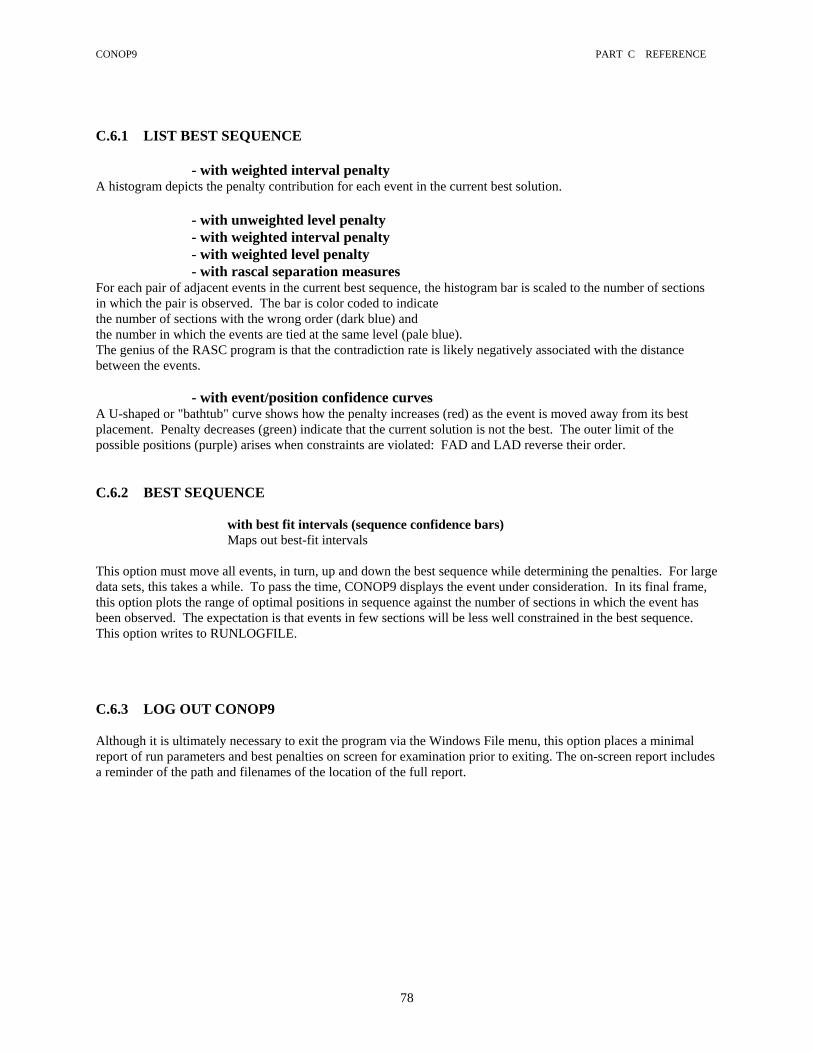
CONOP9 PART C REFERENCE

78

C.6.1 LIST BEST SEQUENCE

- with weighted interval penalty

A histogram depicts the penalty contribution for each event in the current best solution. - with unweighted level penalty - with weighted interval penalty - with weighted level penalty - with rascal separation measures

For each pair of adjacent events in the current best sequence, the histogram bar is scaled to the number of sections in which the pair is observed. The bar is color coded to indicate the number of sections with the wrong order (dark blue) and the number in which the events are tied at the same level (pale blue). The genius of the RASC program is that the contradiction rate is likely negatively associated with the distance between the events.

- with event/position confidence curves A U-shaped or "bathtub" curve shows how the penalty increases (red) as the event is moved away from its best placement. Penalty decreases (green) indicate that the current solution is not the best. The outer limit of the possible positions (purple) arises when constraints are violated: FAD and LAD reverse their order. C.6.2 BEST SEQUENCE

with best fit intervals (sequence confidence bars) Maps out best-fit intervals

This option must move all events, in turn, up and down the best sequence while determining the penalties. For large data sets, this takes a while. To pass the time, CONOP9 displays the event under consideration. In its final frame, this option plots the range of optimal positions in sequence against the number of sections in which the event has been observed. The expectation is that events in few sections will be less well constrained in the best sequence. This option writes to RUNLOGFILE. C.6.3 LOG OUT CONOP9 Although it is ultimately necessary to exit the program via the Windows File menu, this option places a minimal report of run parameters and best penalties on screen for examination prior to exiting. The on-screen report includes a reminder of the path and filenames of the location of the full report.

CONOP9 PART C REFERENCE

79

NAVIGATION KEYS FOR LISTS: PgUp, PgDn, UpArrow, DnArrow -- scroll up and down the list Home, End -- move the bar graph relative to the list of event names [ # ] -- stretch/shrink the bar scale < - + > -- move the red colored name in the list (it helps track positions in the

highly reduced graphs) * / -- zoom in and out % -- return to default settings

CONOP9 PART C REFERENCE

80

C.7 CONOP9 “GRAPHICAL OUTPUT” MENU

Figure: Graphical Output Menu, version 7.3

Starting with version 4.0 (Feb. 2000), the list options at the top of this menu were moved to a separate menu bar (see above). Output options may be viewed repeatedly and revisited until the LOGOFF option is selected. Then the necessary arrays of data are lost!! To re-enter the graphical output menu after logoff, execute a trivially short run with STARTYPE="FILE." STEPS and TRIALS should be set to 1; FORCECOEX should be set to "FILE." Prior to version 5, some of these options started with a message box concerning navigation. Now the same information is a menu option that may be called when needed and does not intrude elsewhere. The traditional navigation keys are reserved by the operating system for manipulating windows on the screen. Therefore CONOP must use other keys -- math signs, brackets, and parentheses. Typically, 'plus' and 'minus' keys move through the events. In some cases the 'x' and 'y' keys direct the next key stroke to the chosen axis, usually this changes the stratigraphic section plotted on that axis. 'Multiply' and 'divide' keys change the scale of the whole graph. The

CONOP9 PART C REFERENCE

81

divide key (/) reduces the font size and fits more of the graphic on the screen. Square brackets alter the maximum value on the y-axis. Curved parentheses shift the image left and right. NOT ALL NAVIGATION KEYS ARE ACTIVE FOR ALL GRAPHS. A NOTE ON GRAPHICS FONTS CONOP3, the DOS implementation of this program, explicitly identified a font file with the parameter GRAPHFONT. Typically it was modern.fon, supplied with the Microsoft FORTRAN Power Station for Windows 3.1. This font has been eliminated from the Windows95 version in favor of automatic selection of the Times New Roman font or any other font file that has been stipulated by Windows setup to substitute when handle "Roman" is called. The program includes the "b," or best, setting which allows the run to find the font that most closely matches the required type face. The basic assumption is that any realistic Windows setup will include numerous fonts and will have set up a substitute for Roman if necessary during normal word-processing operations.

Figure: Graphical Output Menu, version 7.40

CONOP9 PART C REFERENCE

82

C.7.1 RELAXED-FIT CURVES formerly EVENT POSITION CURVES

Plots a graph, for every event, to show the best-known fit as a function of the position of that event in the whole the sequence. In other words, the event would be fixed in a position in the sequence of events, and all others events allowed to move to find the minimum misfit; this would be repeated for all events and positions. Actually, this search is not undertaken systematically, but is reported from the aggregate of all sequences attempted during annealing or tempering. The quality of these curves is quite low if the data set has not been run many times - the event position curves are a

composite of all runs. This means that the reported misfit may be too high, especially for positions that are far from the optimum. Nevertheless, they offer some guidance, because we may often assume that the misfit increases monotonically in both directions away from the optimum. In other words, the curves should have "bathtub" shape without any waves. If waves are present, either too few trials have been run (and all values should be lowered to the minimum value found farther beyond the floor of the tub, on the same side) or there are local minima in the landscape that impact the event position curves. Highly contradictory data sets seem to generate waves I n the event position curves that no amount of re-running can erase. The curves can be deliberately developed by long runs with lots of tempering cycles and a high starting temperature. Selected events can be held close to their initial positions to evaluate seriously non-optimal sequences. The 'EVT', 'LAG', ‘FAR’, ‘END’ and 'FIX' options under SHOWMOVIES allow the run-time graphics to display the progress of the event-position curves. The 'RPT' and ‘BAR’ options for PAUSES allows many runs to be strung together without interruption for user input.

0 200100Arenig

300 400 500 600 700 800Tremad. Lanv. - Lland. Caradoc Ashgill Llandovery Wenlock Ludlow Pri. - Loch.

Proclimacograptus angustatus - LAD (in 6 sections)

MISF

IT

MISFIT RELATIVE TO OPTIMAL SEQUENCES

POSITION IN SEQUENCE OF EVENTS

0.5%

1.0%

0.0%

This drawing is based upon a bitmap saved from a Relaxed-Fit (or Event-Position) Curve.

CONOP9 PART C REFERENCE

83

The raw event-position data are plotted as open red boxes. Filled boxes indicate the best fit solution. Red dots suggest how waves in the plot might be smoothed -- boxes above these dots MAY be the result of too few runs. Green dots are plotted for the secondary misfit measure, if one is active. Where both primary and secondary misfit measures are minimized, the boxes are larger and deep red/brown.

A pale gray background curve plots the number of events that can occupy a given position in the sequence and still achieve the best-known penalty. The value for the mode of this gray curve is plotted in pale gray near the top of the y-axis (look hard in bad light!).

0 200100Arenig

300 400 500 600 700 800Tremadoc Lanv. Lland. Caradoc Ashgill Llandovery Wenlock Ludlow Pri. Loc.

GRAPTOLITEDIVERSITY Basinal Facies only.

Species known from two or more localities.

116 localities425 species

This drawing was prepared from a Relaxed-Fit (or Event-Position) bitmap. It was edited down to the magenta curve in the background of the plot.

SIZE OF UNRESOLVED CLUSTERS OF FIRST- AND LAST-APPEARANCE EVENTS

0 200100Arenig

300 400 500 600 700 800Tremadoc Lanv. Lland. Caradoc Ashgill Llandovery Wenlock Ludlow Pri. Loc.

This drawing was traced from the grey curve on the bitmap saved from the Relaxed-Fit (or Event-Position) curve.

CONOP9 PART C REFERENCE

84

A pale magenta curve shows the running total of FADs minus the LADs. It must climb form zero at the old end of the sequence and fall back to zero at the end. There is no way to avoid an excess of FADs at the old end of a sequence and a surplus of LADs at the young end. This is an artifact of truncating a continuous history of FADs and LADs. The part of the magenta that has a better balance of FADs and LADs will be the most reliable portion of the solution. The least reliable parts of the solution are characterized by high plateaus in the gray curve and persistent steep gradients in the magenta curve. In its final frame, this option plots the range of optimal positions in sequence against the number of sections in which the event has been observed. The expectation is that events in few sections will be less well constrained in the best sequence. This option writes to RUNLOGFILE. C.7.2 BEST-FIT INTERVALS

formerly EVENT-CONFIDENCE BARS A plot of the full range of positions that an event may occupy in sequences that have the optimal fit to the data. Each event is plotted as a bar parallel to the best-fit sequence along the X-axis. The bars indicate the best fit interval as a deep red-brown segment. Extending beyond this is a pale red bar indicative of the relaxed fits better than a threshold value written at the top of the graph. The threshold value may be adjusted with the navigation keys. The threshold is reported in two formats: a % increase in the total misfit above the best-known value; and the same increase expressed as a multiple of the average misfit for a single event. The % measure is not comparable across data sets of different size; the average event misfit normalizes the measure and removes the size effect C.7.3 EVENT CULLING CIRCLES A plot of the full range of positions that an event may occupy in sequences that have the optimal fit to the data. Each event is plotted as a circle whose diameter spans the range of optimal positions. The circles are arrayed in sequence along the X-axis. Use * and / keys to alter the circle sizes. Enlargement causes the x-axis to extend off-screen to the right. Use ] and [ keys to pan left and right across whole diagram when zoomed in. Three versions of this graph follow in succession. They allow different kinds of culling with the ) and ( keys. The first two graphs plot all events and their circles overlap profusely. They may be culled according to the number of sections in which an event has been OBSERVED away from the section ends, or PLACED away from the section ends. The third graph selects the largest set of non-overlapping circles -- the best sub-set of non-contradictory biostratigraphic events. It may be redrafted after culling for a minimum number of sections in which the event is found. The culling algorithm starts at the oldest end of the train of overlapping circles. It takes the first circle and, because this may be a very large circle, it looks inside and will replace it with the contained circle, if any, that has the youngest upper edge. At the upper edge of this circle, it seeks the next entirely younger, non-overlapping circle and looks inside to see if a smaller circle is preferable. This process of taking the next contiguous circle or a smaller one inside it, continues to the top of the section. The culling criteria simply causes the search to skip any circle that is found wanting.

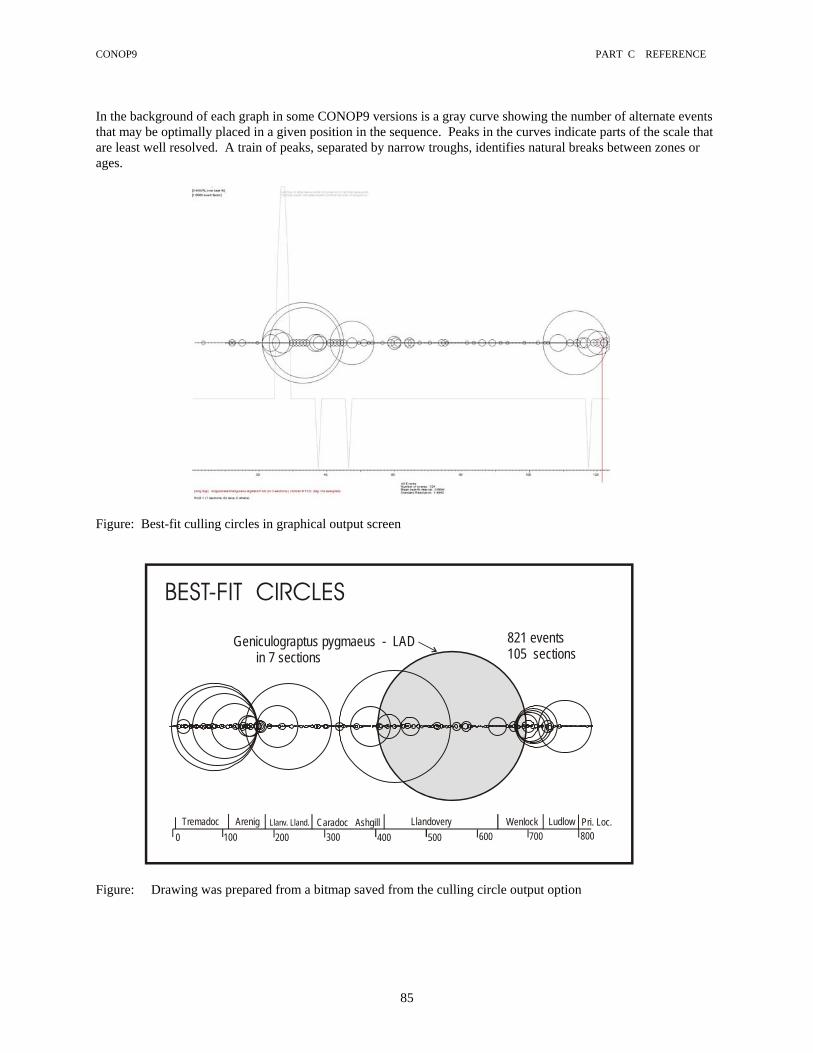
CONOP9 PART C REFERENCE

85

In the background of each graph in some CONOP9 versions is a gray curve showing the number of alternate events that may be optimally placed in a given position in the sequence. Peaks in the curves indicate parts of the scale that are least well resolved. A train of peaks, separated by narrow troughs, identifies natural breaks between zones or ages.

Figure: Best-fit culling circles in graphical output screen

0 200100Arenig

300 400 500 600 700 800Tremadoc Llanv. Lland. Caradoc Ashgill Llandovery Wenlock Ludlow Pri. Loc.

Geniculograptus pygmaeus - LAD in 7 sections

BEST-FIT CIRCLES

821 events105 sections

Figure: Drawing was prepared from a bitmap saved from the culling circle output option

CONOP9 PART C REFERENCE

86

C.7.4 TAXON DURATIONS Histograms and/or cumulative frequency curves of the lengths of taxon ranges AFTER correction for the best fit sequence. In other words, these are not the observed stratigraphic durations that CONTROL9 might read from the input files. The durations are measured in terms of numbers of events in the output sequences. Draws two graphs. The first is a histogram of the frequency distribution of taxon ranges, as measured by levels in the best sequence (i.e. the ordinal composite section). The second is a scatter plot of taxon duration against the number of sections in which a taxon occurs. It scatter plot may be used to investigate claims that the ranges of fossil taxa are determined by the ease with which they may be found. In other words, a long range is a well preserved range and is promoted by the geographically spread of a taxon and its abundance. For short ranges the worry is more serious: they may represent a short-lived taxon or a rare taxon that is under-represented in collections. Of course, the plots cannot dispel the worries. C.7.5 RANGE EXTENSIONS Histograms and/or cumulative frequency curves of the lengths of taxon range extensions AFTER correction for the best fit sequence. In other words, these are the additions to the observed stratigraphic ranges. C.7.6 TAXON DIVERSITY Taxon diversity plotted as a running total of originations minus extinctions against the best sequence on the X-axis. Cycle through the various composite sequences using the x-key followed by plus or minus keys. Draws two graphs of taxon diversity against the full range of composite sections. Diversity is calculated for every event: i.e. every level in the composite. The first graph is a straightforward running total of range ends in which FADs count plus one and LADs minus one. It is standing diversity, as preserved by the input data. The time scale for the diversity curve is provided by the composite sections. Change the composite section scale by using the ‘+’ and ‘-‘ keys. If the input includes tags for events and sections, use the ‘]’ and ‘[‘ keys to walk backward and forward through a set of embedded curves that depict one classification at a time. The first options are for single event tags. The final options are based upon sections. Note that each event can have only one event tag but may qualify for more than one section tag because events may occur in more than one section. The filter does not look for events that are exclusive to one section type; it uses all events found with each section type. As a result, the individual curves for event tags will add up to the overall curve. The individual curves for section tags will not “stack,” they must be expected to add up to more than the overall curve. The second graph plots diversity per section. That is, the diversity is divided by the number of sections that span the given level. It permits examination of the worry that peaks in diversity reflect peaks in collecting. The result is not easily related to standing diversity; and the “correction factor” does not deal effectively with critical differences between sections. Sections are not equally fossiliferous; sections are not all collected with the same intensity; and sections may or may not preserve the same sedimentary facies and the same faunal provinces. - stacked best-fit curves The diversity curve is no more unique than the best-fit solution. Ideally the diversity curve should be a band that includes all curves resulting from the whole set of equally-well-fit solutions. It might also be extended to include all the curves generated by nearly-best-fit sequences. This graphic attempts to map out the confidence band. It uses the conservative search procedure – “hold the sequence while moving one event at a time.” A more complete map requires the much more time consuming strategy – “hold each event at each position in turn, while allowing the rest of the sequence to re-optimize.” To approach this completeness for the diversity curve, many stacked curve graphics must be superimposed by saving the screens as bit maps and combining them in an illustrator program.

CONOP9 PART C REFERENCE

87

The best-fit solution is held fixed as each event in turn is moved up and down the sequence. This is the same as the list-output-menu option to map out the best-fit intervals, except that the diversity curve is on the screen. Whenever a permutation is found that is “close enough” to the best solution, the diversity curve is redrawn. All curves remain superimposed to generate a diversity band that acts as a reliability interval encasing all possible best-fit curves. “Near enough” is determined by the NEARENOUGH parameter in the CFG file. When NEARENOUGH=0.0, the best fit must be matched exactly or improved. If NEARENOUGH=1.0, then any sequence is accepted that has a misfit equal to, or better than, the best known fit plus one average range extension. The average range extension is determined by dividing the best fit by the number of locally observed ranges. In other words, the margin between the best fit and a significantly worse fit is given by: (BEST-FIT x NEARENOUGH-VALUE) / number of locally observed ranges The diversity curves are scaled according to the composite section selected by COMPOSTYPE in the CFG file. The ‘+’ and ‘-‘ keys are disabled. While the stack is being drawn, most operating systems fail to allow keyboard interaction! If the data set is very large, this graphic may tie up all the computer resources for hours. This graphic output option first plots a simple diversity curve and then waits for user input. Strike the enter key. It then considers each event from youngest to oldest in the best-fit sequence. The progress through these events is charted by a line that grows parallel to the base-line from right to left. The line is erased when the plot is complete. In the bottom left corner there is a counter that reports all the misfit values. Remember that the diversity curve is scaled so that the modal value touches the top of the screen. If this peak is reduced, the whole curve shifts up. - section correction Taxon diversity might be influenced by the number of sections that span different parts of the curve -- more sections mean a chance to collect more fossils and taxa, especially is they represent a wide range of facies. Draws two graphs that may influence the interpretation of the diversity plots. The first is shows the number of sections in which the event at each level has been observed. Typically this plot will be as wild and noisy set of sawtooths. If, however, parts of the sequence are characterized by a cluster of relatively or low values, then there is evidence that preservation, or collection, or provinciality varies systematically with position in the sequence. The diversity curves might be correspondingly biased. The second graph shows the number of sections that span each level. It counts all the sections in which the given event has been placed away from the end. The inference is that the section should span the corresponding time interval, whether or not the event is recorded there. These are the values used to “adjust” the taxon diversity for the second graph in that category. C.7.7 MEAN EXTANT TAXON LONGEVITY A plot of the average duration of all taxa that range through each position in the best sequence. The plot cycles through all the composite sequences, forward and backward by means of the ‘+’ and ‘-‘ keys (Shift key not needed). For the ORDINAL composite, longevity is measured in terms of the number of biological origination and extinction events that occur during the taxon range. For all other composites, the longevity is estimated from relative stratigraphic thicknesses. Limited data suggest that the best proxy for a time scale is provided by the “ZERO MEAN STANDARD” composite. Two cycles of plots are presented. The second always begins after the user exits the first using the Esc key. The first cycle plots mean longevity against time. The second cycle plots longevity against standing diversity. The latter plots typically show two trends. In the long tern trend, longevity and diversity rise and then fall together. The long-term curve tends to be concave up; i.e. diversity increases faster. The long term trend reflects the end effects

CONOP9 PART C REFERENCE

88

of sampling intervals or whole clades. The short term fluctuations run at right angles to the long term trend. They describe the major extinctions and diversifications; in these, diversity and longevity are strongly negatively correlated. Minima in diversity curves are characterized by the longer-lived taxa only. High diversity is achieved by adding relatively short-lived taxa. Two some extent, this is an unremarkable result of a wide range in longevity -- if taxa and extinctions are placed at random, long-lived taxa are more likely to span extinctions. In other words, extinctions that targeted long-lived taxa would tend to limit the length of taxon ranges. If some taxa can be longer lived than the waiting time between diversity crises, they must be the survivors. C.7.8 PACE OF ORIGINATION/EXTINCTION Two plots that attempt to extract the rate of origination and extinction, without including time “bins.” Thus, they seek to exploit the event-based sequence and avoid zonal artifacts. Origination rate is related to the interval between successive originations. The plots use these intervals; hence, the term “pace” not rate. At each event in sequence, the interval is measured forward and backward to the nearest originations (or extinctions). Thus all events generate a value for the current pace. The noise is reduced by applying a three-interval moving average. Finally, the time series of 3-interval averages is plotted upside-down. That is, the smallest interval (often zero) is plotted at the top of the screen and the largest value is plotted at the bottom. Thus, the time series rises and falls as the rate increases and decreases. A suite of time series is plotted using the whole array of composite sections. For the ordinal composite, pace is measured in terms of the number of intervening events. For all other composites, the pace is measured in terms of the composite stratigraphic thickness. A second plot for originations and extinctions uses runs of consecutive like events. It is another attempt to retain the interval-free character of the best-fit sequence. Although runs are a form of bin, at least the bin size is determined by and varies with the data. Both the plots of runs and pace are typically very noisy; that is the price of retaining minimal intervals. C.7.9 PAIRWISE CONTRADICTIONS A plot of the frequency of observed pairwise sequences that contradict the final sequence -- as a function of the distance between the events in the final sequence. The fraction of contradictory observations should fall systematically as the separation increases. What does it mean if the contradiction rate is still high at large separations? The final sequence may be far from optimal, as in a short run; or the taxa may be rather long-lived relative to the time span of the sections. Usually, the adjacent pairs of events in the best sequence contradict 20-30% of the local observations. For a highly contradictory data set, there may be two modes. Remember that there will be many pairs with short separation, but only one pair has the maximum separation (number of events minus one). So the sample size and confidence level fall systematically as the separation increases. Tiny dots on the graph plot the contradictions for individual pairs of events.

- by separation - by mean range length - by coexistence

After version 3.3, this option walks through 9 different graphs. Starting with version 4.0 the 9 graphs drawn by this menu item were separated into 3 menu items. This is desirable for large instances of the data set for which the graphs draw themselves rather slowly. The nine graphs are as follows. The contradiction rate can be plotted against the separation of events (graphs 1-3) or against the average length of the two associated ranges (graphs 4-9). The range lengths may be considered for all

CONOP9 PART C REFERENCE

89

pairs of taxa (graphs 4-6) or only for pairs of taxa that actually overlap in the composite sequence (graphs 7-9). In each of the graph triplets, one includes all event types (graphs 1, 4, 7), only FAD-FAD event pairs (graphs 2, 5, 8), or only LAD-LAD event pairs (3, 6, 9). This subdivision has theoretical and practical purposes. It can test academic theories about range ends and it can handle data sets in which either FADs or LADs are corrupted (caving and reworking problems).

Figure: CONOP graphical output of contradition rate as a function of separation of pairs of events

CONOP9 PART C REFERENCE

90

Figure: CONOP graphical output of contradiction rate as function of length of ranges of event pairs

Figure: CONOP graphical output of contradictions as function of range duration but limited to pairs of events for

coexisting pairs of taxa

CONOP9 PART C REFERENCE

91

PAIRWISE CONTRADICTIONS BETWEENLOCALLY OBSERVED SEQUENCES

Figure: Diagram traced from a bitmap saved from the Pairwise Contradiction screen.

If two taxa do not have overlapping ranges, there events cannot be preserved out of order simply because of the underestimation of ranges. Longer ranged taxa tend to overlap with more others than short-ranged taxa. These two influences must be teased apart in any analysis of contradictions. For this reason a range of nine graphs is provided even though it will seem excessive or redundant to the casual observer. C.7.10 THE TAXON RANGE CHARTS These traditional range charts are 1-dimensional views of the multidimensional solutions. The range charts are presented section by section. The chart shows observed ranges (black), range extensions (red), and placement of un-observed ranges/events (pink). Other colors treat more exotic possibilities that arise as errors or when range contractions are permitted. Walk through the different sections and the composite sections on the x-axis by typing ‘x’ followed by ‘+’ or ‘-’. But in to the time in Version DEC 7.31 introduced three different options for the sequence of taxon ranges in the chart: input file order (taxon 1 at top); FAD order (earliest first appearance at top); and LAD order (latest last appearance at top). [this option was activated by the ONE-BY-ONE parameter in CONOP3.CFG]

CONOP9 PART C REFERENCE

92

Figure: Composite range increments (red), composite range (black), and composite range support (pink histogram).

This graphic option was added with version 7.40. The pink histogram was added with version 7.43. To change the x-axis composite scaling, type {X}, followed by {+} or {-}. To cycle through other taxa with same x-axis scale, type {+} or {-}.

C.7.11 COMPOSITE RANGE INCREMENTS Starting with version 7.40, this option plots local observed ranges, in red, against the composite range, in black. Black and red ranges have small squares at their ends; if the local range extends to the top or base of the measured section, the corresponding square is omitted. Vertical grey lines mark limits of composite range. Plotted ranges are two pixels longer than actual ranges; this enables single-horizon ranges to be recognized. If there are fewer than 50 sections, the local sections always plot on the same screen row. If there are more than 50 sections, the empty spaces (sections that do not include taxon) are closed up. The local section levels are mapped into the composite sequence using the line of clorrelation (LOC; red line in 2-D charts). Because the LOC is a result of the sequencing process, the position of the observed ranges (red lines) is a property of the solution, NOT independently determined. The primary purpose of the graphic is to identify which sections determine the limits of the composite range. It has the potential to highlight anomalous taxonomy, reworking, or insufficient sampling.

Use {+} and {-} keys to walk through the taxon ranges and other events. Use {X} key followed by {+} or {-} keys to walk through different composite scaling options.

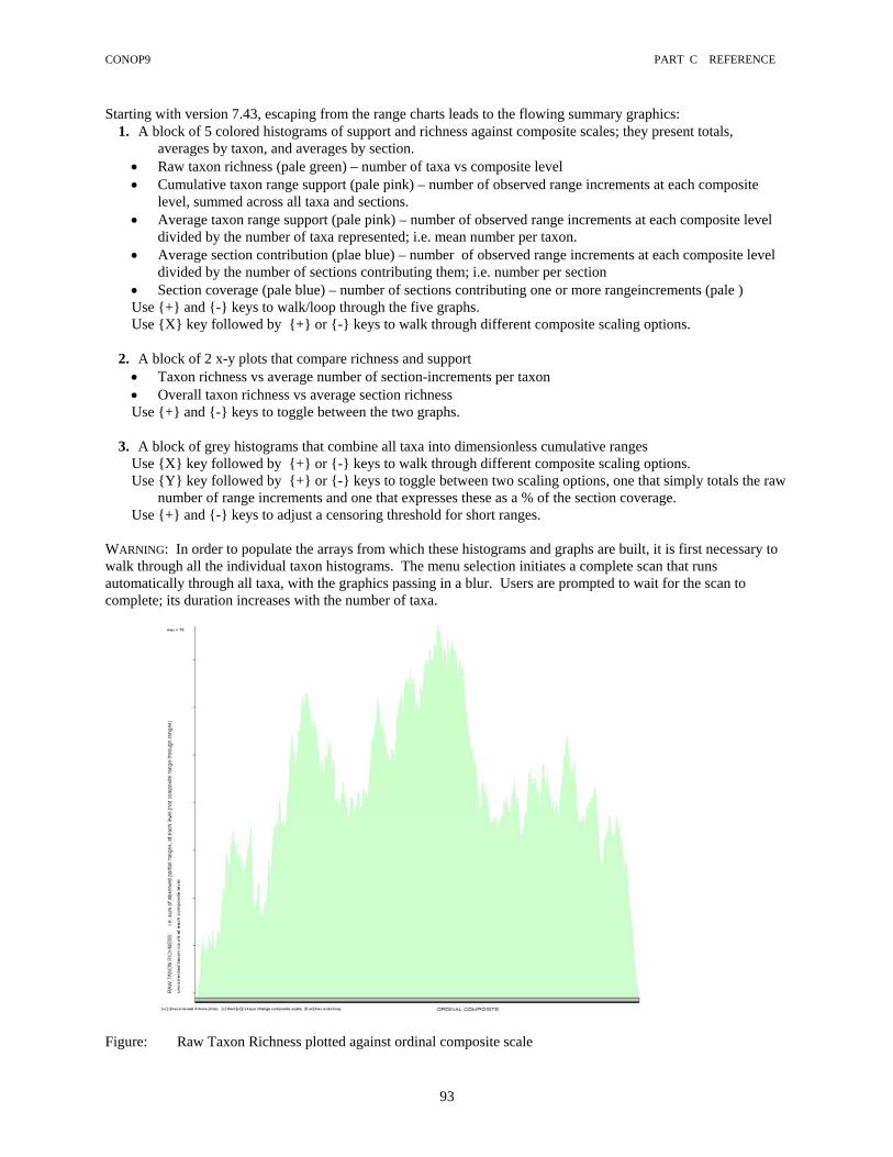
CONOP9 PART C REFERENCE

93

Starting with version 7.43, escaping from the range charts leads to the flowing summary graphics: 1. A block of 5 colored histograms of support and richness against composite scales; they present totals,

averages by taxon, and averages by section. • Raw taxon richness (pale green) – number of taxa vs composite level • Cumulative taxon range support (pale pink) – number of observed range increments at each composite

level, summed across all taxa and sections. • Average taxon range support (pale pink) – number of observed range increments at each composite level

divided by the number of taxa represented; i.e. mean number per taxon. • Average section contribution (plae blue) – number of observed range increments at each composite level

divided by the number of sections contributing them; i.e. number per section • Section coverage (pale blue) – number of sections contributing one or more rangeincrements (pale ) Use {+} and {-} keys to walk/loop through the five graphs. Use {X} key followed by {+} or {-} keys to walk through different composite scaling options.

2. A block of 2 x-y plots that compare richness and support • Taxon richness vs average number of section-increments per taxon • Overall taxon richness vs average section richness Use {+} and {-} keys to toggle between the two graphs.

3. A block of grey histograms that combine all taxa into dimensionless cumulative ranges

Use {X} key followed by {+} or {-} keys to walk through different composite scaling options. Use {Y} key followed by {+} or {-} keys to toggle between two scaling options, one that simply totals the raw

number of range increments and one that expresses these as a % of the section coverage. Use {+} and {-} keys to adjust a censoring threshold for short ranges.

WARNING: In order to populate the arrays from which these histograms and graphs are built, it is first necessary to walk through all the individual taxon histograms. The menu selection initiates a complete scan that runs automatically through all taxa, with the graphics passing in a blur. Users are prompted to wait for the scan to complete; its duration increases with the number of taxa.

Figure: Raw Taxon Richness plotted against ordinal composite scale

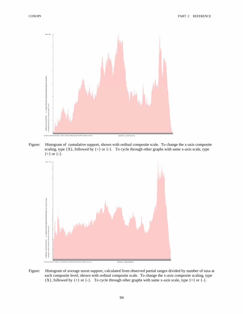
CONOP9 PART C REFERENCE

94

Figure: Histogram of cumulative support, shown with ordinal composite scale. To change the x-axis composite

scaling, type {X}, followed by {+} or {-}. To cycle through other graphs with same x-axis scale, type {+} or {-}.

Figure: Histogram of average taxon support, calculated from observed partial ranges divided by number of taxa at

each composite level, shown with ordinal composite scale. To change the x-axis composite scaling, type {X}, followed by {+} or {-}. To cycle through other graphs with same x-axis scale, type {+} or {-}.

CONOP9 PART C REFERENCE

95

Figure: Histogram of average section contribution; i.e. average number of supporting observed ranges, for each

position in composite, divided by number of sections at that position. To change the x-axis composite scaling, type {X}, followed by {+} or {-}. To cycle through other graphs with same x-axis scale, type {+} or {-}.

Figure: Histogram of section coverage; i.e. number of sections contributing at least one range increment per

composite level. To change the x-axis composite scaling, type {X}, followed by {+} or {-}. To cycle through other graphs with same x-axis scale, type {+} or {-}.

CONOP9 PART C REFERENCE

96

Figure: Example plot of taxon richness against average support per taxon. To toggle between two graphs with

same y-axis, type {+} or {-}.

Figure: Example of plot of taxon richness against average taxon richness per section. Because the per-section richness must be equal to or lower than the sum of section richnesses, points cannot fall beow the y=x line scribed on the graph (unless due to Fortran rounding errors). To toggle between two graphs with same y-axis, type {+} or {-}.

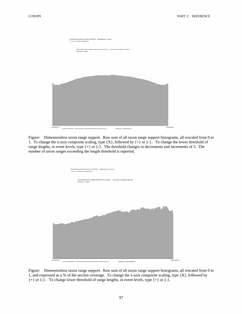
CONOP9 PART C REFERENCE

97

Figure: Dimensionless taxon range support. Raw sum of all taxon range support histograms, all rescaled from 0 to 1. To change the x-axis composite scaling, type {X}, followed by {+} or {-}. To change the lower threshold of range lengths, in event levels, type {+} or {-}. The threshold changes in decrements and increments of 5. The number of taxon ranges exceeding the length threshold is reported.

Figure: Dimensionless taxon range support. Raw sum of all taxon range support histograms, all rescaled from 0 to 1, and expressed as a % of the section coverage. To change the x-axis composite scaling, type {X}, followed by {+} or {-}. To change lower threshold of range lengths, in event levels, type {+} or {-}.

CONOP9 PART C REFERENCE

98

C.7.12 COLLECTION QUALITY Presents plots of the distribution of observed events and taxa, level by level. These logs allow the evaluation of the quality of each collection level in terms of abundance and fidelity of information. Events are plotted to the left. A gray bar records the number of events observed at that level. The light green portion is the number observed at the correct level, according to the solution. Taxa are plotted to the right. The gray bar records the number that are correctly observed as range ends or within the expected range according to the solution. The dark red portion of the bar records the number of taxa that were "missing" in the sense that the solution drew a range extension through that level. Only taxa that were observed somewhere else in the section are included in the dark green bar; i.e. light green is a sign of high quality ; dark red is a sign of failure to collect [this option was activated by the ONE-BY-ONE parameter in CONOP3.CFG]

C.7.13 2-SECTION LOCS Plots traditional 2-dimensional Lines of Correlation after run. These are 2-dimensional projections of the full solution, which has a dimension for every section. Therefore, the LOC can be influenced by sections other than the two on the plot; and may include steps and gradient changes that cannot be understood solely in terms of the shared events. The raw line of correlation shown in solid red and a 3-point smoothed LOC is shown in dashed pink. The coordinates of events observed in both sections are shown in green. FADs and LADs are plotted as right-angle symbols that should be understood as the corners of an error box. Observed FADs may be moved down-section only; the open ends of the symbol point in these directions. If the event has zero weight in one of both sections, the corresponding arms of the symbol are reduced to half length. Unpaired events, which may not move up or down section when drawing the LOC are plotted as boxes. The x-axis runs through all sections in turn, and then the seven options for the composite section. The y-axis cycles through all local sections and the composite sections, too. Thus any pair of sections and/or composites may be compared. In some versions of the program, a final option for the y-axis plotted all the local sections together if one of the composite sections appeared on the x-axis. This "all sections" option tended to become unstable; it is not supported in the latest versions. Type ‘x’ or ‘y’ followed by ‘+’ or ‘-’ to change sections on the corresponding axis. Use ‘>’ or ‘<’ to go to the last or first section. Use ‘Shift +’ or ‘Shift -’ to skip up or down the section dictionary order five sections at a time.

CONOP9 PART C REFERENCE

99

Figure: 2-D Line of Correlation; example shows a single section plotted against a composite. All event levels are shown as short black ticks outside the section bars. Starting with version 7.42, those event levels represented in the other section are drawn into the grey bars as darker grey lines. Thus the x-axis section is shown as a projection into the y-axis section and vice versa. If one of the sections is a composite section, the projection of the other is shown by red lines. The green right-angle symbols are the coordinates of shared taxon range ends; they are oriented like arrow heads pointing into the taxon range, thus differentiating first- and last-occurrence ends of the range and allowing the symbols to be regarded as corners of an uncertainty box on the possible true coordinates; range-events are projected into the LOC parallel to an open end of the angle symbol (only one of these points toward the LOC). When one axis is an optimal composite section, the LOC must follow a path between the first- and last-occurrence symbols, because the composite ranges are not subject to exension.

CONOP9 PART C REFERENCE

100

Figure: 2-section LOC for CONOP composite section against a zonal composite. After version 7.42, the non-CONOP composite section is projected into the CONOP composite as red event-horixons, as shown here.

Date

d Tu

ffs w

ith B

iost

ratig

raph

ic Co

ntro

l

“Z-standard” Composite Shale Section

Myr b.p.

Figure: Drawing based upon a Two-Dimensional LOC screen that plotted one section containing

radioisotopically dated beds against a composite section. The saved bitmap had a piecewise linear LOC; it was smoothed by the drawing program.

CONOP9 PART C REFERENCE

101

If the composite sections (other than ordinal) do not plot any event levels or LOC (except perhaps at edge of screen), check the section dictionary. It may be that none of the sections is marked for inclusion in the compositing process. If the CURVFILE is active, and the current best penalty is equal to the best known (minimum value in CURVFILE), two sets of graphs will be presented. The second set of the graphs include pink boxes error/confidence boxes that represent the full range of equally good fits -- the flat bases of the event-position-curves. For the composite sections, the box is based upon the range of optimal positions in sequence. For the real sections, the box is based upon the solutions to locating task, for all solutions with the best known fit. As more and more boxes overlap, the pink is darkened through red and into purples. The limit is about 20 sections. Acceptable LOCs must pass through all boxes; so, darker colors mark the preferred track for LOCs. The boxes are drawn relatively slowly, because it is necessary to check colors pixel by pixel. When the window is maximized, the boxes can be observed to fill; when the window is small and the filling process cannot be seen, the program appears to have hung. The boxes may also be meaninglessly large if the current best-fit is not optimal; they flood the window; so the option is automatically switched off for searches that end in a sub-optimal solution. The regular red LOC and green event coordinates are superimposed on the pink boxes. But the smoothed LOC (dashed) is omitted. The size and reliability of the pink boxes will likely vary with the number of equally well-fit solutions that are tried. Many such solutions are likely to have been fit to the data if the search runs beyond the first find of the best penalty. This set of equally-well-fit solutions can be searched deliberately by starting from a "file" with one of the best solutions and then making a very large number of conservative changes (small neighborhood; low temperature). [this option was activated by the TWO_BY_TWO parameter in CONOP3.CFG] C.7.14 FENCE CHARTS

- with 3-pt smoothing - with 5-pt smoothing - with 7-pt smoothing

Draws fence diagrams to illustrate the solutions after the run. There are four options with different degrees of smoothing. The raw solution locates all events at a collecting horizon. The smoothing separates these "ties." The sections are scaled according to their relative thickness. The vertical scale is adjusted to accommodate the thickest local section above the baseline and the thickest local section below the baseline. Consequently, the scale may be forced to change if the baseline changes. The base line for the plots is one event. Its tie-line is plotted in red, but turns black where it coincides with other events. Navigation keys allow the base-line event to be moved up and down the sections. The image repaints each time and re-scales the sections if necessary. About 20 sections may reasonably be plotted on one screen. If more than one screen is needed, then there is a 5 section overlap between screens. [this option was activated by FENCECHART parameter in CONOP3.CFG] C.7.15 SECTION RANGE CHARTS Five charts plot the range of individual sections against the best sequence of events. Section thickness is lost in these charts; they simply show the time span of the section against a time scale that has one equal unit for each event., i.e. an ordinal time scale, running vertically from oldest at the bottom of the screen to youngest at the top. The first chart shows sections as a gray rectangle, in which the collection horizons plot as darker strips. The next four plots use a color-code for the interior of the box to show the distribution of penalty increments by observed event and the stratigraphic resolution. The penalty is the misfit between the observed and the placed event horizon. The resolution is the stratigraphic distance between two adjacent events in the composite section. The solution

CONOP9 PART C REFERENCE

102

always places the events in a unique order without any "ties." But some pairs of events may not be separable in any section when the locating task is completed; logically, these are events whose relative order in the best sequence is actually arbitrary. The penalty increments are shown first in meters, then in levels. The resolution is shown first in local meters then in the standardized units used for the composite. White means no penalty because the event is not observed. Black means no resolution because adjacent events are placed at same level. Red means highest 10 percentile penalty or resolution; blue means lowest 10 percentile penalty or resolution; the color bar plots are shown with arithmetic and logarithmic scales in order to highlight different aspects of the distribution of penalty and resolution values. As many as 256 sections have been plotted on one high-resolution screen. The sections are squeezed progressively as the number increases. The program attempts to plot all sections at first. The number of sections may be adjusted interactively. If more than one screen is needed, then there is a 5 section overlap between screens. The width of the section columns depends upon the number of pixels in a horizontal row across the screen. The resolution of events within the columns depends upon the number of pixels in a vertical column down the screen. In large data sets this screen resolution may be radically exceeded by the number of events. In this situation, some events may scale to spaces between the rows of pixels and disappear; i.e. the scaling algorithm does not lead to a black blur, but drops some bars and thus understates the completeness. Plans to offer an algorithm that produces the black blur (overstated completeness) in response to inadequate screen resolution have not been completed. The necessary data for constructing an algorithm at full resolution can be obtained by setting SECT_OUT=’MIN’. [this option was activated by RANGECHART parameter in CONOP3.CFG] A NOTE ABOUT THE VERTICAL SPAN OF SECTIONS IN THESE PLOTS: CONOP places all the events in every section. Typically, especially in seriation problems, many events are placed at the highest or lowest levels in the section, because their true age is interpreted to lie beyond the span of the section. In its simplest form, the Section Range algorithm might eliminate all events placed at these levels and determine the span of the section solely from events placed at intermediate levels. But, this can underestimate the stratigraphic span of the section because there are two legitimate placements of events at the limits of the section. A first-appearance event observed and placed at the highest level and a last appearance event observed and placed at the lowest level would both be good indicators of events within the span of the section. A last occurrence event should not be lower than its observed level; a first occurrence should not be higher. Consequently, the algorithm must work a little harder and search for events of this type. When they exist, the span of the section is extended to include them.

- full range - truncated

Starting with version DEC 7.0, there are two Section Ranges options in the Graphical Output Menu. The “full-range” option is the stratigraphically correct one, as described above. The “truncated” option does not include any range-end events placed at the highest and lowest levels. The legitimate use of the truncated option is to allow quick comparison with the full plot to determine the importance of the highest and lowest levels. For many instances of the correlation problem, the two graphics will be identical, or nearly so. Instances in which the plots are substantially different will be characterized by the following pattern of field observations: at those range ends which shift dramatically between the two options, there will be one or more taxa found only at the highest or the lowest level. Terminal portions of sections that disappear in the truncated plots are easily overlooked in the fence diagrams and the 2-D Lines of Correlation. In fence diagrams they may generate pale blue lines, but only if they correlate to levels within the neighboring sections. In 2-D section correlations, they correspond to portions of the LOC (red lines) that coincide with the perimeter box of the plot. Such LOC segments can indicate that the very top or bottom of one section correlates with a finite span of the other section. Of course, the same appearance results when part of one section is entirely younger or older than the other. Thus, the truncated section range chart may better match our expectations after examination of the fence diagrams and 2-D plots.

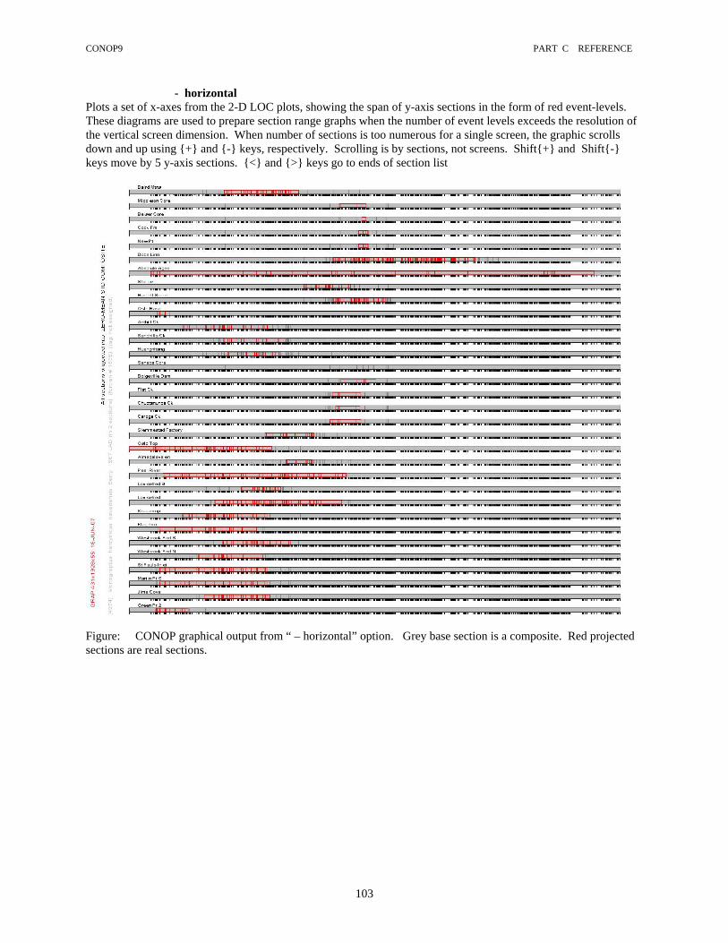
CONOP9 PART C REFERENCE

103

- horizontal Plots a set of x-axes from the 2-D LOC plots, showing the span of y-axis sections in the form of red event-levels. These diagrams are used to prepare section range graphs when the number of event levels exceeds the resolution of the vertical screen dimension. When number of sections is too numerous for a single screen, the graphic scrolls down and up using {+} and {-} keys, respectively. Scrolling is by sections, not screens. Shift{+} and Shift{-} keys move by 5 y-axis sections. {<} and {>} keys go to ends of section list

Figure: CONOP graphical output from “ – horizontal” option. Grey base section is a composite. Red projected sections are real sections.

CONOP9 PART C REFERENCE

104

CONOP9 PART C REFERENCE

105

Figure: Span of graptolite-bearing sections, a diagram prepared in two panes by tracing ‘Section Ranges’

graphical output from CONOP9. Individual section details traced from ‘ – horizontal’ option.

CONOP9 PART C REFERENCE

106

C.7.16 RERUN SEARCH; NO OUTOUT FILE This option appeared in early versions of CONOP9. It was removed for lack of use. Its purpose has been replaced by the "RPT" setting of the PAUSES parameter. C.7.17 LOG OUT CONOP9 Although it is ultimately necessary to exit the program via the Windows File menu, this option places a minimal report of run parameters and best penalties on screen for examination prior to exiting. The on-screen report includes a reminder of the path and filenames of the location of the full report.

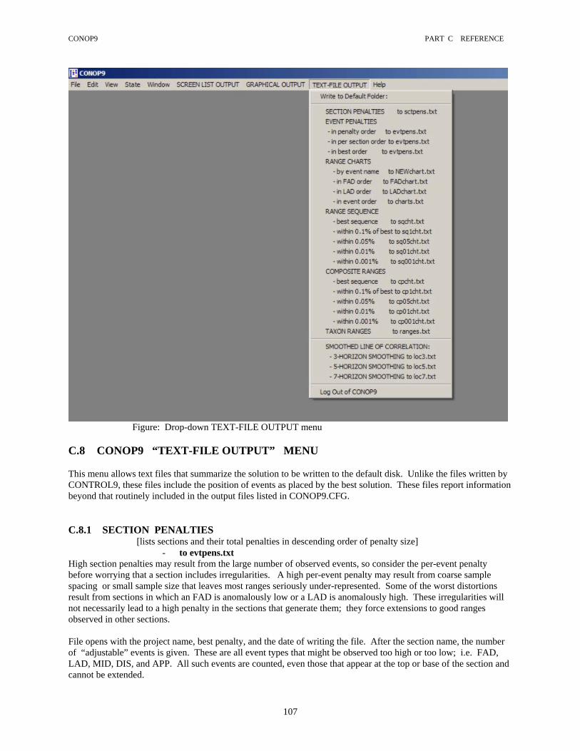
CONOP9 PART C REFERENCE

107

Figure: Drop-down TEXT-FILE OUTPUT menu

C.8 CONOP9 “TEXT-FILE OUTPUT” MENU This menu allows text files that summarize the solution to be written to the default disk. Unlike the files written by CONTROL9, these files include the position of events as placed by the best solution. These files report information beyond that routinely included in the output files listed in CONOP9.CFG. C.8.1 SECTION PENALTIES

[lists sections and their total penalties in descending order of penalty size] - to evtpens.txt

High section penalties may result from the large number of observed events, so consider the per-event penalty before worrying that a section includes irregularities. A high per-event penalty may result from coarse sample spacing or small sample size that leaves most ranges seriously under-represented. Some of the worst distortions result from sections in which an FAD is anomalously low or a LAD is anomalously high. These irregularities will not necessarily lead to a high penalty in the sections that generate them; they force extensions to good ranges observed in other sections. File opens with the project name, best penalty, and the date of writing the file. After the section name, the number of “adjustable” events is given. These are all event types that might be observed too high or too low; i.e. FAD, LAD, MID, DIS, and APP. All such events are counted, even those that appear at the top or base of the section and cannot be extended.

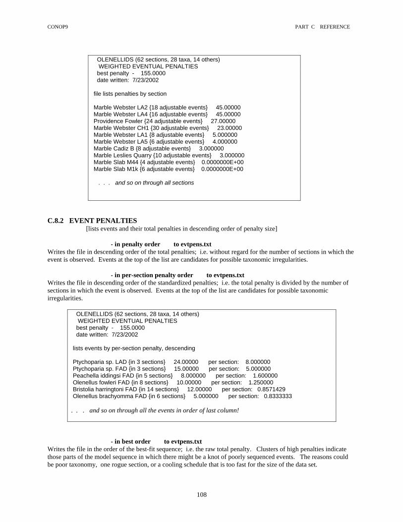
CONOP9 PART C REFERENCE

108

OLENELLIDS (62 sections, 28 taxa, 14 others) WEIGHTED EVENTUAL PENALTIES best penalty - 155.0000 date written: 7/23/2002 file lists penalties by section Marble Webster LA2 {18 adjustable events} 45.00000 Marble Webster LA4 {16 adjustable events} 45.00000 Providence Fowler {24 adjustable events} 27.00000 Marble Webster CH1 {30 adjustable events} 23.00000 Marble Webster LA1 {8 adjustable events} 5.000000 Marble Webster LA5 {6 adjustable events} 4.000000 Marble Cadiz B {8 adjustable events} 3.000000 Marble Leslies Quarry {10 adjustable events} 3.000000 Marble Slab M44 {4 adjustable events} 0.0000000E+00 Marble Slab M1k {6 adjustable events} 0.0000000E+00 . . . and so on through all sections

C.8.2 EVENT PENALTIES [lists events and their total penalties in descending order of penalty size]

- in penalty order to evtpens.txt

Writes the file in descending order of the total penalties; i.e. without regard for the number of sections in which the event is observed. Events at the top of the list are candidates for possible taxonomic irregularities.

- in per-section penalty order to evtpens.txt Writes the file in descending order of the standardized penalties; i.e. the total penalty is divided by the number of sections in which the event is observed. Events at the top of the list are candidates for possible taxonomic irregularities.

OLENELLIDS (62 sections, 28 taxa, 14 others) WEIGHTED EVENTUAL PENALTIES best penalty - 155.0000 date written: 7/23/2002 lists events by per-section penalty, descending Ptychoparia sp. LAD {in 3 sections} 24.00000 per section: 8.000000 Ptychoparia sp. FAD {in 3 sections} 15.00000 per section: 5.000000 Peachella iddingsi FAD {in 5 sections} 8.000000 per section: 1.600000 Olenellus fowleri FAD {in 8 sections} 10.00000 per section: 1.250000 Bristolia harringtoni FAD {in 14 sections} 12.00000 per section: 0.8571429 Olenellus brachyomma FAD {in 6 sections} 5.000000 per section: 0.8333333 . . . and so on through all the events in order of last column!

- in best order to evtpens.txt Writes the file in the order of the best-fit sequence; i.e. the raw total penalty. Clusters of high penalties indicate those parts of the model sequence in which there might be a knot of poorly sequenced events. The reasons could be poor taxonomy, one rogue section, or a cooling schedule that is too fast for the size of the data set.

CONOP9 PART C REFERENCE

109

C.8.3 RANGE CHARTS [writes or overwrites to default folder; does not prompt for name or overwrite]

- in event order to charts.txt - in FAD order to FADchart.txt - in LAD order to LADchart.txt

Write a file with the extended range charts, section by section. Each section has its own sub-heading and is plotted as a list of all taxa placed away from the ends of the section. The file resembles the brief version of sections.txt, as written by CONTROL9, but gives the extended ranges. The following box illustrates the file using the initial part of the output for a run of the Riley data set.

RILEY (7 sections, 62 taxa, 0 others) best penalty - 3546.000 date written: 1/24/2000 file lists range placements for one solution ________________________________________________ ________________________________________________ 1 - Morgan Creek (Mor) __________________________________ Number of Local Event Levels: 25 Number of Locally Observed Events: 92 Mean Number of Events per Level: 3.680 Highest Event Level: 1796.000 Lowest Event Level: 1444.000 Thickness of Collected Interval: 352.000 Mean level spacing: 14.667 Standard Deviation of level spacing: 18.612 ----- Adjusted Ranges (Observed Ranges) FAD: 1796.000 (1796.000) LAD: 1751.000 (1738.000) Dysoristus lochmanae FAD: 1792.000 (not seen) LAD: 1686.000 (1686.000) Labiostria sigmoidalis FAD: 1792.000 (1796.000) LAD: 1707.000 (1694.000) Apsotreta expansus FAD: 1769.000 (not seen) LAD: 1668.000 (1668.000) Dytremacephalus granulosus FAD: 1769.000 (1769.000) LAD: 1754.000 (not seen) Aphelaspis longifrons FAD: 1769.000 (1769.000) LAD: 1641.000 (not seen) Dunderbergia variagranula FAD: 1769.000 (not seen) LAD: 1668.000 (1675.000) Labiostria platifrons . . . and so on through the taxa, then repeat for all sections!

C.8.4 RANGE SEQUENCE [writes or overwrites to default folder; does not prompt for name or overwrite]

- best sequence to seqnchart.txt - within 0.1% of best to sq01chrt.txt - within 1% of best to sq1chrt.txt - within 5% of best to sq5chrt.txt - within 10% of best to sq10chrt.txt

CONOP9 PART C REFERENCE

110

Write files that shows the ranges taxon by taxon in the best sequences and includes the best-fit intervals for each range end as determined from CURVFILE. The file may be imported to a spreadsheet or graphing program to prepare a composite range chart with ordinal event spacing (after first eliminating the header lines!). The following box shows the basic file format. Five options allow relaxation of the best-fit interval to relaxed fit intervals at four fixed intervals.

RILEY (7 sections, 62 taxa, 0 others) best penalty - 2882.000 date written: 2/13/2000 file lists ranges by position in best sequence FAD (actual min max) LAD (actual min max) NAME 1 1 1 3 2 3 Modocia cf.oweni 2 2 3 4 4 4 Bolaspidella wellsvillensis 5 5 5 6 6 6 Bolaspidella burnetensis 7 7 7 11 11 11 Cedarina cordilleras 8 8 8 9 9 9 Modocia cf.centralis 10 10 10 55 54 55 Kormagnostus simplex 12 12 12 13 13 13 Cedarina eurycheilos 14 14 15 16 16 17 Meteoraspis cf.robusta 15 14 15 18 17 18 Syspacheilus cf.camurus 17 16 18 50 50 50 Kinsabia varigata 19 19 21 20 20 24 Apsotreta orifera . . . and so on through all 62 taxa

After version 7.36, the repeated listings for unpaired events were eliminated; the second set of numbers was replaced with dashes and the event types were added to the event name. Prior to version 7.36, MID events were not properly handled in these files. After version 7.38, the file dropped the so-called “actual” positions from the most recent solution. The caused too much confusion: if the last solution is not optimal, the “actual” position might not fall between the maximum and minimum. The last solution can be retrieved from several other output files. C.8.5 COMPOSITE RANGES [writes or overwrites to default folder; does not prompt for name or overwrite]

- best sequence to compchart.txt - within 0.1% of best to cp01chrt.txt - within 1% of best to cp1chrt.txt - within 5% of best to cp5chrt.txt - within 10% of best to cp10chrt.txt

Write a file that repeats the coverage of seqnchrt (above) but plots the placed levels in the composite section (COMPOSTYPE) rather than the ordinal positions. Not properly operational at the time of writing. The file may be imported to a spreadsheet or graphing program to prepare a composite range chart with ordinal event spacing (after first eliminating the header lines!). The file format resembles seqnchrt (above), except that the integer values will be replaced by decimal values. Five options allow relaxation of the best-fit interval to relaxed fit intervals at four fixed intervals.

SEYMOUR (4 sections, 19 taxa, 0 others)

CONOP9 PART C REFERENCE

111

best penalty - 2842.020 date written: 8/01/2000 file lists ranges by position in best sequence FAD (actual min max) LAD (actual min max) NAME 1000.000 1000.000 1000.000 1000.000 1000.000 1000.752 Gunnarites bhavaniforms 1000.000 1000.000 1000.000 1000.752 1000.000 1000.752 Maorites tuberculatus 1015.190 1015.190 1015.190 1073.656 1073.656 1073.656 Diplomoceras lambi 1019.568 1019.568 1019.568 1033.955 1033.955 1033.955 Maorites seymourianus 1020.696 1020.696 1020.696 1037.060 1037.060 1037.060 Kitchinites darwini . . . and so on through all events

After version 7.36, the repeated listings for unpaired events were eliminated; the second set of numbers was replaced with dashes and the event types were added to the event name. Prior to version 7.36, MID events were not properly handled in these files. After version 7.38, the file dropped the so-called “actual” positions from the most recent solution. The caused too much confusion: if the last solution is not optimal, the “actual” position might not fall between the maximum and minimum. The last solution can be retrieved from several other output files. C.8.6 TAXON RANGES [writes or overwrites to default folder; does not prompt for name or overwrite]

- to ranges.txt Write a file that shows the extended ranges taxon by taxon. The subheadings are taxa. Each subsection lists the ranges in all sections where the taxon has been placed away from the ends of the section. The following box illustrates the file using the top part of the output for a run of the Riley data set. The list omits taxa from sections where they are neither seen in the section nor placed within it (i.e. at the those placed at the top or bottom level).

RILEY (7 sections, 62 taxa, 0 others) best penalty - 3546.000 date written: 0/00/ 0 file lists range placements for one solution ________________________________________________ ________________________________________________ 1 - Holcacephalus tenerus (Hol.tene) __________________________________ Adjusted Ranges (Observed) FAD: 1641.000 (1668.000) LAD: 1668.000 (1668.000) Morgan Creek FAD: 1829.000 (not seen) LAD: 1875.000 (not seen) White Creek FAD: 1162.000 (not seen) LAD: 1174.000 (not seen) James River FAD: 1702.000 (not seen) LAD: 1720.000 (not seen) Little Llano River FAD: 1170.000 (1170.000) LAD: 1210.000 (1170.000) Lion Mountain FAD: 1820.000 (not seen) LAD: 1881.000 (not seen) Pontotol FAD: 1287.000 (not seen) LAD: 1295.000 (not seen) Streeter ________________________________________________ ________________________________________________ 3 - Modocia cf.oweni (Mod.owen)

CONOP9 PART C REFERENCE

112

__________________________________ Adjusted Ranges (Observed) FAD: 1444.000 (not seen) LAD: 1641.000 (1668.000) Morgan Creek FAD: 1494.000 (1494.000) LAD: 1829.000 (not seen) White Creek FAD: 1084.000 (not seen) LAD: 1162.000 (not seen) James River FAD: 1504.000 (not seen) LAD: 1702.000 (not seen) Little Llano River FAD: 1170.000 (not seen) LAD: 1170.000 (1170.000) Lion Mountain FAD: 1558.000 (not seen) LAD: 1820.000 (not seen) Pontotol FAD: 1000.000 (not seen) LAD: 1287.000 (not seen) Streeter ________________________________________________ . . . and so on for all taxa!

C.8.7 SMOOTHED LINE OF CORRELATION - 3-HORIZON SMOOTHING to loc3.txt (in default folder) - 5-HORIZON SMOOTHING to loc5.txt (in default folder) - 7-HORIZON SMOOTHING to loc7.txt (in default folder) The number 3, 5, or 7 corresponds to the size of the moving-average window. Depending on the data set and purpose, 3-, 5-, or 7-horizon moving averages may be preferred. It is not feasible to routinely write all three options to the main output file. Therefore, the option to print one or more is provided through a menu at the end of the run, The larger the number of horizons used in the averaging process, the greater the potential to eliminate minor or spurious hiatuses. Because the three options are written to different files (loc3.txt, loc5.txt and loc7.txt) all three may be output for the same run. The filenames are fixed by CONOP and should be altered before the next run if they are not to be overwritten later (the alternative would be yet more parameters in CONOP9.CFG). A sample fragment of one of these files follows. It can be loaded into a spreadsheet after cutting out the header lines that would confuse the parser. The number of sections included on a single line is determined by NCOL; it was set to 7 in the example below.

_____________________________________________ THE LINE OF CORRELATION with 5-horizon moving average Event and Placed Levels in Sections 1 - 7 (sections: Mor Wht Jms Lln Lio Pon Str) 59 2 [Aps.expa] 1574.00 1799.33 1275.00 1592.00 1230.00 1655.00 1412.00 60 2 [Lab.sigm] 1574.00 1798.25 1275.00 1592.00 1230.00 1655.00 1412.00 61 2 [Dys.loch] 1574.00 1797.60 1273.40 1592.00 1230.00 1655.00 1412.00 58 2 [Dyt.gran] 1573.20 1795.00 1271.80 1592.00 1230.00 1655.00 1412.00 61 1 [Dys.loch] 1572.40 1795.00 1270.20 1592.00 1230.00 1655.00 1412.00 50 2 [Dun.vari] 1571.60 1791.80 1268.60 1592.00 1230.00 . . . and so on!

CONOP9 PART C REFERENCE

113

CONOP places all events in all sections. By comparison with Shaw’s graphic correlation, the corresponding array or spreadsheet may be considered as a “multidimensional line of correlation.” This array can be printed as part of the main output file at the end of a run. The coordinates of points on the line of correlation all lie at collection levels in the individual sections. For two purposes it is useful smooth the values in each section with a moving average before constructing fence diagrams. First, the averaging process removes small clusters of placed events that are likely to be spurious hiatuses. Second, the averaging process increases the number of separately visible fence-lines, making the condensed horizons and major hiatuses much more visually striking -- the end-product is readily compared with seismic-stratigraphic interpretations. C.8.8 Log Out CONOP9 Although it is ultimately necessary to exit the program via the Windows File menu, this option places a minimal report of run parameters and best penalties on screen for examination prior to exiting. The on-screen report includes a reminder of the path and filenames of the location of the full report.

CONOP9 PART C REFERENCE

114

C.9 CONTROL9 MENU OPTIONS Options to analyze the input data or map the penalty landscape without searching for the lowest penalty. The former are relatively straightforward; the latter are not. The options are grouped as follows:

"reports" that produce text files; "standard" graphics that reproduce traditional diagrams; "advanced" graphics that generate straightforward but non-conventional graphical summaries for the

CONOP9 procedure; and "experimental" graphics that try to explore the penalty landscape.

Sadler uses the "experimental" routines and the treatment of local minima to analyze the characteristics of different instances of the correlation problem; they are not yet treated in published papers and they are not fully documented. The "local minima" option requires VERY VERY LONG run times in order to reach a reliable answer because it requires thousands of separate searches on the penalty landscape. The other search options may not yield meaningful results, depending upon the size of the data set and the run settings. See notes on navigation keys under CONOP9 MENU options. STANDARD options produce statistics and diagrams that should be familiar to any stratigrapher. ADVANCED options are more specialized graphics that require advanced appreciation of quantitative biostratigraphy; but they usually produce meaningful results, without recourse to settings in the .CFG file. EXPERIMENTAL options are deliberately suboptimal search patterns that can be tailored to map the penalty landscape. Unless the parameters in the .CFG file (STEPS, TRIALS, STARTEMP) have appropriate values, these experimental searches and their summary graphics may be meaningless or misleading. The EXPERIMENTAL searches do not permit interruption form the keyboard via the Windows menus; you cannot exit and you cannot view the full screen. To stop an experimental run, use Ctrl-Alt-Del and the respond to the prompts to "End Task." C.9.1 STANDARD REPORTS Straightforward listings of input data and its standard attributes. These reports allow the CONOP data sets to be printed in standard format, regardless of the data managers used to prepare the LOADFILE. If LOADFILE is edited directly, for example, the SECTION LISTING will print the corresponding range-chart data. C.9.1.1 SECTION LISTING

- full format to section.txt - brief format to sect.txt [writes/overwrites to default file; does not prompt for name]

Lists each section, some summary statistics, the taxa present, their observed ranges and the sections that share those taxa. Writes a full text file, whether or not all screens are examined. Opening lines of SECTION.TXT

RILEY (7 sections, 62 taxa, 0 others) ________________________________________________ ________________________________________________

CONOP9 PART C REFERENCE

115

1 - Morgan Creek (Mor) __________________________________ Number of Local Event Levels: 25 Number of Locally Observed Events: 92 Mean Number of Events per Level: 3.680 Highest Event Level: 1574.000 Lowest Event Level: 1222.000 Thickness of Collected Interval: 352.000 Mean level spacing: 14.667 Standard Deviation of level spacing: 18.612 ----- Locally Observed Event(s): Holcacephalus tenerus [Hol.tene] CONOP Event: 1 FAD: 1446.0000 LAD: 1446.00000 also in section(s): - Lion Mountain(5) Locally Observed Event(s): Bolaspidella burnetensis [Bol.burn] CONOP Event: 4 FAD: 1222.0000 LAD: 1222.00000 also in section(s): - Little Llano River(4) Pontotol(6) Locally Observed Event(s): Cedarina cordilleras [Ced.cord] CONOP Event: 5 FAD: 1283.0000 LAD: 1299.00000 also in section(s): - Little Llano River(4) Pontotol(6) Streeter(7) . . . and so on, through all events . . . and then through all sections

The “brief” version of the listing omits the account of sections that share the taxa. The “brief” version most closely resembles the typical notebook listings of taxon ranges, section by section. It provides for easier comparison with notes and literature sources. Opening lines of SECT.TXT

RILEY (7 sections, 62 taxa, 0 others) ________________________________________________ ________________________________________________ 1 - Morgan Creek (Mor) __________________________________ Number of Local Event Levels: 25 Number of Locally Observed Events: 92 Mean Number of Events per Level: 3.680 Highest Event Level: 1574.000 Lowest Event Level: 1222.000

CONOP9 PART C REFERENCE

116

Thickness of Collected Interval: 352.000 Mean level spacing: 14.667 Standard Deviation of level spacing: 18.612 ----- FAD: 1446.000 LAD: 1446.000 Holcacephalus tenerus FAD: 1222.000 LAD: 1222.000 Bolaspidella burnetensis FAD: 1283.000 LAD: 1299.000 Cedarina cordilleras FAD: 1299.000 LAD: 1485.000 Kormagnostus simplex FAD: 1373.000 LAD: 1373.000 Cedarina eurycheilos FAD: 1373.000 LAD: 1373.000 Meteoraspis cf.robusta FAD: 1373.000 LAD: 1373.000 Syspacheilus cf.camurus FAD: 1419.000 LAD: 1419.000 Genevievella cf.spinosa FAD: 1419.000 LAD: 1419.000 Apsotreta orifera FAD: 1419.000 LAD: 1453.000 Coosella beltensis FAD: 1373.000 LAD: 1467.000 Kinsabia varigata FAD: 1419.000 LAD: 1446.000 Coosella granulosa FAD: 1419.000 LAD: 1419.000 Coosia connata FAD: 1464.000 LAD: 1504.000 Sponge spicule B FAD: 1419.000 LAD: 1419.000 Norwoodia quadrangularis . . . and so on through all events . . . and then through all sections

C.9.1.2 EVENT LISTING

to events.txt [writes/overwrites to default file; does not prompt for name]

Lists each event, the sections that contain them, and the taxa that coexist with them. Writes a full text file, whether or not all screens are examined. Opening lines of EVENTS.TXT

RILEY (7 sections, 62 taxa, 0 others) ________________________________________________ ________________________________________________ 1 - (Hol.tene) Holcacephalus tenerus [paired event] ______________________________________________ Maximum Range extension for FAD: 5 :levels 224.0000 :meters Across 2 sections Maximum Range extension for LAD: 26 :levels 273.0000 :meters Across 2 sections Found in Section(s): Morgan Creek [Mor] Section #1 Lion Mountain [Lio] Section #5 Coexisting Paired Event(s) (taxa): (sensu lato: range overlap or shared horizon observed)

CONOP9 PART C REFERENCE

117

Kormagnostus simplex [Kor.simp] Event #6 Genevievella cf.spinosa [Gen.spin] Event #11 Coosella beltensis [Coo.belt] Event #13 Kinsabia varigata [Kin.vari] Event #14 Coosella granulosa [Coo.gran] Event #15 Opisthotreta depressa [Opi.depr] Event #21 Tricrepicephalus coria [Tri.cori] Event #22 Tricrepicephalus texanus [Tri.texa] Event #23 Sponge spicule A [spiculeA] Event #24 Sponge spicule C [spiculeC] Event #25 Metoeraspis metra [Met.metr] Event #29 Dieracephalus aster [Die.aste] Event #62 ________________________________________________ ________________________________________________ ________________________________________________ ________________________________________________ 2 - (Mod.owen) Modocia cf.oweni [paired event] ______________________________________________ Maximum Range extension for FAD: 0 :levels 0.0000000E+00 :meters Across 1 sections Maximum Range extension for LAD: 22 :levels 556.0000 :meters Across 1 sections Found in Section(s): White Creek [Wht] Section #2 . . . and so on through all events

C.9.1.3 COEXISTENCE LISTING

to coexist.txt [writes/overwrites to default file; does not prompt for name]

Lists each taxon and the taxa that coexist with them. Writes only a full text file, no screen images.

______________________________________________ COEXISTENCES - (sensu strict criteria) Holcacephalus tenerus (1) coexists with: 5 other taxa Modocia cf.oweni (2) coexists with: 0 other taxa Bolaspidella wellsvillensis (3) coexists with: 0 other taxa Bolaspidella burnetensis (4) coexists with: 0 other taxa Cedarina cordilleras (5) coexists with: 2 other taxa Kormagnostus simplex (6) coexists with: 26 other taxa Cedarina eurycheilos (7) coexists with: 1 other taxa Modocia cf.centralis (8) coexists with: 1 other taxa Meteoraspis cf.robusta (9) coexists with: 2 other taxa Syspacheilus cf.camurus (10) coexists with: 2 other taxa Genevievella cf.spinosa (11) coexists with: 3 other taxa . . . and so on through all other taxa

CONOP9 PART C REFERENCE

118

C.9.1.4 COEXISTENCE COUNTING

to events.txt [writes/overwrites to default file; does not prompt for name]

Lists each taxon and the number of taxa that coexist with them. Writes a only full text file, no echo to screen. C.9.1.5 EVENT PAIRS

to pairs.txt [writes/overwrites to default file; does not prompt for name]

Lists all pairs of events, their coexistence status and their contradiction status. Contradiction means that the two events are seen in more than one section, belong to coexistent taxa, and are found in both possible orders - both may occur first or last. All combinations of two events may be a very large number - remember that the paired events are doubled into FAD and LAD events. Fortunately, the file has only three lines per pair. Line 1 names of the two events Line 2 No Coexistence cannot contradict Inconsistent! coexist and are found in contradictory orders Inconsistent? coexist, found at the same level, otherwise consistent Consistent coexist, never contradictory, not even at same level Line 3 Mean Separation and the number of sections involved Typical entries from PAIRS.TXT:

RILEY (7 sections, 62 taxa, 0 others) ________________________________________________ Holcacephalus tenerus FAD Bolaspidella burnetensis FAD No coexistence mean separation: 224.0000 in 1 sections Holcacephalus tenerus FAD Bolaspidella burnetensis LAD No coexistence mean separation: 224.0000 in 1 sections Holcacephalus tenerus FAD Cedarina cordilleras FAD No coexistence mean separation: 163.0000 in 1 sections . . . Holcacephalus tenerus FAD Genevievella cf.spinosa LAD Inconsistent! mean separation: 33.50000 in 2 sections

CONOP9 PART C REFERENCE

119

Holcacephalus tenerus FAD Apsotreta orifera FAD No coexistence mean separation: 27.00000 in 1 sections Holcacephalus tenerus FAD Apsotreta orifera LAD No coexistence mean separation: 27.00000 in 1 sections Holcacephalus tenerus FAD Coosella beltensis FAD Inconsistent? mean separation: 13.50000 in 2 sections Holcacephalus tenerus FAD Coosella beltensis LAD Consistent mean separation: 23.50000 in 2 sections Holcacephalus tenerus FAD Kinsabia varigata FAD Consistent mean separation: 73.00000 in 1 sections . . . and so on through all pairs

C.9.2 STANDARD GRAPHICS These are conventional stratigraphic representation of traditional aspects of paleontological data. C.9.2.1 1-SECTION RANGE CHARTS Plots the observed ranges, one section at a time. [MAPPER='VIEW' option in old CONOP3.CFG] C.9.2.2 2-SECTION RANGE COORDINATES Plots the shared events in pairs of sections as traditional 2-D graphical plots [MAPPER='VIEW' option in old CONOP3.CFG] C.9.2.3 CROSSOVER FENCE DIAGRAM Plots a fence diagram using observed horizons. Contradictions between sections appear as crossed fence lines. The number of lines may be sparse because an event must occur in two sections that plot as neighboring fence posts. For data files that compare different solutions for the same dataset, however, all fence lines will be present. The diagram serves to highlight the parts of the sequence that generate the most contradictions. C.9.3 ADVANCED GRAPHICS

CONOP9 PART C REFERENCE

120

These are unconventional graphics, but present straightforward aspects of the data. C.9.3.1 SHARED EVENTS Draws a table in which each section is compared with every other section. One statistic is given - the number of events that have been observed in both sections. FADs and LADs count as separate events. For a data set with only biostratigraphic ranges, and no events "zeroed out, the cell counts will be twice the number of shared taxa. The table is left symmetrical for ease of recognizing whether the data includes any unlinked sets - if arranged into neighboring columns and rows, the sets will be square quilts arranged corner-to-corner along the diagonal. Section names and the statistics are readable on the screen if the individual cells are large enough. The cell size is inversely related to the number of rows and columns displayed. This may be changed by using the + and - keys to advance the screens. C.9.3.2 PAIRWISE SEQUENCE MIS-MATCHES Draws a table in which each section is compared with every other section. Two statistics are given - the number of contradictions is plotted and color coded in the upper half of the matrix and the percentage of contradictions is plotted in the lower half. Section names and the statistics are plotted on the screen if the individual cells are large enough. C.9.3.3 TAXON COEXISTENCE MATRIX Builds and draws the coexistence matrix, saves it as a data file, and plots it onscreen as a matrix of colored cells. White cells indicate 'no evidence of coexistence'; red and blue cells differentiate sensu-stricto and sensu lato evidence of coexistence. [MAPPER='COEX' option in old CONOP3.CFG] C.9.3.4 EVENT ORDER MATRIX Builds and draws the partial ordering matrix; [MAPPER='ORDR' option in old CONOP3.CFG] C.9.3.5 INSTANCE SIZE STATISTICS Calculate several standard measures of the size and complexity of the problem instance [MAPPER='SIZE' option in old CONOP3.CFG]

SOME STANDARD MEASURES OF INSTANCE SIZE Number of local events to be placed: 130620 Number of observed local events: 4528 Number of extensible local events: 3623 (i.e. observed away from section end) Number of penalizable local events: 3623 (and carrying non-zero weight factor) Number of contradictable local events: 4509 (i.e. observed in at least 2 sections) Number of improvable local events: 3604 (i.e. extensible and contradictable) Total Thickness (all sections): 17119.35 Number of Levels (all sections): 2094 Average Level Spacing: 8.761181

C.9.3.6 DISTANCE BETWEEN EVENTS Plots a histogram of the stratigraphic distances between event horizons.

CONOP9 PART C REFERENCE

121

C.9.4 EXPERIMENTAL GRAPHICS These are unconventional graphics and unconventional aspects of paleontological data. Sadler uses these options to map the penalty landscape of small data sets. WARNING: These options can be very badly behaved, especially for large data sets which may cause the system to appear to have frozen. They use the CONOP9.CFG parameters in counter-intuitive fashions. They are not user-friendly. C.9.4.1 POINT SEARCH ON PENALTY LANDSCAPE Draw a histogram of penalty, or misfit, values for random points on the landscape. If STARTYPE = 'RAND,' this option plots random samples of the penalty landscape and prepares a penalty frequency distribution for the whole landscape in one instance of the problem. The procedure generates a random starting solution with all FAD before the LAD and then makes a random number of changes, up to a maximum set by the product of the number of events and sections. The scale for the pdf runs from 0 to the maximum possible penalty i.e. the cost of extending every local range to the section limits. If STARTYPE = 'SECT,' then the penalty frequency distribution shows possible starting penalties for sequences based on the starting section; UNLESS the data set includes unpaired events. There is not yet a routine that can build a viable sequence to fit this situation. If STARTYPE = 'FILE,' a unique penalty is displayed. This can be used to plot the best solution on the same scale. STARTEMP determines the maximum value on the y-axis; set it to a large value (one hundred thousand or more) to ensure that all penalty values fit on the screen. Use STARTEMP to force different searches to be scaled to the same maximum. STEPS indirectly determines the number of points to be mapped. The search normally runs until the tallest bar on the histogram reaches one third of the width of the screen. If the value of STEPS is smaller than this critical number of pixels, then the value of STEPS is used. Thus, small values of STEPS may be used to keep the runs short while experimenting with other search parameters. TRIALS controls the number of randomizing steps taken with each starting sequence. The actual number is drawn at random from 1 to the product of the number of events and the number of sections. This product is replaced by TRIALS if TRIALS is smaller. [MAPPER='RAND' option in old CONOP3.CFG] C.9.4.2 CHAIN SEARCH ON PENALTY CHANGES Map all penalties encountered in long random walks in which every step is accepted. The length of the individual walks is given by STEPS; the number of these walks is given by TRIALS. They are stung end-to-end in a continuous chain. In other words, a long walk is chopped into smaller segments (length = STEPS) and the statistics for these are tabulated. [MAPPER='WALK' option in old CONOP3.CFG] C.9.4.3 STAR SEARCH ON PENALTY CHANGES Map all penalties around one starting position with a series of random walks, each starting at the same position; i.e. perform a star-shaped search. The length of the star arm is given by STEPS; the number of arms on the star is given by TRIALS. [MAPPER='STAR' option in old CONOP3.CFG]

CONOP9 PART C REFERENCE

122

C.9.4.4 DROPLET SEARCH ON PENALTY CHANGES Search with a greedy algorithm that only accepts steps with falling penalty values; i.e. search the landscape like a water droplet and find nearby minima. [MAPPER='FALL' option in old CONOP3.CFG] C.9.4.5 BUBBLE SEARCH ON PENALTY CHANGES Search with a greedy algorithm that only accepts steps with rising penalty values; i.e. search the landscape uphill and find nearby peaks. The large arbitrary penalty multiplier that is usually applied to prevent range contractions is dropped for these searches. [MAPPER='RISE' option in old CONOP3.CFG] C.9.4.6 LOCAL MINIMUM PENALTIES Plot the probability frequency distribution for local minima on the landscape; true local minima can only be found with a very patient stopping rule. And care must be taken to move to randomly distributed starting points before running a greedy algorithm. The algorithm must accept sequence changes that do not change the penalty -- these often string together as labyrinthine escapes from what might otherwise appear to be a local minimum. As a result of all these requirements, the procedure is very very slow, especially for large instances with many minima. Plot grows until mode reaches preset height. Greater variance means longer running time. [MAPPER='PITS' option in old CONOP3.CFG] C.9.5 LOG OFF CONTROL9 Logoff screen usually issues a reminder of the names of any listings written to file. To exit from this screen it is necessary to use the Windows File menu or the X on the window bar; either will close the application; CONTROL9 closes itself but does not clear the logout screen.

CONOP9 PART C REFERENCE

123

C.10 TROUBLE SHOOTING C.10.1 PATH ERRORS Make sure that the file names have the correct paths. If no paths are given, files will be read from and written to the folder (subdirectory) that contains the EXE files. This means that multiple copies of CONOP can easily be placed in different subdirectories, each with the input and output and configuration files for a different instance of the problem. In this setup, no pathnames are needed at all. If the given path does not exist, CONOP9 will not create the file. A Windows run-time error dialog box will appear; it should name the offending path. C.10.2 FILE EXTENSIONS The file extensions used above are just a recommended convention. They will not lead to errors.

.txt for annotated text files

.dat for pure data files with no text annotations

.evt for section dictionaries

.sct for event dictionaries

.grd for the large gridded data arrays that record the fit of every event in every position in sequence. these are large files which cannot be loaded into many editors without wrapping the rows. If the files are saved with these wraps, CONOP will be unable to read the gridded data!!

.gr2 same as grd, but for secondary penalty C.10.3 KEYWORD ERRORS If the command keywords in CONOP9.CFG are misprinted, CONOP9 may generate a runtime error message or default to the simplest case. A "NAMELIST" error usually means that one or more of the capitalized words preceding the equals sign has been misprinted or omitted. One common misprint omits or mismatches the commas that delineate strings. "NAMELIST" errors also result from using the .cfg file from an earlier version of the CONOP9 program; major revisions involve expanding the namelist the .cfg file or changing one of the keywords. If the user-selected portions depart from the recognized list, some parameters have a default. The default is assigned first and only over-ridden when the user input matches known options. The list of configuration parameters is listed in the RUNLOGFILE. In the event of a an anomalous run, compare the RUNLOG list with the .CFG file. C.10.4 CURVFILE ERRORS If the runtime error announces an unexpected end-of-file in the CURVFILE this usually means that the file is empty or too small. Three reasons explain most cases:

a. the curvfile corresponds to a different instance of the problem b. the last run was exited while the CURVFILE was being written, causing truncation. To recover from this

problem, be sure to make regular back-ups for CURVFILE. This file can represent the result of dozens of runs.

c. the CURVFILE for a large data set was examined using a word processor that truncated its very long lines

CONOP9 PART C REFERENCE

124

C.10.5 INPUT FILE ERRORS Although CONOP9 is under almost continual expansion and improvement, every attempt is made to retain the same structure for input files. Major upgrades that alter the input files, cause older versions to crash. Typically, the new input files, however desirable, are optional. These are the upgrades to the data input files, in order of addition:

SECTFILE and EVENTFILE added Fence-order added to SECTFILE LABELFILE added inclusion field added to SECTFILE Tag files added: SECTTAGFILE, SECTTAGS, EVENTTAGFILE, and EVENTTAGS

C.10.6 CONFIGURATION FILE ERRORS Upgrades to CONOP9.EXE frequently require additions to the list of editable parameters in CONOP9.CFG. Therefore, new versions of CONOP might not run with an obsolete configuration file. Recent additions to CONOP9.CFG, in order:

MAXLEVELS CURVEFILE CRV2FILE PAUSES UNLOADMAIN UNLOADSECT UNLOADEVENT STACKER USENEGATIVE HOMERANGE MAXLABELS WEIGHTING SECTTAGFILE, SECTTAGS, EVENTTAGFILE, and EVENTTAGS

C.10.7 EXIT ANOMALIES The File:Exit menu option successfully interrupts the animated range chart and the post-run graphics. It can cause trouble when activated before the animated range chart (or equivalent run-time graphics) is launched; i.e. while the text screen is tracking the initial array building. In Windows NT this stops the program but can cause the system to stutter uncontrollably until rebooted. This appears to be a bug in the compiler. C.10.8 VIEW ANOMALIES The Alt-Enter key combination does not always generate the full screen view. To date, this anomaly arises with Windows NT but not Windows 95. The menu option View:Full Screen is always a viable alternative. C.10.9 QUIKWIN MEMORY ANOMALIES In Windows95, QwikWin graphics appear not to release all memory associated with opening and closing disk files and graphics windows. As a result the program may slow and graphics may crash with a QwikWin error concerning memory. The larger the system memory, the harder it appears to be to trigger the anomaly. It appears with WIN95 and 32M memory. After conversion to Windows98 in the same machine, the anomaly disappeared temporarily. It arises slowly with WinNT and 128M memory. With WIN95 the memory shortage may remain after CONOP9 is closed!

CONOP9 PART C REFERENCE

125

Two situations are known to precipitate this anomaly in Windows95 PAUSES='RPT' opens and closes the output files and windows on each run. STEPFILE opens and closes one file at every step. In Windows98/NT the problem concerns the numbering of file handles in Digital Visual FORTAN. The compiler allows the same handle/unit number to be reused for several files as long as they are not open at the same time. The practice was discontinued in recent releases. If the problem arises, request a later version! C.10.10 GRAPHICAL OUTPUT ANOMALIES 2-SECTION LOCS - If none of the composite sections plots any event levels or LOC, except for the ordinal

composite, then it is likely that none of the sections has been marked for inclusion in the compositing process. Open the section dictionary; make sure that at least one of the records has the value ‘1’ in the last column.

C.10.11 CONSORT ANOMALIES For some large data files, the CONSORT9 program fails to provide proper event numbering. The reason remains a mystery. It does not corrupt the PREPFILE. This function of CONSORT has been taken over by CONMAN9. In CONMAN9 version 2.1 the sorting and numbering anomaly has been corrected and tested for a database exceeding 280 sections. C.10.12 CONTROL ANOMALIES The experimental search options in CONTROL9 use TRIALS and STEPS and some other parameters to scale the search. There are no checks for outrageous values. The run-time graphics may appear to freeze or to run without end, unless the values are appropriate for the data set. The options are called experimental, because the appropriate values are not always known. STARTT is used in many of the experimental routines to fix the upper limit of the y-axis. If the value computed from STARTT exceeds several million, the y axis may scale irregularly -- some critical variable is too small for the computed values.

CONOP9 PART D APPENDICES

126

D APPENDICES D.1 REFERENCES (SEE PART I) D.2 THE CONOP PROGRAM FAMILY HISTORY

D.2.1 CONOP.EXE AND CONOP2.EXE These early development versions of the program had limited circulation. They are the first versions to have any run-time resemblance to the current program. Prior to these programs, “STRATA,” a mainframe program and “SEVEN,” a DOS program, were prepared by Bill Kemple, in the course of his dissertation. Kemple’s programs demonstrated the feasibility of solving stratigraphic correlation problems by simuated annealing. Sadler then added the modules for user input, screen output, and disk output. He filled out the range of data types, control options and solution options. He improved the efficiency of the annealing algortithm. Conop.exe was a 16-bit Fortran application for DOS built with Microsoft Fortran 5.1. Conop2.exe took advantage of Microsoft’s 32-bit PowerStation compiler and a completely revised suite of data arrays to achieve a 60-fold reduction in run times. Conop2 had limited graphical output options and very little error-checking in the input routines; with these enhancemnts, it formed the basis of Conop3 and Conop9. These programs run poorly in a DOS window in Windows 9x/NT. They may start, but rarely complete a run. Their only purpose now is to provide the simplest source code to demonstrate the implementation of the optimization. In later versions the clutter of bells and whistles makes the source code much less readable.

D.2.2 CONOP3.EXE Conop3 was developed with the Microsoft FORTRAN PowerStation compiler for Windows 3.1, an extended FORTRAN 77 compiler. Unless the Power Station compiler is present, the program runs only in DOS mode. It runs together with another DOS executable file that simulates a 32-bit environment and disables many DOS features while the program is running. Although CONOP3 added many graphical output options, it was necessary to specify these in advance from the configuartion file.

Requirements IBM PC with 486 or better processor DOS 4 or better VGA monitor, SVGA recommended

Required Files CONOP3.EXE CONOP3.CFG DOSXNT.EXE MODERN.FON A stratigraphic data file with path and name as in CONOP3.CFG

Optional Files A dictionary file of section names A dictionary file of event names

CONSORT3.EXE and CONTROL3.EXE supplement Conop3. Consort3 accepts a rough version of the input file and builds a complete, properly sorted version. Control3 runs all the exploratory routines that analyze the nature of the input data set without solving the problem. These programs will not run at all in the DOS windows that are opened by Windows 9x and NT. These DOS windows cannot accept the DOSXNT executable file. D.2.3 CONOP9.EXE MS X.x versions: CONOP9 was initially developed using the Microsoft FORTRAN PowerStation, Version 4.0, for Windows 95, an extended FORTRAN 90 compiler. CONOP9 introduced runtime menus for the graphical output. These MS compilations did not function with Windows NT version 4.0. The first versions were written for the IGNS workshop on automated correlation. Many menu options were added during the subsequent sabbatical leave, supported by the IGNS at their Gracefield research facility.

Requirements - Windows 95 Operating System 486 or better processor VGA monitor, SVGA recommended

CONOP9 PART D APPENDICES

127

Times New Roman font (or designated substitute for this name)

Required Files CONOP9.EXE CONOP9.CFG A stratigraphic data file with path and name as in CONOP9.CFG

Optional Files A dictionary file of section names; A dictionary file of event names

DEC X.x versions: CONOP9 was subsequently migrated to the DEC DIGITAL VISUAL FORTRAN 95 Compiler. This move produced an executable program that runs on Windows 95/98 and Windows NT/2000/XP.

Requirements - Windows 95/98/NT/2000/XP Operating System 486 or better processor VGA monitor, SVGA recommended Times New Roman font (or designated substitute for this name)

Required Files CONOP9.EXE CONOP9.CFG A stratigraphic data file with path and name as in CONOP9.CFG

Optional Files A dictionary file of section names A dictionary file of event names A dictionary of event labels

Some Version Changes: MS 1.0 recompiled using MS Power Station for WIN95 distributed on floppy disks at IGNS and afterward post-run graphical output menu MS 2.0 best fit intervals relaxed fit curves

searches may be strung together in loops DEC 1.0 recompiled using Visual Fortran 5.0 for WIN95/NT

allocatable arrays fit to size of data set at run time DEC 3.3 added text-file output menu culling circles new looping options for searches DEC 4.0 February 2000 added screen-list output menu ROYAL penalty added pairwise contradiction analysis extended DEC 5.0 recompiled using Visual Fortran 6.5 for WIN95/98/NT/2000 DEC taken over by COMPAQ taxon duration histograms range extension histograms taxon longevity history windows forced to full-screen view navigation message box removed DEC 5.1 Sept 2000 DEC 6.0 January 2001 REOPT removed % misfit corrected partial ordering anomalies removed pace of origination/extinction DEC 6.1 February 2001 (most widely distributed CD through 2003 and including preliminary CHRONOS workshops) red and yellow colors in animated range chart automatic cooling schedules (PAUSES=’AUT’) unpaired appearance events unpaired disappearance events misfit reported in % and mean misfit increments spot samples plot as maximum possible range DEC 6.1a March-April 2001

CONOP9 PART D APPENDICES

128

NEARENOUGH added to CONOP.CFG file SHOWMOVIES = ‘DIV’ option scales added to diversity and longevity plots longevity plots corrected for rounding errors (vertical scales) longevity plotted against diversity stacked diversity curves temperature reported during PAUSES=’AUT’ events labeled in solution window after search reserved stack size increased to 8Mb EXCLUSIVES added to CONOP.CFG file JSPAN penalty activated by EXCLUSIVES=’YES’ large graphics arrays moved to main program allows large data sets to run with smaller stack size DEC 6.2 July 2001 EVENTUAL penalty option origination and extinction runs file-writing forced to close before advancing - fighting ‘File in Use . . .’ error caused by Windows caching and delayed-write habits DEC 6.3 July 2002 (distributed to IGNS - Crampton) fixes bug in coexistence files: wrong coexistence count if more than 1000 taxa limit now raised to 9000 WEIGHTING parameter added to .cfg file ‘COEX’ allows weighting by length of observed range as estimated from coexistences New textfile output options in CONOP9: list events in order of penalty to pens.txt outevnt.txt can include coexistence count New textfile output options in CONTROL9: list coexistences by taxon count coexistences by taxon

Variable specifications adjusted internally to cope with idiosyncrasies of Windows XP that were more sensitive when reading arrays and gave out-of-bounds errors.

DEC 6.4k Jan 2003 for the Kluwer AP “High Resolution . . .” volume - adds COEX2 and COEX3 weighting options - adds the SECT_OUT=’MIN’ option - deactivates ‘Experimental’ options in CONTROL9 - Manual split into two files – Guide and Reference - Fixes bugs to allow SMALL and DOUBLE neighborhood sizes to function correctly with all PENALTY options DEC 6.5 Feb 2003 (distributed through 206B at UCR) - adds two new parameter lines in CONOP9.CFG: - FORCEFb4L – optional constraint for FAD\LAD pairs - FAD_LADFILE – output file name for FAD\LAD order matrix - adds the SEQUEL option to PENALTY - adds corresponding “Fb4L” option to STACKER - runtime screen counts number of coexisting pairs observed - runtime screen counts number of FAD\LAD pairs observed DEC 7.0 May 2003 - fixes bugs in the partial ordering matrix: an error in the earlier versions meant that the program did not always use all available information concerning relative age of non-biostratigraphic events; events were never forced into the wrong order but some pairs could be allowed to fall out of numerical order; the bug emerged with data sets that contained numerous dated events and was then readily noticed in the output sequences - adds the tag files to classify sections and events into categories; this addition complicates the CONOP.CFG file with four new lines

CONOP9 PART D APPENDICES

129

- divides the SECTION_RANGE_CHARTS option in the Graphical Output menu into two options: “full” and “truncated” DEC 7.1 August 2003 (CD for first CHRONOS workshop – Ames, Iowa) - fixes bugs associated with the SMALL and DOUBLE “mutations” or neighborhood sizes: in the earlier versions, not all the post-run graphics options would function properly unless the neighborhood size was BIG - added the first functional version of CONMAN9 (begun at IGNS in summer of 2002; beta testing for conodont project 2003, by Jen Sabado) - CONTROL9 has an option to write CONMAN section file(s) from CONOP input; the files are concatenated in one output file and must be broken apart and named by the user; unknown fields are replaced with asterisks - PowerPoint presentations added to the distribution CD. - Fb4L constraint also applicable as a penalty function - SEQUEL DEC 7.2 August 2004 - Added WEIGHTING options to reduce weights of given top percentile of long-ranging taxa. - Optimized the auto-cooling routine for faster runs with large data sets, by significant reduction of the “housekeeping” time between animated steps. - CONMAN9 significantly enhanced as version 2.1 DEC 7.3 November 2004 - Corrected the bug that did not allow FORCEFb4L to be turned off - Improved the explanatory language in output files concerning the penalties being reported and the penalty actually used. DEC 7.31 November 2005 - Second options for range charts in graphical output menu allows selection of FADor LAD order in place of taxon dictionary order. DEC 7.32 December 2005 (UCR) - CONOP.CFG keywords may be a mixture of upper and lower case; the function UPPER() forces reads into upper case DEC 7.33 June 2006 - Labels may attach to unpaired events - TAXON DIVERSITY options grouped under heading - Diversity plotted against section coverage after section correction DEC 7.34 July 2006 - TEXTFILE OUTPUT - option to write out the composite as a CONMAN section file; only useful if CONOP uses CONMAN codes as the abbreviated name; CONMAN has the option to correct the abbreviations; first add the composite section file to the section dictionary DEC 7.35 July 2006 GRAPHIC OUTPUT - graph of condensation of composite sequence; based on Crampton GSA manuscript DEC 7.36 August 2006 - TEXTFILE OUTPUT - option to write composite as CONMAN section DEC 7.37 January 2007 - TEXTFILE OUTPUT - option to write all sections as CONMAN sections; purposes: 1) migrating old data sets to CONMAN 2) making section files with adjusted ranges 3) replace option in CONTROL9 DEC 7.38 March 2007 - TEXTFILE OUTPUT - corrects error in reporting MID event triplets - removes duplicated columns for unpaired events - adds explicit labels for unpaired events - GRAPHICAL OUTPUT : COMPOSITE CONDENSATION : Horizontal - turns plot around so that time runs left to right as in other graphics - both horizontal and vertical histograms adjusted section bar as baselines DEC 7.40 April 2007 - GRAPHICAL OUTPUT : COMPOSITE RANGE INCREMENTS

CONOP9 PART D APPENDICES

130

- maps observed ranges into composite section - TEXTFILE OUTPUT : RANGE SEQUENCE and COMPOSITE RANGES - no longer reports the "actual" last position DEC 7.41 1.02.07 (UCR for Devonian) - GRAPHICAL OUTPUT : COMPOSITE RANGE INCREMENTS

- open-ended ranges dashed and terminated using rather ad-hoc checks for mapping the range end into the composite; the problem concerns multiple FADs observed at the section top or LADs at the base.

DEC 7.42 7.04.07 (UCR for Ordovician project) - GRAPHICAL OUTPUT : 2-D Line of Correlation

- shared taxa are shown as bars within section - this builds bar graph of section plotted into composites

- GRAPHICAL OUTPUT : SECTION RANGES : - horizontal - local - section spans mapped into composites, in batches of 25

DEC 7.43 7.27-29.07 (IGNS for graptolite project) - GRAPHICAL OUTPUT : COMPOSITE RANGE INCREMENTS

- draw pink histogram of distribution of total support under partial ranges - draw summary totals and averages of partial-range support - plot taxon richness (NOT range-through) against average support

D.2.4 CONOP9 COMPARED WITH CONOP3 CONOP9 (for Windows 9x) provided several advantages over CONOP3 (for Windows 3) because FORTRAN90 has more flexibility than FORTRAN 77 and because the basic pull-down menus of the Windows9x operating system remain available during the run. Notable advantages include -

SIZE LIMITS: Array sizes in CONOP9 are allocated after the program has read the configuration file. Thus, memory allocation is optimized for each instance of the problem. Because the array sizes are not fixed at compile-time, the problem size is limited only by available memory.

CAPTURING GRAPHICS SCREENS: The run time graphics remain available in their own (minimized) window until the parent CONOP window is closed. The Windows95 “Save” option in the “File” menu may be used to save any graphics screen from a window that is inactive or awaiting input. This eliminates the need for repeated prompts about file saving.

FONT FILE: Use of the Times New Roman font through Windows eliminates the need for MODERN.FON. D.2.5 DEC VERSIONS COMPARED WITH MS VERSIONS Beginning in 1999, all enhancements have been restricted to the DEC versions. Notable enhancements that were enabled by differences in the compilers include –

NAVIGATION: use of arrow keys permitted LOOPING ROUTINES: improvement of memory leakage WINDOW CONTROL: graphics windows can be forced into full-screen mode ALLOCATABLE ARRAYS: arrays are fit to the size of the individual data sets

D.2.6 CONSORT9.EXE AND CONTROL9.EXE These two programs supplemented Conop9. Consort9 accepts a rough version of the input file and builds a complete, properly sorted version. Consort9 allows editing of weights in batch mode. If Conman9 (below) is used to manage the input data, Consort 9 serves no additional purpose. Control9 runs all the exploratory routines that analyze the nature of the input data set without solving the problem. Control9 writes detailed inventories of sections and taxa as text files. These text-file options are straightforward. Control9 also includes experimental routines for mapping out the misfit “landscapes.” They have minimal documentation and testing; they are completely impractical unless the data set is quite small. No attempt is made to keep them accessible to regular users. Control9 is being progressively abandoned in favor of CONMAN9

CONOP9 PART D APPENDICES

131

D.2.7 CONMAN9.EXE CONMAN9 is a CONOP data manager with a graphical user interface. Its purpose is to store the minimal stratigraphic data needed for CONOP runs. It allows data to be added, proofed, and edited; it manages synonymy; it prepares input files for CONOP. It has replaced CONSORT9 and will eventually replace CONTROL9. It is controlled through buttons and pick lists in dialog boxes. It writes simple column-justifeid files that are readable in Excel; the files have some The prototype was under development in summer 2002 (Wellington ) through summer 2003 (Riverside). Minimal functionality (paired events only) was achieved by January 2003, but the program was not included with any distribution disks during this development interval. The first beta test was the conodont project (UCR graduate student Jen Sabado); nearly 50 sections and 400 taxa were compiled for this project during the closing stages of development. CONMAN had now replaced all the functionality of CONSORT9; that is, it sorted the records for the input file and managed the assignment of weights. Starting in August 2003 and CONOP9 version DEC 7.1, the CONMAN9 executable was distributed to selected users. In August 2004 version 2.1 was available. It had many improved functions and was tested in the conversion of the graptolite data set from dBASE to CONMAN. CONMAN version 2 could build export files with at least 308 sections, 1660 paired events, and 45 other events. It could handle a taxon dictionary of more than 2500 entries. In summer 2005 CONMAN versions 2.5 and 2.6 added many improved and corrected functions and an “analysis” menu that began to replace the functionality of CONTROL9 by listing the properties of the data derivaable from the input file. Version 3 of CONMAN added the option to generate CONOP9.CFG files automatically or under menu control. With this step, it became possible to prepare all necessary CONOP input files from CONMAN without user editing. For version 3 a manual was started, using Windows screen shots; it is distributed under the title “Getting Started” because a new user can enter data into CONMAN9 and then run CONOP9 directly with the export options. ___________________________ CONMAN VERSION HISTORY 1.0 GNS 08.17.2002 partially functional prototype 1.1 UCR 08.12.2003 first fully functional version 1.2 UCR 11.23.2003 corrected synonym reporting to dialogs; added option to select leading section only 1.3 UCR 11.30.2003 corrected anomalies in LIST/EDIT range chart; added automated abbreviation

pdates 1.4 UCR 04.05.2004 corrected anomaly in event numbering 1.5 UCR 04.24.2004 corrected anomaly in writing files for export 1.6 UCR 05.30.2004 corrected formatting anomaly in unit conversions; placed reference field in regular

tab order 1.7 UCR 06.27.2004 added option to weight by taxon; added option to use section weights as

multiplication factors; corrected subtitles on Reference list 1.8 UCR 07.03.2004 added option to scan range charts for obsolete names; scanning and stepping

distinguished in synonymy menu; weight-editing drop lists placed into alphabetical order 1.9 WHIDBEY ISLAND 07.30.2004 correct max and min age for events; min lists before max in dictionary 2.0 UCR 08.10.2004 improved reporting of mismatches in synonym scan; added options to proof-read

files; improved edit-list for references changed taxon "TYPE" to "TAG" 2.1 UCR 08.20.2004 export file collation altered to handle more than 214 sections; (earlier version wrote

incorrect level values for larger datasets); taxon selection (export menu) procedure much more efficient; stack reserve increased to 8Mb; proof-reading reports empty/missing section files; weight-editing routine now handles up to 9999 sections.

2.12 UCR / SUNY-BUFFALO 09.17-20.2004 improvements to dialog for Synonym Stepping 2.2 UCR / GSA DENVER 11.2-12.2004 (Davidov/Wardlaw Permo-Triassic data) fixed bug in range

chart update - previously listed incorrectly by code; fixed bug in selection of shared taxa - previously included some unshared taxa.

CONOP9 PART D APPENDICES

132

2.32 PURDUE 01.19-28 2005 allowed event codes to be 12 characters long so that unique names might be possible; not a recommended practice but permissive of some simpler conversions from PALEOSTRAT data sets.

2.4 MIT 03.23.2005 (Crosby seminar and Bowring lab) individual event and taxon selection corrected - tended to select some wrong items; file format descriptions added to the SETTINGS menu.

2.5 UCR 05.16-27.2005 (working with Carlos Cuartos and Ecopetrol data) added option buttons to set carry on during taxon dictionary appends; option to force all stratigraphic levels to negative values during range chart appends; better explanation of buttons for unit conversion; taxon dictionary now checks for duplicate taxon names with and without author; sorting routines adjusted to allow well depths (in feet) to exceed -10,000; decimal anomalies corrected in LIST/EDIT option for range charts; more record counts echoed to dialogs; taxon codes and abbreviations actively truncated at 12 characters; field lengths properly reported for taxon dictionary append dialog; fixed error that prevented selection of taxa individually - [ ] used twice!

2.6 UCR 05.27-30.2005 (working with Carlos Cuartas and Ecopetrol data) added ANALYSIS menu; option to list all local section ranges for selected taxon; option to list all coexistences for selected taxon

2.61 GNS 07.09-10.2005 (working with Roger Cooper and graptolite data) added entry checking for embedded quote marks and inverted commas now active; for APPEND menu: new taxa, sections and references (not in edit menu!); ANALYSIS menu extended to display range charts by section.

2.62 GNS 07.16-24.2005 (working with Roger Cooper and graptolite data) PROOF menu extended to find and adjust eclipsed taxon ranges; SETTINGS menu allows global setting of sounds - ON by default; Synonym scanning clears the taxon names on closing dialog box; Custom ICONS added to the main and child windows; PROOF menu includes fixing of synonym CHAINS and LOOPS; taxon editing upgraded to include more error checking of taxon code entries.

2.63 GNS 07.28-31.2005 (working with Roger Cooper and graptolite data) PROOF menu extended to update synonym dictionary from taxon dictionary; GLOSSARY menu dialogs permit writing of list box to RUNLOG; ANALYSIS menu extended to list junior synonyms

2.64 UCR 08.13-20.2005 (testing with Ecopetrol and conodont data) SETTINGS menu permits optional blocking od quote marks; SETTINGS menu permits loading/making a clade dictionary; APPEND menu permits adding to clade dictionary.

3.0 UCR 08.22-25.2005 (working with conodont data) EXPORT menu extended to prepare CONOP9.CFG 3.1 UCR 09.02-09.2005 (working with Jen Sabado and conodont data) SETTINGS menu includes option to

strip or cancel padding; SORT algorithm switched from Shell Sort to Quick Sort; APPEND MENU Add taxon range improved: - blanks synonym name after append operation; SYNONYM MENU Append operation improved: - blanks text fields after append operation, - restores default checkboxes, - tests for blank entries and embedded quotes

3.11 UCR 11.20-28.2005 (graptolite sections) APPEND MENU fix bug that prevents adding a taxon range with synonym accepted (bug introduced in 3.1 when blanking the field names!) ANALYSIS MENU add radio-button option to list in FAD or LAD order.

__________ CONMAN9plus subsequent versions with section file extensions have been called CONMAN 9plus they are designed to perform effectively on prior files without extensions 4.0 UCR 12.5-31.2005 (NIGPAS request)

SETTINGS MENU new option to use extended range-chart files with all the finds/abundances APPEND MENU new option to add new levels to section extensions LIST/EDIT MENU new option to change counts and update levels in section extensions FORMATS MENU removed from settings menu; includes format for chart extensions

4.1 UCR 1.15.2006 (NIGPAS request)

ANALYSIS MENU new option to estimate confidence intervals from extension data 4.11 UCR 1.24.2006 (NIGPAS request)

LIST/EDIT MENU improved error checking/navigation/reporting for chart extensions stack reserve increased to 16M Note: stack size recorded in base 16: 16M = 0xf42400

CONOP9 PART D APPENDICES

133

8M = 0x7a1200 4M = 0x3d0900 2M = 0x1e8480 1M = 0xf4240

Maximum array sizes as PARAMETERS in CONMOD to avoid initialization errors and ease changes

4.2 UCR 2.11.2006 (Sabado request) ANALYSIS MENU new option to list coexistence count and section count for all taxa prior options counted for only 1 taxon but listed the coexisting names anomalies in coexistence counts resulted from treatment of obsolete names obsolete names are NOT counted. 4.3 UCR 2.12-16.2006 ANALYSIS MENU New button added to Shared Taxa dialog - it generates a 2-D Shaw plot after dialog closes - this plot is drawn in main frame, not a child frame - plot cycles through all taxa, connects range ends with dashed line - plot permits cycling through all pairs of sections 4.31 UCR 2.19.2006 ANALYSIS MENU 2-D Shaw plot enhanced and corrected - unpaired events added - missing collection level ticks corrected 4.311 UCR 2.19.2006

APPEND MENU Range Chart Dialog corrected - measurement unit radio buttons corrected 4.312 UCR 5.21.2006 ANALYSIS MENU FAD order option re-written to preserve numerical order - height above base written as F10.4 4.32 UCR 7.8.2006 ANALYSIS MENU Option to list evidence of coexistence for selected taxon pairs 4.33 UCR 7.10.2006 ANALYSIS MENU List ordering moved from menu to radio-buttons on dialog boxes 4.34 UCR 7.21.2006 PROOF MENU Seeks/corrects abbreviations in section files according to event codes this enables CONMAN to correct composite sections improted from CONOP EXPORT MENU Advises use of CODES as abbreviations so that CONOP composites can be imported 4.35 UCR 8.7.2006 ANALYSIS MENU 2-D section graphs now place a circle at the ends of labelled taxon range line 4.36 UCR 2.4.2007 APPEND MENU Section scaling entries (yes/no) properly recorded LIST/EDIT MENU Section scaling entries (yes/no) properly recorded Taxon list order moved to radio buttons. 4.37 UCR 2.11.2007 ANALYSIS MENU Option to list event occurrences by section and level 4.38 UCR 3.4.2007 ANALYSIS MENU Shared taxa option computes Jaccard Similarity Coefficient 4.4 UCR 3.16.2007 EXPORT MENU MID event bugs fixed; checking for corresponding range write CONOP files: no error messages for letter-prefixed taxon codes 4.41 UCR 3.17.2007 ANALYSIS MENU Range Charts: better taxon, event, and level reporting Program checks for code format when reading taxon dictionary 4.42 UCR 3.18.2007 EXPORT MENU More detailed reports of selected/exported items to screen

CONOP9 PART D APPENDICES

134

_____________________________________________________ MAXIMUM SIZE LIMITATIONS FOR CONMAN DATA SETS Number of Sections 1000 - fixed array size; 9999 - formatting of loadfile I4 Number of Taxa+Events Observed in One Section 9000 - fixed array size Number of Taxa (paired events) 9000 - fixed array size Number of Synonyms 5000 - fixed array size Number of Multinyms 2000 - fixed array size Number of Events (unpaired events) 9000 - fixed array size Number of Taxa+Events 9999 - formatting of loadfile I4 Number of Levels in One Section 99999 - formatting of loadfile I5 Thickness of Section 999999 - formatting of loadfile F11.4 Number of Observations (lines in loadfile) - array size limited only by machine memory Number of References 1000 - fixed array size

CONOP9 PART D APPENDICES

135

SAMPLE DATA: Cambrian Riley Formation This is an example of a data set that may be described as “well-behaved” in the sense that all solutions with relatively small misfit resemble one another rather closely. The original data are from Palmer and were used in Shaw’s (1964) example of graphic correlation. D.2.8 RILE7X62.DAT Each record is one locally observed event. The fields within the record are as follows - Event number, event type, section number, stratigraphic elevation of observed horizon, stratigraphic position of event horizon, counted sequentially from the lowest event horizon, the allowed freedom to place the expected event horizon away from the observed horizon, the weighting factor for placing the expected horizon up-section, and the weighting factor for placing the expected horizon down-section. 1 1 1 1446 6 1 1 1 1 1 5 1085 1 1 1 1 1 2 1 1446 6 2 1 1 1 2 5 1085 1 2 1 1 2 1 2 1247 1 1 1 1 2 2 2 1252 2 2 1 1 3 1 2 1252 2 1 1 1 3 1 6 1279 1 1 1 1 3 2 2 1341 3 2 1 1 3 2 6 1279 1 2 1 1 4 1 1 1222 1 1 1 1 4 1 4 1252 1 1 1 1 4 1 6 1320 2 1 1 1 4 2 1 1222 1 2 1 1 4 2 4 1252 1 2 1 1 4 2 6 1326 3 2 1 1 5 1 1 1283 2 1 1 1 5 1 4 1324 2 1 1 1 5 1 6 1350 4 1 1 1 5 1 7 1000 1 1 1 1 5 2 1 1299 3 2 1 1 5 2 4 1327 3 2 1 1 5 2 6 1425 7 2 1 1 5 2 7 1000 1 2 1 1 6 1 1 1299 3 1 1 1 6 1 2 1460 4 1 1 1 6 1 3 1042 1 1 1 1 6 1 4 1450 4 1 1 1 6 1 5 1125 2 1 1 1 6 1 6 1395 6 1 1 1 6 1 7 1105 2 1 1 1 6 2 1 1485 14 2 1 1 6 2 2 1655 10 2 1 1 6 2 3 1132 3 2 1 1 6 2 4 1450 4 2 1 1 6 2 5 1125 2 2 1 1 6 2 6 1425 7 2 1 1 6 2 7 1105 2 2 1 1 7 1 1 1373 4 1 1 1 7 1 2 1460 4 1 1 1 7 1 7 1105 2 1 1 1 7 2 1 1373 4 2 1 1 7 2 2 1460 4 2 1 1 7 2 7 1130 3 2 1 1 8 1 6 1354 5 1 1 1 8 2 6 1354 5 2 1 1 9 1 1 1373 4 1 1 1 9 1 3 1042 1 1 1 1 9 1 7 1162 4 1 1 1 9 2 1 1373 4 2 1 1 9 2 3 1042 1 2 1 1 9 2 7 1183 5 2 1 1 10 1 1 1373 4 1 1 1 10 1 3 1042 1 1 1 1 10 1 7 1162 4 1 1 1 10 2 1 1373 4 2 1 1 10 2 3 1042 1 2 1 1

10 2 7 1183 5 2 1 1 11 1 1 1419 5 1 1 1 11 1 5 1125 2 1 1 1 11 2 1 1419 5 2 1 1 11 2 5 1125 2 2 1 1 12 1 1 1419 5 1 1 1 12 1 3 1042 1 1 1 1 12 2 1 1419 5 2 1 1 12 2 3 1042 1 2 1 1 13 1 1 1419 5 1 1 1 13 1 2 1628 8 1 1 1 13 1 3 1120 2 1 1 1 13 1 4 1450 4 1 1 1 13 1 5 1085 1 1 1 1 13 1 6 1541 8 1 1 1 13 1 7 1295 7 1 1 1 13 2 1 1453 7 2 1 1 13 2 2 1628 8 2 1 1 13 2 3 1132 3 2 1 1 13 2 4 1468 5 2 1 1 13 2 5 1125 2 2 1 1 13 2 6 1541 8 2 1 1 13 2 7 1295 7 2 1 1 14 1 1 1373 4 1 1 1 14 1 2 1561 5 1 1 1 14 1 3 1042 1 1 1 1 14 1 4 1450 4 1 1 1 14 1 6 1541 8 1 1 1 14 1 7 1183 5 1 1 1 14 2 1 1467 9 2 1 1 14 2 2 1653 9 2 1 1 14 2 3 1132 3 2 1 1 14 2 4 1450 4 2 1 1 14 2 6 1594 9 2 1 1 14 2 7 1287 6 2 1 1 15 1 1 1419 5 1 1 1 15 1 3 1120 2 1 1 1 15 1 5 1085 1 1 1 1 15 2 1 1446 6 2 1 1 15 2 3 1132 3 2 1 1 15 2 5 1085 1 2 1 1 16 1 1 1419 5 1 1 1 16 1 2 1582 6 1 1 1 16 2 1 1419 5 2 1 1 16 2 2 1582 6 2 1 1 17 1 1 1464 8 1 1 1 17 1 2 1561 5 1 1 1 17 1 3 1144 4 1 1 1 17 1 4 1450 4 1 1 1 17 1 7 1287 6 1 1 1 17 2 1 1504 16 2 1 1 17 2 2 1725 14 2 1 1 17 2 3 1223 9 2 1 1 17 2 4 1537 8 2 1 1 17 2 7 1325 8 2 1 1 18 1 2 1628 8 1 1 1 18 1 3 1223 9 1 1 1

18 1 4 1450 4 1 1 1 18 1 5 1125 2 1 1 1 18 1 7 1369 9 1 1 1 18 2 2 1628 8 2 1 1 18 2 3 1223 9 2 1 1 18 2 4 1450 4 2 1 1 18 2 5 1125 2 2 1 1 18 2 7 1369 9 2 1 1 19 1 1 1419 5 1 1 1 19 2 1 1419 5 2 1 1 20 1 1 1453 7 1 1 1 20 1 3 1120 2 1 1 1 20 1 5 1125 2 1 1 1 20 2 1 1453 7 2 1 1 20 2 3 1132 3 2 1 1 20 2 5 1125 2 2 1 1 21 1 1 1446 6 1 1 1 21 1 2 1582 6 1 1 1 21 1 3 1120 2 1 1 1 21 1 4 1468 5 1 1 1 21 1 5 1085 1 1 1 1 21 1 6 1602 10 1 1 1 21 1 7 1287 6 1 1 1 21 2 1 1494 15 2 1 1 21 2 2 1725 14 2 1 1 21 2 3 1221 8 2 1 1 21 2 4 1548 9 2 1 1 21 2 5 1085 1 2 1 1 21 2 6 1602 10 2 1 1 21 2 7 1369 9 2 1 1 22 1 1 1419 5 1 1 1 22 1 2 1628 8 1 1 1 22 1 3 1120 2 1 1 1 22 1 4 1468 5 1 1 1 22 1 5 1085 1 1 1 1 22 1 6 1622 13 1 1 1 22 1 7 1369 9 1 1 1 22 2 1 1529 18 2 1 1 22 2 2 1706 13 2 1 1 22 2 3 1218 7 2 1 1 22 2 4 1557 10 2 1 1 22 2 5 1180 4 2 1 1 22 2 6 1622 13 2 1 1 22 2 7 1369 9 2 1 1 23 1 1 1419 5 1 1 1 23 1 2 1586 7 1 1 1 23 1 3 1120 2 1 1 1 23 1 5 1085 1 1 1 1 23 2 1 1419 5 2 1 1 23 2 2 1655 10 2 1 1 23 2 3 1120 2 2 1 1 23 2 5 1085 1 2 1 1 24 1 1 1419 5 1 1 1 24 2 1 1475 12 2 1 1 25 1 2 1744 15 1 1 1 25 1 4 1558 11 1 1 1 25 1 5 1085 1 1 1 1

CONOP9 PART D APPENDICES

136

25 1 6 1647 17 1 1 1 25 2 2 1744 15 2 1 1 25 2 4 1559 12 2 1 1 25 2 5 1085 1 2 1 1 25 2 6 1647 17 2 1 1 26 1 1 1453 7 1 1 1 26 1 2 1628 8 1 1 1 26 1 3 1201 6 1 1 1 26 1 4 1468 5 1 1 1 26 1 5 1125 2 1 1 1 26 2 1 1475 12 2 1 1 26 2 2 1706 13 2 1 1 26 2 3 1223 9 2 1 1 26 2 4 1486 6 2 1 1 26 2 5 1125 2 2 1 1 27 1 2 1628 8 1 1 1 27 2 2 1628 8 2 1 1 28 1 1 1472 11 1 1 1 28 1 2 1695 12 1 1 1 28 1 3 1144 4 1 1 1 28 2 1 1483 13 2 1 1 28 2 2 1695 12 2 1 1 28 2 3 1163 5 2 1 1 29 1 1 1446 6 1 1 1 29 1 2 1628 8 1 1 1 29 1 4 1507 7 1 1 1 29 1 5 1125 2 1 1 1 29 1 7 1295 7 1 1 1 29 2 1 1485 14 2 1 1 29 2 2 1677 11 2 1 1 29 2 4 1507 7 2 1 1 29 2 5 1125 2 2 1 1 29 2 7 1295 7 2 1 1 30 1 1 1464 8 1 1 1 30 1 3 1163 5 1 1 1 30 1 7 1325 8 1 1 1 30 2 1 1472 11 2 1 1 30 2 3 1163 5 2 1 1 30 2 7 1325 8 2 1 1 31 1 1 1516 17 1 1 1 31 1 3 1201 6 1 1 1 31 1 4 1557 10 1 1 1 31 1 5 1180 4 1 1 1 31 1 6 1602 10 1 1 1 31 1 7 1369 9 1 1 1 31 2 1 1516 17 2 1 1 31 2 3 1223 9 2 1 1 31 2 4 1557 10 2 1 1 31 2 5 1180 4 2 1 1 31 2 6 1618 12 2 1 1 31 2 7 1369 9 2 1 1 32 1 1 1469 10 1 1 1 32 1 3 1201 6 1 1 1 32 1 4 1507 7 1 1 1 32 1 6 1602 10 1 1 1 32 2 1 1483 13 2 1 1 32 2 3 1201 6 2 1 1 32 2 4 1507 7 2 1 1 32 2 6 1609 11 2 1 1 33 1 1 1504 16 1 1 1 33 1 2 1706 13 1 1 1 33 1 3 1201 6 1 1 1 33 1 4 1537 8 1 1 1 33 2 1 1504 16 2 1 1 33 2 2 1706 13 2 1 1 33 2 3 1201 6 2 1 1 33 2 4 1537 8 2 1 1 34 1 1 1504 16 1 1 1 34 1 4 1537 8 1 1 1 34 2 1 1504 16 2 1 1 34 2 4 1537 8 2 1 1 35 1 1 1504 16 1 1 1 35 1 2 1706 13 1 1 1 35 1 3 1201 6 1 1 1 35 1 4 1537 8 1 1 1

35 1 5 1155 3 1 1 1 35 1 6 1618 12 1 1 1 35 1 7 1369 9 1 1 1 35 2 1 1529 18 2 1 1 35 2 2 1706 13 2 1 1 35 2 3 1223 9 2 1 1 35 2 4 1557 10 2 1 1 35 2 5 1180 4 2 1 1 35 2 6 1622 13 2 1 1 35 2 7 1369 9 2 1 1 36 1 6 1618 12 1 1 1 36 2 6 1618 12 2 1 1 37 1 3 1201 6 1 1 1 37 2 3 1201 6 2 1 1 38 1 1 1529 18 1 1 1 38 1 4 1557 10 1 1 1 38 2 1 1529 18 2 1 1 38 2 4 1557 10 2 1 1 39 1 1 1516 17 1 1 1 39 1 3 1218 7 1 1 1 39 1 4 1557 10 1 1 1 39 1 7 1369 9 1 1 1 39 2 1 1516 17 2 1 1 39 2 3 1218 7 2 1 1 39 2 4 1557 10 2 1 1 39 2 7 1369 9 2 1 1 40 1 1 1516 17 1 1 1 40 2 1 1516 17 2 1 1 41 1 1 1529 18 1 1 1 41 1 4 1558 11 1 1 1 41 1 5 1190 5 1 1 1 41 1 6 1639 16 1 1 1 41 2 1 1570 24 2 1 1 41 2 4 1558 11 2 1 1 41 2 5 1230 8 2 1 1 41 2 6 1639 16 2 1 1 42 1 1 1530 19 1 1 1 42 1 2 1744 15 1 1 1 42 1 3 1247 10 1 1 1 42 1 4 1557 10 1 1 1 42 1 5 1190 5 1 1 1 42 1 6 1636 14 1 1 1 42 1 7 1387 10 1 1 1 42 2 1 1561 23 2 1 1 42 2 2 1771 19 2 1 1 42 2 3 1265 12 2 1 1 42 2 4 1592 16 2 1 1 42 2 5 1215 7 2 1 1 42 2 6 1655 20 2 1 1 42 2 7 1412 13 2 1 1 43 1 1 1529 18 1 1 1 43 1 2 1750 16 1 1 1 43 1 3 1247 10 1 1 1 43 1 4 1559 12 1 1 1 43 1 7 1387 10 1 1 1 43 2 1 1538 21 2 1 1 43 2 2 1750 16 2 1 1 43 2 3 1248 11 2 1 1 43 2 4 1560 13 2 1 1 43 2 7 1387 10 2 1 1 44 1 1 1532 20 1 1 1 44 1 5 1190 5 1 1 1 44 1 6 1638 15 1 1 1 44 2 1 1532 20 2 1 1 44 2 5 1190 5 2 1 1 44 2 6 1638 15 2 1 1 45 1 1 1529 18 1 1 1 45 1 2 1750 16 1 1 1 45 1 4 1558 11 1 1 1 45 1 5 1190 5 1 1 1 45 1 6 1647 17 1 1 1 45 1 7 1387 10 1 1 1 45 2 1 1532 20 2 1 1 45 2 2 1751 17 2 1 1 45 2 4 1559 12 2 1 1

45 2 5 1190 5 2 1 1 45 2 6 1647 17 2 1 1 45 2 7 1393 11 2 1 1 46 1 4 1559 12 1 1 1 46 2 4 1559 12 2 1 1 47 1 4 1559 12 1 1 1 47 2 4 1559 12 2 1 1 48 1 1 1547 22 1 1 1 48 1 5 1200 6 1 1 1 48 2 1 1547 22 2 1 1 48 2 5 1200 6 2 1 1 49 1 1 1547 22 1 1 1 49 1 5 1200 6 1 1 1 49 2 1 1547 22 2 1 1 49 2 5 1200 6 2 1 1 50 1 1 1547 22 1 1 1 50 1 2 1795 23 1 1 1 50 1 4 1589 15 1 1 1 50 1 5 1200 6 1 1 1 50 2 1 1570 24 2 1 1 50 2 2 1795 23 2 1 1 50 2 4 1589 15 2 1 1 50 2 5 1230 8 2 1 1 51 1 5 1200 6 1 1 1 51 2 5 1215 7 2 1 1 52 1 2 1771 19 1 1 1 52 2 2 1771 19 2 1 1 53 1 1 1538 21 1 1 1 53 1 2 1775 20 1 1 1 53 1 3 1248 11 1 1 1 53 1 5 1200 6 1 1 1 53 1 6 1650 18 1 1 1 53 2 1 1570 24 2 1 1 53 2 2 1775 20 2 1 1 53 2 3 1265 12 2 1 1 53 2 5 1215 7 2 1 1 53 2 6 1650 18 2 1 1 54 1 1 1561 23 1 1 1 54 1 5 1200 6 1 1 1 54 2 1 1561 23 2 1 1 54 2 5 1215 7 2 1 1 55 1 1 1538 21 1 1 1 55 1 2 1756 18 1 1 1 55 1 3 1247 10 1 1 1 55 1 4 1565 14 1 1 1 55 1 5 1200 6 1 1 1 55 1 6 1652 19 1 1 1 55 1 7 1396 12 1 1 1 55 2 1 1570 24 2 1 1 55 2 2 1779 21 2 1 1 55 2 3 1267 13 2 1 1 55 2 4 1565 14 2 1 1 55 2 5 1215 7 2 1 1 55 2 6 1655 20 2 1 1 55 2 7 1396 12 2 1 1 56 1 6 1650 18 1 1 1 56 2 6 1650 18 2 1 1 57 1 2 1750 16 1 1 1 57 1 3 1248 11 1 1 1 57 1 6 1647 17 1 1 1 57 2 2 1751 17 2 1 1 57 2 3 1248 11 2 1 1 57 2 6 1647 17 2 1 1 58 1 2 1795 23 1 1 1 58 1 3 1275 14 1 1 1 58 1 5 1215 7 1 1 1 58 2 2 1795 23 2 1 1 58 2 3 1275 14 2 1 1 58 2 5 1230 8 2 1 1 59 1 1 1574 25 1 1 1 59 1 2 1784 22 1 1 1 59 1 5 1230 8 1 1 1 59 2 1 1574 25 2 1 1 59 2 2 1808 24 2 1 1 59 2 5 1230 8 2 1 1

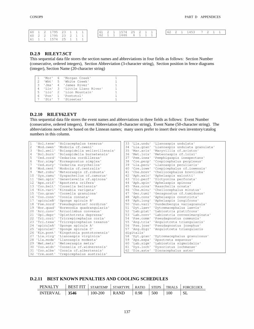
CONOP9 PART D APPENDICES

137

60 1 2 1795 23 1 1 1 60 2 2 1795 23 2 1 1 61 1 1 1574 25 1 1 1

61 2 1 1574 25 2 1 1 62 1 1 1446 6 1 1 1

62 2 1 1453 7 2 1 1

D.2.9 RILEY7.SCT This sequential data file stores the section names and abbreviations in four fields as follows: Section Number (consecutive, ordered integers), Section Abbreviation (3-character string), Section position in fence diagrams (integer), Section Name (20-character string)

1 'Mor' 6 'Morgan Creek' 1 2 'Wht' 5 'White Creek' 1 3 'Jms' 4 'James River' 1 4 'Lln' 3 'Little Llano River' 1 5 'Lio' 2 'Lion Mountain' 1 6 'Pon' 1 'Pontotol' 1 7 'Str' 7 'Streeter' 1

D.2.10 RILEY62.EVT This sequential data file stores the event names and abbreviations in three fields as follows: Event Number (consecutive, ordered integers), Event Abbreviation (8-character string), Event Name (50-character string). The abbreviations need not be based on the Linnean names; many users prefer to insert their own inventory/catalog numbers in this column. 1 'Hol.tene' 'Holcacephalus tenerus' 2 'Mod.owen' 'Modocia cf.oweni' 3 'Bol.well' 'Bolaspidella wellsvillensis' 4 'Bol.burn' 'Bolaspidella burnetensis' 5 'Ced.cord' 'Cedarina cordilleras' 6 'Kor.simp' 'Kormagnostus simplex' 7 'Ced.eury' 'Cedarina eurycheilos' 8 'Mod.cent' 'Modocia cf.centralis' 9 'Met.robu' 'Meteoraspis cf.robusta' 10 'Sys.camu' 'Syspacheilus cf.camurus' 11 'Gen.spin' 'Genevievella cf.spinosa' 12 'Aps.orif' 'Apsotreta orifera' 13 'Coo.belt' 'Coosella beltensis' 14 'Kin.vari' 'Kinsabia varigata' 15 'Coo.gran' 'Coosella granulosa' 16 'Coo.conn' 'Coosia connata' 17 'spiculeB' 'Sponge spicule B' 18 'Pse.nord' 'Pseudagnostus? nordicus' 19 'Nor.quad' 'Norwoodia quadrangularis' 20 'Arc.conv' 'Arcuolimbus convexus' 21 'Opi.depr' 'Opisthotreta depressa' 22 'Tri.cori' 'Tricrepicephalus coria' 23 'Tri.texa' 'Tricrepicephalus texanus' 24 'spiculeA' 'Sponge spicule A' 25 'spiculeC' 'Sponge spicule C' 26 'Kin.pont' 'Kingstonia pontotocensis' 27 'Lla.virg' 'Llanoaspis virginica' 28 'Lla.mode' 'Llanoaspis modesta' 29 'Met.metr' 'Metoeraspis metra' 30 'Coo.widn' 'Coosella cf.widnerensis' 31 'Coo.albe' 'Coosia cf.albertensis' 32 'Cre.aust' 'Crepicephalus australis'

33 'Lla.undu' 'Llanoaspis undulata' 34 'Lla.gran' 'Llanoaspis undulata granulata' 35 'Mar.aris' 'Maryvillia cf.ariston' 36 'Met.lois' 'Meteoraspis cf.loisi' 37 'Pem.inex' 'Pemphigaspis inexpectans' 38 'Cre.perp' 'Crepicephalus perplexus' 39 'Lla.pecu' 'Llanoaspis peculiaris' 40 'Cre.iowe' 'Crepicephalus cf.iowensis' 41 'Che.brev' 'Cheilocephalus breviloba' 42 'Aph.walc' 'Aphelaspis walcotti' 43 'Dic.perf' 'Dictyonina perforata' 44 'Aph.spin' 'Aphelaspis spinosa' 45 'Raa.orna' 'Raaschella ornata' 46 'Che.minu' 'Cheilocephalus minutus' 47 'Ger.tumi' 'Geragnostus cf.tumidosus' 48 'Aph.cons' 'Aphelaspis constricta' 49 'Aph.long' 'Aphelaspis longifrons' 50 'Dun.vari' 'Dunderbergia variagranula' 51 'Dyt.laev' 'Dytremacephalus laevis' 52 'Lab.plat' 'Labiostria platifrons' 53 'Lab.conv' 'Labiostria conveximarginata' 54 'Pse.comm' 'Pseudagnostus communis' 55 'Ang.tria' 'Angulotreta triangularis' 56 'Pse.jose' 'Pseudagnostus josephus' 57 'Ang.digi' 'Angulotreta triangularis digitalis' 58 'Dyt.gran' 'Dytremacephalus granulosus' 59 'Aps.expa' 'Apsotreta expansus' 60 'Lab.sigm' 'Labiostria sigmoidalis' 61 'Dys.loch' 'Dysoristus lochmanae' 62 'Die.aste' 'Dieracephalus aster'

D.2.11 BEST KNOWN PENALTIES AND COOLING SCHEDULES

PENALTY BEST FIT

STARTEMP

STARTYPE

RATIO

STEPS

TRIALS

FORCECOEX

INTERVAL 3546 100-200 RAND 0.98 500 100 SL

CONOP9 PART E INDEX

138

LEVEL 204 10-20 RAND 0.98 500 100 SL ORDINAL 533 10-100 RAND 0.98 500 100 SL SPATIAL 1102 20-100 RAND 0.98 500 100 SL RASCAL 186.9 10-20 RAND 0.99 500 100 SL

D.2.12 AN ABBREVIATED* SAMPLE OUTPUT TEXT FILE * Long data tables have been truncated after the first 2-3 rows. The individual section tables for sections 2 and above have been eliminated. This output was generated by an MS X.x version; so section and event tables are not in separate files.

CAMBRIAN RILEY FM> (7 sections, 62 taxa, 0 others) Optimized on Rascal Penalty RUN TIME (min) = .617 _____________________________ THE BEST WEIGHTED PENALTIES: Section Net-Penalty Possible-Penalty 1 79 pairs of 4186 possible pairs in 25 levels 2 72 pairs of 1770 possible pairs in 24 levels 3 76 pairs of 1540 possible pairs in 14 levels 4 103 pairs of 1431 possible pairs in 16 levels 5 73 pairs of 1540 possible pairs in 8 levels 6 72 pairs of 946 possible pairs in 20 levels 7 58 pairs of 780 possible pairs in 13 levels pairs: number of contradicted pairs in section possible: number of contadictable pairs in section levels: sum of levels within contradicted pairs Ordinal penalty increment is pairs Spatial penalty increment is levels Rascal penalty increment is pairs/possible Interval penalties: 1 293.00 meters ( 352.000 meters with 25 event levels ) 2 730.00 meters ( 561.000 meters with 24 event levels ) 3 467.00 meters ( 233.000 meters with 14 event levels ) 4 698.00 meters ( 340.000 meters with 16 event levels ) 5 460.00 meters ( 145.000 meters with 8 event levels ) 6 420.00 meters ( 376.000 meters with 20 event levels ) 7 733.00 meters ( 412.000 meters with 13 event levels ) BEST TOTAL PENALTY: 186.3143 Interval Penalty: 3801.0000 meters Level Penalty: 222.0000 levels Ordinal Penalty: 533.0000 pairs Spatial Penalty: 1139.0000 levels Rascal Penalty: 186.3143 Smoothness Penalty: 361.7784 meters Smoothing Factor: .0000 ______________________________________________ THE RUN PARAMETERS The initial solution - random sequence Annealing Schedule - Initial temperature: 20.000000 10% cooled: 7.283400 30% cooled: 9.659228E-01 50% cooled: 1.281005E-01 60% cooled: 4.665034E-02 70% cooled: 1.698865E-02 80% cooled: 6.186757E-03 90% cooled: 2.253031E-03 Final temperature: 8.204862E-04 Cooling ratio: 9.800000E-01 Cooling steps: 500 Trials per step: 100 Total trials: 50000 Smoothing Factor: 0.000000E+00 Neighborhood size -

CONOP9 PART E INDEX

139

big neighborhood: one random event moved to random new position Observed (sensu lato) co-existences enforced __________________________________________ SOLUTION IN BEST SEQUENCE FOR SECTION: Morgan Creek - 1 Event Type Observed Placed Extensions(3) (unweighted meters, weighted meters, levels) 59 2 1574.000 1574.000 .000 .000 0 60 2 .000 1574.000 .000 .000 0 61 2 . . . . . . .000 .000 0 3 1 .000 1222.000 .000 .000 0 2 1 .000 1222.000 .000 .000 0 observed events: 92 extended events: 18 penalized events: 18 total thickness spanned: 352.000 event spacings spanned: 114. __________________________________________ SOLUTION IN BEST SEQUENCE FOR SECTION: White Creek - 2 . . . . _________________________________________________ INDIVIDUAL EVENT EXTENSIONS IN BEST SEQUENCE Event Type Extension Penalty Sections (extension = unweighted penalty) 59 2 .00 .00 3 Aps.expa 60 2 .00 .00 1 Lab.sigm 61 2 .00 .00 1 Dys.loch . . _________________________________________________ STANDARDIZED MEASURES OF QUALITY OF SOLUTION Number of local events to be placed: 868 Number of observed local events: 402 Number of extensible local events: 357 (i.e. observed away from section end) Number of penalizable local events: 357 (and carrying non-zero weight factor) Number of contradictable local events: 370 (i.e. observed in at least 2 sections) Number of improvable local events: 325 (i.e. extensible and contradictable) Number of extended local events: 120 Number of penalized local events: 120 Penalized fraction of improvable events: .336 (if greater than 1.0, solution is NOT optimal) Total Thickness (all sections): 2419.000000 Number of Levels (all sections): 120 Average Level Spacing: 21.407080 Penalty used to Optimize: Unsmoothed penalty per observed event: 4.634684E-01 per contradictable event: 5.035521E-01 per penalizable event: 5.218887E-01 per penalized event: 1.552619 Range extensions resulting from optimization: Net Extension Distance: 3801.000000 Extension per observed event: 9.455224 Extension per contradictable event: 10.272970 Extension per extensible event: 10.647060 Extension per extended event: 31.675000 Net Extension/Total Thickness: 1.571310

CONOP9 PART E INDEX

140

Net Extension Levels: 222 Levels per observed event: 5.522388E-01 Levels per contradictable event: 6.000000E-01 Levels per extensible event: 6.218488E-01 Levels per extended event: 1.850000 Extension Levels/Total Levels: 1.850000 ______________________________________________ THE BEST PERMUTATION FOUND IS: EVENT TYPE RANK (1 is earliest) 59 2 124 Aps.expa LAD 60 2 123 Lab.sigm LAD . . . ___________________________________________ INCREMENTAL UNWEIGHTED PENALTIES, IN BEST SEQUENCE BY EVENT NUMBER AND SECTION Event Type Penalty in Sections 1 - 7 next data table, unlabelled, = C:\MSDEV\projects\CONOP9\delta.dat 59 2 .00 .00 .00 .00 .00 .00 .00 60 2 .00 .00 .00 .00 .00 .00 .00 61 2 .00 .00 .00 .00 .00 .00 .00 . . . . _____________________________________________ THE J-DIMENSIONAL LINE OF CORRELATION i.e. the best horizon placements Event Type Placed in Sections 1 - 7 next data table, unlabelled = C:\MSDEV\projects\CONOP9\albet.dat 59 2 1574.00 1808.00 1275.00 1592.00 1230.00 1655.00 1412.00 60 2 1574.00 1795.00 1275.00 1592.00 1230.00 1655.00 1412.00 61 2 1574.00 1795.00 1275.00 1592.00 1230.00 1655.00 1412.00 . . . 3-horizon SMOOTHED PLACEMENTS: Event Type Placed in Sections 1 - 7 59 2 1574.00 1801.50 1275.00 1592.00 1230.00 1655.00 1412.00 60 2 1574.00 1799.33 1275.00 1592.00 1230.00 1655.00 1412.00 61 2 1574.00 1795.00 1275.00 1592.00 1230.00 1655.00 1412.00 . . . 5-horizon SMOOTHED PLACEMENTS: Event Type Placed in Sections 1 - 7 59 2 1574.00 1799.33 1275.00 1592.00 1230.00 1655.00 1412.00 60 2 1574.00 1798.25 1275.00 1592.00 1230.00 1655.00 1412.00 61 2 1574.00 1797.60 1273.40 1592.00 1230.00 1655.00 1412.00 . . . . _____________________________________________ OBSERVED HORIZONS: Event Type Observed in Sections 1 - 7 next data table, unlabelled = C:\MSDEV\projects\CONOP9\ab.dat 59 2 1574.00 1808.00 -247.00 -42.00 1230.00 -85.00 -279.00 60 2 .00 1795.00 -247.00 -42.00 -252.00 -85.00 -279.00 . . . ______________________________________________

CONOP9 PART E INDEX

141

STANDARD COMPOSITE SECTION maximum spacing resolved in any local solution local spacings corrected for local thickness and duration of section (events spanned) also in .DAT file: Event Type Space-Below Level-Placed 2 1 .0000 1000.0000 FAD - Modocia cf.oweni 3 1 1.0963 1001.0960 FAD - Bolaspidella wellsvillensis 2 2 .0000 1001.0960 LAD - Modocia cf.oweni ______________________________________________ COEXISTENCES - next data table, unlabelled = C:\MSDEV\projects\CONOP9\coex.dat taxon 1 coexists with: 1, 0, 0, 0, 0, 6, 0, 0, 0, 0, 11, 0, 13, 14, 15, 0, 0, 0, 0, 0, 21, 22, 23, 24, 25, 0, 0, 0, 29, 0, 0, 0, 0, 0, 0, 0, 0, 0, 0, 0, 0, 0, 0, 0, 0, 0, 0, 0, 0, 0, 0, 0, 0, 0, 0, 0, 0, 0, 0, 0, 0, 62, taxon 2 coexists with: 0, 2, 3, 0, 0, 0, 0, 0, 0, 0, 0, 0, 0, 0, . . . .

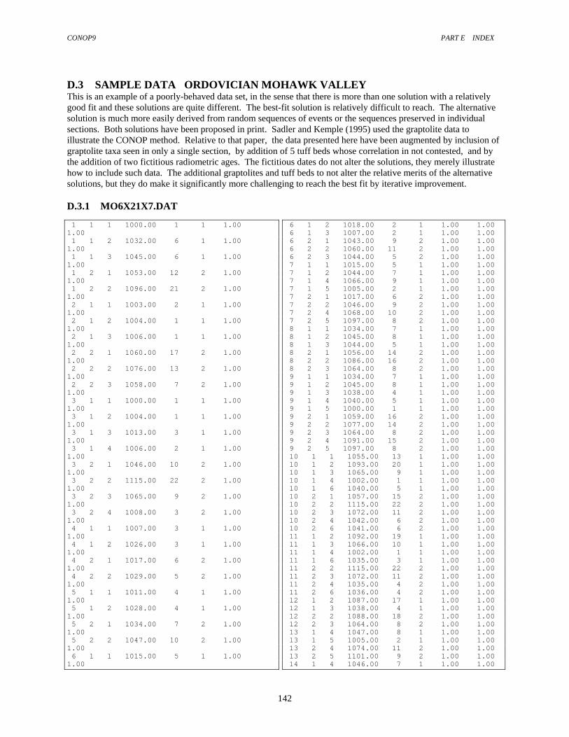
CONOP9 PART E INDEX

142

D.3 SAMPLE DATA ORDOVICIAN MOHAWK VALLEY This is an example of a poorly-behaved data set, in the sense that there is more than one solution with a relatively good fit and these solutions are quite different. The best-fit solution is relatively difficult to reach. The alternative solution is much more easily derived from random sequences of events or the sequences preserved in individual sections. Both solutions have been proposed in print. Sadler and Kemple (1995) used the graptolite data to illustrate the CONOP method. Relative to that paper, the data presented here have been augmented by inclusion of graptolite taxa seen in only a single section, by addition of 5 tuff beds whose correlation in not contested, and by the addition of two fictitious radiometric ages. The fictitious dates do not alter the solutions, they merely illustrate how to include such data. The additional graptolites and tuff beds to not alter the relative merits of the alternative solutions, but they do make it significantly more challenging to reach the best fit by iterative improvement. D.3.1 MO6X21X7.DAT 1 1 1 1000.00 1 1 1.00 1.00 1 1 2 1032.00 6 1 1.00 1.00 1 1 3 1045.00 6 1 1.00 1.00 1 2 1 1053.00 12 2 1.00 1.00 1 2 2 1096.00 21 2 1.00 1.00 2 1 1 1003.00 2 1 1.00 1.00 2 1 2 1004.00 1 1 1.00 1.00 2 1 3 1006.00 1 1 1.00 1.00 2 2 1 1060.00 17 2 1.00 1.00 2 2 2 1076.00 13 2 1.00 1.00 2 2 3 1058.00 7 2 1.00 1.00 3 1 1 1000.00 1 1 1.00 1.00 3 1 2 1004.00 1 1 1.00 1.00 3 1 3 1013.00 3 1 1.00 1.00 3 1 4 1006.00 2 1 1.00 1.00 3 2 1 1046.00 10 2 1.00 1.00 3 2 2 1115.00 22 2 1.00 1.00 3 2 3 1065.00 9 2 1.00 1.00 3 2 4 1008.00 3 2 1.00 1.00 4 1 1 1007.00 3 1 1.00 1.00 4 1 2 1026.00 3 1 1.00 1.00 4 2 1 1017.00 6 2 1.00 1.00 4 2 2 1029.00 5 2 1.00 1.00 5 1 1 1011.00 4 1 1.00 1.00 5 1 2 1028.00 4 1 1.00 1.00 5 2 1 1034.00 7 2 1.00 1.00 5 2 2 1047.00 10 2 1.00 1.00 6 1 1 1015.00 5 1 1.00 1.00

6 1 2 1018.00 2 1 1.00 1.00 6 1 3 1007.00 2 1 1.00 1.00 6 2 1 1043.00 9 2 1.00 1.00 6 2 2 1060.00 11 2 1.00 1.00 6 2 3 1044.00 5 2 1.00 1.00 7 1 1 1015.00 5 1 1.00 1.00 7 1 2 1044.00 7 1 1.00 1.00 7 1 4 1066.00 9 1 1.00 1.00 7 1 5 1005.00 2 1 1.00 1.00 7 2 1 1017.00 6 2 1.00 1.00 7 2 2 1046.00 9 2 1.00 1.00 7 2 4 1068.00 10 2 1.00 1.00 7 2 5 1097.00 8 2 1.00 1.00 8 1 1 1034.00 7 1 1.00 1.00 8 1 2 1045.00 8 1 1.00 1.00 8 1 3 1044.00 5 1 1.00 1.00 8 2 1 1056.00 14 2 1.00 1.00 8 2 2 1086.00 16 2 1.00 1.00 8 2 3 1064.00 8 2 1.00 1.00 9 1 1 1034.00 7 1 1.00 1.00 9 1 2 1045.00 8 1 1.00 1.00 9 1 3 1038.00 4 1 1.00 1.00 9 1 4 1040.00 5 1 1.00 1.00 9 1 5 1000.00 1 1 1.00 1.00 9 2 1 1059.00 16 2 1.00 1.00 9 2 2 1077.00 14 2 1.00 1.00 9 2 3 1064.00 8 2 1.00 1.00 9 2 4 1091.00 15 2 1.00 1.00 9 2 5 1097.00 8 2 1.00 1.00 10 1 1 1055.00 13 1 1.00 1.00 10 1 2 1093.00 20 1 1.00 1.00 10 1 3 1065.00 9 1 1.00 1.00 10 1 4 1002.00 1 1 1.00 1.00 10 1 6 1040.00 5 1 1.00 1.00 10 2 1 1057.00 15 2 1.00 1.00 10 2 2 1115.00 22 2 1.00 1.00 10 2 3 1072.00 11 2 1.00 1.00 10 2 4 1042.00 6 2 1.00 1.00 10 2 6 1041.00 6 2 1.00 1.00 11 1 2 1092.00 19 1 1.00 1.00 11 1 3 1066.00 10 1 1.00 1.00 11 1 4 1002.00 1 1 1.00 1.00 11 1 6 1035.00 3 1 1.00 1.00 11 2 2 1115.00 22 2 1.00 1.00 11 2 3 1072.00 11 2 1.00 1.00 11 2 4 1035.00 4 2 1.00 1.00 11 2 6 1036.00 4 2 1.00 1.00 12 1 2 1087.00 17 1 1.00 1.00 12 1 3 1038.00 4 1 1.00 1.00 12 2 2 1088.00 18 2 1.00 1.00 12 2 3 1064.00 8 2 1.00 1.00 13 1 4 1047.00 8 1 1.00 1.00 13 1 5 1005.00 2 1 1.00 1.00 13 2 4 1074.00 11 2 1.00 1.00 13 2 5 1101.00 9 2 1.00 1.00 14 1 4 1046.00 7 1 1.00 1.00

CONOP9 PART E INDEX

143

14 1 5 1000.00 1 1 1.00 1.00 14 2 4 1079.00 12 2 1.00 1.00 14 2 5 1017.00 5 2 1.00 1.00 15 1 4 1084.00 13 1 1.00 1.00 15 1 5 1041.00 7 1 1.00 1.00 15 2 4 1086.00 14 2 1.00 1.00 15 2 5 1104.00 10 2 1.00 1.00 16 1 5 1097.00 8 1 1.00 1.00 16 2 5 1112.00 11 2 1.00 1.00 17 1 5 1104.00 10 1 1.00 1.00 17 2 5 1112.00 11 2 1.00 1.00 18 1 5 1112.00 11 1 1.00 .10 18 2 5 1112.00 11 2 1.00 1.00 19 1 5 1112.00 11 1 1.00 .10 19 2 5 1112.00 11 2 1.00 1.00

20 1 5 1112.00 11 1 1.00 .10 20 2 5 1112.00 11 2 1.00 1.00 21 1 6 1021.00 1 1 1.00 1.00 21 2 6 1022.00 2 2 1.00 1.00 22 4 1 1037.00 8 0 1.00 1.00 22 4 2 1061.00 12 0 1.00 1.00 23 4 1 1050.00 11 0 1.00 1.00 23 4 2 1079.00 15 0 1.00 1.00 24 4 4 1066.00 9 0 1.00 1.00 24 4 5 1014.00 3 0 1.00 1.00 25 4 4 1068.00 10 0 1.00 1.00 25 4 5 1016.00 4 0 1.00 1.00 26 4 4 1074.00 11 0 1.00 1.00 26 4 5 1021.00 6 0 1.00 1.00 27 5 5 1016.00 4 0 452.00 453.00 28 5 2 1061.00 12 0 448.00 449.00

D.3.2 MOHAWK6.SCT

1 'Chc' 6 'Chuctanunda Creek' 1 2 'Flt' 5 'Flat Creek' 1 3 'Crg' 4 'Caroga Creek' 1 4 'Dlg' 3 'Dolgeville Dam' 1 5 'Now' 2 'Nowadaga Creek' 1 6 'Wlf' 1 'Wolf Hollow Creek' 1

D.3.3 MOHAWK28.EVT 1 'Cli.caud' 'Climacograptus caudatus' 2 'Cor.amer' 'Corynoides americanus' 3 'Rec.ampl' 'Rectograptus amplexicaulis' 4 'Amp.spc1' 'Amplexograptus sp1' 5 'Las.hark' 'Lasiograptus harknessi' 6 'Nor.brev' 'Normalograptus brevis-strictus' 7 'Dic.nich' 'Dicranograptus nicholsoni' 8 'Ort.page' 'Orthograptus pageanus' 9 'Ort.quad' 'Orthograptus quadrimucronatus' 10 'Nor.mowh' 'Normalograptus mohawkensis' 11 'Ort.rued' 'Orthograptus ruedemanni' 12 'Amp.spc2' 'Amplexograptus sp2' 13 'Cli.spin' 'Climacograptus (D.) spiniferus' 14 'Amp.prae' 'Amplexograptus praetypicalis' 15 'Gen.typi' 'Geniculograptus typicalis' 16 'Dic.flex' 'Dicellograptus cf flexuosus' 17 'Gen.pygm' 'Geniculograptus pygmaeus' 18 'Cor.ulti' 'Corynoides ultimus' 19 'Cli.doro' 'Climacograptus (D.) dorotheus' 20 'Ort.spin' 'Orthograptus spinigerus' 21 'Cor.calc' 'Corynoides calcicularis' 22 'Tuff.one' 'Tuff cluster in 1,2' 23 'Tuff.two' 'Tuff cluster in 1,2' 24 'Tuff.tre' 'Tuff triplet in 4,5' 25 'Tuff.for' 'Tuff triplet in 4,5' 26 'Tuff.fiv' 'Tuff triplet in 4,5' 27 'Rad.date' 'Fictitious date' 28 'Rad.date' 'Fictitious date'

CONOP9 PART E INDEX

144

D.4 THE CONFIGURATION FILE: CONOP9.CFG The initial portion of a typical configuration file is reproduced below. It displays the editing instructions and provides the template to repair any damage to the critical parameter list format. Numerous lines of command syntax have been removed because they are available in various sections of the manual. Notice that this .cfg file accompanied the DEC 5.1 version of the program; a few control parameters have been added to the .cfg file since then. __________________ ____CONOP9.CFG____ ___________________________________________________________________________ ____CONFIGURATION FILE and USER's GUIDE to CONOP9 CONTROL9 and CONSORT9____ ________A FAMILY OF WINDOWS PROGRAMS for STRATIGRAPHIC CORELATION__________ ____________________________VERSION DEC 5.1_______________________________ _ _ Run-Time Parameters for CONOP9.EXE - WINDOWS 95/98/NT4 QUIKWIN APPLICATION _ Copyright: Pete Sadler, Jan22/2001 - sadler@ucrac1.ucr.edu _ ___________________________________________________________________________ _1. EDITABLE PARAMETERS_______________________________________________ _______________________________________________________________ ____1.1 THE INPUT DATA____________________________________ &getinn PROJECT='RILEY (7 sections, 62 taxa, 9 others)' SECTIONS=7 TAXA=62 EVENTS=9 MAX_LEVELS=100 MAX_LABELS=15 LOADFILE='rile7x62x9.dat' PREPFILE='rile7x62x9.dis' SECTFILE='riley7.sct' LABELFILE='riley.lbl' EVENTFILE='riley66.evt' BESTKNOWN=3546.00 / ____1.2 PARAMETERS THAT ALTER THE BEST SOLUTION___________ &getans PENALTY='interval' LETCONTRACT='FILE' WEIGHTING=’ON’ USENEGATIVE='OFF' NEARENOUGH=0.0 EXCLUSIVES='NO' FORCECOEX='sl' HOMERANGE='sl' SMOOTHER=0.00 SQUEEZER=0.00 SHRINKER=0.00 TEASER=0.00 STACKER='COEX' / ____1.3 PARAMETERS THAT INFLUENCE EFFICIENCY______________ ________OF THE SEARCH FOR THE BEST SOLUTION_______________ &getrun SOLVER='anneal' STEPS=500

CONOP9 PART E INDEX

145

TRIALS=100 STARTEMP=200 RATIO=0.98 HOODSIZE='big' STARTYPE='rand' STARTSECT=1 STARTEVENT=0 SHOWMOVIES='ON' TRAJECTORY='ALL' VIDEOMODE='SVGA' PAUSES='ON' CURVFILE='riley.grd' CRV2FILE='riley.gr2' / ____1.4 PARAMETERS THAT DETERMINE THE NATURE______________ _______ AND THE LOCATION OF THE OUTPUT DATA_______________ &getout COLUMNS=7 UNLOADMAIN='outmain.txt' FITS_OUT='ON' CNFG_OUT='ON' SEQN_OUT='ON' INCR_OUT='OFF' LOC_OUT='OFF' OBS_OUT='ON' COMP_OUT='OFF' UNLOADSECT='outsect.txt' SECT_OUT='ON' UNLOADEVNT='outevnt.txt' EVNT_OUT='OFF' COEX_OUT='OFF' RUNLOGFILE='runlog.txt' CULLFILE='cull.txt' SOLNLIST='OFFsolution.sln' STARTFILE='soln.dat' STEPFILE='OFFstepsoln.dat' BESTARTFILE='bestsoln.dat' COMPOSFILE='cmpst.dat' COMPOSNMBR=1 COMPOSTYPE='ZMX' OBSDFILE='ab.dat' PLCDFILE='albet.dat' EXTNFILE='delta.dat' COEXISTFILE='coex.dat' ORDERFILE='ordr.dat' / __________________________________________________________ __________________________________________________________________ __1.5 WARNING_______________________________________________________________ _ EDIT SECTIONS 1.1 to 1.4 ONLY AS INSTRUCTED BELOW. _ Text from section 1.5 to the end may be printed and deleted; _ it serves as a users' reference manual. _ __1.6 NOTE TO CONOP3 VETERANS______________________________________ _ This file has fewer editable parameters than CONOP3.CFG _ The "lost" options are now accessible via menus at run time. _ The menus allow repeated display of output graphics and _ use of Windows95/NT editing and graphics capture options. _ __1.7 OPERATING SYSTEMS______________________________________________________

CONOP9 PART E INDEX

146

_ Early versions of CONOP9 were compiled using MICROSOFT Fortran Power _ Station. It could not handle allocatable arrays in Windows NT 4.0. _ This version has been rewritten for the DEC Visual Fortran compiler. _ The allocatable arrays ensure that the arrays are no larger than needed _ for the problem at hand. _ __1.8 HARDWARE ASSUMPTIONS___________________________________________________ _ The CONOP9 program was developed on a laptop with the following rather _ modest settings: _ Windows 95 _ 32Mb RAM _ Pentium 233Mhz _ 800 x 600 screen resolution _ High Color (16 bit) graphics setting _ _ Other Processors used successfully: _ Intel Pentium II _ Intel Pentium III 600Mhz _ Intel Celeron 266 Mhz and 600Mhz _ Intel Pentium IV 1700Mkz _ _ Macintosh runs: _ i-mac with PC-emulator _ _ On desktop computers running Windows NT higher screen resolutions are _ preferable -- more taxa fit into the run-time graphics. _ _ Several output files exceed floppy disk capacity when the problem _ exceeds trivial sizes. The output paths should not be set to 1.44Mb _ drives until prior runs with the same parameters have established that _ the files will fit. The size of the output files increases with the size _ of the problem. Some grow proportionally with the number of sections; _ other file sizes reflect the number of events. _ __1.9 MEMORY REQUIREMENTS____________________________________________________ _ _ Some of the largest known successful runs - _ _ CONOP9.EXE _ 169 sections, 425 taxa, 22 unpaired events _ - Win'95 and 32Mb RAM _ - NT-4.0 and 128Mb RAM _ _ 21 sections, 177 taxa _ - 5 parallel runs on NT-4.0 and 128Mb RAM _ _ 97 sections, 376 taxa _ - with Word '97 on Win'95 and 32Mb RAM _ - 2 parallel runs with Dbase 5.0 on Win'95 and 32Mb RAM _ _ [CONOP3.EXE] _ 27 sections, 133 taxa _ - Win 3.1 and 8Mb RAM _ _ _ CONOP9 seems to take aggressive charge of Windows memory resources. _ This is probably because the program loops in memory without any disk _ activity or pauses for keyboard interaction. WIndows seems to have _ fewer opportunities to query parallel tasks. Consequently, screen _ savers run very slowly (i.e. appear to be frozen) and mouse movements

CONOP9 PART E INDEX

147

_ restore the CONOP screen very sluggishly. Don't panic; revel in the _ efficiency! As successive parallel runs of CONOP9 are launched, it _ becomes increasingly difficult to get Windows attention and start the _ next one. Avoid this snag by putting each run in "Suspend" mode after _ launching; "Resume" them after all have started. _ _ Although the array sizes are allocated at run time, the stack size must _ be set during compilation. Currently the value is 4Mb. This has _ accommodated data sets up to 140 sections by 425 taxa and a high _ resolution screen. If the stack size is exeeded the program will stop _ with a fatal error labelled "Stack Overflow." The error message will _ appear during the initial data-loading cycle, if the input file is too _ large for the stack. A large data set that uses most of the stack may _ cause the error to appear during preparation of post-run graphics -- _ some of these routines set up additional arrays. One large post-run _ array stores screen colors for the 2-section LOCs. Another large array _ is needed to calculate confidence intervals. Although these post-run _ errors cause the program to terminate, the output files should be _ intact. A run of 1-step and 1-trial, starting from file, will quickly _ return to the previous.solution. In order to gain access to all the _ graphic options for an oversized data set, request a recompilation _ with larger stack size. _ ____________________________________________________________________________ __2. THE PURPOSE of CONOP9.CFG______________________________________________ _ _ _ 1. User-Editable Run-Time Parameters for CONOP9.EXE _ - which solves a stratigraphic correlation _ problem based on the data in LOADFILE _ using instructions from CONOP9.CFG _ and writes answers to UNLOADMAIN, _ +/- UNLOADSECT, +/-UNLOADEVNT, _ +/- RUNLOGFILE _ _ 2. Also used by CONSORT9.EXE _ - which takes the preliminary PREPFILE listing _ and expands it by assigning the _ sequential numbers to collecting LEVELS, _ expanding top-only and bottom-only taxon entries, _ sorting the sequence of records, _ and writing the LOADFILE for CONOP9 to use. _ Also provides options to edit the weighting factors _ in LOADFILE. i.e. all input preparation. _ _ 3. Also used by CONTROL9.EXE _ - which examines all aspects of the LOADFILE data _ that do not require finding the best solution. _ CONTROL9 has a run-time, drop dowm menu of _ options to analyze the input data set or _ map the penalty landscape. _ - the CONTROL9 options fall into three categories: _ "standard," "advanced," and "experimental." _ Sadler uses the "experimental" options to map _ the problem landscape; they have very long _ run-times and are not at all user-friendly. _ _ _ LOAD THIS FILE (CONOP9.CFG) TO SAME DIRECTORY AS CONOP9.EXE, _ CONSORT9.EXE

CONOP9 PART E INDEX

148

_ and CONTROL9.EXE _ _ The name of this configuration file and the assumption that it _ resides with the EXE files is hard-coded into the EXE files. _ This condition cannot be altered except at source code level. _ _ Edit this file to set all the run-time parameters for CONOP9.EXE _ Instructions are given below. For more explanation and to cite _ the working principles of the CONOP program family: _ _ Kemple, W.G., Sadler, P.M., and Strauss, D.J., 1995, Extending _ Graphic correlation to many dimensions: stratigraphic correlation _ as constrained optimization: SEPM Special Publication 53, p.65-82. _ _ To cite this particular version, refer to this file: _ _ Sadler, P.M., 1999, User's guide to CONOP9, CONTROL9, and CONSORT9' _ a family of Windows 95/NT programs for stratigraphic correlation, _ version dec3.0, distributed by author. _ _ suggestions to sadler@ucrac1,ucr.edu ___________________________________________________________________________ __3. EDITING INSTRUCTIONS__________________________________________________ _ _ EDIT only the portion of configuration command lines after "=" _ DO NOT EDIT lines that mark top (&get???) and base (/) of lists; _ intervening lines may be placed in a different order. _ Editing or deleting lines that begin with "_" will not _ influence the run-time performance. _ Command lines start with " ", rather than "_" _ Most command line options may be typed in upper or lower case, _ but not in a mixture of cases. If in doubt, use upper case only. _ Command syntax and editing instructions follow in two sections;: _ 3.1 gives a beginners guide to the bells and whistles that matter _ and those that do not _ 4.1 starts into the full command syntax _ __________________________________ ____3.1 BEGINNER's COMMAND SYNTAX _

THE REST OF THIS FILE IS NOT REPRODUCED; IT IS COVERED BY MANY SECTIONS OF THIS MANUAL

CONOP9 PART E INDEX

149

E INDEX Items in UPPER CASE (except for standard abbreviations) are CONOP parameter names or CONOP parameter options or file names.

& &GETANS, 16, 33, 140 &GETINN, 16, 29, 140 &GETOUT, 17, 63, 141 &GETRUN, 16, 48, 140

A Accumulation Rate, 34, 35, 69, 71, 72 Animated Range Chart, 20, 21, 22, 42, 43, 52, 57, 58, 61,

62, 69, 120, 123 ANNEAL, 14, 17, 48, 50, 51, 53 ASCII, 12, 18, 24, 25, 26, 27, 28

B Back-up, 62, 119 Base of Section, 18, 67 Best Fit, 33, 43, 44, 50, 53, 57, 60, 73, 77, 82, 83, 85, 86,

87, 97, 104, 106, 123, 138 Best Fit Curve, 58, 77, 81 Best Fit Interval, 50, 60, 73, 77, 83, 86, 106, 123 BESTARTFILE, 15, 17, 56, 66, 67, 141 BESTKNOWN, 14, 16, 33, 62, 140 Boltzmann, 48

C Cambrian, 131, 134 Caved Ranges, 23, 24 CGA, 17, 60 Cladistics, 11 CNFG_OUT, 15, 17, 64, 141 COEX_OUT, 15, 17, 65, 141 Coexistence, 19, 20, 21, 22, 37, 39, 40, 41, 42, 43, 46, 47,

48, 55, 56, 59, 63, 65, 73, 87, 114, 115, 116, 124 Coexistence Matrix, 19, 22, 41, 42, 43, 48, 55, 63, 73, 116 COEXISTFILE, 15, 17, 42, 73, 141 COLUMNS, 15, 17, 63, 141 COMP_OUT, 15, 17, 64, 141 COMPOSFILE, 15, 17, 68, 69, 141 Composite Section, 24, 26, 30, 31, 38, 64, 68, 69, 70, 71,

72, 85, 86, 87, 95, 97, 98, 106 COMPOSNMBR, 15, 17, 69, 141 COMPOSTYPE, 15, 17, 64, 68, 69, 70, 71, 72, 86, 106,

141 CONOP.EXE, 29, 63, 122 CONOP2.EXE, 122

CONOP3.CFG, 90, 94, 97, 98, 115, 116, 117, 118, 122, 141

CONOP3.EXE, 122, 142 CONOP9.CFG, 12, 13, 14, 16, 24, 29, 74, 108, 117, 119,

120, 123, 140, 143 CONOP9.EXE, 12, 13, 14, 19, 31, 63, 66, 67, 74, 120, 122,

123, 140, 142, 143, 144 CONSORT3.EXE, 122 CONSORT9.EXE, 12, 13, 18, 19, 20, 21, 29, 30, 126, 127,

143 Constraint, 34, 40, 41, 42, 43, 45, 47 Constraint - optional, 34, 42, 45, 47 Constraints, 37, 41, 43, 54, 77 CONTROL3.EXE, 122 CONTROL9.EXE, 12, 41, 63, 64, 126, 127, 143 Cooling Schedule, 45, 48, 49, 51, 53, 54, 59, 61, 104, 123 CRV2FILE, 15, 17, 60, 61, 63, 74, 120, 141 CULLFILE, 15, 17, 67, 141 CURVFILE, 15, 17, 33, 58, 60, 61, 62, 63, 67, 73, 74, 97,

106, 119, 141 CUSTOM, 66

D Diversity, 43, 57, 62, 69, 72, 85, 86, 87, 124

E Economy of Fit, 34, 36 Event Dictionary, 14, 31, 32, 33, 57 Event Number, 18, 133 Event Type, 18, 136, 137 EVENTFILE, 14, 16, 25, 26, 27, 28, 120, 140 EVENTS, 14, 16, 20, 21, 22, 23, 29, 112, 140 Evidence – negative, 43, 44, 45, 46 EVNT_OUT, 15, 17, 65, 141 EXCLUSIVES, 40 Exit, 120 Extinction, 70, 86, 87, 123, 124 EXTNFILE, 15, 17, 68, 141

F FAD, 18, 19, 20, 21, 22, 23, 24, 29, 32, 34, 42, 44, 46, 47,

59, 77, 137 First Appearance Datum (FAD), 18, 19, 20, 21, 22, 23, 24,

26, 27, 29, 32, 34, 42, 44, 46, 47, 57, 59, 77, 88, 103, 104, 105, 106, 107, 108, 111, 112, 113, 114, 115, 117, 137

FITS_OUT, 15, 17, 64, 141

CONOP9 PART E INDEX

150

Font, 29, 63, 75, 80, 123, 126 FORCECOEX, 14, 16, 35, 40, 41, 42, 75, 79, 134, 140

G Gaps, 13, 18, 53 GRAPHFONT, 75, 80 Graphic Correlation, 4, 36, 109, 131, 144 Graptolites, 138 GREEDY, 17, 48, 49, 50, 53 Greedy Algorithm, 39, 45, 49, 50, 53, 118

H Heuristic, 33, 48, 50, 58 Hiatus, 18, 22, 35, 108, 109 HOMERANGE, 14, 16, 43, 120, 140 HOODSIZE, 15, 17, 48, 49, 50, 51, 54, 55, 141 Horizon Value, 18

I INCL, 16, 44, 46, 47, 48 INCR_OUT, 15, 17, 64, 141 INTERVAL, 16, 34, 35, 36, 38, 49, 52, 134

L LAD, 19, 20, 21, 22, 23, 24, 29, 32, 34, 42, 44, 46, 47, 59,

77, 136, 137 Last Appearance Datum (LAD), 18, 19, 20, 21, 22, 23, 24,

26, 27, 29, 32, 34, 42, 44, 46, 47, 57, 59, 77, 88, 103, 104, 105, 106, 107, 108, 111, 112, 113, 114, 115, 117, 136, 137

LETCONTRACT, 14, 16, 36, 42, 43, 140 LEVEL, 14, 16, 23, 24, 30, 34, 35, 36, 48, 49, 52, 134 Line of Correlation, 15, 17, 44, 45, 64, 68, 94, 97, 108,

109, 141 LOADFILE, 12, 13, 14, 16, 18, 24, 25, 26, 27, 28, 29, 30,

31, 32, 66, 67, 72, 110, 140, 143 LOC_OUT, 15, 17, 64, 141 Locating Task, 33, 34, 36, 37, 38, 42, 46, 47, 64, 68, 69,

70, 71, 97, 98 Log Off, 75, 79, 118 LOOP, 51, 57, 59, 60, 123, 142

M MAPPER, 115, 116, 117, 118 Marker Beds, 18, 21, 57 Menu, 12, 19, 20, 22, 60, 65, 67, 73, 75, 77, 79, 86, 88,

102, 103, 108, 109, 118, 120, 123, 126, 143 Minimum - global, 53 Minimum – local, 45, 49, 51, 52, 53, 54, 81, 110, 118 MISFIT, 33, 34, 36, 37, 38, 39, 40, 43, 44, 49, 50, 52, 61,

64, 74, 81, 82, 83, 86, 97, 117, 123, 126, 131 Mohawk Valley, 20, 21, 138 Moves – permitted, 19

N Navigation Keys, 75, 79, 80, 83, 97, 110 Neighborhood, 48, 49, 50, 51, 54, 55, 57, 58, 59, 97, 135 Neighborhood - big, 15, 17, 54, 55, 56, 58, 59, 135 Neighborhood - double, 17, 54, 55, 56, 58, 59 Neighborhood - small, 17, 51, 54, 55, 58, 59, 97

O Objective Function, 33, 52, 65 OBS_OUT, 15, 17, 64, 141 OBSDFILE, 15, 17, 67, 68, 69, 73, 141 OLAP, 16, 44, 46, 47, 48, 53 Optimization, 29, 33, 34, 44, 47, 49, 50, 58, 136 Optimization - constrained, 68, 144 Optimization – inner, 34, 44 Optimization – outer, 33, 44 ORDERFILE, 15, 17, 141 ORDINAL, 16, 34, 35, 36, 37, 47, 52, 57, 70, 86, 134 Ordovician, 138 Origination, 70, 71, 86, 87, 123, 124

P Pairwise Contradictions, 74, 85, 87 Partial Reoptimization - full, 48, 50, 51, 54, 55 Partial Reoptimization - partial, 50, 51, 54, 55 PAUSES, 15, 17, 51, 56, 57, 60, 61, 62, 81, 102, 120, 121,

123, 124, 141 PENALTY, 14, 16, 34, 35, 36, 37, 52, 134, 140 Penalty - best, 59, 77, 102, 109 Penalty – best, 57, 58, 59 Penalty – best, 97 Penalty – best, 97 Penalty – best, 103 Penalty – best, 104 Penalty – best, 104 Penalty – best, 105 Penalty – best, 106 Penalty – best, 107 Penalty – best, 107 Penalty - initial, 52, 55, 59 Penalty - secondary, 43, 44, 45, 46 PLCDFILE, 15, 17, 67, 68, 141 PREPFILE, 12, 13, 14, 16, 18, 21, 23, 24, 25, 26, 27, 28,

29, 30, 31, 121, 140, 143 PROJECT, 14, 16, 29, 140

Q Quenching, 49, 51, 52, 53

R Radiometric Dates, 18, 19, 21, 23, 29, 72, 138 RAND, 15, 17, 55, 56, 57, 117, 134 Range Chart, 4, 42, 43, 52, 57, 69, 90, 97, 105, 106, 115,

120 Range Contraction, 23, 24, 34, 37, 42, 43, 90, 118

CONOP9 PART E INDEX

151

Range Extension, 19, 22, 34, 35, 36, 43, 44, 48, 68, 85, 86, 90, 94, 112, 113, 123, 136

RASC, 36, 37, 42, 77 RASCAL, 16, 34, 37, 47, 52, 134 RATIO, 15, 17, 48, 49, 52, 53, 54, 58, 134, 141 Regression, 33, 49 Regression - linear, 33, 49 Relaxed Fit, 39, 60, 62, 63, 83, 106, 123 Relaxed Fit Curve, 39, 58, 60, 62, 63, 77, 81, 106, 123 Reoptimization, 4, 44, 48, 50, 51, 54, 55 Reoptimization - full, 48, 50, 51, 54, 55 Reoptimization – full, 48 Reoptimization – full, 50 Reoptimization – full, 51 Reoptimization – full, 54 Reoptimization – full, 54 Reoptimization – full, 54 Reoptimization – full, 55 Reoptimization – full, 55 Reoptimization - partial, 50, 51, 54, 55 Reworked Ranges, 24 Riley Formation, 20, 105, 106, 107, 110, 111, 112, 114,

131, 134, 140 ROYAL, 16, 34, 37, 42 RUNLOGFILE, 12, 15, 17, 74, 77, 83, 119, 141, 143

S SECT_OUT, 15, 17, 65, 141 SECTFILE, 14, 16, 24, 26, 31, 32, 69, 72, 120, 140 Section Dictionary, 14, 31 Section Number, 18, 133 SEQN_OUT, 15, 17, 64, 141 Sequencing Task, 33, 35, 36, 64, 66 Seriation, 3, 14, 19, 39, 43, 44, 47, 48, 49, 50, 69 SHOWMOVIES, 15, 17, 50, 53, 57, 58, 59, 60, 62, 73, 81,

124, 141 SHRINK, 17, 45, 48, 50, 53 SHRINKER, 14, 16, 44, 45, 46, 140 Simulated Annealing, 4, 36, 40, 48 Simulated Tempering, 49, 51, 52, 53, 58, 59, 60, 81 SMOOTHER, 14, 16, 44, 45, 46, 140 SOLNLIST, 15, 17, 69, 72, 141 Solution – final, 22, 38 Solution – initial, 41, 54, 55, 56, 59, 66, 67, 74, 134 Solution – optimal, 40, 49, 53, 65, 67, 97 Solution – suboptimal, 49, 50, 53, 59, 60, 67, 97 SOLVER, 14, 17, 44, 45, 46, 47, 48, 49, 50, 51, 52, 140 Spacing Task, 24, 31, 33, 64, 69, 72 SPATIAL, 16, 34, 36, 47, 52, 134 SQUEAL, 17, 45, 48, 50, 53 SQUEEZE, 17, 45, 48, 49, 53 STACK, 17, 45, 47, 48, 49, 53 STACKER, 14, 16, 37, 44, 46, 47, 48, 49, 53, 120, 140

STANDARD COMPOSITE SECTION, 68, 70, 72 STARTEVENT, 15, 17, 27, 57, 58, 59, 141 STARTFILE, 15, 17, 56, 66, 67, 141 STARTSECT, 15, 17, 56, 57, 141 STEAL, 17, 44, 45, 47, 48, 49 STEPFILE, 15, 17, 56, 66, 121, 141 STEPS, 14, 17, 48, 49, 51, 53, 56, 58, 61, 66, 75, 79, 110,

117, 121, 134, 140 SVGA, 15, 17, 57, 60, 122, 123, 141

T TAXA, 14, 16, 29, 140 TEASER, 14, 16, 44, 45, 46, 48, 140 Temperature –, 48, 49, 53 Temperature – final, 51, 52, 53, 135 Temperature – initial, 134 Time Averaging, 41 Time Scales, 69, 72 Times New Roman, 75, 80, 123, 126 TRAJECTORY, 15, 17, 59, 141 TRIALS, 14, 17, 48, 49, 51, 52, 53, 54, 56, 58, 61, 66, 75,

79, 110, 117, 121, 134, 141

U UNLOADEVNT, 12, 15, 17, 63, 65, 141, 143 UNLOADMAIN, 12, 15, 17, 63, 64, 120, 141, 143 UNLOADSECT, 12, 15, 17, 63, 64, 120, 141, 143 USENEGATIVE, 14, 16, 43, 44, 120, 140

V VGA, 17, 60, 122, 123 VIDEOMODE, 15, 17, 60, 141

W Weight – down, 19 Weight – up, 19 Weight – zero, 20, 22 Weighting, 13, 19, 20, 22, 29, 39, 40, 42, 44, 45, 46, 65,

124, 131, 143 WEIGHTING, 14, 16, 39, 40, 65, 120, 124, 140 Windows 95, 60, 75, 80, 120, 121, 122, 123, 126, 141, 142,

144 Windows 98, 60, 120, 121 Windows NT, 120, 122, 123, 142

Z Z-score, 68, 69, 70, 71, 72