a new approach to raising social security’s ... -...

A NEW APPROACH TO RAISING SOCIAL SECURITY’S

EARLIEST ELIGIBILITY AGE?

Kelly Haverstick, Margarita Sapozhnikov, Robert Triest, and Natalia Zhivan*

CRR WP 2007-19

Released: October 2007

Draft Submitted: October 2007

Center for Retirement Research at Boston College

Hovey House

140 Commonwealth Avenue

Chestnut Hill, MA 02467

Tel: 617-552-1762 Fax: 617-552-0191

http://www.bc.edu/crr

* Kelly Haverstick is a research economist at the Center for Retirement Research at

Boston College (CRR). Margarita Sapozhnikov is a graduate research assistant at the

CRR. Robert Triest is a visiting scholar at the CRR. Natalia Zhivan is a graduate

research assistant at the CRR. The research reported herein was performed pursuant to a

grant from the U.S. Social Security Administration (SSA) funded as part of the

Retirement Research Consortium. The opinions and conclusions expressed are solely

those of the authors and should not be construed as representing the opinions or policy of

SSA, any agency of the Federal Government, or Boston College.

© 2007, by Kelly Haverstick, Margarita Sapozhnikov, Robert Triest, and Natalia Zhivan.

All rights reserved. Short sections of text, not to exceed two paragraphs, may be quoted

without explicit permission provided that full credit, including © notice, is given to the

source.

About the Center for Retirement Research The Center for Retirement Research at Boston College, part of a consortium that includes parallel centers at the University of Michigan and the National Bureau of Economic Research, was established in 1998 through a grant from the Social Security Administration. The Center’s mission is to produce first-class research and forge a strong link between the academic community and decision makers in the public and private sectors around an issue of critical importance to the nation’s future. To achieve this mission, the Center sponsors a wide variety of research projects, transmits new findings to a broad audience, trains new scholars, and broadens access to valuable data sources.

Center for Retirement Research at Boston College Hovey House

140 Commonwealth Avenue Chestnut Hill, MA 02467

phone: 617-552-1762 fax: 617-552-0191 e-mail: [email protected]

www.bc.edu/crr

Affiliated Institutions: American Enterprise Institute

The Brookings Institution Center for Strategic and International Studies

Massachusetts Institute of Technology Syracuse University

Urban Institute

Abstract

While Social Security’s Normal Retirement Age (NRA) is increasing to 67, the Earliest

Eligibility Age (EEA) remains at 62. Similar plans to increase the EEA raise concerns

that they would create excessive hardship on workers that are worn-out or in bad health.

One simple rule to increase the EEA is to tie an increase to the number of quarters of

covered earnings. Such a provision would allow those with long worklives —

presumably the less educated and lower paid — to quit earlier. We provide evidence that

this simple rule would not satisfy the goal of preventing undue hardship on certain

workers. Thus, this paper considers an alternative policy that ties an increase in the EEA

to individuals’ Average Indexed Monthly Earnings (AIME). We show that allowing

workers with low AIME to continue to be eligible to receive benefits at age 62 has

promise as a policy to protect workers who have low earnings and are in poor health from

hardship associated with an increase in the EEA.

I. Introduction

Social Security’s Normal Retirement Age (NRA) is currently rising from age 65

to age 67. An individual must wait until the NRA to claim full benefits; benefits claimed

at an earlier age are actuarially reduced. Despite the rise in the NRA, the Earliest

Eligibility Age (EEA) — the earliest age individuals can claim reduced benefits —

remains at 62. A question facing policymakers is whether the EEA should be increased

to 64 to match the increase in the NRA. Increasing the EEA would not alter Social

Security’s financial state since benefit reductions for a person with average life

expectancy are actuarially fair — benefits are lowered to offset the longer claiming

period. However, a rise in the EEA would protect workers from facing an increased risk

of inadequate benefits if they or their spouse live beyond average life expectancy.

Raising the EEA involves making a tradeoff between ensuring retirement income

adequacy and insuring workers against the prospect that they will find it difficult to work

or find jobs as they age. As the NRA increases, there is a reduction in the benefits

payable to a worker claiming at any age below the NRA. This reduction raises the

concern that workers may myopically claim benefits too early, making it difficult for

them to maintain their living standard during retirement. The prospect of future increases

in Medicare premiums and out-of-pocket medical expenses imply that this problem will

likely grow in importance, especially in the case of widows or widowers relying on

survivors’ benefits as their primary source of income.

Increasing the EEA prevents workers from putting their future standard of living

at risk, but it does so at the cost of potentially causing hardship for those workers who

find it difficult to work at ages younger that the NRA. Individuals who have physically

demanding jobs may find work to be increasingly onerous as they age, and yet not have

health problems serious enough to qualify for disability benefits. If such individuals lack

adequate private pension benefits or other financial resources, then an increase in the

EEA would require them to either rely on inadequate income or prolong their working

lives when they would instead prefer to retire.

To avoid hurting those unable to work, some have proposed tying the EEA to the

length of a worker’s labor force participation. The idea of differentiation based on labor

2

force participation rates has an intuitive appeal and is easy to implement. Those who

went to college and thus delayed entry into the workforce usually have a safer working

environment, higher incomes, better health, and longer life expectancies, and thus can

remain in the labor force more easily. While health status, ability to work, or even level

of education are not directly observed by the Social Security Administration, information

on earnings and number of quarters of covered earnings are routinely used to determine

eligibility and the level of monthly benefits.

One simple proposed scheme would give workers an option of retiring at 62 and

claiming unreduced benefits if they have spent at least 35 years in the labor force.

Everybody else’s EEA would be moved to 64. Credit years would be assigned to women

to reflect the number of years spent caring for young children.

Our analysis demonstrates that policy rules that tie labor force participation to

eligibility for unreduced benefits at age 62 fail to help those who are in poor health.

Unhealthy workers are simply unable to obtain 35 years of labor force participation,

while workers in good health satisfy the proposed test for eligibility. Healthy workers,

however, tend to postpone claiming and retirement until a later age regardless of the

EEA. Thus, tying the EEA to the length of a worker’s labor force participation would not

help many individuals who are unable to work due to poor health or an inability to find

jobs in their 60s.

While the number of covered quarters is a poor measure of health status, earnings

are a good predictor of health, wealth, and job prospects later in life. Our analysis shows

that tying the EEA to the Average Indexed Monthly Earnings (AIME) may have some

potential. Admittedly, this method is more complex (with decisions to be made

concerning cutoff values for eligibility), so further research is necessary to determine the

feasibility of such a rule.

This paper is organized as follows. Section II discusses the data used and

provides descriptive statistics for the sample. Section III summarizes the results of

bivariate probit regressions of the decisions to claim early benefits and to exit the labor

force. Section IV puts forth a simple rule for raising the EEA and considers its effects,

including why it does not meet our goal of protecting the most vulnerable workers. This

3

section then describes an alternative rule to raise the EEA based on a worker’s earnings;

this approach would better satisfy our main objective. Section V concludes.

II. Data and Sample

To consider potential rules for increasing the EEA, this analysis uses the RAND

public version of the Health and Retirement Study (HRS) and the SSA Administrative

Data (SSAA), which contain seven waves of data (1992-2004).1 The sample selection

process follows that of Panis et al. (2002) and is shown in Figure 1. We begin with

10,560 individuals. We require that respondents reach the age of 63 by the 2004 wave,

have the Social Security benefit type available, have quarters of covered earnings

information, are not widow(er)s, do not receive care for a dependent child under the age

of 16, and do not clearly misrepresent their information.2 This leaves a final sample of

3,277 individuals.

Each individual in our sample is classified into one of six categories based on the

claim of Social Security benefits.3 These categories are determined using the “Type of

benefits received from Social Security” and the “Type of supplemental (other) benefits

received from Social Security” variables in the SSAA data:

• “Takers”: Individuals who receive their own Old-Age and Survivors

Insurance (OASI) benefits at 62 years of age;

• “Postponers”: Individuals who are eligible for their own early OASI

benefits but claim after age 62;

• “Spousal Takers”: Individuals who receive OASI spousal benefits starting

at age 62;

• “Spousal Postponers”: Individuals who are eligible for early OASI spousal

benefits but claim after age 62;

• “Ineligibles”: Individuals who do not qualify for OASI benefits; and

1 Specifically, we use the HRS Cohort: Respondent Earnings and Benefits data file. 2Widow(er)s become eligible for benefits at the age of 60 and are not directly affected by a higher EEA. Thus, 478 observations identified as widow(er)s were excluded. 3 These categories were defined using the method of Panis et al. (2002).

4

• “DI claimants”: Individuals who receive Disability Insurance (DI)

benefits.

Table 1 shows the distribution of claimant types by gender. With the inclusion of

the 2000, 2002, and 2004 waves of data, these percentages are not statistically different

from those reported by Panis et al. (2002) with two exceptions due to female takers who

have dual entitlement.4 Our method classifies all individuals with dual entitlement into

the spousal benefits category.5 Table 2 shows the breakdown in the spousal benefit

category between “dual benefit” claimants and “spousal benefit only” claimants for

females and for the entire sample. Most individuals classified as spousal benefit takers

have dual entitlement rather than only spousal benefits. This variation in classification,

rather than a difference in the composition of the two samples, appears to be the reason

for the discrepancy in the proportions in these two groups.

Characteristics of EEA Claimants

Once individuals are classified into claimant categories, we can consider the

descriptive characteristics of the takers compared to the postponers. In determining a rule

for increasing the EEA, we begin with observing the characteristics of the individuals

who claim benefits at the current EEA, 62, to gain insight on the people affected by the

increase.

Table 3 contains summary statistics on the number of covered earnings quarters,

health, physical job, wealth, pension coverage, and education for OASI worker claimants

(based on their own work history). These summary statistics are reported by gender and

claimant type (taker or postponer). The first variable of interest, number of quarters of

covered earnings by age 62, shows no statistical differences between takers and

postponers within each gender. As expected, there are statistical differences in the means

and medians between the genders, with higher values for males than for females.

4 See Table 3.2 in Panis et al. (2002) for comparison proportions. 5 “Under the dual entitlement provision, if a person is entitled to a larger Social Security benefit as a worker than as a spouse, no spouse’s benefit is payable because the person is not considered dependent on the other spouse. Similarly, if the benefit payable as a spouse exceeds the worker’s benefit for a person, then the spouse’s benefit is offset by the amount of the worker’s benefit. As a result of the dual entitlement provision, nearly 6 million beneficiaries receive reduced benefits as a spouse — meaning they receive the equivalent of their worker’s benefit or their spouse’s benefit, whichever is higher.” See U.S. Social Security Administration (2000).

5

The next two rows of the table show that there are substantial differences in the

health of takers and postponers. Of those who report poor health at age 63, 40 percent

were male takers (compared to 34 percent of the entire sample), 25 percent were male

postponers (compared to 33 percent), 24 percent were female takers (compared to 19

percent), and 10 percent were female postponers (compared to 14 percent overall).

Individuals who report poor health or job-limiting health are more likely to claim early

benefits. The opposite is true for those reporting having a physical job, as they were less

likely to be takers and more likely to be postponers. However, this finding may be

misleading since having a physical job is measured at age 63. Thus, if an individual has a

job (whether physical or not) at age 63, he is probably less likely to have already claimed

Social Security benefits.6

Male takers have lower mean and median non-housing wealth than do male

postponers, while the mean and median for females indicate that wealthier women claim

benefits early. For both males and females, there is more variance in the takers’ wealth

than in the postponers’ wealth, indicating that the group retiring later is more

homogeneous with respect to wealth. The heterogeneity in wealth among those taking

benefits early is suggestive that early takers are a mix of those who are financially secure

enough to retire early and those who take benefits early due to poor health or economic

deprivation.

As expected, claimants with defined benefit pension coverage are more likely to

retire early. This finding is consistent with the type of jobs generally covered by defined

benefit pensions, such as union jobs where employers frequently offer early retirement

incentives or physically demanding or dangerous public jobs, such as firefighters or

police officers. Defined benefit pensions also may provide the financial resources needed

to finance a comfortable early retirement.

Finally, educational attainment differs between the takers and postponers. One

might expect takers to be less educated in that they would have worked full-time longer,

since presumably those with less education start their work lives earlier and are more

likely to be in physically demanding jobs. This expectation does seem to be the case.

6 See the next section for the relationship between age of claiming benefits and age of exiting the labor force.

6

Generally, within each gender, low-educated individuals are more likely to be takers and

highly-educated individuals are more likely to be postponers. This pattern suggests a

negative correlation between claiming benefits early and education level.

Table 4 contains the same summary statistics for females who claim spousal

benefits. As expected, women with dual entitlement have more covered quarters of work

than do women with spousal only benefits.

For claimants with dual entitlement, takers have a lower mean but higher median

non-housing wealth than postponers, while the opposite is true within the spousal only

claimants. As is the case with those claiming worker benefits, the standard deviation is

higher for takers than for postponers in both categories. Again this pattern indicates that

the postponers are a more homogeneous group than the takers with respect to wealth.

For education level, nothing noticeable appears in comparing takers and

postponers within the dual entitlement or spousal only categories. However, spousal only

claimants seem more likely to have low education than dual entitlement qualifiers.7

These descriptive statistics provide some insight into the characteristics of

individuals who would be affected by an increase in the EEA. There are differences in

some characteristics between takers and postponers for women who are spousal

claimants, but clearer differences appear in the groups who claim worker benefits. Since

a goal of increasing the EEA is to increase labor force participation, this analysis

concentrates on differences between workers who claim early benefits and those who

postpone.

Relationship between Claiming OASI Benefits and Labor Force Participation

It is important to distinguish between claiming Social Security benefits and

retiring, since these may not occur at the same time. Some workers may choose to retire

before reaching the EEA, and others may continue to work while receiving benefits.

From a policy standpoint, to the extent that early claimants continue to participate in the

labor market, it suggests that there would be fewer individuals who would need to be

protected against an increase in the EEA. The analysis in this section separately

7 One exception is that a substantial number of those with at least a college degree are spousal only postponers.

7

measures the exit from the labor force for each individual in the sample and compares the

timing of this occurrence to the timing of claiming Social Security benefits.

About 55 percent of the sample of OASI claimants choose to claim benefits at age

62. Sixty-one percent of women claim benefits at this age compared to only 50 percent

of men. A significant number of those receiving benefits at 62 do not exit the labor force

at the same time — about 40 percent of men and 34 percent of women continue working

(see Table 5).8 Not surprisingly, fewer spousal takers, about 26 percent, remain in the

labor force.9 These individuals likely have weaker ties to the labor force.

For the entire sample, a better overview of these two decisions appears in Figures

2 and 3. Figure 2 shows the distribution of the ages of claiming OASI benefits and the

age when exiting the labor force. Figure 3 contains these distributions by gender. Both

include worker and spousal claimants.

Figure 2 shows that the decision to claim benefits is much more discrete than the

decision to exit the labor force. A substantial fraction of individuals stop working before

they are eligible to receive benefits, but many others continue working while receiving

benefits. While 55 percent of our sample claim benefits at 62, only 44 percent exit the

labor force by age 62. Although the age of exiting the labor force is more dispersed,

there is also a spike at age 62, presumably influenced by the ability to claim Social

Security benefits. Also note that the distribution has a normal shape, centered on the

most common ages for claiming Social Security benefits, 62 to 65. This pattern indicates

that a shift in the ages at which benefits can be claimed might not only shift the claiming

age but also the age of exiting the labor force.

Considering these distributions separately for males and females, Figure 3

provides some insight on how an increase in the EEA may affect men and women

differently. The distribution of ages of claiming benefits is tighter for women than for

men. For the ages when exiting the labor force, the distribution is more dispersed for

women than for men. This relative difference may imply that the rules based on the ages

8 We refer to an individual as “staying in the labor force” if we observe him working at least one quarter after receiving Social Security benefits. Note that this designation does not measure the length of time an individual remains in the labor force while claiming benefits. We refer to any claimant who did not stay in the labor force as “exiting the labor force” even though he or she may have never been in the labor force. 9 This result combines the two subgroups of dual entitlement takers and spousal only takers ((74+6)/(263+43) or (80/306)).

8

of claiming Social Security benefits have a larger impact on men’s decisions to retire than

on women’s decisions to retire.

While the decisions to claim Social Security benefits and to exit the labor force

are not perfectly correlated, there seems to be a meaningful relationship. Assuming this

relationship holds, a universal increase in the EEA would also tend to increase the

average age of exiting the labor force. Thus, it seems a valid concern that raising the

EEA uniformly would cause hardship for those who would find it difficult to continue

working. To further identify these workers, the following section uses multivariate

regression analysis to estimate the effects of observable characteristics on the decisions to

claim benefits and exit the labor force.

III. Multivariate Analysis

Using the information from the previous section on distinguishing characteristics

of those who claim Social Security benefits early versus those who postpone claiming

benefits, we estimate a reduced form model of the choice to claim benefits and to exit the

labor force. Controlling for other factors that potentially affect these decisions, these

regressions test for the effect of the length of labor force participation on these choices.

We use a bivariate probit model to estimate these decisions as we have evidence that

these decisions are made jointly. The model is:

[ ] [ ][ ] [ ][ ] ρεε

εε

εεεβ

εβ

=

==

==

=>=+=

=>=+=

2121

212211

212211

2*22222

*2

1*11111

*1

,,

1,,

0,,0,01

0,01

xxCov

xxVarxxVar

xxExxEotherwiseyyifyxy

otherwiseyyifyxy

where y*1 is the propensity to claim Social Security benefits and y1 =1 means that the

individual claims benefits at the age of 62 or earlier; y*2 is the propensity to exit the labor

force, and y2 =1 means that an individual exits the labor force at the age of 62 or earlier.

The set of explanatory variables x1 and x2 is the same (x1 = x2 ), and includes variables

discussed from Table 3.

We decompose the total non-housing wealth distribution into five percentile

groups and create dummy variables for each quintile. We exclude the lowest quintile as

the reference group. We create dummy variables for each of the four education groups,

with the “Less than high school” group excluded. A dummy variable indicating being in

poor/fair health at age 63 is also included. Finally, we include the number of quarters of

covered earnings at age 63 and indicators of household private pension coverage: having

both a defined benefit and defined contribution plan, a defined benefit plan only, or a

defined contribution plan only.

The regression results are presented in Table 6. The coefficients on the

explanatory variables are proportional to their effect on the probability of the dependent

variable being equal to 1; our analysis here focuses on the direction of the effects and

their statistical significance. Although the coefficient estimates are somewhat suggestive

of there being a U-shaped relationship between wealth and the probability of claiming

benefits at the EEA, the estimates are not statistically significant. In contrast, there is a

discernable effect of wealth on the decision to exit the labor force. Individuals in the

middle quintile of wealth are significantly less likely to exit the labor force by age 62

than individuals either at the bottom or the top of the wealth distribution.

Consistent with trends revealed in the descriptive statistics, higher educated males

tend to stay in the labor force past the age of 62 and postpone claiming benefits. Those

with at least a college degree are less likely to claim benefits at the EEA and to leave the

labor force by age 62 than those with less education.

Another significant factor in these decisions is health. As expected, being in bad

health at age 63 indicates a higher likelihood of claiming early benefits and of exiting the

labor force at or before age 62.

We also expect the number of quarters of covered earnings to have a positive

impact on claiming benefits early. However, the opposite effect appears, in that the

number of covered quarters has a significant negative impact on retiring early. Those

with more time in the labor force (as measured by quarters of covered earnings) are less

likely to claim benefits at the EEA and to exit the labor force before age 63. This finding

may indicate that if an individual retires at 62 because of bad health, it is likely that he

9

has frequently been in bad health and thus unable to work as consistently as a healthier

individual.

Finally, these coefficients indicate that households with defined benefit pension

coverage are more likely to both leave the labor force early and claim early Social

Security benefits. As mentioned earlier, this finding is consistent with our hypothesis,

given the prevalence of early retirement incentives for workers with defined benefit

pensions.

These regressions confirm the findings from the descriptive statistics. Many

explanatory variables have the expected effects on the decisions to claim benefits and to

exit the labor force by age 62. However, once we control for these other factors, more

years of earnings still lower the probability of claiming benefits and exiting the labor

force early.

10

IV. Proposed Policies to Raise the EEA

Using the information on factors affecting the decisions to claim and to exit the

labor force and the characteristics of early claimants, this section explores possible rules

to increase the EEA. In order to devise a plan to increase the EEA non-uniformly so that

unhealthy, worn-out workers could still retire at 62, we first consider a simple intuitive

rule that is relatively easy to implement: conditioning the EEA on workers’ covered

quarters of labor force participation. Unfortunately, evidence from the previous section’s

regression results plus additional support show why this simple rule would not meet this

goal. We then provide an alternative method that conditions the EEA on past earnings.

Although this approach is less intuitive, it is more effective in targeting less healthy

workers for eligibility to claim benefits early.

Tying the EEA to Workers’ Past Labor Force Participation

Allowing individuals with longer work histories to collect benefits at a younger

age is intuitively reasonable. Individuals engaged in physically demanding work tend to

start full-time work at younger ages than the college-educated workers with comfortable

jobs in office environments. Setting the EEA to a younger age for those with longer

work histories might permit workers who are most in need of retiring to do so, while

encouraging others to continue working.

To be more specific, assume that individuals with 35 years of labor force

participation may claim at 62 while all others would need to wait until 64. The

effectiveness of this rule in allowing those in poor health to retire earlier than those in

good health depends upon whether completed quarters of work at age 62 is a good proxy

for poor health. However, the results from the regression analysis described above

suggest that such a relationship is very unlikely. Our analysis in the previous section

reveals that longer work lives are associated with a tendency to postpone retirement.

Because poor health discourages labor force participation prior to age 62, the individuals

with the most covered quarters at age 62 are likely to be in relatively good health.

We provide additional evidence that the proposed policy would not protect

unhealthy workers by relating the number of quarters of covered earnings to an

individual’s health. Figure 4 shows the mean number of quarters of covered earnings by

gender, age and health status at age 63. For both males and females, the mean number of

quarters worked is generally higher for those in good health than for those in bad health.

However, the difference is not obvious until about age 50. This pattern suggests that

whether individuals’ health problems recorded at age 63 are recent or chronic, they have

a larger impact on labor force participation at older ages. Figure 5 shows the proportion

of individuals reporting poor or fair health by their number of covered quarters. The

category including those with less than 40 covered quarters (10 years) by the age of 62

has twice the proportion of unhealthy individuals as the group with at least 160 covered

quarters (40 years).

Table 7 also shows why linking the EEA to labor force participation does not

protect unhealthy, worn-out workers who cannot afford to exit the labor market. It

provides information on certain characteristics for two groups: workers who satisfy the

condition of having 35 years (140 quarters) of earnings and those who do not. Again,

these data show that, of those reporting poor health, only 60 percent would be eligible to

claim benefits at age 62, compared to 70 percent of the full sample. Workers with at least

35 years in the labor force by age 62 also tend to not be in the bottom of the wealth

distribution. While 70 percent of the sample has at least 35 years of earnings, only about

11

46 percent of those in the lowest quintile of the wealth distribution would qualify to claim

benefits at age 62 using this rule.

While long working lives may have a negative impact on health, workers who

have been in poor health are unable to stay in the labor force and thus do not satisfy the

rule exempting them from an increase in the EEA. Setting the EEA as a function of the

number of years in the labor force would seem to adversely affect the most vulnerable

group of workers: those who are in poor health and have Social Security benefits as their

primary source of retirement income.10

12

Tying the Earliest Eligibility Age to AIME

Instead of using the length of an individual’s work history to try to identify

vulnerable workers, perhaps a better approach would be to use their earnings history.

Figure 6 shows that the earnings of individuals in poor or fair health at age 63 are lower

than the earnings of healthy workers over the entire course of their lives. This finding is

consistent with the hypothesis that unhealthy workers have poor job opportunities.

However, it is also consistent with low earnings causing poor health. Sullivan and von

Wachter (2006) show that job loss reduces life expectancy. One possible explanation is

that displaced workers experience a lasting decrease in earnings and a rise in earnings

instability. Unavailability of health insurance, unhealthy lifestyles due to low earnings,

and stress associated with job loss and earnings instability may have a negative impact on

health.

The association between poor health at age 63 and low earnings throughout much

of one’s working life suggests that an alternative to tying the EEA to covered quarters of

labor force participation is to instead base individuals’ EEA on a measure of lifetime

earnings. A natural measure of lifetime earnings is Average Index Monthly Earnings

10 Other rules to non-uniformly increase the EEA were also considered. These rules were based on allowing low-educated workers the opportunity to claim benefits at 62 while raising the EEA to 64 for highly educated individuals. The main issue with this method is that the Social Security Administration (SSA) does not observe education level. Thus, we tested and found patterns of earnings histories that were correlated with education levels which would allow the SSA to estimate the target group of low-educated workers. The standard deviation, growth, peaks, and timing of wages are indicators of an individual’s education. However, there are two major problems with this method. First, it is rather complicated. Second, and more importantly, it does not meet the goal of permitting unhealthy, worn-out workers to claim benefits at 62, allowing them to exit the labor force.

13

(AIME), which is already used by the Social Security Administration in computing

benefits under current law.

The potential efficacy of using AIME as a proxy for individuals who are in poor

health is supported by Figure 7, which shows the relationship between AIME and the

health of 63-year-old men.11 Approximately 41 percent of men whose AIME is less than

half of average monthly earnings are in poor or fair health, compared to about 16 percent

of workers whose AIME is greater than average earnings. Similarly, a much greater

proportion of those in the low AIME group have a health condition that limits their

ability to work compared to those in the high AIME group. Low-AIME men are also

more likely than high-AIME men to have a wife with a work-limiting health condition,

and so may need to curtail their work hours to provide spousal care. Thus, although

AIME is an imperfect indicator of health, it has much greater potential than quarters of

covered earnings to identify those for whom delaying retirement past age 62 is likely to

result in significant hardship.

Even if they are in good health, individuals with low AIME are likely to have

poorer labor market prospects as they age. Figure 8 shows that over 45 percent of men in

the low-AIME group lack a high school diploma, compared with less than 20 percent in

the high-AIME group. Previous research shows that low educational attainment

increases older workers’ risk of job displacement and reduces prospects for re-

employment.12 So, in addition to having a greater likelihood of poor health, low-AIME

individuals are at greater risk for having difficulty securing steady employment. Early

receipt of benefits may be an important part of the safety net protecting these workers

from the economic consequences of late-career job loss.

One of the rationales for increasing the NRA and encouraging later retirement

ages is that increases in life expectancy have increased the proportion of life spent

collecting retirement benefits rather than working and paying payroll taxes. However, as

Figure 9 shows, the self-perceived life expectancy of individuals in the low-AIME group

is significantly less than those in the high-AIME group. So, on average, individuals in

the low-AIME group would have to retire earlier than those in the high-AIME group in

11 The sample used for this figure excludes workers whose longest job was in the public sector. 12 Munnell et al. (2006).

14

order to enjoy the same proportion of life spent in retirement. This finding suggests that

fairness considerations might lead one to set a lower EEA for the low AIME group. This

point would be reinforced by the observation that those in the low AIME group are more

likely to be liquidity constrained and so would likely suffer financial hardship if they

were to withdraw from the labor force prior to being eligible for benefits.

Thus, AIME is a powerful summary measure that can be used to separate workers

into groups with substantial differences in health, educational attainment, and life

expectancy. It has the potential to help identify workers who would suffer hardship if

their EEA were increased. AIME also has the important practical advantage of already

being collected and calculated by the Social Security Administration (SSA). In the next

section, we advance and evaluate a specific proposal to link the EEA to individuals’

AIME.

A Specific AIME-based Policy Proposal

Our candidate policy tying the EEA to AIME would divide workers into three

groups based on their AIME at age 55. The first group would be workers whose AIME is

no more than 50 percent of average (economy-wide) monthly earnings. Their EEA

would remain at 62. The second group would be workers with AIME between 50 percent

and 100 percent of average monthly earnings. For this group, the EEA would rise by

approximately one-half month (4 percent of a year) for every one percentage point

increase in their AIME as a share of average monthly earnings above 50 percent. For

example, an individual with an AIME equal to 75 percent of average earnings would

have an EEA of 63 years (25 percentage points x 4 percent of a year = 1 year). The third

group would be workers with AIME equal to or greater than average monthly earnings.

Their EEA would be 64. Figure 10 provides a graphical display of this proposed rule.

The objective is to increase the EEA for most workers, while leaving it unchanged for

those with the highest risk of suffering hardship due to a delay in benefit eligibility.

By providing for a gradual increase in the EEA from 62 to 64 as AIME increases,

the proposed policy avoids the “cliff effect” problem found in many social programs,

where eligibility changes abruptly with income or other endogenous characteristics. This

feature would help to attenuate the incentive for individuals to reduce earnings in order to

qualify for earlier benefits.

An important feature of the policy reform is that the value of AIME that is used in

the EEA calculations is measured at age 55 rather than at retirement. A primary reason

for this approach is to allow individuals time to adjust their retirement plans. As Figure

11 shows, over half of men ages 50-55 have a financial planning horizon of less than 5

years. AIME changes very gradually with age, and individuals with longer planning

horizons would be able to determine an approximate value of their EEA with little

difficulty well before they turn 55. So, finalizing an individual’s EEA at age 55 should

provide sufficient time for individuals to adjust their retirement planning in response to

their applicable EEA. In some cases, being notified of one’s EEA at age 55 might also

provide a useful “wake-up call” to plan for retirement.

AIME calculated at age 55 provides a convenient summary measure of

individuals’ lifetime earnings for use in the EEA calculations. Individual earnings’

trajectories typically peak by age 55, especially for less educated workers, so AIME

changes relatively little after that age. However, there are some cases where information

on earnings after age 55 would be useful in evaluating whether an individual would be at

risk of hardship from an increase in the EEA. For example, the development of a major

health problem after age 55 might result in a drop in earnings and also place the

individual at risk of experiencing hardship if eligibility for benefits is delayed to age 64.

Calculating AIME at a later age would not solve this problem because the health-related

drop in earnings late in one’s career would have little effect on AIME. However, the

problem of incorporating hardships that develop after age 55 into the EEA policy

calculations warrants further research.

Our proposed policy sets the AIME threshold for increases in the EEA to 50

percent of average monthly earnings with an eye toward identifying those workers at

greatest risk of suffering hardship due to an increase in the EEA. As shown in the

previous section, those with AIME below 50 percent of average monthly earnings are

substantially more likely to be in poor health, have relatively low life expectancy, and

have trouble maintaining stable employment as they age. Figure 12 shows that the EEA

would increase to 64 for close to 60 percent of male workers, while less than 20 percent

15

16

would be eligible for benefits at 62. Thus, the proposed policy satisfies the objective of

increasing the EEA for most workers, while holding it steady for those at greatest risk of

hardship.

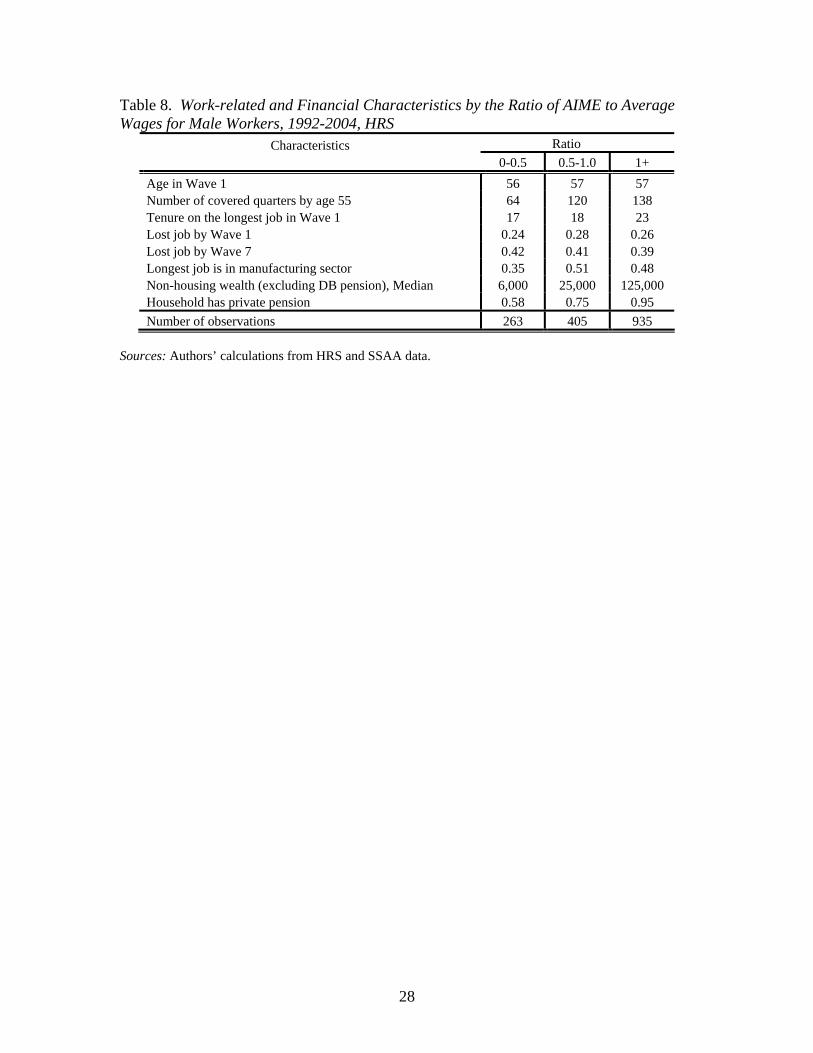
Tables 8 and 9 provide further evidence that the proposed policy would be

effective in protecting those at risk of being adversely affected by an increase in the EEA.

In addition to being much more likely to be in poor health, individuals for whom the EEA

would increase by less than one year are also much less wealthy and less likely to have

private pension coverage. However, it should be acknowledged that AIME is an

imperfect indicator of potential hardship. Some workers who are in poor health or who

would otherwise face difficulty working beyond age 62 would experience an increase in

the EEA under the proposed policy, and some who would continue to qualify for receipt

of benefits at 62 would be at little risk of hardship if their EEA were increased to 64.

The proposed policy would be very effective at sheltering those whose lifetime

earnings generally place them at or below the poverty line. Figure 13 shows the

relationship between the poverty line, which has hovered at about 30 percent of average

earnings, and the 50 percent of average wages threshold for increases in the EEA.

Fiscal Impact and Policy Objectives

Increasing the EEA has very little effect on the finances of the Social Security

retirement benefit program due to the actuarial adjustment made to the benefits of early

claimers. The point of increasing the EEA is to promote benefit adequacy, not to shore

up the system’s finances. However, changes in the EEA are likely to create spillovers

that affect the finances of other public programs.

If the EEA were increased for the low-AIME group rather than held constant, it

would likely put upward pressure on expenditures in other programs. For example,

Figure 14 shows that men in the low-AIME group are much more likely than those in the

high-AIME group to have applied for Disability Insurance (DI) or Supplemental Security

Income (SSI) benefits. Increasing the EEA of workers in the low-AIME group would

exacerbate this pattern, leading to increased expenditures on these and other government

social programs.

17

Holding the EEA constant for the low-AIME group protects the most vulnerable

workers from the hardships associated with delays in benefit eligibility. It also reduces

the fiscal externalities discussed above, but because of the actuarial reduction in benefits

it does so at the cost of reducing the annual benefits accruing to this group after age 64.

This outcome is ironic, because although the low-AIME group profits from a relatively

high replacement rate, they have the lowest absolute level of benefits and retirement

income. So, although they are arguably the group most in need of protection against

inadequate retirement income, which is the whole point of increasing the EEA, they are

the group that would effectively be exempt from the policy change.

It is difficult, or at least expensive, to devise policies that reconcile the objective

of protecting the low-AIME group from potential hardships associated with an increase in

the EEA while simultaneously protecting early claimers from erosion of benefits as the

NRA increases. Applying a less than actuarially fair reduction in benefits to early

claiming by members of the low-AIME group would protect benefit adequacy, but at the

cost of increased program expenditures and the introduction of an economic incentive to

claim benefits early. Making the benefit formula more progressive would get around the

incentive for early claiming problem, but at the potential cost of an even larger increase

in expenditures (unless benefits were reduced for the high-AIME group). Therefore,

policymakers cannot avoid making hard choices in reforming the EEA.

V. Conclusion

As the Normal Retirement Age rises to 67, some have suggested raising the Early

Eligibility Age (EEA) as well. One concern about raising the EEA is that it may create

excessive hardship for unhealthy or worn-out workers by forcing them to continue to

work. The aim of this research is to evaluate alternative policies for a non-uniform

increase in the EEA that addresses this concern.

This analysis first considers a simple rule of increasing the EEA to 64 while still

allowing those with at least 35 years in the labor force to claim reduced benefits that are

actuarially fair. This rule is based on the assumption that lower-educated individuals

usually have more physically-demanding jobs, and thus are more likely to be worn-out or

18

unhealthy. This rule also assumes that these workers would begin their work lives earlier

and thus would have more years in the labor force at a given age.

The HRS Social Security Administrative data provide evidence that this simple

rule does not satisfy our stated goal. In fact, we find a positive correlation between good

health and years in the labor force. As an explanatory variable in the decisions to claim

benefits at 62 and to exit the labor force before age 63, we find that the more years a

worker is in the labor force, the less likely he is to claim benefits and retire early. Thus, it

appears this simple rule for applying an increase in the EEA would not allow most

unhealthy or worn-out individuals the option to claim benefits at 62.

We next evaluate a policy tying an individual’s EEA to a measure similar to the

Average Indexed Monthly Earnings (AIME) calculated by the Social Security

Administration. We provide evidence that low average lifetime wages are correlated

with poor health, a work-limiting condition at age 63, and ever applying for DI or SSI.

This proposed policy has the potential of raising the EEA for most workers without

placing a serious hardship on workers who are worn out or in poor health.

19

References

Burkhauser, Richard V., Kenneth A. Couch, and John W. Phillips. 1996. "Who Takes Early

Social Security Benefits? The Economic and Health Characteristics of Early Beneficiaries." Gerontologist 36 (6): 789-799.

Congressional Budget Office. 1999. Raising the Earliest Eligibility Age for Social Security

Benefits. Washington, DC: U.S. Government Printing Office. French, Eric. 2005. “The Effect of Health, Wealth, and Wages on Labour Supply and Retirement

Behaviour.” Review of Economic Studies 72: 395-427. Gustman, Alan L. and Thomas L. Steinmeier. 2002. “The Social Security Early Entitlement Age

in a Structural Model of Retirement and Wealth.” Working Paper 9183. Cambridge, MA: National Bureau of Economic Research.

Herd, Pamela. 2005. “Ensuring a Minimum: Social Security Reform and Women.” Gerontologist

45: 12-25. Munnell, Alicia H. and Jerilyn Libby. 2007. “Will People Be Healthy Enough to Work Longer.”

Issue in Brief 7-3. Chestnut Hill, MA: Center for Retirement Research at Boston College. Munnell, Alicia H., Kevin B. Meme, Natalia A. Jivan, and Kevin E. Cahill. 2004. “Should We

Raise Social Security’s Earliest Eligibility Age?” Issue in Brief 18. Center for Retirement Research at Boston College.

Panis, Constantijn, Michael Hurd, David Loughran, Julie Zissimopoulos, Steven Haider, and

Patricia St. Clair. 2002. “The Effects of Changing Social Security Administration's Early Entitlement Age and the Normal Retirement Age.” DRU-2903-SSA. RAND.

Steuerle, Eugene C. 2005. “Social Security – A Labor Force Issue.” Statement before the

Subcommittee on Social Security, Committee on Ways and Means, United States House of Representatives. Available at: http://www.urban.org/UploadedPDF/900819_Steuerle_061405.pdf

Steuerle, C. Eugene, Christopher Spiro, and Richard W. Johnson. 1999. “Can Americans Work

Longer?” Straight Talk on Social Security and Retirement Policy 5. Washington, DC: Urban Institute. Available at: http://www.urban.org/url.cfm?ID=309228

Sullivan, Daniel and Till von Wachter. 2006. “Mortality, Mass-Layoffs, and Career Outcomes:

An Analysis using Administrative Data.” Working Paper 2006-21. Chicago, IL: Federal Reserve Bank of Chicago.

Turner, John A. 2007. "Promoting Work: Implications of Raising Social Security's Early

Retirement Age." Work Opportunities Brief 12. Chestnut Hill, MA: Center for Retirement Research at Boston College.

20

University of Michigan. Health and Retirement Study, 1992-2004. Ann Arbor, MI. University of Michigan. Health and Retirement Study, Social Security Administration

Administrative Data, 1951-2003. Ann Arbor, MI. U.S. Census Bureau. 2007. “Poverty Thresholds.” Washington, DC: U.S. Department of

Commerce. Available at http://www.census.gov/hhes/www/poverty/threshld.html. U.S. Social Security Administration. 2000. Government Pension Offset and Windfall Elimination

Provision. Testimony of Jane L. Ross before the Subcommittee on Social Security, Committee on Ways and Means, U.S. House of Representatives. Washington, DC.

U.S. Social Security Administration. 2007. “National Average Wage Index.” Washington, DC.

Available at http://www.ssa.gov/OACT/COLA/AWI.html. Weller, Christian E.2005. “Raising the Retirement Age for Social Security: Implications for Low

Wage, Minority, and Female Workers.” Washington, DC: Center for American Progress. Available at http://www.americanprogress.org/.

White, Joseph. 2006. “Discussions at the National Academy of Social Insurance Annual

Conference.” Washington DC.

21

Table 1. Distribution of Individuals by Claimant Type, 1992-2004, HRS

Worker's benefits: Takers Postponers Spousal benefits: Takers Postponers Other Non-OASI: Ineligibles DI Claimants

Males Females Total Frequency Percent

Frequency

Percent

Frequency

Percent

793 43.64771 42.43

4 0.2210 0.55

443338

306142

30.3423.15

20.969.73

1,236 1,109

310 152

37.7233.84

9.464.64

36 1.98203 11.17

78153

5.3410.48

114 356

3.4810.86

Total

Sources: Authors’ calculaSocial Security Administr

1,817 100 1,460 100 3,277

tions from University of Michigan, Health and Retirement Study (HRS) and ation Administrative (SSAA) data, 1992-2004.

100

22

Table 2. Detailed Distribution by Claimant Type, 1992-2004, HRS

Worker's Benefits: Takers Postponers Spousal benefits: Dual Claimants Takers Dual Claimants Postponers Spousal Only Takers Spousal Only Postponers Other Non-OASI: Ineligibles DI Claimants

Females Total Frequency Percent

Frequency

Percent

443 30.34338 23.15

219 15.0079 5.4187 5.9663 4.32

1,2361,109

223

858767

37.7233.84

6.81 2.59 2.65 2.04

78 5.34153 10.48

114356

3.48 10.86

Total

Sources:

1,460

Authors’ calculations from HRS and SSAA data.

100 3,277 100

23

Total

Men Women

Takers

Postponers Takers

Postponers

793 (34%) 771 (33%) 443 (19%) 338

(14%) Covered quarters at 62: Mean Median Standard deviation Self-reported poor health Self-reported health limitation Physical job Non-Housing wealth: Mean Median Standard deviation DB only (household) DC only (household)

Both DB and DC (household) Less than HS

HS only Some college College degree

143.515534.3

165 (40%) 183 (45%) 123 (26%)

275,68976,000

792,448

188 (44%) 72 (32%)

427 (31%)

194 (38%)

287 (36%) 151 (31%) 161 (29%)

143.915636.3

104 (25%) 89 (22%)

224 (47%)

286,39186,000

738,217

92 (21%) 84 (37%)

493 (36%) 181 (35%)

214 (27%) 143 (29%) 233 (42%)

116.4 120 35.8

99 (24%)

105 (26%) 52 (12%)

365,064 80,500

2,045,737

104 (24%) 32 (14%)

248 (18%)

100 (19%)

167 (21%) 103 (21%)

73 (13%)

116.812035.9

40 (10%) 30 (7%)

77 (16%)

223,61665,250

499,198 47 (11%) 36 (16%)

213 (15%)

41 (8%)

123 (16%)

92 (19%) 82 (15%)

Note: Percentages in parentheses are row percentages.

Sources: Authors’ calculations from HRS and SSAA data.

Table 3. Characteristics of Individuals Claiming Worker Benefits, 1992-2004, HRS

24

Table 4. Characteristics of Individuals Claiming Spousal Benefits, Females only, 1992-2004, HRS

Total

Dual Entitlement Spousal Only

Takers

Postponers Takers

Postponers 219

(49%) 79 (18%) 87 (19%) 63 (14%) Covered quarters at 62: Mean Median Standard deviation Self-reported poor health Self-reported health limitation Physical job Non-Housing wealth: Mean Median Standard deviation DB only (household) DC only (household)

Both DB and DC (household) Less than HS

HS only Some college College degree

64.3

6431.8

38 (40%) 50 (46%) 24 (60%)

394,372133,000

1,780,017 48 (48%) 24 (42%)

114 (58%)

37 (36%) 104

(54%) 58 (58%) 20 (38%)

58.1

5932.6

13 (14%)

9 (8%) 12 (30%)

456,891121,760831,319

15 (15%) 12 (21%)

39 (20%)

11 (11%)

35 (18%) 16 (16%) 17 (32%)

16 13

13.2

27 (28%) 29 (26%)

-

381,069 62,500

857,030

32 (32%) 14 (25%)

13 (7%)

33 (32%)

33 (17%) 17 (17%)

4 (8%)

14.8

1510.5

17 (18%) 21 (19%)

-

209,22691,000

292,541

5 (5%) 7 (12%)

32 (16%)

21 (21%)

21 (11%) 9 (9%)

12 (23%) Note: Percentages in

parentheses are row percentages.


25

Table 5. Labor Force Participation after Claiming OASI Benefits at 62, 1992-2004, HRS

Worker's benefits: Takers stay Takers exit Spousal benefits: Dual Entitlement Takers stay Dual Entitlement Takers exit Spousal Only Takers stay Spousal Only Takers exit

Males Females Frequency Percent

Frequency

Percent

321 40.48472 59.52

1 -3 -- -- -

150293

74

1896

37

33.86 66.14

28.14 71.86 13.95 86.05

Total

Sources:

797 749

Authors’ calculations from HRS and SSAA data.

26

Variable Coefficient (Std. Err.) Equation 1 : Decision to claim early benefits Being in 20-40% of wealth distribution Being in 40-60% of wealth distribution Being in 60-80% of wealth distribution Being in 80-100% of wealth distribution High school graduate Some college College and above Self-reported poor health Number of quarters covered at 63 Both DB and DC DB only DC only Intercept

0.085-0.0940.0260.1910.2240.058

-0.2230.314

-0.0020.0120.528

-0.0740.033

(0.119) (0.119) (0.122) (0.125) (0.091) (0.104) (0.104) (0.091) (0.001) (0.105) (0.121) (0.136) (0.164)

Equation 2 : Decision to exit labor force at or before 62 Being in 20-40 % of wealth distribution Being in 40-60% of wealth distribution Being in 60-80% of wealth distribution Being in 80-100% of wealth distribution High school graduate Some college College and above Self-reported poor health Number of quarters covered at 63 Both DB and DC DB only DC only Intercept


-0.114-0.307-0.0340.1970.12

0.072-0.2760.399

-0.0090.3050.6050.0010.708

(0.121) (0.123) (0.125) (0.128) (0.094) (0.107) (0.109) (0.091) (0.001) (0.112) (0.125) (0.145) (0.166)

Table 6. Estimation Results : Bivariate Probit (Men only), 1992-2004, HRS

27

Table 7: Number of Males Who Claim at Age 62 with Certain Characteristics, by Eligibility to Claim at Age 62 According to the 140 Quarters Rule, 1992-2004, HRS Number of individuals 554

Eligible Not Eligible (69.86%) 239 (30.14%)

Self-reported poor health 99 (60.00%) 66 (40.00%) Self-reported health limitation 103 (56.28%) 80 (43.72%) Continue working (under present rule) 264 (82.24%) 57 (17.76%) In 0-20% of wealth distribution 51 (45.95%) 60 (54.05%) In 20-40% of wealth distribution 107 (66.05%) 55 (33.95%) In 40-60% of wealth distribution 129 (77.71%) 37 (22.29%) In 60-80% of wealth distribution 118 (69.82%) 51 (30.18%) In 80-100% of wealth distribution 149 (80.54%) 36 (19.46%) DB only (household) 122 (64.89%) 66 (35.11%) DC only (household) 53 (73.61%) 19 (26.39%) Both DB and DC (household) 332 (77.75%) 95 (22.25%) Less than high school 117 (60.31%) 77 (39.69%) High school graduate 228 (79.44%) 59 (20.56%) Some college 101 (66.89%) 50 (33.11%) College and above 108 (67.08%) 53 (32.92%) Note: Percentages in parentheses are row percentages.


28

Table 8. Work-related and Financial Characteristics by the Ratio of AIME to Average Wages for Male Workers, 1992-2004, HRS

Characteristics Ratio 0-0.5 0.5-1.0 1+

Age in Wave 1 56 57 57 Number of covered quarters by age 55 64 120 138 Tenure on the longest job in Wave 1 17 18 23 Lost job by Wave 1 0.24 0.28 0.26 Lost job by Wave 7 0.42 0.41 0.39 Longest job is in manufacturing sector 0.35 0.51 0.48 Non-housing wealth (excluding DB pension), Median 6,000 25,000 125,000 Household has private pension 0.58 0.75 0.95 Number of observations 263 405 935


29

Table 9. Characteristics of Affected versus Unaffected Male Workers Claiming Benefits before Age 64, 1992-2004, HRS

Unaffected or Affected by Characteristics affected by less than a more than 1

year year Age in Wave 1 56 56 Less than high school 0.4 0.21 High school 0.27 0.39 Some college 0.17 0.18 College + 0.16 0.21 Poor health at age 63 0.32 0.15 Work limiting health cond. by age 63 0.26 0.19 Spouse has work limiting health cond. by age 63 0.24 0.17 Probability of living till age 75, Median 60 70 Non-housing wealth (excluding DB pension), Median 18,000 110,000 Ever applied for SSI/DI 0.21 0.07 Ratio 0.65 1.28Tenure on the longest job 17 23 Number of covered quarters by age 55 104 138 Number of observations 323 645


30

Source: Authors’ illustration.

HRS

10,560 9,301

Age 63 by 2004

3,807

Information on Social Security

benefit type

3,777

Information on covered quarters

of earnings

3,277

Final Sample

Exclude Widow(er)s and

Caretakers of children under 16

Figure 1. Sample Selection

31

Figure 2. Age Distribution for Worker and Spousal Claimants, 1992-2004, HRS


32

Figure 3. Age Distribution for Worker and Spousal Claimants, by Gender, 1992-2004, HRS


33

Figure 4. Number of Accumulated Quarters by Age and Health Status at Age 63, 1992-2004, HRS

050

010

015

qT

n)ea

m(

20 40 60 80age

Unhealthy Healthy

Note: “Healthy” refers to individuals reporting good, very good, or excellent health. “Unhealthy” refers to individuals reporting fair or poor health. Sources: Authors’ calculations from HRS and SSAA data.

34

Figure 5. Proportion of Unhealthy Individuals by Number of Covered Quarters, 1992-2004, HRS

908070

t 60

cen

re 50

P 4030

20100

Less than 40 40-80 80-120 120-160 160 or more

HealthyUnhealthy


35

Figure 6. Covered Earnings by Health Status at Age 63, 1992-2004, HRS

00

0010

000

200

0030

000

40n

ear

n)ea

m(

20 40 60 80age

Unhealthy Healthy


36

Figure 7. Health-related Obstacles to Work at Age 63 by the Ratio of AIME to Average Wage for Male Workers, 1992-2004, HRS

45

40

35

30

25

rcen

tPe 20

15

10

5

00-0.5 0.5-1.0 1+

Poor/Fair healthHealth cond. limiting workSpouse has health cond. limiting work

Ratio


37

Figure 8. Educational Attainment by the Ratio of AIME to Average Wage for Male Workers, 1992-2004, HRS

50

45

40

35

30

Pe

rcen

t

25

20

15

10

5

00-0.5 0.5-1.0 1.0 +

Ratio

Less than High SchoolHigh SchoolSome CollegeCollege +


38

Figure 9. Self-reported Probability of Living Past Age 75 by the Ratio of AIME to Average Wage for Male Workers, 1992-2004, HRS

80

70

60

50

rcen

t

40

Pe

30

20

10

00-0.5 0.5-1.0 1+

Ratio

Mean Median


39

Figure 10. Proposed Rule: Earliest Eligibility Age (EEA) as a Function of Ratio of AIME to Average Wage in the Economy at Age 55

64.5

64

63.5

63

eA

g

62.5

62

61.5

61

0 0.1 0.2 0.3 0.4 0.5 0.6 0.7 0.8 0.9 1 1.1 1.2 1.3 1.4 1.5 1.6 1.7 1.8 1.9 2

Ratio

EEA

Source: Authors’ illustration.

40

Figure 11. Financial Planning Horizon for Male Workers Age 50-55, 1992, HRS

40

35

30

25

rcen

t

20

Pe

15

10

5

0next few months next year next few years next 5-10 years longer than 10 years

Financial Planning Horizon

Source: Authors’ calculations from HRS.

41

Figure 12. Percent of Male Workers with EEA at Different Ages under Proposed Policy Rule, 1992-2004, HRS

70

60

50

40

rcen

tPe

30

20

10

062 62-64 64

EEA


42

Figure 13. Poverty Threshold and Average Wage Index, 1982-2007

$40,000

$35,000

$30,000

$25,000

$20,000

$15,000

$10,000

$5,000

$0

1982

1983

1984

1985

1986

1987

1988

1989

1990

1991

1992

1993

1994

1995

1996

1997

1998

1999

2000

2001

2002

2003

2004

2005

Year

Poverty Threshold (One person)A.W.I.50 % of A.W.I.

Sources: U.S. Census Bureau (2007) and U.S. Social Security Administration (2007).

43

Figure 14. Percentage of Males Who Ever Applied for SSDI or SSI by the Ratio of AIME to Average Wage in the Economy, 1992-2004, HRS

40

35

30

25

tPe

rcen 20

15

10

5

00-0.5 0.5-1.0 1.0+

Ratio


RECENT WORKING PAPERS FROM THE

CENTER FOR RETIREMENT RESEARCH AT BOSTON COLLEGE

What Makes Retirees Happier: A Gradual or ‘Cold Turkey’ Retirement?

Esteban Calvo, Kelly Haverstick, and Steven A. Sass, October 2007

Why Do Married Men Claim Social Security Benefits So Early? Ignorance,

Caddishness, or Something Else?

Steven A. Sass, Wei Sun, and Anthony Webb, October 2007

Measurement Error in Earnings Data in the Health and Retirement Study

Jesse Bricker and Gary V. Engelhardt, October 2007

Evaluating the Advanced Life Deferred Annuity – An Annuity People Might

Actually Buy

Guan Gong and Anthony Webb, September 2007

Population Aging, Labor Demand, and the Structure of Wages

Margarita Sapozhnikov and Robert K. Triest, September 2007

Work at Older Ages: Is Raising the Early Retirement Age an Option for Social

Security Reform?

John A. Turner, August 2007

The Labor Supply of Older Americans

Alicia H. Munnell and Steven A. Sass, May 2007

Why Do Japanese Workers Remain in the Labor Force So Long?

John B. Williamson and Masa Higo, May 2007

Literacy, Trust and the 401(k) Savings Behavior

Julie R. Agnew, Lisa Szykman, Stephen P. Utkus, and Jean A. Young, May 2007

The Recent Evolution of Pension Funds in the Netherlands: the Trend to Hybrid

DB-DC Plans and Beyond

Eduard H.M. Ponds and Bart van Riel, May 2007

Demographic Influences on Saving-Investment Balances in Developing and

Developed Economies

Ralph C. Bryant, May 2007

All working papers are available on the Center for Retirement Research website

(http://www.bc.edu/crr) and can be requested by e-mail ([email protected]) or phone (617-552-1762).

a new approach to raising social security’s ... -...

Documents