A New Approach to the Feasibility Pump in Mixed Integer

Programming∗

N. L. Boland ‡¶ A. C. Eberhard†§ F. Engineer ‡∗∗ A. Tsoukalas, †∥

26th December, 2011

Abstract

The feasibility pump is a recent, highly successful heuristic for general mixed integer linearprogramming problems. We show that the feasibility pump heuristic can be interpreted as adiscrete version of the proximal point algorithm. In doing so, we extend and generalize some ofthe fundamental results in this area to provide new supporting theory. We show that feasibilitypump algorithms implicitly minimizes a weighted combination of the objective and a term whichpenalizes lack of integrality. This function has many local minima, some of which correspond tofeasible integral solutions; the feasibility pump’s use of random restarts can be viewed as seekingto escape these local minima when they are not feasible integral solutions. This interpretationsuggests alternative ways of incorporating restarts, one of which is the application of cutting planes.Numerical experiments with cutting planes show encouraging results on standard test libraries.

1 Introduction

In spite of the continuous improvement of both commercial and open source solvers, numerous MixedInteger Programming (MIP) problems of practical importance remain intractable. In practice, whererigorous algorithms fail, heuristics often succeed to provide feasible solutions of good quality. Apartfrom their self evident value, good feasible solutions are also useful in speeding up the search of branchand cut algorithms. General purpose heuristics include [2, 3, 4, 13, 14, 15, 16, 19, 20, 21, 22, 23]. Wedirect the reader to [6] for a recent survey.

A heuristic that has attracted significant interest in recent years is the Feasibility Pump(FP) [17].The FP starts from the Linear Program (LP) optimum and computes two trajectories of points, oneinteger and the other LP feasible, by iteratively applying rounding and projection operations. EveryLP-feasible point is rounded to an integer point and every integer point is projected back onto theLP feasible region using the l1 norm. As both the rounding and the projection are minimal distanceoperations (with respect to the l1 norm), the distance between pairs of points on the two trajectoriesdecreases monotonically until the method cycles, unable to further decrease the distance. If the distanceis reduced to zero before cycling then a feasible point has been obtained. Otherwise a random moveis used to restart the method from a new point. In the original FP [17], the only bias of the methodtowards points of good objective value is the starting point, so the random restarts threaten to escapethe good quality area. Thus, the feasibility pump uses a sophisticated restart scheme, attemptingto displace the current point in an economic way by “minor perturbations”, and performs a “majorrestart” only in the presence of further failures.

The FP method demonstrates encouraging performance on a large class of test problems, but behavesbetter for binary problems than for general integer variables. Thus, [5] first deal with the binaryvariables in isolation, treating general integers as continuous variables. General integer variables are

∗This research was supported by the ARC Discovery grant no. DP0987445‡Faculty of Science and Information Technology, School of Mathematical and Physical Sciences,University of Newcastle,

University Drive, Callaghan NSW 2308 Australia†School of Mathematical and Geospatial Sciences, RMIT, GPO Box 2476V, Melbourne, Victoria, Australia 3001.¶Natashia.Boland@newcastle.edu.au§andy.eb@rmit.edu.au

∗∗Faramroze.Engineer@newcastle.edu.au∥angelos.tsoukalas@rmit.edu.au

1

treated as integer in a subsequent second round only after a point satisfying integrality for all binaryvariables is obtained. In [1] the Objective Feasibility Pump (OFP) is proposed, where the projectionproblem is modified to include an objective function term, while in [18] simple rounding is substitutedby a sophisticated constraint propagation approach. The latter makes use of information about the LPfeasible region, with rounding done one variable at a time, while exploiting constraint information todisqualify unacceptable values. A modified penalty function is used in [27] that implicitly promotes abias towards fixing more variables at integral values during the projection step.

The numerical results presented in [1] indicate that adding an objective term to the projectionproblem is beneficial to the quality of the solution, while not compromising computation time toomuch. Constraint propagation [18] is shown to further improve solution quality while also decreasingthe failure rate of the method. The modified penalty function of [27] yields an improvement in efficiencyand number of iterations relative to the original FP [17]. Recently the FP has been successfully extendedto nonlinear problems, see for example [8, 10, 11], which focus on the challenge introduced by nonlinear(and nonconvex) constraints.

In this paper, we explore the relationship between generalized forms of the FP and proximal pointalgorithms, in the context of linearly constraint (possibly nonlinear) integer programs (see, for example,[9, 26]). In doing so, we provide insights about the properties of the points generated by the FP method,and of its mathematical behaviour. Aside from the OFP, methods that improve the original FP can becharacterized as either putting some of the LP into the rounding step (e.g. constraint propagation in[18]), or putting some integrality into the projection step ([27]). Here we also propose to explore thelatter, but in a different way: by incorporating integer cutting planes into the LP projection step.

We consider the general nonlinear MIP

min g(x)

s.t. Ax ≥ b, xI ∈ I, (1)

where g : Rn → R is a possibly nonlinear continuous function, I is the index set of integer variables,and I = Zm, where m = |I|. The remaining variables, denoted by xR, are allowed to vary overRn−m; the nonlinear MIP feasible set is F := {x ∈ Rn | Ax ≥ b, xI ∈ I}. We will refer to integralpoints as being those points x ∈ Rn for which xI ∈ I. Although the objective may be nonlinear,throughout we will refer to the feasible set with integrality relaxed as the LP feasible set, defined asFLP := {x ∈ Rn | Ax ≥ b}.

In this paper we will show that the FP heuristic can be interpreted as a kind of proximal pointmethod, by comparing the FP with the primal-proximal heuristic introduced in [12]. Our analysisfocusses on the “inner loop” of the FP method, during which the two trajectories of rounded andprojected points are calculated, before cycling necessitates a perturbation or restart. We call this thepumping process, and the points generated by rounding during this process the discrete proximal pointiterates. Each of these points is associated with the LP feasible point it was rounded from: we call thesethe LP-feasible iterates. The key departure of the FP method from standard proximal point methodsis the rounding step, which in effect is a projection onto the integer points, giving a point minimizingI(x) := min {∥xI − yI∥1 | yI ∈ I}. Thus the rounding step implicitly calculates the measure of lackof integrality given by I(x), where x is an LP-feasible iterate. One of the important results of ouranalysis in this paper is that LP-feasible iterates generated during the pumping process converge to alocal minimum of the function g+ rI on FLP , where r > 0 is a parameter that weights the importanceof the two conflicting objectives. Thus local minimization of the objective g+rI over FLP is associatedwith cycling events in the FP method.

In [24] and [27] pure Integer Programs (IP) were studied and it was noted that the global minimizersof various penalized continuous problems over FLP coincide with the global optimal solutions of theoriginal IP. In this paper we will show that a similar interpretation of the original FP [17] and theObjective Feasibility Pump (OFP) [1] can be made for a Mixed IP (MIP). Thus if the pumping processof an FP method can be started in the right region, (and with the right value for the parameter r), itwill converge to an optimal solution of the MIP. Interestingly, FP methods do contain a mechanism forre-starting the pumping process.

When the FP method detects cycling it performs either a “major” or “minor” restart, both usingsome form of randomization. These restarts form the outer loop of iterates of the FP. We providenumerical results which show that the repeated use of major restarts in particular correlates well withcases in which poorer solution quality is obtained by the FP method. Our analysis explains that

2

cycling occurs because local optimality of the function g + rI over FLP has been obtained, and hencesuggests some alternative ways to overcome this problem when this local minimum is not integral.Two approaches to escaping these undesirable local optimum present themselves: effect a change oneither the objective function or the feasible region FLP . The former can be achieved by varying theweighting parameter r > 0; we plan to consider this approach in future work. In this paper, we focuson the latter, and propose to alter the feasible region via the introduction of cuts to remove the local,non-integral minimum at which the cycling has occurred. We give encouraging numerical experimentswhich demonstrate the potential for this cutting strategy. We show the strategy tends to delay the useof major restarts, and leads to improvements in the quality of the feasible integral solutions found.

The paper is structured as follows. In Section 2 we reinterpret the inner iterates of the FP as a kindof a proximal point iteration and discuss the connection this interpretation has to the primal-proximalheuristic introduced in [12]. As we require more general versions of some results of [12, sections 1.3 and2] we provide extensions of these results for our nonlinear MIP in Section 3. In particular, we showthat quite general coercive penalties can be used in place of the l2 norm which was used in [12] in orderto exploit Lagrangian relaxation techniques. As the FP exploits LP relaxations our analysis departsfrom that of [12] significantly at this point and in Section 4 we complete the development begun inSection 2 by showing how the minimization of g+rI over FLP results from such proximal point iterates(the “pumping process”). In Section 5 cycling is shown to be associated with the failure to locate anintegral LP feasible point at a local minimum of g+ rI. A modification of the OFP algorithm of [18] isproposed in Section 6. Here extensive numerical testing is undertaken in which we selectively introducecuts to prevent cycling instead of the sole use of minor perturbations.

2 FP, Proximal Points and Concave Penalties

In this section we draw out some comparisons and contrasts with recent approaches that convertinteger programs to nonlinear continuous optimization problems. Consider the general nonlinear MIP(1). Proximal point approaches [12] consider regularising this problem using a penalty ρ (x) to obtaina continuous optimization problem

miny

φr (y) where (2)

φr (y) :=min {g (x) + rρ (x− y) | x ∈ F} . (3)

Regularization is a common tool used in nonlinear and nonsmooth optimization. In a sense, MIPs arehighly nonsmooth, as their domains are disconnected. Regularization in the form of (3) can be seen as amathematical tool to construct, in a systematic way, an equivalent continuous problems, with smootherfunctions. The results can have attractive properties, as we will see in Section 3 and Section 4.

The analysis of the problem (2) when ρ is the Euclidean l2 norm was carried out in some detail in[12]. The main property that arises is that integrality of local minima of (2) is assured and do oftencorrespond to the feasible solutions of (1). Indeed y0 (where (y0)I ∈ I) is a local minimum of φr exactlywhen x = y0 is the solution to the minimization problem φr(y0).

Since the calculation of the objective φr is as difficult as the original MIP, in [12] Lagrangian relax-ation is used to obtain a solvable relaxed problem. This gives an underestimate φr of φr. Unfortunatelythe local minima of the relaxation φr are not assured to be integral. In Section 3 of [12], approachesto varying the parameter r > 0 to obtain feasible integral points are considered, but the results areinconclusive and the tone of [12] is quite negative in this respect. In the final section of [12] binaryproblems are addressed and a penalty used to enforce integrality, but no role for rounding is considered.

The OFP, by contrast, drops the integrality constraint in (3) and takes ρ to be an l1 norm, so thata relaxation of φr when g (x) = cTx can be calculated as a linear program. Thus we arrive at theproblem

miny

φLPr (y) where (4)

φLPr (y) :=min {g (x) + r ∥x− y∥1 | x ∈ FLP } . (5)

Proximal point algorithms seek local optima by a kind of fixed point iteration, where the center y isreplaced at each step by the optimal solution of the regularization problem (e.g. of (5)). FP methodsalso take this approach, but to try and encourage integrality of a solution, a new center at y0 with

3

(y0)I ∈ I is sought at each iterate. If x = y0 is the solution to the minimization problem, the FP methodis clearly finished, having obtained a feasible integral point. Otherwise, the non-integral solution of (5)is rounded to the nearest integral point in order to provide the new center for the next iteration.

Since FP methods use the l1 norm, the analysis of [12] does not directly apply. Thus in order toestablish similar properties, we in Section 3 extend these results, and in doing so, prove they hold forgeneral class of coercive functions ρ, including the l1 norm as a special case. This allows us to showthat regularisation preserves the global minimizers (which are the optimal solutions of the MIP) andretains the same local minimizers (which correspond to the feasible integrals solutions of the MIP).These correspondences are established in Section 3 for our general nonlinear MIP.

In Section 5 we show that the pumping process applied in an OFP setting finds local optima of g+rIover FLP and so the function I acts as a penalty for the deviation from integrality. The original FP isessentially the limiting version of the scheme for r →∞. Thus the pumping phase of the FP implicitlyperforms a minimization of a concave nonlinear integrality penalty via a combination of projective LPsand roundings. Our results provide some additional insights. For example, if the OFP finishes earlywithout major restarts, it appears likely that the resulting solution will be both an optimal for theoriginal MIP and a global minimum of g + rI.

This approach is distinct from that proposed in [24] where piecewise concave penalties are usedto obtain an exact penalization for IPs and is motivated by the long observed connection that binaryprograms have to concave minimization. This is exploited in [27] to provide an interpretation of theFP for the case of binary problems. Motivated by the observation of [14] they note that the originalFP [17] for binary problems can be interpreted as a Frank-Wolfe method [7, Section 2.2.2] as appliedto a non-differentiable concave function over the feasible set FLP . They develop theory that relates theglobal minima of these continuous penalized problems to the solution of an IP. We are able to providesimilar results in Section 5 thus showing a connection of our approach to that used in [24].

3 General Properties of Regularizations

In this section we generalise key results of [12]. The generalisation takes two forms: we use a generalclass of coercive penalty ρ instead of ρ = ∥·∥2, and give results for Mixed rather than pure IPs. Thisyields results for ρ = ∥·∥1 that apply to the FP heuristic for MIPs. In particular, we show that theregularization (2) has global and local minimizers closely related to the optimal and feasible points ofthe original MIP. We posit the following assumptions.

Assume: A continuous function ρ : Rn → R that satisfies the following conditions is called aninteger compatible regularization function (ICRF) iff:

Condition 1 ρ (x) ≥ 0 for all x and x = 0 iff ρ (x) = 0.

Condition 2 If γ ∈ (0, 1) then ρ (γx) < ρ (x) for all x = 0.

Condition 3 There exists a continuous, strictly increasing, function s (·) : R+ → R+ and a K such that for allK < K we have ρ (x) ≤ K implies ∥x∥1 ≤ s−1(K) for the l1 norm ∥·∥1 on Rn.

Remark 1 These properties are deliberately chosen to be general enough to allow all of the theory tocover the case of any norm on Rn and for most of the theory to encompass the cases of some concavepenalties already introduced in the literature for binary problems. Recall that in finite dimensions allnorms are equivalent to the l1 norm i.e. for all norms ∥·∥ there exists constants A,B > 0 such thatA ∥·∥1 ≥ ∥·∥ ≥ B ∥·∥1. With this in mind it is clear how these assumptions relate to equivalent norms.

In [27] and [24] penalty functions were generated as follows:

ρ (x) :=∑i

p (|xi|) (6)

where p : R+→ R+ is a concave, strictly increasing function. Some examples taken from [27] that were

4

used explicitly for binary problems are:

p (t) = log (t+ α)− logα, (7)

p (t) = −[t+ α]−q + α−q, (8)

p (t) = 1− exp (−αt) , (9)

p (t) = [1 + exp (−αt)]−1 − 1

2, (10)

for some α, q > 0. We wish to include these functions in our analysis in order to make some comparisonswith the approaches in [27] and [24]. It is interesting to note that the case when p(x) = x correspondsto p being both simultaneously concave and convex and to ρ(·) = ∥ · ∥1.

The following justifies the use of the conditions 1 to 3 above for penalties of the form (6).

Proposition 2 Suppose ρ is defined via (6) with p (0) = 0, p (t) > 0 for t = 0 and p concave, lowersemi-continuous and strictly increasing function. Then ρ is an integer compatible regularization func-tion. In particular when the Range p = [0,+∞) we may take K = +∞.

Proof. Suppose

ρ (x) =∑i

p (|xi|) ≤ K

then for each i we have |xi| ≤ p−1(K) when K ∈ Range p. As Range p contains an interval of the type[0, b) we may take 0 < K < K := b. In particular when b = +∞ we can take K = +∞. Consequently

∥x∥1 ≤√n ∥x∥∞ ≤

√np−1(K)

and hence ρ satisfies Condition 3 with s(·) := 1√np(·). Clearly ρ ≥ 0 and ρ (x) = 0 iff ∥x∥1 = 0. As s is

strictly increasing ρ (γx) =∑

i p (γ |xi|) <∑

i p (|xi|) = ρ (x).

Let

f (x) :=

{g (x) if Ax ≥ b, xI ∈ I+∞ otherwise

,

where g : Rm → R is a continuous function. Then

φr (y) = inf {g (x) + rρ (x− y) | Ax ≥ b, xI ∈ I}= inf {f (x) + rρ (x− y) | x ∈ Rn} .

Definefr (x, y0) := f (x) + rρ (x− y0) for all x ∈ Rn

and so φr (y0) = inf {fr (x, y0) | x ∈ Rn}. Note that as g is continuous and the feasible region F :={x | Ax ≥ b, xI ∈ I} is a closed set it follows that f : Rm → R is a lower semi-continuous function.We also observe that as φr is an infimum of a family of continuous functions y 7→ f(x) + rρ(x − y)it is, at worst, an upper semi-continuous function of the variable y. We can claim more under mildconditions. Denote the epigraph epi f := {(x, α) | f(x) ≤ α} and note that epih ⊇ epi f + epi rρ if andonly if h(y) ≤ f(x) + rρ(x− y) for all x, y ∈ Rn. Thus geometrically epiφr is the largest extended realvalued function whose epigraph contains the sum epi f + epi rρ.

Theorem 3 Suppose g : Rn → R is continuous and the feasible region F is closed and nonempty.Suppose in addition that the regularized function φr(y0) > −∞ for some y0 and that ρ is a ICRF thatis also Lipschitz continuous (with a global Lipschitz constant). Then φr is a finite valued for r ≥ r andglobally Lipschitz continuous.

Proof. Clearly φr(y) ≥ φr(y) for all y and r ≥ r. Thus when φr(y) > −∞ for all y then φr(y) > −∞for all r ≥ r. Moreover as φr(y) ≤ g(x) + rρ(x− y) < +∞ for any x ∈ F finiteness of φr follows. Thusif we can show φr(y) is bounded away from negative infinity for all y then we would have shown it tobe finite valued.

Let Cµ denote the cone epiµ∥ · ∥. Note next that the Lipschitz continuity property of ρ correspondsto the existence of a Lipschitz constant µ > 0 such that epi ρ + Cµ ⊆ epi ρ. Now epi ρ + Cµ ⊆ epi ρ inturn implies epi rρ+ Crµ ⊆ epi rρ with intCrµ = ∅ for all r.

5

Suppose φr(y) = −∞ for some y then

(y,−n) ∈ epi f + epi rρ

for all n ∈ Z+ and so (using intCrµ = ∅)

Rn+1 ⊆∞∪

n=1

((y,−n) + Crµ) ⊆ (epi f + epi rρ) + Crµ

⊆ epi f + (epi rρ+ Crµ) ⊆ epi f + epi rρ ⊆ epiφr

implying φr ≡ −∞, contradicting φr(y0) finite. Let φr(y) < α and take x such that f(x)+rρ(x−y) < α.Let z ∈ Rn then

φr(z) ≤ f(x) + rρ(x− z) ≤ (f(x) + rρ(x− y)) + r (ρ(x− z)− ρ(x− y))

< α+ r (ρ(x− z)− ρ(x− y)) ≤ α+ rµ∥z − y∥,

where we have used the Lipschitz continuity of ρ again. As this holds for all α > φr(y) we haveφr(z) ≤ φr(y) + rµ∥z − y∥. As y, z ∈ Rn are arbitrary we are finished.

Remark 4 The conditions of Theorem 3 are satisfied for any norm and all the concave penalties formedvia (6) using the various choices for the function p.

The following results are a generalization of the results of [12] Section 1 and these form a basictool in the proof of subsequent properties. The most important property is Property 3 which roughlysays that local minima of φr are not only integral but correspond to “fixed points” of the mappingy0 7→ argmin {fr (x, y0) | x ∈ Rn}.

Lemma 5 Posit the assumption that ρ is an ICRF.

1. For all y ∈ Rn the function r 7→ φr (y) is nondecreasing.

2. φr (y) ≤ f (y) for all y ∈ Rn for all r ≥ 0.

3. Assume f is bounded from below. Then there exists r > 0 such that if y0 is a local minimum ofφr for some r < r then x = y0 is the unique minimum point of fr(·, y0) in

φr (y0) = inf {fr (x, y0) | x ∈ Rn} . (11)

In particular φr (y0) = f (y0) and y0 is integral. Moreover if K = +∞ in the definition of ICRFthen r = 0.

4. Local minima of φr are also local minima of φr′ for r′ ≥ r.

Proof. We show part 3 only, as it is the critical observation; the other observations follow in asimilar way to the results of [12] Section 1. As f is lower semi-continuous and bounded from belowand Condition 3 of the definition of a integer compatible regularization function holds, implying theexistence of function s, we have

{x | g (x) + rρ (x− y0) ≤ K, Ax ≥ a, xI ∈ I} (12)

⊆{x | min

xf (x) + rρ (x− y0) ≤ K

}⊆

{x | ∥x− y0∥1 ≤ s−1

(K −minx f (x)

r

)}which is bounded and nonempty for any K > minx f (x) and r > 0 sufficiently large so that(

K −minx f (x)

r

)< K.

Let y0 be a local minimum of φr, so there exists an integral point x0 ∈ F and a neighbourhood ofy0 denoted by Bε (y0) (for some ε > 0) such that

f (x0) + rρ (x0 − y0) = φr (y0) ≤ φr (y) ≤ f (x0) + rρ (x0 − y)

6

for any y ∈ Bε (y0). Hence ρ (x0 − y0) ≤ ρ (x0 − y) for any y ∈ Bε (y0). Assume that ρ(x0 − y0) > 0.Take y = y0 + t (x0 − y0) and so if x0 − y0 = 0 we have for t sufficiently small

ρ (x0 − y0) ≤ ρ (x0 − y) = ρ ((1− t) (x0 − y0)) < ρ (x0 − y0)

which is a contradiction when 0 < t < 1 under Condition 3 if ρ (x0 − y0) > 0. Thus ρ (x0 − y0) = 0and so x0 = y0 and (y0)I ∈ I with φr (y0) = fr (y0, y0) = f (y0).

The relationship between infy∈Rn φr (y) and inf {g (x) | Ax ≥ b, xI ∈ I} is developed in the nextresult which is essentially Theorem 1.5 of [12] and provided for completeness. This result demonstratesthat there is a direct correspondence between the local and global minimizers of the nonlinear MIP andthe unconstrained continuous regularized problem φr.

Theorem 6 Posit the assumption that ρ is an ICRF. Then the minimization of f and φr are relatedas follows:

1. inf {g (x) | Ax ≥ b, xI ∈ I} = inf {φr (y) | y ∈ Rn} ,

2. if x∗ ∈ argmin {f (y) | y ∈ Rn} = argmin {g (x) | Ax ≥ b, xI ∈ I},then x∗ ∈ argmin {φr (y) | y ∈ Rn} and

3. Suppose r is as specified in Lemma 5 part 3 and f is bounded below. Then for r > r we have y∗

minimizes (resp. locally minimizes) φr then y∗ minimizes (resp. locally minimizes) f .

Proof. Consider the first part. For any x and y in Rn we have fr (x, y) ≥ f (x) and hence φr (y) ≥ inf fand so inf φr ≥ inf f . On the other hand Lemma 5 part 2 gives inf φr ≤ inf f and equality. Supposex∗ ∈ argmin {f (x) | x ∈ Rn}. Then using Lemma 5 part 2 again we have inf φr = inf f = f (x∗) ≥φr (x

∗) and so x∗ ∈ argmin {φr (y) | y ∈ Rn}. Finally, posit the assumption of Lemma 5 part 3 andsuppose y∗ minimizes (resp. locally minimizes) φr then f (y∗) = φr (y

∗) ≤ φr (y) ≤ f (y) for all y (yclose to y0).

The converse of Lemma 5 part 3 may be developed and this result establishes when the localminimizers of the regularized problem are actually strict local minimizers. As the results of this paperare in the main based only on the implication given in Lemma 5 part 3 we relegate the proof of thenext result to an appendix.

Proposition 7 Suppose g is bounded below on the feasible region F , ρ is an ICRF and r > r (asspecified in Lemma 5 part 3). A point y0 is a local minimum of φr if and only if x = y0 with xI ∈ I isa unique optimal solution of

φr (y0) = min {g (x) + rρ (x− y0) | Ax ≥ b, xI ∈ I} . (13)

Indeed if y0 is a local minima of φr then it is a strict local minimum of φr in the following cases.

1. We have an IP (i.e. m = n).

2. (y0)R is a strict local minimum of the continuous partial regularization

Gr (yR) := minzR∈Rn−m

{Gy0 (zR) + rρ (zR − yR)}

of the function Gy0 (zR) := f ((y0)I , zR) : Rn−m → R.

In general we can only assert that when y0 is a local minimum of φr then (y0)R must be a localminimum of Gr while (y0)I is always a strict local minimum of xI 7→ φr(xI , (y0)R).

The next result completes our goal of relating the local minimizers of φr to the feasible solution ofthe MIP defined in (1) and the global minimizers of the regularized problem φr to the global minimizersof the original non-linear MIP defined in (1). This is a generalization of Theorem 2.2 of [12].

Theorem 8 Suppose ρ is an ICRF. Then there exists an r > 0 such that for r > r any local minimumof φr lies in the feasible region F . Moreover

7

1. For r > r large enough, the local minima of φr are exactly the points of F .

2. Suppose that Range ρ = [0,+∞) (and so we may take r = 0). Then for r > 0 small enough, thelocal minima of φr are exactly the optimal solutions of

min {g (x) | Ax ≥ b, xI ∈ I} (14)

in the following cases:

(a) we have m = n i.e. a pure IP, or

(b) both g and ρ are convex functions.

Proof. Consider the first part. In view Lemma 5 part 3 we only need show that if y0 ∈ F then y0 is alocal minimum of φr for r sufficiently large. Consider K := φr (y0) + 2, r > r sufficiently large so thatvia (12) we have the set

FK (y0) := {x ∈ Rm | {f (x) + rρ (x− y0)} ≤ K } (15)

bounded. As f is lower semi-continuous and rg(· − y0) is continuous their sum is also lower semi-continuous implying FK(y0) is a closed set. Next note that as φr(y) is defined as an infimum ofcontinuous functions y 7→ f(x)+rρ(x−y) it is upper semi-continuous. Thus we may take y sufficientlyclose to y0 so that φr (y) + 1 < φr (y0) + 2 := K and for all x ∈ FK (y0) with xI = (y0)I then

ρ (x− y) = ρ (x− y0) + [ρ (x− y)− ρ (x− y0)]

≥ inf {ρ (x− y0) | x ∈ FK (y0) with xI = (y0)I}− [ρ (x− y0)− ρ (x− y)]

= ϵ− [ρ (x− y0)− ρ (x− y)] > 0

where inf {ρ (x− y0) | x ∈ FK (y0) with xI = (y0)I} := ϵ > 0. Take r > 0 sufficiently large so thatϵ2 > Γ

r > 0 where

Γ := max {f (x)− f (x′) | x, x′ ∈ FK (y0)} = max{g(x)− g(x′) | x, x′ ∈ F ∩ FK(y0)},

which is finite as g is continuous, FK (y0) is compact and F is closed. We will assume we take ysufficiently close to y0 so that at least [ρ (x− y0)− ρ (x− y)] < ϵ

2 and hence ρ (x− y) ≥ ϵ2 > Γ

r .Then for x ∈ FK (y0) with xI = (y0)I we have (as y0 ∈ FK (y0))

f (x) + rρ (y − x) = {f (x)− f (y0) + rρ (x− y)}+ f (y0)

≥ −Γ + rϵ

2+ f (y0) ≥ −Γ + r

Γ

r+ f (y0) = f (y0) ≥ φr (y0) .

Next note that if x ∈ FK−1 (y) and we have y is sufficiently close to y0 so that r|ρ (x− y)−ρ (x− y0) | ≤1 then

K − 1 ≥ f (x) + rρ (x− y)

= f (x) + rρ (x− y0) + r (ρ (x− y)− ρ (x− y0))

≥ f (x) + rρ (x− y0)− 1

and so FK−1 (y) ⊆ FK (y0). Consequently

φr (y) = inf {f (x) + rρ (y − x) | x ∈ FK−1 (y)}≥ φr (y0) .

For the second part 2 we argue again along the lines of Theorem 2.2 of [12]. Let y0 be a localminimizer of φr and we already know that y0 ∈ F and that φr (y0) = f (y0) and need to show that y0 isoptimal for the MIP for r small. Denote V ∗ the optimal solutions of the MIP. Place V ∗

I := {xI | x ∈ V ∗},

v+ = min {f (x) | x ∈ F ∩ {x | xI /∈ V ∗I }} and

v∗ = min {f (x) | x ∈ F} .

8

Now as the variables are partly integral valued we have v+ > v∗ as xI = yI if y ∈ V ∗ and xI ∈ V ∗I .

Let K = v∗ + 1 and suppose contrary to assertion that y0 /∈ V ∗ for any r > 0. Denote

D := max {ρ (x− y0) | xI = (y0)I , x ∈ V ∗} .

When D = 0 we immediately have (y0)I ∈ V ∗I . Otherwise D > 0, then we choose 0 < r < (v+ − v∗) /D

and we have for any x∗ ∈ V ∗

f (y0) = φr (y0) ≤ f (x∗) + rρ (x∗ − y0)

≤ f (x∗) + rD < f (x∗) + v+ − v∗ = v+.

As f (y0) < v+ we must have (y0)I ∈ V ∗I once again. If n = m (i.e. we have a IP) we are finished as

then y0 ∈ V ∗.In the final case we assume contrary to theorem that (y0)R /∈ V ∗

R and v∗ < f ((y0)I , (y0)R) =f (y0). As (y0)I ∈ V ∗

I , y0 ∈ F and y0 /∈ V ∗ we must have the existence yR such that ((y0)I , yR) ∈ Fand v∗ = f ((y0)I , yR) < f ((y0)I , (y0)R) . Thus by Lemma 5 part 3 we have

φr ((y0)I , yR) ≤ f ((y0)I , yR)

< f ((y0)I , (y0)R) = miny{f (y) + r (y − y0)} = φr (y0) .

For t sufficiently small we have (1 − t)y0 + t ((y0)I , yR) in the neighborhood in which y0 is the localminimum of φr. When ρ and g are convex we have φr convex and so

φr ((1− t)y0 + t ((y0)I , yR) ) ≤ (1− t)φr (y0 ) + tφr ((y0)I , yR)

< (1− t)φr (y0 ) + tφr (y0) = φr (y0)

implying y0 is not a local minimum of φr, a contradiction.

4 The Proximal Point Heuristic and Relaxation of Integrality

The relationship of the analysis above to FP methods lies in the observation that an OFP iterationsolves (5), i.e. solves the LP relaxation of problem (11) with g (x) = cTx, and the integer compatibleregularization function given by ρ (x) = ∥x∥1. At this juncture it is important to note that Range ρ =[0,+∞) so we may take r = 0, which will be the case for the remainder of the paper unless otherwiseindicated. Recall the definition of φLP

r from (5) and observe that

φLPr (y) ≤ φr (y) (16)

for all y. When g (x) = cTx the problem of calculating φLPr (y) may be reformulated as an LP. Indeed

this is the basis of the FP strategy. Calculating φLPr (y) is not so easy when g is nonlinear, but we carry

out the following analysis without any linearity assumptions on g, and this allows for the possibility ofdeveloping some other novel numerical method in the future.

Remark 9 The analysis of this section (and the next) can be carried out using a much more generalform of an integer compatible regularization function ρ than the l1 norm. In particular, a general norm,or any other convex, integer compatible regularization function, would suffice. For example, if g werequadratic, one could use ρ (x) = ∥x∥2 and then φLP

r (y) could be solved as a quadratic program. As wewish to emphasis our comparison with the feasibility pump, these generalisations are not pursued here.

Placing

h (x) :=

{g (x) if Ax ≥ b, x ∈ Rn

+∞ otherwise

we may write φLPr as a proximal point problem:

φLPr (y0) := inf

x{h (x) + r ∥x− y0∥1} (17)

which is well known to define a convex, Lipschitz function of y0 when g is convex (see [12, Theorem 1.6]and references). The same proof technique as used in Lemma 5 shows that if y0 is a local minimum of

9

φLPr then x = y0 is the unique minimum point of h (·) + rρ ∥· − y0∥1. Now in the event that (y0)I ∈ I

then clearly φLPr (y0) = φr (y0) and x = y0 is the unique minimum point of h (·) + rρ ∥· − y0∥1 over x

constrained to xI ∈ I. Furthermore using (16) and the fact that y0 is a local minimum of φLPr we have

φr (y0) = φLPr (y0) ≤ φLP

r (y) ≤ φr (y) for all y close to y0. (18)

Thus y0 must also be a local minimum of φr. By Theorem 8 we have y0 ∈ {Ax ≥ b, xI ∈ I} andmoreover if g is convex and r is sufficiently small y0 is actually optimal for (14). The OFP [1] increasesr at each step of the pumping process and so between major restarts the magnitude of r is directlyrelated to the iteration number in this pumping process. When the OFP terminates early, without anyrestarts, r will be smaller than it would be if multiple restarts occurred (long durations of the pumpingprocess are not observed in numerical tests). As smaller values of r are needed for the FP to generateoptimal solutions the likelihood that the FP generates an optimal point will be higher when we havefewer restarts.

Proposition 7 indicates that we can detect in (y0)I ∈ I a local minimizer of φr by checking ifxI = (y0)I (∈ I) is a unique optimal solution of (13) or in our case it suffices to check if xI = (y0)I(∈ I)is a unique optimal solution of (17) (for any fixed r > 0 = r). Now when y0 ∈ F := {Ax ≥ b, xI ∈ I}we have from Theorem 8 that y0 is a local minimum of φr for r sufficiently large and hence x = y0is the unique optimal solution of (13). Is the same true for our relaxation (17)? The following partlyanswers this question.

Theorem 10 Assume g is continuous and bounded below on {Ax ≥ b, x ∈ I}.

1. Suppose r is sufficiently small and y0 with (y0)I ∈ I is a local minima of φLPr . Then y0 is an

optimal solution of (14). In particular x = y0 with (y0)I ∈ I is the minimum of the problem

inf {g (x) + r ∥x− y0∥1 | Ax ≥ b, x ∈ Rn} . (19)

2. Suppose r is sufficiently large and y0 with (y0)I ∈ I is a local minima of φLPr . Then y0 ∈ F :=

{Ax ≥ b, xI ∈ I} and x = y0 solves the problem (19). Conversely, when g is convex and y0 ∈ Fthen x = y0 with xI ∈ I solves the problem (19) for r sufficiently large.

Proof. Suppose y0 with (y0)I ∈ I is a local minima of φLPr then by (18) we have y0 a local minimum

of φr and we may now apply Theorem 8 to obtain all but the last assertion.Let y0 ∈ F and as h is convex, lower-semi-continuous and bounded below with domh = {Ax ≥ b, x ∈ Rn}

we may take z0 ∈ ∂h (y0) = ∅. Then for all x ∈ domh we have

h (x)− h (y0) ≥ ⟨z0, x− y0⟩implying g (x) + r ∥x− y0∥1 ≥ g (y0) + r ∥x− y0∥1 − ∥z0∥∞ ∥x− y0∥1

or g (x) + r ∥x− y0∥1 ≥ g (y0) + (r − ∥z0∥∞) ∥x− y0∥1 > g (y0)

for all x ∈ {Ax ≥ b, x ∈ Rn} and all x = y0 when r > ∥z0∥∞. Thus x = y0 with (y0)I ∈ I is the localminimum in (19).

One can of course directly test if a point y0 is feasible but if this test fails how can we improve ournext test point? This is where the above comes into play. Suppose that we start with an initial feasiblepoint x0 ∈ FLP . Denote by y0 ∈ argmin {∥x0 − y∥1 | yI ∈ I} the closest integral point. We solve (19)to obtain x1 ∈ argmin {g (x) + r ∥x− y0∥1 | Ax ≥ b, x ∈ Rn} and find that if x1 = y0 then y0 fails tobe a local minimum of φLP

r . Then when x0 = x1 we have

g (x1) + r ∥x1 − y0∥1 ≤ g (x0) + r ∥x0 − y0∥1 (20)

or g (x1) ≤ g (x0)− r [∥x1 − y0∥1 − ∥x0 − y0∥1] < g (x0) (21)

a decrease in objective value as long as

∥x1 − y0∥1 > ∥x0 − y0∥1 = I (x0)

:= min {∥x0 − y∥1 | yI ∈ I} = ∥(x0)I − (y0)I∥1 . (22)

10

Inequality (21) indicates that this process does not cycle when (22) holds. Using (20), the fact thatI (x1) ≤ ∥x1 − y0∥1 and ∥x0 − y0∥1 = I (x0) we have for any two successive iterates

g (x1) + rI (x1) ≤ g (x0) + rI (x0) . (23)

Thus the proximal point iteration combined with rounding always attempts to decrease the weightedsum g + rI. It progressively decreases the weighted sum of objective and integrality gap measure I atthe feasible (possibly non-integral points). As the point x1 may not be integral and our test requiresthe new center at an integral point, we must round x1 to get (y1)I ∈ I.

This observation somewhat justifies the strategy used in [1] where successive guesses of a suitable(y0)I ∈ I are taken by solving the problem (19) and rounding the answer x1 to a new estimate of y1.This provides a new optimization problem φLP

r (y1) to solve for another x2 ∈ {Ax ≥ b, x ∈ Rn} = FLP

etc. The parameter r starts off small and is increased as the algorithm proceeds, the object beingto generate a “good” feasible solution to (14). Clearly one immediately terminates after a feasibleyk ∈ {Ax ≥ b, xI ∈ I} = F is obtained.

Our model algorithm for a nonlinear MIP FP method is thus

xk+1 ∈ argmin{g (x) + rk+1

∥∥x− yk∥∥1| Ax ≥ b, x ∈ Rn

},

yk+1 ∈ R(xk+1

):= arg min

z:zI∈I

∥∥xk+1 − z∥∥1(a rounding), (FP)

which we call the discrete proximal point algorithm. This gives a sequence of iterations that must have

g(xk+1

)+ rk+1I(xk+1) ≤ g

(xk

)+ rk+1I

(xk

).

Forming a telescoping series for k = 0, . . . , N we find

g(xN

)− g

(x0

)≤ −

N∑k=0

rk+1[I(xk+1)− I

(xk

)]and as g is bounded below on FLP and

{rk}

is bounded away from zero we see that an infinitely

long sequence of iterates would lead to I(xk+1)− I(xk

)→ 0. This indicates cycling is inevitable: the

decrease in I will stall either at a zero value (a feasible integral solution) or one with a positive gapfrom integrality around which the algorithm will cycle.

5 An Interpretation of Cycling in the FP

So far we have shown that the discrete proximal point algorithm is a descent algorithm for the functiong + rI. In this section we want to explain why we can associate the non-integral local minimizers ofthis function with the points around which the discrete proximal point algorithm will cycle. From thiswe may deduce that a local minimum over FLP is obtained from this iterative process.

For the purposes of this section we say that the discrete proximal algorithm cycles if

xk ∈ argmin{g (x) + r

∥∥x− yk∥∥1| x ∈ FLP

},

where yk ∈ R(xk

). This still leaves the choice of rounded point in R

(xk

)ambiguous when the set

contains more than one point, a case we will discuss further later. However this definition does removeambiguity about the possibility that minFLP

{g(·) + r

∥∥· − yk∥∥1

}has multiple optimal solutions. In

this case the cycling condition is easy to check by simply substituting in xk. Alternative ways todescribe cycling would be that yk+1 = yk or that the process fails to further reduce g (·) + r

∥∥· − yk∥∥1

for an infinite number of iterations. The former is the cycling definition used in all implementationsof the feasibility pump, while the latter would be the more accurate theoretical description of whenyou’ve lost all hope to make further progress without restarting. Our definition and that used in thefeasibility pump would be equivalent if the mapping operations from xk to yk and vice versa, wereuniquely defined. Certainly if yk+1 = yk then xk+1 ∈ minFLP

{g(·) + r

∥∥· − yk+1∥∥1

}, so our definition

of cycling applies. The converse is not necessarily true if xk has a non-unique rounding, in which caseit depends purely on machine accuracy whether a component is rounded up or down; FP algorithms

11

don’t specify which way values extremely close to 0.5 should be rounded. Thus current FP algorithmsmay cycle through alternative roundings of the same LP feasible point, or alternative LP optima forthe projection problem. In what follows, we discuss these issues and how they relate to local minimaof g + rI.

Remark 11 The rounding R (x) is unique if and only if no components of x have fractional parts 0.5.Also |R (x) | = 1, i.e. y ∈ R (x) is unique, if and only if y ∈ R (x′) for all x′ sufficiently close to x.

We claim that the local minimizers of g + rI over FLP correspond to points at which the discreteproximal point method cycles. First, we see that if a point at which the method cycles has a uniquerounding, then it must be a local minimizer of g+ rI. It is helpful for the sequel to note that y ∈ R (x)if and only if I(x) = ∥x− y∥1.

Proposition 12 If the discrete proximal point algorithm cycles at xk, and the rounding yk ∈ R(xk

)is unique then xk is a local minimizer of g + rI over FLP .

Proof. From Remark 11 and since the rounding of xk is unique, there is a neighbourhood N(xk) suchthat for all points x ∈ N(xk), yk ∈ R (x). Suppose xk is not a local minimum of g + rI. Then thereexists a point x′ close to xk, and certainly within N(xk), so that g (x′) + rI (x′) < g

(xk

)+ rI

(xk

).

Now since yk ∈ R(xk

),

g(xk

)+ rI

(xk

)= g

(xk

)+ r

∥∥xk − yk∥∥1≤ g (x′) + r

∥∥x′ − yk∥∥1

since the algorithm cycles at xk, so xk ∈ argminFLP

{g(·) + r

∥∥· − yk∥∥1

}. But g (x′) + r

∥∥x′ − yk∥∥1=

g (x′) + rI (x′) since yk ∈ R (x′). Thus g(xk

)+ rI

(xk

)≤ g (x′) + rI (x′) which is a contradiction.

If the rounding of xk is not unique, then it is possible that

xk ∈ argminFLP

{g(·) + r

∥∥· − yk∥∥1

}for some yk ∈ R(xk), but xk is not a local minimum of g+rI. In this case, arguments in Proposition 12show that there must exist yk ∈ R(xk) such that xk ∈ argminFLP

{g(·) + r

∥∥· − yk∥∥1

}. We thus have

the following result.

Proposition 13 If for all y ∈ R(xk), xk ∈ argminFLP{g(·) + r ∥· − y∥1}, then xk is a local minimum

of g + rI.

Proof. There exists a neighbourhood of xk, say N(xk) such that for x′ ∈ N(xk), R(x′) ⊆ R(xk). Theresult now follows from arguments in Proposition 12.

In general, it will not be easy to check the condition of 13, since the size ofR(xk) could be exponentialin the number of variables. In practice, it is often the case that solutions to linear relaxations of binaryinteger programs have many variables at 0.5. Thus we don’t expect algorithms to search all possibleroundings. However, one could view the minor perturbation step of the FP method, as described, forexample, in [5], as attempting a randomized search of alternative roundings. The perturbation stepselects a random number of variables (denoted by TT) to “flip”, i.e. change the rounding direction, andchooses the variables with highest fractional value. Thus variables either at 0.5 in the LP solution, ornear it, are chosen first to flip.

Thus we can view FP methods as seeking local minima of g+rI, first by using the discrete proximalpoint algorithm to find xk ∈ argminFLP

{g(·) + r

∥∥· − yk∥∥1

}, and second, if the rounding yk is not

unique, by randomly searching the set of all roundings. Of course, current FP methods do not explicitlychoose the number of variables to flip in minor perturbation based on the number of variables at ornear 0.5 in the current LP solution, so when the latter is small, the minor perturbation step tries toescape the nearby local minimum.

We are able to prove a converse form of Proposition 12 – that if xk is a strict local minimum of g+rIthen the discrete proximal point algorithm cycles – when g is convex. This result does not depend ona unique rounding.

Remark 14 The assumption that we have a strict local minimum of g + rI at xk is easily satisfied.For any convex function g take

r > max{∥z∥ | z ∈ ∂g

(xk

)}.

Then if xk is a local minimum of g + rI, it is a strict local minimum.

12

Proposition 15 Suppose g is convex and xk is a strict local minimum of g + rI over FLP . Then thediscrete proximal point algorithm cycles at xk.

Proof. Arguing by contradiction, assume xk ∈ argminFLP

{g(·) + r

∥∥· − yk∥∥1

}. Then we have

g(xk+1

)+ r

∥∥xk+1 − yk∥∥1≤ g

(xk

)+ r

∥∥xk − yk∥∥1.

Definex (λ) := (1− λ)xk + λxk+1

then x (λ) ∈ FLP for all λ ∈ [0, 1] and using the convexity of g we have

g (x (λ)) + rI (x (λ)) ≤ g (x (λ)) + r∥∥x (λ)− yk

∥∥1

≤ (1− λ)[g(xk

)+ r

∥∥xk − yk∥∥1

]+ λ

[g(xk+1

)+ r

∥∥xk+1 − yk∥∥1

]≤ (1− λ)

[g(xk

)+ r

∥∥xk − yk∥∥1

]+ λ

[g(xk

)+ r

∥∥xk − yk∥∥1

]= g

(xk

)+ r

∥∥xk − yk∥∥1= g

(xk

)+ rI

(xk

)We can take λ arbitrarily small so that x(λ) can be in any small neighborhood of xk. Thus xk

cannot be a strict local minimum and so the result is proved by contradiction.

In summary we have shown that in the convex case, when r is large enough, the discrete proximalpoint algorithm terminates only when a local minimum of g + rI over FLP has been computed, andsuch local minima are exactly the points at which the algorithm cycles.

The use of penalties to produce a continuous version of an IP has been studied in [27] and [24].In these papers, global minimizers of certain concave penalty functions are shown to correspond tosolutions of an IP. We now compare our approach here with that of [27] and [24].

Proposition 16 Suppose g is Lipschitz continuous and n = m (we have a pure IP). Then for r > 0sufficiently large, global minimizers of g + rI over FLP coincide with the optimal solutions of the IP.

Proof. Let x ∈ argminx∈FLP[g + rI]. Then

g (x) + rI (x) ≤ g (y) + rI (y) = g (y) for all y ∈ F . (24)

Thus when x is integral we have g (x) + rI (x) = g (x) and so x must be an optimal solution of theIP, establishing that global minimizers are optimal IP solutions. Thus we only need to establish thatx must is integral when r > 0 is sufficiently large.

Counter to the assertion of the proposition we assume that x is not integral for any sufficientlylarge r > 0. Let y ∈ argminy∈F ∥x− y∥1 and by assumption y = x and I (x) > 0. By definitiong (x) + rI (x) ≤ g (y) + rI (y) for all y ∈ F . Denote

levg+rI(y) ∈ {x | g (x) + rI (x) ≤ g (y) + rI (y)}

= {x | g (x)− g (y) + r [I (x)− I (y)] ≤ 0} ⊆{x | I (x)− I (y)

∥x− y∥1≤ 1

rL

}∪ {y} , (25)

where L > 0 is the Lipschitz constant of g. By definition x ∈ levg+rI(y) and y ∈ levg+rI(y). Now thereexists a fixed neighborhood Bδ (y) of each y within which I (x) = ∥x− y∥1. Hence using (25) for r > Lwe see that y is isolated point in the set levg+rI(y) in that

{x | g (x) + rI (x) ≤ g (y) + rI (y)} ∩ [Bδ (y) \ {y}] = ∅.

Thus for r > L there must exists δ > 0 (independent of r) such that ∥x− y∥1 ≥ δ > 0 for all y ∈ F .Consequently

x ∈ FLP ∩

∪y∈F

Bδ (y)

c

13

with this closed set containing no integral points and so

I (x) ≥ min

I (x) | x ∈ FLP ∩

∪y∈F

Bδ (y)

c := ϵ > 0

independent of r > L. By (24) and the definition of y we have

L∥y − x∥1

ϵ≥ L∥y − x∥1I (x)

≥ g (y)− g (x)

I (x)≥ r

and so arrive at a contradiction by choosing r > max{L, L∥y−x∥1

ϵ } := r. Thus x ∈ F is the optimalsolution of the IP for r > r.

This last result indicates that (magor) random restarts in FP methods can be viewed as a way ofattempting to find a global minimizer of g + rI. Similar techniques are used in global optimization.

Remark 17 In [27] and [24] various penalty functions for the integrality constraint are suggested.Suppose the function ρ of Section 3 is defined using the functional form

ρ (x) :=∑i

p (|xi|) ,

where p is one of the functions (7) to (10), all of which are integer compatible regularization functions.Then the induced penalty on integrality that would follow from a similar analysis to that made in thispaper would be

ρ (x) = minyI∈Zm

∑i

p (|xi − yi|) . (26)

For binary problems we have for (9) and (10) that

ρ (x) =∑i

min {1− exp (−α|xi|) , 1− exp (−α (|1− xi|))} ,

ρ (x) +n

2=

∑i

min{[1 + exp (−α|xi|)]−1

, [1 + exp (−α (|1− xi|))]−1}

The only difference between these penalties and that given by (26) using (7) to (10) is that the parameterα directly penalizes the deviation of each |xi − yi| from zero. In our approach we use an ’external’multiplier r to increase the penalty while [24] use an ’internal’ multiplier α. In order to reproduce theapproach of [24] we would be required a rewrite of the theory presented here to incorporate the use ofthis alternative penalty parameter α instead of the parameter r into our framework. In [24] the authorsprove results similar to Proposition 16.

6 Incorporating Cutting Planes within FP

These results indicate that the points at which the discrete proximal point algorithm cycles are localminimizers of g + rI over FLP (at least when r is sufficiently large and g convex). If we want toescape cycling episodes we need to change the structure of optimization problem we are, in effect,solving. One way is to remove (or cut) that part of the region FLP that is associated with a non-integral local minimum. This changes the feasible region over which we are minimizing. Cuts havea long history in integer programming and are used extensively in the branch and bound algorithmto help with fathoming of nodes. We have an entirely different motivation for suggesting them here.This approach differs from the use of cutting planes to form outer approximations of nonlinear feasibleregions associated with nonlinear mixed integer programming problems (NLMIP) (see [8]). These outerapproximates do not make cuts to the continuous relaxation of the original constraint set but insteadallow the formation of a relaxation of the NLMIP to a linearly constrained integer programming problemthat is solve using a MIP solver. This solution is in turn used to form additional cutting planes thatrefine the outer approximation (in [8] a nonlinear projection problem is solved at each stage). Thisprocess is specifically designed to handle nonlinearity of constraints. An alternative method to avoid

14

Algorithm 1: The use of a cutting plane procedure within FP to recover from cycling (the FPCalgorithm)

Input : constraint set (A, b) and objective vector c; parameters K, Q and β ∈ [0, 1];

Initialize: solve x0 ∈ argminx{cTx : Ax ≥ b}; k ← 0; α← 1; and y0 ← ⌈x0⌋; (A0, b0)← (A, b)

/* outer loop */

while k < K do/* inner loop */

while q < Q and k < K doα← 0.9αsolve xk+1 = argminx{∆α(x, y

k) : Akx ≥ bk}k ← k + 1yk ← ⌈xk⌋if yk ∈ F then go to line 23if cycle detected then

q ← q + 1if rand(0, 1) < β then

perform minor perturbation on yk

elsegenerate cuts to eliminate xk and append cuts to constraint set (Ak, bk)

end

elseq ← 0

end

end

perform major restart on yk

end

Output yk

Output no feasible solution found

some cycling in NLMIPs is used in [10] where a tabu list is kept of recently found solutions. Here,rather than finding the FP iterate by solving,

xk+1 ∈ argminx{cTx+ r

∥∥yk − x∥∥1: Ax ≥ b, x ∈ Rn}, (27)

we instead attempt to solve the corresponding integer program

xk+1 ∈ argminx{cTx+ r

∥∥yk − x∥∥1: Ax ≥ b, xI ∈ I} (28)

using a cutting plane algorithm. We terminate prematurely (i.e., before arriving at an integer solution)when the increase of the objective value in subsequent iterations of the cutting plane algorithm becomessmall, indicating that additional cuts are of less value. The cutting process removes feasible LP pointsthat are not in the convex hull of the integral feasible solutions. As we wish to remove the LP feasiblepoint that we are currently cycling around we must use the problem (28) in the cutting procedure.

Algorithm 1 outlines the basic FP framework given in [18] with the addition of the cutting phasegiven in step 1. Starting with x0 corresponding to the optimal solution over FLP and y0 correspondingto its rounded value (denoted by ⌈x0⌋), at each iteration the algorithm minimises the distance betweenyk and xk+1 during the pumping process (i.e., step 1 within the algorithm). Here, we solve the followingLP that is clearly equivalent to (27) but parameterized differently:

∆α(x, yk) :=

√S min

x∈FLP

{αcTx

∥c∥2+ (1− α)

∥∥x− yk∥∥1√

S

}

≡ minx∈FLP

{α

√S cTx

∥c∥2+ (1− α)

∥∥x− yk∥∥1

}(29)

15

for α ∈ [0, 1] where ∥·∥2 is the Euclidean norm and S is the number of integer variables in the currentproblem (this will be l when the problem is a mixed binary problem). One now drives αk → 0 insteadof rk →∞. In passing note that the case α = 0 corresponds to the original FP of [17]. In practice, theOFP codes [1] use objective (29). This is also the objective used in the FP 2.0 of [18] and in all ournumerical experiments.

The problem defined in (29) is formulated and solved as an LP [17]. For binary problems thisreformulation does not require the introduction of any additional artificial variables within the LP. Thus,we can carry any cuts generated into future iterations. Unfortunately, for general integer programs,the addition of artificial variables changes the structure of the problem, making cuts in one iterate notdirectly transferrable to future iterates. Carrying artificial variable forward would result in a rapidincrease in the problems size so here we have focussed on (mixed) binary problems.

As in standard implementations, Algorithm 1 performs a major restart when Q consecutive attemptsto recover from cycling within the inner loop fails. However, unlike standard FP, the inner loop containsboth a perturbation and cutting phase to recover from cycling. The cutting phase is selected withprobability 1 − β where β ∈ [0, 1] is a parameter of the algorithm. When β = 1, the algorithm usesonly the minor perturbations as per usual FP methods.

7 Computational Results

The results reported in this section are based on 171 binary and mixed binary problems from MI-PLIB20031 and COR@L2 libraries for which the optimal solutions are known. The cutting-planeprocedure outlined in Section 6 was implemented within the Feasibility Pump 2.0 ([18]) code that waskindly provided to us by Fischetti and Salvagnin. In all cases, where applicable, we have used thedefault settings in FP 2.0 including all the parameters, tolerances, and limits related to FP 2.0.

To evaluate the merits of the proposed cutting-plane procedure against FP 2.0, we have tested eachof the 171 instances against both FP 2.0, and FP 2.0 augmented with the cutting-plane procedureoutlined in Algorithm 1, henceforth denoted by FPC. We claim that any improvements in the solutionquality from using cutting planes within the FP is due to the reduction in major restarts as a resultof selectively tightening the LP feasible region enabling iterates to escape points where FP cycles, andnot simply as a result of any tightening of the formulation around the LP optimal region. To cementthis claim, we also test all instances against a scheme denoted by FPP in which FP 2.0 is run on theroot node relaxation of F rather than on FLP , i.e., FPP is the scheme in which FP 2.0 is run on theLP obtained by relaxing the integrality requirements but including any preprocessing and cuts thatmay be generated from the integrality requirements at the root node. Finally, we also test a schemedenoted by FPPC in which FPC is combined with FPP, i.e., FPC is run on the root node relaxationof F rather than on FLP .

Note that in our computational experiments, we have used the available constraint propagationengine together with rounding rather than use rounding only [18]. The constraint propagation com-plements our cutting framework as it can take advantage of the cuts generated. As an side, we notethat when constraint propagation was turned off, sufficient improvement using cutting was obtainedto make FPC without propagation at least as good as FP 2.0 with propagation. Finally, we foundthat β = 0.5 gave an effective mechanism to recover from cycling, alternating randomly between minorperturbations and the cutting procedure. Experiments suggests that regular use of the cutting phasehelps shape the feasible region more uniformly in a way that aides FPC to progress by avoiding restarts.

We use CPLEX 12.13 to solve the LP (29), to solve the root node relaxation within FPP and FPPC,and to generate cuts within FPC. Since we cannot interject in the cut generation process of CPLEX,we have restricted our test-bed to binary and mixed binary problems where artificial variables are notneeded to solve (29) and thus, the cuts generated can be passed to future iterates (see discussion inSection 6). In the case of FPC, the cut generation process is terminated when it fails to increasethe objective value of (29) by at least 30% from the previous value. This occurs fairly rapidly andencourages progress without excessive time being consumed in the cutting phase.

Finally, due to the random effects introduced by perturbations and major restarts, each instanceis tested on each of the four schemes on 10 independent runs. Furthermore, since the 171 instances

1http://miplib.zib.de/miplib2003.php2http://coral.ie.lehigh.edu/data-sets/mixed-integer-instances/3http://www-01.ibm.com/software/integration/optimization/cplex-optimizer/

16

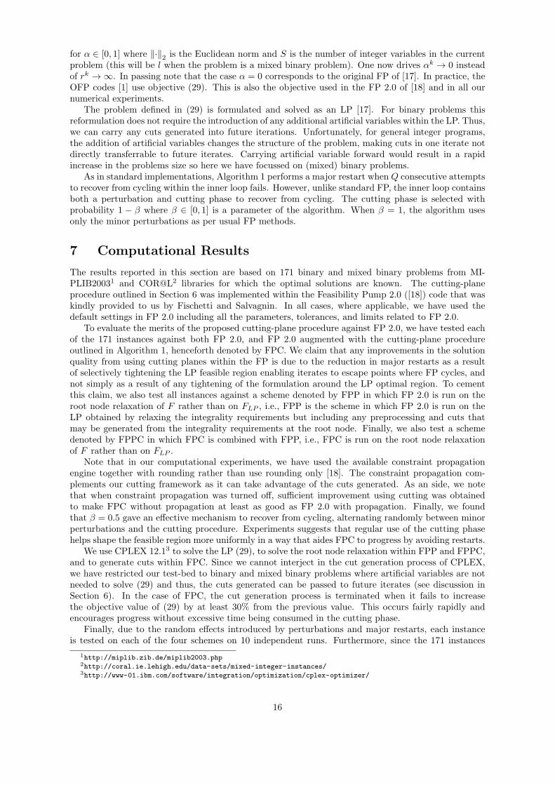
present problems that pose varied levels of difficulty for FP 2.0, we classify each of the 171 instancesinto one of three classes depending on the number of major restarts needed before an integer feasiblesolution is obtained using standard FP 2.0. Class A includes 110 problems that terminated with nomajor restarts for at least 7 out of the 10 runs, Class B 30 problems not in class A with less than 10major restarts for at least 7 out of 10 runs, and Class C the remaining 31 problems.

FP 2.0 FPP FPC FPPC

Class A 0.02 0.18 0.18 0.12Class B 2.9 13.43 0.83 1.70Class C 93.3 99.6 3.1 2.76

Table 1: Average number of major restarts for each scheme over all runs associated with instancesbelonging to each class

Table 1 reports the average number of major restarts for each scheme over all runs associated withinstances belonging to a given class. Hence, if IA, IB , and IC are the set of instances belonging to classA, B, and C respectively, S = {FP 2.0, FPP, FPC, FPPC} is the set of schemes, and Rs

ij is the number

of major restarts observed during the jth (out of 10) run of instance i using some scheme s ∈ S, thenfor each scheme s ∈ S and class l ∈ {A,B,C}, Table 1 reports

Rsl =

1

10|Il|∑i∈Il

10∑j=1

Rsij .

Additionally, the box plots given in Figure 1, gives the distribution of the average (over the 10 inde-pendent runs for each instance) number of major restarts by scheme and problem class. More precisely,for each class l ∈ {A,B,C}, and each scheme s ∈ S, Figure 1 plots the distribution of points 1

10

10∑j=1

Rsij : i ∈ Il

.

To present a clearer picture, Figure 1 includes box plots of these distributions with and without outliers.Points are considered as outliers if they are larger than q3+1.5(q3−q1) or smaller than q1−1.5(q3−q1),where q1 and q3 are the 25th and 75th percentiles, respectively. These outliers correspond to a smallfraction of the overall data (approximately 0.7% of the data if the data is approximately normallydistributed).

From Table 1 and Figure 1 it is clear that adding cuts strategically at points where FP cycles has adramatic effect on reducing the number of major restarts for problems in classes B and C. FPP, FPCand FPPC all increase the average number of major restarts for problems in class A. However, as canbe observed from Figure 1, this is mainly due to a handful of outliers. For problems in class B, FPCreduces the number of major restarts by more than a factor of three on average however, both FPPand FPPC have more restarts than FP 2.0 and FPC respectively. This is not completely surprising.Indeed, tightening the formulation through cuts at the root node is likely to make the relaxation morefractional. The binary knapsack problem is a classic example of this. Here, the LP relaxation has onlyone fractional variable whereas any strengthening of the problem with the addition of cuts is likely tointroduce greater fractionality. Similarly, for problems in class C, FPC reduces the number of majorrestarts by more than a factor of thirty over FP 2.0 on average whereas FPPC and FPP are comparableto FPC and FP 2.0 respectively. Finally, it is worth noting that although the number of major restartsis reduced significantly, the overall number of FP iterations remains comparatively unchanged withinthe various schemes. We next present the main results demonstrating the impact of the reduction inmajor restarts on solution quality and thus, the efficacy of the proposed cutting scheme.

Figures 2 and 3 provide performance profiles for the average and best solutions obtained respectivelyby the various schemes and for the various class of problems. Each plot gives the percentage of instanceswhere a solution was obtained by a given scheme within a certain percentage to the optimal solution.More precisely, if Js

i ⊆ {1, . . . , 10} is the subset of runs of scheme s for instance i that produced asolution, and Zs

ij is the objective value of the best solution found for instance i during run j ∈ Jsi , then

we define

Zsi =

1

|Jsi |

∑j∈Js

i

Zsij

17

05

1015

FP 2.0 FPP FPC FPPC

Class A

0

1

2

FP 2.0 FPP FPC FPPC

Class A (without outliers)

050

100150

FP 2.0 FPP FPC FPPC

Class B

0246

FP 2.0 FPP FPC FPPC

Class B (without outliers)

0200400600

FP 2.0 FPP FPC FPPC

Class C

0100200300

FP 2.0 FPP FPC FPPC

Class C (without outliers)

Figure 1: Distribution of the average number of major restarts by scheme and problem class

to be the average objective value of solutions found for instance i using scheme s, and

Zsi = max

j∈Jsi

Zsij

to be the best objective value among solutions found for instance i using scheme s. We set Zsi and Zs

i

to ∞ if Jsi = {∅}. Moreover, given Z∗

i , the optimal solution for instance i, the percentage gap to theaverage objective value of solutions found for instance i using scheme s is given by

avgGapsi =(Zs

i − Z∗i )

Z∗i + 1

× 100,

and similarly, the percentage gap to the best solution found for instance i using scheme s is given by

bestGapsi =(Zs

i − Z∗i )

Z∗i + 1

× 100.

Then, for each percentage p ∈ [0, 100] and scheme s, Figure 2 plots the number of instances whoseaverage objective is within p percent of the optimal solution, i.e. plots p against the number of instancesi that have avgGapsi ≤ p. Similarly, Figure 3 plots the number of instances i whose best objective iswithin p percent of the optimal solution, i.e. plots the number of instances i where bestGapsi ≤ p.Figures 2(a) and 3(a) present this information over all instances for each of the four schemes whileFigures 2(b)-2(d) and 3(b)-3(d) present this information for problems in each of the three classes A, B,and C respectively.

Although there is not much that separates FPC and FPPC, from Figures 2(a) and 3(a) it is clearthat on the whole, the cutting plane approaches outperform FP 2.0 and FPP. When examining the threeclasses in isolation, we observe that for problems in class A, it is the tightening of the feasible region(FPP) that yields most of the improvement. This is to be expected as an attempt to reduce majorrestarts (FPC, FPPC) cannot be very useful for problems that do not require many major restarts tobegin with. Here FPC does worse than FPP but better than FP 2.0 while FPPC does better thanFPP. The true impact of the proposed cutting scheme as a mechanism for recovering from cycling isevident for the harder problems within classes B and C. Indeed, the percentage of problems that could

18

0

10

20

30

40

50

60

70

80

90

10

0 0 2

0 4

0 6

0 8

0 1

00

12

0 1

40

16

0 1

80

20

0

% of problems

FP

2 (

av

er)

FP

P (

av

er)

FP

PC

(a

ve

r)F

PC

(a

ve

r)

% g

ap

to

op

tim

al s

olu

tio

n

(a) All problems

0

10

20

30

40

50

60

70

80

90

10

0

0 2

0 4

0 6

0 8

0 1

00

12

0 1

40

16

0 1

80

20

0% of problems

% g

ap

to

op

tim

al s

olu

tio

n

FP

2 (

av

er)

FP

P (

av

er)

FP

PC

(a

ve

r)F

PC

(a

ve

r)

(b) Class A

10

20

30

40

50

60

70

80

90

0 2

0 4

0 6

0 8

0 1

00

12

0 1

40

16

0 1

80

20

0

% of problems

% g

ap

to

op

tim

al s

olu

tio

n

FP

2 (

av

er)

FP

P (

av

er)

FP

PC

(a

ve

r)F

PC

(a

ve

r)

(c) Class B

0

10

20

30

40

50

60

70

80

0 2

0 4

0 6

0 8

0 1

00

12

0 1

40

16

0 1

80

20

0

% of problems

% g

ap

to

op

tim

al s

olu

tio

n

FP

2 (

av

er)

FP

P (

av

er)

FP

PC

(a

ve

r)F

PC

(a

ve

r)

(d) Class C

Figure 2: Percentage of instances where the average value of solutions obtained over the 10 independentruns by a given scheme is within a certain percentage to the optimal solution.

19

10

20

30

40

50

60

70

80

90

10

0 0 2

0 4

0 6

0 8

0 1

00

12

0 1

40

16

0 1

80

20

0

% of problems

% g

ap

to

op

tim

al s

olu

tio

n

FP

2 (

be

st)

FP

P (

be

st)

FP

PC

(b

est

)F

PC

(b

est

)

(a) All problems

10

20

30

40

50

60

70

80

90

10

0 0 2

0 4

0 6

0 8

0 1

00

12

0 1

40

16

0 1

80

20

0% of problems

% g

ap

to

op

tim

al s

olu

tio

n

FP

2 (

be

st)

FP

P (

be

st)

FP

PC

(b

est

)F

PC

(b

est

)

(b) Class A

10

20

30

40

50

60

70

80

90

0 2

0 4

0 6

0 8

0 1

00

12

0 1

40

16

0 1

80

20

0

% of problems

% g

ap

to

op

tim

al s

olu

tio

n

FP

2 (

be

st)

FP

P (

be

st)

FP

PC

(b

est

)F

PC

(b

est

)

(c) Class B

0

10

20

30

40

50

60

70

80

90

10

0 0 2

0 4

0 6

0 8

0 1

00

12

0 1

40

16

0 1

80

20

0

% of problems

% g

ap

to

op

tim

al s

olu

tio

n

FP

2 (

be

st)

FP

P (

be

st)

FP

PC

(b

est

)F

PC

(b

est

)

(d) Class C

Figure 3: Percentage of instances where the value of the best solution obtained over the 10 independentruns by a given scheme is within a certain percentage to the optimal solution.

20

be solved to within 10% of optimality is almost twice that in FPC and FPPC as compared to FP 2.0for class C, and almost 50% more for problems in class B.

Admittedly, by examining the relative performance of FPP versus FP 2.0, we can conclude thatsome of the aforementioned gains can be attributed to simply tightening the formulation at the rootnode. However, there are significant gains to be had over FPP by using cutting planes strategically toavoid cycling. When comparing the average objective values obtained over the 10 independent runs,FPC is better on 21 occasions, and worse on only 3 occasions for the 30 instances belonging to ClassB., i.e., |{i ∈ IB : ZFPC

i < ZFP2.0i }| = 21 and |{i ∈ IB : ZFPC

i > ZFP2.0i }| = 3. For the same measure,

FPC is better on 24 occasions and worse on only 6 occasions for the 31 instances in Class C. Moreover,when comparing the best objective value found over the 10 independent runs for instances in Class C,FPC was better than FP 2.0 on 26 occasions and worse on only 4 occasions, i.e., |{i ∈ IC : ZFPC

i <

ZFP2.0i }| = 26 and |{i ∈ IC : ZFPC

i > ZFP2.0i }| = 4. Even if we compare the best solution found

by FP 2.0 over the 10 independent runs with the average solution found by FPC, the comparison stilllooks favorable for FPC yielding 18 wins and 12 losses, i.e., |{i ∈ IC : ZFPC

i < ZFP2.0i }| = 18 and

|{i ∈ IC : ZFPCi > ZFP2.0

i }| = 12. Finally, it is worth noting that FPC failed to find a feasible solutionin all 10 runs for only one instance (for which FP 2.0 also failed), while FP 2.0 failed to find a feasiblesolution in all 10 runs for 5 problems. The reader is referred to Appendix B and the tables therein thatprovide detailed statistics comparing the results of FP 2.0 with FPC for individual instances.

FP 2.0 FPP FPC FPPC

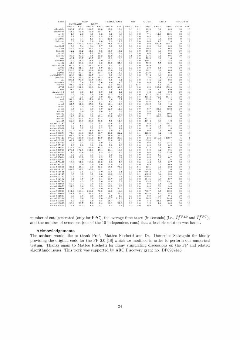
Class A 24.23 43.91 32.11 49.72Class B 13.07 21.60 81.58 81.73Class C 18.52 23.65 63.46 69.38

Table 2: Average time (in seconds) taken by each scheme over all runs associated with instancesbelonging to given class

Of course, the gains in terms of solution quality obtained from using cuts to tighten the formulationand/or recover from cycling comes at a cost in particular, the additional computational effort requiredin cut generation. Table 2 reports the average time (in seconds) for each scheme over all runs associatedwith instances belonging to a given class. Hence, if T s

ij is the time taken for the jth (out of 10) runof instance i using some scheme s ∈ S, then for each scheme s ∈ S and class l ∈ {A,B,C}, Table 2reports

T sl =

1

10|Il|∑i∈Il

10∑j=1

T sij .

The box plots given in Figure 4, gives the distribution of the average (over the 10 independent runsfor each instance) time taken by each scheme for problems in each class. More precisely, for each classl ∈ {A,B,C}, and each scheme s ∈ S, Figure 1 plots the distribution of points 1

10

10∑j=1

T sij : i ∈ Il

.

As before, 4 includes box plots with and without outliers.From Table 2 and Figure 4 it is clear that incorporating cut generation within FP places a heavy

burden on the computational effort required. However, almost all of the reported increase in time is dueto the cut generation process itself. Hence, we are optimistic that through further tuning and a propersoftware solution/integration of the cutting procedure with FP (as we are using CPLEX as a “blackbox” only), any additional computational burden is likely to pay dividends in practical situations wheretime may also be of the essence.

8 Further Directions

The connection of FP methods with proximal point algorithms, and the theoretical results we havepresented here, motivate several new directions of exploration for future research. One of our keyinsights is that the FP pumping cycle appears to be seeking local minima of a weighted combination ofthe original objective function and a measure of integrality. The method cycles at LP feasible points

21

0500

10001500

FP 2.0 FPP FPC FPPC

Class A

0

20

40

60

FP 2.0 FPP FPC FPPC

Class A (without outliers)

0500

10001500

FP 2.0 FPP FPC FPPC

Class B

0

20

40

FP 2.0 FPP FPC FPPC

Class B (without outliers)

0

500

1000

FP 2.0 FPP FPC FPPC

Class C

0

50

100

FP 2.0 FPP FPC FPPC

Class C (without outliers)

Figure 4: Distribution of the average time taken (in seconds) by each scheme for problems in each class

which are either local minima, or have multiple alternate roundings. Alternate roundings could breakthe cycle; if this is not possible then the point must be a local minimum. This insight motivates adifferent approach to the FP minor perturbation step, which chooses at random a number of variablesto have their rounding changed, and changes those variables with fractional values closest to 0.5. Sincevariables at 0.5 are precisely those causing alternative roundings, it thus seems that minor perturbationhas two functions: (a) to carry out a randomized search of the set of alternative roundings when theseare not unique, to check whether or not the algorithm is likely to be at a local minimum, and (b)to escape the local minimum. If the number of variables to have their rounding changed exceeds thenumber at or near 0.5, then it is (b) that is occurring, otherwise it is (a). Since the minor perturbationstep does not look at the number of variables at or near 0.5, there is an opportunity to re-design thisstep: do (a) until there is convincing evidence the current point is like to be a local minimum, andthen (b) escape it. It could be that current minor perturbation is doing (a) quite well, and our cuttingapproach is doing (b) well, but in both standard FP methods and our cutting plane modification, stepsof (a) and (b) occur in a mixed sequence.

Another direction of further research is to explore the role of the weighting parameter, that weightsintegrality versus the original objectives. Current FP methods simply increase this parameter to in-creasingly emphasize integrality. However the theoretical results show that optimal solutions requirethe parameter to be sufficiently small. It seems likely that further experimentation with how this pa-rameter is adjusted could yield more effective algorithms, and in particular that phases in which theparameter is also decreased may be beneficial to producing higher quality solutions.

A Proof of Proposition 7

Proof. In view of Lemma 5 part 3 we need only show that if x = y0 is the unique solution of (13) fory = y0 then it is a strict local minimum of φr. Note that we already know that y0 is integral. ConsiderK := φr (y0) + 2 and denote

F IK (y0) :=

{xI ∈ I | inf

xI∈Rn−m{f (xI , xR) + rρ ((xI , xR)− y0)} ≤ K

}

22

which is bounded due to the fact that FK (y0) as defined in (15) is bounded. Now y 7→ φr (y) is uppersemi-continuous when y 7→ ρ (x− y) is continuous. Thus y close to y0 we have φr (y)+1 < φr (y0)+2 =K. Consequently for y sufficiently close to y0 we have F I

K−1 (y) ⊆ F IK (y0). Using the discreteness of

the integral part of the solutions in F IK(y0) and that y0 is the unique minimum we have some ε > 0

such that

f (x) + rρ (x− y0) ≥ infxR∈Rn−m

{f (xI , xR) + rρ ((xI , xR)− y0)}

≥ f (y0) + 2ε = φr (y0) + 2ε for all xI = (y0)I with xI ∈ F IK (y0) .

By lower semi-continuity of ρ and compactness of FK , for y sufficiently close to y0 and all x withx ∈ FK (y0) we have

rρ (x− y) ≥ rρ (x− y0)− ε. (30)

Consequently for all y sufficiently close to y0

f (x) + rρ (x− y) ≥ φr (y0) + ε for all xI = (y0)I with xI ∈ F IK (y0) .

Thus minx{f (x) + rρ (x− y) | (y0)I = xI with xI ∈ F I

K (y0)}≥ φr (y0)+ε for all y close to y0. Using

F IK−1 (y) ⊆ F I

K (y0) for y sufficiently close to y0 we have

φr (y) =

min{ minx:xI =(y0)I

{f (x) + rρ (x− y) | xI ∈ F I

K−1 (y)}

, minx:xI=(y0)I

{f (x) + rρ (x− y) | xI ∈ F I

K−1 (y)}}

≥ min{ minx:xI =(y0)I

{f (x) + rρ (x− y) | xI ∈ F I

K−1 (y)}

,minxR{f ((y0)I , xR) + rρ (xR − yR) + rρ ((y0)I − yI)}}

≥ min {φr (y0) + ε,Gr (yR) + rρ ((y0)I − yI)} . (31)

Now note that

Gr ((y0)R) ≥ φr (y0) = f (y0)

≥ minzR∈Rn−m

{f ((y0)I , zR) + rρ (((y0)I , zR)− y0)} = Gr ((y0)R)

so Gr ((y0)R) = φr (y0). Also (y0)R is a local minimum of Gr because Gr (yR) ≥ φr ((y0)I , yR) for ally and y0 is a local minimum of φr i.e. for yR close to (y0)R

Gr (yR) ≥ φr ((y0)I , yR) ≥ φr (y0) = Gr ((y0)R) .

Thus for y sufficiently close to y0 we have φy(y) ≥ φr(y0).When we have an IP then Gr (yR) = φr (y0) and so we have

φr (y) ≥ min {φr (y0) + ε, φr (y0) + rρ (y0 − y)} .

Thus we have a strict local minimum at y0. Further more in the more general case of a MIP when(y0)R is a strict local minimum of Gr then the inequality in (31) again implies y0 must also be a strictlocal minimum of φr.

B Detail results for FP 2.0 and FPC

In Tables 3, 4, and 5 we report detailed statistics related to the runs associated with FP 2.0 and FPCfor each of the 171 instances. The first column gives the problem’s name, and for each of the twoschemes FP 2.0 and FPC, the remaining columns give the average gap to the optimal solution over the10 independent runs (i.e., avgGapFP2.0

i and avgGapFPCi ), the gap to the optimal solution from the

best solution obtained over the 10 independent runs (i.e., bestGapFP2.0i and bestGapFPC

i ), the averagenumber of FP iterations, the average number of major restarts (i.e., RFP2.0

i and RFPCi ), the average

23

name GAP ITERATIONS MR CUTS TIME SUCCESS

AVERAGE BESTFP2.0 FPC FP2.0 FPC FP2.0 FPC FP2.0 FPC FPC FP2.0 FPC FP2.0 FPC

aflow30a 133.1 63.9 104.7 18.6 17.9 15.4 0.0 0.1 12.9 0.1 0.5 10 10aflow40b 41.5 53.0 16.9 15.3 8.3 16.2 0.0 0.1 16.1 0.1 1.5 9 10

air04 1.4 2.3 0.1 0.6 8.2 8.6 0.0 0.0 7.1 11.9 13.5 10 10air05 2.8 3.7 1.5 1.5 6.8 9.3 0.0 0.0 0.5 3.0 4.4 10 10

cap6000 2.3 0.4 1.3 0.4 29.6 16.3 0.0 0.0 1.5 0.8 3.0 9 10disktom 0.0 0.0 0.0 0.0 1.9 1.9 0.0 0.0 0.0 1.8 1.8 9 9

ds 961.0 747.7 553.3 442.4 78.8 80.5 0.0 0.0 0.0 599.8 552.1 10 10fast0507 5.0 5.4 3.4 1.7 3.9 3.6 0.0 0.0 0.0 8.4 8.8 10 10

fiber 244.3 45.9 133.1 3.8 17.3 7.3 0.0 0.0 19.4 0.1 0.5 10 10fixnet6 12.2 15.2 11.3 7.3 15.0 14.7 0.0 0.0 18.8 0.0 0.8 10 10harp2 9.3 11.0 7.1 10.7 11.9 9.4 0.0 0.0 6.0 0.1 0.5 10 10

misc07 36.6 37.3 6.6 11.2 21.9 14.6 0.1 0.0 11.6 0.1 0.6 10 10mkc 49.7 23.7 49.7 13.1 11.2 10.0 0.0 0.0 75.9 0.2 1.6 1 10

mod011 16.5 11.3 11.8 2.0 11.7 12.5 0.0 0.0 419.1 0.3 3.2 10 10net12 41.0 28.6 19.1 0.0 31.9 27.0 0.4 0.0 59.9 7.5 8.3 10 10

nsrand-ipx 60.9 34.3 47.2 24.4 9.4 7.6 0.0 0.0 36.9 0.5 2.1 10 10nw04 31.2 21.4 5.9 5.9 13.4 9.3 0.0 0.0 2.0 3.5 7.0 10 10p2756 123.3 30.6 59.6 20.8 15.0 5.1 0.0 0.0 18.1 0.1 0.6 10 10pp08a 63.9 27.7 41.4 10.7 10.8 11.3 0.0 0.0 114.9 0.0 0.7 10 10

pp08aCUTS 38.6 21.4 22.7 4.4 9.9 10.8 0.0 0.0 61.4 0.0 0.6 10 10protfold 52.8 57.2 43.8 31.3 18.9 34.9 0.0 0.1 3.0 10.8 23.5 10 10

qiu 496.7 478.0 68.7 167.1 8.0 8.1 0.0 0.0 1.6 0.2 0.8 10 10seymour 3.6 3.4 2.8 2.6 4.6 4.8 0.0 0.0 0.8 2.4 2.6 10 10

sp97ar 21.3 17.8 17.4 15.4 9.3 67.0 0.0 12.7 4.1 3.1 25.1 10 9t1717 149.3 151.9 99.3 34.6 36.5 38.8 0.0 0.0 0.0 147.2 159.4 10 10

bc1 28.0 20.4 2.4 2.4 7.8 8.1 0.0 0.0 2.9 1.2 6.0 10 9binkar10-1 6.5 6.8 1.0 1.0 6.2 1.7 0.0 0.0 1.2 0.1 0.2 10 10

dano3-3 0.0 0.0 0.0 0.0 12.3 12.8 0.0 0.0 47.2 36.7 103.2 10 10dano3-5 0.0 0.1 0.0 0.0 21.4 34.1 0.0 0.7 315.4 72.1 341.1 10 10

leo1 34.0 17.8 17.6 11.9 8.6 5.7 0.0 0.0 12.0 0.7 1.9 10 10leo2 28.9 15.3 15.8 2.7 8.3 6.4 0.0 0.0 15.6 1.4 3.7 10 10

neos1 37.5 11.0 35.0 5.0 12.4 11.6 0.0 0.0 100.2 0.1 1.3 10 10neos5 4.7 5.5 0.0 0.0 5.6 6.3 0.0 0.0 1.3 0.0 0.6 10 10neos9 0.5 0.4 0.0 0.0 12.0 11.3 0.0 0.0 9.7 24.3 62.2 10 10

neos11 0.0 0.0 0.0 0.0 8.1 6.2 0.0 0.0 5.0 1.1 1.7 10 10neos12 15.7 35.7 7.1 7.1 4.9 6.9 0.0 0.0 0.0 6.2 10.6 10 10neos13 14.5 30.3 0.3 19.4 28.0 26.8 0.0 0.0 1.1 32.8 63.6 10 10neos14 46.0 45.1 35.5 27.7 7.3 9.3 0.0 0.0 331.7 0.0 1.1 10 10neos15 52.0 46.1 39.0 30.5 7.5 11.9 0.0 0.0 341.4 0.0 1.2 10 10

neos-476283 0.1 0.2 0.1 0.1 10.6 12.4 0.0 0.0 8.4 110.5 194.1 10 10neos-480878 2.4 1.3 0.3 0.3 13.0 9.8 0.0 0.0 15.2 0.5 2.1 10 10neos-495307 5.7 5.7 5.7 5.7 7.1 7.2 0.0 0.0 1.4 0.3 1.8 10 10neos-503737 49.2 45.7 18.9 30.2 3.9 3.2 0.0 0.0 0.0 0.6 0.6 10 10neos-504674 77.4 64.6 24.5 31.7 29.6 32.2 0.0 0.1 213.8 0.2 1.3 10 10neos-504815 68.4 40.8 42.0 10.7 28.0 27.9 0.0 0.0 113.5 0.1 1.1 10 10neos-506428 176.0 135.0 160.0 40.0 25.3 33.8 0.0 0.0 2.8 1316.8 1482.7 5 4neos-512201 62.7 67.2 20.8 14.1 28.6 27.8 0.0 0.0 169.6 0.2 1.1 10 10neos-520729 0.3 0.4 0.2 0.0 4.4 4.9 0.0 0.0 0.0 3.7 27.4 10 10neos-525149 2.6 2.6 0.0 0.0 1.0 1.0 0.0 0.0 0.0 0.1 0.2 10 10neos-538867 177.6 164.2 65.0 81.3 15.5 13.3 0.0 0.0 11.3 0.1 0.4 10 10neos-538916 276.1 172.5 151.1 47.4 20.4 16.8 0.0 0.0 6.0 0.2 0.5 10 10neos-544324 11.3 10.6 6.3 6.3 15.2 18.9 0.0 0.0 0.0 5.9 22.0 10 10neos-547911 8.6 7.1 7.1 7.1 5.2 5.2 0.0 0.0 0.0 1.3 1.7 10 10neos-555694 22.7 23.5 6.2 6.2 5.2 9.2 0.0 0.0 0.0 0.2 0.7 10 10neos-565815 0.0 0.0 0.0 0.0 3.8 4.4 0.0 0.0 2.2 1.2 1.6 10 10neos-570431 13.0 17.0 10.0 10.0 6.8 7.3 0.0 0.0 4.4 0.3 0.7 10 10neos-584146 0.0 0.0 0.0 0.0 15.0 14.1 0.0 0.0 6.8 0.2 0.9 10 10neos-584851 26.7 45.4 0.0 33.3 17.8 75.9 0.0 5.4 12.1 0.3 2.2 10 9neos-611135 187.8 122.7 50.8 50.1 14.1 10.5 0.0 0.0 15.0 3.3 7.6 10 10neos-611838 0.7 0.5 0.7 0.0 10.5 6.8 0.0 0.0 618.2 0.4 2.0 10 10neos-612125 0.5 0.5 0.5 0.0 10.8 10.8 0.0 0.1 582.0 0.4 2.8 10 10neos-612143 0.7 0.5 0.7 0.0 10.7 9.1 0.0 0.0 629.6 0.4 2.8 10 10neos-612162 0.7 0.7 0.7 0.1 10.7 8.6 0.0 0.0 644.5 0.4 2.7 10 10neos-631784 8.6 4.3 3.9 2.0 16.8 15.8 0.0 0.0 113.5 3.5 13.1 10 10neos-691058 56.4 0.4 0.0 0.3 14.1 10.0 0.0 0.0 0.0 2.8 4.0 10 10neos-691073 21.3 0.6 0.3 0.3 10.3 8.3 0.0 0.0 0.0 3.0 3.4 10 10neos-738098 0.0 0.0 0.0 0.0 23.5 20.3 0.0 0.0 2.0 14.7 26.9 10 10neos-787933 311.9 158.4 283.9 71.0 19.0 19.0 0.0 0.0 789.7 3.7 10.0 10 10neos-791021 48.1 26.2 37.5 6.3 29.7 27.4 0.0 0.0 453.5 1.0 8.5 10 10neos-801834 6.6 6.6 6.0 6.6 1.0 1.0 0.0 0.0 0.0 0.4 0.4 10 10neos-808214 0.0 0.0 0.0 0.0 110.7 111.8 1.2 0.0 10.5 13.0 14.6 10 10neos-810286 8.3 5.2 3.9 0.5 18.7 15.0 0.0 0.0 5.4 21.1 19.2 10 10neos-810326 20.0 29.7 7.0 2.4 16.1 21.9 0.0 0.0 1.9 4.4 8.0 10 10neos-820879 14.1 13.5 8.0 7.1 9.5 7.1 0.0 0.0 0.9 0.9 1.0 10 10

number of cuts generated (only for FPC), the average time taken (in seconds) (i.e., TFP2.0i and TFPC

i ),and the number of occasions (out of the 10 independent runs) that a feasible solution was found.

AcknowledgementsThe authors would like to thank Prof. Matteo Fischetti and Dr. Domenico Salvagnin for kindlyproviding the original code for the FP 2.0 [18] which we modified in order to perform our numericaltesting. Thanks again to Matteo Fischetti for many stimulating discussions on the FP and relatedalgorithmic issues. This work was supported by ARC Discovery grant no. DP0987445.

24

name GAP ITERATIONS MR CUTS TIME SUCCESS

AVERAGE BESTFP2.0 FPC FP2.0 FPC FP2.0 FPC FP2.0 FPC FPC FP2.0 FPC FP2.0 FPC

neos-824695 2.2 0.6 0.0 0.0 8.9 5.2 0.0 0.0 0.5 3.3 3.9 10 10neos-825075 22.3 12.1 0.0 0.0 6.8 5.5 0.0 0.0 0.8 0.1 0.1 10 10neos-826250 0.7 0.0 0.0 0.0 4.1 3.5 0.0 0.0 0.6 1.3 1.6 10 10neos-826812 0.5 0.2 0.0 0.0 4.7 2.9 0.0 0.0 0.5 2.4 2.6 10 10neos-827015 63.7 117.0 33.9 37.4 3.8 6.3 0.0 0.0 0.0 48.4 73.0 10 10neos-827175 0.0 0.0 0.0 0.0 1.0 1.0 0.0 0.0 0.0 2.5 2.3 10 10neos-829552 68.2 68.2 68.2 68.2 1.0 1.0 0.0 0.0 0.0 11.7 11.9 10 10neos-841664 18.4 3.9 3.1 0.0 18.9 9.8 0.3 0.0 235.0 4.9 6.8 10 10neos-847302 12.0 0.0 0.0 0.0 12.6 10.2 0.0 0.0 2.2 1.2 1.3 10 10neos-860300 36.3 36.1 36.2 35.7 3.0 3.0 0.0 0.0 0.0 0.6 0.9 10 10neos-885524 7.3 5.1 0.0 0.0 38.7 0.9 3.2 0 0neos-892255 13.3 12.0 13.3 0.0 6.0 5.6 0.0 0.0 0.0 0.3 0.5 10 10neos-906865 0.0 7.6 0.0 0.0 7.9 8.4 0.0 0.0 2.9 0.1 0.5 10 10neos-932816 0.0 0.0 0.0 0.0 3.1 2.5 0.0 0.0 0.0 4.1 3.9 9 10neos-933364 6.9 6.9 5.6 5.4 6.5 6.5 0.0 0.0 14.2 0.1 0.9 10 10neos-933562 20.5 26.8 0.0 0.0 16.5 15.5 0.0 0.0 0.0 1.9 2.0 10 10neos-933815 7.3 6.6 5.5 4.1 7.1 6.2 0.0 0.0 0.0 0.1 0.3 10 10neos-933966 226.1 50.8 13.0 10.1 9.8 5.0 0.0 0.0 1.0 7.2 7.1 10 10neos-934184 6.5 7.2 4.7 5.0 7.0 6.6 0.0 0.0 14.2 0.1 0.8 10 10neos-934278 72.0 145.0 25.1 26.5 4.2 6.3 0.0 0.0 0.0 7.8 9.5 10 10neos-934441 54.2 58.4 24.1 31.2 7.6 4.4 0.0 0.0 0.0 10.4 9.5 10 10neos-935234 42.6 52.7 20.0 22.9 4.9 5.4 0.0 0.0 0.0 10.0 10.3 10 10neos-935348 37.2 55.1 21.1 17.3 4.5 4.0 0.0 0.0 1.5 9.3 8.9 10 10neos-935674 2672.3 2427.7 1600.0 784.6 8.1 6.5 0.0 0.0 1.0 1.0 1.1 10 10neos-935769 5.5 4.4 2.4 0.8 7.4 6.8 0.0 0.0 6.9 17.9 18.8 10 10neos-941698 113.3 133.3 0.0 0.0 21.5 17.2 0.0 0.0 2.0 0.7 0.8 10 10neos-941782 18.9 23.7 5.3 0.0 18.9 19.6 0.0 0.0 8.8 1.0 1.5 10 10neos-942323 26.7 25.6 16.7 16.7 19.9 25.0 0.0 0.0 6.0 0.3 0.6 10 10neos-948268 0.0 0.0 0.0 0.0 3.5 3.6 0.0 0.0 0.0 10.6 10.7 10 10neos-955215 2.2 1.7 0.4 0.4 4.3 4.6 0.0 0.0 2.4 0.0 0.3 10 10neos-957323 0.2 0.3 0.0 0.0 5.3 4.6 0.0 0.0 0.5 5.7 19.1 10 10

neos-1067731 0.6 5.4 0.4 0.4 5.1 5.8 0.0 0.0 0.3 2.4 4.4 10 10neos-1109824 55.2 43.3 37.7 8.2 24.7 18.4 0.7 0.2 45.0 0.7 1.8 10 10neos-1171448 1.1 0.6 0.3 0.0 14.8 13.2 0.0 0.0 20.5 2.0 18.2 10 10neos-1200887 12.3 8.8 5.3 2.7 11.4 13.6 0.0 0.0 12.8 0.1 1.0 10 10neos-1211578 4.5 2.7 2.6 1.3 13.6 10.9 0.0 0.0 12.2 0.0 0.7 10 10

Table 3: Detailed statistics for FP2.0 and FPC for problems in class A

name GAP ITERATIONS MR CUTS TIME SUCCESS

AVERAGE BESTFP2.0 FPC FP2.0 FPC FP2.0 FPC FP2.0 FPC FPC FP2.0 FPC FP2.0 FPC

10teams 10.9 9.7 4.5 3.2 109.0 89.3 2.0 0.0 6.7 7.3 6.6 10 10dano3mip 12.2 7.9 6.9 6.1 68.5 85.9 0.4 0.1 5994.9 330.2 1536.6 10 4

markshare1 21280.0 13560.0 10950.0 6100.0 68.4 67.9 3.4 0.7 68.1 0.1 2.8 10 10markshare2 29555.0 19915.0 13350.0 12800.0 70.0 69.7 3.0 0.3 64.4 0.2 3.1 10 10

opt1217 3.5 0.0 0.0 0.0 38.3 33.7 0.6 0.1 7.1 0.1 1.3 10 10pk1 526.7 105.5 250.0 58.3 57.6 278.8 1.4 0.6 294.3 0.2 13.1 10 9

swath 163.8 130.3 65.1 35.5 162.5 370.5 5.0 0.1 606.2 10.1 231.5 10 6tr12-30 27.5 37.2 23.5 22.6 27.0 21.4 0.3 0.0 835.6 0.1 3.3 10 10

vpm2 25.4 18.1 11.9 3.4 17.0 11.6 0.4 0.0 26.2 0.0 0.5 10 1022433 0.3 0.1 0.0 0.0 65.0 67.8 6.1 0.2 18.7 0.3 1.4 10 1023588 2.4 1.9 1.1 1.0 91.8 71.7 4.3 0.1 7.7 0.3 0.8 10 10

bienst1 13.7 12.8 0.0 0.0 53.5 102.8 2.7 0.5 537.2 0.5 34.6 10 10bienst2 14.7 7.4 9.1 2.1 54.7 79.4 2.5 0.6 578.7 0.6 24.9 10 10

mcf2 19.0 22.5 1.1 9.5 96.2 455.4 20.4 0.3 2403.2 2.7 449.7 10 7neos-522351 36.8 2.3 19.2 0.0 50.4 27.1 1.8 1.7 263.8 0.4 3.0 10 10neos-582605 0.0 0.0 0.0 0.0 67.5 45.5 2.6 0.4 80.5 0.8 8.8 10 10neos-583731 0.0 0.0 0.0 0.0 37.9 43.5 0.1 0.0 190.6 0.2 1.4 10 10neos-631164 11.6 11.9 7.0 8.9 75.8 70.0 1.2 0.2 64.5 0.4 1.0 10 10neos-631517 10.3 10.1 7.5 8.7 75.4 72.7 0.9 0.4 53.5 0.3 0.9 10 10neos-777800 0.0 0.0 0.0 0.0 21.5 32.6 0.7 0.4 2.6 9.3 16.3 10 10neos-831188 9.0 11.2 1.3 1.2 137.8 176.5 4.4 0.0 30.7 11.9 21.7 10 10neos-839838 33.9 22.4 12.9 9.3 56.9 234.4 6.7 15.0 124.9 3.6 51.8 10 8neos-839859 235.9 39.7 61.8 13.0 42.2 19.3 1.5 0.2 30.9 0.5 2.0 10 10neos-886822 44.9 38.7 24.2 22.4 114.0 112.2 3.3 0.5 27.2 2.0 5.0 10 10neos-911880 206.4 50.9 149.6 11.0 51.0 36.7 1.0 0.6 101.1 0.1 2.0 10 10neos-911970 225.9 43.9 112.9 11.2 50.2 39.3 0.9 0.8 126.0 0.2 1.6 10 10neos-912015 49.3 51.3 26.7 20.0 164.9 188.5 2.6 0.0 7.7 8.7 11.2 10 10

neos-1053234 70.3 32.0 42.9 17.4 39.1 34.6 4.5 0.8 112.7 0.4 6.7 10 10neos-1120495 56.1 50.7 21.2 18.5 17.3 14.7 0.1 0.0 35.1 0.4 1.1 10 10neos-1121679 2634.7 1582.4 1417.6 658.8 68.3 69.7 2.2 0.5 74.9 0.1 2.9 10 10

Table 4: Detailed statistics for FP2.0 and FPC for problems in class B

25

name GAP ITERATIONS MR CUTS TIME SUCCESS

AVERAGE BESTFP2.0 FPC FP2.0 FPC FP2.0 FPC FP2.0 FPC FPC FP2.0 FPC FP2.0 FPC

a1c1s1 60.1 34.9 38.6 21.8 51.3 18.6 13.4 0.0 744.0 0.5 3.7 10 10danoint 17.5 17.9 5.0 10.2 112.3 353.5 33.8 0.3 2039.5 2.6 185.0 10 8glass4 294.6 141.9 138.9 83.3 218.3 119.1 101.9 4.1 1455.1 0.3 9.8 10 10

liu 202.8 142.6 169.4 92.9 152.2 120.1 12.9 2.1 3857.0 1.9 53.0 10 10mas74 72.3 17.7 43.1 9.1 106.2 590.7 13.9 0.4 528.6 0.1 44.3 7 5mas76 18.8 4.3 6.3 2.3 106.2 481.9 16.7 0.3 365.0 0.2 25.9 7 5

modglob 6.6×106 6.4×106 6.5×106 6.4×106 66.1 28.1 27.2 1.5 81.5 0.1 1.7 10 10set1ch 67.2 19.9 47.7 9.0 35.6 13.0 6.5 0.0 136.9 0.1 0.4 10 10

aligninq 1.3 1.4 0.9 1.3 249.4 185.6 39.3 0.0 38.6 9.1 12.6 9 9neos2 202.9 197.2 843.7 763.1 124.5 1.1 1304.7 9.5 438.0 0 3neos4 7.4 5.1 614.6 119.7 285.9 0.2 31.6 40.7 79.5 0 10

neos17 57.0 49.1 44.8 20.0 689.5 144.8 659.1 32.5 131.6 1.6 18.8 7 10neos-430149 581.7 512.6 477.0 161.8 1208.6 172.1 266.4 0.7 280.3 5.3 27.7 2 10neos-598183 159.0 25.3 103.4 0.6 318.2 133.6 49.2 0.8 380.9 3.0 10.8 7 10neos-603073 139.2 1.0 31.3 0.4 180.5 21.1 64.3 0.1 140.1 1.5 1.8 10 10neos-631694 0.0 0.0 715.8 98.9 54.7 0.1 246.6 11.0 7.4 0 10neos-803219 9.8 13.0 7.8 4.4 1110.4 368.4 79.3 12.7 221.9 3.1 38.8 2 10neos-803220 10.9 17.4 4.6 4.4 263.9 109.7 32.7 1.2 114.9 0.6 9.9 10 10neos-806323 51.1 37.9 44.5 8.7 958.6 245.7 168.1 3.8 223.9 5.3 15.5 2 10neos-807639 7.2 9.1 2.7 6.7 180.5 86.3 97.8 12.4 16.5 0.9 4.1 10 9neos-807705 18.1 21.0 8.8 15.7 129.9 56.0 34.3 0.8 72.0 0.7 4.5 10 10neos-848589 109303.8 7316.6 67846.4 526.6 68.9 51.9 10.9 2.5 1013.2 117.3 846.5 10 10neos-863472 14.2 8.4 10.2 0.7 82.9 52.7 12.9 0.1 150.5 0.3 2.3 10 10neos-880324 0.4 0.0 1053.4 240.9 380.6 6.4 320.3 1.6 7.2 0 9neos-912023 42.9 30.0 14.3 0.0 244.5 189.3 10.6 0.0 8.2 8.7 8.0 10 10neos-913984 0.0 0.0 0.0 0.0 1051.6 18.2 10.6 0.2 34.5 322.2 14.3 3 10neos-916792 26.4 16.4 10.5 7.0 227.7 121.1 24.9 0.3 40.7 22.8 68.7 9 10

neos-1053591 5.0 3.1 2.0 0.1 221.9 78.7 126.4 1.1 148.0 0.3 7.4 10 10neos-1112782 3891.8 560.9 3757.8 52.4 160.4 39.3 80.4 1.9 165.1 1.7 7.5 10 10neos-1112787 3512.3 242.8 3366.4 37.7 85.7 45.1 34.8 4.1 158.7 0.8 6.7 10 10neos-1173026 43.9 23.7 24.7 14.3 54.0 45.9 18.5 4.5 70.9 0.2 5.2 10 10

Table 5: Detailed statistics for FP2.0 and FPC for problems in class C

References

[1] T. Achterberg and T. Berthold, “Improving the Feasibility Pump”, Discrete Optimization,4(2007):77–86.

[2] E. Balas, S. Ceria, M. Dawande, F. Margot, and G. Pataki, “OCTANE: A new heuristic for pure0-1 programs”, Operations Research, 49(2001):207–225.

[3] E. Balas and C.H. Martin, “Pivot and complement-a heuristic for 0-1 programming”, ManagementScience, 26(1980):86–96.

[4] E. Balas, S. Schmieta, and C. Wallace, “Pivot and shift–a mixed integer programming heuristic”,Discrete Optimization, 1(2004):3–12.

[5] L. Bertacco, M. Fischetti and A. Lodi , “A Feasibility Pump heuristic for mixed-integerproblems”, Discrete Optimization, 4(2007):63–76.

[6] T. Berthold, Primal heuristics for mixed integer programs, Master’s thesis, Technische UniversitatBerlin, 2006.

[7] D.P. Bertsekas, Nonlinear Programming, 2nd edn. Athena Scientific, Boston, 1999.

[8] P. Bonami, G. Cornuejols, A. Lodi and F. Margot, “Feasibility Pump for mixed integer nonlinearprograms”, Mathematical Programming, 119(2009):331–352.

[9] R. S. Burachik and A.N. Iusem, Set-Valued Mappings and Enlargements of Monotone Operators,Springer Optimization and Its Applications, Vol 8, 2008.

[10] C. D′Ambrosio, A. Frangioni, L. Liberti, and A. Lodi, “Experiments with a feasibility pumpapproach for nonconvex MINLPs”, in P. Festa, editor, Symposium on Experimental Algorithms,LNCS Vol. 6049, Heidelberg, Springer, (2010): 350–360.

[11] C. D′Ambrosio, A. Frangioni, L. Liberti, and A. Lodi, “A storm of feasibility pumps for nonconvexMINLP”, 2010.

[12] A. Daniilidis and C. Lemarechal, “On a primal-proximal heuristic in discrete optimization”, Math-ematical Programming, 104(2005):105–128.

[13] E. Danna, E. Rothberg, and C.L. Pape, “Exploring relaxation induced neighborhoods to improveMIP solutions”, Mathematical Programming, 102(2005):71–90.

26

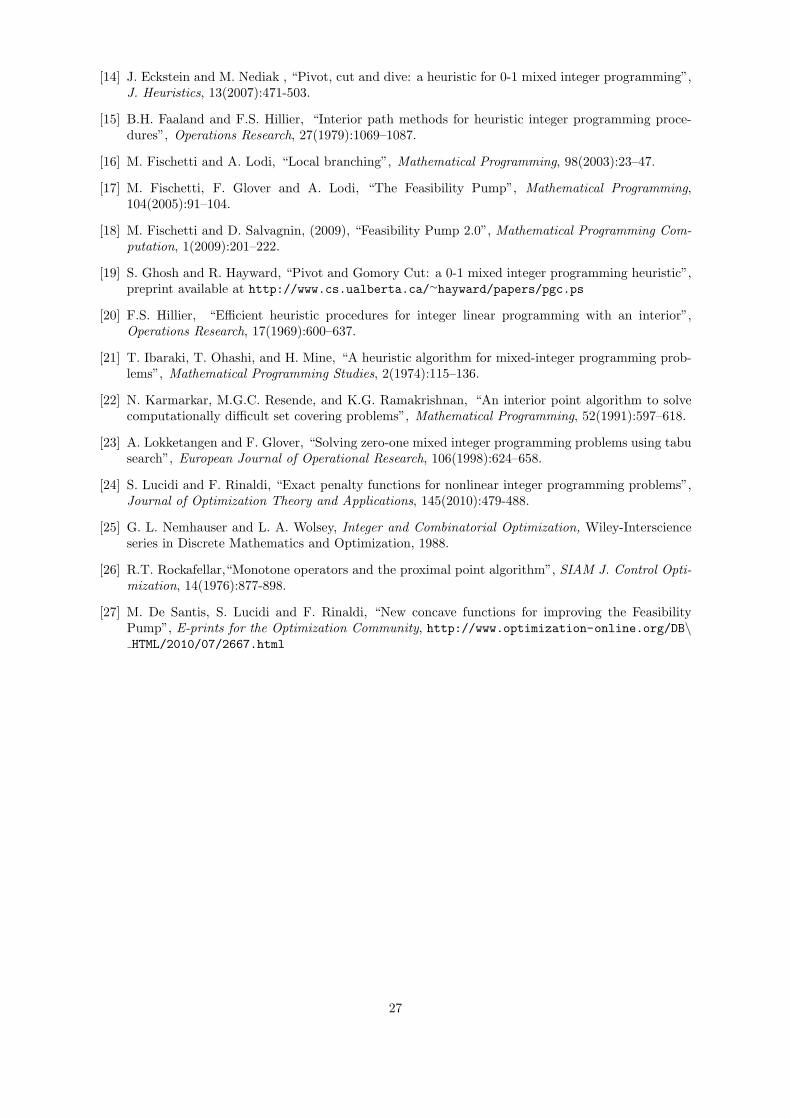
[14] J. Eckstein and M. Nediak , “Pivot, cut and dive: a heuristic for 0-1 mixed integer programming”,J. Heuristics, 13(2007):471-503.

[15] B.H. Faaland and F.S. Hillier, “Interior path methods for heuristic integer programming proce-dures”, Operations Research, 27(1979):1069–1087.

[16] M. Fischetti and A. Lodi, “Local branching”, Mathematical Programming, 98(2003):23–47.

[17] M. Fischetti, F. Glover and A. Lodi, “The Feasibility Pump”, Mathematical Programming,104(2005):91–104.

[18] M. Fischetti and D. Salvagnin, (2009), “Feasibility Pump 2.0”, Mathematical Programming Com-putation, 1(2009):201–222.

[19] S. Ghosh and R. Hayward, “Pivot and Gomory Cut: a 0-1 mixed integer programming heuristic”,preprint available at http://www.cs.ualberta.ca/∼hayward/papers/pgc.ps

[20] F.S. Hillier, “Efficient heuristic procedures for integer linear programming with an interior”,Operations Research, 17(1969):600–637.

[21] T. Ibaraki, T. Ohashi, and H. Mine, “A heuristic algorithm for mixed-integer programming prob-lems”, Mathematical Programming Studies, 2(1974):115–136.

[22] N. Karmarkar, M.G.C. Resende, and K.G. Ramakrishnan, “An interior point algorithm to solvecomputationally difficult set covering problems”, Mathematical Programming, 52(1991):597–618.

[23] A. Lokketangen and F. Glover, “Solving zero-one mixed integer programming problems using tabusearch”, European Journal of Operational Research, 106(1998):624–658.

[24] S. Lucidi and F. Rinaldi, “Exact penalty functions for nonlinear integer programming problems”,Journal of Optimization Theory and Applications, 145(2010):479-488.

[25] G. L. Nemhauser and L. A. Wolsey, Integer and Combinatorial Optimization, Wiley-Interscienceseries in Discrete Mathematics and Optimization, 1988.

[26] R.T. Rockafellar,“Monotone operators and the proximal point algorithm”, SIAM J. Control Opti-mization, 14(1976):877-898.

[27] M. De Santis, S. Lucidi and F. Rinaldi, “New concave functions for improving the FeasibilityPump”, E-prints for the Optimization Community, http://www.optimization-online.org/DB\HTML/2010/07/2667.html

27