a new deep generative network for unsupervised …...6792 ieee transactions on geoscience and remote...

6792 IEEE TRANSACTIONS ON GEOSCIENCE AND REMOTE SENSING, VOL. 56, NO. 11, NOVEMBER 2018

A New Deep Generative Network for UnsupervisedRemote Sensing Single-Image Super-Resolution

Juan Mario Haut , Student Member, IEEE, Ruben Fernandez-Beltran ,Mercedes E. Paoletti , Student Member, IEEE, Javier Plaza , Senior Member, IEEE,

Antonio Plaza , Fellow, IEEE, and Filiberto Pla

Abstract— Super-resolution (SR) brings an excellent oppor-tunity to improve a wide range of different remote sensingapplications. SR techniques are concerned about increasing theimage resolution while providing finer spatial details than thosecaptured by the original acquisition instrument. Therefore, SRtechniques are particularly useful to cope with the increasingdemand remote sensing imaging applications requiring finespatial resolution. Even though different machine learning par-adigms have been successfully applied in SR, more researchis required to improve the SR process without the need ofexternal high-resolution (HR) training examples. This paperproposes a new convolutional generator model to super-resolvelow-resolution (LR) remote sensing data from an unsupervisedperspective. That is, the proposed generative network is able toinitially learn relationships between the LR and HR domainsthroughout several convolutional, downsampling, batch normal-ization, and activation layers. Then, the data are symmetricallyprojected to the target resolution while guaranteeing a recon-struction constraint over the LR input image. An experimentalcomparison is conducted using 12 different unsupervised SRmethods over different test images. Our experiments reveal thepotential of the proposed approach to improve the resolution ofremote sensing imagery.

Index Terms— Convolutional neural networks (CNNs), remotesensing, super-resolution (SR).

Manuscript received February 20, 2018; revised April 12, 2018; acceptedMay 30, 2018. Date of publication June 29, 2018; date of current versionOctober 25, 2018. This work was supported in part by the Ministerio deEducación (resolución de 26 de diciembre de 2014 y de 19 de noviembre de2015, de la Secretaría de Estado de Educación, Formación Profesional y Uni-versidades, por la que se convocan ayudas para la formación de profesoradouniversitario, de los subprogramas de Formación y de Movilidad incluidosen el Programa Estatal de Promoción del Talento y su Empleabilidad, en elmarco del Plan Estatal de Investigación Científica y Técnica y de Innovación2013–2016), in part by the Junta de Extremadura (decreto 297/2014, ayudaspara la realización de actividades de investigación y desarrollo tecnológico,de divulgación y de transferencia de conocimiento por los Grupos de Inves-tigación de Extremadura) under Grant GR15005, in part by the GeneralitatValenciana under Contract APOSTD/2017/007, and in part by the SpanishMinistry of Economy under Project ESP2016-79503-C2-2-P. (Correspondingauthor: Juan Mario Haut.)

J. M. Haut, M. E. Paoletti, J. Plaza, and A. Plaza are with the HyperspectralComputing Laboratory, Department of Technology of Computers and Commu-nications, Escuela Politécnica, University of Extremadura, PC-10003 Cáceres,Spain (e-mail: [email protected]; [email protected]; [email protected];[email protected]).

R. Fernandez-Beltran and F. Pla are with the Institute of New ImagingTechnologies, University Jaume I, 12071 Castellón de la Plana, Spain (e-mail:[email protected]; [email protected]).

Color versions of one or more of the figures in this paper are availableonline at http://ieeexplore.ieee.org.

Digital Object Identifier 10.1109/TGRS.2018.2843525

I. INTRODUCTION

REMOTE sensing image acquisition technology is underconstant development and now provides improved

imagery that are useful to tackle new challenges and needs [1].Nonetheless, the increasing demand of highly accurate remotesensing imaging applications, such as fine-grained classifica-tion [2], [3], target recognition [4], [5], object tracking [6], [7],and detailed land monitoring [8], still makes the spatial reso-lution of optical sensors one of the most important limitationsaffecting remotely sensed imagery. In general, the spatialresolution of an instrument defines the pixel size coveringthe Earth surface, and, therefore, it describes the ability ofthe sensor to capture small image details. Even though themost technologically advanced satellites are able to discernspatial information within a squared meter on the Earthsurface [9], the high cost of this acquisition technology,together with the light physical limitations when substan-tially decreasing the sensor pixel size, is usually importantconstraints that make algorithmic-based resolution enhance-ment techniques an excellent tool for remote sensing imagingapplications [10].

The general objective in super-resolution (SR) [11]–[14]is to improve the image resolution beyond the sensor limits,that is, increasing the number of image pixels while providingfiner spatial details than those captured by the original acqui-sition instrument. Depending on the number of input images,it is possible to distinguish between two kinds of SR methods,single-image [15] and multi-image [16]. Single-image SRtechniques use a single image of the target scene to obtainthe super-resolved output, whereas multi-image SR methodsrequire several scene shots simultaneously acquired at differentpositions. In remote sensing, the single-image approach isusually adopted, because it provides a more general schemeto super-resolve any kind of imaging sensor without the needfor a satellite constellation [17], [18].

The single-image SR approach can be considered as an ill-posed problem, since there is not a single solution for anygiven low-resolution (LR) pixel, i.e., the solution is not unique.This fact has been traditionally mitigated by constraining thespace of possible solutions using a strong prior informationextracted from a specific set of images. In this sense, artificialneural networks (ANNs) have become a powerful tool due totheir ability to learn image priors from any given data set.Traditionally used in the pattern recognition field [19], ANNs

0196-2892 © 2018 IEEE. Personal use is permitted, but republication/redistribution requires IEEE permission.See http://www.ieee.org/publications_standards/publications/rights/index.html for more information.

https://orcid.org/0000-0001-6701-961X

https://orcid.org/0000-0003-1374-8416

https://orcid.org/0000-0003-1030-3729

https://orcid.org/0000-0002-2384-9141

https://orcid.org/0000-0002-9613-1659

HAUT et al.: NEW DEEP GENERATIVE NETWORK FOR UNSUPERVISED REMOTE SENSING SINGLE-IMAGE SR 6793

have also been intensively used for the analysis of remotelysensed imagery [20]–[22], reaching a good performancewithout prior knowledge on the input data distribution andoffering multiple training techniques.

With the great evolution of deep learning [23], [24] (DL)techniques, the ANN architecture has evolved from the simplelinear perceptron classifier to deeper architectures (multilayerstack of simple modules) called deep neural networks (DNNs),allowing to create more complex models which can extractmore abstract information (features) from the data than shallowones [25]. DNNs are currently able to perform SR in asuccessfully way [26]. In particular, convolutional neural net-works (CNNs) [23] stand out as a powerful image processingtool due their effectiveness, especially for the analysis oflarge sets of 2-D images. CNNs have proven to produce highperformance in a great variety of tasks, such as image analysisand target detection [27]–[30], pan-sharpening [31], [32],reconstruction of remote sensing imagery [33], and also imageSR [34]–[38]. However, these supervised techniques requiresufficient high-resolution (HR) training examples in order toperform properly and generalize well. In addition, they usuallytend to overfit quickly due to the models’ complexity andthe lack of training data. Note that obtaining the relevantremote sensing training data is expensive and time-consuming.Besides, the number of available training remote sensingdata sets is rather limited, and normally, they suffer froma lack of image variations and diversity. For these reasons,supervised learning is difficult to carry out, while unsupervisedlearning methods do not need any external data to train.On the other hand, the CNN is a very flexible model thatcan be adapted to different learning models, such as con-volutional autoencoders [39], [40], convolutional deep beliefnetworks [41], convolutional generative adversarial neural net-works [42], convolutional recurrent neural networks [43], andfully convolutional networks [44], among others. In particular,we highlight the hourglass network [45], [46], whose topologyis symmetric, related to the convolution–deconvolution archi-tecture and also to the encoder–decoder, characterized by afirst step of pooling down to a lower resolution (composedof convolutional and max pooling layers) and a second stepof upsampling to a higher resolution and combining featuresacross multiple resolutions.

Following the hourglass approach, a new unsupervisedneural network model is proposed in this paper in orderto super-resolve remote sensing images. The novelty of theproposed approach lies on using a generative random noiseto introduce a higher variety of spatial patterns, which can bepromoted to a higher scale throughout the network accord-ing to a global reconstruction constraint. Even though therelevance of generating new spatial variations when super-resolving remotely sensed data in an unsupervised manner, thisis, to the best of our knowledge, the first time an unsupervisedgenerative network model has been successfully formulated tosuper-resolve remote sensing imagery. Specifically, a convo-lutional generator network has been adopted, where from agiven image XLR ∈ R

C×W×H , a higher resolution versionXHR ∈ R

C×t ·W×t ·H is generated (where W < t · W andH < t · H , with t being a factor of resolution).

In addition, the algorithm has been adapted to be efficientlyexecuted in parallel on graphics processing units (GPUs)1

and presents some methodological improvements to make themodel more efficient and effective. To summarize, the maincontributions of this paper can be highlighted as follows.

1) An hourglass CNN model is developed to performunsupervised SR.

2) In particular, a convolutional generator model hasbeen implemented to super-resolve LR remote sensingimages.

3) Starting from generative random noise, the model is ableto reconstruct the image, promoting it to a higher scaleaccording to a global reconstruction constraint.

4) Experiments over three data sets, with two scalingfactors and 12 different SR methods, reveal the compet-itive performance of the proposed model when super-resolving remotely sensed images.

The remainder of this paper is organized as follows.Section II presents an overview of single-image SR methodsand their limitations. Section III describes the methodol-ogy used by the proposed convolutional generator model.Section IV validates the proposed approach by performingcomparisons with different single-image SR methods. Finally,Section V concludes this paper with some remarks and hintsat plausible future research lines.

II. BACKGROUND

A. Brief Single-Image SR Overview

Broadly speaking, single-image SR algorithms can be cat-egorized into three different groups [53], [54]: image recon-struction (RE), image learning (LE), and hybrid (HY) methods.RE methods aim at reconstructing HR details in the super-resolved output assuming a specific degradation model alongthe image acquisition process, which is typically defined bythe concatenation of three operators: blurring, decimation,and noise. Therefore, RE methods can be usually defined interms of the three following stages (see Fig. 1): Stage 1,where the LR input image (ILR) is upscaled to the targetresolution (ILRI) using a regular interpolation kernel function.In Stage 2, some physical features are extracted from ILRto estimate the singularities of the spatial details. Finally,Stage 3 aggregates both the interpolated image (ILRI) andthe extracted LR features to obtain the final reconstructedresult ISR.

Each particular RE method makes its own assumptionsabout the imaging model and the reconstruction process torelieve the ill-posed nature of the SR problem. Some ofthe most popular RE approaches are iterative back projec-tion (IBP) [55], gradient profile prior (GPP) [56], and pointspread function (PSF) deconvolution [57]–[59]. The rationalebehind IBP is based on iteratively refining an initial interpo-lation result by means of minimizing the reconstruction errorbetween the LR input image and a simulated LR version of the

1The use of high-performance computing methods, including parallelizationwith accelerators such as field-programmable gate arrays and GPUs [47]–[49], or the distribution with clusters and clouds [50], [51], has demonstratedgreat utility for the classification of remote images [52].


Fig. 1. SR based on image reconstruction (RE).

Fig. 2. SR based on image learning (LE).

super-resolved result. GP takes advantage of the fact that theshape of the gradient profiles tends to remain invariant acrossscales, and therefore, LR gradient can be used to reconstructthe output image sharpness. PSF deconvolution methods tacklethe upscaling problem from a deblurring point of view, that is,they initially estimate the imaging model PSF and then theytry to remove the interpolated image blur.

Regarding LE methods, this type of techniques are able toprovide a more powerful SR scheme, because they learn therelationships between LR and HR domains from an externaltraining set containing ground-truth HR images. As shownin Fig. 2, RE methods can be divided into three stages:in Stage 1, the relations between LR and HR componentsare learned from a specific training set. Stage 2 aims atestimating the HR components that are related to the LRinput image structures. Finally, Stage 3 combines the estimatedHR components to generate the final super-resolved result.Over the past years, different machine learning paradigmshave been successfully applied in LE-based SR. Sparse cod-ing [60], neighborhood embedding [61], and mapping func-tions [62], [63] are among the most popular methods. In anutshell, sparse coding-based techniques take advantage ofthe fact that natural images tend to be sparse when theyare characterized as a linear combination of small patches.The neighborhood embedding approach assumes that smallimage patches of LR images describe a low-dimensionalnonlinear manifold with a similar local geometry to their HRcounterparts. Mapping-based techniques cope with the SR taskas a regression problem between the HR and LR domains.

Finally, HY techniques work toward reaching an agreementbetween the RE and LE approaches. In particular, they per-form a training process but only using the LR input image.The rationale behind the HY methods is based on the patch

Fig. 3. SR based on HY algorithms.

redundancy property pervading natural images, which assumesthat natural images tend to contain repetitive structures withinthe same scale and over scales as well. Taking this principleinto account, it is possible to find patches which appearin a lower scale, without any blurring or decimation, andthen extracting their corresponding HR counterparts from thehigher scale image. Eventually, the super-resolved image canbe generated using the LR/HR relationships learned acrossscales. In particular, HY methods generally follow the schemeshown in Fig. 3: in Stage 1, the self-learning process isconducted, that is, several lower scale images are initiallygenerated from ILR and then those patches which tend toappear across scales are extracted. Stage 2 projects the inputLR image to the target resolution using the relations previouslylearned. Finally, the final super-resolved result is generated inStage 3 considering some sort of reconstruction constraint.

Logically, each specific HY approach defines its ownassumptions about the imaging model and the patch searchingcriteria. For example, the work presented in [64] approxi-mates the blur operator by a Gaussian kernel, and the patchredundancy process is conducted by an approximation of thenearest neighbor search. Other works propose different kindsof modifications over this scheme. It is the case of [65],which introduces a model extension to enable patch geometrictransformations across scales. Therefore, the number of patchmatches can be increased and consequently the amount oflearned LR/HR relationships. In other works, such as in [66],the blur operator is estimated at the same time as the SR outputis generated through an optimization process.

B. SR Limitations in Remote Sensing

Each single-image SR methodology has shown to be partic-ularly effective under specific conditions [15], [54]. RE meth-ods are able to reduce the noise as well as the blur andaliasing inherent to interpolation kernel functions. However,the lack of relevant high-frequency information in the LR inputimage limits their effectiveness to small magnification factors,which can be an important limitation for many of the currentlyoperational (moderate) resolution satellites [67].

LE-based techniques potentially overcome these drawbacksby learning the relationships between LR and HR domainsfrom an external training set. Nonetheless, the availability ofsuitable HR training examples can also be a serious constraint


for many satellites. Note that the ground-truth HR images areusually not available in real scenarios, and this may lead to anunrepresentative training phase with a biased super-resolvedresult. Eventually, the application of LE-based SR methodsin actual ground segment production environments is ratherlimited [68].

HY methods offer the advantage of not requiring anyexternal training set to learn the LR/HR relationships bytaking advantage of the patch redundancy property over scales.However, the probability of finding patches satisfying thisproperty decreases with the input resolution, and therefore,the amount of useful LR/HR connections over scales highlydepends on the input image.

With all these considerations in mind, unsupervised REand HY methods are especially attractive to remote sens-ing. While supervised approaches use a training set of HRimages to learn the relationships between the LR and HRdomains [35], [69], [70], unsupervised approaches only makeuse of the target LR image to generate the correspondingsuper-resolved output result. Moreover, supervised networkarchitectures implement a regressor function to project generalLR image patches onto the HR domain. However, in a real-life remotely sensed data production environment, there is noactual HR captured by the sensor. In this sense, unsupervisedmethods do not require the availability of HR images to traina general SR model, super-resolving each specific LR inputimage without using any other external data and providingthe opportunity to offer new super-resolved data products insatellite and airborne missions that use relatively inexpensivesensors without the need of using any external HR trainingset. Nevertheless, the number of works in the remote sensingliterature dealing with the unsupervised SR problem is ratherconstrained, and this is precisely the gap that motivates thispaper.

Mianji et al. [71] proposed an SR approach using abackpropagation neural network as a regression function andbasing on: 1) spectral unmixing; 2) SR mapping; and 3) self-training, which is exploited taking advantage of the embeddingprovided by the spectral unmixing process itself. However,this approach could be highly affected by the spectral simplexgeometry of the input image [72]. In contrast, an HY (alsocalled self-learning) SR scheme has been proposed in thispaper to super-resolve remote sensing data from an unsuper-vised perspective, basing on a new end-to-end convolutionalgenerator model. The rationale behind the proposed approachis based on learning the relationships between the LR andHR domains by downsampling the original input image to alower scale and then using the learned relations at a lowerscale to project the LR input image to the target resolution.However, the amount of spatial information that it is possibleto retrieve from a downsampled LR image may be limited,so a random generative noise has been additionally introducetogether with a global reconstruction constraint to activate ahigher amount of consistent spatial variations along the SRprocess. That means, random spatial variations are initiallygenerated to be introduced in the self-learning process inorder to mitigate the ill-posed nature of the SR problem.Regarding the proposed network global scheme, it provides

a similar end-to-end framework to other DL-based approaches,e.g., [35], [69], [70], where the original LR image is used tolearn the downsampling filters at the same time that they arealso used to generate the super-resolved output.

III. METHODOLOGY

Traditionally, a generator network is an algorithm for imagegeneration, where given a random variable z, the model is ableto learn internal relationships (represented by the model para-meters θ ) to generate an image X = fθ (z), i.e., a regressionproblem. This allows us to learn the distribution of the dataand the correlations between z and X . We can follow thisapproach in order to perform SR over remote sensing images,where z ∈ R

C×W×H is a random noise and X ∈ R3×W �×H � is

the desired RGB HR image.Given an LR image XLR ∈ R

3×W×H , the SR’s goal isto improve the image resolution beyond the sensor limitsobtaining an HR version XHR ∈ R

3×t ·W×t ·H from XLR, wheret is the resolution factor and W < t ·W , H < t ·H . In order todo this, a deep model based on CNNs has been implemented.This kind of networks is composed of the layers that areapplied over defined regions of the input data, i.e., they arelocally connected to the input, transforming the input volumeto an output volume of neuron activations which will serveas an input to the next layer. The fact that each layer isnot completely connected to the previous layer (only witha patch/window defined as the receptive field) is a greatadvantage for data analysis, thus reducing the number ofconnections in the network, where each layer composes featureextraction stages working as a filter or kernel over patches ofthe input volume.

Depending on the treatment of the data, CNNs can beclassified into three categories. Supposing that x (i) ∈ R

C =[x (i)

1 , x (i)2 , . . . , x (i)

C ] is a pixel with C spectral bands of imageX ∈ R

C×W×H , with i = 1, 2, . . . , W · H , while P( j ) ∈R

b×p×p is a patch of X , where p is the width and height (withp ≤ W and p ≤ H ) and b is the number of spectral bandsof the patch (with b ≤ C). 1-D-CNN models take separatelyas input data each pixels vector x (i), extracting only spec-tral information [73]. On the other hand, 2-D-CNNs extractspatial information, taking as input data the entire imageX [74] or image patches P( j ) [75], where C and b are set tosmall values, i.e., the spectral information is not very relevantcompared with the spatial information. Finally, 3-D-CNNsextract spectral–spatial information, taking normally as inputdata patches P( j ) of the original image X [29], [30], whereC and b are set to large values, i.e., the spectral informationis very relevant and it is combined with spatial information.Usually, for panchromatic and RGB remote sensing images,a 2-D-CNN approach is taken, while 1-D- and 3-D-CNNs areusually for multispectral and hyperspectral images. This paperworks with the RGB remote sensing data sets, so the 2-D-CNN architecture has been implemented to take advantage ofthe spatial information contained in the images. It is composedof five different kinds of layers, as described in the following.

1) Convolution (CONV) Layer: This kind of layer is com-posed of a block of neurons where each slice (also called


a filter or a kernel) shares its weights and biases betweenall the neurons that compose it. Given a CONV layerC(i), its output volume O(i) (also called feature maps)can be calculated by the following (1) as the dot productbetween the n(i) slices’ weights W (i) and biases B(i)

(where n(i) is the number of depth slices, also known asnumber of filters or kernels) and a small region of theinput volume O(i−1), i.e., a rectangular section of theprevious layer C(i−1), defined by the kernel size k(i) ofthe current layer C(i):

O(i) = (O(i−1) · W (i)) f,l + B(i)

=k(i)�

m=1

k(i)�n=1

(o(i−1)f−m,l−n · w(i)

m,n)+ B(i) (1)

where o(i−1)f,l is the feature ( f, l) of the feature map

O(i−1) ∈ RW,H , with f = 1, 2, . . . , W and l =

1, 2, . . . , H , and w(i)m,n is the weight (m, n) of the weight

matrix W (i) ∈ Rk(i),k(i)

. As a result, O(i) ∈ Rn(i),W �,H �

forms a data cube whose depth is defined by the numberof kernels n(i) (that indicates the number of outputfeature maps) and its width and height are calculated as

W � = (Wk + 2P)

S+ 1 and H � = (H k + 2P)

S+ 1

respectively, where P indicates the padding (zeros)added to the input data borders and S indicates the strideof the kernel over the data. W and H are, respectively,the width and height of the previous feature mapsO(i−1) ∈ R

n(i−1),W,H .2) Batch Normalization (BATCH-NORM) Layer: Normally,

it is placed behind the convolution layer, and it appliesthe normalization defined by (2) over the batch data

y = x −mean[x]√Var[x] + �

· γ + β (2)

where γ and β are the learnable parameter vectors, and� is a parameter for numerical stability.

3) Activation Layer: After CONV and BATCH-NORMlayers, the activation layer or the nonlinearity layerembeds a nonlinear function that is applied over theoutput of the previous layer as the rectified linearunit (ReLU) [76], [77]. In this case, the LeakyReLUfunction is implemented [78]

f (x) =�

x if x > 0

αx if x ≤ 0(3)

where α is a small nonzero parameter, normally 0.001.4) Downsampling/Upsampling Layer: The proposed model

also implements downsampling and upsampling layersat certain locations of the architecture. The first onereduces the spatial resolution of the input volumes byreducing the width and height with a resolution fac-tor t . A max pool function is generally implemented toperform the downsampling, and however, the proposedmodel downsamples the input data setting the strides of

certain CONV layers to S = 2. In addition, the upsam-pling layers try to reconstruct the data size using thebilinear function given a scaling factor.

The proposed methodology provides a novel approach toeffectively super-resolve remote sensing data from an unsuper-vised perspective. Specifically, our model receives the randomnoise vector z as input data, which is resized into a cubematrix R

C×t ·W×t ·H in order to feed the network, where Wand H are the width and height of the original LR remotesensing image, C = 3 is the number of spectral channels,and t is the resolution factor. Following a fully connectedhourglass architecture [45], [79], z goes through two mainsteps composed of several blocks as follows.

1) The downsampling step is composed of N blocks oflayers, called d(i) (i = 1, 2, . . . , N), where the input ofeach one is the feature maps of the previous one. Eachd(i) is composed of an initial CONV layer C(1)

d thatperforms the downsampling step by its stride S = 2,dividing the output volume size by two. This outputvolume feeds the BATCH-NORM layer and the non-linear LeakyReLU activation function. The output ofthe neuron activations feeds the second CONV layerC(2)

d without downsampling (i.e., S = 1) and alsofollowed by a BATCH-NORM layer and the LeakyReLUactivation function. C(1)

d and C(2)d have their own number

of filters (n(1)d and n(2)

d ) and their own kernel size

(k(1)d and k(2)

d ). In fact, each block d(i) is reducingthe space information, i.e., generating a low spatialresolution data that will feed the second upsamplingstep.

2) The upsampling step is symmetric to downsampling one,and it is also composed of N blocks of layers, calledu(i) (i = N, . . . , 2, 1), where the input of each oneis the output of the previous one. In this case, eachu(i) is composed of several stacked layers. The firstone is a BATCH-NORM layer, followed by the firstCONV layer C(1)

u (which maintains the size of the data,i.e., S = 1) and its BATCH-NORM and LeakyReLUfunction. The output of the neuron activations feedsthe second convolutional layer C(2)

u (which also main-tains the size of the data). After the BATCH-NORMand the activation function, the output will finally feedthe bilinear upsampling layer with factor equal to 2.Again, C(1)

u and C(2)u have their own number of filters

(n(1)u and n(2)

u ) and their own kernel size (k(1)u and k(2)

u ).Both the steps, downsampling and upsampling, are symmetri-cal and connected by skip connections, i.e., the input of eachupsampling block u(i) is combined with the corresponding d(i)

through the skip connection s(i) (i = 1, 2 . . . , N) composedof a CONV layer C(1)

s , with its number of filters n(i)s and its

kernel size k(i)s , a BATCH-NORM layer, and the activation

function, LeakyReLU. In fact, the output of s(i) is concate-nated to the input of u(i). The chosen topology is shownin Fig. 4. At the end of the topology, an output block is added,composed of a CONV layer and a sigmoid function at the end.As a result, an HR image XHR

o ∈ R3×t ·W×t ·H is generated as

an output of the network.


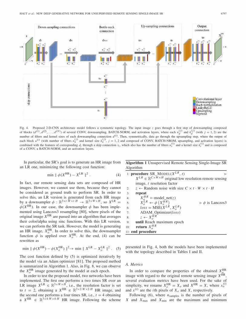
Fig. 4. Proposed 2-D-CNN architecture model follows a symmetric topology. The input image z goes through a first step of downsampling composedof blocks (d(1), d(2), . . . , d(N )) of several CONV, downsampling, BATCH-NORM, and activation layers, where each n( j )

d and k( j )d (with j = 1, 2) are the

number of filters and kernel sizes of each downsampling connection d(i) . Then, symmetrically, data go through the upsampling step, where the output ofeach block u(i) (with number of filters n( j )

u and kernel size k( j )u , j = 1, 2 and composed of CONV, BATCH-NROM, upsampling, and activation layers) is

combined with the features of corresponding di through a skip connection si , which also has the number of filters n(1)s and a kernel size k(1)

s and is composedof a CONV, a BATCH-NORM, and an activation layers.

In particular, the SR’s goal is to generate an HR image froman LR one, minimizing the following cost function:

min � φ(XHR)− XLR �2 . (4)

In fact, our remote sensing data sets are composed of HRimages. However, we cannot use them, because they cannotbe considered as ground truth to perform SR. In order tosolve this, an LR version is generated from each HR imageby a downsampler φ : R

3×t ·W×t ·H → R3×W×H , so XLR =

φ(XHR). In our case, the downsampler φ has been imple-mented using Lanczos3 resampling [80], where pixels of theoriginal image XHR are passed into an algorithm that averagestheir color/alpha using sinc functions. With this LR version,we can perform the SR task. However, the model is generatingan HR image, XHR

o . In order to solve this, the downsamplerfunction φ is applied over XHR

o . At the end, (4) can berewritten as

min � φ(XHR)− φ(XHRo ) �2→ min � XLR − XLR

o �2 . (5)

The cost function defined by (5) is optimized iteratively bythe model via an Adam optimizer [81]. The proposed methodis summarized in Algorithm 1. Also, in Fig. 8, we can observethe XHR

o image generated by the model at each epoch.In order to test the proposed model, two networks have been

implemented. The first one performs a two times SR over anLR image XLR ∈ R

3×W×H , i.e., the resolution factor is setto t = 2, obtaining a XHR ∈ R

3×2·W×2·H HR image, andthe second one performs a four times SR, i.e., t = 4 obtaininga XHR ∈ R

3×4·W×4·H HR image. Following the scheme

Algorithm 1 Unsupervised Remote Sensing Single-Image SRAlgorithm

1: procedure SR_MODEL(X L R , t) �X L R ∈ R

C×W×H original low resolution remote sensingimage, t resolution factor

2: z← Random noise with size C × t ·W × t · H3: repeat4: X H R

o ←model_net(z)5: X L R

o ← φ�

X H Ro

� � φ is Lanczos36: loss = MSE(X L R, X L R

o )7: ADAM_Optimizer(loss)8: z← X H R

o9: until Reach maximum epoch

10: return X H Ro

11: end procedure

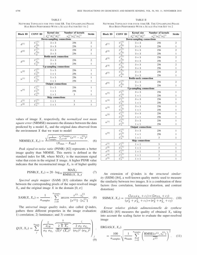
presented in Fig. 4, both the models have been implementedwith the topology described in Tables I and II.

A. Metrics

In order to compare the properties of the obtained XHRo

image with regard to the original remote sensing image XHR,several evaluation metrics have been used. For the sake ofsimplicity, we rename XHR

o = Xo and XHR = X , where x (i)o

and x (i) are the i th pixels of Xo and X , respectively.Following (6), where nsamples is the number of pixels of

X and Xmax and Xmin are the maximum and minimum


TABLE I

NETWORK TOPOLOGY FOR TWO-TIME SR. THE UPSAMPLING PHASEHAS BEEN PERFORMED WITH A SCALE-FACTOR SET TO 2

values of image X , respectively, the normalized root meansquare error (NRMSE) measures the distance between the datapredicted by a model Xo and the original data observed fromthe environment X that we want to model

NRMSE(X, Xo) =�

1nsamples

·�nsamplesi=0 (x (i) − x (i)

o )2

(Xmax − Xmin). (6)

Peak signal-to-noise ratio (PSNR) [82] represents a betterimage quality than NRMSE. This metric is defined as thestandard index for SR, where MAX f is the maximum signalvalue that exists in the original X image. A higher PSNR valueindicates that the reconstructed image Xo is of higher quality

PSNR(X, Xo) = 20 · log10MAX f

RMSE(X, Xo). (7)

Spectral angle mapper (SAM) [83] calculates the anglebetween the corresponding pixels of the super-resolved imageXo and the original image X in the domain [0, π]

SAM(X, Xo) = 1

nsamples·

nsamples�i=0

arccosx (i) · x (i)

o

�x (i)� · �x (i)o �

. (8)

The universal image quality index, also called Q-index,gathers three different properties in the image evaluation:1) correlation; 2) luminance; and 3) contrast

Q(X, Xo) =nbands�

j

⎛⎜⎜⎜⎝

a� � �σI R

σX σXo

b� � �2 X Xo

(X)2 (Xo)2

c� � �2 σX σXo

(σX )2 (σXo)2

⎞⎟⎟⎟⎠

j

.

(9)

TABLE II

NETWORK TOPOLOGY FOR FOUR-TIME SR. THE UPSAMPLING PHASEHAS BEEN PERFORMED WITH A SCALE-FACTOR SET TO 2

An extension of Q-index is the structural similar-ity (SSIM) [84], a well-known quality metric used to measurethe similarity between two images. It is a combination of threefactors (loss correlation, luminance distortion, and contrastdistortion)

SSIM(X, Xo) = (2μXμXo + c1) ∗ (2σX Xo + c2)

(μ2X + μ2

Xo+ c1) ∗ (σ 2

X + σ 2Xo+ c2)

. (10)

Erreur relative globale adimensionnelle de synthese(ERGAS) [85] measures the quality of obtained Xo takinginto account the scaling factor to evaluate the super-resolvedimage

ERGAS(X, Xo)

= 100

nsamples

�� 1

nbands

nsamples�i=0

�RMSE(x (i), x (i)

o )

x (i)

�2

. (11)


IV. EXPERIMENTS

A. Experimental Configuration and Data Sets

In order to test the performance of the proposed model,several experiments have been conducted using two differenthardware environments as follows.

1) A GPU environment composed of a sixth GenerationIntel Core i7-6700K processor with 8 M of Cache andup to 4.20 GHz (4 cores/8-way multitask processing),40 GB of DDR4 RAM with a serial speed of 2400 MHz,a GPU NVIDIA GeForce GTX 1080 with 8-GBGDDR5X of video memory and 10 Gb/s of memoryfrequency, a Toshiba DT01ACA HDD with 7200 rpmand 2 TB of capacity, and an ASUS Z170 pro-gamingmotherboard. The software environment is composed ofUbuntu 16.04.4 x64 as an operating system, Pytorch [86]0.3.0, and compute device unified architecture (CUDA)8 for GPU functionality.

2) A CPU environment composed of Intel Core i7-4790 @3.60 GHz, 16 GB of DDR3 RAM with a serial speedof 800 MHz, and a Western Digital HDD with 7200 rpmand 1 TB of capacity. The software environment iscomposed of Windows 7 as an operating system andMATLAB R2013a.

It should be noted that our proposed method has been exe-cuted on the GPU environment, while the other methods havebeen executed in the CPU environment. Although our methoduses Pytorch and CUDA, its parallelization can still be furtheroptimized, and therefore, the difference in computation timeswith regard to the other methods was not very significant.

In addition, the employed database is composed of multipleRGB images from three different remote sensing repositorieswith the aim of testing the SR approach process under differentsensor’s acquisition conditions and including different kinds ofsmall perturbations. No additional levels of noise have beenconsidered due to the design of the proposed SR approach,given by the noise-free scheme of (4), presented in otherapproaches, such as [35], [69], [70] and [87]. The employedrepositories are described in the following and are publiclyavailable on this repository (see Fig. 5).2

1) UCMERCED [88]: It is composed of 21 land-useclasses, including agricultural, airplane, baseball dia-mond, beach, buildings, chaparral, dense residential,forest, freeway, golf course, harbor, intersection, mediumdensity residential, mobile home park, overpass, parkinglot, river, runway, sparse residential, storage tanks, andtennis courts images. Each class consists of 100 imageswith 256× 256 pixels and a pixel resolution of 30.

2) RSCNN7 [89]: This data set contains 2800 imageswith seven different classes. The data set is ratherchallenging due to the wide differences of the scenes,which have been captured under changing seasons andvarying weathers and sampled with different scales. Theresolution of individual images is 400× 400 pixels.

3) NWPU-RESIS45 [90]: The remote sensing image sceneclassification data set has been created by NorthwesternPolytechnical University. This data set has 45 scenes

2https://github.com/mhaut/images-superresolution

Fig. 5. Data set used in the experiments, comprising the following images:agricultural, agricultural2, airplane, baseball, bridge, circular-farmland, harbor,industry, intersection, parking, residential, and road.

TABLE III

METHODS CONSIDERED FOR THE EXPERIMENTS. FURTHER DETAILSCAN BE FOUND IN THE CORRESPONDING REFERENCES

with a total number of 31500 images, 700 per class.The size of each image is 256× 256 pixels.

From these images, an LR version has been generated fromtheir corresponding HR counterparts following a two-step pro-cedure [91]: 1) an initial blurring step and 2) a final decimationprocess. In particular, a Lanczos3 windowed sinc filter hasbeen used for blurring the corresponding HR images, andthen, these images have been downsampled according to theconsidered scaling factors (2 and 4, respectively). Regardingthe blurring step, it should be noted that the Lanczos3 kernelsize has been adapted to the scaling factor using the followingexpression, w = (4∗s+1), where w represents the filter widthand s is the considered scaling factor. For the downsamplingprocess, image rows and columns have been selected fromthe top-left corner using a stride equal to the consideredscaling factor. The goal behind this preprocessing step is togenerate LR images from ground-truth HR ones maintainingthe acquisition sensor properties but considering a lowerspatial resolution. In this way, it has been possible to conduct afull-reference assessment protocol in experiments.


TABLE IV

AVERAGE SR RESULTS. THE BEST RESULT FOR SCALING RATIO AND METRIC IS HIGHLIGHTED IN BOLD FONT

The performance of the proposed approach has been com-pared with the results obtained by 11 different unsupervisedSR methods available in the literature, as well as the bicu-bic interpolation kernel function [80] used as an upscalingbaseline. These SR methods have been considered for theexperimental discussion, because they provide an unsupervisedSR scheme in the same way that the proposed approach does,using the LR input image to generate a super-resolved outputresult. In addition, two different scaling factors, two times andfour times, have been tested over the considered image dataset (see Section IV-A). Table III provides a brief descriptionof the SR techniques considered in the experimental part ofthis paper.

All the tested methods have been downloaded from thefollowing website,3 and they have been used consideringthe default settings suggested by the methods’ authors foreach particular scaling ratio [54]. Note that this configurationprovides the most general scenario to super-resolve a widerange of image types taking into account the tested imagediversity.

B. Results

Tables V–VII present the quantitative assessment of theconsidered SR methods in terms of seven different qualitymetrics. Specifically, each table contains the super-resolvedresults of four test images, and for each image, the SR resultsare provided in rows considering two different scaling factors,two times and four times, which are shown in columns.Besides, Table IV provides the average results for the wholeimage collection in order to provide a global view.

In addition to the quantitative evaluation provided by theconsidered metrics, some visual results are provided as aqualitative evaluation for the tested SR methods. Specifi-cally, Figs. 6 and 7 show the super-resolved results obtainedfor harbor and road test images considering two-time andfour-time scaling factors, respectively. Besides, Fig. 8 presentsthe visual evolution of the super-resolved result along thenetwork iterations.

3http://www.vision.uji.es/srtoolbox/

C. Discussion

According to the quantitative assessment reported inTables IV and V, it is possible to rank the global performanceof the tested SR methods into three different categories:1) high performance: for the proposed approach; TSE and SRI,2) moderate performance: for IBP, DLU, DRE, and UMK; and3) low performance: for GPP, LSE, GPR, BDB, and FSR.

When considering a two-time scaling factor, the proposedapproach (together with the HY methods TSE and SRI)provides a significant improvement with respect to the BCIbaseline. Specifically, the proposed approach obtains thebest performance for NRMSE, PSNR, and ERGAS metrics,whereas TSE exhibits the best result for Q-index, SSIM,and SAM. Although TSE and SRI also achieve, on average,a remarkable improvement over the baseline, the proposedapproach provides a more consistent performance, becauseit obtains the best average result for NRMSE, PSNR, andERGAS metrics, and the second best value for Q-index,SSIM, and SAM. It can be observed that the average PSNRgain provided by the proposed approach is 0.39 dB for twotimes and 0.48 dB for four times. Regarding the methodsproviding a moderate improvement 2), the PSF deconvolution-based techniques, DLU, DRE, and UMK, provide a similaraverage performance, and IBP is able to obtain a slightly betterquantitative result over all the considered metrics. Within thelow-performance method group 3), it is possible to see thatGPP and LSE methods provide a result similar to the oneobtained by the baseline, and GPR, BDB, and FSR obtaineven a worse result.

A similar trend can be observed when considering a four-time scaling factor. In this case, the proposed approach is,on average, the best method according to NRMSE, PSNR,and ERGAS metrics. TSE obtains the best Q-index and SSIMresults, and both the methods obtain a similar average resultfor the SAM metric. It should be noted that SRI performancehas worsened when using a four-time ratio, and however, it stillobtains the third best Q-index and SSIM results. With respectto the rest of the moderate 2) and low-performance methods 3),they obtain similar results with regard to the ones obtainedwith a two-time factor. Overall, the proposed approach and


Fig. 6. SR results obtained using the methods shown in captions over the test image harbor with a two-time scaling factor. For each result, PSNR (dB) valuesappear in brackets. The best PSNR value is highlighted in bold. (a) HR. (b) BCI (21.73 dB). (c) IBP (23.43 dB). (d) SRI (25.82 dB). (e) DLU (23.40 dB).(f) UMK (23.44 dB). (g) TSE (25.63 dB). (h) Proposed approach (26.84 dB).

Fig. 7. SR results obtained using the methods shown in captions over the test image road with a four-time scaling factor. For each result, PSNR (dB) valuesappear in brackets. The best PSNR value is highlighted in bold. (a) HR. (b) BCI (20.57 dB). (c) IBP (21.86 dB). (d) SRI (22.36 dB). (e) DLU (21.32 dB).(f) UMK (21.93 dB). (g) TSE (23.86 dB). (h) Proposed approach (25.69 dB).

TSE have shown to obtain the best quantitative performancefollowed some way behind by SRI. However, the differencesamong these methods are relatively small, which motivates athorough discussion over qualitative results to find out eachmethod’s singularity.

According to the visual results presented in Figs. 6 and 7,each SR method tends to foster a particular kind of visual

feature on the super-resolved output. Some methods, likeTSE or SRI, are able to obtain sharper edges, while others,like DLU or UMK, seem more robust to noise by generatingsmoother super-resolved textures. In terms of visual per-ceived quality, the proposed approach achieves a remarkableperformance. For instance, the boat detail in Fig. 6(h) iscertainly the most similar to its HR counterpart in Fig. 6(a).


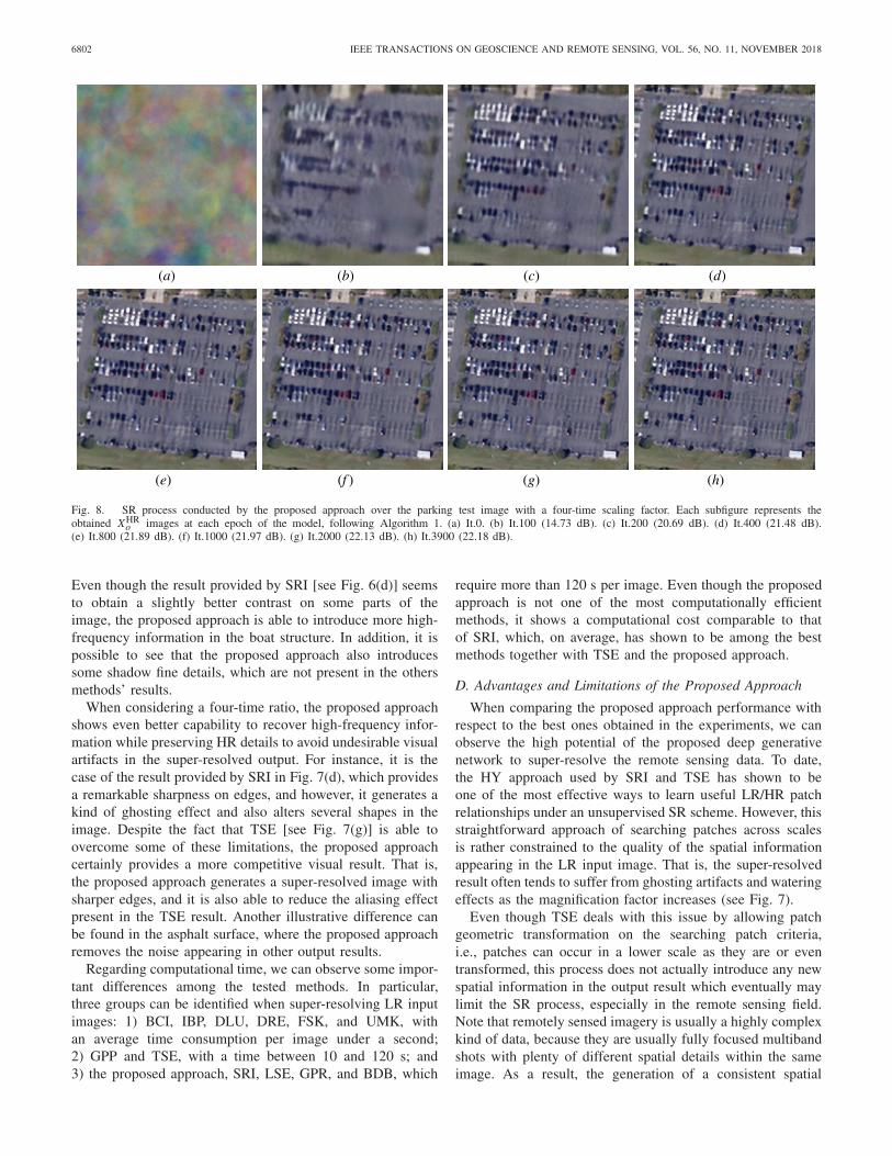
Fig. 8. SR process conducted by the proposed approach over the parking test image with a four-time scaling factor. Each subfigure represents theobtained XHR

o images at each epoch of the model, following Algorithm 1. (a) It.0. (b) It.100 (14.73 dB). (c) It.200 (20.69 dB). (d) It.400 (21.48 dB).(e) It.800 (21.89 dB). (f) It.1000 (21.97 dB). (g) It.2000 (22.13 dB). (h) It.3900 (22.18 dB).

Even though the result provided by SRI [see Fig. 6(d)] seemsto obtain a slightly better contrast on some parts of theimage, the proposed approach is able to introduce more high-frequency information in the boat structure. In addition, it ispossible to see that the proposed approach also introducessome shadow fine details, which are not present in the othersmethods’ results.

When considering a four-time ratio, the proposed approachshows even better capability to recover high-frequency infor-mation while preserving HR details to avoid undesirable visualartifacts in the super-resolved output. For instance, it is thecase of the result provided by SRI in Fig. 7(d), which providesa remarkable sharpness on edges, and however, it generates akind of ghosting effect and also alters several shapes in theimage. Despite the fact that TSE [see Fig. 7(g)] is able toovercome some of these limitations, the proposed approachcertainly provides a more competitive visual result. That is,the proposed approach generates a super-resolved image withsharper edges, and it is also able to reduce the aliasing effectpresent in the TSE result. Another illustrative difference canbe found in the asphalt surface, where the proposed approachremoves the noise appearing in other output results.

Regarding computational time, we can observe some impor-tant differences among the tested methods. In particular,three groups can be identified when super-resolving LR inputimages: 1) BCI, IBP, DLU, DRE, FSK, and UMK, withan average time consumption per image under a second;2) GPP and TSE, with a time between 10 and 120 s; and3) the proposed approach, SRI, LSE, GPR, and BDB, which

require more than 120 s per image. Even though the proposedapproach is not one of the most computationally efficientmethods, it shows a computational cost comparable to thatof SRI, which, on average, has shown to be among the bestmethods together with TSE and the proposed approach.

D. Advantages and Limitations of the Proposed Approach

When comparing the proposed approach performance withrespect to the best ones obtained in the experiments, we canobserve the high potential of the proposed deep generativenetwork to super-resolve the remote sensing data. To date,the HY approach used by SRI and TSE has shown to beone of the most effective ways to learn useful LR/HR patchrelationships under an unsupervised SR scheme. However, thisstraightforward approach of searching patches across scalesis rather constrained to the quality of the spatial informationappearing in the LR input image. That is, the super-resolvedresult often tends to suffer from ghosting artifacts and wateringeffects as the magnification factor increases (see Fig. 7).

Even though TSE deals with this issue by allowing patchgeometric transformation on the searching patch criteria,i.e., patches can occur in a lower scale as they are or eventransformed, this process does not actually introduce any newspatial information in the output result which eventually maylimit the SR process, especially in the remote sensing field.Note that remotely sensed imagery is usually a highly complexkind of data, because they are usually fully focused multibandshots with plenty of different spatial details within the sameimage. As a result, the generation of a consistent spatial


TABLE V

SR RESULTS FOR TEST IMAGES FROM 1 TO 4. THE BEST RESULT FOR EACH IMAGE, SCALING RATIO, AND METRIC IS HIGHLIGHTED IN BOLD FONT

variability becomes a key factor to improve the unsupervisedremote sensing SR process.

Precisely, this is the objective of the proposed approach.In particular, the presented deep generative network learnsthe relationships between the LR and HR domains throughoutseveral convolutional and downsampling layers starting fromthe LR input image. However, this process is affected by

random noise, which is also restricted by the cost function,that is (5), to guarantee a global reconstruction constraint overthe LR input image. That is, the random noise generates newspatial variations as possible solutions to relieve the ill-posednature of the SR problem, while the cost optimizer controlsthat only these variations consistent with respect to the inputLR image are promoted though the network to generate the


TABLE VI


final SR result. Fig. 8 shows the SR process conducted bythe proposed network over the parking test image consideringa four-time scaling factor. As we can see, the reconstructedsuper-resolved result is initially noise; however, the spatialstructures are recovered from a coarser to finer level of detailsas the network iterates.

In a sense, the proposed approach is able to recover aricher variety of high-frequency patterns for a given LR imagedue to its generative nature. In other words, the proposeddeep generative network provides a more flexible unsupervised

SR scheme than the current HY techniques, because it is ableto introduce some spatial variations that are impossible toretrieve from the LR input image. In fact, it is possible tobetter appreciate the proposed approach effectiveness whenonly considering the PSNR metric, which is the most widelyused quality index in SR. Figs. 9 and 10 show the PSNRgain obtained by the three best methods, i.e., the proposedapproach, TSE, and SRI, with respect to the BCI baseline.As we can appreciate, the proposed approach provides someremarkable PSNR improvements in two times; however,


TABLE VII


the PSNR gain is consistently higher when considering a four-time ratio. Note that, with this scaling factor, the level ofuncertainty significantly increases, and it is then when thegenerative process of the proposed approach becomes moreeffective by introducing a higher variety of spatial details.

Although the results obtained by the proposed approachare encouraging, there are two points which deserve to be

mentioned when comparing the proposed approach perfor-mance to the one obtained by the most effective unsuper-vised SR methods: the performance on some metrics and thecomputational cost.

On the one hand, the proposed approach performances onsome metrics, specifically Q-index, SSIM, and SAM, seem notto be superior to the corresponding TSE results. For instance,


Fig. 9. PSNR (dB) results when considering a two-time scaling factor.

Fig. 10. PSNR (dB) results when considering a four-time scaling factor.

Table VII shows that the TSE obtains the best SSIM resultfor the four-time road image (0.8290), whereas the proposedapproach achieves the second best SSIM value (0.8247).However, the proposed approach provides the best PSNRresult (25.69 dB), which is substantially higher than the TSEone (23.86 dB). In spite of the small SSIM differences,it is possible to see the proposed approach advantages whenconsidering the qualitative results. That is, Fig. 10 certainlyshows that TSE magnifies the aliasing effect in the first lineof pedestrian crossing and also generates a kind of wateringeffect on surfaces, whereas the proposed approach is able toobtain a more natural as well as reliable result, even thoughsome image materials seem less contrasted. For the proposedapproach, we adopt a cost function based on the mse in theway many other DL-based SR methods do in the supervisedscheme (see [35], [69], [70]). Logically, our model has adifferent nature because of its unsupervised scheme; however,it seems reasonable to make this consideration, because thePSNR index, which is based on the mse, is one the mostcommonly used metric in SR. Somehow, this definition of thecost function may constrain the performance on some metrics,because the network optimizer works for minimizing the mseand other kinds of metric features are not taken into accountin this optimization process, which eventually may led to asuper-resolved solution with an excellent PSNR performancebut with some small divergences in other figures of merit.

On the other hand, the computational cost of the pro-posed approach may also become a limitation in some spe-cific scenarios. According to the quantitative results shownin Table IV, the proposed approach takes over 300 and 150 s toprocess each input image considering a two-time and four-timeratios, respectively. Even though the proposed approach has

Fig. 11. PSNR evolution for harbor, circular-farmland, industry, and roadtest images considering a four-time scaling ratio versus iteration.

Fig. 12. PSNR evolution for harbor, circular-farmland, industry, and roadtest images considering a four-time scaling ratio versus time.

not shown to be one of the most computationally efficientmethods, three important considerations have to be done tothis extent. First, the computational burden is not only adrawback of the proposed approach but also of any DLarchitecture, because this kind of technology usually providesa more powerful framework to cope with new challengesand tasks. Second, the implementation of our model has notbeen optimized to really exploit the GPU hardware resourcesin order to substantially reduce the resulting computationaltime. That is, we make use of standard functions but furtherefforts could be addressed to generate a much more optimizedversion of the code. Third, we use a general configuration of4000 iterations as a security margin to guarantee a goodnetwork convergence; however, this value could be reducedin order to significantly improve the proposed approach com-putational efficiency. Fig. 11 shows the evolution of thePSNR metric with respect to the number of iterations forharbor, circular-farmland, industry, and road test images witha four-time ratio. As it is possible to see, the network isable to achieve a PSNR result that is very close to theoptimal value after 2000 iterations, and therefore, it wouldbe possible to reduce the number of iterations in order tosignificantly decrease the proposed approach computationaltime. In Fig. 12, we also show the PSNR evolution over time tohighlight the fact that the proposed approach is able to rapidlyconverge to the optimal PSNR value. It should be noted thatwe use a unique network settings in this paper, and therefore,4000 iterations are used to guarantee a good general parameterconvergence, that is, without adapting the network to eachinput image.


V. CONCLUSION AND FUTURE LINES

In this paper, we have presented a new convolutionalgenerator model to super-resolve the LR remote sensing datafrom an unsupervised perspective. Specifically, the proposedapproach is initially able to learn relationships between theLR and HR domains while generating consistent random spa-tial variations. Then, the data are symmetrically projected tothe target resolution, guaranteeing a reconstruction constraintover the LR input image. Our experiments, conducted usingseveral test images, two scaling factors, and 12 different SRmethods available in the literature, reveal the competitiveperformance of the proposed approach when super-resolvingremotely sensed images.

One of the main conclusions that arises from this paperis the potential of deep generative models to cope with theunsupervised SR problem because of their capabilities tointroduce new spatial details not present in the input LRimage. As opposed to the common (HY) SR trend, whichonly relies on the patch relationships learned across scales,the proposed approach extends this scheme by introducingsome spatial variations that allow the network to retrieve newspatial patterns that are consistent with the input LR image.

According to the conducted experiments, the proposedapproach obtains a competitive global performance over theconsidered remote sensing test images in terms of both quan-titative and qualitative SR results. Regarding the NRMSE,PSNR, and ERGAS metrics, the SR framework proposed inthis paper obtains, on average, the best performance. Whenconsidering Q-index, SSIM, and SAM, TSE tends to providethe best average result, but the proposed approach is stillable to perform among the best methods, especially whenconsidering a four-time scaling factor.

Although the proposed approach results are encouraging asa generative SR model in remote sensing, the method still hassome limitations, which provide room for improvement byconducting additional research on unsupervised SR. Specifi-cally, our future work will be aimed at the following directions:1) extending the cost function to simultaneously take intoaccount several image quality metrics and also to extend itwith the aim of implementing a noise reduction scheme fora different kind of input data; 2) adapting the convolutionalkernel size to each specific input image; and 3) reducingthe model computational cost by designing new strategies toactively control the number of iterations depending on theinput image.

ACKNOWLEDGMENT

The authors would like to thank the editors and reviewersfor their outstanding comments and suggestions, which greatlyhelped us to improve the technical quality and presentation ofthis paper.

REFERENCES

[1] J. A. Benediktsson, J. Chanussot, and W. M. Moon, “Very high-resolution remote sensing: Challenges and opportunities [point of view],”Proc. IEEE, vol. 100, no. 6, pp. 1907–1910, Jun. 2012.

[2] M.-T. Pham, E. Aptoula, and S. Lefèvre, “Feature profiles from attributefiltering for classification of remote sensing images,” IEEE J. Sel.Topics Appl. Earth Observ. Remote Sens., vol. 11, no. 1, pp. 249–256,Jan. 2018.

[3] A. E. Maxwell, T. A. Warner, and F. Fang, “Implementation of machine-learning classification in remote sensing: An applied review,” Int. J.Remote Sens., vol. 39, no. 9, pp. 2784–2817, 2018.

[4] G. Sumbul, R. G. Cinbis, and S. Aksoy, “Fine-grained object recognitionand zero-shot learning in remote sensing imagery,” IEEE Trans. Geosci.Remote Sens., vol. 56, no. 2, pp. 770–779, Feb. 2018.

[5] X. Kang, Y. Huang, S. Li, H. Lin, and J. A. Benediktsson, “Extendedrandom walker for shadow detection in very high resolution remotesensing images,” IEEE Trans. Geosci. Remote Sens., vol. 56, no. 2,pp. 867–876, Feb. 2018.

[6] H. Lin, Z. Shi, and Z. Zou, “Fully convolutional network with taskpartitioning for inshore ship detection in optical remote sensing images,”IEEE Geosci. Remote Sens. Lett., vol. 14, no. 10, pp. 1665–1669,Oct. 2017.

[7] T. Wu, J. Luo, J. Fang, J. Ma, and X. Song, “Unsupervised object-based change detection via a Weibull mixture model-based binarizationfor high-resolution remote sensing images,” IEEE Geosci. Remote Sens.Lett., vol. 15, no. 1, pp. 63–67, Jan. 2018.

[8] Z. Liu, G. Li, G. Mercier, Y. He, and Q. Pan, “Change detection inheterogenous remote sensing images via homogeneous pixel transfor-mation,” IEEE Trans. Image Process., vol. 27, no. 4, pp. 1822–1834,Apr. 2018.

[9] A. S. Belward and J. O. Skøien, “Who launched what, when and why;trends in global land-cover observation capacity from civilian earthobservation satellites,” ISPRS J. Photogramm. Remote Sens., vol. 103,pp. 115–128, May 2015.

[10] J. R. Jensen and K. Lulla, “Introductory digital image processing: Aremote sensing perspective,” Geocarto Int., vol. 2, no. 1, p. 65, 2008,doi: 10.1080/10106048709354084.

[11] S. C. Park, M. K. Park, and M. G. Kang, “Super-resolution imagereconstruction: A technical overview,” IEEE Signal Process. Mag.,vol. 20, no. 3, pp. 21–36, May 2003.

[12] P. Milanfar, Super-Resolution Imaging. Boca Raton, FL, USA:CRC Press, 2010.

[13] L. Yue, H. Shen, J. Li, Q. Yuanc, H. Zhang, and L. Zhang, “Image super-resolution: The techniques, applications, and future,” Signal Process.,vol. 128, pp. 389–408, Nov. 2016.

[14] A. Garzelli, “A review of image fusion algorithms based on the super-resolution paradigm,” Remote Sens., vol. 8, no. 10, p. 797, Sep. 2016.

[15] C.-Y. Yang, C. Ma, and M.-H. Yang, “Single-image super-resolution:A benchmark,” in Proc. Eur. Conf. Comput. Vis., 2014, pp. 372–386.

[16] A. Punnappurath, T. M. Nimisha, and A. N. Rajagopalan, “Multi-imageblind super-resolution of 3D scenes,” IEEE Trans. Image Process.,vol. 26, no. 11, pp. 5337–5352, Nov. 2017.

[17] D. Yang, Z. Li, Y. Xia, and Z. Chen, “Remote sensing image super-resolution: Challenges and approaches,” in Proc. IEEE Int. Conf. Digit.Signal Process. (DSP), Jul. 2015, pp. 196–200.

[18] L. Alparone, B. Aiazzi, S. Baronti, and A. Garzelli, Remote SensingImage Fusion. Boca Raton, FL, USA: CRC Press, 2015.

[19] C. M. Bishop, Neural Networks for Pattern Recognition. Oxford,U.K.: Clarendon, 1995. [Online]. Available: https://books.google.es/books?id=-aAwQO_-rXwC

[20] J. A. Benediktsson, P. H. Swain, and O. K. Ersoy, “Conjugate-gradient neural networks in classification of multisource and very-high-dimensional remote sensing data,” Int. J. Remote Sens., vol. 14, no. 15,pp. 2883–2903, 1993. [Online]. Available: http://www.tandfonline.com/doi/abs/10.1080/01431169308904316

[21] P. M. Atkinson and A. R. L. Tatnall, “Introduction neural networks inremote sensing,” Int. J. Remote Sens., vol. 18, no. 4, pp. 699–709, 1997,doi: 10.1080/014311697218700.

[22] H. Yang, “A back-propagation neural network for mineralogical mappingfrom AVIRIS data,” Int. J. Remote Sens., vol. 20, no. 1, pp. 97–110,1999, doi: 10.1080/014311699213622.

[23] Y. LeCun, Y. Bengio, and G. Hinton, “Deep learning,” Nature, vol. 521,pp. 436–444, May 2015.

[24] I. Goodfellow, Y. Bengio, and A. Courville, Deep Learning. Cambridge,MA, USA: MIT Press, 2016.

[25] Y. Bengio, “Learning deep architectures for AI,” Found. Trends Mach.Learn., vol. 2, no. 1, pp. 1–127, 2009.

[26] M. Sharma, S. Chaudhury, and B. Lall, “Deep learning based frame-works for image super-resolution and noise-resilient super-resolution,”in Proc. Int. Joint Conf. Neural Netw. (IJCNN), May 2017, pp. 744–751.

[27] K. Makantasis, K. Karantzalos, A. Doulamis, and N. Doulamis, “Deepsupervised learning for hyperspectral data classification through con-volutional neural networks,” in Proc. IEEE Int. Geosci. Remote Sens.Symp. (IGARSS), Jul. 2015, pp. 4959–4962.

http://dx.doi.org/10.1080/10106048709354084

http://dx.doi.org/10.1080/014311697218700

http://dx.doi.org/10.1080/014311699213622


[28] M. Castelluccio, G. Poggi, C. Sansone, and L. Verdoliva, “Land use clas-sification in remote sensing images by convolutional neural networks,”CoRR, 2015. [Online]. Available: http://arxiv.org/abs/1508.00092

[29] Y. Chen, H. Jiang, C. Li, X. Jia, and P. Ghamisi, “Deep feature extrac-tion and classification of hyperspectral images based on convolutionalneural networks,” IEEE Trans. Geosci. Remote Sens., vol. 54, no. 10,pp. 6232–6251, Oct. 2016. [Online]. Available: http://ieeexplore.ieee.org/document/7514991/

[30] M. E. Paoletti, J. M. Haut, J. Plaza, and A. Plaza, “A new deepconvolutional neural network for fast hyperspectral image classification,”ISPRS J. Photogramm. Remote Sens., to be published.

[31] Q. Yuan, Y. Wei, X. Meng, H. Shen, and L. Zhang, “A multiscale andmultidepth convolutional neural network for remote sensing imagerypan-sharpening,” IEEE J. Sel. Topics Appl. Earth Observ. Remote Sens.,vol. 11, no. 3, pp. 978–989, Mar. 2018.

[32] R. Dian, S. Li, A. Guo, and L. Fang, “Deep hyperspectral imagesharpening,” IEEE Trans. Neural Netw. Learn. Syst., to be published.

[33] Q. Zhang, Q. Yuan, C. Zeng, X. Li, and Y. Wei, “Missing datareconstruction in remote sensing image with a unified spatial-temporal-spectral deep convolutional neural network,” IEEE Trans. Geosci.Remote Sens., to be published.

[34] L. Liebel and M. Körner, “Single-image super resolution for multispec-tral remote sensing data using convolutional neural networks,” ISPRS-Int. Arch. Photogramm., Remote Sens. Spatial Inf. Sci., vol. XLI-B3,pp. 883–890, Jun. 2016.

[35] C. Dong, C. C. Loy, K. He, and X. Tang, “Image super-resolution usingdeep convolutional networks,” IEEE Trans. Pattern Anal. Mach. Intell.,vol. 38, no. 2, pp. 295–307, Feb. 2016.

[36] T. Y. Han, Y. J. Kim, and B. C. Song, “Convolutional neural network-based infrared image super resolution under low light environment,”in Proc. 25th Eur. Signal Process. Conf. (EUSIPCO), Aug./Sep. 2017,pp. 803–807.

[37] C. Li, Z. Ren, B. Yang, X. Wan, and J. Wang, “Texture-centralized deepconvolutional neural network for single image super resolution,” in Proc.Chin. Autom. Congr. (CAC), Oct. 2017, pp. 3707–3710.

[38] X. Du, Y. He, J. Li, and X. Xie, “Single image super-resolution viamulti-scale fusion convolutional neural network,” in Proc. IEEE 8th Int.Conf. Awareness Sci. Technol. (iCAST), Nov. 2017, pp. 544–551.

[39] O. Fırat and F. T. Y. Vural, “Representation learning with convolutionalsparse autoencoders for remote sensing,” in Proc. 21st Signal Process.Commun. Appl. Conf. (SIU), Apr. 2013, pp. 1–4.

[40] W. Cui, Q. Zhou, and Z. Zheng, “Application of a hybrid model based ona convolutional auto-encoder and convolutional neural network in object-oriented remote sensing classification,” Algorithms, vol. 11, no. 1, p. 9,Jan. 2018. [Online]. Available: http://www.mdpi.com/1999-4893/11/1/9

[41] R. Tanase, M. Datcu, and D. Raducanu, “A convolutional deepbelief network for polarimetric SAR data feature extraction,” inProc. IEEE Int. Geosci. Remote Sens. Symp. (IGARSS), Jul. 2016,pp. 7545–7548.

[42] D. Lin, K. Fu, Y. Wang, G. Xu, and X. Sun, “MARTA GANs: Unsuper-vised representation learning for remote sensing image classification,”IEEE Geosci. Remote Sens. Lett., vol. 14, no. 11, pp. 2092–2096,Nov. 2017.

[43] Z. Zuo et al., “Convolutional recurrent neural networks: Learning spatialdependencies for image representation,” in Proc. IEEE Conf. Comput.Vis. Pattern Recognit. Workshops (CVPRW), Jun. 2015, pp. 18–26.

[44] J. Long, E. Shelhamer, and T. Darrell, “Fully convolutional networksfor semantic segmentation,” in Proc. IEEE Conf. Comput. Vis. PatternRecognit. Workshops (CVPRW), Jun. 2015, pp. 3431–3440.

[45] A. Newell, K. Yang, and J. Deng, “Stacked hourglass networks forhuman pose estimation,” in Proc. Eur. Conf. Comput. Vis. Cham,Switzerland: Springer, Oct. 2016, pp. 483–499.

[46] I. Melekhov, J. Ylioinas, J. Kannala, and E. Rahtu, “Image-basedlocalization using hourglass networks,” CoRR, 2017. [Online]. Available:http://arxiv.org/abs/1703.07971

[47] M. E. Paoletti, J. M. Haut, J. Plaza, and A. Plaza, “Yinyang K-meansclustering for hyperspectral image analysis,” in Proc. 17th Int. Conf.Comput. Math. Methods Sci. Eng., 2017, pp. 1625–1636.

[48] C. González, S. Sánchez, A. Paz, J. Resano, D. Mozos, and A. Plaza,“Use of FPGA or GPU-based architectures for remotely sensed hyper-spectral image processing,” Integr., VLSI J., vol. 46, no. 2, pp. 89–103,Mar. 2013.

[49] A. Plaza, J. Plaza, A. Paz, and S. Sánchez, “Parallel hyperspectral imageand signal processing [applications corner],” IEEE Signal Process. Mag.,vol. 28, no. 3, pp. 119–126, May 2011.

[50] J. M. Haut, M. Paoletti, J. Plaza, and A. Plaza, “Cloud implementationof the K-means algorithm for hyperspectral image analysis,” J. Super-comput., vol. 73, no. 1, pp. 514–529, Jan. 2017.

[51] J. M. Haut, M. E. Paoletti, A. Paz-Gallardo, J. Plaza, and A. Plaza,“Cloud implementation of logistic regression for hyperspectral imageclassification,” in Proc. 17th Int. Conf. Comput. Math. Methods Sci.Eng. (CMMSE), 2017, pp. 1063–2321.

[52] A. J. Plaza, C.-I. Chang, L. Di, and Y. Bai, High Performance Com-puting in Remote Sensing (Computer & Information Science Series).Boca Raton, FL, USA: Chapman & Hall, 2008.

[53] K. Nasrollahi and T. B. Moeslund, “Super-resolution: A comprehensivesurvey,” Mach. Vis. Appl., vol. 25, no. 6, pp. 1423–1468, 2014.

[54] R. Fernandez-Beltran, P. Latorre-Carmona, and F. Pla, “Single-framesuper-resolution in remote sensing: A practical overview,” Int. J. RemoteSens., vol. 38, no. 1, pp. 314–354, 2017.

[55] M. Irani and S. Peleg, “Improving resolution by image registration,”CVGIP, Graph. Models Image Process., vol. 53, no. 3, pp. 231–239,May 1991.

[56] J. Sun, Z. Xu, and H.-Y. Shum, “Image super-resolution using gradientprofile prior,” in Proc. IEEE Conf. Comput. Vis. Pattern Recognit.,Jun. 2008, pp. 1–8.

[57] L. B. Lucy, “An iterative technique for the rectification of observeddistributions,” Astron. J., vol. 79, no. 6, p. 745, 1974.

[58] R. C. Gonzalez and R. E. Woods, Digital Image Processing, 3rd ed.Englewood Cliffs, NJ, USA: Prentice-Hall, 2006.

[59] G. Deng, “A generalized unsharp masking algorithm,” IEEE Trans.Image Process., vol. 20, no. 5, pp. 1249–1261, May 2011.

[60] J. Yang, J. Wright, T. S. Huang, and Y. Ma, “Image super-resolutionvia sparse representation,” IEEE Trans. Image Process., vol. 19, no. 11,pp. 2861–2873, Nov. 2010.

[61] R. Timofte, V. De Smet, and L. Van Gool, “Anchored neighborhoodregression for fast example-based super-resolution,” in Proc. IEEE Int.Conf. Comput. Vis., Dec. 2013, pp. 1920–1927.

[62] C. Dong et al., “Learning a deep convolutional network for image super-resolution,” in Computer Vision—ECCV, vol. 8692, D. Fleet, Ed. Cham,Switzerland: Springer, 2014, pp. 184–199.

[63] G. Polatkan, M. Zhou, L. Carin, D. Blei, and I. Daubechies, “A Bayesiannonparametric approach to image super-resolution,” IEEE Trans. PatternAnal. Mach. Intell., vol. 37, no. 2, pp. 346–358, Feb. 2015.

[64] D. Glasner, S. Bagon, and M. Irani, “Super-resolution from a sin-gle image,” in Proc. IEEE Int. Conf. Comput. Vis., Sep./Oct. 2009,pp. 349–356.

[65] J.-B. Huang, A. Singh, and N. Ahuja, “Single image super-resolutionfrom transformed self-exemplars,” in Proc. IEEE Conf. Comput. Vis.Pattern Recognit., Jun. 2015, pp. 5197–5206.

[66] T. Michaeli and M. Irani, “Blind deblurring using internal patch recur-rence,” in Proc. Eur. Conf. Comput. Vis., 2014, pp. 783–798.

[67] S. Baker and T. Kanade, “Limits on super-resolution and how tobreak them,” IEEE Trans. Pattern Anal. Mach. Intell., vol. 24, no. 9,pp. 1167–1183, Sep. 2002.

[68] V. Syrris, S. Ferri, D. Ehrlich, and M. Pesaresi, “Image enhancement andfeature extraction based on low-resolution satellite data,” IEEE J. Sel.Topics Appl. Earth Observ. Remote Sens., vol. 8, no. 5, pp. 1986–1995,May 2015.

[69] J. Kim, J. K. Lee, and K. M. Lee, “Accurate image super-resolutionusing very deep convolutional networks,” in Proc. IEEE Conf. Comput.Vis. Pattern Recognit., Jun. 2016, pp. 1646–1654.

[70] B. Lim, S. Son, H. Kim, S. Nah, and K. M. Lee, “Enhanced deepresidual networks for single image super-resolution,” in Proc. IEEEConf. Comput. Vis. Pattern Recognit. (CVPR) Workshops, Jul. 2017,vol. 1, no. 2, p. 3.

[71] F. A. Mianji, Y. Gu, Y. Zhang, and J. Zhang, “Enhanced self-trainingsuperresolution mapping technique for hyperspectral imagery,” IEEEGeosci. Remote Sens. Lett., vol. 8, no. 4, pp. 671–675, Jul. 2011.

[72] J. M. Bioucas-Dias et al., “Hyperspectral unmixing overview: Geomet-rical, statistical, and sparse regression-based approaches,” IEEE J. Sel.Topics Appl. Earth Observ. Remote Sens., vol. 5, no. 2, pp. 354–379,Apr. 2012.

[73] W. Hu, Y. Huang, L. Wei, F. Zhang, and H. Li, “Deep con-volutional neural networks for hyperspectral image classification,”J. Sensors, vol. 2015, 2015, Art. no. 258619. [Online]. Available:https://doi.org/10.1155/2015/258619

[74] M. E. Paoletti, J. M. Haut, J. Plaza, A. Plaza, Q. Liu, and R. Hang,“Multicore implementation of the multi-scale adaptive deep pyramidmatching model for remotely sensed image classification,” in Proc.IEEE Int. Geosci. Remote Sens. Symp. (IGARSS), Fort Worth, TX, USA,Dec. 2017, pp. 2247–2250.


[75] S. Yu, S. Jia, and C. Xu, “Convolutional neural networksfor hyperspectral image classification,” Neurocomputing, vol. 219,pp. 88–98, Jan. 2017. [Online]. Available: http://linkinghub.elsevier.com/retrieve/pii/S0925231216310104

[76] V. Nair and G. E. Hinton, “Rectified linear units improve restrictedBoltzmann machines,” in Proc. 27th Int. Conf. Mach. Learn. (ICML),J. Fürnkranz and T. Joachims, Eds. Madison, WI, USA: Omnipress,2010, pp. 807–814.

[77] B. Xu, N. Wang, T. Chen, and M. Li. (2015). “Empirical evaluationof rectified activations in convolutional network.” [Online]. Available:https://arxiv.org/abs/1505.00853

[78] A. L. Maas, A. Y. Hannun, and A. Y. Ng, “Rectifier nonlinearitiesimprove neural network acoustic models,” in Proc. Int. Conf. Mach.Learn. (ICML), 2013, p. 30.

[79] D. P. Kingma and J. L. Ba, “Adam: A method for stochastic optimiza-tion,” in Proc. Int. Conf. Learn. Represent. (ICLR), 2015.

[80] K. Turkowski, “Filters for common resampling tasks,” in GraphicsGems, A. S. Glassner, Ed. San Francisco, CA, USA: Academic, 1990,pp. 147–165.

[81] D. P. Kingma and J. L. Ba, “Adam: A method for stochastic optimiza-tion,” CoRR, 2014. [Online]. Available: http://arxiv.org/abs/1412.6980

[82] Q. Huynh-Thu and M. Ghanbari, “Scope of validity of PSNR inimage/video quality assessment,” Electron. Lett., vol. 44, no. 13,pp. 800–801, Jun. 2008.

[83] R. H. Yuhas, A. F. Goetz, and J. W. Boardman, “Discriminationamong semi-arid landscape endmembers using the Spectral AngleMapper (SAM) algorithm,” Tech. Rep., 1992. [Online]. Available:https://ntrs.nasa.gov/search.jsp?R=19940012238

[84] Z. Wang, A. C. Bovik, H. R. Sheikh, and E. P. Simoncelli, “Imagequality assessment: From error visibility to structural similarity,” IEEETrans. Image Process., vol. 13, no. 4, pp. 600–612, Apr. 2004.

[85] M. A. Veganzones, M. Simões, G. Licciardi, N. Yokoya,J. M. Bioucas-Dias, and J. Chanussot, “Hyperspectral super-resolutionof locally low rank images from complementary multisource data,”IEEE Trans. Image Process., vol. 25, no. 1, pp. 274–288, Jan. 2016.

[86] A. Paszke et al., “Automatic differentiation in PyTorch,” inProc. NIPS-W, 2017.

[87] C. Ledig et al., “Photo-realistic single image super-resolution usinga generative adversarial network,” in Proc. IEEE Conf. Comput. Vis.Pattern Recognit. (CVPR), Jul. 2017, pp. 105–114.

[88] Y. Yang and S. Newsam, “Bag-of-visual-words and spatial extensionsfor land-use classification,” in Proc. 18th SIGSPATIAL Int. Conf.Advances Geograph. Inf. Syst. (GIS). New York, NY, USA: ACM, 2010,pp. 270–279. [Online]. Available: http://doi.acm.org/10.1145/1869790.1869829

[89] Q. Zou, L. Ni, T. Zhang, and Q. Wang, “Deep learning based featureselection for remote sensing scene classification,” IEEE Geosci. RemoteSens. Lett., vol. 12, no. 11, pp. 2321–2325, Nov. 2015.

[90] G. Cheng, J. Han, and X. Lu, “Remote sensing image scene classifi-cation: Benchmark and state of the art,” Proc. IEEE, vol. 105, no. 10,pp. 1865–1883, Oct. 2017.

[91] K. Turkowski, “Filters for common resampling tasks,” in GraphicsGems. San Francisco, CA, USA: Academic, 1990, pp. 147–165.

[92] G. Freedman and R. Fattal, “Image and video upscaling from local self-examples,” ACM Trans. Graph., vol. 30, no. 2, pp. 1–11, Apr. 2011.

[93] H. He and W.-C. Siu, “Single image super-resolution using Gaussianprocess regression,” in Proc. IEEE Conf. Comput. Vis. Pattern Recognit.,Jun. 2011, pp. 449–456.

[94] N. Zhao, Q. Wei, A. Basarab, N. Dobigeon, D. Kouamé, andJ.-Y. Tourneret, “Fast single image super-resolution using a new analyt-ical solution for 2–2 problems,” IEEE Trans. Image Process., vol. 25,no. 8, pp. 3683–3697, Aug. 2016.

Juan Mario Haut (S’17) received the B.Sc.and M.Sc. degrees in computer engineering fromthe University of Extremadura, Cáceres, Spain,in 2011 and 2014, respectively, where he is currentlypursuing the Ph.D. degree with a University TeacherTraining Program from the Spanish Ministry ofEducation.

He is also a member of the Hyperspectral Com-puting Laboratory, Department of Computers andCommunications, University of Extremadura. Hisresearch interests include remote sensing and analy-

sis of very high spectral resolution with the current focus on deep learningand cloud computing. https://mhaut.github.io/.

Ruben Fernandez-Beltran received the B.Sc.degree in computer science, the M.Sc. degree inintelligent systems, and the Ph.D. degree in com-puter science from Universitat Jaume I, Castellónde la Plana, Spain, in 2007, 2011, and 2016,respectively.

He has been a Visiting Scientist with the Uni-versity of Bristol, Bristol, U.K. Since 2017, hehas been a Visiting Post-Doctoral Researcher withthe Hyperspectral Computing Laboratory, Universityof Extremadura, Cáceres, Spain. He is currently a

Post-Doctoral Researcher with the Computer Vision Group, University JaumeI, as a member of the Institute of New Imaging Technologies. His researchinterests include multimedia retrieval, spatio–spectral image analysis, patternrecognition techniques applied to image processing, and remote sensing.

Dr. Fernandez-Beltran is a member of the Spanish Association for PatternRecognition and Image Analysis, which is part of the International Associationfor Pattern Recognition. He received the Outstanding Ph.D. DissertationAward at Universitat Jaume I in 2017.

Mercedes E. Paoletti (S’17) received the B.Sc.and M.Sc. degrees in computer engineering fromthe University of Extremadura, Cáceres, Spain,in 2014 and 2016, respectively, where she is cur-rently pursuing the Ph.D. degree with a UniversityTeacher Training Program from the Spanish Ministryof Education.

She is also a member of the HyperspectralComputing Laboratory, Department of Technologyof Computers and Communications, University ofExtremadura. Her research interests include remote

sensing and analysis of very high spectral resolution with the current focuson deep learning and high performance computing.

Javier Plaza (M’09–SM’15) received the M.Sc.and Ph.D. degrees from the Hyperspectral Com-puting Laboratory, Department of Technology ofComputers and Communications, University ofExtremadura, Cáceres, Spain, in 2004 and 2008,respectively.

He is currently a member of the HyperspectralComputing Laboratory, Department of Technologyof Computers and Communications, University ofExtremadura. He has authored more than 150 publi-cations, including over 50 Journal Citations Reports

journal papers, ten book chapters, and 90 peer-reviewed conference proceedingpapers. His research interests include hyperspectral data processing andparallel computing of remote sensing data.

Dr. Plaza was a recipient of the Outstanding Ph.D. Dissertation Awardat the University of Extremadura in 2008 and the Best Column Award ofthe IEEE Signal Processing Magazine in 2015 and the most highly citedpaper (2005–2010) in the Journal of Parallel and Distributed Computing.He received the best paper awards at the IEEE International Conferenceon Space Technology and the IEEE Symposium on Signal Processing andInformation Technology. He has guest edited four special issues on hyper-spectral remote sensing for different journals. He is an Associate Editor of theIEEE GEOSCIENCE AND REMOTE SENSING LETTERS and the IEEE RemoteSensing Code Library. http://www.umbc.edu/rssipl/people/jplaza.


Antonio Plaza (M’05–SM’07–F’15) received theM.Sc. and Ph.D. degrees in computer engineer-ing from the Hyperspectral Computing Laboratory,Department of Technology of Computers and Com-munications, University of Extremadura, Cáceres,Spain, in 1999 and 2002, respectively.

He is currently the Head of the HyperspectralComputing Laboratory, Department of Technologyof Computers and Communications, University ofExtremadura. He has authored more than 600 publi-cations, including over 200 Journal Citations Reports

journal papers (over 160 in IEEE journals), 23 book chapters, and around300 peer-reviewed conference proceeding papers. His research interestsinclude hyperspectral data processing and parallel computing of remotesensing data.

Dr. Plaza is a fellow of the IEEE for his contributions to hyperspec-tral data processing and parallel computing of Earth observation data.He was also a member of the Steering Committee of the IEEE JOURNAL

OF SELECTED TOPICS IN APPLIED EARTH OBSERVATIONS AND REMOTE

SENSING (JSTARS). He was a recipient of the Best Column Award of theIEEE Signal Processing Magazine in 2015 and the 2013 Best Paper Awardof the JSTARS journal and the most highly cited paper (2005–2010) inthe Journal of Parallel and Distributed Computing. He received the bestpaper awards at the IEEE International Conference on Space Technologyand the IEEE Symposium on Signal Processing and Information Technology.He served as the Director of Education Activities for the IEEE Geoscience andRemote Sensing Society (GRSS) from 2011 to 2012 and the President of theSpanish Chapter of the IEEE GRSS from 2012 to 2016. He was a recipient ofthe recognition of Best Reviewers of the IEEE GEOSCIENCE AND REMOTE

SENSING LETTERS in 2009 and the recognition of Best Reviewers of theIEEE TRANSACTIONS ON GEOSCIENCE AND REMOTE SENSING in 2010,for which he served as an Associate Editor from 2007 to 2012. He is alsoan Associate Editor of the IEEE ACCESS (receiving a recognition as anoutstanding Associate Editor of the journal in 2017) and was a memberof the Editorial Board of the IEEE GEOSCIENCE AND REMOTE SENSINGNEWSLETTER from 2011 to 2012 and the IEEE Geoscience and RemoteSensing Magazine in 2013. He has reviewed more than 500 manuscriptsfor over 50 different journals. He has guest edited ten special issues onhyperspectral remote sensing for different journals. He served as an Editor-in-Chief of the IEEE TRANSACTIONS ON GEOSCIENCE AND REMOTE SENSING

from 2013 to 2017. http://www.umbc.edu/rssipl/people/aplaza.

Filiberto Pla received the B.Sc. and Ph.D. degreesin physics from the Universitat de València, Valen-cia, Spain, in 1989 and 1993, respectively.

He has been a Visiting Scientist with the SilsoeResearch Institute, Bedford, U.K., the University ofSurrey, Guildford, U.K., the University of Bristol,Bristol, U.K., the Institut national de recherche ensciences et technologies pour l’environnement etl’agriculture, Montpellier, France, the University ofGenoa, Genoa, Italy, the Instituto Superior Tcnico ofLisbon, Lisbon, Portugal, the Swiss Federal Institute

of Technology–ETH Zürich, Zürich, Switzerland, the Idiap Research Institute,Martigny, Switzerland, the Technical University of Delft, Delft, The Nether-lands, and Mid Sweden University, Sundsvall, Sweden. He has also been theDirector of the Institute of New Imaging Technologies, University Jaume I,Castellón de la Plana, Spain, where he is currently a Full Professor with theDepartament de Llenguatges i Sistemes Informàtics. His research interestsinclude color and spectral image analysis, visual motion analysis, 3-D imagevisualization, and pattern recognition techniques applied to image processing.

Dr. Pla is a member of the Spanish Association for Pattern Recognition andImage Analysis, which is a member of the International Association for PatternRecognition.

a new deep generative network for unsupervised …...6792 ieee transactions on geoscience and remote...

Documents