A New General Continuous-Time State Task Network Formulation for Short-Term Scheduling of Multipurpose Batch Plants

Christos T. Maravelias, Ignacio E. Grossmann∗

Department of Chemical Engineering, Carnegie Mellon University Pittsburgh, PA 15213, USA

November 2002 / Rev. March 2003

Abstract A new continuous time MILP model for the short-term scheduling of multipurpose batch plants is presented. The proposed model relies on the State Task Network (STN) and addresses the general problem of batch scheduling, accounting for resource (utility) constraints, variable batch sizes and processing times, various storage policies (UIS/FIS/NIS/ZW), batch mixing/splitting, and sequence-dependent changeover times. The key features of the proposed model are the following: (a) a continuous time representation is used, common for all units, (b) assignment constraints are expressed using binary variables that are defined only for tasks, not for units, (c) start times of tasks are eliminated; thus, time matching constraints are used only for the finish times of tasks, and (d) a new class of valid inequalities that improves the LP relaxation is added to the MILP formulation. Compared to other general continuous STN formulations, the proposed model is significantly faster. Compared to event-driven formulations, it is more general as it accounts for resources other than equipment and often gives better solutions being equally fast. The application of the model is illustrated through four example problems.

1. Introduction The problem of short-term scheduling of multipurpose batch plants has received considerable attention during the last decade. Kondili et al. (1993) introduced the State Task Network (STN) and proposed a discrete-time MILP model, where the time horizon is divided into time periods of equal duration. Since the resulting models have many binary variables, Shah et al. (1993) developed a reformulation and specific techniques to reduce the computational times for discrete-time STN models. Pantelides (1995) proposed the alternative representation and formulation of the Resource Task Network (RTN); Schilling and Pantelides (1996) developed a continuous-time MILP model, based on the RTN representation, and a novel branch-and-bound algorithm that branches on both continuous and discrete variables. Zhang and Sargent (1996) and Mockus and Reklaitis (1999) proposed MINLP continuous-time representations for

∗ To whom all correspondence should be addressed. Tel: 412-268-3642, Fax: 412-268-7139, E-mail: grossmann@cmu.edu,

2

the scheduling of batch and continuous processes. Ierapetritou and Floudas (1998a) proposed a new MILP formulation based on event points for the scheduling of batch and continuous multipurpose plants. Despite the improved formulations, the specialized algorithms and the recent improvements in computer hardware and optimization software, the short-term scheduling of STN multipurpose batch plants in continuous time remains a difficult problem to solve. In an effort to reduce problem size and computational time, several authors have proposed various approaches during the last two years (Rodriguez et al. 2001; Mendez et al., 2000; Lee et al. 2001; Giannelos and Georgiadis, 2002). In most of these approaches, however, the authors make specific assumptions that on the one hand lead to more compact formulations, but, on the other hand address only specific cases of the general short-term scheduling problem. Some of the most common assumptions that result in significant reductions in problem size are (a) no batch splitting and (b) no resource constraints other than those on equipment units. As will be illustrated later, even weaker assumptions give rise to formulations that cannot account for all the instances that may appear in a multipurpose batch plant. In this work, we propose a new general State Task Network MILP model for the short-term scheduling of multipurpose batch plants in continuous time that accounts for resource constraints other than equipment (utilities), variable batch sizes and processing times, various storage policies (UIS/FIS/NIS/ZW) including shared storage, sequence dependent changeover times and allows for batch mixing/splitting. The paper is structured as follows. In section 2, we briefly discuss the different time representation approaches proposed in the literature and we outline the proposed approach. The problem statement is presented in section 3. The mathematical formulation and its derivation are described in section 4 and some remarks are presented in section 5. Four examples are presented in the last section.

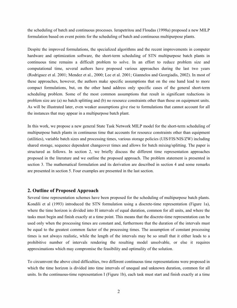
2. Outline of Proposed Approach Several time representation schemes have been proposed for the scheduling of multipurpose batch plants. Kondili et al (1993) introduced the STN formulation using a discrete-time representation (Figure 1a), where the time horizon is divided into H intervals of equal duration, common for all units, and where the tasks must begin and finish exactly at a time point. This means that the discrete-time representation can be used only when the processing times are constant and, furthermore that the duration of the intervals must be equal to the greatest common factor of the processing times. The assumption of constant processing times is not always realistic, while the length of the intervals may be so small that it either leads to a prohibitive number of intervals rendering the resulting model unsolvable, or else it requires approximations which may compromise the feasibility and optimality of the solution. To circumvent the above cited difficulties, two different continuous time representations were proposed in which the time horizon is divided into time intervals of unequal and unknown duration, common for all units. In the continuous-time representation I (Figure 1b), each task must start and finish exactly at a time

3

point (Zhang and Sargent, 1995; Schilling and Pantelides, 1996; Mockus and Reklaitis, 1999), while in the representation II (Figure 1c), each task must start at a time point but it may not finish at a time point (Castro et al., 2001). In both representations, the number of time points is determined with an iterative procedure, during which the number of time points is increased by one until there is no improvement in the objective function. Since time points are not fixed, constraints that match a time point with the start (or finish) of a task are necessary. These constraints are big-M constraints that result in poor LP relaxations. On the other hand, the continuous-time representation accounts for variable processing times, and is more realistic than the discrete representation. It also requires significantly fewer time intervals and, hence, it leads to smaller problems.

U1U2

.

.UN

0 1 2 3 … H-1 H t

(a) Discrete-Time Representation

0 1 2 3 … H-1 H t

(b) Continuous-Time Representation I

0 1 2 3 … H-1 H t

(c) Continuous-Time Representation II

t

k

k

k+1

(d) Event-Point Representation

k

U1U2

.

.UN

U1U2

.

.UN

U1U2

.

.UN

…

…

Figure 1: Alternative time-domain representations.

An alternative approach is the event-point representation (Figure 1d) proposed by Ierapetritou and Floudas (1998a), in which the time intervals are not common for all units. In this approach, the time horizon is divided into a number of events which are different for each unit, subject to some sequencing constraints. In the schedule depicted in Figure 2, the continuous-time approach II requires four common intervals (Figure 2a), while the event-point approach (Figure 2b) requires two events (k and k+1) since the maximum number of tasks assigned to any unit is two. This leads to smaller formulations that are up to two orders of magnitude faster than continuous-time formulations, as illustrated by Ierapetritou and Floudas (1998a). As is shown in Appendix A, however, event-driven approaches are not as general as the continuous-time approaches and may in fact eliminate feasible solutions. Furthermore, they cannot be readily used when utilities need to be taken into account. Other assumptions that have led to formulations that are easier to solve (e.g. Rodriguez et al., 2000) are, (i) no batch splitting and mixing, and (ii) no resource constraints other than those on equipment. Assumption (i) is usually coupled with the assumption of constant batch sizes and processing times, which in turn implies that the amounts of raw materials and intermediates needed for the production of one batch of final product can be calculated given the assignment of units to tasks. This means that mass balance

4

equations need not be included in the formulation. When both assumptions (i) and (ii) are considered, the level of states and resources need not be monitored; thus, a common time coordinate (time discretization for all units) is not necessary. This, in turn, removes the (big-M) time-matching constraints of continuous-time formulations between grid time points and task time points (start and finish times). In addition, assignment binaries are indexed by tasks and unit time slots (instead of tasks and time periods), and since the total number of time periods is larger than the number of slots for each unit, the number of binary variables is reduced.

(b) Non-common grid

k

k

k

k+1U1U2U3

(a) Common grid

nU1U2U3

0 1 2 3 4 5 6 7 t (hr)0 1 2 3 4 5 6 7 t (hr)

1 2 3 4 5

Figure 2: Common vs. non-common time points.

In the proposed MILP model we use the continuous-time representation I for the tasks that produce at least one state for which a zero-wait policy is applied, and the continuous-time representation II for all other tasks. As will be shown this mixed representation does not compromise feasibility or optimality. In order to reduce the number of binary variables we use the idea of task decoupling and we eliminate the binaries for unit assignment. The first idea was proposed by Ierapetritou and Floudas (1998a), while the second is achieved by expressing the assignment constraints using only task binaries. Furthermore, we eliminate start times reducing the number of big-M time-matching constraints. Finally, we develop a new class of valid inequalities that significantly tighten the LP relaxation. The result of these actions is to develop a general continuous-time MILP model which is as fast as the event-driven models.

3. Problem Statement We assume that we are given the following items: (i) a fixed or variable time horizon (ii) the available units and storage tanks, and their capacities (iii) the available utilities and their upper limits (iv) the production recipe (mass balance coefficients, utility requirements) (v) the processing time data (vi) the amounts of available raw materials (vii) the prices of raw materials and final products The goal is then to determine: (i) the sequence and the timing of tasks taking place in each unit (ii) the batch size of tasks

5

(iii) the allocated resources (iv) the amount of raw materials purchased and the amount of final products sold The proposed model can accommodate various objectives, such as maximization of income or profit (if tasks incur a cost), or the minimization of the makespan for a specified demand. For simplicity we first assume no changeover times, but later we discuss how changeovers can be addressed.

4. Mathematical Formulation In order to clarify the derivation of the proposed MILP model we first formulate it as a hybrid Generalized Disjunctive/Mixed-Integer Programming (GDP/MILP) model (Raman and Grossmann, 1994; Vecchietti and Grossmann, 1999) that involves 0-1 and Boolean variables, and mixed-integer constraints as well as disjunctions and implications. 4.1. Hybrid GDP/MILP Model In order to decouple units from tasks we use the following rule. If a task i can be performed in both units j and j’, then two tasks i (performed in unit j) and i’ (performed in unit j’) are defined; note that unit-dependent processing times are also taken care by decoupling. The time horizon is divided into intervals that are common for all units and utilities. The two main assumptions for utilities are that, (a) the plant has an upper bound on the availability of utilities that cannot be exceeded at any time, and (b) a task consumes the same amount of utility(ies) throughout its execution. Time point n occurs at time Tn, and N is the set of time points. The first time point corresponds to the start (T1 = 0) and the last to the end (T|N| = H) of the scheduling horizon. The ordering of time points is enforced trough constraint (3):

01 ==nT (1)

HT Nn == || (2)

nTT nn ∀≥+1 (3)

For each task i and time point n, three binaries (Wsin, Wpin and Wfin) are defined: Wsin = 1 if task i starts at time point n Wpin = 1 if task i is being processed at time point n (i.e. starts before and finishes after time point n)

Wfin = 1 if task i finishes at or before time point n In order to derive the assignment constraints, the following three auxiliary binary variables are defined (I(j) is the set of tasks that can be performed in equipment j): Zsjn = 1 if a task in I(j) is assigned to start in unit j at time point n Zpjn = 1 if a task in I(j) is being processed in unit j at time point n (i.e. starts before and finishes after n) Zfjn = 1 if a task in I(j) assigned to unit j, finishes at or before time point n Equivalently, Zsjn is equal to 1 if and only if one of the tasks that can be assigned to unit j, is assigned to start in unit j at time point n. Note that for any given time at most one of these tasks can be assigned to

6

unit j. This condition is expressed by the following logic expression in which the binary variables are treated as Boolean variables:

njWsZs injIijn ∀∀∨⇔∈

,)(

(A)

Similarly, Zfjn is equal to 1 if and only if one task that can be assigned to unit j, finishes processing in j at or before time point n, which is logically expressed as:

njWfZf injIijn ∀∀∨⇔∈

,)(

(B)

Additionally, at most one task can start (finish) at unit j at any time point n: njWs

jIiin ∀∀≤∑

∈

,1)(

(4)

njWfjIi

in ∀∀≤∑∈

,1)(

(5)

Also, to enforce that all tasks that start must finish we have,

iWfWsn

inn

in ∀=∑∑ (6)

The integer expression for binary Zpjn is given by equation (C) (see derivation in Appendix B):

njZfZsZpnn

jnnn

jnjn ∀∀−= ∑∑≤<

,'

''

' (C)

The following necessary logic condition is the core for the proposed assignment constraint: A task can be assigned to start in unit j at time point n, only if there is no other task being processed in equipment j at time point n. This can be expressed in logic form as,

jnjn ZpZs ¬⇒ (D)

For the batch size of each task i, we define three continuous variables that correspond to the batch size of task i when it starts at n (Bsin), is being processed at n (Bpin), and finishes at or before n (Bfin). At any time point n, at most one of these variables is non-zero. For each task i, we also define its start time, Tsin, duration, Din, and finish time, Tfin. The amount of state s consumed/produced by task i at time point n is denoted by BI

isn/BOisn and the amount of utility r needed for task i that starts/finishes at time point n is

denoted by RIirn/RO

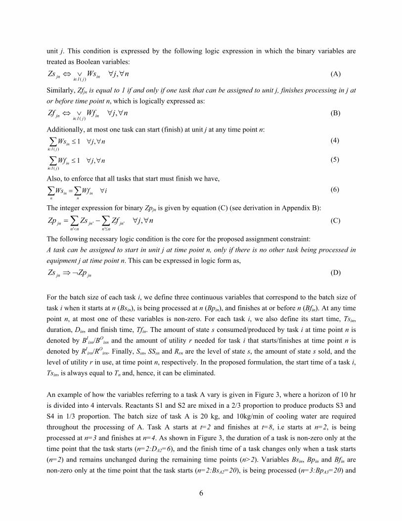
irn. Finally, Ssn, SSsn and Rrn are the level of state s, the amount of state s sold, and the level of utility r in use, at time point n, respectively. In the proposed formulation, the start time of a task i, Tsin, is always equal to Tn and, hence, it can be eliminated. An example of how the variables referring to a task A vary is given in Figure 3, where a horizon of 10 hr is divided into 4 intervals. Reactants S1 and S2 are mixed in a 2/3 proportion to produce products S3 and S4 in 1/3 proportion. The batch size of task A is 20 kg, and 10kg/min of cooling water are required throughout the processing of A. Task A starts at t=2 and finishes at t=8, i.e starts at n=2, is being processed at n=3 and finishes at n=4. As shown in Figure 3, the duration of a task is non-zero only at the time point that the task starts (n=2:DA2=6), and the finish time of a task changes only when a task starts (n=2) and remains unchanged during the remaining time points (n>2). Variables Bsin, Bpin and Bfin are non-zero only at the time point that the task starts (n=2:BsA2=20), is being processed (n=3:BpA3=20) and

7

finishes (n=4:BfA4=20), respectively. Similarly, the amount of utility reserved for task A (become available) is non-zero at the beginning (end) of the task at n=2 (n=4). In the example of Figure 3, 10kg/min of cooling water are reserved (“engaged”) for task A at n=2 (RI

A,CW,2 = 10) and become available again (“released”) at n=4 (RO

A,CW,4 = 10). Finally, the amount of a state consumed/produced by a task is non-zero when the task starts/finishes.

A

n 1 2 3 4 5Tn=TsAn 0 2 6 8 10DAn 0 6 0 0 0 TfAn 0 8 8 8 8

S340%

60% 75%S1

S2 S4

BOA,S3,4=5

BOA,S4,4=15

BsA2 = BpA3 = BfA4 = 20RI

A,CW,2 = ROA,CW,4 = 10

BIA,S1,2=8

BIA,S2,2=12

25%

6

Figure 3: Example of Tn, Tsin, Din, Tfin, RI

irn, ROirn, BI

isn and BOisn variables.

Regarding the time representation, we use the continuous-time representation I for tasks that produce at least one ZW-state; i.e. we require that the produced states of such a task are immediately transferred to another unit or to a storage tank. For all other tasks we use the continuous-time representation II, i.e. we allow them to finish within a period. For states with unlimited storage this is obviously not a restriction because the storage capacity and the timing of the transfer is not an issue. But this is also possible for FIS- and NIS- states because we assume that non-ZW-states can be temporarily stored in an equipment unit. If task A assigned to a unit U finishes at t=TfA (with Tn-1 < TfA < Tn), for example, and the storage tanks for the output states are full, unit U can be used for storage from t=TfA until t=Tn. When the states are actually transferred, at t=Tn, mass balance and storage capacity constraints are enforced and hence feasibility is guaranteed. If a solution where one unit is utilized as storage is suboptimal, a better solution can be obtained when additional time points are postulated allowing for all tasks performed in this unit to finish at exactly a time point. The proposed hybrid time representation, therefore, allows us to find the same solutions as continuous-time representation I using fewer time points whenever this is possible. Since the performance of continuous-time models depends heavily on the number of time points, the proposed mixed time representation leads to more efficient models. For each state s and time point n the mass balance and the storage constraints are,

1,)()(

1, >∀∀−+=+ ∑∑∈∈

− nsBBSSSSsIi

Iisn

sOi

Oisnnssnsn

(7)

nsCS ssn ∀∀≤ , (8)

where Cs is the capacity of the storage tank of state s. The continuous variable SSsn offers the possibility of removing final products before the end of the time horizon. This may be necessary if, for example, there is limited storage capacity for the final products. If this is not true or sales can occur only at the end of the horizon, as it is usually the case, variables SSsn can be fixed to zero for n<|N|. Constraint (7) can be modified to account for raw material purchases.

8

The total amount of utility r used at time point n is given by (9), and bounded not to exceed the maximum availability, Rr

MAX, by (10): nrRRRR

i

Iirn

i

Oirnrnrn ∀∀+−= ∑∑ −− ,11

(9)

nrRR MAXrrn ∀∀≤ , (10)

Since the batch size variables, Bsin, Bpin and Bfin, the start time Tsin, the duration, Din, the finish time, Tfin, the utility requirements, RI

irn/ROirn, as well as the consumption/production, BI

isn /BOisn, of state s are defined

for a task i and a time point n, we will first present the constraints for the calculation of those variables in disjunctive form, where each disjunction is expressed for all (i,n) pairs. For each (i,n) pair there are three different disjunctive cases: (a) task i starts (Wsin) at n, (b) is being processed (Wpin) at n, and (c) finishes (Wfin) at or before time point n. The disjunction in terms of the start of task i at time point n is given by disjunction (E) which is expressed for all n<|N|, since a task cannot start at the last time point,

Nni

RBBs

TfTfD

Ws

BpBsR

BsB

BfBpBsBBsB

DTsTfBsD

Ws

Iirn

Iisnin

inin

in

in

in

inirirIirn

inisIisn

ininin

MAXiin

MINi

ininin

iniiin

in

<∀∀

===

==

¬

∨

=+=

=

+=≤≤

+=+=

−++

,,

0

0

0

111

δγ

ρ

βα

(E)

As explained in Figure 3, if task i starts at time point n (Wsin is true), its duration Din, which is a linear function of Bsin, is non-zero while its finish time Tfin, changes by Din. The batch size Bsin, lies within lower and upper bounds and it is (a) equal to Bpin+1 if i is being processed at n+1 and (b) equal to Bfin+1 if i finishes at or before n+1. The amount of utility r reserved for task i, RI

irn, and the amount of state s consumed by task i, BI

isn, are also non-zero. If Wsin is false (¬Wsin) the condition that the finish time, Tfin, remains unchanged is enforced. This condition is not necessary, but our computational experience shows that it reduces the branch-and-bound tree size. The disjunction in terms of the processing of task i at time point n is given by (F). Note that if a task is processed at n it needs to start before n, and finish after n, which in turn implies that it cannot be processed at the first and the last time period.

9

NniBp

TfTfWp

RRD

BBBfBs

BfBpBpBpBsBpBBpB

TfTfWp

in

inin

in

Oirn

Iirnin

Oisn

Iisninin

ininin

ininin

MAXiin

MINi

inin

in

<<∀

=≥

¬∨

===

====

+=+=≤≤

=

−

++

−−

−

1,,0

0

0

1

11

11

1

(F)

When task i is being processed at n (i.e. Wpin is true), the finish time, Tfin, remains unchanged, the batch size Bpin lies within lower and upper bounds, and equals to the batch size of the previous and the next time points. If task i is not processed at n (¬Wpin), the finish time, Tfin, remains unchanged if i does not start at n (¬Wsin) and increases if task i starts at n (Wsin). The disjunction in terms of the finishing of task i at or before time point n is given by (G), which is expressed for all n>1, since a task cannot finish at the start of the scheduling horizon,

NniTfTf

Wf

BpBfR

BfB

BpBsBfBBfB

ZWiTTfZWiTTf

Wf

inin

in

in

inirirOirn

inisOisn

ininin

MAXiin

MINi

nin

nin

in

<∀∀

≥

¬∨

=+=

=

+=≤≤

∈=∉≤

−−−

,,

0

,,

111

δγ

ρ

(G)

Here, batch size Bfin lies within lower and upper bounds if task i finishes at or before time point n (Wfin), and it is equal to the batch size of the previous time period. The amount of state s produced, and the level or utility r becoming available are also non-zero. Finally, the proposed model, as most continuous-time models for the short-term scheduling of batch plants, appears to be effective when the objective function is the maximization of income or a profit/income related function,

∑∑=s n

sns SSZ ζmax (11)

The minimization of makespan (for fixed demand) can also be accommodated. The problem given by the mixed-integer constraints (1) – (11) and (C), the logic constraints (A), (B) and (D), and the disjunctions in (E), (F) and (G) corresponds to a hybrid GDP/MILP model, which as will be shown in the next section will be transformed into an MILP model.

10

4.2. MILP Model Using the definitions of the binaries Wsin, Wpin, Wfin, Zsin, Zpin, and Zfin, we can transform the logic conditions (A), (B) and (D), and the disjunctions in (E) – (G) into mixed-integer constraints. As explained in Appendix B, the binaries Zsjn, Zpjn, Zfjn and Wpin can be expressed through binaries Wsin and Wfin, which are the only ones used in the mixed-integer constraints. Assignment Constraints The basic assignment constraint (12) is derived in Appendix B and follows from the constraints in (A) – (D). Constraints (13) and (14) enforce the conditions that no task can finish at t=0 or start at the end of the horizon. Constraints (4) – (6) are repeated for completeness.

njWsjIi

in ∀∀≤∑∈

,1)(

(4)

njWfjIi

in ∀∀≤∑∈

,1)(

(5)

iWfWsn

inn

in ∀=∑∑ (6)

njWfWsjIi nn

inin ∀∀≤−∑ ∑∈ ≤

,1)()( '

'' (12)

iWfi ∀= 00 (13)

NniWsin =∀= ,0 (14)

Duration, finish time and time-matching constraints From the disjunction in (E) the duration of a task is calculated by equation (15) using convex hull reformulation (Balas, 1985; Raman and Grossmann, 1994) and eliminating variables, while the finish time is expressed with big-M constraints (16) and (17) which are active only if task i starts at time point n (Wsin=1):

niBsWsD iniiniin ∀∀+= ,βα (15)

niWsHDTsTf inininin ∀∀−++≤ ,)1( (16)

niWsHDTsTf inininin ∀∀−−+≥ ,)1( (17)

As explained in Figure 3 and enforced in the disjunction in (E), the finish time, Tfin, of a task i remains unchanged until the next occurrence of task i. This condition is enforced by the big-M constraint in (18). Constraint (19) is used to enforce that, (a) Tfin is always greater or equal to Tfin-1, and (b) the “step” in the finish time, Tfin, when a task occurs at time n, must be at least as large as the duration of task i. The latter condition is not necessary and it is not derived from disjunction (E), but its addition leads to smaller branch-and-bound trees and shorter computational times:

niWsHTfTf ininin ∀∀⋅≤− − ,1 (18)

niDTfTf ininin ∀∀≥− − ,1 (19)

11

Since start time, Tsin, is equal to Tn variables Tsin are eliminated [constraint (20)]. Constraints (21) and (22) are the time-matching constraints for the finish time, Tfin, of a task and result from disjunction (G) using the big-M formulation. Note that in the general case, a task i may finish at or before time point n [constraint (21)], but when it produces a material for which a Zero-Wait (ZW) storage policy applies the finish time of task i should coincide with time point n [effect of constraints (21) and (22)]:.

niTTs nin ∀∀= , (20)

niWfHTTf innin ∀∀−+≤− ,)1(1 (21)

nZWIiWfHTTf innin ∀∈∀−−≥− ,)1(1 (22)

An example of how variables Tn, Tsin and Tfin vary for a task A is given in Figure 4. Note that task A is assumed to produce a state for which ZW storage policy applies, so the finish time must coincide with a time point. Although integer processing times have been used, the same principles apply for real constant or variable processing times. As shown, start and finish times are defined for seven time points and the first are always equal to Tn, and thus eliminated. Due to constraint (18), TfA2 and TfA3 are equal to 3 (i.e. equal to TfA1) and TfA6 and TfA7 are equal to 9 (i.e. equal to TfA5), while constraint (19) is trivially satisfied: TfA4 - TfA3 = 7 – 3 = 4 ≥ 3 = DA4 and TfA5 - TfA4 = 9 – 7 = 2 ≥ 2 = DA5.

A

t 0 1 2 3 4 5 6 7 8 9 10n 0 1 2 3 4 5 6 7 Tn=TsAn 0 1 2 3 3 7 9 10DAn 0 2 0 0 3 2 0 0 TfAn 0 3 3 3 7 9 9 9

A A

Figure 4: Relationships among Tn, Tsin, Tfin and Din variables.

Batch size constraints Constraints (23) to (24) impose minimum and maximum bounds on the batch size of a task and result from the convex hull reformulation of disjunctions (E), (F) and (G). Note that the term multiplied with Bi

MIN and BiMAX in constraint (25) is equal to the auxiliary binary Wpin (Appendix B). Constraint (26)

enforces that variables Bsin, Bpin and Bfin are equal for a given task, and it is also derived from disjunctions (E) – (G) using the convex hull reformulation and eliminating the disaggregated variables:

niWsBBsWsB inMAXiinin

MINi ∀∀≤≤ , (23)

niWfBBfWfB inMAXiinin

MINi ∀∀≤≤ , (24)

niWfWsBBpWfWsBnn

innn

inMAXiin

nnin

nnin

MINi ∀∀−≤≤− ∑∑∑∑

≤<≤<

,)()('

''

''

''

' (25)

niBfBpBpBs inininin ∀∀+=+ −− ,11 (26)

12

The amount of state s consumed/produced by task i at time point n is calculated through equation (27)/(29) and bounded by equation (28)/(30), where SI(i) and SO(i) are the set of input and output states of task i, respectively. Constraints (28) and (30) are not necessary, but result in shorter computational times. The convex hull reformulation was used for the derivation of constraints (27) – (30).

)(,, iSIsniBsB inisIisn ∈∀∀∀= ρ (27)

)(,, iSIsniWsBB inisMAXi

Iisn ∈∀∀∀≤ ρ (28)

)(,, iSOsniBfB inisOisn ∈∀∀∀= ρ (29)

)(,, iSOsniWfBB inisMAXi

Oisn ∈∀∀∀≤ ρ (30)

Mass balance/Storage constraints As shown above, constraints (7) and (8) express the mass balance and capacity constraints for state s at time point n:

1,)()(

1, >∀∀−+=+ ∑∑∈∈

− nsBBSSSSsIi

Iisn

sOi

Oisnnssnsn

(7)

nsCS ssn ∀∀≤ , (8)

Utility constraints The amount of utility r consumed by task i that starts at time point n is calculated through equation (31); the amount of utility r released at the end of task i is calculated through equation (32). Constraints (31) and (32) are derived from disjunctions (E) and (G), respectively, using the convex hull reformulation. The total amount of utility r consumed by various tasks during period n is calculated by equation (9) and bounded not to exceed Rr

MAX by constraint (10): nriBsWsR inirsinir

Iirn ∀∀∀+= ,,δγ (31)

nriBfWfR inirsinirOirn ∀∀∀+= ,,δγ (32)

nrRRRRi

Iirn

i

Oirnrnrn ∀∀+−= ∑∑ −− ,11

(9)

nrRR MAXrrn ∀∀≤ , (10)

Objective function

As in the hybrid GDP/MILP model, the objective is given by,

∑∑=s n

sns SSZ ζmax (11)

Wsin, Wfin ∈ {0,1}, Bsin, Bpin, Bfin, SSsn, Ssn, Tn, Tfin, Din, BIisn, BO

isn RIirn, RO

irn, Rrn ≥ 0 (33) Constraints (1) – (33) comprise the MILP model (M) for the short-term scheduling of multipurpose batch plants. This model can be tightened by adding the following valid inequalities that lead to model (M*).

13

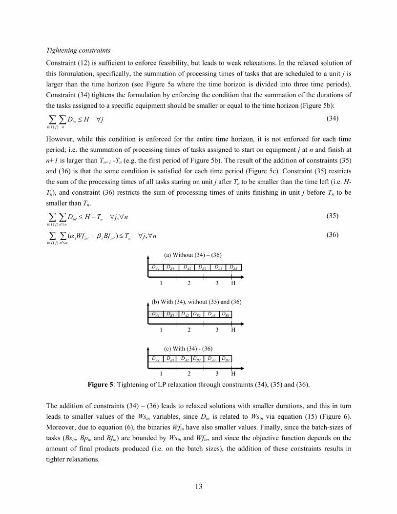
Tightening constraints

Constraint (12) is sufficient to enforce feasibility, but leads to weak relaxations. In the relaxed solution of this formulation, specifically, the summation of processing times of tasks that are scheduled to a unit j is larger than the time horizon (see Figure 5a where the time horizon is divided into three time periods). Constraint (34) tightens the formulation by enforcing the condition that the summation of the durations of the tasks assigned to a specific equipment should be smaller or equal to the time horizon (Figure 5b):

∑ ∑∈

∀≤)( jIi n

in jHD (34)

However, while this condition is enforced for the entire time horizon, it is not enforced for each time period; i.e. the summation of processing times of tasks assigned to start on equipment j at n and finish at n+1 is larger than Tn+1 -Tn (e.g. the first period of Figure 5b). The result of the addition of constraints (35) and (36) is that the same condition is satisfied for each time period (Figure 5c). Constraint (35) restricts the sum of the processing times of all tasks staring on unit j after Tn to be smaller than the time left (i.e. H-Tn), and constraint (36) restricts the sum of processing times of units finishing in unit j before Tn to be smaller than Tn.

∑ ∑∈ ≥

∀∀−≤)( '

' ,jIi

nnn

in njTHD (35)

∑ ∑∈ ≤

∀∀≤+)(

''

' ,)(jIi

nininn

ini njTBfWf βα (36)

DA1 DB1 DA2 DB2 DA3 DB3

1 2 3 H

(a) Without (34) – (36)

DA1 DB1 DA2 DB2 DA3 DB3

1 2 3 H

(b) With (34), without (35) and (36)

DA1 DB1 DA2 DB2 DA3 DB3

1 2 3 H

(c) With (34) - (36)

Figure 5: Tightening of LP relaxation through constraints (34), (35) and (36).

The addition of constraints (34) – (36) leads to relaxed solutions with smaller durations, and this in turn leads to smaller values of the Wsin variables, since Din is related to Wsin via equation (15) (Figure 6). Moreover, due to equation (6), the binaries Wfin have also smaller values. Finally, since the batch-sizes of tasks (Bsin, Bpin and Bfin) are bounded by Wsin and Wfin, and since the objective function depends on the amount of final products produced (i.e. on the batch sizes), the addition of these constraints results in tighter relaxations.

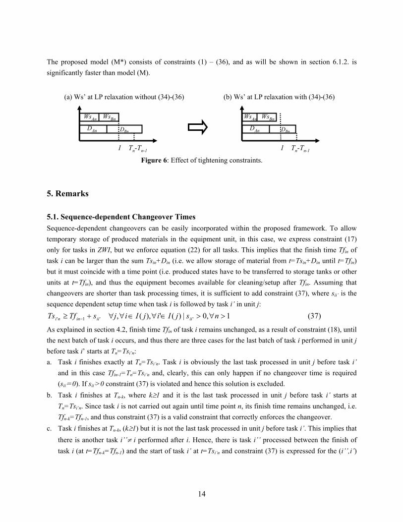
14

The proposed model (M*) consists of constraints (1) – (36), and as will be shown in section 6.1.2. is significantly faster than model (M).

WsAn WsBn

DBnDAn

1 Tn-Tn-1

(a) Ws’ at LP relaxation without (34)-(36) (b) Ws’ at LP relaxation with (34)-(36)

WsAn WsBn

DBnDAn

1 Tn-Tn-1 Figure 6: Effect of tightening constraints.

5. Remarks 5.1. Sequence-dependent Changeover Times Sequence-dependent changeovers can be easily incorporated within the proposed framework. To allow temporary storage of produced materials in the equipment unit, in this case, we express constraint (17) only for tasks in ZWI, but we enforce equation (22) for all tasks. This implies that the finish time Tfin of task i can be larger than the sum Tsin+Din (i.e. we allow storage of material from t=Tsin+Din until t=Tfin) but it must coincide with a time point (i.e. produced states have to be transferred to storage tanks or other units at t=Tfin), and thus the equipment becomes available for cleaning/setup after Tfin. Assuming that changeovers are shorter than task processing times, it is sufficient to add constraint (37), where sii’ is the sequence dependent setup time when task i is followed by task i’ in unit j:

1,0|)('),(, ''1' >∀>∈∀∈∀∀+≥ − nsjIijIijsTfTs iiiiinni (37)

As explained in section 4.2, finish time Tfin of task i remains unchanged, as a result of constraint (18), until the next batch of task i occurs, and thus there are three cases for the last batch of task i performed in unit j before task i’ starts at Tn=Tsi’n: a. Task i finishes exactly at Tn=Tsi’n. Task i is obviously the last task processed in unit j before task i’

and in this case Tfin-1=Tn=Tsi’n and, clearly, this can only happen if no changeover time is required (sii’=0). If sii’>0 constraint (37) is violated and hence this solution is excluded.

b. Task i finishes at Tn-k, where k≥1 and it is the last task processed in unit j before task i’ starts at Tn=Tsi’n. Since task i is not carried out again until time point n, its finish time remains unchanged, i.e. Tfn-k=Tfn-1, and thus constraint (37) is a valid constraint that correctly enforces the changeover.

c. Task i finishes at Tn-k, (k≥1) but it is not the last task processed in unit j before task i’. This implies that there is another task i’’≠ i performed after i. Hence, there is task i’’ processed between the finish of task i (at t=Tfn-k=Tfn-1) and the start of task i’ at t=Tsi’n and constraint (37) is expressed for the (i’’,i’)

15

pair as well. Since we have assumed that setup times are smaller than the processing times constraint (37) for the (i’’,i’) pair is tighter than constraint (37) for the (i’,i) pair, and the latter is redundant.

Note that no additional variables are needed to model sequence dependent changeover times. The requirement to apply continuous-time representation I for all tasks, however, results to models that are difficult to solve due to the increased number of time points. It should also be mentioned that if in addition to changeover times one would like to include changeover costs this would require the introduction of the new variable Yii’n that is equal to 1 if task i, finishing at or before time point n, is followed by task i’, starting at time point n, where i∈I(j) and i’∈I(j) for some unit j. Variable Yii’n is defined only for pairs of tasks that take place in the same unit and have nonzero changeover cost; it can be treated as a continuous variable because it will always be equal to 0 or 1 in an integer solution and is activated through the following constraint (assuming that changeover times are smaller than processing times):

||1,0|)('),(,1 ''1' NnjIijIijWsWfY iiniinnii <<>∈∀∈∀∀−+≥ − κ (38)

The objective function is modified as follows,

∑ ∑ ∑ ∑∑∑<< ∈ ∈

−=||1 )( )('

''maxNn j jIi jIi

niiiis n

sns YSSZ κζ (11*)

where κii’ is the changeover cost for the changeover from task i to task i’. If variable Yii’n is included, we can also tighten valid inequalities (34)-(36) as follows:

∑ ∑ ∑ ∑∑∈ << ∈ ∈

∀≤+)( ||1 )( )('

''jIi Nn jIi jIi

niiiin

in jHYsD (34*)

∑ ∑ ∑ ∑∑∈ > ∈ ∈≥

∀∀−≤+)( ' )( )('

''''

' ,jIi

nnn jIi jIi

niiiinn

in njTHYsD (35*)

∑ ∑ ∑ ∑∑∈ ≤ ∈ ∈≤

∀∀≤++)( ' )( )('

'''''

' ,)(jIi

nnn jIi jIi

niiiiininn

ini njTYsBfWf βα (36*)

5.2. Shared Storage Tanks The proposed model can also be extended to account for storage tanks shared among many states, a feature very common in chemical plants. To do so we need to treat a shared storage tank s as a unit j. For each state that can be stored to tank j (i.e. s∈S(j)) we define a new binary variable Vjsn that is 1 is state s is stored in tank j during period n. If JT is the set of shared storage tanks and Cj is the capacity of storage tank j, the following two constraints are added:

nJTjVjSs

jsn ∀∈∀≤∑∈

,1)(

(38)

njSsJTjVCS jsnjsn ∀∈∀∈∀≤ ),(, (39)

Constraint (38) ensures that at most one state is stored in tank j at any time, and constraint (39) ensures that the inventory of state s at time point n is zero if binary Vjsn is zero. In some cases it is computationally more efficient to model variables Vjsn as Special Ordered Sets of type I (SOS1) variables and express constraint (39) as equality. Finally, if state s can be stored in more than one tank, constraint (39) is

16

expressed for variable Ssjn which denotes the amount of state s at time n stored in tank j, and constraint (40) is added:

nSsSSsJTj

sjnsn ∀∈∀= ∑∈

*,)(

(40)

where S* is the set of states for which there is no dedicated storage and JT(s) is the set of storage tanks in which state s can be stored. It is important to note that the addition of binary variables Vjsn, and constraints (38) and (39) result to a larger and more difficult to solve MILP model. 5.3. Number of Time Points The choice of number of intervals is an important issue for all continuous-time STN/RTN models. A rigorous approach was proposed by Zhang and Sargent (1996), but as the authors indicate, the bounds on the number of intervals are very loose. In this work we use the approach used in practically all continuous STN models, where we start with a small number of intervals and we iteratively increase the number of intervals by one until there is no improvement in the objective function for a fixed number of iterations (usually one or two). 5.4. Minimization of Makespan If the objective is to minimize the makespan, MS, for fixed demand, the following changes need to be made in the MILP model (M*): (a) The objective function is, MSmin (11’)

(b) Addition of constraint (41) that enforces that the demand is met,

sdSS sn

sn ∀≥∑ or sdSS sn

sn ∀=∑ (41)

where ds is the demand for state s at the end of the horizon. (c) The length of the fixed time horizon, H, is replaced by the makespan, MS, in constraints (2), (34) and

(35). The parameter H is used in constraints (16), (17), (18), (21) and (22) as an overestimate of the makespan.

The model for minimization of makespan consists of equations (1) – (10), (11’) and (12) – (36) and (41). As in all STN models, the computational efficiency of the proposed model decreases when the objective is the minimization of makespan. The minimization of makespan for a fixed demand, however, is more common in short-term scheduling. We are currently working on the development of a scheduling framework that combines Mixed-Integer Programming and Constraint Programming (CP) techniques that successfully addresses the problem of makespan minimization (Maravelias and Grossmann, 2003a). Finally, it should be noted that the proposed model can be extended to handle delivery and due dates (see Maravelias and Grossmann, 2003b).

17

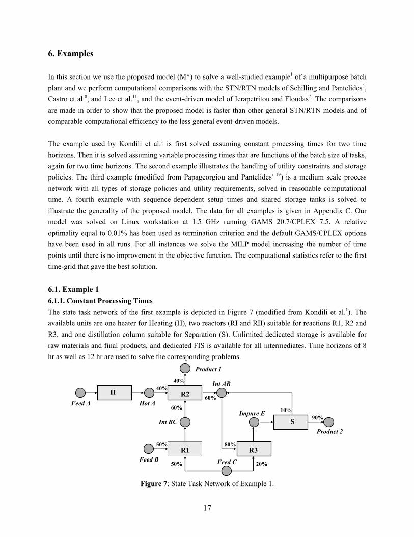
6. Examples In this section we use the proposed model (M*) to solve a well-studied example1 of a multipurpose batch plant and we perform computational comparisons with the STN/RTN models of Schilling and Pantelides4, Castro et al.8, and Lee et al.11, and the event-driven model of Ierapetritou and Floudas7. The comparisons are made in order to show that the proposed model is faster than other general STN/RTN models and of comparable computational efficiency to the less general event-driven models. The example used by Kondili et al.1 is first solved assuming constant processing times for two time horizons. Then it is solved assuming variable processing times that are functions of the batch size of tasks, again for two time horizons. The second example illustrates the handling of utility constraints and storage policies. The third example (modified from Papageorgiou and Pantelidesi 19) is a medium scale process network with all types of storage policies and utility requirements, solved in reasonable computational time. A fourth example with sequence-dependent setup times and shared storage tanks is solved to illustrate the generality of the proposed model. The data for all examples is given in Appendix C. Our model was solved on Linux workstation at 1.5 GHz running GAMS 20.7/CPLEX 7.5. A relative optimality equal to 0.01% has been used as termination criterion and the default GAMS/CPLEX options have been used in all runs. For all instances we solve the MILP model increasing the number of time points until there is no improvement in the objective function. The computational statistics refer to the first time-grid that gave the best solution. 6.1. Example 1 6.1.1. Constant Processing Times The state task network of the first example is depicted in Figure 7 (modified from Kondili et al.1). The available units are one heater for Heating (H), two reactors (RI and RII) suitable for reactions R1, R2 and R3, and one distillation column suitable for Separation (S). Unlimited dedicated storage is available for raw materials and final products, and dedicated FIS is available for all intermediates. Time horizons of 8 hr as well as 12 hr are used to solve the corresponding problems.

Feed A

HHot A

R2

Product 1

R1Feed B Feed C

R3

Impure ES

Product 2

Int AB

Int BC

40%40%

60%

60%

50%

50% 20%

80%

10%90%

Figure 7: State Task Network of Example 1.

18

When the time horizon is 8 hours, the optimal solution with a profit of $1,917.5 is found with 6 time points (5 intervals). The Gantt chart of the units and the batch-sizes of the optimal solution are shown in Figure 8. When the time horizon is 12 hours, the optimal solution of $3,638.8 is found using 8 time points. The Gantt chart of the optimal solution is given Figure 9. The model and solution statistics are given in Table 1.

HeaterReactor IReactor IIDist. Col

H/52

R1/78

R2/50

R2/80 R1/78

R3/48 R2/50

R2/80

S/97.5

0 2 4 6 8 t (hr)

H/100

R3/50

Figure 8: Gantt chart for the optimal solution of proposed model for H=8 hr (6 time points).

HeaterReactor IReactor IIDist. Col

H/52

R1/80R2/50R2/80 R1/80

R3/50 R2/50R2/80S/130

0 2 4 6 8 10 12 t (hr)

H/20

R3/80R1/50 R2/50

H/68R3/50R3/69 R2/40

S/118.8

Figure 9: Gantt chart for the optimal solution of model (M*) for H=12 hr (8 time points)

Table 1: Model and Solution Statistics of model (M*) for Example 1 for constant processing times.

H = 8 H = 12 Time points (events) 6 8 Binary variables 96 128 Continuous variables 657 875 Constraints 1431 1903 LP relaxation 2473.8 3799.4 Objective ($) 1917.5 3638.8 Nodes 271 239 CPU Time (sec) 0.72 1.68

6.1.2. Variable Processing Times The previous example is also solved assuming variable processing times. The optimal solution for the 8-hour time horizon is $1,498.6 and is found using 5 time points. The equipment Gantt chart of the optimal solution is shown in Figure 10 (where the batch-size and duration of each task are reported). Compared to the optimal solution with constant processing times (Figure 8) we observe that while the batch sizes are smaller, the processing times are longer; this is due to the fact that for all tasks the processing time for the maximum capacity corresponds to a processing time that is 33% longer than the constant processing time of Figure 8. The batch of reaction R1 in reactor RII, for example, has a batch-size equal to 64.812 and a processing time equal to 2.413 hours, while in Figure 8 it has a larger batch-size (78 kg) and a smaller

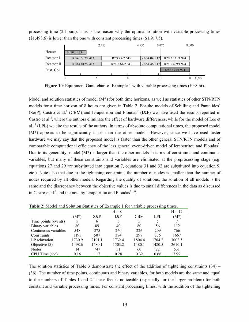
19

processing time (2 hours). This is the reason why the optimal solution with variable processing times ($1,498.6) is lower than the one with constant processing times ($1,917.5).

0 2 4 6 8 t (hr)

H/100/1.334

R1/40.507/2.413 R2/45.4/2.543 R3/34.04/1.12 R2/22.131/1.924

HeaterReactor IReactor IIDist. Col

R1/64.812/2.413 R2/72.61/2.543 R3/54.46/1.12 R2/35.409/1.924

S/88.494/1.924

2.413 4.956 6.076 8.000

Figure 10: Equipment Gantt chart of Example 1 with variable processing times (H=8 hr).

Model and solution statistics of model (M*) for both time horizons, as well as statistics of other STN/RTN models for a time horizon of 8 hours are given in Table 2. For the models of Schilling and Pantelides4 (S&P), Castro et al.8 (CBM) and Ierapetritou and Floudas7 (I&F) we have used the results reported in Castro et al.8, where the authors eliminate the effect of hardware differences, while for the model of Lee et al.11 (LPL) we cite the results of the authors. In terms of absolute computational times, the proposed model (M*) appears to be significantly faster than the other models. However, since we have used faster hardware we may say that the proposed model is faster than the other general STN/RTN models and of comparable computational efficiency of the less general event-driven model of Ierapetritou and Floudas7. Due to its generality, model (M*) is larger than the other models in terms of constraints and continuous variables, but many of these constraints and variables are eliminated at the preprocessing stage (e.g. equations 27 and 29 are substituted into equation 7, equations 31 and 32 are substituted into equation 9, etc.). Note also that due to the tightening constraints the number of nodes is smaller than the number of nodes required by all other models. Regarding the quality of solutions, the solution of all models is the same and the discrepancy between the objective values is due to small differences in the data as discussed in Castro et al.8 and the note by Ierapetritou and Floudas21, ii. Table 2: Model and Solution Statistics of Example 1 for variable processing times.

H = 8 H = 12 (M*) S&P I&F CBM LPL (M*) Time points (events) 5 6 5 5 5 7 Binary variables 80 89 40 80 56 112 Continuous variables 548 375 260 226 209 766 Constraints 1195 507 374 297 376 1667 LP relaxation 1730.9 2191.1 1732.4 1804.4 1704.2 3002.5 Objective ($) 1498.6 1480.1 1503.2 1480.1 1480.5 2610.1 Nodes 14 747 51 60 22 531 CPU Time (sec) 0.16 117 0.28 0.32 0.66 3.99

The solution statistics of Table 3 demonstrate the effect of the addition of tightening constraints (34) – (36). The number of time points, continuous and binary variables, for both models are the same and equal to the numbers of Tables 1 and 2. The effect is noticeable (especially for the larger problem) for both constant and variable processing times. For constant processing times, with the addition of the tightening

20

constraints, the gap between the LP relaxation and the optimal solution is reduced by 8-11% and for variable processing times the gap is closed by 32-46%. In both cases the number of nodes is reduced by a factor of 2 to 5. Note also that the improvement in computational time is larger as the problem size increases. Table 3: Computational impact of tightening constraints (34) – (36).

Constant Processing Times Variable Processing Times H = 8 H = 12 H = 8 H = 12 (M) (M*) (M) (M*) (M) (M*) (M) (M*) Constraints 1379 1431 1835 1903 1151 1195 1607 1667 LP relaxation 2541.9 2473.8 3813.2 3799.4 1931.6 1730.9 3190.5 3002.5 Objective ($) 1917.5 1917.5 3638.8 3638.8 1498.6 1498.6 2610.1 2610.1 Nodes 753 271 1224 239 29 14 2649 531 CPU Time (sec) 1.16 0.72 7.1 1.68 0.14 0.16 7.58 3.99

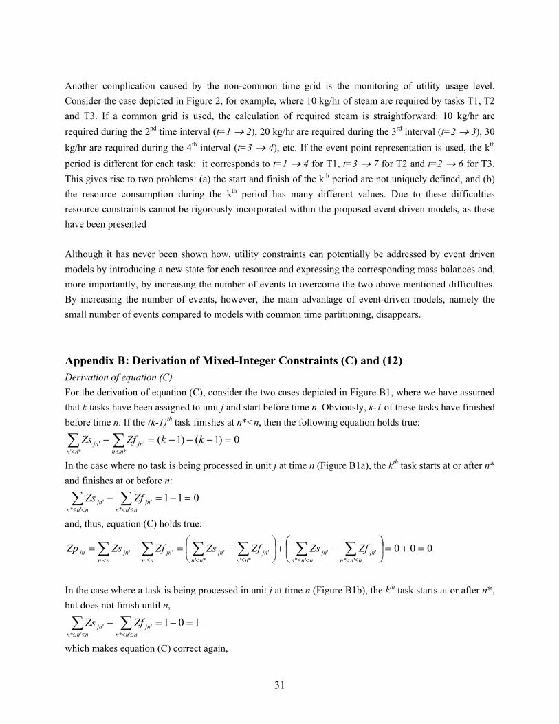
6. 2. Example 2 To illustrate the handling of utility constraints we consider the state task network of Figure 11 (data in Appendix C). There are two types of reactors available for the process (type I and II) with different number of corresponding units available: two reactors (RI1 and RI2) of type I, while one reactor (RII) of type II. Reactions R1 and R2 require type I reactor, while reactions R3 and R4 require type II reactor. Furthermore, reactions R1 and R3 require heat, provided by steam (HS) produced in limited amounts in the plant, while reactions R2 and R4 are exothermic and require cooling water (CW), also available in limited amounts. Due to safety reasons and temperature restrictions, the heat integration of the process is not possible. Utility requirements include a fixed term as well as a variable term proportional to the batch-size. The minimum batch-size for all tasks is half the capacity of the unit where they take place. Processing times for all tasks are functions of the batch-size. Specifically, the minimum batch size is processed in 60% of the time needed for the maximum batch-size. There is unlimited storage for the raw materials and final products and finite capacity for intermediates I1, I2 and I3.

R1

R2 R4

R380%

20%

70%

40%

60%30%

R1

R2

I1

I2

I3P1

P2

Figure 11: State Task Network of Example 2.

6.2.1. Maximization of Profit To illustrate how the availability of such resources can alter the solution of a problem, we consider two cases. We first solve this problem assuming that the availability of both steam and cooling water is 40 kg/min (case 1). The optimal profit in this case is $5,904.0. The Gantt chart of units and the plot showing the level of utilization of steam and cooling water at the optimal solution are given in Figure 12. Then we

21

solve the problem assuming that the availability of utilities is 30 kg/min (case 2), which yields the solution shown in Figure 12 with a profit of $5,227.8. Note that we have plotted the resource consumption level calculated by the model which is not necessarily equal to the actual consumption level. In Figure 12, for example, the consumption of cooling water is not constant throughout the second period, because task R2 finishes before the end of the second period. This discrepancy is due to the fact that we use the second continuous-time representation for tasks that do not produce ZW states, allowing for a task to finish within a time period while the resource consumption is constant throughout a period (constraints (9), (10), (31) and (32)). This assumption, however, does not compromise feasibility or optimality. Specifically, if a task finishes before a time point, the calculated resource consumption for this period will be an overestimation and is obviously feasible. Moreover, if another solution (that uses the extra resource amount) was better than the existing one, this solution would be found if one or more additional time points are used; if no better solution can be obtained, this means that the existing overestimated solution corresponds to the best feasible solution. For the problem of Figure 12, for instance, no better solution is found when we re-solve the problem with 8 or 9 time points; i.e. the utilization of the extra resource at the end of the second period does not yield a better solution.

RI1RI2RII

0 2 4 6 8 t (hr)

0 2 4 6 8 t (hr)

RMAX

HSCW

R2-40R2-46.4

R1-40 R1-49.6 R1-40

R4-72 R3-40 R3-60.8

(kg/min)

40

20

Figure 12: Solution of example 2 for maximization of profit (case 1).

RI1RI2RII

0 2 4 6 8 t (hr)

R2-40 R1-40

R2-36.4

R1-50.8

R4-47.7 R4-41.7R3-55

(kg/min)

30

20

10

0 2 4 6 8 t (hr)

RMAX

HSCW

Figure 13: Solution of example 2 for maximization of profit (case 2).

22

In case 1, 100.8 kg of P1 and 72.0 kg of P2 are produced. As shown in Figure 12, the level of utilization of steam during the fifth interval is 40 kg/min and the level of consumption of cooling water during the first, third and fourth interval are above 30 kg/min. Thus, when the maximum availability of steam and water is 30 kg/min this solution is not feasible. As shown in Figure 13 for case 2, to keep the level of utilization of cold water bellow 30 kg/min during the first interval, the batch-size of task R1 that is performed in reactor RI2 is reduced to 36.7 kg. Similarly, during the third period the batch size of reaction R4 (performed in reactor RII) is reduced to 47.7 kg (compared to 72 kg of case 1). Furthermore, to keep the consumption of steam bellow 30kg/min, there are only two batches of reaction R1 (instead of three) in reactor RI1, and a second batch of R4 instead of two batches of reaction R3. In the optimal solution of case 2, 55 kg of P1 and 89.4 kg of P2 are produced. Note that if the availability of both utilities is reduced to 25 kg/min, the optimal profit reduces to $4,537, and if it is further decreased to 20 kg/min no final products can be produced. Model and solution statistics for both cases are given in Table 4. 6.2.2. Minimization of Makespan The two above cases are resolved for a fixed demand of 100 kg of P1 and 80 kg of P2, using the minimization of makespan as objective function. An upper bound on the makespan of 15 hr (H=15) has been used for constraints (16)-(18), (21) and (22). When the availability of resources is 40 kg/min the makespan is 8.5 hr. The equipment Gantt chart and the utility consumption graph are shown in Figure 14. When the availability of resources is reduced to 30 kg/min the optimal makespan is 9.025 hr, and the equipment Gantt chart and the utility consumption graph for this case are shown in Figure 15. Comparing the two Gantt charts, we observe that in the second case several tasks are delayed due to the reduced utility availability. Model and solution statistics for both cases are given in Table 4 where it can be seen that the minimization of makespan requires greater computational effort.

RI1RI2RII

0 2 4 6 8 t (hr)

R2-40R2-25

R1-40

(kg/min)

40

20

0 2 4 6 8 t (hr)

R2-25R1-52 R1-40

R3-60R3-40R4-40 R4-40

RMAX

HSCW

Figure 14: Solution of example 2 for minimization of makespan (case 1).

23

RI1RI2RII

0 2 4 6 8 t (hr)

R2-40R2-25 R2-25

R1-40 R1-40 R1-40

R3-45 R4-40 R4-40 R3-55

(kg/min)

30

20

10

0 2 4 6 8 t (hr)

RMAX

HSCW

Figure 15: Solution of example 2 for minimization of makespan (case 2).

Table 4: Model and solution statistics of example 2.

Max Profit Min Makespan Case 1 Case 2 Case 1 Case 2 Time points (events) 7 6 8 7 Binary variables 84 72 96 84 Continuous variables 661 567 753 659 Constraints 1,335 1,146 1,528 1,339 LP relaxation 8,875.4 7,685.7 5.077 5.077 Objective $5,904.0 $5,227.8 8.5 hr 9.025 hr Nodes 632 97 2,682 489 CPU Time (sec) 1.98 0.34 8.99 1.66

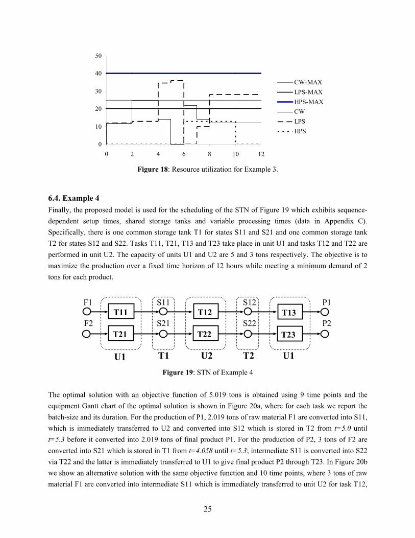
6.3. Example 3 The proposed model is used for the scheduling of the STN shown in Figure 16, which is a modification of an example of Papageorgiou and Pantelides (1996) (data in Appendix C). A time horizon of 12 hr is used. The plant consists of 6 units: Unit 1 for tasks T1 and T4, Unit 2 for T2, Unit 3 for T3, Unit 4 for T5 and T6, Unit 5 for T7 and T9, and Unit 6 for T8 and T10. Unlimited storage is available for raw materials F1 and F2, intermediate Int1 and Int2 and final products P1, P2 and P3, finite storage is available for states S3 and S4, no intermediate storage is available for states S2 and S6 and zero-wait policy applies for states S1 and S5. Tasks T2, T7, T9 and T10 require cooling water (CW), tasks T1, T3, T5 and T8 require low pressure steam (LPS), while tasks T4 and T6 require high pressure steam (HPS). No heat integration is possible. The maximum availability of cooling water and low and high pressure steam is 25, 40 and 20 kg/min, respectively. Solving the proposed MILP model (M*) yields the equipment Gantt chart shown in Figure 17 and the graph of resource utilization shown in Figure 18. The optimal solution is $13,000 and eight intervals (nine time points) are needed to obtain it. As shown in the Gantt chart of Figure 17, tasks T1 and T7 are immediately followed by tasks T2 and T8, respectively, because they produce states S1 and S5 for which zero-wait policy applies. Note that for task T2 this is not necessary because S2 can remain in the unit before it is sent to the next task (NIS), whereas for the final

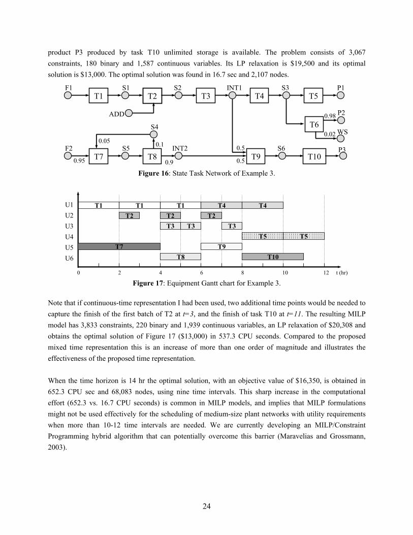
24

product P3 produced by task T10 unlimited storage is available. The problem consists of 3,067 constraints, 180 binary and 1,587 continuous variables. Its LP relaxation is $19,500 and its optimal solution is $13,000. The optimal solution was found in 16.7 sec and 2,107 nodes.

T1 T2 T3 T4 T5

T7 T8

T6

T9 T10

F1 S1 S2 INT1 S3 P1

P2

WS

P3F2 S5 INT2

S4

ADD

S6

0.95

0.05 0.1

0.9 0.5

0.5

0.98

0.02

Figure 16: State Task Network of Example 3.

U1U2U3U4U5U6

0 2 4 6 8 10 12 t (hr)

T1 T1 T1T2T2 T2T3 T3 T3

T4

T5

T4

T7T8

T9T10

T5

Figure 17: Equipment Gantt chart for Example 3.

Note that if continuous-time representation I had been used, two additional time points would be needed to capture the finish of the first batch of T2 at t=3, and the finish of task T10 at t=11. The resulting MILP model has 3,833 constraints, 220 binary and 1,939 continuous variables, an LP relaxation of $20,308 and obtains the optimal solution of Figure 17 ($13,000) in 537.3 CPU seconds. Compared to the proposed mixed time representation this is an increase of more than one order of magnitude and illustrates the effectiveness of the proposed time representation. When the time horizon is 14 hr the optimal solution, with an objective value of $16,350, is obtained in 652.3 CPU sec and 68,083 nodes, using nine time intervals. This sharp increase in the computational effort (652.3 vs. 16.7 CPU seconds) is common in MILP models, and implies that MILP formulations might not be used effectively for the scheduling of medium-size plant networks with utility requirements when more than 10-12 time intervals are needed. We are currently developing an MILP/Constraint Programming hybrid algorithm that can potentially overcome this barrier (Maravelias and Grossmann, 2003).

25

0

10

20

30

40

50

0 2 4 6 8 10 12

CW-MAXLPS-MAXHPS-MAXCWLPSHPS

Figure 18: Resource utilization for Example 3.

6.4. Example 4 Finally, the proposed model is used for the scheduling of the STN of Figure 19 which exhibits sequence-dependent setup times, shared storage tanks and variable processing times (data in Appendix C). Specifically, there is one common storage tank T1 for states S11 and S21 and one common storage tank T2 for states S12 and S22. Tasks T11, T21, T13 and T23 take place in unit U1 and tasks T12 and T22 are performed in unit U2. The capacity of units U1 and U2 are 5 and 3 tons respectively. The objective is to maximize the production over a fixed time horizon of 12 hours while meeting a minimum demand of 2 tons for each product.

F1 S11 S12 P1

F2 S21 S22 P2T11

T21

T12

T22

T13

T23

U2 U1U1 T1 T2

Figure 19: STN of Example 4 The optimal solution with an objective function of 5.019 tons is obtained using 9 time points and the equipment Gantt chart of the optimal solution is shown in Figure 20a, where for each task we report the batch-size and its duration. For the production of P1, 2.019 tons of raw material F1 are converted into S11, which is immediately transferred to U2 and converted into S12 which is stored in T2 from t=5.0 until t=5.3 before it converted into 2.019 tons of final product P1. For the production of P2, 3 tons of F2 are converted into S21 which is stored in T1 from t=4.058 until t=5.3; intermediate S11 is converted into S22 via T22 and the latter is immediately transferred to U1 to give final product P2 through T23. In Figure 20b we show an alternative solution with the same objective function and 10 time points, where 3 tons of raw material F1 are converted into intermediate S11 which is immediately transferred to unit U2 for task T12,

26

and intermediate S12 is stored for 0.6 hours (equal to the setup time sT21,T13) in storage tank T2 and then is converted via task T13 into final product P1. For the production of P2, 2.019 tons of raw material F2 are converted into S21, which is stored in unit U1 from t=3.862 until t=6.7 and in storage tank T1 from t=6.7 until t=7.0, before it is transferred to U2 for task T22 and finally to unit U1 for task T23. Note that intermediate S21 could be transferred to storage tank T2 upon or any time after the finishing of task T21, i.e. stored to tank T1 at or any time after t=3.862.

T11 / 3.0 / 1.7

9.0

U1U2

0 2 4 6 8 10 12 t (hr)

1.7 1.9 7.0 7.3 10.6926.7

T12 / 3.0 / 5.0

T21 / 2.019 / 1.962

T22 / 2.019 / 3.692

T13 / 3.0 / 1.7 T23/2.019/1.308

12

6.608

U1U2

0 2 4 6 8 10 12 t (hr)

1.308 1.508 5.0 5.3 10.34.058

T12 / 2.109 / 3.692

T21 / 3.0 / 2.55

T22 / 3.0 / 5.0

T13/2.019/1.308T11/2.019/1.308

12

Setup time Storage in equipment unit

T23 / 3.0 / 1.7

(a) Solution with 9 time points

(b) Solution with 10 time points

Figure 20: Equipment Gantt chart of Example 4.

The model and solution statistics of the two MILP models that yield the solutions of Figure 20 are reported in Table 5. If there were no changeover times and UIS was available for intermediate states S11, S21, S12 and S22, the optimal solution of 5.192 would be obtained with 5 time points. As seen in Table 5 the computational cost with no changeover times is significantly smaller. Table 5: Model and solution statistics of Example 4.

Changeovers/Shared Storage No Changeovers/UIS Solution (a) Solution (b) Solution (a) Solution (b) Time points (events) 9 10 5 6 Binary variables 144 160 60 72 Continuous variables 705 783 393 471 Constraints 1627 1808 825 988 LP relaxation 7.131 7.160 6.000 6.652 Objective 5.019 5.019 5.192 5.192 Nodes 3117 23850 17 145 CPU Time (sec) 17.73 141.74 0.11 0.43

7. Conclusions

A new general continuous-time MILP formulation for the short-term scheduling of STN multipurpose batch plants has been proposed. The proposed formulation is general as it accounts for batch splitting and mixing, variable processing times, different storage policies (including shared storage tanks), resources other than equipment units and sequence dependent changeover times and costs. As was shown in the

27

examples, the proposed model is significantly faster than other general STN models. Compared to event-driven models, it is more general, and thus better solutions are often obtained, and with at least comparable computational times. Nomenclature Indices n Time points i Tasks j Equipment units r Resource categories (utilities) s States Sets I(j) Set of tasks that can be scheduled on equipment j I(s) Set of tasks that use state s as input JT Set of shared storage tanks JT(s) Set of shared storage tanks in which state s can be stored O(s) Set of tasks that produce state s S(j) Set of states that can be stored in shared storage tank j SI(i) Set of states consumed in task i SO(i) Set of states produced from task i ZWI Set of tasks that produce at least one ZW-state Parameters H Time horizon αi Fixed duration of task i βi Variable duration of task i γir Fixed amount or utility r required for task i δir Variable amount of utility r required for task i ρis Mass balance coefficient for the consumption/production of state s in task i S0s Initial amount of state s Cs /Cj Storage capacity for state s/ shared tank j RMAX

r Upper bound for utility r BMIN

i / BMAXi Lower/upper bounds on the batch size of task i

ζs Price of state s ds Demand of state s at the end of the time horizon sii’ Sequence-dependent changeover time when task i is followed by task i’ κii’ Sequence-dependent changeover cost when task i is followed by task i’ Binary Variables Zsjn =1 if a task in I(j) is assigned to start in unit j at time point n

28

Zpjn =1 if a task in I(j) is being processed in unit j at time point n Zfjn =1 if a task in I(j) assigned to unit j, finishes at or before time point n Wsin =1 if task i starts at time point n Wpin =1 if task i is being processed at time point n Wfin =1 if task i finishes at time point n Vjsn =1 if state s is stored in shared tank j during time period n Continuous Variables MS Makespan Tn Time that corresponds to time point n (i.e. start of period n; finish of period n-1) Tsin Start time of task i that starts at time point n Tfin Finish time of task i that starts at time point n Din Duration of task i that starts at time point n Bsin Batch size of task i that starts at time point n Bpin Batch size of task i that is processed at time point n Bfin Batch size of task i that finishes at or before time point n BI

isn Amount of state s used as input for task i at time point n BO

isn Amount of state s produced from task i at or before time point n Ssn Amount of state s available at time point n SSsn Sales of state s at point n RI

irn Amount of utility r consumed at time point n by task i RO

irn Amount of utility r released at or before time point n by task i Rrn Amount of utility r utilized at time point n Yii’n =1 if task i is immediately before task i’ (starting at time point n) Acknowledgements

The authors would like to gratefully acknowledge financial support from the National Science Foundation under Grant ACI-0121497.

Appendix A: Limitations of Event-Driven Models As mentioned in the main body of the paper, many of the models proposed in the literature do not account for all possible configurations. To illustrate the limitations of event-driven approaches, consider the example of Figure A1. Raw material A is heated in heater and then converted into intermediate IB through reaction R1 or reaction R2. Intermediate IB is finally purified into final product B through separation Sep. A heater, two reactors and a filter are available. Reaction R1 can take place in Reactor1 and reaction R2 in Reactor2. The maximum batch sizes and the (constant) task durations are given in Table A1. Unlimited storage is available for all states. The time horizon is 6 hours. The demand for final product A is 10 kg at the due date of 6 hr. It is easy to verify that the optimal schedule is the one depicted in Figure A2, which is

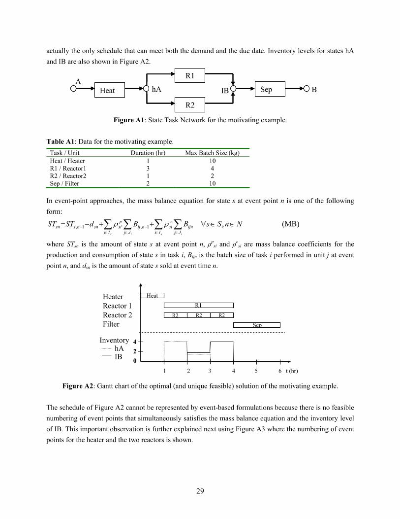
29

actually the only schedule that can meet both the demand and the due date. Inventory levels for states hA and IB are also shown in Figure A2.

BIBhAA

Heat

R1

R2

Sep BIBhAA

Heat

R1

R2

Sep

Figure A1: State Task Network for the motivating example.

Table A1: Data for the motivating example.

Task / Unit Duration (hr) Max Batch Size (kg) Heat / Heater 1 10 R1 / Reactor1 3 4 R2 / Reactor2 1 2 Sep / Filter 2 10

In event-point approaches, the mass balance equation for state s at event point n is one of the following form:

NnSsBBdSTSTisis Jj

ijnIi

csi

Jjnij

Ii

psisnnssn ∈∈∀++−= ∑∑∑∑

∈∈∈−

∈− ,1,1, ρρ (MB)

where STsn is the amount of state s at event point n, ρpsi and ρc

si are mass balance coefficients for the production and consumption of state s in task i, Bijn is the batch size of task i performed in unit j at event point n, and dsn is the amount of state s sold at event time n.

4

2

InventoryhAIB

HeaterReactor 1Reactor 2Filter

1 2 3 4 5 6 t (hr)

HeatR1

R2 R2 R2

Sep

420

Figure A2: Gantt chart of the optimal (and unique feasible) solution of the motivating example.

The schedule of Figure A2 cannot be represented by event-based formulations because there is no feasible numbering of event points that simultaneously satisfies the mass balance equation and the inventory level of IΒ. This important observation is further explained next using Figure A3 where the numbering of event points for the heater and the two reactors is shown.

30

Assume that the first event point for the heater is k. In order to satisfy equation (MB), the event points for Reactors 1 and 2 that start at t=1 must be numbered as n=k+1. Thus, neglecting dsn, the mass balance equation for state s=hA at time point n=k+1 reads: SThA,k+1 = SThA,k + Bht,H,,k – BRxn1,R1,k+1 – BRxn2,R2,k+1 ⇒ 4 = 0 + 10 – 4 – 2 which holds true. The event point for the second and the third batch of reaction 2 are naturally numbered as k+2 and k+3, respectively, and the corresponding mass balance equations for s=hA are: n=k+2: SThA,k+2 = SThA,k+1 – BRxn2,R2,k+2 ⇒ 2 = 4 – 2 n=k+3: SThA,k+3 = SThA,k+2 – BRxn2,R2,k+3 ⇒ 0 = 2 – 2 which also hold true. Given this numbering of Figure A3, there is no numbering for the event point of separation that simultaneously satisfies equation (MS) and the inventory levels of Figure A2. To prove this, let us first assume that the separation takes place at event point n=k+4. Then the mass balance for state IB at times t=2 and t=4 correspond to points n=k+2 and n=k+4, respectively, and read: n=k+2: STIB,k+2 = STIB,k+1 + BRxn1,R1,k+1 + BRxn2,R2,k+1 ⇒ 2 = 0 + 4 + 2 n=k+4: STIB,k+4 = STIB,k+3 + BRxn2,R2,k+3 – BSep,F,k+4 ⇒ 0 = 4 + 2 – 10 both of which are false.

1 2 3 4 5 6 t (hr)

Heater Reactor 1 Reactor 2 Filter

k

k+1

k+1 k+2 k+3

Figure A3: Numbering of event points of the motivating example.

Next, assume that the separation takes place at k+2 event point, whose start corresponds to time t=4 (although for Reactor2 the start of event k+2 corresponds to t=2), and that the start of k+1 event corresponds to t=1. The mass balance for state IB is: STIB,k+2 = STIB,k+1 + BRxn1,R1,k+1 + BRxn2,R2,k+1 – BSep,F,k+2 ⇒ 0 = 0 + 4 + 2 – 10 which is also false. Thus, from this example it is clear that there is no feasible event numbering that simultaneously satisfies mass balances and inventory levels of the optimal solution. To address this problem, Ierapetritou and Floudas (1998b) proposed a modification where the storage of a state is treated as an additional task, and storage tanks are treated as units. In addition, for every storage task and event time, three constraints need to be added in the formulation, of which two are big-M constraints. This modification introduces O(|S|*|N|) new binary variables, where |S| is the cardinality of states and |N| the cardinality of event points, and thus leads to models whose computational performance can be potentially expensive.

31

Another complication caused by the non-common time grid is the monitoring of utility usage level. Consider the case depicted in Figure 2, for example, where 10 kg/hr of steam are required by tasks T1, T2 and T3. If a common grid is used, the calculation of required steam is straightforward: 10 kg/hr are required during the 2nd time interval (t=1 → 2), 20 kg/hr are required during the 3rd interval (t=2 → 3), 30 kg/hr are required during the 4th interval (t=3 → 4), etc. If the event point representation is used, the kth period is different for each task: it corresponds to t=1 → 4 for T1, t=3 → 7 for T2 and t=2 → 6 for T3. This gives rise to two problems: (a) the start and finish of the kth period are not uniquely defined, and (b) the resource consumption during the kth period has many different values. Due to these difficulties resource constraints cannot be rigorously incorporated within the proposed event-driven models, as these have been presented Although it has never been shown how, utility constraints can potentially be addressed by event driven models by introducing a new state for each resource and expressing the corresponding mass balances and, more importantly, by increasing the number of events to overcome the two above mentioned difficulties. By increasing the number of events, however, the main advantage of event-driven models, namely the small number of events compared to models with common time partitioning, disappears.

Appendix B: Derivation of Mixed-Integer Constraints (C) and (12) Derivation of equation (C) For the derivation of equation (C), consider the two cases depicted in Figure B1, where we have assumed that k tasks have been assigned to unit j and start before time n. Obviously, k-1 of these tasks have finished before time n. If the (k-1)th task finishes at n*<n, then the following equation holds true:

0)1()1(*'

'*'

' =−−−=− ∑∑≤<

kkZfZsnn

jnnn

jn

In the case where no task is being processed in unit j at time n (Figure B1a), the kth task starts at or after n* and finishes at or before n:

011'*

''*

' =−=− ∑∑≤<<≤ nnn

jnnnn

jn ZfZs

and, thus, equation (C) holds true:

000'*

''*

'*'

'*'

''

''

' =+=

−+

−=−= ∑∑∑∑∑∑

≤<<≤≤<≤< nnnjn

nnnjn

nnjn

nnjn

nnjn

nnjnjn ZfZsZfZsZfZsZp

In the case where a task is being processed in unit j at time n (Figure B1b), the kth task starts at or after n*, but does not finish until n,

101'*

''*

' =−=− ∑∑≤<<≤ nnn

jnnnn

jn ZfZs

which makes equation (C) correct again,

32

110'*

''*

'*'

'*'

''

''

' =+=

−+

−=−= ∑∑∑∑∑∑

≤<<≤≤<≤< nnnjn

nnnjn

nnjn

nnjn

nnjn

nnjnjn ZfZsZfZsZfZsZp

1st 2nd (k-1)th kth

(a) Zpjn = 0

(b) Zpjn = 1

1st 2nd (k-1)th kth

n* n Figure B1: Alternative cases for binary Zpjn.

In a similar way, it can be shown that binary Wpin is calculated by the following equation:

njWfWsWpnn

jnnn

jnjn ∀∀−= ∑∑≤<

,'

''

' (C*)

Using (C*), binary Wpin can be eliminated in disjunction (F). Derivation of Assignment Constraint (12) Logical expressions (A) and (B) can be converted into integer equations (A*) and (B*) respectively:

njWsZsjIi

injn ∀∀= ∑∈

,)(

(A*)

njWfZfjIi

injn ∀∀= ∑∈

,)(

(B*)

Replacing the implication (D) by its equivalent disjunction, and using the definitions of binaries Zsjn, Zpjn and Zfjn [equations (A*), (B*) and (C)], we get constraint (12) which is the basic assignment constraint:

( )⇔¬⇒ jnjn ZpZs

( )⇔¬∨¬ jnjn ZpZs

( ) ( )( )⇔≥−+− 111 jnjn ZpZs

( ) ⇔

≥

−−+− ∑∑

≤<

111'

''

'nn

jnnn

jnjn ZfZsZs

⇔

≥+− ∑∑

≤≤

12'

''

'nn

jnnn

jn ZfZs

( ) ⇔

≤−∑

≤nnjnjn ZfZs

''' 1

33

⇔≤

−∑ ∑∑

≤ ∈∈nn jIiin

jIiin WfWs

' )('

)(' 1

njWfWsjIi nn

inin ∀∀≤−∑ ∑∈ ≤

,1)()( '

'' (12)

Appendix C: Data for Examples Table C1: Data for Example 1.

A B C HotA IntAB IntBC ImE P1 P2 Cs (kg) 1,000 1,000 1,000 100 200 150 200 1,000 1,000 S0s (kg) 1,000 1,000 1,000 0 0 0 0 0 0 gs ($/kg) 0 0 0 0 0 0 0 10 10

Table C2: Data for Example 1 (constant processing times).

Task Duration (hr) ΒΜΑΧ

Heater Reactor I Reactor II Column Heating 1 100 - - - Reaction 1 2 - 50 80 - Reaction 2 2 - 50 80 - Reaction 3 1 - 50 80 - Separation 2 - - - 200

Table C3: Data for Example 1 (variable processing times).

Task BMAX Heating Reaction 1 Reaction 2 Reaction 3 Separation α β α β α β α β α β Heater 100 .667 .00667 - - - - - - - - Reactor I 50 - - 1.334 .02664 1.334 .02664 .667 .01332 - - Reactor II 80 - - 1.334 .01665 1.334 .01665 .667 .008325 - - Column 200 - - - - - - - - 1.3342 .00666

Table C4: Data for Example 2.

R1 R2 I1 I2 I3 P1 P2 Cs (kg) 1,000 1,000 200 100 500 1,000 1,000 S0s (kg) 400 400 0 0 0 0 0 gs ($/kg) 10 15 25 0 0 30 40

Table C5: Data for Example 2 (BMIN / BMAX in kg, α in hr, β in hr/kg).

Task BMIN BMAX R1 R2 R3 R4 Min/Mean/Max d 1.5/2.0/2.5 2.25/3.0/3.75 0.75/1.0/1.25 1.5/2.0/2.5 α β α β α β α β RI1 40 80 0.5 0.025 0.75 0.0375 - - - - RI2 25 50 0.5 0.04 0.75 0.06 - - - - RII 80 80 - - - - 0.25 0.0125 0.5 0.025

34

Table C6: Resource requirements for Example 2 (γ in kg/min, δ in kg/min per kg of batch). R1 R2 R3 R4 γiHS δhis γiCW δiCW γiHS δiHS γiCW δiCW RI1 6 0.25 4 0.3 - - - - RI2 4 0.25 3 0.3 - - - - RII - - - - 8 0.2 4 0.5

Table C7: Data for Example 3.

F1 F2 S1 S2 S3 S4 S5 S6 INT1 INT2 P1 P2 P3 Cs (kg) ∞ ∞ 0 0 15 40 0 0 ∞ ∞ ∞ ∞ ∞ S0s (kg) 100 100 0 0 0 10 0 0 0 0 0 0 0 gs (103$/kg) - - - - - - - - - - 1 1 1

Table C8: Data for Example 3 (BMAX in kg, α in hr, γ in kg/min, δ in kg/min per kg of batch).

Task T1 T2 T3 T4 T5 T6 T7 T8 T9 T10 Unit U1 U2 U3 U1 U4 U4 U5 U6 U5 U6 BMAX 5 8 6 5 8 8 3 4 3 4 α 2 1 1 2 2 2 4 2 2 3 Utility LPS CW LPS HPS LPS HPS CW LPS CW CW γ 3 4 4 3 8 4 5 5 5 3 δ 2 2 3 2 4 3 4 3 3 3

Table C9: Data for Example 4.

F1 F2 S11 S12 S12 S22 P1 P2 Cs (kg) 100 100 5 in T1 5 in T1 3 in T2 3 in T2 100 100 S0s (kg) 100 100 0 0 0 0 0 0 gs (103$/kg) - - - - - - 1 1

Table C10: Data for Example 4 (BMAX, BMIN in tons, α in hr, β in hr/ton of batch).

Task T11 T21 T12 T22 T13 T23 Unit U1 U1 U2 U2 U3 U3 BMAX 5 5 3 3 3 3 BMIN 2 2 1.2 1.2 1.2 1.2 α 1 0.5 0.5 0.75 0.75 0.5 β 0.8 0.667 0.667 0.6

Table C11: Setup times for Example 4 (hr)

T11 T21 T12 T22 T13 T23 T11 0 0.2 0.1 0.5 T21 0.3 0 0.6 0.4 T12 0 0.3 T22 0.2 0 T13 0.2 0.6 0 0.5 T23 0.5 0.3 0.4 0

35

References (1) Kondili, E.; Pantelides, C. C.; Sargent, R. A General Algorithm for Short-Term Scheduling of Batch

Operations – I. MILP Formulation. Comput. Chem. Eng. 1993, 17, 211-227. (2) Shah, N.; E.; Pantelides, C. C.; Sargent, R. A General Algorithm for Short-Term Scheduling of Batch

Operations – IΙ. Computational Issues. Comput. Chem. Eng. 1993, 17, 229-244. (3) Pantelides, C. C. Unified Frameworks for the Optimal Process Planning and Scheduling. Proceedings

on the Second Conference on Foundations of Computer Aided Operations. 1994, 253-274. (4) Schilling, G.; Pantelides, C. C. A Simple Continuous-Time Process Scheduling Formulation and a

Novel Solution Algorithm. Comput. Chem. Eng. 1996, 20, S1221-1226. (5) Zhang, X.; Sargent, R. W. H. The Optimal Operation of Mixed Production Facilities – General

Formulation and Some Approaches for the Solution. Comput. Chem. Eng. 1996, 20, 897-904. (6) Mockus, L.; Reklaitis, G.V. Continuous Time Representation Approach to Batch and Continuous

Process Scheduling. 1. MINLP Formulation. Ind. Eng. Chem. Res. 1999, 38, 197-203. (7) Castro, P.; Barbosa-Povoa, A. P. F. D.; Matos, H. An Improved RTN Continuous-Time Formulation

for the Short-term Scheduling of Multipurpose Batch Plants. Ind. Eng. Chem. Res. 2001, 40, 2059-2068.

(8) Ierapetritou, M. G.; Floudas, C. A. Effective Continuous-Time Formulation for Short-Term Scheduling. 1. Multipurpose Batch Processes. Ind. Eng. Chem. Res. 1998, 37, 4341-4359.

(9) Rodrigues, M.T.; Luis G. Latre, Luis Carlos A. Rodrigues. Short-Term Planning and Scheduling in Multipurpose Batch Chemical Plants: a Multilevel Approach. Comp. Chem. Eng. 2000, 24, 2247-2258.

(10) Mendez, C.A.; Henning, G.P.; Cerda, J. Optimal Scheduling of Batch Plants Satisfying Multiple Product Orders with Different Due-Dates. Comp. Chem. Eng. 2000, 24, 2223-2245.

(11) Lee, K.; Il Park, H.; In Beum Lee. A Novel Nonuniform Discrete Time Formulation for Short-Term Scheduling of Batch and Continuous Processes. Ind. Eng. Chem. Res. 2001, 40, 4902-4911.

(12) Giannelos, N.F.; Georgiadis, M.C. A Simple New Continuous-Time Formulation for Short-Term Scheduling of Multipurpose Batch Processes. Ind. Eng. Chem. Res. 2002, 41, 2178-2184.

(13) Raman, R.; Grossmann, I.E. Modeling and Computational Techniques for Logic-Based Integer Programming. Comput. Chem, Eng. 1994, 18, 563-578

(14) Vecchietti, A.; Grossmann, I.E. LOGMIP: A Disjunctive 0-1 Non-Linear Optimizer for Process System Models. Comput. Chem. Eng. 1999, 23 (4-5), 555-556.

(15) Balas, E. Disjunctive Programming and Hierarchy of Relaxations for Discrete Optimization Problems. SIAM J. Alg. Disc. Math. 1985, 35, 2611-2623.

(16) Raman, R.; Grossmann, I.E. Relation between MILP Modeling and Logical Inference for Chemical Process Synthesis. Comput. Chem. Eng., 1991, 15 (2), 73-84.

(17) Maravelias, C.T.; Grossmann, I.E. A Hybrid MILP/CP Decomposition Approach for the Short Term Scheduling of Multipurpose Batch Plants. Manuscript under preparation.

(18) Maravelias, C.T.; Grossmann, I.E. A New Continuous-Time State Task Network Formulation for Short Term Scheduling of Multipurpose Batch Plants with Due Dates. Accepted for presentation in PSE 2003, Kunming, China.

(19) Papageorgiou, L.G.; Pantelides, C.C. Optimal Campaign Planning/Scheduling of Multipurpose Batch/Semicontinuous Plants. 2. Mathematical Decomposition Approach. Ind. Eng. Chem. Res. 1996, 35, 510-529.

(20) Ierapetritou, M.G.; Floudas, C.A. Comments on “An Improved RTN Continuous-Time Formulation for the Short-term Scheduling of Multipurpose Batch Plants”. Ind. Eng. Chem. Res. 2001, 40, 5040-5041.

(21) Ierapetritou, M. G.; Floudas, C. A. Effective Continuous-Time Formulation for Short-Term Scheduling. 2. Continuous and Semicontinuous Processes. Ind. Eng. Chem. Res. 1998, 37, 4360-4374.

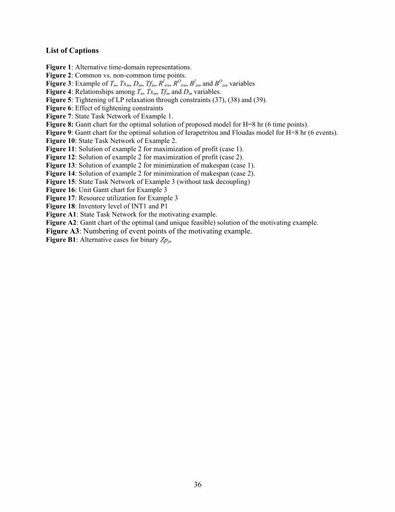
36

List of Captions Figure 1: Alternative time-domain representations. Figure 2: Common vs. non-common time points. Figure 3: Example of Tn, Tsin, Din, Tfin, RI

irn, ROirn, BI

isn and BOisn variables

Figure 4: Relationships among Tn, Tsin, Tfin and Din variables. Figure 5: Tightening of LP relaxation through constraints (37), (38) and (39). Figure 6: Effect of tightening constraints Figure 7: State Task Network of Example 1. Figure 8: Gantt chart for the optimal solution of proposed model for H=8 hr (6 time points). Figure 9: Gantt chart for the optimal solution of Ierapetritou and Floudas model for H=8 hr (6 events). Figure 10: State Task Network of Example 2. Figure 11: Solution of example 2 for maximization of profit (case 1). Figure 12: Solution of example 2 for maximization of profit (case 2). Figure 13: Solution of example 2 for minimization of makespan (case 1). Figure 14: Solution of example 2 for minimization of makespan (case 2). Figure 15: State Task Network of Example 3 (without task decoupling) Figure 16: Unit Gantt chart for Example 3 Figure 17: Resource utilization for Example 3 Figure 18: Inventory level of INT1 and P1 Figure A1: State Task Network for the motivating example. Figure A2: Gantt chart of the optimal (and unique feasible) solution of the motivating example. Figure A3: Numbering of event points of the motivating example. Figure B1: Alternative cases for binary Zpjn

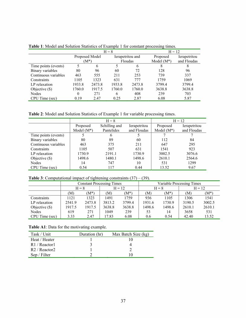
37

Table 1: Model and Solution Statistics of Example 1 for constant processing times.

H = 8 H = 12 Proposed Model

(M*) Ierapetritou and

Floudas Proposed

Model (M*) Ierapetritou and Floudas

Time points (events) 5 6 5 6 8 8 Binary variables 80 96 60 72 128 96 Continuous variables 463 555 211 253 739 337 Constraints 1105 1323 631 777 1759 1069 LP relaxation 1933.8 2473.8 1933.8 2473.8 3799.4 3799.4 Objective ($) 1760.0 1917.5 1760.0 1760.0 3638.8 3638.8 Nodes 0 271 6 408 239 703 CPU Time (sec) 0.19 2.47 0.25 2.87 6.08 5.87

Table 2: Model and Solution Statistics of Example 1 for variable processing times.

H = 8 H = 12 Proposed

Model (M*) Schilling and

Pantelides Ierapetritou and Floudas

Proposed Model (M*)

Ierapetritou and Floudas

Time points (events) 5 6 5 7 7 Binary variables 80 89 60 112 84 Continuous variables 463 375 211 647 295 Constraints 1105 507 631 1541 923 LP relaxation 1730.9 2191.1 1730.9 3002.5 3076.6 Objective ($) 1498.6 1480.1 1498.6 2610.1 2564.6 Nodes 14 747 10 531 1299 CPU Time (sec) 0.54 117 0.44 13.52 9.67

Table 3: Computational impact of tightening constraints (37) – (39).

Constant Processing Times Variable Processing Times H = 8 H = 12 H = 8 H = 12 (M) (M*) (M) (M*) (M) (M*) (M) (M*) Constraints 1121 1323 1491 1759 936 1105 1306 1541 LP relaxation 2541.9 2473.8 3813.2 3799.4 1931.6 1730.9 3190.5 3002.5 Objective ($) 1917.5 1917.5 3638.8 3638.8 1498.6 1498.6 2610.1 2610.1 Nodes 619 271 1049 239 53 14 3658 531 CPU Time (sec) 3.33 2.47 17.83 6.08 0.6 0.54 42.40 13.52

Table A1: Data for the motivating example. Task / Unit Duration (hr) Max Batch Size (kg) Heat / Heater 1 10 R1 / Reactor1 3 4 R2 / Reactor2 1 2 Sep / Filter 2 10

38

i Papageorgiou, L.G.; Pantelides, C.C. Optimal Campaign Planning/Scheduling of Multipurpose

Batch/Semicontinuous Plants. 2. Mathematical Decomposition Approach. Ind. Eng. Chem. Res. 1996, 35, 510-529.

ii Ierapetritou, M.G.; Floudas, C.A. Comments on “An Improved RTN Continuous-Time Formulation for the Short-term Scheduling of Multipurpose Batch Plants”. Ind. Eng. Chem. Res. 2001, 40, 5040-5041.