arX

iv:1

602.

0226

9v3

[m

ath.

FA]

25

Jun

2017

A new inequality for the Riemann-Stieltjes integrals

driven by irregular signals in Banach spaces

Rafał M. Łochowski

10th August 2018

Abstract

We prove an inequality of the Loéve-Young type for the Riemann-Stieltjes integralsdriven by irregular signals attaining their values in Banach spaces and, as a result, wederive a new theorem on the existence of the Riemann-Stieltjes integrals driven by suchsignals. Also, for any p ≥ 1 we introduce the space of regulated signals f : [a, b] → W(a < b are real numbers and W is a Banach space), which may be uniformly approximatedwith accuracy δ > 0 by signals whose total variation is of order δ1−p as δ → 0+ and provethat they satisfy the assumptions of the theorem. Finally, we derive more exact, rate-independent characterisations of the irregularity of the integrals driven by such signals.

Keywords: regulated path, total variation, p-variation, truncated variation, the Riemann-Stieltjes integral, the Loéve-Young inequality, Banach space.Mathematics Subject Classification (2010): 46B99, 46G10.

1 Introduction

The first aim of this paper is a generalisation of the results of [6] and [5] to the functionsattaining their values not only in R but in more general spaces. Next, to obtain moreprecise results, for any p ≥ 1 we introduce the space Up ([a, b] ,W ) of regulated func-tions/signals f : [a, b] → W (a < b are real numbers and W is a Banach space), whichmay be uniformly approximated with accuracy δ > 0 by functions whose total variationis of order δ1−p as δ → 0 + . This way we will obtain a result about the existence of theRiemann-Stieltjes integral

´ ba fdg for functions from Up ([a, b]) and Uq ([a, b]) whenever

p, q > 1, p−1 + q−1 > 1. Results of this type were earlier obtained by Young [12], [13] andD’yačkov [4] (for very detailed account see [3, Chapt. 3]) but they were expressed in termsof p- or (more general) φ-variations.

In [6] the following variational problem was considered: given real a < b, c > 0, aregulated function/signal f : [a, b] → R (for the definition of a regulated function see thenext section) and x ∈ [f (a)− c/2, f (a) + c/2] , find the infimum of total variations of allfunctions f c,x : [a, b] → R which uniformly approximate f with accuracy c/2,

‖f − f c,x‖[a,b],∞ := supa≤t≤b

|f (t)− f c,x (t)| ≤ c/2,

and start from x, f c,x (a) = x. Recall that for g : [a, b] → R its total variation is defined as

TV(g, [a, b]) := supn

supa≤t0<t1<...<tn≤b

n∑

i=1

|g (ti)− g (ti−1)| .

1

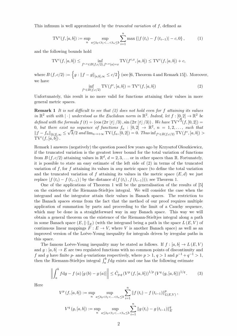
This infimum is well approximated by the truncated variation of f, defined as

TVc(f, [a, b]) := supn

supa≤t0<t1<...<tn≤b

n∑

i=1

max {|f (ti)− f (ti−1)| − c, 0} , (1)

and the following bounds hold

TVc(f, [a, b]) ≤ inffc,x∈B(f,c/2),fc,x(a)=x

TV(f c,x, [a, b]) ≤ TVc(f, [a, b]) + c,

where B (f, c/2) :={

g : ‖f − g‖[a,b],∞ ≤ c/2}

(see [6, Theorem 4 and Remark 15]). Moreover,

we haveinf

fc∈B(f,c/2)TV(f c, [a, b]) = TVc(f, [a, b]) (2)

Unfortunately, this result is no more valid for functions attaining their values in moregeneral metric spaces.

Remark 1 It is not difficult to see that (2) does not hold even for f attaining its valuesin R

2 with with | · | understood as the Euclidean norm in R2. Indeed, let f : [0, 2] → R

2 be

defined with the formula f (t) = (cos (2π ⌊t⌋ /3) , sin (2π ⌊t⌋ /3)) . We have TV√3(f, [0, 2]) =

0, but there exist no sequence of functions fn : [0, 2] → R2, n = 1, 2, . . . , such that

‖f − fn‖[0,2],∞ ≤√3/2 and limn→+∞ TV(fn, [0, 2]) = 0. Thus inffc∈B(f,c/2) TV(f c, [a, b]) >

TVc(f, [a, b]) .

Remark 1 answers (negatively) the question posed few years ago by Krzysztof Oleszkiewicz,if the truncated variation is the greatest lower bound for the total variation of functionsfrom B (f, c/2) attaining values in R

d, d = 2, 3, . . . or in other spaces than R. Fortunately,it is possible to state an easy estimate of the left side of (2) in terms of the truncatedvariation of f, for f attaining its values in any metric space (to define the total variationand the truncated variation of f attaining its values in the metric space (E, d) we justreplace |f (ti)− f (ti−1) | by the distance d (f (ti) , f (ti−1))); see Theorem 1.

One of the applications of Theorem 1 will be the generalisation of the results of [5]on the existence of the Riemann-Stieltjes integral. We will consider the case when theintegrand and the integrator attain their values in Banach spaces. The restriction tothe Banach spaces stems from the fact that the method of our proof requires multipleapplication of summation by parts and proceeding to the limit of a Cauchy sequence,which may be done in a straightforward way in any Banach space. This way we willobtain a general theorem on the existence of the Riemann-Stieltjes integral along a pathin some Banach space (E, ‖·‖E) (with the integrand being a path in the space L (E,V ) ofcontinuous linear mappings F : E → V, where V is another Banach space) as well as animproved version of the Loéve-Young inequality for integrals driven by irregular paths inthis space.

The famous Loéve-Young inequality may be stated as follows. If f : [a, b] → L (E,V )and g : [a, b] → E are two regulated functions with no common points of discontinuity andf and g have finite p- and q-variations respectively, where p > 1, q > 1 and p−1+ q−1 > 1,then the Riemann-Stieltjes integral

´ ba fdg exists and one has the following estimate

∥

∥

∥

∥

ˆ b

afdg − f (a) [g (b)− g (a)]

∥

∥

∥

∥

≤ C̃p,q (Vp (f, [a, b]))1/p (V q (g, [a, b]))1/q . (3)

Here

V p (f, [a, b]) := supn

supa≤t0<t1<...<tn≤b

n∑

i=1

‖f (ti)− f (ti−1)‖pL(E,V ) ,

V q (g, [a, b]) := supn

supa≤t0<t1<...<tn≤b

n∑

i=1

‖g (ti)− g (ti−1)‖qE

2

denote p- and q-variation of f and g respectively (sometimes called the strong variation).The original Loéve-Young estimate, with the constant C̃p,q = 1 + ζ (1/p + 1/q) , whereζ is the famous Riemann zeta function, was formulated for real functions in [12]. Thecounterpart of this inequality for more general, Banach space-valued functions, with theconstant C̃p,q = 41/p+1/qζ (1/p + 1/q) , is formulated in the proof of [9, Theorem 1.16].Our, improved version of (3) is the following

∥

∥

∥

∥

ˆ b

afdg − f (a) [g (b)− g (a)]

∥

∥

∥

∥

≤ Cp,q (Vp (f, [a, b]))1−1/q ‖f‖1+p/q−p

osc,[a,b] (V q (g, [a, b]))1/q ,

where ‖f‖osc,[a,b] := supa≤s<t≤b ‖f (s)− f (t)‖L(E,V ) and Cp,q is a universal constant de-

pending on p and q only. Notice that always

(V p (f, [a, b]))1/p−(1−1/q) ≥ ‖f‖1+p/q−posc,[a,b] .

These results may be applied for example when f and g are trajectories of α-stableprocesses X1, X2 with α ∈ (1, 2). However, since the obtained results are formulated interms of rate-independent functionals, like the truncated variation or p-variation, theyremain valid when f (t) = F

(

X1 (A (t)))

and g (t) = G(

X2 (B (t)))

(with the technicalassumption that the jumps of f and g do not occur at the same time) where A,B :[0,+∞) → [0,+∞) are piecewise monotonic, possibly random, changes of time (i.e. thereexist 0 = T0 < T1 < . . . such that Tn → +∞ almost surely as n → +∞ and A and Bare monotonic on each interval (Ti−1, Ti) , i = 1, 2, . . .), while F,G : R → R are locallyLipschitz.

It appears that it is possible to derive weaker conditions under which the improvedLoéve-Young inequality still holds, and we will prove that it still holds (and the Riemann-

Stieltjes integral´ ba fdg exists) for functions f and g with no commont poins of discon-

tinuity, satisfying

supδ>0

δp−1TVδ(f, [a, b]) < ∞ and supδ>0

δq−1TVδ(g, [a, b]) < ∞

respectively. Moreover, in such a case the indefinite integral I (t) :=´ ta fdg reveals similar

irregularity as the integrator g, namely, supδ>0 δq−1TVδ(I, [a, b]) < ∞. We will also prove

that for any p ≥ 1 the class of functions f : [a, b] → W, where W is some Banach space,such that TVδ(f, [a, b]) = O

(

δ1−p)

as δ → 0+, is a Banach space. We will denote it byUp ([a, b],W ) . The property f ∈ Up ([a, b],W ) is weaker than the existence of p-variationbut stronger than the existence of q-variation for some q > p.

From early work of Lyons [8] it is well known that whenever f and g have finite p- andq-variations respectively, p > 1, q > 1 and p−1 + q−1 > 1, then the indefinite integral I(·)has finite q-variation. However, it is also well known that a symmetric α-stable process Xwith α ∈ [1, 2] has finite p-variation for any p > α while its α-variation is infinite (on anyproper, compact subinterval of [0,+∞)), see for example [1, Theorem 4.1]. Thus, if forexample f (t) = F

(

X1 (A (t)))

and g (t) = G(

X2 (B (t)))

are like in a former paragraph,we can say that I (·) has finite p-variation, on any compact subinterval of [0,+∞) for anyp > α, but can not say much more. From our results it will follow that I (·) ∈ Uα ([0, t],R)for any t ≥ 0. As far as we know, no such result is known in the case when the integratorhas finite φ-variation except the already mentioned case φ(x) = |x|q.

Let us comment on the organization of the paper. In the next section we prove verygeneral estimates for infg∈B(f,c/2) TV(g, [a, b]) , for regulated f : [a, b] → E, where E isany metric space, in terms of the truncated variation of f. Next, in the third section, weuse obtained estimates to prove a new theorem on the existence of the Riemann-Stieltjesintegral driven by irregular paths in Banach spaces. In the proofs we follow closely [5]. Inthe last, fourth section we introduce the Banach spaces Up ([a, b],W ) , p ≥ 1, (subsection

3

4.1) and in subsection 4.2 obtain more exact estimates of the rate-independent irregularityof functions from these spaces (in terms of φ−variation). In the last subsection we dealwith the irregularity of the integrals driven by signals from the spaces Up ([a, b],W ) , p ≥ 1.

2 Estimates for the variational problem

Let (E, d) be a metric space with the metric d. For given reals a < b we say that thefunction f : [a, b] → E is regulated if it has right limits f (t+) for any t ∈ [a, b) and leftlimits f (t−) for any t ∈ (a, b] . If E is complete then a necessary and sufficient conditionfor f to be regulated is that it is an uniform limit of step functions (see [2, Theorem 7.6.1]).

Let f : [a, b] → E be regulated. For c > 0 let us consider the family B (f, c/2) of allfunctions g : [a, b] → E such that supt∈[a,b] d (f (t) , g (t)) ≤ c/2. We will be interested inthe followng variational problem: find

infg∈B(f,c/2)

TV(g, [a, b]) , (4)

where

TV(g, [a, b]) := supn

supa≤t0<t1<...<tn≤b

n∑

i=1

d (g (ti) , g (ti−1)) .

To state our first main result let us define

TVc(g, [a, b]) := supn

supa≤t0<t1<...<tn≤b

n∑

i=1

max {d (g (ti) , g (ti−1))− c, 0} .

Theorem 1 For any regulated f : [a, b] → E there exists a step function f c : [a, b] →E such that supt∈[a,b] d (f (t) , f c (t)) ≤ c/2 and for any λ > 1, TV(f c, [a, b]) ≤ λ ·TV(λ−1)c/(2λ)(f, [a, b]) . Thus the following estimates hold

TVc(f, [a, b]) ≤ infg∈B(f,c/2)

TV(g, [a, b]) ≤ infλ>1

λ · TV(λ−1)c/(2λ)(f, [a, b]) .

In particular, taking λ = 2 we get the double-sided estimate

TVc(f, [a, b]) ≤ infg∈B(f,c/2)

TV(g, [a, b]) ≤ 2 · TVc/4(f, [a, b]) .

Moreover, if E is a vector normed space with the norm ‖·‖E then there exists f c,lin :[a, b] → E such that f c,lin is piecewise linear, jumps of f c,lin occur only at the pointswhere the jumps of f occur, supt∈[a,b]

∥

∥f (t)− f c,lin (t)∥

∥

E≤ c and TV

(

f c,lin, [a, b])

=TV(f c, [a, b]) .

Proof. The estimate from below

infg∈B(f,c/2)

TV(g, [a, b]) ≥ TVc(f, [a, b])

follows immediately from the triangle inequality: if supt∈[a,b] d (f (t) , g (t)) ≤ c/2 then forany a ≤ s < t ≤ b,

max {d (g (t) , g (s))− c, 0} ≤ max {d (g (t) , g (s))− d (g (t) , f (t))− d (g (s) , f (s)) , 0}≤ d (f (t) , f (s)) .

The estimate from above follows from the following greedy algorithm. Let us considerthe sequence of times defined in the following way: τ0 = a and for n = 1, 2, . . .

τn =

inf {t ∈ (τn−1, b] : d (f (t) , f (τn−1)) > c/2}if τn−1 < b and d (f (τn−1) , f (τn−1+)) < c/2;

inf {t ∈ (τn−1, b] : d (f (t) , f (τn−1+)) > c/2}if τn−1 < b and d (f (τn−1) , f (τn−1+)) ≥ c/2;

+∞ otherwise.

4

Note that, since f is regulated, limn→+∞ τn = +∞. (We apply the convention that inf ∅ =+∞.) Now we define a step function f c ∈ B (f, c/2) in the following way. For eachn = 1, 2, . . . such that τn−1 < b we put

• if d (f (τn−1) , f (τn−1+)) < c/2 then

f c (t) := f (τn−1) for t ∈ [τn−1, τn) ∩ [a, b] ;

• if d (f (τn−1) , f (τn−1+)) ≥ c/2 then f c (τn−1) := f (τn−1) and

f c (t) := f (τn−1+) for t ∈ (τn−1, τn) ∩ [a, b] .

This way the function f c is defined for all t ∈ [a, b].It is not difficult to see that the just constructed f c satisfies supt∈[a,b] d (f (t) , f c (t)) ≤

c/2 and for each n = 1, 2, . . . such that τn ≤ b we have

• if d (f (τn−1) , f (τn−1+)) < c/2 then

d (f c (τn−1) , fc (τn−1+)) = 0 (5)

and

d (f c (τn−1+) , f c (τn)) = d (f (τn−1) , f (τn)) ≥ c/2; (6)

• if d (f (τn−1) , f (τn−1+)) ≥ c/2 then

d (f c (τn−1) , fc (τn−1+)) = d (f (τn−1+) , f (τn−1+)) ≥ c/2 (7)

andd (f c (τn−1+) , f c (τn)) = d (f (τn−1+) , f (τn)) ≥ c/2. (8)

Let N = max {n : τn−1 < b} . From an elementary inequality x ≤ λmax{

x− λ−12λ c, 0

}

valid for any x ∈ {0} ∪ [c/2,+∞) and λ > 1, and (5) - (8) we have

TV(f c, [a, b]) =

N∑

n=1

{d (f c (τn−1) , fc (τn−1+)) + d (f c (τn−1+) , f c (τn ∧ b))}

≤ λ

N∑

n=1

max

{

d (f c (τn−1) , fc (τn−1+))− λ− 1

2λc, 0

}

+ λN∑

n=1

max

{

d (f c (τn−1) , fc (τn ∧ b))− λ− 1

2λc, 0

}

≤ λ

N∑

n=1

max

{

d (f (τn−1) , f (τn−1+))− λ− 1

2λc, 0

}

+ λ

N∑

n=1

max

{

d (f (τn−1+) , f (τn ∧ b))− λ− 1

2λc, 0

}

≤ λTV(λ−1)c/(2λ)(f, [a, b]) .

Thus, since f c ∈ B (f, c/2) and λ was an arbitrary number from the interval (1,+∞) , wehave

infg∈B(f,c/2)

TV(g, [a, b]) ≤ TV(f c, [a, b]) ≤ infλ>1

λ · TV(λ−1)c/(2λ)(f, [a, b]) .

The construction of the function f c,lin is similar. For τn, n = 0, 1, . . . , such that τn ≤ b,we define f c,lin (τn) = f (τn) and for t ∈ (τn−1, τn) ∩ [a, b], n = 0, 1, . . . such that τn−1 < bit is defined in the following way.

5

• If d (f (τn−1) , f (τn−1+)) < c/2, τn ≤ b and f (τn−) 6= f (τn) then for t ∈ (τn−1, τn)we put

f c,lin (t) := f (τn−1) ;

• if d (f (τn−1) , f (τn−1+)) < c/2 and τn = +∞ then for t ∈ (τn−1, b] we put

f c,lin (t) := f (τn−1) ;

• if d (f (τn−1) , f (τn−1+)) < c/2, τn ≤ b and f (τn−) = f (τn) then for t ∈ (τn−1, τn)we put

f c,lin (t) :=τn − t

τn − τn−1f (τn−1) +

t− τn−1

τn − τn−1f (τn) ;

• if d (f (τn−1) , f (τn−1+)) ≥ c/2, τn ≤ b and f (τn−) 6= f (τn) then for t ∈ (τn−1, τn)we put

f c,lin (t) := f (τn−1+) ;

• if d (f (τn−1) , f (τn−1+)) ≥ c/2 and τn = +∞ then for t ∈ (τn−1, b] we put

f c,lin (t) := f (τn−1+) ;

• if d (f (τn−1) , f (τn−1+)) ≥ c/2, τn ≤ b and f (τn−) = f (τn) then for t ∈ (τn−1, τn)

f c,lin (t) :=τn − t

τn − τn−1f (τn−1+) +

t− τn−1

τn − τn−1f (τn) .

It is straightforward to verify that supt∈[a,b]∥

∥f (t)− f c,lin (t)∥

∥

E≤ c, TV

(

f c,lin, [a, b])

=

TV(f c, [a, b]) and the jumps of f c,lin occur only at the points where the jumps of f occur.�

3 Integration of irregular signals in Banach spaces

Directly from the definition it follows that the truncated variation is a superadditive func-tional of the interval, i.e. for c ≥ 0 and any d ∈ (a, b)

TVδ(f, [a, b]) ≥ TVδ(f, [a; d]) + TVδ(f, [d, b]) . (9)

Moreover, if (E, ‖·‖E) is a normed vector space (with the norm ‖·‖E) we also have thefollowing easy estimate of the truncated variation of a function g : [a, b] → E perturbedby some other function h : [a, b] → E :

TVδ(g + h, [a, b]) ≤ TVδ(g, [a, b]) + TV0(h, [a, b]) , (10)

which stems directly from the inequality: for a ≤ s < t ≤ b,

max {‖g (t) + h (t)− {g (s) + h (s)}‖E − δ, 0}≤ max {‖g (t)− g (s)‖E − δ, 0} + ‖h (t)− h (s)‖E .

Let now (E, ‖·‖E) , (W, ‖·‖W ) be Banach spaces, (V, ‖·‖V ) be another Banach space

and(

L (E,V ) , ‖·‖L(E,V )

)

be the space of continuous linear mappings F : E → V with

the norm ‖F‖L(E,V ) = supe∈E:‖e‖E=1 ‖F · e‖V . Throughout the rest of this paper we willassume that f : [a, b] → W and g : [a, b] → E. We will often encounter the situation whenW = L (E,V ) .

Relations (9) and (10), together with Theorem 1, will allow us to establish the followingresult.

6

Theorem 2 Let f : [a, b] → L (E,V ) and g : [a, b] → E be two regulated functionswhich have no common points of discontinuity. Let η0 ≥ η1 ≥ . . . and θ0 ≥ θ1 ≥ . . .be two sequences of positive numbers, such that ηk ↓ 0, θk ↓ 0 as k → +∞. Defineη−1 :=

12 supa≤t≤b ‖f (t)− f (a)‖L(E,V ) and

S := 4

+∞∑

k=0

3kηk−1 · TVθk/4(g, [a, b]) + 4

∞∑

k=0

3kθk · TVηk/4(f, [a, b]) .

If S < +∞ then the Rieman-Stieltjes integral´ ba fdg exists and one has the following

estimate∥

∥

∥

∥

ˆ b

afdg − f (a) [g (b)− g (a)]

∥

∥

∥

∥

V

≤ S. (11)

Remark 2 For ξ, s, t ∈ [a, b] by f (ξ) [g (t)− g (s)] we mean the value of the linear map-ping f (ξ) evaluated at the vector g (t) − g (s) (i.e. the element of the space V ) and the

Riemann-Stieltjes integral´ ba fdg is understood as the limit (if it exists) of the sums

n∑

i=1

f(

ξ(n)i

) [

g(

t(n)i

)

− g(

t(n)i−1

)]

,

where for n = 1, 2, . . . , i = 1, 2, . . . , n, a = t(n)0 < t

(n)1 < . . . < t

(n)n = b, ξ

(n)i ∈

[

t(n)i−1, t

(n)i

]

and limn→+∞max1≤i≤n

(

t(n)i − t

(n)i−1

)

= 0.

The proof of Theorem 2 will be based on the following lemmas.

Lemma 1 (summation by parts in a Banach space) Let f : [a, b] → L (E,V ) , g :[a, b] → E and c = t0 < t1 < . . . < tn = d be any partition of the interval [c, d] ⊂ [a, b]. Letξ0 = c and ξ1, . . . , ξn be such that ti−1 ≤ ξi ≤ ti for i = 1, 2, . . . , n, then

n∑

i=1

[f (ξi)− f (c)] [g (ti)− g (ti−1)] =n∑

i=1

[f (ξi)− f (ξi−1)] [g (d)− g (ti−1)] . (12)

Proof. For i = 1, 2 . . . , n let us denote fi = f (ξi) − f (ξi−1) , gi = g (ti) − g (ti−1) . Wehave

n∑

i=1

[f (ξi)− f (c)] [g (ti)− g (ti−1)] =

n∑

i=1

i∑

j=1

fj

gi

=n∑

j=1

fj

n∑

i=j

gi

=n∑

i=1

[f (ξi)− f (ξi−1)] [g (d)− g (ti−1)] .

�

Lemma 2 Let f : [a, b] → L (E,V ) and g : [a, b] → E be two regulated functions. Letc = t0 < t1 < . . . < tn = d be any partition of the interval [c, d] ⊂ [a, b] and letξ0 = c and ξ1, . . . , ξn be such that ti−1 ≤ ξi ≤ ti for i = 1, 2, . . . , n. Then for δ−1 :=12 supc≤t≤d ‖f (t)− f (c)‖L(E,V ) and any δ0 ≥ δ1 ≥ . . . ≥ δr > 0 and ε0 ≥ ε1 ≥ . . . ≥ εr > 0the following estimate holds

∥

∥

∥

∥

∥

n∑

i=1

f (ξi) [g (ti)− g (ti−1)]− f (c) [g (d)− g (c)]

∥

∥

∥

∥

∥

V

≤ 4

r∑

k=0

3kδk−1 · TVεk/4(g, [c, d]) + 4

r∑

k=0

3kεk · TVδk/4(f, [c, d]) + nδrεr.

7

Proof. The proof goes exactly along the same lines as the proof of [5, Lemma 1] with theobvious changes. The idea is to utilize Theorem 1 and approximate the functions g an fby two piecewise linear functions gε0 : [a, b] → E and f δ0 : [a, b] → L (E,V ) satisfying thefollowing conditions:

supt∈[c,d]

‖g (t)− gε0 (t)‖E ≤ ε0 and TV(gε0 , [c, d]) ≤ 2TVε0/4(g, [c, d]) , (13)

and

supt∈[c,d]

∥

∥

∥f (t)− f δ0 (t)∥

∥

∥

L(E,V )≤ δ0 and TV

(

f δ0 , [c, d])

≤ 2TVδ0/4(f, [c, d]) . (14)

We have∥

∥

∥

∥

∥

n∑

i=1

f (ξi) [g (ti)− g (ti−1)]− f (c) [g (d)− g (c)]

∥

∥

∥

∥

∥

V

=

∥

∥

∥

∥

∥

n∑

i=1

[f (ξi)− f (c)] [g (ti)− g (ti−1)]

∥

∥

∥

∥

∥

V

≤∥

∥

∥

∥

∥

n∑

i=1

[f (ξi)− f (c)] [gε0 (ti)− gε0 (ti−1)]

∥

∥

∥

∥

∥

V

+

∥

∥

∥

∥

∥

n∑

i=1

[f (ξi)− f (c)] [(g − gε0) (ti)− (g − gε0) (ti−1)]

∥

∥

∥

∥

∥

V

.

By (13) we estimate the first summand

∥

∥

∥

∥

∥

n∑

i=1

[f (ξi)− f (c)] [gε0 (ti)− gε0 (ti−1)]

∥

∥

∥

∥

∥

V

≤ 2δ−1 · TV(gε0 , [c, d])

≤ 4δ−1 · TVε0/4(g, [c, d]) .

By the summation by parts and then by (14) we estimate the second summand

∥

∥

∥

∥

∥

n∑

i=1

[f (ξi)− f (c)] [(g − gε0) (ti)− (g − gε0) (ti−1)]

∥

∥

∥

∥

∥

V

=

∥

∥

∥

∥

∥

n∑

i=1

[f (ξi)− f (ξi−1)] [(g − gε0) (d)− (g − gε0) (ti−1)]

∥

∥

∥

∥

∥

V

≤∥

∥

∥

∥

∥

n∑

i=1

[

f δ0 (ξi)− f δ0 (ξi−1)]

[(g − gε0) (d)− (g − gε0) (ti−1)]

∥

∥

∥

∥

∥

V

+

∥

∥

∥

∥

∥

n∑

i=1

[(

f − f δ0)

(ξi)−(

f − f δ0)

(ξi−1)]

[(g − gε0) (d)− (g − gε0) (ti−1)]

∥

∥

∥

∥

∥

V

≤ 2ε0 · TV(

f δ0 , [c, d])

+ 4nδ0ε0 ≤ 4ε0 · TVδ0/4(f, [c, d]) + 4nδ0ε0. (15)

Repeating these arguments, by induction we get

∥

∥

∥

∥

∥

n∑

i=1

f (ξi) [g (ti)− g (ti−1)]− f (c) [g (d)− g (c)]

∥

∥

∥

∥

∥

V

≤ 4r∑

k=0

δk−1 · TVεk/4(gk, [c, d]) + 4r∑

k=0

εk · TVδk/4(fk, [c, d]) + 4nδrεr, (16)

8

where g0 ≡ g, f0 ≡ f and for k = 1, 2, . . . , r, gk := gk−1 − gεk−1

k−1 , fk := fk−1 − fδk−1

k−1 aredefined similarly as g1 and f1. Since εk ≤ εk−1 for k = 1, 2, . . . , r, by (10) and the factthat the function δ 7→ TVδ(h, [c, d]) is non-increasing, we estimate

TVεk/4(gk, [c, d]) = TVεk/4(

gk−1 − gεk−1

k−1 , [c, d])

≤ TVεk/4(gk−1, [c, d]) + TV0(

gεk−1

k−1 , [c, d])

≤ TVεk/4(gk−1, [c, d]) + 2TVεk−1/4(gk−1, [c, d])

≤ 3TVεk/4(gk−1, [c, d]) .

Hence, by recursion, for k = 1, 2, . . . , r,

TVεk/4(gk, [c, d]) ≤ 3kTVεk/4(g, [c, d]) .

Similarly, for k = 1, 2, . . . , r, we have

TVδk/4(fk, [c, d]) ≤ 3kTVδk/4(f, [c, d]) .

By (16) and last two estimates we get the desired estimate. �

Now we proceed to the proof of Theorem 2.Proof. Again, the proof goes exactly along the same lines as the proof of [5, Theorem1] with the obvious changes. Therefore we present here the main steps and for details werefer to the proof of [5, Theorem 1]. It is enough to prove that for any two partitionsπ = {a = a0 < a1 < . . . < al = b} , ρ = {a = b0 < b1 < . . . < bm = b} and νi ∈ [ai−1, ai] ,ξj ∈ [bj−1, bj ] , i = 1, 2, . . . , l, j = 1, 2, . . . ,m, the difference

∥

∥

∥

∥

∥

∥

l∑

i=1

f (νi) [g (ai)− g (ai−1)]−m∑

j=1

f (ξj) [g (bj)− g (bj−1)]

∥

∥

∥

∥

∥

∥

V

is as small as we please, provided that the meshes of the partitions π and ρ, defined asmesh (π) := maxi=1,2,...,l (ai − ai−1) and mesh (ρ) := maxj=1,2,...,m (bj − bj−1) respectively,are sufficiently small. Define

σ = π ∪ ρ = {a = s0 < s1 < . . . < sn = b}

and for i = 1, 2, . . . , l we estimate∥

∥

∥

∥

∥

∥

f (νi) [g (ai)− g (ai−1)]−∑

k:sk−1,sk∈[ai−1,ai]

f (sk−1) [g (sk)− g (sk−1)]

∥

∥

∥

∥

∥

∥

V

≤ ‖f (νi) [g (ai)− g (ai−1)]− f (ai−1) [g (ai)− g (ai−1)]‖V

+

∥

∥

∥

∥

∥

∥

∑

k:sk−1,sk∈[ai−1,ai]

f (sk−1) [g (sk)− g (sk−1)]− f (ai−1) [g (ai)− g (ai−1)]

∥

∥

∥

∥

∥

∥

V

.

Choose N = 1, 2, . . . . By the assumption that f and g have no common points of discon-tinuity, if mesh (π) is sufficiently small, for i = 1, 2, . . . , l we have

supai−1≤s≤ai

‖f (s)− f (ai−1)‖L(E,V ) ≤ ηN−1 (17)

orsup

ai−1≤s≤ai

‖g (ai)− g (s)‖E ≤ θN−1. (18)

Now, for i = 1, 2, . . . , l we define

Si := 4

+∞∑

j=0

3jηj−1 · TVθj/4(g, [ai−1, ai]) + 4

+∞∑

j=0

3jθj · TVηj/4(f, [ai−1, ai])

9

and for i such that (17) holds, we set δ−1 :=12ηN−1, δj := ηN+j , εj := θN+j, j = 0, 1, 2, . . . .

By Lemma 2 we estimate

∥

∥

∥

∥

∥

∥

∑

k:sk−1,sk∈[ai−1,ai]

f (sk−1) [g (sk)− g (sk−1)]− f (ai−1) [g (ai)− g (ai−1)]

∥

∥

∥

∥

∥

∥

V

≤ 4+∞∑

j=0

3jδj−1 · TVεj/4(g, [ai−1, ai]) + 4+∞∑

j=0

3jεj · TVδj/4(f, [ai−1, ai])

≤ 4+∞∑

j=0

3jηN+j−1 · TVθN+j/4(g, [ai−1, ai]) + 4+∞∑

j=0

3jθN+j · TVηN+j/4(f, [ai−1, ai])

≤ 3−NSi.

Similarly,

‖f (νi) [g (ai)− g (ai−1)]− f (ai−1) [g (ai)− g (ai−1)]‖V ≤ 3−NSi.

Hence∥

∥

∥

∥

∥

∥

f (νi) [g (ai)− g (ai−1)]−∑

k:sk−1,sk∈[ai−1,ai]

f (sk−1) [g (sk)− g (sk−1)]

∥

∥

∥

∥

∥

∥

V

≤ 2 · 3−NSi.

(19)The truncated variation is a superadditive function of the interval, from which we have

l∑

i=1

TVθj/4(g, [ai−1, ai]) ≤ TVθj/4(g, [a, b]) ,

l∑

i=1

TVηj/4(f, [ai−1, ai]) ≤ TVηj/4(f, [a, b]) .

Let I be the set of all indices, for which (17) holds. By (19) and last two inequalities,summing over i ∈ I we get the estimate

∥

∥

∥

∥

∥

∥

∑

i∈I

f (νi) [g (ai)− g (ai−1)]−∑

k:sk−1,sk∈[ai−1,ai]

f (sk−1) [g (sk)− g (sk−1)]

∥

∥

∥

∥

∥

∥

V

≤ 2 · 3−N∑

i∈ISi ≤ 2 · 3−N

l∑

i=1

Si ≤ 2 · 3−NS. (20)

Now, let J be the set of all indices, for which (18) holds. By the summation by parts(Lemma 1), by Lemma 2 and the superadditivity of the truncated variation we get

∥

∥

∥

∥

∥

∥

∑

i∈J

f (νi) [g (ai)− g (ai−1)]−∑

k:sk−1,sk∈[ai−1,ai]

f (sk−1) [g (sk)− g (sk−1)]

∥

∥

∥

∥

∥

∥

V

≤ 4 · 3−N∑

i∈JSi ≤ 4 · 3−N

l∑

i=1

Si ≤ 4 · 3−NS. (21)

Finally, from (20) and (21) we get

∥

∥

∥

∥

∥

l∑

i=1

f (νi) [g (ai)− g (ai−1)]−n∑

k=1

f (sk−1) [g (sk)− g (sk−1)]

∥

∥

∥

∥

∥

V

≤ 6 · 3−NS.

10

Similar estimate holds for∥

∥

∥

∥

∥

∥

m∑

j=1

f (ξj) [g (bj)− g (bj−1)]−n∑

k=1

f (sk−1) [g (sk)− g (sk−1)]

∥

∥

∥

∥

∥

∥

V

,

provided that mesh (ρ) is sufficiently small. Hence

∥

∥

∥

∥

∥

∥

l∑

i=1

f (νi) [g (ai)− g (ai−1)]−m∑

j=1

f (ξj) [g (bj)− g (bj−1)]

∥

∥

∥

∥

∥

∥

V

≤ 12 · 3−NS,

provided that mesh (π) + mesh (ρ) is sufficiently small.Since N may be arbitrary large, we get the convergence of the approximating sums to

an universal limit, which is the Riemann-Stieltjes integral.The estimate (11) follows directly from the proved convergence of approximating sums

to the Riemann-Stieltjes integral and Lemma 2. �

3.1 An improved version of the Loéve-Young inequality

Now we will obtain an improved version of the Loéve-Young inequality for integrals drivenby irregular signals attaining their values in Banach spaces. Our main tool will be Theorem2 and the following simple relation between the rate of growth of the truncated variationand finiteness of p−variation. If V p (f, [a, b]) < +∞ for some p ≥ 1, then for every δ > 0,

TVδ(f, [a, b]) ≤ V p (f, [a, b]) δ1−p. (22)

This result folows immediately from the elementary estimate: for any x ≥ 0,

δp−1 max {x− δ, 0} ≤{

0 if x ≤ δ

xp if x > δ≤ xp.

Notice also that if V p (f, [a, b]) < +∞ for some p > 0 then f is regulated. For p ≥ 1and a Banach space W by Vp ([a, b],W ) we will denote the Banach space of all functionsf : [a, b] → W such that V p (f, [a, b]) < +∞. By ‖f‖p−var,[a,b] we will denote the semi-norm

‖f‖p−var,[a,b] := (V p (f, [a, b]))1/p .

Corollary 1 Let f : [a, b] → L (E,V ) , g : [a, b] → E be two functions with no commonpoints of discontinuity. If f ∈ Vp ([a, b], L (E,V )) and g ∈ Vq ([a, b], E) , where p > 1,

q > 1, p−1 + q−1 > 1, then the Riemann Stieltjes´ ba fdg exists. Moreover, there exist a

constant Cp,q, depending on p and q only, such that

∥

∥

∥

∥

ˆ b

afdg − f (a) [g (b)− g (a)]

∥

∥

∥

∥

V

≤ Cp,q ‖f‖p−p/qp−var,[a,b] ‖f‖

1+p/q−posc,[a,b] ‖g‖q−var,[a,b] .

Proof. By Theorem 2 it is enough to prove that for some positive sequences η0 ≥η1 ≥ . . . and θ0 ≥ θ1 ≥ . . . , such that ηk ↓ 0, θk ↓ 0 as k → +∞, and η−1 =supa≤t≤b ‖f (t)− f (a)‖L(E,V ) , one has

S : = 4+∞∑

k=0

3kηk−1 · TVθk/4(g, [a, b]) + 4+∞∑

k=0

3kθk · TVηk/4(f, [a, b]) ,

≤ Cp,q ‖f‖p−p/qp−var,[a,b] ‖f‖

1+p/q−posc,[a,b] ‖g‖q−var,[a,b] .

11

The proof will follow from the proper choice of the sequences (ηk) and (θk) . Choose

α =

√

(q − 1)(p − 1) + 1

2, β =

1

2supa≤t≤b

‖f (t)− f (a)‖L(E,V ) ,

γ = (V q (g, [a, b])/V p (f, [a, b]))1/qβp/q

and for k = 0, 1, . . . , define

ηk−1 = β · 3−(α2/[(q−1)(p−1)])k+1

and

θk = γ · 3−(α2/[(q−1)(p−1)])kα/(q−1).

By (22), similarly as in the proof of [5, Corollary 2], one estimates that

S = 4

+∞∑

k=0

3kηk−1 · TVθk/4(g, [a, b]) + 4

+∞∑

k=0

3kθk · TVηk/4(f, [a, b])

≤(

+∞∑

k=0

3k+1−(1−α)(α2/[(q−1)(p−1)])k

)

4qV q (g, [a, b]) βγ1−q

+

(

+∞∑

k=0

3k+1−p−α(1−α)(α2/[(q−1)(p−1)])k/(q−1)

)

4pV p (f, [a, b]) β1−pγ.

Since p−1+ q−1 > 1 we have (q − 1) (p− 1) < 1, α < 1 and α2/ [(q − 1) (p− 1)] > 1. From

this we easily infer that S < +∞ and that the integral´ ba fdg exists. Moreover, denoting

Cp,q = 4q+∞∑

k=0

3k+1−(1−α)(α2/[(q−1)(p−1)])k

+ 4p+∞∑

k=0

3k+1−p−α(1−α)(α2/[(q−1)(p−1)])k/(q−1)

we get

S ≤ Cp,q (Vq (g, [a, b]))1/q (V p (f, [a, b]))1−1/q β1+p/q−p

≤ Cp,q ‖g‖q−var,[a,b] ‖f‖p−p/qp−var,[a,b] ‖f‖

1+p/q−posc,[a,b] .

�

4 Spaces Up ([a, b],W )

4.1 Up ([a, b],W ) as a Banach space.

Let p ≥ 1 and W be a Banach space. In this subsection we will prove that the familyUp ([a, b],W ) of functions functions f : [a, b] → W, such that supδ>0 δ

p−1TVδ(f, [a, b]) <+∞ is a Banach space, and the functional

‖·‖p−TV,[a,b] : Up ([a, b]) → [0,+∞)

defined by

‖f‖p−TV,[a,b] :=

(

supδ>0

δp−1TVδ(f, [a, b])

)1/p

(23)

12

is a semi-norm on this space (while the functional ‖f‖TV,p,[a,b] = ‖f (a)‖W + ‖f‖p−TV,[a,b]

is a norm). From (22) it follows that

‖f‖p−TV,[a,b] ≤ ‖f‖p−var,[a,b] (24)

thus Vp ([a, b],W ) ⊂ Up ([a, b],W ) . It appears that this inclusion is strict. For example, if0 ≤ a < b then a real, symmetric α-stable process X with α ∈ (1, 2] has finite p-variationfor p > α while (as it was already mentioned in the Introduction) its α-variation is a.s.infinite (on any proper, compact subinterval of [0,+∞)). On the other hand, trajectoriesof X belong a.s. to Uα ([0, t],R) for any t ≥ 0, see [7]. For another example see [10,Theorem 17].

From the results of the next subsection it will also follow that

Up ([a, b],W ) ⊂⋂

q>p

Vq ([a, b],W )

but, again, this inclusion is strict.

Remark 3 For further justifcation of the importance of the spaces Up ([a, b],W ) , p >1, let us also notice that if W = L (E,V ) , f belongs to Uq ([a, b],W ) and g belongs toUq ([a, b], E) for some q > 1 such that p−1+ q−1 > 1, and f and g have no common points

of discontinuity, then the integral´ ba fdg still exist and we have the estimate

∥

∥

∥

∥

ˆ b

afdg − f (a) [g (b)− g (a)]

∥

∥

∥

∥

V

≤ Cp,q ‖f‖p−p/qp−TV,[a,b] ‖f‖

1+p/q−posc,[a,b] ‖g‖q−TV,[a,b] ,

with the same constant Cp,q which appears in Corollary 1. This follows from the fact thatin the proof of Corollary 1 we were using only estimate (22), which now may be replacedby the estimate

TVδ(f, [a, b]) ≤ ‖f‖pp−TV,[a,b] δ1−p (25)

valid for any δ > 0, stemming directly from the definition of the norm ‖·‖p−TV,[a,b] .

Proposition 1 For any p ≥ 1, the functional ‖·‖p−TV,[a,b] is a seminorm and the func-tional ‖·‖

TV,p,[a,b] is a norm on Up ([a, b],W ) . Up ([a, b],W ) equipped with this norm is aBanach space.

Proof. For p = 1, ‖·‖p−TV,[a,b] coincides with V 1 (f, [a, b]) , ‖·‖TV,p,[a,b] coincides with the

1-variation norm ‖f‖var,1,[a,b] := ‖f(a)‖W + V 1 (f, [a, b]) and U1 ([a, b],W ) is simply the

same as the space of functions with bounded total variation. Therefore, for the rest of theproof we will assume that p > 1.

The homogenity of ‖·‖p−TV,[a,b] and ‖·‖TV,p,[a,b] follows easily from the fact that for

α, δ > 0, TVαδ(αf, [a, b]) = αTVδ(f, [a, b]) , which is the consequence of the equality

max {‖αf (t)− αf (s)‖W − αδ, 0} = αmax {‖f (t)− f (s)‖W − δ, 0} .

To prove the triangle inequality, let us take f, h ∈ Up ([a, b]) and fix ε > 0. Let δ0 > 0and a ≤ t0 < t1 < . . . < tn ≤ b be such that

(

δp−10

n∑

i=1

(‖f (ti)− f (ti−1) + h (ti)− h (ti−1)‖W − δ0)+

)1/p

≥ ‖f + h‖p−TV;[a,b] − ε,

(26)

where (·)+ denotes max {·, 0} . By standard calculus, for x > 0 and p ≥ 1 we have

supδ>0

δp−1 (x− δ)+ = supδ≥0

δp−1 (x− δ) = cpxp (27)

13

where cp = (p − 1)p−1/pp ∈ [2−p; 1] . Denote x∗0 = 0 and for i = 1, 2, . . . , n define xi =‖f (ti)− f (ti−1) + h (ti)− h (ti−1)‖W . Let x∗1 ≤ x∗2 ≤ . . . ≤ x∗n be the non-decreasing

re-arrangement of the sequence (xi) . Notice that by (27) for δ ∈[

x∗j−1;x∗j

]

, where j =

1, 2, . . . , n, one has

δp−1n∑

i=1

(‖f (ti)− f (ti−1) + h (ti)− h (ti−1)‖W − δ)+

= δp−1n∑

i=j

(x∗i − δ) = δp−1

n∑

i=j

x∗i − (n− j + 1) δ

= (n− j + 1) δp−1

(

∑ni=j x

∗i

n− j + 1− δ

)

≤ (n− j + 1) cp

(

∑ni=j x

∗i

n− j + 1

)p

.

Hence

supδ>0

δp−1n∑

i=1

(‖f (ti)− f (ti−1) + h (ti)− h (ti−1)‖W − δ)+

≤ maxj=1,2,...,n

(n− j + 1) cp

(

∑ni=j x

∗i

n− j + 1

)p

. (28)

On the other hand,

supδ>0

δp−1n∑

i=1

(‖f (ti)− f (ti−1) + h (ti)− h (ti−1)‖W − δ)+

= supδ>0

δp−1n∑

i=1

(x∗i − δ)+ ≥ supδ>0

maxj=1,2,...,n

δp−1n∑

i=j

(x∗i − δ)

= maxj=1,2,...,n

supδ>0

δp−1n∑

i=j

(x∗i − δ)

= maxj=1,2,...,n

(n− j + 1) cp

(

∑ni=j x

∗i

n− j + 1

)p

. (29)

By (28) and (29) we get

(

supδ>0

δp−1n∑

i=1

(‖f (ti)− f (ti−1) + h (ti)− h (ti−1)‖W − δ)+

)1/p

= maxj=1,2,...,n

(n− j + 1)1/p−1 c1/pp

n∑

i=j

x∗i . (30)

Similarly, denoting by y∗i and z∗i the non-decreasing rearrangements of the sequences yi =‖f (ti)− f (ti−1)‖W and zi = ‖h (ti)− h (ti−1)‖W respectively, we get

‖f‖p−TV,[a,b] ≥(

supδ>0

δp−1n∑

i=1

(‖f (ti)− f (ti−1)‖W − δ)+

)1/p

= maxj=1,2,...,n

(n− j + 1)1/p−1 c1/pp

n∑

i=j

y∗i

14

and

‖h‖p−TV,[a,b] ≥(

supδ>0

δp−1n∑

i=1

(‖h (ti)− h (ti−1)‖W − δ)+

)1/p

= maxj=1,2,...,n

(n− j + 1)1/p−1 c1/pp

n∑

i=j

z∗i .

By the triangle inequality and the definition of y∗i and z∗i for j = 1, 2, . . . , n, we have∑n

i=j x∗i ≤

∑ni=j y

∗i +

∑ni=j z

∗i . Hence

maxj=1,2,...,n

(n− j + 1)1/p−1 c1/pp

n∑

i=j

x∗i ≤ maxj=1,2,...,n

(n− j + 1)1/p−1 c1/pp

n∑

i=j

(y∗i + z∗i )

≤ maxj=1,2,...,n

(n− j + 1)1/p−1 c1/pp

n∑

i=j

y∗i + maxj=1,2,...,n

(n− j + 1)1/p−1 c1/pp

n∑

i=j

z∗i

≤ ‖f‖p−TV,[a,b] + ‖h‖p−TV,[a,b] .

Finally, by (26), (30) and the last estimate, we get

‖f + g‖p−TV,[a,b] − ε ≤ ‖f‖p−TV,[a,b] + ‖g‖p−TV,[a,b] .

Sending ε to 0 we get the triangle inequality for ‖·‖p−TV,[a,b] . From this also follows thetriangle inequality for ‖·‖

TV,p,[a,b] .Now we will prove that the space Up ([a, b],W ) equipped with the norm ‖·‖

TV,p,[a,b] isa Banach space. To prove this we will need the following inequality

TVδ1+δ2(f + g, [a, b]) ≤ TVδ1(f, [a, b]) + TVδ2(g, [a, b]) (31)

for any δ1, δ2 ≥ 0. It follows from the elementary estimate

(‖w1 − w2‖W − δ1 − δ2)+ ≤ (‖w1‖W − δ1)+ + (‖w2‖W − δ2)+ (32)

valid for any w1, w2 ∈ W and nonnegative δ1 and δ2. We also have TVδ(f, [a, b]) ≥(

‖f‖osc,[a,b] − δ

)

+. From this and (27) it follows that

‖f‖TV,p,[a,b] ≥ |f(a)|+ c1/pp ‖f‖

osc,[a,b] ≥ c1/pp ‖f‖∞,[a,b] , (33)

where ‖f‖∞,[a,b] := supt∈[a,b] ‖f (t)‖W . Hence any Cauchy sequence (fn)∞n=1 in Up ([a, b],W )

converges uniformly to some f∞ : [a, b] → W. Assume that ‖f∞ − fn‖TV,p,[a,b] 9 0 asn → +∞. Thus, there exist a positive number κ, a sequence of positive integers nk → +∞and a sequence of positive reals δk, k = 1, 2, . . . , such that δp−1

k TVδk(fnk− f∞, [a, b]) ≥ κp.

Let N be a positive integer such that

‖fm − fn‖TV,p,[a,b] < κ/21−1/p for m,n ≥ N (34)

and k0 be the minimal positive integer such that nk0 ≥ N. For sufficiently large n ≥ N wehave ‖fn − f∞‖∞,[a,b] ≤ δk0/4, hence ‖fn − f∞‖

osc,[a,b] ≤ δk0/2 and

TVδk0/2(fn − f∞, [a, b]) = 0. (35)

Now, by (31)

TVδk0

(

fnk0− f∞, [a, b]

)

≤ TVδk0/2(

fnk0− fn, [a, b]

)

+ TVδk0/2(fn − f∞, [a, b]) .

From this and (35) we get

(δk0/2)p−1 TVδk0/2

(

fnk0− fn, [a, b]

)

≥ δp−1k0

TVδk0

(

fnk0− f∞, [a, b]

)

/2p−1 ≥ κp/2p−1

but this (recall (23)) contradicts (34). Thus, the sequence (fn)∞n=1 converges in Up ([a, b],W )

norm to f∞. Since the sequence (fn)∞n=1 was chosen in an arbitrary way, it proves that

Up ([a, b],W ) is complete. �

15

Remark 4 It is easy to see that the space Up ([a, b],W ) equipped with the norm ‖·‖TV,p,[a,b]

is not separable. To see this it is enough for two distinct vectors w1 and w2 from W considerthe family of functions ft : [a, b] → {w1, w2} , ft(s) := 1{t}(s)w1+(1−1{t}(s))w2, t ∈ [a, b],(1A denotes here the indicator function of a set A) and apply (33). However, we do notknow if the subspace of continuous functions in Up ([a, b],R) is separable.

Remark 5 From the triangle inequality for ‖·‖p−TV,[a,b] it follows that it is an subadditiviefunctional of the interval, i.e., for any p ≥ 1, f : [a, b] → W and d ∈ (a, b),

‖f‖p−TV,[a,b] ≤ ‖f‖p−TV,[a,d] + ‖f‖p−TV,[d,b] .

To see this it is enough to consider the following decomposition f(t) = f1(t) + f2(t),f1(t) = 1[a,d](t)f(t) + 1(d,b](t)f(d), f2(t) = 1(d,b](t)f(t)− 1(d,b](t)f(d). We naturally have

‖f‖p−TV,[a,b] = ‖f1 + f2‖p−TV,[a,b]

≤ ‖f1‖p−TV,[a,b] + ‖f2‖p−TV,[a,b]

= ‖f‖p−TV,[a,d] + ‖f‖p−TV,[d,b] .

However, superadditivity, as a function of the interval, holding for ‖·‖pp−var,[a,b] = V p (·, [a, b])is no more valid for ‖·‖p

p−TV,[a,b]. To see this it is enough to consider the function f :

[−1; 1] → {−1, 0, 1} , f(t) = 1(−1,1)(t) − 1{1}(t). We have TVδ(f, [−1, 0]) = (1− δ)+ ,

TVδ(f, [0, 1]) = (2− δ)+ and TVδ(f, [−1, 1]) = (1− δ)++(2− δ)+ hence ‖f‖22−TV,[−1;1] =

9/8 < ‖f‖22−TV,[−1;0] + ‖f‖22−TV,[0;1] = 1/4 + 1.

4.2 φ−variation of the functions from the space Up ([a, b],W )

For a (non-decreasing) function φ : [0,+∞) → [0,+∞) let us define the φ-variation off : [a, b] → W as

V φ (f, [a, b]) := supn

supa≤t0<t1<...<tn≤b

n∑

i=1

φ (‖f (ti)− f (ti−1)‖W ) .

In this subsection we will prove the following result.

Proposition 2 . Let p ≥ 1 and suppose that φ : [0,+∞) → [0,+∞) is such that φ (0) = 0and for each t > 0, φ (t) > 0,

sup0<u≤s≤2u≤2t

φ (s)

φ (u)< +∞ and

+∞∑

j=0

2pjφ(

2−j)

< +∞. (36)

Then for any function f ∈ Up ([a, b],W ) one has Vφ(f, [a, b]) < +∞.

Remark 6 Function φ satifies the same assumptions as in [11, Proposition 1].

Proof. Let L be the least positive integer such that supt∈[a,b] ‖f (t)‖W ≤ 2L. Consider thepartition π = {a ≤ t0 < t1 < . . . < tn ≤ b} such that f (ti) 6= f (ti−1) for i = 1, 2, . . . , nand for j = 0, 1, . . . define

Ij ={

i ∈ {1, 2, . . . , n} : ‖f (ti)− f (ti−1)‖W ∈(

2L−j , 2L−j+1]}

,

and δ (j) := 2L−j−1. Naturally, for i ∈ Ij ,

‖f (ti)− f (ti−1)‖W − δ (j) ≥ 1

2‖f (ti)− f (ti−1)‖W

16

and since {1, 2, . . . , n} =⋃+∞

j=0 Ij , we estimate

n∑

i=1

φ (‖f (ti)− f (ti−1)‖W ) =

+∞∑

j=0

∑

i∈Ijφ (‖f (ti)− f (ti−1)‖W )

≤+∞∑

j=0

sups∈[2L−j ,2L−j+1]

φ (s)

2L−j

∑

i∈Ij‖f (ti)− f (ti−1)‖W

≤+∞∑

j=0

sups∈[2L−j ,2L−j+1]

φ (s)

2L−j· 2∑

i∈Ijmax {‖f (ti)− f (ti−1)‖W − δ (j) , 0}

≤+∞∑

j=0

sups∈[2L−j ,2L−j+1]

φ (s)

2L−j· 2TVδ(j)(f, [a, b]) (37)

=+∞∑

j=0

sups∈[2L−j ,2L−j+1]

φ (s)

2L−j· 2 · 1

δ (j)p−1 δ (j)p−1 TVδ(j)(f, [a, b])

≤+∞∑

j=0

sups∈[2L−j ,2L−j+1]

φ (s)

2L−j· 2 · 1

δ (j)p−1 supδ>0

{

δp−1 · TVδ(f, [a, b])}

(38)

= 2p ‖f‖pp−TV,[a,b]

+∞∑

j=0

2p(j−L) sups∈[2L−j ,2L−j+1]

φ (s) . (39)

By the first assumption in (36) we have that for all j = 0, 1, . . . ,

sups∈[2L−j ,2L−j+1]

φ (s) ≤ C (φ,L) · φ(

2L−j)

for some constant C (φ,L) depending on φ and L only. Thus, by the second assumptionin (36),

∑+∞j=0 2

pjφ(

2−j)

< +∞, we get

+∞∑

j=0

2p(j−L) sups∈[2L−j ,2L−j+1]

φ (s)

≤ C (φ,L)

L−1∑

j=0

2p(j−L)φ(

2L−j)

+

+∞∑

j=L

2p(j−L)φ(

2L−j)

= C (φ,L)

L−1∑

j=0

2p(j−L)φ(

2L−j)

++∞∑

j=0

2pjφ(

2−j)

< +∞. (40)

Since estimates (39) and (40) do not depend on the partition π, taking supremum over allpartitions of the interval [a, b] we get Vφ(f, [a, b]) < +∞. �

Remark 7 From Proposition 2 it immediately follows that Up ([a, b],W ) ⊂ Vq ([a, b],W )for any q > p, since for any q > p, φq (x) = xq satisfies (36). But it is easy to derive moreexact results. For example, by standard calculus, assumptions (36) hold for

φp,γ,1 (x) :=xp

(ln (1 + 1/x))γor φp,γ,2 (x) :=

xp

ln (1 + 1/x) (ln ln (e+ 1/x))γ

when γ > 1. From this we have that⋂

q>p Vq ([a, b],W ) 6= Uq ([a, b],W ) since there exist

functions f : [a, b] → W such that Vφp,2,1(f, [a, b]) = +∞ but f ∈ Vq ([a, b],W ) for anyq > p. An example of such a function is the following. Let w ∈ W be such that ‖w‖W = 1then f : [0, 1] → W is defined as

f(t) =

{

(lnn/n)1/p w if t = 1/n for n = 1, 2, . . . ;

0 otherwise.

17

It remains an open question if it is possible to obtain finiteness of the φ−variation offunctions from Up ([a, b],W ) for φ vanishing slower (as x → 0+) than xp

ln(1+1/x) .

4.3 Irregularity of the integrals driven by functions from

Up ([a, b],W )

In [8, Section 2] there are considered ‖·‖p−var,[a,b] norms of the integrals of the form [a, b] ∋t 7→

´ ta fdg, with f ∈ Vp ([a, b], L (E,V )) and g ∈ Vq ([a, b], E) , where p > 1, q > 1 and

p−1 + q−1 > 1. Now, we turn to investigate the ‖·‖p−TV,[a,b] norms of similar integrals,but for f ∈ Up ([a, b], L (E,V )) and g ∈ Uq ([a, b],W ) . This, in view of the precedingsubsection, will give us more exact results about the irregularity of the indefinite integrals´ ·a fdg. We will prove the following

Theorem 3 Assume that f ∈ Up ([a, b], L (E,V )) and g ∈ Uq ([a, b], E) for some p > 1,q > 1, such that p−1 + q−1 > 1 and they have no common points of discontinuity. Thenthere exist a constant Dp,q < +∞, depending on p and q only, such that

∥

∥

∥

∥

ˆ ·

a[f (s)− f (a)] dg (s)

∥

∥

∥

∥

q−TV,[a,b]

≤ Dp,q ‖f‖p−p/qp−TV,[a,b] ‖f‖

1+p/q−posc,[a,b] ‖g‖q−TV,[a,b] .

One more application of Theorem 3 may be the following. Assume that y : [a, b] → Eis a solution of the equation of the form

y(t) = x0 +

ˆ t

aF (s, y(s))dx(s), (41)

where x ∈ Uq ([a, b], E) and F (·, y(·)) ∈ Up ([a, b], L(E,V )) for some p > 1, q > 1 suchthat p−1 + q−1 > 1; from these and Theorem 3 we will obtain that y ∈ Uq ([a, b], E) .

In our case we have no longer the supperadditivity property of the functional ‖·‖pp−TV,[a,b]

as the function of interval (see Remark 5), hence the method of the proof of Theorem 3will be different than the proofs of related estimates in [8]. It will be similar to the proofof Corollary 1. We will need the following lemma.

Lemma 3 Let f : [a, b] → L (E,V ) and g : [a, b] → E, be two regulated functions whichhave no common points of discontinuity and δ0 ≥ δ1 ≥ . . . , ε0 ≥ ε1 ≥ . . . be two sequencesof non-negative numbers, such that δk ↓ 0, εk ↓ 0 as k → +∞. Assume that for δ−1 :=12 supa≤t≤b ‖f (t)− f (a)‖L(E,V ) and

S = 4

+∞∑

k=0

3kδk−1 · TVεk(g, [a, b]) + 4

∞∑

k=0

3kεk · TVδk(f, [a, b])

we have S < +∞. Defining

γ := 8

+∞∑

k=0

3kεk · TVδk(f, [a, b])

we get

TVγ

(ˆ ·

a[f (s)− f (a)] dg (s) , [a, b]

)

≤ 2

+∞∑

k=0

3kδk−1 · TVεk(g, [a, b]) .

Proof. We proceed similarly as in the proof of Lemma 2. Define g0 = g, f0 = f,g1 := g0 − gε00 , f1 := f0 − f δ0

0 , where gε00 is piecewise linear, with possible discontinuitiesonly at the points where g is discontinuous, and such that

‖g0 − gε00 ‖∞,[a,b] ≤ ε0 and TV0(gε00 , [a, b]) ≤ 2TVε0/4(g0, [a, b]) ,

18

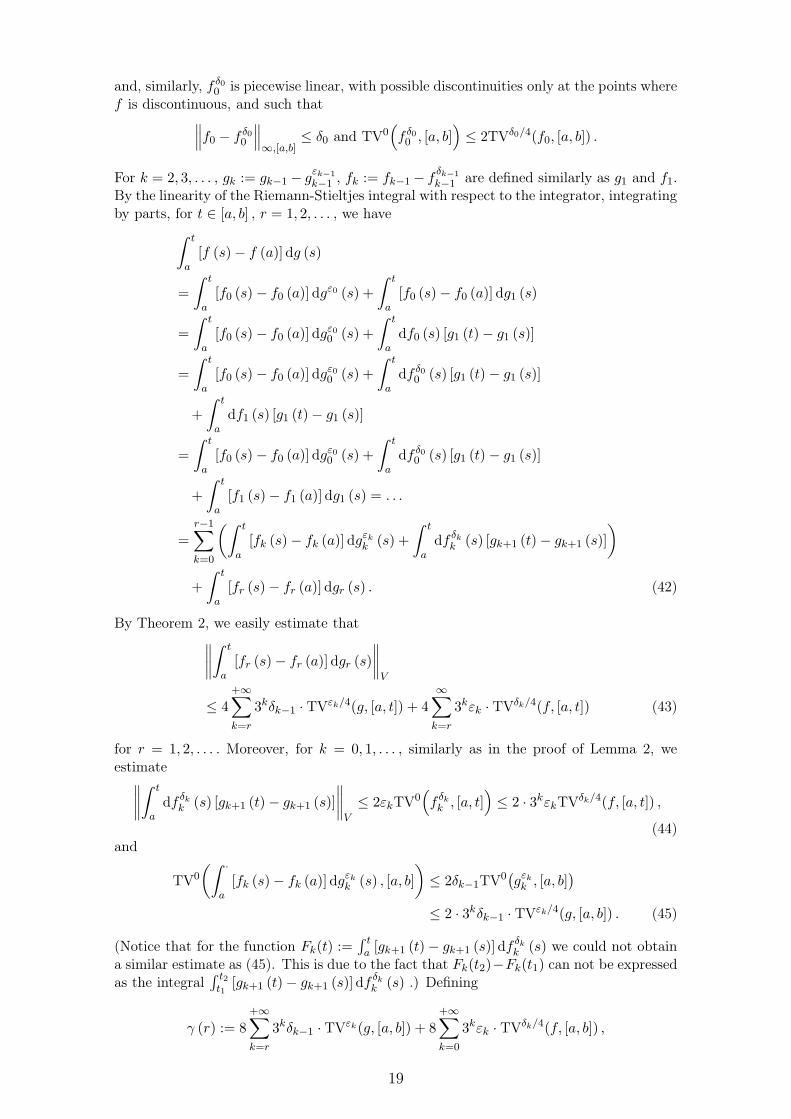
and, similarly, f δ00 is piecewise linear, with possible discontinuities only at the points where

f is discontinuous, and such that∥

∥

∥f0 − f δ0

0

∥

∥

∥

∞,[a,b]≤ δ0 and TV0

(

f δ00 , [a, b]

)

≤ 2TVδ0/4(f0, [a, b]) .

For k = 2, 3, . . . , gk := gk−1 − gεk−1

k−1 , fk := fk−1 − fδk−1

k−1 are defined similarly as g1 and f1.By the linearity of the Riemann-Stieltjes integral with respect to the integrator, integratingby parts, for t ∈ [a, b] , r = 1, 2, . . . , we have

ˆ t

a[f (s)− f (a)] dg (s)

=

ˆ t

a[f0 (s)− f0 (a)] dg

ε0 (s) +

ˆ t

a[f0 (s)− f0 (a)] dg1 (s)

=

ˆ t

a[f0 (s)− f0 (a)] dg

ε00 (s) +

ˆ t

adf0 (s) [g1 (t)− g1 (s)]

=

ˆ t

a[f0 (s)− f0 (a)] dg

ε00 (s) +

ˆ t

adf δ0

0 (s) [g1 (t)− g1 (s)]

+

ˆ t

adf1 (s) [g1 (t)− g1 (s)]

=

ˆ t

a[f0 (s)− f0 (a)] dg

ε00 (s) +

ˆ t

adf δ0

0 (s) [g1 (t)− g1 (s)]

+

ˆ t

a[f1 (s)− f1 (a)] dg1 (s) = . . .

=r−1∑

k=0

(ˆ t

a[fk (s)− fk (a)] dg

εkk (s) +

ˆ t

adf δk

k (s) [gk+1 (t)− gk+1 (s)]

)

+

ˆ t

a[fr (s)− fr (a)] dgr (s) . (42)

By Theorem 2, we easily estimate that∥

∥

∥

∥

ˆ t

a[fr (s)− fr (a)] dgr (s)

∥

∥

∥

∥

V

≤ 4+∞∑

k=r

3kδk−1 · TVεk/4(g, [a, t]) + 4∞∑

k=r

3kεk · TVδk/4(f, [a, t]) (43)

for r = 1, 2, . . . . Moreover, for k = 0, 1, . . . , similarly as in the proof of Lemma 2, weestimate∥

∥

∥

∥

ˆ t

adf δk

k (s) [gk+1 (t)− gk+1 (s)]

∥

∥

∥

∥

V

≤ 2εkTV0(

f δkk , [a, t]

)

≤ 2 · 3kεkTVδk/4(f, [a, t]) ,

(44)and

TV0

(ˆ ·

a[fk (s)− fk (a)] dg

εkk (s) , [a, b]

)

≤ 2δk−1TV0(

gεkk , [a, b])

≤ 2 · 3kδk−1 · TVεk/4(g, [a, b]) . (45)

(Notice that for the function Fk(t) :=´ ta [gk+1 (t)− gk+1 (s)] df

δkk (s) we could not obtain

a similar estimate as (45). This is due to the fact that Fk(t2)−Fk(t1) can not be expressedas the integral

´ t2t1

[gk+1 (t)− gk+1 (s)] dfδkk (s) .) Defining

γ (r) := 8

+∞∑

k=r

3kδk−1 · TVεk(g, [a, b]) + 8

+∞∑

k=0

3kεk · TVδk/4(f, [a, b]) ,

19

from (42), (44) and (43) we get

∥

∥

∥

∥

∥

ˆ t

a[f (s)− f (a)] dg (s)−

r−1∑

k=0

ˆ t

a[fk (s)− fk (a)] dg

εkk (s)

∥

∥

∥

∥

∥

V

≤r−1∑

k=0

∥

∥

∥

∥

ˆ t

adf δk

k (s) [gk+1 (t)− gk+1 (s)]

∥

∥

∥

∥

V

+

∥

∥

∥

∥

ˆ t

a[fr (s)− fr (a)] dgr (s)

∥

∥

∥

∥

V

≤ 1

2γ (r)

for any t ∈ [a, b] . Let us notice that by the very definition of the truncated variation,

TVγ

(ˆ ·

a[f (s)− f (a)] dg (s) , [a, t]

)

is bouned from above by the variation of any function approximating the indefinite integral´ ·a [f (s)− f (a)] dg (s) with accuracy γ/2. By this variational property of the truncated

variation and by (45) we get

TVγ(r)

(ˆ ·

a[f (s)− f (a)] dg (s) , [a, b]

)

≤ TV0

(

r−1∑

k=0

ˆ ·

a[fk (s)− fk (a)] dg

εkk (s) , [a, b]

)

≤ 2

r−1∑

k=0

3kδk−1 · TVεk/4(g, [a, b]) .

Proceeding with r to +∞ we get the assertion. �

Now we are ready to prove Theorem 3.Proof. Let γ > 0. We choose

α =

√

(q − 1)(p − 1) + 1

2, δ−1 =

1

2sup

a≤t≤b‖f (t)− f (a)‖L(E,V )

and define β by the equality

2 · 4p(

+∞∑

k=0

3k+1−p−α(1−α)(α2/[(q−1)(p−1)])k/(q−1)

)

‖f‖pp−TV,[a,b] δ1−p−1 β = γ.

Now, for k = 0, 1, . . . , we define

δk−1 = 3−(α2/[(q−1)(p−1)])

k+1δ−1,

εk = 3−(α2/[(q−1)(p−1)])

kα/(q−1)β.

Using (25), similarly as in the proof of Corollary 1 we estimate

+∞∑

k=0

3kδk−1 · TVεk/4(g, [a, b])

≤ 4q−1

(

+∞∑

k=0

3k+1−(1−α)(α2/[(q−1)(p−1)])k

)

‖g‖qq−TV,[a,b] δ−1β1−q

20

and

γ̃ : = 8

+∞∑

k=0

3kεk · TVδk/4(f, [a, b])

≤ 2 · 4p(

+∞∑

k=0

3k+1−p−α(1−α)(α2/[(q−1)(p−1)])k/(q−1)

)

‖f‖pp−TV,[a,b] δ1−p−1 β

= γ.

By the monotonicity of the truncated variation, Lemma 3 and the last two estimates weget

TVγ

(ˆ ·

a[f (s)− f (a)] dg (s) , [a, b]

)

≤ TVγ̃

(ˆ ·

a[f (s)− f (a)] dg (s) , [a, b]

)

≤ 4+∞∑

k=0

3kδk−1 · TVεk(g, [a, b])

≤ 4q

(

+∞∑

k=0

3k+1−(1−α)(α2/[(q−1)(p−1)])k

)

‖g‖qq−TV,[a,b] δ−1β1−q

= D̃p,q ‖f‖pq−pp−TV,[a,b] ‖f‖

p+q−pqosc,[a,b] ‖g‖

qq−TV,[a,b] γ

1−q,

where

D̃p,q =4q

(

+∞∑

k=0

3k+1−(1−α)(α2/[(q−1)(p−1)])k

)

×(

2 · 4p(

+∞∑

k=0

3k+1−p−α(1−α)(α2/[(q−1)(p−1)])k/(q−1)

))q−1

.

From this and the definition of ‖·‖q−TV,[a,b] we get

∥

∥

∥

∥

ˆ ·

a[f (s)− f (a)] dg (s)

∥

∥

∥

∥

q−TV,[a,b]

≤ Dp,q ‖f‖p−p/qp−TV,[a,b] ‖f‖

p/q+1−posc,[a,b] ‖g‖q−TV,[a,b] ,

where Dp,q = D̃1/qp,q . �

References

[1] M. Blumenthal, R. and R. K. Getoor. Some theorems on stable processes. Trans.Amer. Math. Soc., 95:263–273, 1960.

[2] Jean Dieudonné. Foundations of Modern Analysis, 3rd (enlarged and corrected) print-ing, volume 10 of Pure and Applied Mathematics. Academic Press, New York, 1969.

[3] Richard M. Dudley and Rimas Norvaiša. Concrete Functional Calculus. SpringerMonographs in Mathematics. Springer, New York, 2010.

[4] A. M. D’yačkov. Conditions for the existence of Stieltjes integral of functions ofbounded generalized variation. Anal. Math. (Budapest), 14:295–313, 1988.

[5] R. M. Łochowski. A new theorem on the existence of the Riemann-Stieltjes in-tegral and an improved version of the Loéve-Young inequality. J. Inequal. Appl.,2015(378):1–16, 2015.

[6] R. M. Łochowski and R. Ghomrasni. The play operator, the truncated variation andthe generalisation of the Jordan decomposition. Math. Methods Appl. Sci., 38(3):403–419, 2015.

21

[7] R. M. Łochowski and P. Miłoś. Limit theorems for the truncated variation andfor numbers of interval crossings of Lévy and self-similar processes. Preprint,http://akson.sgh.waw.pl/~rlocho/level_cross_Levy.pdf, 2014.

[8] T. Lyons. Differential equations driven by rough signals (I): an extension of an in-equality of L. C. Young. Math. Res. Lett., 1:451–464, 1994.

[9] Terry J. Lyons, Michael Caruana, and Thierry Lévy. Differential Equations DrivenBy Rough Paths, volume 1902 of Lecture Notes in Mathematics. Springer Verlag,Berlin, Heidelberg, 2007.

[10] G. Tronel and A. A. Vladimirov. On BV-type hysteresis operators. Nonlinear Anal.Ser. A: Theory Methods., 39(1):79–98, 2000.

[11] V. Vovk. Rough paths in idealized financial markets. Lith. Math. J., 51:274–285,2011.

[12] L. C. Young. An inequality of the Hölder type, connected with Stieltjes integration.Acta Math., 67(1):251–282, 1936.

[13] L. C. Young. General inequalities for Stieltjes integrals and the convergence of Fourierseries. Math. Ann., 115:581–612, 1938.

22