a new item response theory model for estimating person
TRANSCRIPT
University of South FloridaScholar Commons
Graduate Theses and Dissertations Graduate School
January 2013
A New Item Response Theory Model forEstimating Person Ability and Item Parameters forMultidimensional Rank Order ResponsesJacob SeybertUniversity of South Florida, [email protected]
Follow this and additional works at: http://scholarcommons.usf.edu/etd
Part of the Psychology Commons
This Dissertation is brought to you for free and open access by the Graduate School at Scholar Commons. It has been accepted for inclusion inGraduate Theses and Dissertations by an authorized administrator of Scholar Commons. For more information, please [email protected].
Scholar Commons CitationSeybert, Jacob, "A New Item Response Theory Model for Estimating Person Ability and Item Parameters for Multidimensional RankOrder Responses" (2013). Graduate Theses and Dissertations.http://scholarcommons.usf.edu/etd/4942
A New Item Response Theory Model for Estimating Person Ability and Item Parameters
for Multidimensional Rank Order Responses
by
Jacob Seybert
A dissertation submitted in partial fulfillment of the requirements for the degree of
Doctor of Philosophy Department of Psychology
College of Arts and Sciences University of South Florida
Major Professor: Stephen Stark, Ph.D. Oleksandr Chernyshenko, Ph.D.
Michael Coovert, Ph.D. John Ferron, Ph.D. Paul Spector, Ph.D.
Joseph A. Vandello, Ph.D.
Date of Approval: November 26, 2013
Keywords: Forced Choice, Response Bias, Multidimensional IRT, Noncognitive Assessment, Aberrance, Faking
Copyright © 2013, Jacob Seybert

ACKNOWLEDGMENTS
I would like to thank my dissertation committee members, Oleksander Chernyshenko,
Michael Coovert, John Ferron, Paul Spector, Joseph Vandello, and, my major professor, Stephen
Stark. I owe a great deal of thanks to Steve for all of his insightful and patient guidance over my
years at USF. I would also like to thank my father and mother, Jack and JoAlice Seybert, for
their unwavering support on the long road to obtaining my Ph.D. Finally, I would like to
especially thank Vanessa Hettinger, whose love and encouragement I could not have done
without.
i
TABLE OF CONTENTS
List of Tables ................................................................................................................................. iv List of Figures ................................................................................................................................ vi Abstract ......................................................................................................................................... vii Chapter 1 Introduction .....................................................................................................................1 The Present Investigation .....................................................................................................4 Chapter 2 Approaches to Scoring Forced Choice Measures ...........................................................6 Classical Test Theory Methods ............................................................................................6 The Multi-Unidimensional Pairwise Preference Model ......................................................9 A Thurstonian Model for MFC Data .................................................................................12 Summary ............................................................................................................................15 Preview of Upcoming Chapters .........................................................................................15 Chapter 3 Recent Advances in IRT Modeling of Forced Choice Responses ................................17 The PICK Model for Most Like Responses .......................................................................18 The RANK Model for Rank Responses.............................................................................19 Application of the RANK Model .......................................................................................20 The Generalized Graded Unfolding Model. ..........................................................20 RANK Model Parameter Estimation based on the GGUM. ..................................22 Chapter 4 The Hyperbolic Cosine Model as an Alternative to the GGUM for Unidimensional Single-Statement Responses.......................................................25 The Hyperbolic Cosine Model for Unidimensional Single- Stimulus Responses ..............................................................................................27 A Special Case: The Simple HCM (SHCM) .....................................................................30 Advantages of the HCM and SHCM as a Basis for MFC Test Construction ....................32 Summary ............................................................................................................................33 Chapter 5 Hyperbolic Cosine Models for Multidimensional Forced Choice Responses: Introducing the HCM-PICK and HCM-RANK Models ......................................34 The HCM-PICK: A Hyperbolic Cosine Model for Most Like Responses ........................35 A Formulation for Tetrads .....................................................................................35 A General Formulation ..........................................................................................37 A Special Case: The Simple HCM-PICK (SHCM-PICK) ....................................38 HCM-PICK Response Functions ...........................................................................38
ii
The HCM-RANK: A Hyperbolic Cosine Model for Rank Order Responses ....................41 Summary and Preview .......................................................................................................43 Chapter 6 HCM-RANK Model Item and Person Parameter Estimation .......................................45 MCMC Estimation for the HCM-RANK and SHCM-RANK Models ..............................47 The MH-within Gibbs Algorithm ..........................................................................47 Chapter 7 Study 1: A Monte Carlo Study to Assess the Efficacy of HCM-RANK Parameter Estimation Methods ...................................................51 Study Design ......................................................................................................................52 Constructing MFC Measures for the Simulation ...............................................................53 Statement Parameter Data ......................................................................................53 Test Design ............................................................................................................54 Test Assembly ........................................................................................................55 Simulation Details ..............................................................................................................60 Generating Rank Responses for MFC Tetrads ......................................................60 Generating Single-Statement Responses for Statement Precalibration in Two-Stage Conditions ...........................................................61 Simulation Process in Direct Conditions ...............................................................61 Simulation Process in Two-Stage Conditions........................................................62 Indices of Estimation Accuracy .........................................................................................62 MCMC Estimation Prior Distributions and Initial Parameter Values ...............................64 MCMC Estimation Burn-In and Chain Length .................................................................65 Hypotheses .........................................................................................................................66 Chapter 8 Study 1 Results ..............................................................................................................68 Simulation Results .............................................................................................................68 Testing Study Hypotheses..................................................................................................75 Study 1 Result Summary and Preview...............................................................................79 Chapter 9 Study 2: Examining SHCM-Rank Trait Score Recovery using SME Location Estimates .............................................................................................82 Simulation Study ................................................................................................................84 Study Design ..........................................................................................................84 Simulation Procedure .............................................................................................84 Indices of Estimation Accuracy .........................................................................................85 Hypotheses .........................................................................................................................85 Chapter 10 Study 2 Results ............................................................................................................87 Testing Study Hypotheses..................................................................................................87 Study 2 Result Summary and Preview...............................................................................89 Chapter 11 Study 3: A Construct Validity Investigation of SHCM-RANK Scores ......................91 Participants and Measures..................................................................................................92 Analyses .............................................................................................................................94 Hypotheses .........................................................................................................................95
iii
Chapter 12 Study 3 Results ............................................................................................................97 Study 3 Result Summary .................................................................................................102 Chapter 13 Discussion of Implications for Application and Research ........................................103 Future Research ...............................................................................................................104 References ....................................................................................................................................107 Appendix A: Derivation of the HCM-PICK ................................................................................123 Appendix B: Single-Statement Item Content for Study 1 ...........................................................129 Appendix C: Single-Statement IPIP Item Content for Study 3 ...................................................135 Appendix D: 4-D MFC Tetrad Measure for Study 3 ...................................................................137
iv
LIST OF TABLES
Table 7.1. Dimension Specifications for the 4-D MFC Test .....................................................55 Table 7.2. Dimension Specifications for the 8-D MFC Test .....................................................56 Table 7.3. Test Specifications for the 4-Dimension Test ...........................................................57 Table 7.4. Test Specifications for the 8-Dimension Test ...........................................................58 Table 8.1. Statement Parameter Recovery Statistics for Each of the Experimental Conditions .................................................................................................................69 Table 8.2. Person Parameter Recovery Statistics for Each of the Experimental Conditions via Rank Responses ................................................................................70 Table 8.3. Person Parameter Recovery Statistics for Each of the Experimental Conditions via Single-Statement Responses .............................................................71 Table 8.4. MANOVA Table for Multivariate Tests of Between Subjects Effects for Study 1 Hypotheses 1 and 2 ................................................................................75 Table 8.5. Results for Univariate Tests of Between Subjects Effects for Study 1 Hypotheses 1 and 2 ...................................................................................................76 Table 8.6. MANOVA Table for Multivariate Tests of Between Subjects Effects for Study 1 Hypotheses 3 and 4 ................................................................................77 Table 8.7. MANOVA Table for Multivariate Tests of Between Subjects Effects for Study 1 Hypothesis 5...........................................................................................78 Table 8.8. Results for Univariate Tests of Between Subjects Effects for Study 1 Hypothesis 5..............................................................................................................79 Table 10.1. Study 2 Trait Recovery Results using Simulated SME Locations ...........................88 Table 10.2. MANOVA Table for Multivariate Tests of Between Subjects Effects for Study 2 Hypothesis 1...........................................................................................88
v
Table 10.3. Results for Univariate Tests of Between Subjects Effects for Study 2 Hypothesis 1..............................................................................................................88 Table 12.1. Study 3 Correlations Between Personality Facet Scores Obtained using Single- Statement Responses and MFC Responses Scored Three Ways ..............................99 Table 12.2. Study 3 Criterion-Related Validities of Personality Facets Obtained using Single-Statement Responses and MFC Responses Scored Three Ways ................101
vi
LIST OF FIGURES
Figure 3.1. Item response function for a two-option GGUM item...........................................22 Figure 4.1. Subjective response probability plot ......................................................................29 Figure 4.2. HCM item response functions with different latitudes of acceptance ...................31 Figure 5.1. HCM-PICK option response functions for a block item involving four statements measuring the same dimension ............................................................39 Figure 5.2. HCM-PICK option response function selecting statement A (δ = -1.00, τ = 0.80) over statement B (δ = 0.50, τ = 1.50) in a 2-dimensional pair ...............41 Figure 7.1. Test information functions for each dimension in the 4-D test conditions ............59 Figure 7.2. Test information functions for each dimension in the 8-D test conditions ............59 Figure 8.1. Average estimates of statement location and latitude of acceptance parameters as a function of the corresponding generating parameter value for 4-D HCM-RANK conditions..................................................................72 Figure 8.2. Average estimates of statement location and latitude of acceptance parameters as a function of the corresponding generating parameter value for 8-D HCM-RANK conditions..................................................................73 Figure 8.3. Average estimates of statement location parameters as a function of the corresponding generating parameter value for 4-D and 8-D SHCM-RANK conditions ...............................................................................................................74 Figure 8.4. The interaction between statement parameters and estimation strategy for Study 1 conditions..................................................................................................79 Figure 10.1. Linear trend results for root mean square error (RMSE) and correlation statistics across Study 2 conditions ........................................................................89
vii
ABSTRACT
The assessment of noncognitive constructs poses a number of challenges that set it apart
from traditional cognitive ability measurement. Of particular concern is the influence of response
biases and response styles that can influence the accuracy of scale scores. One strategy to address
these concerns is to use alternative item presentation formats (such as multidimensional forced
choice (MFC) pairs, triads, and tetrads) that may provide resistance to such biases. A variety of
strategies for constructing and scoring these forced choice measured have been proposed, though
they often require large sample sizes, are limited in the way that statements can vary in location,
and (in some cases) require a separate precalibration phase prior to the scoring of forced-choice
responses. This dissertation introduces new item response theory models for estimating item and
person parameters from rank-order responses indicating preferences among two or more
alternatives representing, for example, different personality dimensions. Parameters for this new
model, called the Hyperbolic Cosine Model for Rank order responses (HCM-RANK), can be
estimated using Markov chain Monte Carlo (MCMC) methods that allow for the simultaneous
evaluation of item properties and person scores. The efficacy of the MCMC parameter estimation
procedures for these new models was examined via three studies. Study 1 was a Monte Carlo
simulation examining the efficacy of parameter recovery across levels of sample size,
dimensionality, and approaches to item calibration and scoring. It was found that estimation
accuracy improves with sample size, and trait scores and location parameters can be estimated
reasonably well in small samples. Study 2 was a simulation examining the robustness of trait
estimation to error introduced by substituting subject matter expert (SME) estimates of statement

viii
location for MCMC item parameter estimates and true item parameters. Only small decreases in
accuracy relative to the true parameters were observed, suggesting that using SME ratings of
statement location for scoring might be a viable short-term way of expediting MFC test
deployment in field settings. Study 3 was included primarily to illustrate the use of the newly
developed IRT models and estimation methods with real data. An empirical investigation
comparing validities of personality measures using different item formats yielded mixed results
and raised questions about multidimensional test construction practices that will be explored in
future research. The presentation concludes with a discussion of MFC methods and potential
applications in educational and workforce contexts.
1
CHAPTER 1:
INTRODUCTION
The past two decades have shown an increased interest in the assessment of noncognitive
constructs due to their ability to predict educational and organizational outcomes beyond
cognitive ability alone (Hough & Dilchert, 2010; Viswesvaran, Deller, & Ones, 2007).
Constructs such as conscientiousness have been shown to predict both task (Campbell, 1990) and
citizenship performance (Borman & Motowidlo, 1997) and may have the advantage of reducing
adverse impact that results from the use of measures of cognitive ability (Sackett, Schmitt,
Ellingson, & Kabin, 2001). Similarly, in education there is increased interest in examining
noncognitive factors, such as academic self-efficacy, need for cognition, and emotional
intelligence, and their relationships with educational and achievement outcomes (Richardson,
Abraham, & Bond, 2012). Yet another area of interest to researchers is the cross-cultural
comparison of relationships between noncognitive constructs and outcomes, such as job
performance, educational achievement, and life satisfaction (Diener & Diener, 2009; Frenzel,
Thrash, Pekrun, & Götz, 2007; Taras, Kirkman, & Steel, 2010). The inclusion of noncognitive
variables in education and organizational research may both increase the prediction efficacy of
success in these areas and facilitate understanding of these variables across situational and
cultural settings.
Despite these many potential benefits, noncognitive assessment involves a number of
challenges that set it apart from cognitive ability assessment. Of particular concern is the
influence of response biases and response styles on test scores (McGrath, Mitchell, Kim, &
2
Hough, 2010; Paulhus, 1991). The predominant approach to measuring noncognitive constructs
in organizational and research settings is to present a respondent with a series of descriptors or
statements, often transparent as to what is being measured, with instructions to indicate his or her
level of agreement (Likert, 1932). This approach has been shown to be susceptible to systematic
response biases, with central tendency, extreme response, halo, and socially desirable responding
influencing the accuracy of scale scores (Murphy, Jako, & Anhalt, 1993; Van Herk, Poortinga, &
Verhallen, 2004). Issues of central tendency and extreme response styles are common in cross
cultural research and reduce or distort the relationship between a construct and the outcome of
interest (Fischer, 2004). For example, recent research has suggested that cross-cultural
differences in response styles may explain the contradictory findings of a positive within-country
relationship between self-concept and academic achievement, but a negative relationship when
examined between countries (Cheung & Rensvold, 2000; Van da gaer, Grisay, Schulz, &
Gebhardt, 2012; Wilkins, 2004). In organizational contexts, socially desirable responding can
substantially elevate or depress noncognitive test scores, which particularly alters the rank order
of examinees at the extremes of the trait continua and reduces the utility of tests for decision
making (Christiansen, Goffin, Johnston, & Rothstein, 1994; Rosse, Stecher, Miller, & Levin,
1998; Stewart, Darnold, Zimmerman, Parks, & Dustin, 2010; Zickar, Rosse, Levin, & Hulin,
1996).
To address these concerns, researchers have examined alternative item presentation
formats that may provide resistance to such biases (Borman et al., 2001; Brown & Maydeu-
Olivares, 2012; Christiansen, Burns, Montgomery, 2005; Drasgow, Stark, & Chernyshenko,
2011; Heggestad, Morrison, Reeve, & McCloy., 2006; Jackson, 2001; Stark, 2002; Stark,
Chernyshenko, & Drasgow, 2005; Stark, Chernyshenko, Drasgow, & White, 2012; Stark,
3
Chernyshenko, Drasgow, White, Heffner, & Hunter, 2008). Multidimensional forced choice
pairs, triads, and tetrads are popular examples. Rather than asking respondents to indicate their
level of agreement with individual statements, statements representing different constructs are
presented in groups and respondents are instructed to pick or rank the statements in each group
from most to least like me (Stark, Chernyshenko, & Drasgow, 2011).
Multidimensional forced choice (MFC) measures have been used across a range of
research and applied settings for assessing personality (Stark, Chernyshenko, & Drasgow, 2008;
White & Young, 1998), vocational interest (SHL, 2006), and supervisor ratings of job
performance (Bartram, 2007; Borman et al., 2001). A number of strategies for constructing and
scoring MFC measures have been explored, ranging from summative scoring rules (Hicks, 1970;
Hirsh & Peterson, 2008; White & Young, 1998) to those based on factor analytic and item
response theory approaches (Maydeu-Olivares & Böckenholt, 2005; Maydeu-Olivares & Brown,
2010; Stark, 2002; Stark et al., 2005). These approaches, however, are not without limitations.
Scores obtained through summative strategies cannot be used to make inter-individual
comparisons due to the ipsativity resulting from the responses (Baron, 1996; Heggestad et al.,
2006; Hicks, 1970; Meade, 2004; Stark, 2002; Stark et al., 2005), and factor analytic and item
response theory strategies require large sample sizes and (in some cases) a two-stage approach
requiring a separate precalibration of single-statement parameters prior to the scoring of forced-
choice responses. Consequently, the application of MFC items in practice and research would
benefit from a construction and scoring strategy for which scores can be obtained under
conditions of small sample size and potentially streamlined through the incorporation of subject
matter expert (SME) ratings into the scale development and scoring process.
4
The Present Investigation
Forced choice items can vary in their composition and response instructions, resulting in
the development of different models to account for the variety of types. Pairwise preference
models have been developed for unidimensional item responses (e.g., Andrich, 1995; Stark &
Drasgow, 2002; Zinnes & Griggs, 1974) and multidimensional pairs (e.g., Stark et al., 2005;
Zinnes & Griggs, 1974), in addition to models for item tetrads (e.g., Brown & Maydeu-Olivares,
2011; Brown & Maydeu-Olivares, 2013; de la Torre, Ponsoda, Leenen, & Hontangas, 2012).
Although recent research has made significant advances in the scoring of these items, there is
still a need for a model which can address a range of MFC formats, has item and person
parameters which can be efficiently estimated, and that can be easily implemented in applied
settings.
This paper will introduce a model for estimating item and person parameters from data
collected via the rank-ordering of statements presented in a MFC format. Working from Luce’s
(1959) theory of choice behavior, the Hyperbolic Cosine Model (HCM; Andrich & Luo, 1993)
for single-stimulus data will be extended to the multidimensional forced choice case. This new
model, called the Hyperbolic Cosine Model for Rank order responses (HCM-RANK), provides
the basis for the recovery of both person trait estimates and item parameter estimates directly
from rank-order responses. A special case of this model, the Simple HCM-RANK (SHCM-
RANK), is particularly attractive because each statement in a forced choice item is represented
by just one location or extremity parameter, which might be estimated using subject matter
experts (SMEs) judgments in the early stages of testing.
The following chapters will provide an overview of the use of forced choice measures in
noncognitive assessment and the methods that have been developed for scoring and item

5
analysis. Next, recent advances in the scoring of MFC items and assumptions about the
underlying response process will be reviewed. The HCM as a model for single-stimulus (i.e.,
single statement) responses will be described, and the HCM-RANK model for MFC rank
responses will be derived. Following a detailed description of the HCM-RANK parameter
estimation procedures, Study 1 will explore parameter recovery using a Monte Carlo simulation
that varies sample size, dimensionality, and approaches to item calibration and scoring. A second
simulation, Study 2, will examine the robustness of trait score estimation to error introduced by
substituting subject matter expert (SME) estimates of statement location for true parameters.
Study 3 will illustrate the use of the newly developed IRT models and MCMC estimation
methods with real data, and the presentation will conclude with a discussion of potential MFC
applications in educational and workforce contexts.
6
CHAPTER 2:
APPROACHES TO SCORING FORCED CHOICE MEASURES
Forced choice measures have been explored by applied psychologists for noncognitive
testing since the late 1930s (e.g., Strong Vocational Interest Blank, Strong, 1938; Gordon
Personal Profile, Gordon, 1953). However, concerns about ipsativity have, until recently,
impeded widespread use in organizations. Classical test theory methods of scoring, in which a
point is awarded for endorsing an option in a forced choice item, generally lead to ipsative data
characterized by total scores that sum to a constant across dimensions and negative scale
correlations (Hicks, 1970; Meade, 2004; Stark, 2002; Stark, Chernyshenko, & Drasgow, 2005).
However, research over the last two decades has produced several efficacious ways of deriving
normative information from multidimensional forced choice (MFC) measures (Brown &
Maydeu-Olivares, 2011; de la Torre et al., 2012; Stark, Chernyshenko, & Drasgow, 2005), and
research showing that MFC measures are more resistant than single statement measures to
response biases, such as rating scale errors (Borman et al., 2001) and socially desirable
responding (Jackson, Wroblewski, & Ashton, 2000; Stark, Chernyshenko, Drasgow, White,
Heffner, & Hunter, 2008; Stark, Chernyshenko, & Drasgow, 2010; Stark, Chernyshenko, &
Drasgow, 2011), has reinvigorated interest for personnel screening applications.
Classical Test Theory Methods
Beginning in the mid-1990s, there were several key research developments that laid the
foundation for modern MFC testing and the research conducted for this dissertation. The first
breakthrough came from the U.S. Army Research Institute’s Assessment of Individual
7
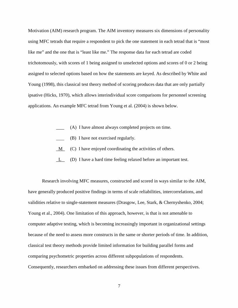
Motivation (AIM) research program. The AIM inventory measures six dimensions of personality
using MFC tetrads that require a respondent to pick the one statement in each tetrad that is “most
like me” and the one that is “least like me.” The response data for each tetrad are coded
trichotomously, with scores of 1 being assigned to unselected options and scores of 0 or 2 being
assigned to selected options based on how the statements are keyed. As described by White and
Young (1998), this classical test theory method of scoring produces data that are only partially
ipsative (Hicks, 1970), which allows interindividual score comparisons for personnel screening
applications. An example MFC tetrad from Young et al. (2004) is shown below.
(A) I have almost always completed projects on time.
(B) I have not exercised regularly.
M (C) I have enjoyed coordinating the activities of others.
L
(D) I have a hard time feeling relaxed before an important test.
Research involving MFC measures, constructed and scored in ways similar to the AIM,
have generally produced positive findings in terms of scale reliabilities, intercorrelations, and
validities relative to single-statement measures (Drasgow, Lee, Stark, & Chernyshenko, 2004;
Young et al., 2004). One limitation of this approach, however, is that is not amenable to
computer adaptive testing, which is becoming increasingly important in organizational settings
because of the need to assess more constructs in the same or shorter periods of time. In addition,
classical test theory methods provide limited information for building parallel forms and
comparing psychometric properties across different subpopulations of respondents.
Consequently, researchers embarked on addressing these issues from different perspectives.
8
Stark, Chernyshenko, and Drasgow developed an item response theory (IRT) approach to MFC
test construction and scoring using a multidimensional pairwise preference format, which
requires respondents to choose the one statement in each pair that is more like me (Stark, 2002;
Stark, Chernyshenko, & Drasgow, 2005; Stark, Chernyshenko, Drasgow, & White, 2012).
Böckenholt (2001, 2004) developed confirmatory factor analytic (CFA) methods for scoring
unidimensional pairwise preference items, and Maydeu-Olivares and Brown (2010) began
developing CFA methods for constructing and scoring MFC tests involving more complex item
formats, such as triads or tetrads (e.g., OPQ32i; SHL, 2006), which require respondents to rank
response alternatives from most to least like me. Later, de la Torre, Ponsada, and colleagues
(2012) generalized Stark’s (2002) approach for use with more complex formats and developed
Markov chain Monte Carlo (MCMC) estimation methods for simultaneously calibrating and
scoring MFC items, which facilitates traditional IRT methods of item analysis, equating, and
differential item functioning detection.
The remainder of this chapter describes the Stark et al. and Maydeu-Olivares and Brown
approaches to MFC test construction and scoring. The next chapter describes de la Torre et al.’s
models for MFC responses, which subsume Stark’s (2002) model as a special case. Following
are several chapters devoted to the topic of this dissertation. In short, I describe the development
and evaluation of a new model for MFC testing applications, which capitalizes on the
technological advances attributable to de la Torre et al., while incorporating features that may
ultimately improve and accelerate the process of MFC test development and launch for
organizational applications.
9
The Multi-Unidimensional Pairwise Preference Model
Stark (2002) proposed an IRT method for MFC test construction and scoring that was
designed to overcome ipsativity and provide a foundation for computerized adaptive testing
applications. Rather than using item tetrads, he adopted a pairwise preference format because it
was a logical extension of the unidimensional pairwise preference research conducted previously
in the context of performance appraisal (Borman et al., 2001; Stark & Drasgow, 2002) and it was
more mathematically tractable for this initial foray into IRT MFC test construction and scoring.
Pairwise preference items were also selected to simplify the response process for participants,
because research underway at the time suggested that tetrads have a higher “cognitive load,”
which may cause examinee fatigue and potentially reduce the incremental validities over
cognitive ability measures (Böckenholt, 2004; Christiansen, Burns, Montgomery, 2005;
Converse, Oswald, Imus, Hedricks, Roy, & Butera, 2008; Vasilopoulos, Cucina, Dyomina,
Morewitz, & Reilly, 2006).
Stark’s model, now referred to as the multi-unidimensional pairwise preference model
(MUPP; Stark, Chernyshenko, & Drasgow, 2005), assumes that when presented with a pair of
statements, representing the same or different constructs, a respondent evaluates each statement
and makes independent decisions about agreement. Formally, the probability of preferring
statement s to statement t in a pairwise preference item is given by:
𝑃(𝑠 > 𝑡)𝑖�θ𝑑𝑠 , θ𝑑𝑡� = 𝑃𝑠𝑡{1,0}
𝑃𝑠𝑡{1,0}+𝑃𝑠𝑡{0,1} = 𝑃𝑠(1)𝑃𝑡(0)𝑃𝑠(1)𝑃𝑡(0)+𝑃𝑠(0)𝑃𝑡(1), (2.1)
where:
i = the index for each pairwise preference item, where i = 1 to I;
s, t = the indices for the first and second statements, respectively, in an item;
10
d = the dimension associated with a given statement, where d = 1, … , D;
θ𝑑𝑠 , θ𝑑𝑡 = the latent trait values for a respondent on dimensions ds and dt, respectively;
𝑃𝑠𝑡{1,0} = the joint probability of selecting statement s, and not selecting statement t;
𝑃𝑠𝑡{0,1} = the joint probability of selecting statement t, and not selecting statement s;
𝑃𝑠(1), 𝑃𝑡(1) = the probabilities of endorsing statements s and t, respectively;
𝑃𝑠(0), 𝑃𝑡(0) = the probabilities of not endorsing statements s and t, respectively; and
𝑃(𝑠 > 𝑡)𝑖�θ𝑑𝑠 , θ𝑑𝑡� = the probability of a respondent preferring statement s to statement t
in pairwise preference item i.
This formulation of pairwise preference probability is notably similar to Andrich’s (1995)
definition for unidimensional pairwise preferences.
Stark (2002) described and evaluated a two-stage approach to MFC test construction and
scoring. First, write noncognitive statements ranging in extremity from low to medium to high on
the constructs to be assessed. Administer the statements to large samples of respondents with
instructions to indicate their levels of agreement using an ordered polytomous response format.
Dichotomize the polytomous data and estimate statement parameters using an IRT model for
single-statement responses that provides adequate model-data fit. Based on research at the time,
Stark chose the Generalized Graded Unfolding model (Roberts, Donoghue, & Laughlin, 2000) as
the basis for test construction and scoring, although many other ideal point and dominance
models could have been selected. After estimating statement parameters using the GGUM,
obtain social desirability ratings for MFC item creation by re-administering the statements in the
context of a “fake good” study (White & Young, 1998) or by collecting subject matter expert
ratings. Next, form multidimensional pairwise preference items by pairing statements similar in
11
social desirability from different dimensions, and assemble MFC test forms by combining
multidimensional pairs with a small percentage of similarly matched unidimensional pairs to
identify the metric of trait scores. Scoring multidimensional pairwise preference tests is then
accomplished by multidimensional Bayes modal estimation, via the substitution of observed
responses and GGUM statement parameters into Equation 2.1 for pairwise preference response
probabilities. For future adaptive testing applications, Stark (2002) provided item and test
information equations that could be used to create and select items that are optimal for individual
examinees, subject to content constraints, at any point during an exam.
Stark (2002) and Stark, Chernyshenko, and Drasgow (2005) conducted Monte Carlo
simulations to examine trait score recovery with MFC tests of different lengths, dimensionality,
and percentages of unidimensional pairings. Overall, they found good to excellent recovery of
trait scores with 20% or fewer unidimensional pairings, but the standard errors produced by the
multidimensional minimization procedure were too conservative. Stark, Chernyshenko,
Drasgow, and White (2012) reported follow-up simulations comparing nonadaptive and adaptive
MFC testing with as many as 25 dimensions and, consistent with expectations, they found that
adaptive testing yielded trait score recovery statistics comparable to nonadaptive tests that were
nearly twice as long, scoring was robust to moderate violations of the assumptions of
independent normal prior distributions, and a replication-based method of estimating standard
errors for trait scores provided more accurate and stable results than those originally obtained
using the approximated inverse Hessian.
Since the advent of this methodology, organizational research has focused on validating
multidimensional pairwise preference assessments in various laboratory and field settings (e.g.,
Chernyshenko, Stark, Prewett, Gray, Stilson, & Tuttle, 2009; Knapp, & Heffner, 2009; Drasgow,
12
Stark, Chernyshenko, Nye, Hulin, & White, 2012; Knapp, Heffner, & White, 2011; Stark,
Chernyshenko, & Drasgow, 2011), generalizing the psychometric model to more complex item
formats and improving methods for estimating MFC item parameters and trait scores (de la
Torre, Ponsoda, Leenen, & Hontangas, 2012). Research involving simpler unidimensional
models has also sparked speculation that the successful use of subject matter expert ratings of
statement extremity for unidimensional pairwise preference test construction and scoring (Stark,
Chernyshenko, & Guenole, 2011) can provide a reasonable initial alternative to MFC item
parameter estimation, which would dramatically reduce the costs of item pretesting with large
samples. Research by Seybert and colleagues has also explored methods for calibrating and
scoring unidimensional ideal point single-statement responses using an alternative model to the
GGUM – namely Andrich’s Hyperbolic Cosine Model (HCM; Andrich & Luo, 1993) and its
variations – with the intent of providing an alternative, more tractable basis for MFC test
construction and scoring.
A Thurstonian Model for MFC Data
Maydeu-Olivares and Brown developed a confirmatory factor analytic (CFA) method for
collecting and scoring MFC responses in accordance with Thurstone’s (1927) law of
comparative judgment (Brown, 2010; Brown & Maydeu-Olivares, 2011, 2013; Maydeu-
Olivares, 2001; Maydeu-Olivares & Brown, 2010). For example, when presented with a MFC
item tetrad, rather than asking respondents to indicate the statements in each group that are most
and least like me, respondents are instructed to rank the statements based on their level of
agreement or preference, with 1 being the most preferred and 4 being the least preferred, as
shown:
13
2 A. I have almost always completed projects on time.
3 B. I have not exercised regularly.
1 C. I have enjoyed coordinating the activities of others.
4
D. I have a hard time feeling relaxed before an important test.
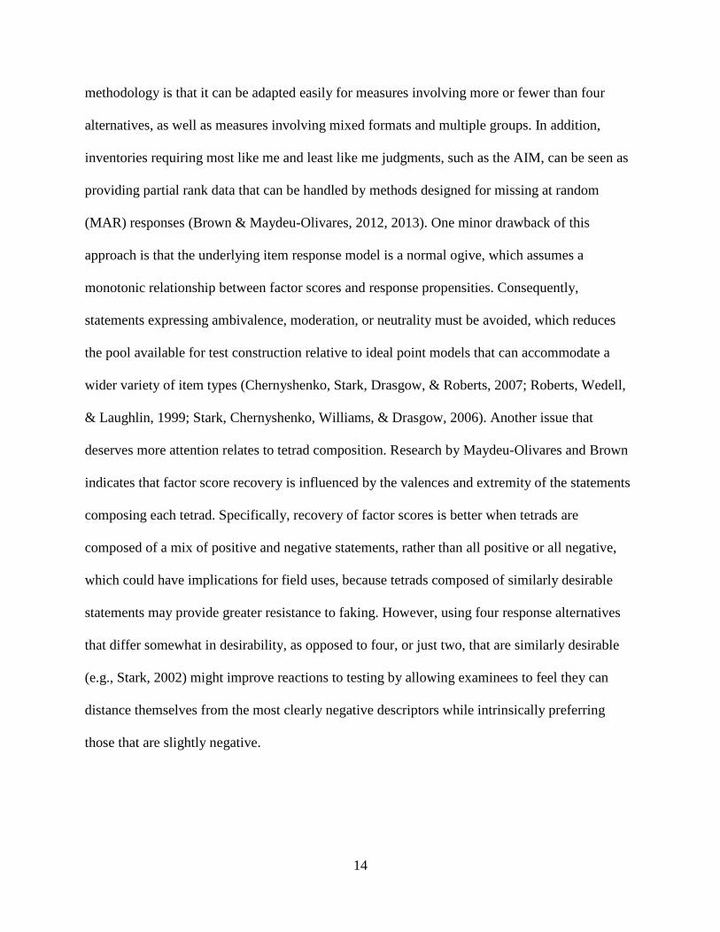
Assuming transitivity, the ranks are decomposed into a series of dichotomously (0, 1) scored
pairwise preference judgments, where the symbol > means “preferred to,” coded 1. In general,
for any set of M statements, there are M(M-1)/2 unique pairs. For tetrads, there are 6. For the
ranks indicated above, the six pairwise preference judgments would be scored dichotomously as
shown:
(𝐴 > 𝐵)
1
(𝐴 > 𝐶)
0
(𝐴 > 𝐷)
1
(𝐵 > 𝐶)
0
(𝐵 > 𝐷)
1
(𝐶 > 𝐷)
1
Brown and Maydeu-Olivares (2011) proposed scoring binary responses derived from
MFC rank data using a multidimensional normal ogive model, with local dependencies due to
statements appearing in the multiple pairs associated with each tetrad having constrained (equal)
factor loadings. Brown and Maydeu-Olivares (2013) provided Mplus syntax (Muthén & Muthén,
2010) to compute item loadings, item thresholds and factor scores, which are akin, respectively,
to item discrimination, item extremity, and person parameters (trait scores) in traditional IRT
terminology. For details on this CFA procedure, readers are encouraged to consult Brown et al.
(2011, 2013).
The Thurstonian approach to analyzing MFC rank data has proven effective in a wide
range of simulation conditions (Brown & Maydeu-Olivares, 2011). A strong point of this
14
methodology is that it can be adapted easily for measures involving more or fewer than four
alternatives, as well as measures involving mixed formats and multiple groups. In addition,
inventories requiring most like me and least like me judgments, such as the AIM, can be seen as
providing partial rank data that can be handled by methods designed for missing at random
(MAR) responses (Brown & Maydeu-Olivares, 2012, 2013). One minor drawback of this
approach is that the underlying item response model is a normal ogive, which assumes a
monotonic relationship between factor scores and response propensities. Consequently,
statements expressing ambivalence, moderation, or neutrality must be avoided, which reduces
the pool available for test construction relative to ideal point models that can accommodate a
wider variety of item types (Chernyshenko, Stark, Drasgow, & Roberts, 2007; Roberts, Wedell,
& Laughlin, 1999; Stark, Chernyshenko, Williams, & Drasgow, 2006). Another issue that
deserves more attention relates to tetrad composition. Research by Maydeu-Olivares and Brown
indicates that factor score recovery is influenced by the valences and extremity of the statements
composing each tetrad. Specifically, recovery of factor scores is better when tetrads are
composed of a mix of positive and negative statements, rather than all positive or all negative,
which could have implications for field uses, because tetrads composed of similarly desirable
statements may provide greater resistance to faking. However, using four response alternatives
that differ somewhat in desirability, as opposed to four, or just two, that are similarly desirable
(e.g., Stark, 2002) might improve reactions to testing by allowing examinees to feel they can
distance themselves from the most clearly negative descriptors while intrinsically preferring
those that are slightly negative.
15
Summary
The methods described in this chapter represent significant advances in the recent history
of MFC testing. The U.S. Army AIM research program (White & Young, 1998) produced a
classical test theory method of creating MFC tests that provides scores which can be used for
organizational decision making. This work was a springboard for many important research
studies (Heggestad, Morrison, Reeve, & McCloy, 2006; McCloy, Heggestad, & Reeve, 2005;
Stark, 2002; Stark, Chernyshenko, & Drasgow, 2005) and applications in organizations. The
MUPP approach to test construction and scoring (Stark, 2002) described how ipsativity and
faking in personality assessment could be addressed with modern psychometric theory. The
general model for pairwise preference judgments and the two-stage approach to test construction
and scoring laid a foundation for computer adaptive testing (CAT), which significantly reduces
testing time while maintaining scoring precision (Stark, Chernyshenko, & Drasgow, 2011; Stark
et al., 2012). The Thurstonian model (Brown, 2010; Brown & Maydeu-Olivares, 2011, 2013)
provides yet another rigorous and flexible framework for constructing and scoring MFC
measures. Although not ideal for CAT, it allows quicker deployment of MFC test forms by
eliminating the preliminary statement calibration phase proposed by Stark (2002). It is also
readily adapted to different item formats, and it can be implemented easily with widely available
statistical software.
Preview of Upcoming Chapters
Chapter 3 discusses more recent advances in modeling MFC tetrad responses from a
traditional IRT perspective. It provides a detailed review of de la Torre et al.’s PICK and RANK
models, which subsume Stark’s (2002) model for pairwise preferences, based on the GGUM.
Chapter 4 presents David Andrich’s Hyperbolic Cosine Model (HCM; Andrich & Luo, 1993) as

16
an alternative to the GGUM, which Seybert and colleagues have been exploring as an alternative
to the GGUM for noncognitive single-statement responses.
In Chapter 5, a new IRT model for MFC rank order responses that is the focus of this
dissertation is introduced. This new model, which is a generalization of the HCM and is
henceforth referred to as the Hyperbolic Cosine Model for Multidimensional Rank order
responses (HCM-RANK), has several interesting properties that make it an attractive alternative
to the GGUM-based PICK and RANK models, which are currently at the forefront of MFC
psychometric innovation. Chapter 6 then describes an estimation strategy to obtain parameter
estimates using the HCM-RANK.
Chapters 7 through 12 describe simulation studies and results that evaluate the efficacy of
MCMC parameter estimation methods developed for scoring HCM-RANK responses. In
addition, a study that explores using SME judgments of statement location in place of IRT
parameter estimates to expedite test development is described.
17
CHAPTER 3:
RECENT ADVANCES IN IRT MODELING OF FORCED CHOICE RESPONSES
The previous chapter presented two alternatives to classical test theory methods for
analyzing MFC responses. Although the methods differ in several ways, the data used for
parameter estimation in both cases stem from explicit or inferred pairwise preference judgments.
More specifically, whereas Stark (2002) presented a model designed for explicit pairwise
preferences and chose an ideal point model as the basis for parameter estimation, Maydeu-
Olivares and Brown proposed a general approach involving ranks. Assuming transitivity, they
recode ranks into a set of inferred pairwise preference judgments and estimate parameters via a
dominance (normal ogive) model.
An alternative conceptualization of ranks was provided by Luce (1959). Luce viewed
ranks as a series of independent preferential choice judgments among sets of successively fewer
alternatives. Assigning ranks involves a process, often referred to as decomposition (Yellott,
1980, 1997), which holds that when an individual ranks a set of alternatives, he or she makes the
first independent preferential choice from the full set, the second independent choice from the
remaining set, and so on, until the last rank is determined. This decomposition assumption
provides a straightforward alternative way of modeling MFC rank responses, as well as “most
like me” and/or “least like me” responses. The probability of a particular set of ranks is just the
product of the preferential choice probabilities at each stage of the decomposition. This logic is
central to de la Torre et al.’s (2012) PICK and RANK models for MFC item parameter
estimation and scoring, which are described below.
18
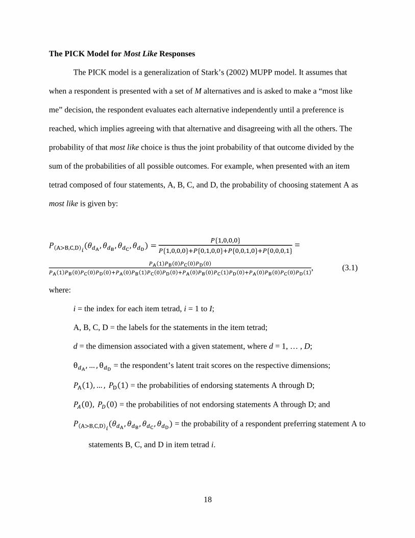
The PICK Model for Most Like Responses
The PICK model is a generalization of Stark’s (2002) MUPP model. It assumes that
when a respondent is presented with a set of M alternatives and is asked to make a “most like
me” decision, the respondent evaluates each alternative independently until a preference is
reached, which implies agreeing with that alternative and disagreeing with all the others. The
probability of that most like choice is thus the joint probability of that outcome divided by the
sum of the probabilities of all possible outcomes. For example, when presented with an item
tetrad composed of four statements, A, B, C, and D, the probability of choosing statement A as
most like is given by:
𝑃(A>B,C,D)𝑖(𝜃𝑑A ,𝜃𝑑B ,𝜃𝑑C ,𝜃𝑑D) =
𝑃{1,0,0,0}𝑃{1,0,0,0}+𝑃{0,1,0,0}+𝑃{0,0,1,0}+𝑃{0,0,0,1}
=
𝑃A(1)𝑃B(0)𝑃C(0)𝑃D(0)𝑃A(1)𝑃B(0)𝑃C(0)𝑃D(0)+𝑃A(0)𝑃B(1)𝑃C(0)𝑃D(0)+𝑃A(0)𝑃B(0)𝑃C(1)𝑃D(0)+𝑃A(0)𝑃B(0)𝑃C(0)𝑃D(1), (3.1)
where:
i = the index for each item tetrad, i = 1 to I;
A, B, C, D = the labels for the statements in the item tetrad;
d = the dimension associated with a given statement, where d = 1, … , D;
θ𝑑A , … , θ𝑑D = the respondent’s latent trait scores on the respective dimensions;
𝑃A(1), … , 𝑃D(1) = the probabilities of endorsing statements A through D;
𝑃𝐴(0), 𝑃𝐷(0) = the probabilities of not endorsing statements A through D; and
𝑃(A>B,C,D)𝑖(𝜃𝑑A ,𝜃𝑑B ,𝜃𝑑C ,𝜃𝑑D) = the probability of a respondent preferring statement A to
statements B, C, and D in item tetrad i.
19
Similarly, letting TOTAL represent the denominator of Equation 3.1 for convenience, the
probability of choosing statement B in the tetrad as most like is P{0,1,0,0}/TOTAL. The
probability of choosing statement C as most like is P{0,0,1,0}/TOTAL, and the probability of
choosing statement D as most like is P{0,0,0,1}/TOTAL.
Importantly, because choosing most like is synonymous with expressing a preference, and
the logic is the same regardless of the number of alternatives in a set, the PICK model can be
used to explain observed ranks for MFC item parameter estimation and scoring and to assign or
generate ranks for MFC data simulations. The sections immediately below introduce de la Torre
et al.’s RANK model, illustrate how assignment of ranks can be viewed as a sequence of PICK
applications, and provide details on how this model can be used to estimate the probabilities of
observed ranks, which are needed for MFC tetrad parameter estimation.
The RANK Model for Rank Responses
Following Luce (1959), de la Torre et al. (2012) assume that ranks can be decomposed
into a sequence of independent preference, or most like, judgments among sets of successively
fewer alternatives (M, M-1, …, 2). At each step in the decomposition process (Critchlow,
Flinger, & Verducci, 1991; Yellott, 1997), the PICK model can be used to compute most like
probabilities, and by the independence assumption, the probability of a set of ranks is therefore
just the product of the PICK probabilities.
Continuing with the item tetrad example from above, suppose the four statements
composing the tetrad are ranked A>D>B>C, where > means preferred. From this set of four,
three PICK probabilities are calculated:
1. 𝑃(A>B,C,D) = probability of selecting A as most like from the set of four;
2. 𝑃(D>B,C)) = probability of selecting D as most like from the remaining three; and
20
3. 𝑃(B>C) = probability of selecting B as most like from the remaining two.
The probability of the ranking A>D>B>C is equal to the product of the three PICK probabilities.
Formally, given a respondent’s trait scores for the dimensions represented by the statements,
𝑃(A>D>B>C)𝑖�𝜃𝑑A ,𝜃𝑑B ,𝜃𝑑C ,𝜃𝑑D� = 𝑃(A>B,C,D)𝑃(D>B,C)𝑃(B>C) (3.2)
The model presented in Equation 3.2 was labeled the RANK model by de la Torre et al.
(2012). Although this example illustrates most-to-least ranking, it has been noted that least-to-
most preferred ranks could also be assigned, and that might result in different probabilities and
selections at each stage (Luce, 1959).
Application of the RANK Model
The RANK model involves a series of PICK applications. Therefore, like the MUPP
model (Stark, 2002), a lower-level model is required for computing the underlying statement
agreement probabilities. In accordance with Stark (2002) and many recent studies showing good
fit of the Generalized Graded Unfolding Model (GGUM; Roberts, Donoghue, & Laughlin, 2000)
to single-statement noncognitive responses (Carter & Dalal, 2010; Chernyshenko et al., 2007;
Heggestad et al., 2006; Stark et al., 2006; Tay, Drasgow, Rounds, & Williams, 2009), de la Torre
et al. (2012) also selected the GGUM as the basis for developing and evaluating item parameter
estimation and scoring methods for MFC tetrad responses.
The Generalized Graded Unfolding Model. The GGUM is an ideal point model that
can be used for dichotomous and ordered polytomous responses. For PICK applications, the
dichotomous version is needed. Specifically, the GGUM is used to compute statement agreement
probabilities that underlie most like selections. Letting 𝑃(0) and 𝑃(1) represent the respective
21
probabilities of disagreeing (Z=0) and agreeing (Z=1) with a particular statement, given a
respondent’s latent trait score (𝜃) on the dimension that statement represents, and three
statement parameters (𝛼, 𝛿, 𝜏) reflecting discrimination, location (extremity), and threshold,
respectively, we have:
𝑃(0) = 𝑃(𝑍 = 0|𝜃) = 1+exp(𝛼[3(𝜃−𝛿)])γ
, and (3.3)
𝑃(1) = (𝑍 = 1|𝜃) = exp(𝛼[(𝜃−𝛿)−𝜏])+exp(𝛼[2(𝜃−𝛿)−𝜏])𝛾
, (3.4)
where :
γ = 1 + exp(𝛼[3(𝜃 − 𝛿)]) + exp(𝛼[(𝜃 − 𝛿) − 𝜏]) + exp(𝛼[2(𝜃 − 𝛿) − 𝜏]), is a
normalizing factor equal to the sum of the numerators of equations 3.3 and 3.4.
Ideal point models, such as the GGUM, assume that a comparison process governs the
decision to agree or disagree with a statement. Specifically, they assume a respondent estimates
the distance between his or her location and the location of the statement on the underlying trait
continuum. If the distance is small the respondent agrees with the statement. If the distance is
large the respondent disagrees. Thus, as the perceived distance between the person and the
statement increases, the probability of agreeing with the statement decreases. Ideal point models
can therefore have item response functions (IRFs), which portray the relationship between trait
scores and agreement probabilities, that are nonmonotonic and possibly bell-shaped.
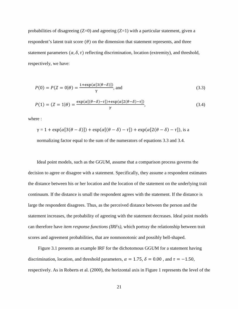
Figure 3.1 presents an example IRF for the dichotomous GGUM for a statement having
discrimination, location, and threshold parameters, 𝛼 = 1.75, 𝛿 = 0.00 , and 𝜏 = −1.50,
respectively. As in Roberts et al. (2000), the horizontal axis in Figure 1 represents the level of the
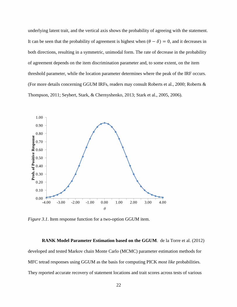
22
underlying latent trait, and the vertical axis shows the probability of agreeing with the statement.
It can be seen that the probability of agreement is highest when (𝜃 − 𝛿) = 0, and it decreases in
both directions, resulting in a symmetric, unimodal form. The rate of decrease in the probability
of agreement depends on the item discrimination parameter and, to some extent, on the item
threshold parameter, while the location parameter determines where the peak of the IRF occurs.
(For more details concerning GGUM IRFs, readers may consult Roberts et al., 2000; Roberts &
Thompson, 2011; Seybert, Stark, & Chernyshenko, 2013; Stark et al., 2005, 2006).
Figure 3.1. Item response function for a two-option GGUM item.
RANK Model Parameter Estimation based on the GGUM. de la Torre et al. (2012)
developed and tested Markov chain Monte Carlo (MCMC) parameter estimation methods for
MFC tetrad responses using GGUM as the basis for computing PICK most like probabilities.
They reported accurate recovery of statement locations and trait scores across tests of various
0.00
0.10
0.20
0.30
0.40
0.50
0.60
0.70
0.80
0.90
1.00
-4.00 -3.00 -2.00 -1.00 0.00 1.00 2.00 3.00 4.00
Prob
. of P
ositi
ve R
espo
nse
θ
23
lengths and numbers of dimensions. However, they used extremely tight priors on discrimination
and threshold parameters when estimating statement locations; essentially the discrimination and
threshold parameters were fixed at 1.00 and -1.00, respectively. Research is needed to determine
whether item parameter estimation accuracy can be maintained when these constraints are
relaxed and how different test design specifications affect estimation outcomes. It would also be
interesting to explore whether relaxing these constraints affects parameter estimation in the
absence of any unidimensional items, with and without repeating statements across tetrads. In
addition, it remains to be seen whether using an alternative ideal point model as the basis for
computing PICK probabilities can improve RANK estimation or streamline MFC test
deployment by reducing the sample sizes needed for item calibration.
The next chapter expands on this latter issue by introducing an alternative model as the
basis for computing PICK probabilities, namely Andrich’s Hyperbolic Cosine Model (HCM;
Andrich & Luo, 1993). Stark, Chernyshenko, and Lee (2000) explored the HCM for personality
data modeling, but did not pursue it due to estimation difficulties. Since then, Seybert has
developed MCMC parameter estimation procedures for the HCM and its variations (Generalized
Hyperbolic Cosine Model, Andrich, 1996; Hyperbolic Cosine Model for Pairwise Preferences,
HCMPP, Andrich, 1995; Simple HCMPP, Andrich, 1995), which have proven effective in recent
simulations (Seybert, Stark, & Chun, manuscript in preparation). Consequently, the HCM
provides a viable alternative to the GGUM as a basis for MFC tetrad calibration.
Chapter 4 provides a brief review of Andrich and Luo’s (1993) HCM and a special case,
called the Simple Hyperbolic Cosine Model (SHCM), which has desirable simplifying features.
Chapter 5 then integrates the HCM and SHCM into the PICK and RANK framework to produce

24
a new, more general model for multidimensional rank order responses, which was explored in
three studies.
25
CHAPTER 4:
THE HYPERBOLIC COSINE MODEL AS AN ALTERNATIVE TO THE GGUM FOR
UNIDIMENSIONAL SINGLE-STATEMENT RESPONSES
The MUPP (Stark, 2002; Stark et al., 2005), PICK and RANK (de la Torre et al., 2012)
models for MFC responding, described in the previous two chapters, all used the GGUM
(Roberts et al., 2000) as the basis for computing the statement agreement probabilities needed for
IRT parameter estimation. However, as indicated by those authors, many other models could
have been selected for that purpose.
Chernyshenko, Stark, Chan, Drasgow, and Williams (2001) examined the fit of a series
of IRT models to personality data for two well-known inventories and found that Levine’s
(1984) multilinear formula scoring model with ideal point constraints provided excellent fit to
data that could not be fitted well by any of the popular dominance models, which assume a
monotonic relationship between trait scores and agreement probabilities. Consequently, Stark,
Chernyshenko, and Lee (2000) conducted a follow-up study to examine the fit of several ideal
point models to those same personality scales. The researchers found that none of the models fit
the data well, but they suspected that the problems stemmed from estimation difficulties and,
possibly, the lack of model discrimination parameters that would allow IRFs to have a wider
variety of shapes. At about the same time, Roberts et al.’s (2000) published their GGUM paper
in Applied Psychological Measurement and provided the researchers with the GGUM2000
software for another statement calibration study. Stark et al. (2006) examined the fit of the
GGUM to personality scales of the Sixteen Personality Factor Questionnaire 5th Edition (Cattell
26
& Cattell, 1995) and found good to excellent fit. Consequently, Stark chose the GGUM as the
basis for developing his multidimensional pairwise preference model for noncognitive
assessment (Stark, 2002; Stark et al., 2005) and Chernyshenko chose the GGUM for creating
ideal point personality measures of the lower-order facets of Conscientiousness (Chernyshenko,
2002; Chernyshenko et al., 2007; Roberts, Chernyshenko, Stark, & Goldberg, 2005).
Since then there has been a stream of research exploring GGUM parameter estimation
(Carter & Zickar, 2011a; de la Torre, Stark, Chernyshenko, 2006; Roberts, Donoghue, &
Laughlin, 2002; Roberts & Thompson, 2002), differential item functioning detection (Carter &
Zickar, 2011b; O’Brien & LaHuis, 2011; Seybert et al., 2013) and suitability for modeling other
constructs of interest in organizations, such as job satisfaction (Carter & Dalal, 2010), vocational
interests (Tay et al., 2009), and personality (Chernyshenko et al., 2009; O’Brien & LaHuis, 2011;
Stark et al., 2006; Weeks & Meijer, 2008). Hence, the GGUM has undoubtedly had a big impact
on applied noncognitive measurement – an impact so great, perhaps, that researchers have
seemingly halted the search for viable ideal models that began at the start of the last decade.
Focusing attention on a particular model is beneficial in terms of accumulating detailed
knowledge and systematically addressing questions that will impact practice in the near future.
However, limiting attention to one model can create the false impression that other models might
not be equally well-suited for organizational applications even when newer and more flexible
methods for estimating parameters become available.
Markov chain Monte Carlo (MCMC) methods provide a way to estimate item and person
parameters using only the likelihood of a data matrix. Because first and second derivatives are
not required, MCMC methods may allow researchers to develop more complex, better fitting
models, as well as to advance research with models that have been underutilized because of
27
estimation difficulties. The Hyperbolic Cosine Model (HCM; Andrich & Luo, 1993) is one such
model, and it is a key focus of this dissertation research. The HCM and its variations
(Generalized Hyperbolic Cosine Model, Andrich, 1996; Hyperbolic Cosine Model for Pairwise
Preferences, HCMPP, Andrich, 1995; Simple HCMPP, Andrich, 1995) were explored for
personality measurement applications by Stark, Chernyshenko, and Lee (2000), but not pursued
due to questions about the metric of parameter estimates and the fortuitous advent of the GGUM
(Roberts et al., 2000).
Given the rising demand for ideal point models in applied assessment and increasing
awareness of the capabilities of MCMC estimation, Seybert, et al. (manuscript in preparation)
began exploring MCMC parameter estimation for the HCM using the OPENBUGS (Lunn,
Spiegelhalter, Thomas & Best, 2009) and Ox (Doornik, 2009) development platforms. Small-
scale simulations were conducted which suggested that HCM statement parameters could be
estimated accurately with samples much smaller than those typically required for the GGUM
(e.g., 400 to 600; de la Torre et al., 2006; Roberts et al., 2002). This finding, in turn, galvanized
interest in exploring the HCM as an alternative basis for modeling rank, most like, and least like
responses to MFC tetrads in this dissertation.
The next section provides an overview of Andrich and Luo’s (1993) HCM model for
single-stimulus responses. Following, I introduce two new models I developed for MFC
responses using the HCM as a basis and briefly describe MCMC parameter estimation
algorithms that were evaluated by the studies described in succeeding chapters.
The Hyperbolic Cosine Model for Unidimensional Single-Stimulus Responses
Andrich and Luo (1993) developed the HCM for dichotomous unidimensional single-
stimulus (i.e., single-statement) responses. The model assumes that a respondent agrees with a
28
statement when he or she is located close to the statement on the underlying trait continuum
(Agrees Closely, AC) and disagrees when he or she is located too far from the statement in either
direction. Thus, a respondent can disagree from above (DA) or disagree from below (DB).
Observed Disagree responses are postulated to result from “folding” or adding these subjective
DA and DB response probabilities, and observed Agree responses are proposed to coincide with
the Agree Closely probabilities.
To develop their model for observed Disagree (Z=0) and Agree (Z=1) responses, Andrich
and Luo first selected the Rasch model for three ordered categories (Andrich, 1982) as the basis
for computing subjective response probabilities, coded DB (X=0), AC (X=1), and DA (X=2).
Letting 𝜃 represent a person parameter (trait score), and letting 𝛿 and 𝜏 representing statement
location and category threshold parameters, respectively, subjective response probabilities were
defined as follows:
𝑃[𝐷𝐵|𝜃] = 𝑃[𝑋 = 0|𝜃] = 1
1+exp(𝜏+𝜃−𝛿)+exp2(𝜃−𝛿) , (4.1)
𝑃[𝐴𝐶|𝜃] = 𝑃[𝑋 = 1|𝜃] = exp(𝜏+𝜃−𝛿)
1+exp(𝜏+𝜃−𝛿)+exp2(𝜃−𝛿) , (4.2)
and
𝑃[𝐷𝐴|𝜃] = 𝑃[𝑋 = 2|𝜃] = exp2(𝜃−𝛿)
1+exp(𝜏+𝜃−𝛿)+exp2(𝜃−𝛿) . (4.3)
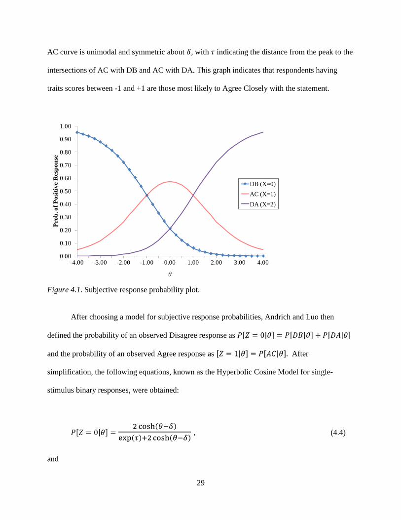
An illustrative subjective probability plot is presented in Figure 4.1 for a hypothetical
statement having 𝛿 = 0 and 𝜏 = 1. It can be seen that the DB and DA curves are monotonic and
s-shaped, like those associated with the Rasch model for dichotomous responses. In contrast, the
29
AC curve is unimodal and symmetric about 𝛿, with 𝜏 indicating the distance from the peak to the
intersections of AC with DB and AC with DA. This graph indicates that respondents having
traits scores between -1 and +1 are those most likely to Agree Closely with the statement.
Figure 4.1. Subjective response probability plot.
After choosing a model for subjective response probabilities, Andrich and Luo then
defined the probability of an observed Disagree response as 𝑃[𝑍 = 0|𝜃] = 𝑃[𝐷𝐵|𝜃] + 𝑃[𝐷𝐴|𝜃]
and the probability of an observed Agree response as [𝑍 = 1|𝜃] = 𝑃[𝐴𝐶|𝜃]. After
simplification, the following equations, known as the Hyperbolic Cosine Model for single-
stimulus binary responses, were obtained:
𝑃[𝑍 = 0|𝜃] = 2 cosh(𝜃−𝛿)
exp(𝜏)+2cosh(𝜃−𝛿) , (4.4)
and
0.00
0.10
0.20
0.30
0.40
0.50
0.60
0.70
0.80
0.90
1.00
-4.00 -3.00 -2.00 -1.00 0.00 1.00 2.00 3.00 4.00
Prob
. of P
ositi
ve R
espo
nse
θ
DB (X=0)AC (X=1)DA (X=2)
30
𝑃[𝑍 = 1|𝜃] = exp(𝜏)
exp(𝜏)+2cosh(𝜃−𝛿) . (4.5)
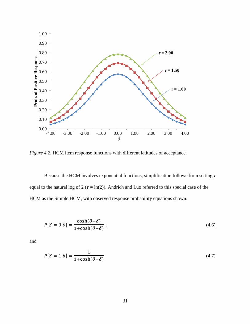
In this form, 𝜏 represents a “unit” parameter, referred to as the latitude of acceptance,
which is somewhat similar to item discrimination parameters in other IRT models (Roberts,
Rost, & Macready, 2000). The latitude of acceptance influences both the height and width of the
peak of an HCM item response function (IRF), which portrays the probability of agreeing with a
statement as a function of trait level (𝜃). The larger is 𝜏 (i.e., the wider is the latitude of
acceptance), the more likely a respondent is to agree with a statement regardless of his or her
trait level. Figure 4.2 presents three HCM IRFs with 𝛿=0 and varying 𝜏 parameters for
illustration.
A Special Case: The Simple HCM (SHCM)
Andrich and Luo (1993) discussed several options regarding the estimation of HCM
latitude of acceptance parameters. As an alternative to estimating a unique 𝜏 for every statement
in a measure, a single 𝜏 can be estimated by imposing equality constraints across statements, or 𝜏
can simply be set to a specific value, as can be done to obtain the Rasch (1960) model from
Birnbaum’s (1968) two-parameter logistic model, by setting all discrimination (a) parameters
equal to 1.
31
Figure 4.2. HCM item response functions with different latitudes of acceptance.
Because the HCM involves exponential functions, simplification follows from setting 𝜏
equal to the natural log of 2 (𝜏 = ln(2)). Andrich and Luo referred to this special case of the
HCM as the Simple HCM, with observed response probability equations shown:
𝑃[𝑍 = 0|𝜃] = cosh(𝜃−𝛿)
1+cosh(𝜃−𝛿) , (4.6)
and
𝑃[𝑍 = 1|𝜃] = 1
1+cosh(𝜃−𝛿) . (4.7)
0.00
0.10
0.20
0.30
0.40
0.50
0.60
0.70
0.80
0.90
1.00
-4.00 -3.00 -2.00 -1.00 0.00 1.00 2.00 3.00 4.00
Prob
. of P
ositi
ve R
espo
nse
θ
τ = 1.00
τ = 1.50
τ = 2.00
32
Advantages of the HCM and SHCM as a Basis for MFC Test Construction
In comparison with the Generalized Graded Unfolding Model for dichotomous responses
(GGUM; Roberts, Donoghue, & Laughlin, 2000), the HCM has a much simpler form and,
therefore, provides a more tractable basis for MFC models, such as the MUPP (Stark, 2002;
Stark et al., 2005), PICK and RANK (de la Torre et al., 2012) models, discussed in previous
chapters. This simplicity becomes more apparent when deriving first and second derivatives of
the probability equations, which are needed for computing item information and standard errors,
as well as estimating item parameters with marginal maximum likelihood techniques. Moreover,
even with MCMC estimation methods that do not require derivatives for parameter estimation,
this simplicity may have practical benefits in terms of computing time and the sample sizes
required for item calibration.
Other than the few examples provided by Andrich and coauthors when deriving the
model and examining parameter recovery with the joint maximum likelihood estimation method
implemented in the RUMMFOLD program (Andrich, & Luo, 1996), there have been very few
published applications of the HCM and its variations to date. A literature search revealed just
two: Touloumtzoglou (1999) who used the model to assess attitudes towards the visual arts, and
McGrane (2009) who evaluated measures of ambivalence. As noted by Stark, Chernyshenko,
and Lee (2000), who explored the fit of the HCM to personality scales of the Sixteen Personality
Factor Questionnaire (5th edition; Cattell & Cattell, 1995), the item parameter estimates provided
by RUMMFOLD were on a different scale than the other models. Rather than identifying the
metric by assuming the trait distribution has a mean of zero and a variance of 1, as is common
33
with other IRT software, RUMMFOLD’s joint maximum likelihood estimation procedure
identifies the metric by constraining location parameters to sum to zero, ∑ 𝛿𝑖𝐼𝑖=1 = 0,
making it difficult to evaluate fit with external programs that conveniently assume a standard
normal trait distribution for fit plots and chi-squares computations (e.g., Drasgow et al., 1995;
Stark, 2004; Tay, Ali, Drasgow, & Williams, 2011). This issue is illustrated clearly in Andrich
(1996), which reported location parameter estimates ranging from -9.80 to 8.47 for statements
reflecting attitudes toward capital punishment.
Summary
In summary, the HCM has several features that make it an attractive alternative to the
GGUM (Roberts, Donoghue, & Laughlin, 2000) for single-statement responses, as well as an
attractive basis for MFC tetrad applications. However, scaling issues and concerns about the
accuracy of joint maximum likelihood parameter estimation with small samples have likely
limited its use. Simulation research currently underway by Seybert and colleagues aims to
address that issue by providing MCMC estimation algorithms that yield parameter estimates on
the familiar standard normal scale. Doing so should facilitate interpretation and evaluations of fit
relative to competing models, via programs, such as MODFIT (Stark, 2004). Because this
ongoing research has shown that HCM and SHCM parameters can be recovered accurately for
samples varying widely in size and tests varying in length, the HCM and SHCM were chosen as
the basis for developing new models for MFC PICK and RANK, which are described in
upcoming chapters.
34
CHAPTER 5:
HYPERBOLIC COSINE MODELS FOR MULTIDIMENSIONAL FORCED CHOICE
RESPONSES:
INTRODUCING THE HCM-PICK AND HCM-RANK MODELS
As discussed in Chapter 3, the PICK model provides a general way to compute the
probability of a most like choice from a set of M alternatives, and the RANK model provides a
general way to decompose a set of ranks among M alternatives into a series of M-1 independent
PICK applications, having probabilities that multiply to give the probability of a particular rank
ordering. As a basis for estimating parameters for these models in connection with MFC tetrads,
de la Torre et al. (2012) chose the Generalized Graded Unfolding Model (GGUM; Roberts,
Donoghue, & Laughlin, 2000) for computing the necessary PICK statement agreement
probabilities.
In Chapter 4, it was suggested that Andrich and Luo’s (1993) Hyperbolic Cosine Model
(HCM) and Simple Hyperbolic Cosine Model (SHCM) provide simpler alternatives to the
GGUM for characterizing unidimensional single-statement responses. However, questions
concerning the metric of HCM statement parameter estimates and their accuracy in small
samples have limited use. It was also stated that ongoing simulation research has shown that
newly developed Markov Chain Monte Carlo (MCMC) estimation methods can provide accurate
and readily interpretable parameter HCM parameter estimates with samples of various sizes and
scales of various lengths (Seybert, Stark, & Chun, manuscript in preparation). Thus, the HCM
and SHCM can now be considered viable alternatives for computing PICK statement agreement
35
probabilities. With this idea in mind, HCM-based versions of the PICK and RANK models and
MCMC parameter estimation procedures for MFC were developed. The models and estimation
methods are summarized in the following sections of this chapter, with intermediate steps in
these derivations provided in Appendix A.
The HCM-PICK: A Hyperbolic Cosine Model for Most Like Responses
A Formulation for Tetrads
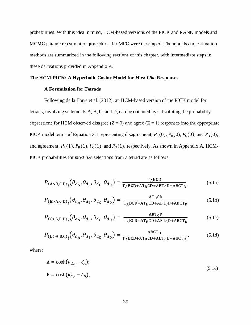
Following de la Torre et al. (2012), an HCM-based version of the PICK model for
tetrads, involving statements A, B, C, and D, can be obtained by substituting the probability
expressions for HCM observed disagree (Z = 0) and agree (Z = 1) responses into the appropriate
PICK model terms of Equation 3.1 representing disagreement, 𝑃A(0), 𝑃B(0), 𝑃C(0), and 𝑃D(0),
and agreement, 𝑃A(1), 𝑃B(1), 𝑃C(1), and 𝑃D(1), respectively. As shown in Appendix A, HCM-
PICK probabilities for most like selections from a tetrad are as follows:
𝑃(A>B,C,D)𝑖�𝜃𝑑A ,𝜃𝑑B ,𝜃𝑑C ,𝜃𝑑D� = TABCD
TABCD+ATBCD+ABTCD+ABCTD (5.1a)
𝑃(B>A,C,D)𝑖�𝜃𝑑A ,𝜃𝑑B ,𝜃𝑑C ,𝜃𝑑D� = ATBCD
TABCD+ATBCD+ABTCD+ABCTD (5.1b)
𝑃(C>A,B,D)𝑖�𝜃𝑑A ,𝜃𝑑B ,𝜃𝑑C ,𝜃𝑑D� = ABTCD
TABCD+ATBCD+ABTCD+ABCTD (5.1c)
𝑃(D>A,B,C)𝑖�𝜃𝑑A ,𝜃𝑑B ,𝜃𝑑C ,𝜃𝑑D� = ABCTD
TABCD+ATBCD+ABTCD+ABCTD , (5.1d)
where:
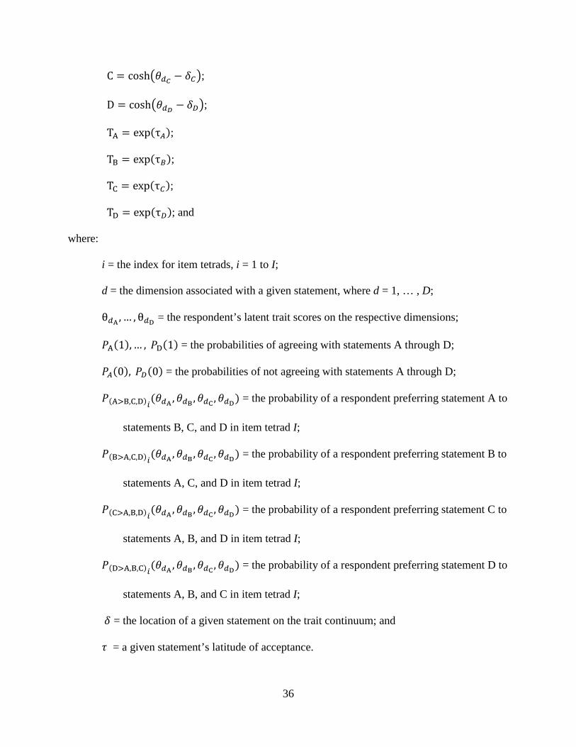
A = cosh�𝜃𝑑𝐴 − 𝛿𝐴�;
B = cosh�𝜃𝑑𝐵 − 𝛿𝐵�; (5.1e)
36
C = cosh�𝜃𝑑𝐶 − 𝛿𝐶�;
D = cosh�𝜃𝑑𝐷 − 𝛿𝐷�;
TA = exp(τ𝐴);
TB = exp(τ𝐵);
TC = exp(τ𝐶);
TD = exp(τ𝐷); and
where:
i = the index for item tetrads, i = 1 to I;
d = the dimension associated with a given statement, where d = 1, … , D;
θ𝑑A , … , θ𝑑D = the respondent’s latent trait scores on the respective dimensions;
𝑃A(1), … , 𝑃D(1) = the probabilities of agreeing with statements A through D;
𝑃𝐴(0), 𝑃𝐷(0) = the probabilities of not agreeing with statements A through D;
𝑃(A>B,C,D)𝑖(𝜃𝑑A ,𝜃𝑑B ,𝜃𝑑C ,𝜃𝑑D) = the probability of a respondent preferring statement A to
statements B, C, and D in item tetrad I;
𝑃(B>A,C,D)𝑖(𝜃𝑑A ,𝜃𝑑B ,𝜃𝑑C ,𝜃𝑑D) = the probability of a respondent preferring statement B to
statements A, C, and D in item tetrad I;
𝑃(C>A,B,D)𝑖(𝜃𝑑A ,𝜃𝑑B ,𝜃𝑑C ,𝜃𝑑D) = the probability of a respondent preferring statement C to
statements A, B, and D in item tetrad I;
𝑃(D>A,B,C)𝑖(𝜃𝑑A ,𝜃𝑑B ,𝜃𝑑C ,𝜃𝑑D) = the probability of a respondent preferring statement D to
statements A, B, and C in item tetrad I;
𝛿 = the location of a given statement on the trait continuum; and
𝜏 = a given statement’s latitude of acceptance.
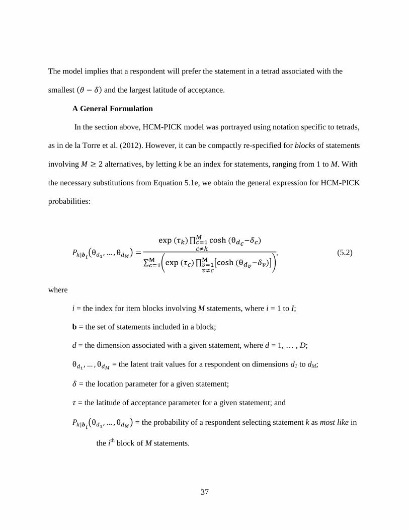
37
The model implies that a respondent will prefer the statement in a tetrad associated with the
smallest (𝜃 − 𝛿) and the largest latitude of acceptance.
A General Formulation
In the section above, HCM-PICK model was portrayed using notation specific to tetrads,
as in de la Torre et al. (2012). However, it can be compactly re-specified for blocks of statements
involving 𝑀 ≥ 2 alternatives, by letting k be an index for statements, ranging from 1 to M. With
the necessary substitutions from Equation 5.1e, we obtain the general expression for HCM-PICK
probabilities:
𝑃𝑘|𝒃𝑖�θ𝑑1 , … , θ𝑑𝑀� =
exp (𝜏𝑘)∏ cosh (θ𝑑𝑐−𝛿𝑐)𝑀𝑐=1𝑐≠𝑘
∑ �exp (𝜏𝑐)∏ �cosh (θ𝑑𝑣−𝛿𝑣)�M𝑣=1𝑣≠𝑐
�M𝑐=1
, (5.2)
where
i = the index for item blocks involving M statements, where i = 1 to I;
b = the set of statements included in a block;
d = the dimension associated with a given statement, where d = 1, … , D;
θ𝑑1 , … , θ𝑑𝑀 = the latent trait values for a respondent on dimensions d1 to dM;
𝛿 = the location parameter for a given statement;
𝜏 = the latitude of acceptance parameter for a given statement; and
𝑃𝑘|𝒃𝑖�θ𝑑1 , … , θ𝑑𝑀� = the probability of a respondent selecting statement k as most like in
the ith block of M statements.
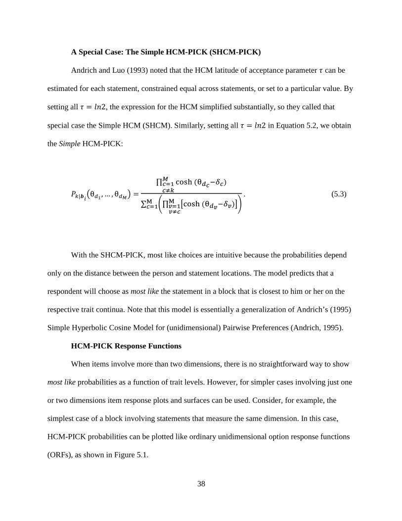
38
A Special Case: The Simple HCM-PICK (SHCM-PICK)
Andrich and Luo (1993) noted that the HCM latitude of acceptance parameter 𝜏 can be
estimated for each statement, constrained equal across statements, or set to a particular value. By
setting all 𝜏 = 𝑙𝑛2, the expression for the HCM simplified substantially, so they called that
special case the Simple HCM (SHCM). Similarly, setting all 𝜏 = 𝑙𝑛2 in Equation 5.2, we obtain
the Simple HCM-PICK:
𝑃𝑘|𝒃𝑖�θ𝑑1 , … , θ𝑑𝑀� =
∏ cosh (θ𝑑𝑐−𝛿𝑐)𝑀𝑐=1𝑐≠𝑘
∑ �∏ �cosh (θ𝑑𝑣−𝛿𝑣)�M𝑣=1𝑣≠𝑐
�M𝑐=1
. (5.3)
With the SHCM-PICK, most like choices are intuitive because the probabilities depend
only on the distance between the person and statement locations. The model predicts that a
respondent will choose as most like the statement in a block that is closest to him or her on the
respective trait continua. Note that this model is essentially a generalization of Andrich’s (1995)
Simple Hyperbolic Cosine Model for (unidimensional) Pairwise Preferences (Andrich, 1995).
HCM-PICK Response Functions
When items involve more than two dimensions, there is no straightforward way to show
most like probabilities as a function of trait levels. However, for simpler cases involving just one
or two dimensions item response plots and surfaces can be used. Consider, for example, the
simplest case of a block involving statements that measure the same dimension. In this case,
HCM-PICK probabilities can be plotted like ordinary unidimensional option response functions
(ORFs), as shown in Figure 5.1.
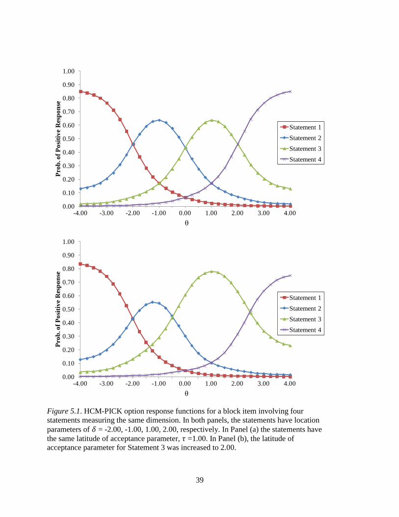
39
Figure 5.1. HCM-PICK option response functions for a block item involving four statements measuring the same dimension. In both panels, the statements have location parameters of 𝛿 = -2.00, -1.00, 1.00, 2.00, respectively. In Panel (a) the statements have the same latitude of acceptance parameter, 𝜏 =1.00. In Panel (b), the latitude of acceptance parameter for Statement 3 was increased to 2.00.
0.00
0.10
0.20
0.30
0.40
0.50
0.60
0.70
0.80
0.90
1.00
-4.00 -3.00 -2.00 -1.00 0.00 1.00 2.00 3.00 4.00
Prob
. of P
ositi
ve R
espo
nse
θ
Statement 1Statement 2Statement 3Statement 4
0.00
0.10
0.20
0.30
0.40
0.50
0.60
0.70
0.80
0.90
1.00
-4.00 -3.00 -2.00 -1.00 0.00 1.00 2.00 3.00 4.00
Prob
. of P
ositi
ve R
espo
nse
θ
Statement 1Statement 2Statement 3Statement 4
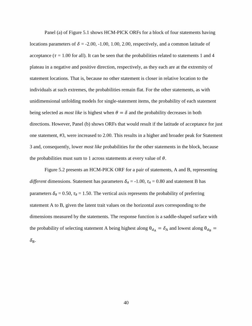
40
Panel (a) of Figure 5.1 shows HCM-PICK ORFs for a block of four statements having
locations parameters of 𝛿 = -2.00, -1.00, 1.00, 2.00, respectively, and a common latitude of
acceptance (𝜏 = 1.00 for all). It can be seen that the probabilities related to statements 1 and 4
plateau in a negative and positive direction, respectively, as they each are at the extremity of
statement locations. That is, because no other statement is closer in relative location to the
individuals at such extremes, the probabilities remain flat. For the other statements, as with
unidimensional unfolding models for single-statement items, the probability of each statement
being selected as most like is highest when 𝜃 = 𝛿 and the probability decreases in both
directions. However, Panel (b) shows ORFs that would result if the latitude of acceptance for just
one statement, #3, were increased to 2.00. This results in a higher and broader peak for Statement
3 and, consequently, lower most like probabilities for the other statements in the block, because
the probabilities must sum to 1 across statements at every value of 𝜃.
Figure 5.2 presents an HCM-PICK ORF for a pair of statements, A and B, representing
different dimensions. Statement has parameters δA = -1.00, τA = 0.80 and statement B has
parameters δB = 0.50, τB = 1.50. The vertical axis represents the probability of preferring
statement A to B, given the latent trait values on the horizontal axes corresponding to the
dimensions measured by the statements. The response function is a saddle-shaped surface with
the probability of selecting statement A being highest along θ𝑑A = 𝛿A and lowest along θ𝑑B =
𝛿B.
41
Figure 5.2. HCM-PICK option response function selecting statement A (δ = -1.00, τ = 0.80) over statement B (δ = 0.50, τ = 1.50) in a 2-dimensional pair. The HCM-RANK: A Hyperbolic Cosine Model for Rank Order Responses
de la Torre et al. (2012) showed how one could obtain the probability of rank responses
by successive applications of the PICK model, using the GGUM as the basis for computing
statement agreement probabilities. The same process can therefore be used to calculate the
probability of a set of ranks based on the HCM.
Returning to the Chapter 3 example of an item tetrad for which a respondent indicates the
following pattern of preferences, A>D>C>B, where > means “preferred,” three HCM-PICK
probabilities can be calculated:
1. 𝑃(A>B,C,D) = probability of selecting A as most like from the block of four statements;
2. 𝑃(D>B,C)) = probability of selecting D as most like from the remaining three; and
3. 𝑃(B>C) = probability of selecting B as most like from the remaining two.
-4-3
-2-1
01
23
4
0.00
0.20
0.40
0.60
0.80
1.00
-4.00-3.00
-2.00-1.00
0.001.00
2.003.00
4.00

42
The probability of the ranking A>D>B>C is equal to the product of the three HCM-PICK
probabilities: 𝑃(A>D>B>C)𝑖�𝜃𝑑A ,𝜃𝑑B ,𝜃𝑑C ,𝜃𝑑D� = 𝑃(A>B,C,D)𝑃(D>B,C)𝑃(B>C).
To provide a general expression for the probability of rank responses based on successive
applications of the HCM-PICK model, as illustrated above, it is convenient to represent a set of
ranks as an (Mx1) column vector �⃗�, with the rank of the least preferred alternative assigned to
row 1, and the rank of the most preferred alternative assigned to row M. For example, the
ranking A>D>B>C for the M=4, block above would be represented by the column vector
�⃗�𝑀𝑥1 = �
CBDA
�. This organization allows for the derivation of a single expression for the HCM-
RANK, utilizing a product operator to step through successive HCM-PICK probabilities to
calculate the probability of a set of ranks. Using this notation, the following general formulation,
referred to as the HCM-RANK model results:
𝑃𝐛𝚤����⃗ (𝛉) = ∏ exp (𝜏𝑘)∏ cosh (θ𝑑𝑐−𝛿𝑐)𝑘−1𝑐=1
∑ �exp (𝜏𝑐)∏ �cosh (θ𝑑𝑣−𝛿𝑣)�k𝑣=1𝑣≠𝑐
�k𝑐=1
𝑀𝑘=2 , (5.4)
where:
i = the index for item blocks involving M statements, where i = 1 to I;
�⃗�𝑖 = a vector of assigned ranks for the ith block, arranged from least preferred (1) to most
preferred (M);
d = the dimension associated with a given statement, where d = 1, … , D;
𝛉 = a vector of latent trait values for a respondent on dimensions d1 to dM;
𝛿 = the location of a statement on the trait continuum;
43
𝜏 = the latitude of acceptance parameter for a statement; and
𝑃𝐛𝚤����⃗ (𝛉) = the probability of a ranking of M statements by a respondent with trait scores 𝛉.
As was the case with the HCM, setting the latitude of acceptance to 𝜏 = 𝑙𝑛 (2) in Equation 5.4,
leads to the following simplified model known as the Simple HCM-PICK (SHCM-PICK).
𝑃𝐛𝚤����⃗ (𝛉) = ∏∏ cosh (θ𝑑𝑐−𝛿𝑐)𝑘−1𝑐=1
∑ �∏ �cosh (θ𝑑𝑣−𝛿𝑣)�k𝑣=1𝑣≠𝑐
�k𝑐=1
𝑀𝑘=2 , (5.5)
Summary and Preview
In this chapter, new models were developed to characterize most like and rank responses
to multidimensional block items. The new HCM-PICK and HCM-RANK models and their
special cases, the SHCM-PICK and SHCM-RANK models, provide a basis for constructing and
scoring better multidimensional forced choice assessments, such as situational judgment tests
(SJTs), which consist of scenarios followed by blocks of statements representing different
response styles. In an SJT, examinees are asked to consider each scenario and indicate what they
should/would do by choosing the best/most likely option or by ranking options from best/most
likely to worst/least likely. The equations for item response functions and item information
functions presented above provide the necessary foundations for estimating item and person
parameters directly from examinee responses, as well as for improving item quality, building
parallel test forms, equating, and detecting differential functioning.
Parameter estimation for the most general model described here, namely the HCM-
RANK model, is the focus of upcoming chapters. Chapter 6 provides a brief overview of Markov

44
chain Monte Carlo (MCMC) estimation and describes an algorithm for estimating HCM-RANK
model parameters. Following this, a series of simulation and empirical studies are provided to
investigate the efficacy of the HCM-RANK and SHCM-RANK models.
45
CHAPTER 6:
HCM-RANK Model Item and Person Parameter Estimation
Many methods have been developed and tested for estimating item and person parameters
associated with item response theory models. Historically, joint maximum likelihood (JML) and
marginal maximum likelihood (MML) methods are among the most popular (Baker & Kim,
2004). In JML estimation, item and person parameters are estimated through a sequential,
iterative process, which begins with provisional estimates of item parameters. These provisional
item parameters are used to estimate trait scores, which are then used to improve the provisional
item parameter estimates, and this back and forth process continues until stable item and person
estimates are obtained. The main concern with JML estimation is that item parameter estimates
do not necessarily improve with sample size (i.e., they are not consistent), because as sample size
increases, so does the number of person parameters that need to be estimated (Hulin, Drasgow, &
Parsons, 1983).
Marginal maximum likelihood (MML) estimation methods address this issue by
eliminating the dependency of the item parameter estimates on the trait score distribution. In a
seminal paper, Bock and Aitkin (1981) illustrated how consistent item parameter estimates could
be obtained via an expectation-maximization (EM) algorithm. Person parameter estimates can
then be estimated in a separate run using one of many available methods.
An unfortunate drawback of both of JML and MML methods is that estimation involves a
maximization process that requires first and second derivatives of a likelihood function with
respect to model parameters. Second derivatives, in particular, can become difficult to derive as
46
model complexity increases. Consequently, methods that do not require explicit expressions for
these derivatives have many practical advantages.
Markov chain Monte Carlo (MCMC) methods provide a way to estimate item and person
parameters without complicated derivatives (Patz & Junker, 1999a). Instead, MCMC methods
estimate model parameters by computing the means and standard deviations of posterior
distributions obtained by repeated sampling. Parameters to be estimated are assumed to have
prior distributions, which may be chosen on empirical or practical grounds. Provisional
parameter values are specified, posterior values are calculated using the likelihood of the
response data and the provisional values, and the process is repeated for thousands of cycles. On
each cycle, a decision is made to accept or reject a provisional value in favor of a current one,
depending on the likelihood of the data under the two alternatives. If a provisional value makes
the observed data more likely, then it is accepted; otherwise it is rejected probabilistically. The
result is a Markov chain, in which the parameter values at any point depend only on the previous
cycle. Given enough cycles, this chain theoretically will converge on a stationary distribution
that is the desired posterior, regardless of the choice of priors. However, because the early states
in the chain clearly depend on the priors, the first few hundred or thousand cycles are typically
discarded (i.e., “burn in”) when computing the posterior means and standard deviations that
serve as the final item and person parameter estimates.
Note that because MCMC methods estimate item and person parameters simultaneously,
it is akin to joint maximum likelihood (JML) estimation, which may raise questions about
consistency of the estimates; e.g., do the item parameter estimates improve with sample size?
Most research suggests that consistency is not a big concern. But if it is, one solution is to
analyze the data twice, treating the item or person parameters as fixed at the values obtained in
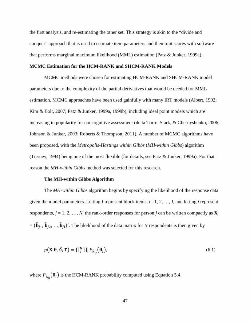
47
the first analysis, and re-estimating the other set. This strategy is akin to the “divide and
conquer” approach that is used to estimate item parameters and then trait scores with software
that performs marginal maximum likelihood (MML) estimation (Patz & Junker, 1999a).
MCMC Estimation for the HCM-RANK and SHCM-RANK Models
MCMC methods were chosen for estimating HCM-RANK and SHCM-RANK model
parameters due to the complexity of the partial derivatives that would be needed for MML
estimation. MCMC approaches have been used gainfully with many IRT models (Albert, 1992;
Kim & Bolt, 2007; Patz & Junker, 1999a, 1999b), including ideal point models which are
increasing in popularity for noncognitive assessment (de la Torre, Stark, & Chernyshenko, 2006;
Johnson & Junker, 2003; Roberts & Thompson, 2011). A number of MCMC algorithms have
been proposed, with the Metropolis-Hastings within Gibbs (MH-within Gibbs) algorithm
(Tierney, 1994) being one of the most flexible (for details, see Patz & Junker, 1999a). For that
reason the MH-within Gibbs method was selected for this research.
The MH-within Gibbs Algorithm
The MH-within Gibbs algorithm begins by specifying the likelihood of the response data
given the model parameters. Letting I represent block items, i =1, 2, …, I, and letting j represent
respondents, j = 1, 2, …, N, the rank-order responses for person j can be written compactly as Xj
= {�⃗�𝑗1, �⃗�𝑗2, …,�⃗�𝑗I}´. The likelihood of the data matrix for N respondents is then given by
𝑝�𝐗|𝛉,𝛿,𝜏� = ∏ ∏ 𝑃�⃗�𝒊𝒋�𝛉𝑗�I𝑖
N𝑗 , (6.1)
where 𝑃�⃗�𝒊𝒋�𝛉𝑗� is the HCM-RANK probability computed using Equation 5.4.
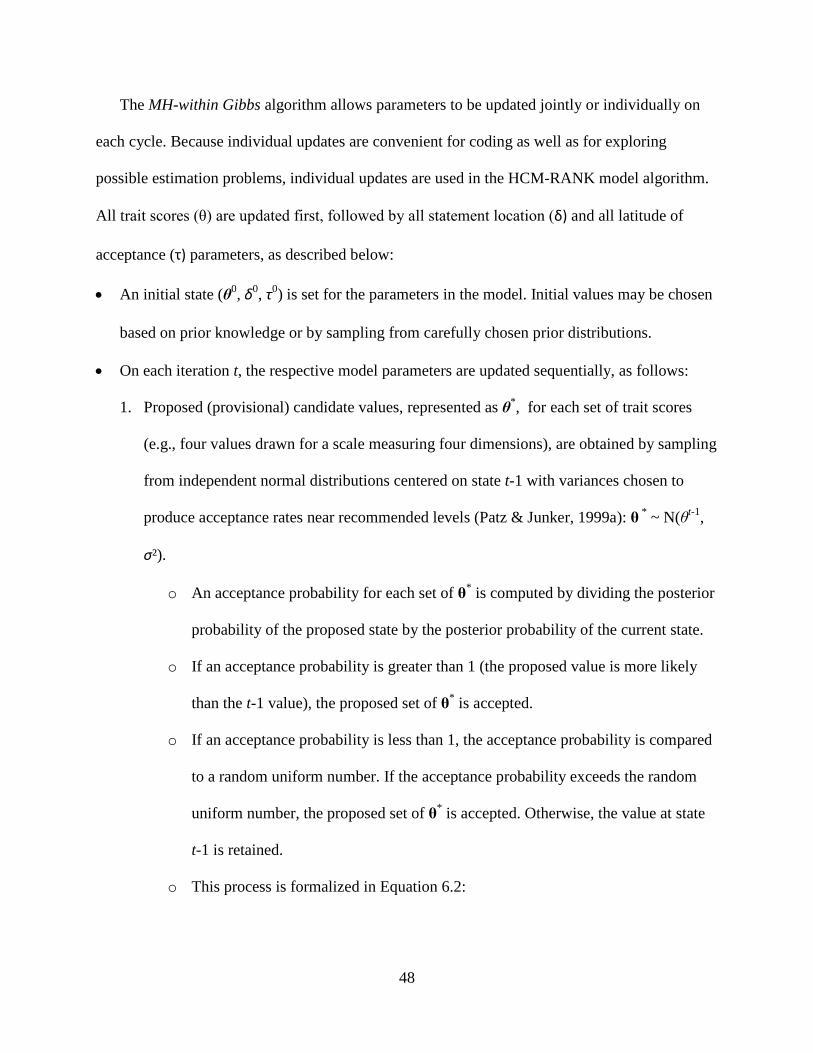
48
The MH-within Gibbs algorithm allows parameters to be updated jointly or individually on
each cycle. Because individual updates are convenient for coding as well as for exploring
possible estimation problems, individual updates are used in the HCM-RANK model algorithm.
All trait scores (θ) are updated first, followed by all statement location (δ) and all latitude of
acceptance (τ) parameters, as described below:
• An initial state (θ0, δ0, τ0) is set for the parameters in the model. Initial values may be chosen
based on prior knowledge or by sampling from carefully chosen prior distributions.
• On each iteration t, the respective model parameters are updated sequentially, as follows:
1. Proposed (provisional) candidate values, represented as θ*, for each set of trait scores
(e.g., four values drawn for a scale measuring four dimensions), are obtained by sampling
from independent normal distributions centered on state t-1 with variances chosen to
produce acceptance rates near recommended levels (Patz & Junker, 1999a): θ * ~ N(θt-1,
σ²).
o An acceptance probability for each set of θ* is computed by dividing the posterior
probability of the proposed state by the posterior probability of the current state.
o If an acceptance probability is greater than 1 (the proposed value is more likely
than the t-1 value), the proposed set of θ* is accepted.
o If an acceptance probability is less than 1, the acceptance probability is compared
to a random uniform number. If the acceptance probability exceeds the random
uniform number, the proposed set of θ* is accepted. Otherwise, the value at state
t-1 is retained.
o This process is formalized in Equation 6.2:

49
( )( )
=−−−−
−−− 1,
),,|(),,|(min),( )1t()1t()1t()1t(
*)1t()1t(**)1t(
pPpPpθθXθθXθθ
τδτδ
. (6.2)
2. Proposed candidate values for statement location parameters δ* are sampled from
independent normal distributions centered on state t-1 with appropriately chosen
variances: δ * ~ N(δt-1, σ²).
o An acceptance probability for each δ* is computed by dividing the posterior
probability of the proposed state by the posterior probability of the current state.
o The proposed states are accepted or rejected probabilistically by comparing the
acceptance probabilities to random uniform numbers, as shown in Equation 6.3:
, (6.3)
3. Proposed candidate values for latitude of acceptance parameters, τ*, are sampled from
independent normal distributions centered on state t-1 with appropriately chosen
variances: τ* ~ N(τ t-1, σ²).
o An acceptance probability for each τ * is computed by dividing the posterior
probability of the proposed state by the posterior probability of the current state.
o The proposed states are accepted or rejected probabilistically by comparing the
acceptance probabilities to random uniform numbers, as shown in Equation 6.4:
( )( )
* ( 1) *( 1) *
( 1) ( 1) ( 1)
P( | , , )pp( , ) min , 1
P( | , , )p
t tt
t t t t
δ τ δδ δ
δ τ δ
−−
− − −
=
Xθ
Xθ
50
, (6.4)
• This process continues, saving the item and person parameter values on each cycle, until a
designated maximum number of cycles is reached. The values obtained before stationarity is
believed to occur are typically discarded. Then means, variances, and covariances of the item
and person parameters are computed using the remaining cycles to get the desired parameter
estimates, standard errors, and covariance information.
Note that to estimate item and person parameters for the SHCM-RANK model, only
slight changes to this algorithm are needed. Since the SHCM-RANK model has no latitude of
acceptance parameters, Step 3 can be omitted. In addition, if statement location parameters are
known in advance, as might be the case when using SME judgments for scoring, location
parameters can be fixed on every cycle, leaving just Step 1 to be executed.
These estimation strategies have been implemented in the Ox (Doornik, 2009)
programming language to conduct the studies in this dissertation. Effective prior distributions for
the θ, δ, and τ parameters were determined at the simulation stage and proposal variances were
set for each specific condition following the recommendations laid out by Patz and Junker
(1999a).
( )( )
* *( 1) *
( 1) ( 1)
P( | , , )pp( , ) min , 1
P( | , , )p
tt
t t t t
tδ τ ττ τ
δ τ τ−
− −
=
Xθ
Xθ
51
CHAPTER 7:
STUDY 1: A MONTE CARLO SIMULATION TO ASSESS THE EFFICACY OF
HCM-RANK PARAMETER ESTIMATION METHODS
This chapter describes a Monte Carlo study to answer several key questions about HCM-
RANK and SHCM-RANK model parameter estimation. First and foremost, the simulation
examines the accuracy of MCMC parameter recovery from rank responses, generated under
controlled conditions, using statement parameters obtained from real data to increase external
validity. Of interest is how closely the parameter estimates obtained directly from the rank data
match the generating (true) values in each experimental condition, as indicated by correlations
between the estimated and true parameters, bias, and root mean square error statistics. This
simulation also compares the results of this direct estimation process to those obtained through a
two-stage process involving statement precalibration (Stark, 2002; see Chapter 2). In the two-
stage process, statements composing MFC items are administered individually to a sample of
respondents and calibrated, one dimension at a time, using a unidimensional model (i.e.,
precalibration). The resulting statement parameter estimates are then used to score the choice or
rank responses to the MFC items. Because the direct and two-stage processes have distinct
advantages and disadvantages, the findings of this comparison could have important implications
for practice.

52
Study Design
To examine HCM-RANK and SHCM-RANK parameter estimation, 20-item-tetrad MFC
tests were constructed and administered to simulated examinees in 16 conditions associated with
four fully-crossed independent variables:
1) Sample size:
a) N = 250; and
b) N = 500.
2) Dimensionality of MFC assessment:
a) 4 dimensions; and
b) 8 dimensions.
3) Estimation strategy:
a) Direct: Estimate item and person parameters directly (simultaneously) from MFC
rank responses; and
b) Two-stage: Precalibrate statements using a unidimensional model; then score
MFC rank responses using those statement parameter estimates.
4) Model:
a) HCM: In direct conditions, use the HCM-RANK model to simultaneously
estimate item and person parameters from MFC rank responses. In two-stage
conditions, precalibrate statements using the HCM; then score MFC rank
responses via the HCM-RANK; and
b) SHCM: In direct conditions, use the SHCM-RANK model to simultaneously
estimate item and person parameters from MFC rank responses. In two-stage

53
conditions, precalibrate statements using the SHCM; then score MFC rank
responses via the SHCM-RANK.
As run times for a single replication for direct conditions ranged from 6 to 12 hours, 30
replications were conducted in each condition.
Constructing MFC Measures for the Simulation
Statement Parameter Data
To increase realism, the two MFC tests needed for this simulation were constructed by
following procedures used in organizations to develop measures aimed at reducing socially
desirable responding. Rather than sampling the generating item parameters and social desirability
ratings from idealized distributions for MFC test construction (e.g., Brown & Maydeu-Olivares,
2011; de la Torre et al., 2012), the generating item parameters for this study were obtained by
calibrating real single-statement personality data that were collected as part of a larger previous
investigation (Loo, manuscript in preparation). A sample of 302 respondents indicated their level
of agreement on a 1 (Strongly Disagree) to 4 (Strongly Agree) scale with 160 personality
statements (see Appendix B) measuring conscientiousness, emotional stability, openness to
experience, and extraversion. These statements were a combination of items obtained from the
International Personality Item Pool (IPIP; Goldberg et al., 2006) and others written by two
experts familiar with the constructs. To obtain statement parameters, first these data were
dichotomized by recoding the Strongly Disagree and Disagree responses as 0s and the Strongly
Agree and Agree responses as 1s. Second, HCM (Andrich & Luo, 1993) item parameters were
estimated separately for the statements measuring each dimension, using MCMC software
developed in an ongoing study by Seybert et al. (manuscript in preparation). Next, model-data fit
was examined using fit plots and chi-square statistics (Drasgow et al., 1995) via the MODFIT 4.0
54
computer program (Stark, 2013). Statements exhibiting poor psychometric properties or poor fit
statistics were eliminated from the pool available for MFC test construction.
Finally, the 142 statements surviving this psychometric screening were administered to
75 new respondents using the same four-point scale (1=Strongly Disagree to 4 =Strongly Agree)
for the purpose of collecting social desirability ratings. Rather than asking respondents to judge
how desirable a statement is (e.g., Heggestad et al., 2006), respondents were simply be asked to
answer in a way that presents themselves in a favorable light, as was done in the Assessment of
Individual Motivation research by White and Young (1998). The mean score for each statement
served as an indicator of its desirability.
Test Design
Tables 7.1 and 7.2 present high-level design specifications for the 4-D and 8-D MFC tests
that were used for test construction with this simulation. In each table, column 1 indicates the
tetrad number and columns 2 through 5 indicate the dimensions represented by the first, second,
third, and fourth statements. As can be seen in Table 7.1, the 4-D test has a simple design. Each
tetrad involves a statement representing a different dimension with the first statement always
representing dimension 1, the second statement measuring dimension 2, the third statement
measuring dimension 3, and the fourth statement measuring dimension 4. For the 8-D MFC test,
the number of possible combinations of four dimensions (70) greatly exceeds the desired number
of tetrads (20). To address this, a blueprint was designed to balance the number of times
dimensions appeared with one another within a tetrad. This led to a diverse grouping of
dimensions across tetrads, as can be seen in Table 7.2.
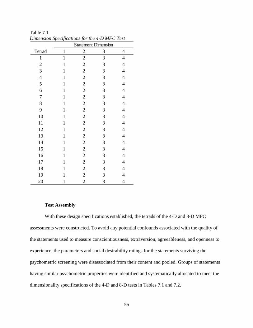
55
Table 7.1 Dimension Specifications for the 4-D MFC Test
Test Assembly
With these design specifications established, the tetrads of the 4-D and 8-D MFC
assessments were constructed. To avoid any potential confounds associated with the quality of
the statements used to measure conscientiousness, extraversion, agreeableness, and openness to
experience, the parameters and social desirability ratings for the statements surviving the
psychometric screening were disassociated from their content and pooled. Groups of statements
having similar psychometric properties were identified and systematically allocated to meet the
dimensionality specifications of the 4-D and 8-D tests in Tables 7.1 and 7.2.
Tetrad 1 2 3 41 1 2 3 42 1 2 3 43 1 2 3 44 1 2 3 45 1 2 3 46 1 2 3 47 1 2 3 48 1 2 3 49 1 2 3 4
10 1 2 3 411 1 2 3 412 1 2 3 413 1 2 3 414 1 2 3 415 1 2 3 416 1 2 3 417 1 2 3 418 1 2 3 419 1 2 3 420 1 2 3 4
Statement Dimension
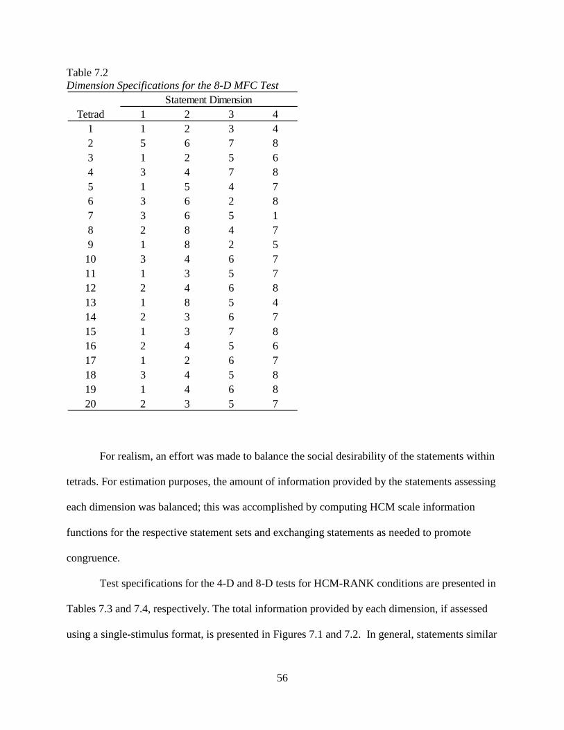
56
Table 7.2 Dimension Specifications for the 8-D MFC Test
For realism, an effort was made to balance the social desirability of the statements within
tetrads. For estimation purposes, the amount of information provided by the statements assessing
each dimension was balanced; this was accomplished by computing HCM scale information
functions for the respective statement sets and exchanging statements as needed to promote
congruence.
Test specifications for the 4-D and 8-D tests for HCM-RANK conditions are presented in
Tables 7.3 and 7.4, respectively. The total information provided by each dimension, if assessed
using a single-stimulus format, is presented in Figures 7.1 and 7.2. In general, statements similar
Tetrad 1 2 3 41 1 2 3 42 5 6 7 83 1 2 5 64 3 4 7 85 1 5 4 76 3 6 2 87 3 6 5 18 2 8 4 79 1 8 2 5
10 3 4 6 711 1 3 5 712 2 4 6 813 1 8 5 414 2 3 6 715 1 3 7 816 2 4 5 617 1 2 6 718 3 4 5 819 1 4 6 820 2 3 5 7
Statement Dimension
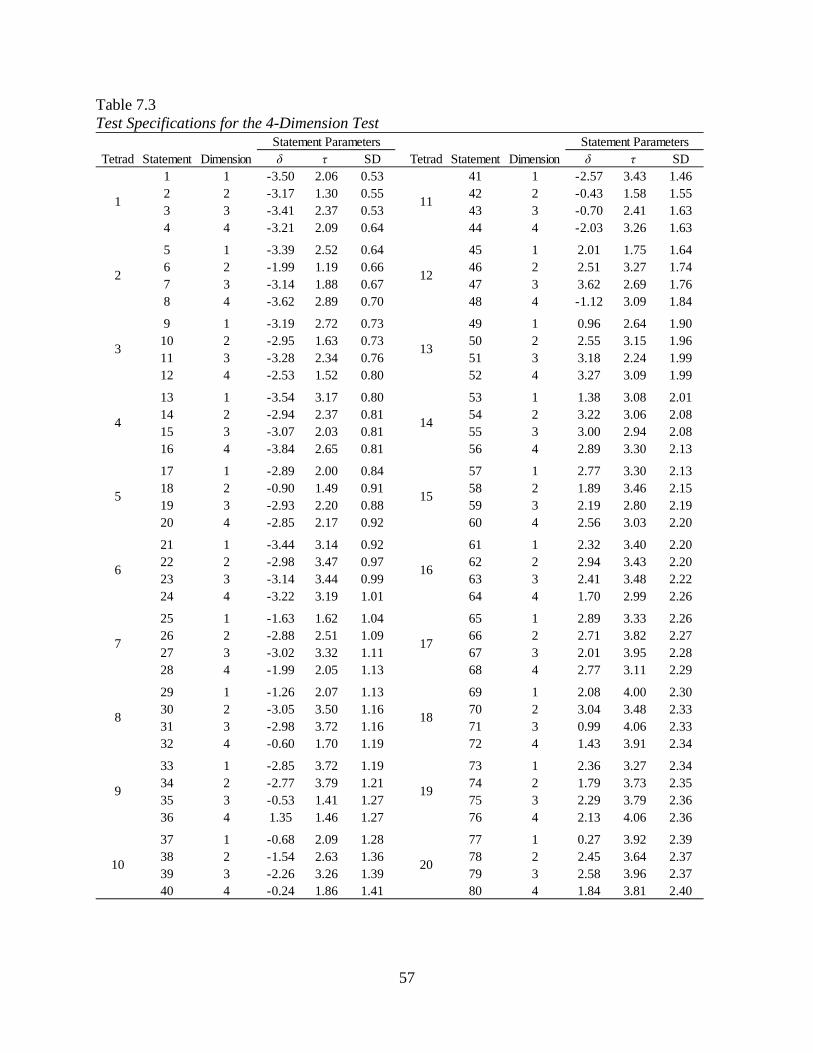
57
Table 7.3 Test Specifications for the 4-Dimension Test
Tetrad Statement Dimension δ τ SD Tetrad Statement Dimension δ τ SD1 1 -3.50 2.06 0.53 41 1 -2.57 3.43 1.462 2 -3.17 1.30 0.55 42 2 -0.43 1.58 1.553 3 -3.41 2.37 0.53 43 3 -0.70 2.41 1.634 4 -3.21 2.09 0.64 44 4 -2.03 3.26 1.63
5 1 -3.39 2.52 0.64 45 1 2.01 1.75 1.646 2 -1.99 1.19 0.66 46 2 2.51 3.27 1.747 3 -3.14 1.88 0.67 47 3 3.62 2.69 1.768 4 -3.62 2.89 0.70 48 4 -1.12 3.09 1.84
9 1 -3.19 2.72 0.73 49 1 0.96 2.64 1.9010 2 -2.95 1.63 0.73 50 2 2.55 3.15 1.9611 3 -3.28 2.34 0.76 51 3 3.18 2.24 1.9912 4 -2.53 1.52 0.80 52 4 3.27 3.09 1.99
13 1 -3.54 3.17 0.80 53 1 1.38 3.08 2.0114 2 -2.94 2.37 0.81 54 2 3.22 3.06 2.0815 3 -3.07 2.03 0.81 55 3 3.00 2.94 2.0816 4 -3.84 2.65 0.81 56 4 2.89 3.30 2.13
17 1 -2.89 2.00 0.84 57 1 2.77 3.30 2.1318 2 -0.90 1.49 0.91 58 2 1.89 3.46 2.1519 3 -2.93 2.20 0.88 59 3 2.19 2.80 2.1920 4 -2.85 2.17 0.92 60 4 2.56 3.03 2.20
21 1 -3.44 3.14 0.92 61 1 2.32 3.40 2.2022 2 -2.98 3.47 0.97 62 2 2.94 3.43 2.2023 3 -3.14 3.44 0.99 63 3 2.41 3.48 2.2224 4 -3.22 3.19 1.01 64 4 1.70 2.99 2.26
25 1 -1.63 1.62 1.04 65 1 2.89 3.33 2.2626 2 -2.88 2.51 1.09 66 2 2.71 3.82 2.2727 3 -3.02 3.32 1.11 67 3 2.01 3.95 2.2828 4 -1.99 2.05 1.13 68 4 2.77 3.11 2.29
29 1 -1.26 2.07 1.13 69 1 2.08 4.00 2.3030 2 -3.05 3.50 1.16 70 2 3.04 3.48 2.3331 3 -2.98 3.72 1.16 71 3 0.99 4.06 2.3332 4 -0.60 1.70 1.19 72 4 1.43 3.91 2.34
33 1 -2.85 3.72 1.19 73 1 2.36 3.27 2.3434 2 -2.77 3.79 1.21 74 2 1.79 3.73 2.3535 3 -0.53 1.41 1.27 75 3 2.29 3.79 2.3636 4 1.35 1.46 1.27 76 4 2.13 4.06 2.36
37 1 -0.68 2.09 1.28 77 1 0.27 3.92 2.3938 2 -1.54 2.63 1.36 78 2 2.45 3.64 2.3739 3 -2.26 3.26 1.39 79 3 2.58 3.96 2.3740 4 -0.24 1.86 1.41 80 4 1.84 3.81 2.40
Statement ParametersStatement Parameters
20
11
12
13
14
15
16
17
18
19
7
8
9
10
1
2
3
4
5
6
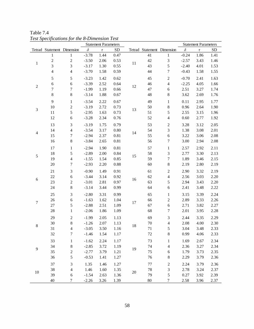
58
Table 7.4 Test Specifications for the 8-Dimension Test
Tetrad Statement Dimension δ τ SD Tetrad Statement Dimension δ τ SD1 1 -3.78 1.44 0.47 41 1 -0.24 1.86 1.412 2 -3.50 2.06 0.53 42 3 -2.57 3.43 1.463 3 -3.17 1.30 0.55 43 5 -2.40 4.01 1.534 4 -3.70 1.58 0.59 44 7 -0.43 1.58 1.55
5 5 -3.23 1.42 0.62 45 2 -0.70 2.41 1.636 6 -3.39 2.52 0.64 46 4 -2.25 4.05 1.667 7 -1.99 1.19 0.66 47 6 2.51 3.27 1.748 8 -3.14 1.88 0.67 48 8 3.62 2.69 1.76
9 1 -3.54 2.22 0.67 49 1 0.11 2.95 1.7710 2 -3.19 2.72 0.73 50 8 0.96 2.64 1.9011 5 -2.95 1.63 0.73 51 5 2.55 3.15 1.9612 6 -3.28 2.34 0.76 52 4 0.60 2.77 1.92
13 3 -3.19 1.75 0.79 53 2 3.28 3.12 2.0514 4 -3.54 3.17 0.80 54 3 1.38 3.08 2.0115 7 -2.94 2.37 0.81 55 6 3.22 3.06 2.0816 8 -3.84 2.65 0.81 56 7 3.00 2.94 2.08
17 1 -2.94 1.90 0.81 57 1 2.57 2.92 2.1118 5 -2.89 2.00 0.84 58 3 2.77 3.30 2.1319 4 -1.55 1.54 0.85 59 7 1.89 3.46 2.1520 7 -2.93 2.20 0.88 60 8 2.19 2.80 2.19
21 3 -0.90 1.49 0.91 61 2 2.90 3.32 2.1922 6 -3.44 3.14 0.92 62 4 2.56 3.03 2.2023 2 -3.01 2.81 0.97 63 5 2.94 3.43 2.2024 8 -3.14 3.44 0.99 64 6 2.41 3.48 2.22
25 3 -2.80 3.31 0.99 65 1 3.15 3.39 2.2426 6 -1.63 1.62 1.04 66 2 2.89 3.33 2.2627 5 -2.88 2.51 1.09 67 6 2.71 3.82 2.2728 1 -2.06 1.86 1.09 68 7 2.01 3.95 2.28
29 2 -1.99 2.05 1.13 69 3 2.44 3.35 2.2930 8 -1.26 2.07 1.13 70 4 2.08 4.00 2.3031 4 -3.05 3.50 1.16 71 5 3.04 3.48 2.3332 7 -1.46 1.54 1.17 72 8 0.99 4.06 2.33
33 1 -1.62 2.24 1.17 73 1 1.69 2.67 2.3434 8 -2.85 3.72 1.19 74 4 2.36 3.27 2.3435 2 -2.77 3.79 1.21 75 6 1.79 3.73 2.3536 5 -0.53 1.41 1.27 76 8 2.29 3.79 2.36
37 3 1.35 1.46 1.27 77 2 2.24 3.79 2.3638 4 1.46 1.60 1.35 78 3 2.78 3.24 2.3739 6 -1.54 2.63 1.36 79 5 0.27 3.92 2.3940 7 -2.26 3.26 1.39 80 7 2.58 3.96 2.37
9 19
10 20
6 16
7 17
8 18
3 13
4 14
5 15
Statement Parameters Statement Parameters
1 11
2 12
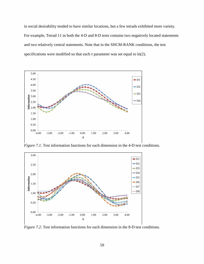
59
in social desirability tended to have similar locations, but a few tetrads exhibited more variety.
For example, Tetrad 11 in both the 4-D and 8-D tests contains two negatively located statements
and two relatively central statements. Note that in the SHCM-RANK conditions, the test
specifications were modified so that each τ parameter was set equal to ln(2).
Figure 7.1. Test information functions for each dimension in the 4-D test conditions.
Figure 7.2. Test information functions for each dimension in the 8-D test conditions.
0.00
0.50
1.00
1.50
2.00
2.50
3.00
3.50
4.00
4.50
5.00
-4.00 -3.00 -2.00 -1.00 0.00 1.00 2.00 3.00 4.00
Info
rmat
ion
θ
D1
D2
D3
D4
0.00
0.50
1.00
1.50
2.00
2.50
3.00
-4.00 -3.00 -2.00 -1.00 0.00 1.00 2.00 3.00 4.00
Info
rmat
ion
θ
D1D2D3D4D5D6D7D8
60
Simulation Details
Generating Rank Responses for MFC Tetrads
HCM-RANK and SHCM-RANK response data were generated as follows:
1. For the designated number of respondents and dimensions measured in each experimental
condition, trait scores were sampled randomly from independent standard normal
distributions. These trait scores are referred to henceforth as the “generating,” “known,”
or “true” trait scores.
2. For each MFC tetrad, the true trait scores and the true statement parameters were used to
compute HCM-PICK (Equation 5.1) or SHCM-PICK (Equation 5.2) probabilities. These
probabilities were used to divide a 0 to 1 probability interval into four segments, each
corresponding to a statement. A random uniform number was generated, the segment into
which the number fell was identified, and the corresponding statement was designated as
most like. That statement was designated as the highest ranked.
3. The PICK probabilities for the three remaining alternatives in the tetrad were
recomputed. A 0 to 1 probability interval was divided into three segments using those
values. A new random uniform number was generated, the segment into which the
number fell was identified, and the corresponding statement was designated as most like.
That statement was designated as the second-highest ranked.
4. The PICK probabilities for the two remaining alternatives in the tetrad were recomputed.
A 0 to 1 probability interval was divided into two segments using those values. A new
random uniform number was generated, the segment into which the number fell was
identified, and the corresponding statement was designated as most like. That statement
was designated as the third-highest ranked.

61
5. The remaining statement in the tetrad was designated as lowest ranked.
Generating Single-Statement Responses for Statement Precalibration in Two-Stage
Conditions
1. For the designated number of respondents and dimensions measured in each experimental
condition, trait scores were sampled randomly from independent standard normal
distributions. These trait scores are referred to henceforth as the “generating,” “known,”
or “true” trait scores.
2. For the statements measuring each dimension, the true trait scores and the true statement
parameters were used to compute HCM (Equation 4.5) or SHCM agreement (Equation
4.7) probabilities. These probabilities were compared to randomly generated uniform
numbers. In each case, if the probability exceeded the random number, then the response
was coded as 1 (agree); otherwise the response was coded as 0 (disagree).
Simulation Process in Direct Conditions
In Direct conditions, item and person parameters were estimated directly from the
generated rank responses. Data generation and parameter estimation proceeded as follows:
1. HCM-RANK and SHCM-RANK responses were generated for samples of 250 and 500
respondents using the 4-D and 8-D MFC tetrad tests described above.
2. Item and person parameters were estimated directly from the rank responses, using the
MCMC algorithms developed for this dissertation, and the results were saved.
3. Steps 1 and 2 were repeated until 30 replications were performed. Then indices of
estimation accuracy were computed.
62
Simulation Process in Two-Stage Conditions
In Two-Stage conditions, person parameters were estimated from tetrad rank responses
using precalibrated statement parameters. Data generation and parameter estimation proceeded
as follows:
1. Precalibration: Single-statement dichotomous responses were generated, one dimension
at a time, for samples of 250 and 500 respondents using true parameters for the
statements included in the 4-D and 8-D MFC tetrad tests. These dichotomous responses
were then calibrated using the HCM or SHCM to obtain statement parameter estimates
used for scoring “future samples” of MFC tetrad rank responses.
2. MFC test administration and scoring: HCM-RANK or SHCM-RANK responses were
generated for new samples of 250 and 500 respondents, for the 4-D and 8-D MFC tetrad
tests, using the true statement parameters. The rank response data were then scored with
the HCM-RANK or SHCM-RANK MCMC algorithm using the statement parameter
estimates from the precalibration phase. To examine the upper-bound of trait recovery,
responses were also scored using the true statement parameters.
3. Steps 1 and 2 were repeated until 30 replications were performed. Indices of estimation
accuracy were then computed.
Indices of Estimation Accuracy
Estimation accuracy was evaluated using three indices. First, Pearson correlations were
computed between the estimated and true item and person parameters averaged over replications.
Correlations above .9 are generally considered good to excellent in parameter recovery studies.
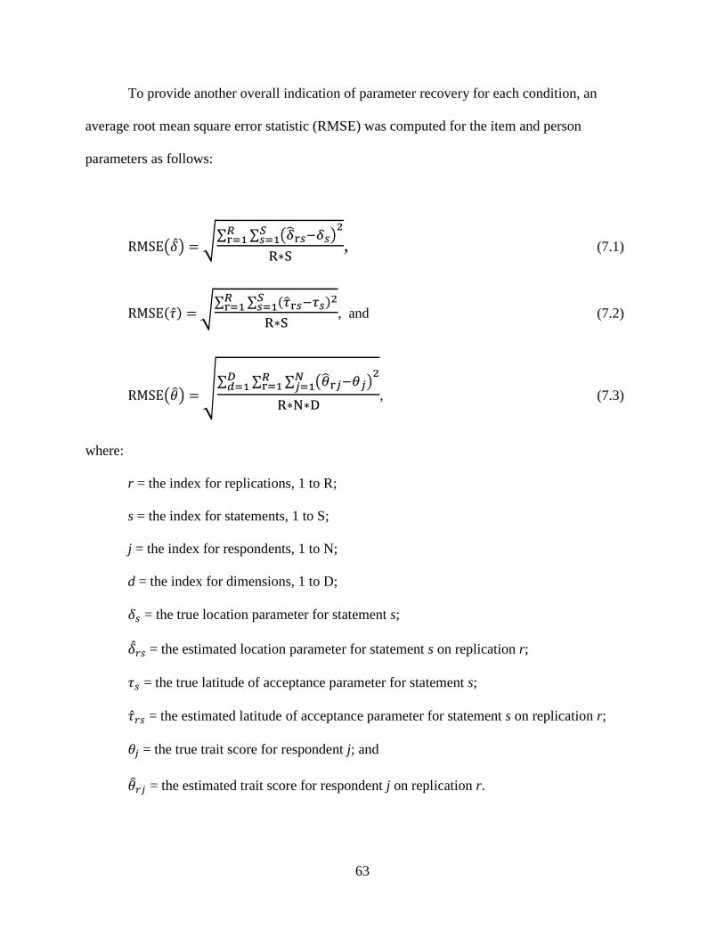
63
To provide another overall indication of parameter recovery for each condition, an
average root mean square error statistic (RMSE) was computed for the item and person
parameters as follows:
RMSE��̂�� = �∑ ∑ �𝛿�r𝑠−𝛿𝑠�2𝑆
𝑠=1𝑅r=1
R∗S, (7.1)
RMSE(�̂�) = �∑ ∑ (𝜏�r𝑠−𝜏𝑠)2𝑆𝑠=1
𝑅r=1
R∗S, and (7.2)
RMSE�𝜃�� = �∑ ∑ ∑ �𝜃�r𝑗−𝜃𝑗�
2𝑁𝑗=1
𝑅r=1
𝐷𝑑=1
R∗N∗D, (7.3)
where:
r = the index for replications, 1 to R;
s = the index for statements, 1 to S;
j = the index for respondents, 1 to N;
d = the index for dimensions, 1 to D;
𝛿𝑠 = the true location parameter for statement s;
𝛿𝑟𝑠 = the estimated location parameter for statement s on replication r;
𝜏𝑠 = the true latitude of acceptance parameter for statement s;
�̂�𝑟𝑠 = the estimated latitude of acceptance parameter for statement s on replication r;
𝜃𝑗 = the true trait score for respondent j; and
𝜃�𝑟𝑗 = the estimated trait score for respondent j on replication r.
64
Finally, to provide information about parameter recovery for individual statements which might
be helpful when choosing priors for MCMC estimation, the average statement parameter
estimate across replications was computed and a scatter-plot of the generating and average
estimates was examined.
MCMC Estimation Prior Distributions and Initial Parameter Values
For MCMC statement precalibration with the HCM in two-stage conditions, prior
distributions and starting values were chosen in accordance with Seybert et al. (manuscript in
preparation). Specifically, a bisection method, adapted from Roberts and Laughlin (1996), was
used to obtain starting values for statement location (δ) and latitude of acceptance (τ) parameters.
Starting values for person parameters (θ) were set at 0. For location parameters, normal priors
with means equal to the starting values and variances equal to 1 were chosen. For latitude of
acceptance parameters, four-parameter beta priors with support (-2, 5) and shape parameters (4,
3.5) were used. The prior distribution for person parameters was standard normal.
In direct estimation conditions with the HCM-RANK model, starting values and prior
distributions were based on research with the HCM and several pilot simulations. Independent
standard normal priors were chosen for person parameters (θ). Location parameters (δ) utilized a
weak four-parameter beta prior with support parameters (-5, 5) and shape parameters (2, 2). And
latitude of acceptance parameters (τ) utilized a four-parameter beta prior with support (-1, 5) and
shape parameters (4, 3.5). All person parameters were assigned starting values (θ 0) of 0. All
latitude of acceptance parameters were assigned starting values (τ0) of 2. Location parameters
were assigned starting values (δ0) of -3, 0, or +3, under the assumption that SMEs are able to
provide rough estimates of statement extremity. For simulation purposes, if the true location
parameter was below -1.00, a starting value of -3 was assigned. If the true location parameter
65
was between -1.00 and +1.00, a value of 0 was assigned. And if the true location parameter was
greater than 1.00, a starting value of 3 was assigned.
MCMC Estimation Burn-In and Chain Length
Two important considerations in MCMC estimation are the number of iterations needed
for chains to converge and the number of iterations following convergence from which
inferences about model parameters can be drawn. The sum of these numbers determines the
maximum number of iterations to run when estimating model parameters.
Convergence means that a chain has reached a stationary state so that samples are being
drawn from the desired posterior distributions. Since current states no longer depend on initial
states after convergence, the original choices of starting values and priors become irrelevant. The
iterations preceding convergence are commonly referred to as “burn-in” samples and are
typically discarded. “Post-burn-in” samples are used to compute means and standard deviations
of the posterior draws that represent the desired parameter estimates and standard errors,
respectively.
Several methods have been proposed for checking convergence and determining the
necessary numbers of burn-in and post-burn-in iterations. Simultaneously running multiple
chains starting with different initial states and examining the agreement after a designated
number of iterations has proven to be practical and effective (Patz & Junker, 1999a). In a review
of MCMC estimation for IRT models, Wollack, Bolt, Cohen, and Lee (2002) found that the
majority of studies utilized burn-in samples of 300 to 5,000 iterations. The number of post burn-
in samples frequently ranges from one-tenth to three-times as many iterations as used for burn-
in.
66
In preparation for this study, pilot simulations were conducted using three simultaneous
chains. For HCM-RANK direct estimation, it was found that convergence occurred at
approximately 20,000 iterations. For two-stage estimation, 20,000 iterations were also needed for
convergence during HCM statement precalibration, but only 2,000 were needed for subsequent
HCM-RANK scoring.
In this study, to insure that convergence occurred on every replication in every condition,
substantially more than the necessary numbers of burn-in and post-burn-in iterations were
performed. However, only one chain was run due to extremely long runtimes. In direct
estimation conditions, 100,000 total iterations were performed, and the first 50,000 were
discarded. The same specifications were used for HCM statement precalibration in the two-stage
estimation conditions. For HCM-RANK scoring in the two-stage conditions, 20,000 total
iterations were performed and 5,000 were discarded as burn-in.
Hypotheses
Due to a lack of studies examining the recovery of item and person parameters directly
from rank-order response data, experience with single-statement estimation was used to
formulate the following hypotheses.
1. Parameters will be estimated more accurately in the large sample (N=500) conditions
than in the small sample (N=250) conditions, as indicated by significantly larger Pearson
correlations between estimated and true parameters and significantly lower RMSE
statistics.
2. Parameters will be estimated more accurately (indicated by significantly larger Pearson
correlations between estimated and true parameters and significantly lower RMSE

67
statistics) with 4-D tests than with 8-D tests, because keeping test length constant (20
items) means that each dimension in the 8-D test is represented by fewer statements.
3. No significant differences will be found for person parameter recovery from rank
responses in the direct and two-stage estimation conditions.
4. No significant differences will be found for person parameter recovery in the HCM and
SHCM conditions.
5. Significant differences will be found for statement recovery in the direct and two-stage
estimation conditions.
6. In HCM conditions, statement location parameters will be estimated more accurately than
latitude of acceptance parameters, as indicated by significantly larger Pearson
correlations between estimated and true parameters and significantly lower RMSE
statistics.
Hypotheses were tested using MANOVA and the visual inspection of plots of statement bias.
Eta squared effect sizes were obtained to evaluate the overall influences of the independent
variables on study results.
68
CHAPTER 8:
STUDY 1 RESULTS
The purpose of this study was to examine the accuracy of HCM-RANK and SHCM-
RANK statement and person parameter recovery through a Monte Carlo simulation. The
recovery of parameters was examined by constructing MFC item tetrads according to the design
specifications detailed in Chapter 7. Following that, a direct estimation or two-stage estimation
process was used to generate and estimate response data and results were averaged over
replications and then compared to the generating values to obtain indices of estimation accuracy.
Simulation Results
Table 8.1 shows the overall statement parameter recovery statistics for each condition,
averaged across replications and the individual statements. The top portion of the table shows the
average correlations between the generating and estimated parameters, and the bottom portion
shows the root mean square error (RMSE) statistics. (Note that only HCM-RANK results are
shown for τ because the values were fixed at ln(2) for the SHCM-RANK estimation.) Overall, it
appears that statement location parameters (δ) were relatively well estimated, with correlations
above .95 in all cases and RMSEs as low as .161. Latitude of acceptance parameters, however,
were not as well estimated, with correlations ranging from .505 to .831, and RMSEs only as low
as .454. Location parameter estimates also had markedly smaller RMSEs in the SHCM-RANK
conditions than in the HCM-RANK conditions. As was expected, parameter estimates were
generally better with samples of 500 than 250, and with 4-D tests than 8-D tests. Finally, for the
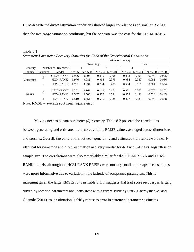
69
HCM-RANK the direct estimation conditions showed larger correlations and smaller RMSEs
than the two-stage estimation conditions, but the opposite was the case for the SHCM-RANK.
Table 8.1 Statement Parameter Recovery Statistics for Each of the Experimental Conditions
Note. RMSE = average root mean square error.
Moving next to person parameter (θ) recovery, Table 8.2 presents the correlations
between generating and estimated trait scores and the RMSE values, averaged across dimensions
and persons. Overall, the correlations between generating and estimated trait scores were nearly
identical for two-stage and direct estimation and very similar for 4-D and 8-D tests, regardless of
sample size. The correlations were also remarkably similar for the SHCM-RANK and HCM-
RANK models, although the HCM-RANK RMSEs were notably smaller, perhaps because items
were more informative due to variation in the latitude of acceptance parameters. This is
intriguing given the large RMSEs for τ in Table 8.1. It suggests that trait score recovery is largely
driven by location parameters and, consistent with a recent study by Stark, Chernyshenko, and
Guenole (2011), trait estimation is fairly robust to error in statement parameter estimates.
Parameter Model N = 250 N = 500 N = 250 N = 500 N = 250 N = 500 N = 250 N = 500SHCM-RANK 0.996 0.998 0.995 0.998 0.993 0.995 0.990 0.995HCM-RANK 0.976 0.982 0.968 0.975 0.984 0.987 0.981 0.986
τ HCM-RANK 0.781 0.831 0.734 0.785 0.504 0.511 0.504 0.554
SHCM-RANK 0.231 0.161 0.249 0.171 0.321 0.262 0.370 0.282HCM-RANK 0.587 0.500 0.677 0.594 0.478 0.433 0.528 0.443
τ HCM-RANK 0.510 0.454 0.595 0.538 0.927 0.935 0.898 0.878
Estimation Strategy
δ
δ
Correlation
RMSE
Number of Dimensions:Two-Stage Direct
4 8 4 8Recovery Statistic
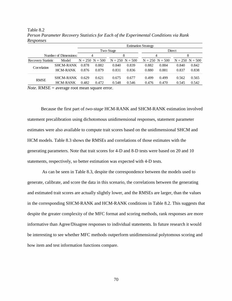
70
Table 8.2 Person Parameter Recovery Statistics for Each of the Experimental Conditions via Rank Responses
Note. RMSE = average root mean square error.
Because the first part of two-stage HCM-RANK and SHCM-RANK estimation involved
statement precalibration using dichotomous unidimensional responses, statement parameter
estimates were also available to compute trait scores based on the unidimensional SHCM and
HCM models. Table 8.3 shows the RMSEs and correlations of those estimates with the
generating parameters. Note that trait scores for 4-D and 8-D tests were based on 20 and 10
statements, respectively, so better estimation was expected with 4-D tests.
As can be seen in Table 8.3, despite the correspondence between the models used to
generate, calibrate, and score the data in this scenario, the correlations between the generating
and estimated trait scores are actually slightly lower, and the RMSEs are larger, than the values
in the corresponding SHCM-RANK and HCM-RANK conditions in Table 8.2. This suggests that
despite the greater complexity of the MFC format and scoring methods, rank responses are more
informative than Agree/Disagree responses to individual statements. In future research it would
be interesting to see whether MFC methods outperform unidimensional polytomous scoring and
how item and test information functions compare.
Recovery Statistic Model N = 250 N = 500 N = 250 N = 500 N = 250 N = 500 N = 250 N = 500SHCM-RANK 0.878 0.882 0.840 0.839 0.882 0.884 0.840 0.842HCM-RANK 0.876 0.879 0.831 0.836 0.880 0.881 0.837 0.838
SHCM-RANK 0.629 0.621 0.675 0.677 0.499 0.499 0.562 0.565HCM-RANK 0.482 0.472 0.548 0.546 0.476 0.470 0.545 0.542
Correlation
RMSE
Number of Dimensions:
Estimation StrategyTwo-Stage Direct
4 8 4 8
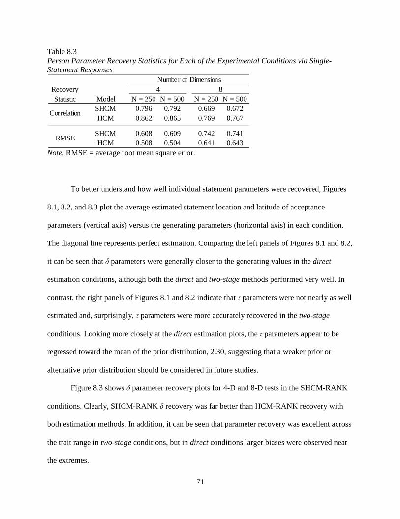
71
Table 8.3 Person Parameter Recovery Statistics for Each of the Experimental Conditions via Single-Statement Responses
Note. RMSE = average root mean square error.
To better understand how well individual statement parameters were recovered, Figures
8.1, 8.2, and 8.3 plot the average estimated statement location and latitude of acceptance
parameters (vertical axis) versus the generating parameters (horizontal axis) in each condition.
The diagonal line represents perfect estimation. Comparing the left panels of Figures 8.1 and 8.2,
it can be seen that δ parameters were generally closer to the generating values in the direct
estimation conditions, although both the direct and two-stage methods performed very well. In
contrast, the right panels of Figures 8.1 and 8.2 indicate that τ parameters were not nearly as well
estimated and, surprisingly, τ parameters were more accurately recovered in the two-stage
conditions. Looking more closely at the direct estimation plots, the τ parameters appear to be
regressed toward the mean of the prior distribution, 2.30, suggesting that a weaker prior or
alternative prior distribution should be considered in future studies.
Figure 8.3 shows δ parameter recovery plots for 4-D and 8-D tests in the SHCM-RANK
conditions. Clearly, SHCM-RANK δ recovery was far better than HCM-RANK recovery with
both estimation methods. In addition, it can be seen that parameter recovery was excellent across
the trait range in two-stage conditions, but in direct conditions larger biases were observed near
the extremes.
Model N = 250 N = 500 N = 250 N = 500SHCM 0.796 0.792 0.669 0.672HCM 0.862 0.865 0.769 0.767
SHCM 0.608 0.609 0.742 0.741HCM 0.508 0.504 0.641 0.643
Correlation
RMSE
Number of Dimensions4 8Recovery
Statistic
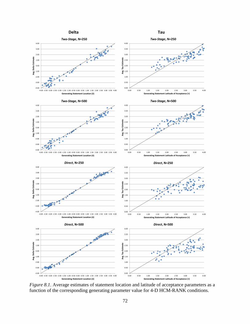
72
Figure 8.1. Average estimates of statement location and latitude of acceptance parameters as a function of the corresponding generating parameter value for 4-D HCM-RANK conditions.
-4.00
-3.00
-2.00
-1.00
0.00
1.00
2.00
3.00
4.00
-4.00 -3.50 -3.00 -2.50 -2.00 -1.50 -1.00 -0.50 0.00 0.50 1.00 1.50 2.00 2.50 3.00 3.50 4.00
Avg.
Del
ta E
stim
ate
Generating Statement Location (δ)
Two-Stage, N=250
Delta Tau
-4.00
-3.00
-2.00
-1.00
0.00
1.00
2.00
3.00
4.00
-4.00 -3.50 -3.00 -2.50 -2.00 -1.50 -1.00 -0.50 0.00 0.50 1.00 1.50 2.00 2.50 3.00 3.50 4.00
Avg.
Del
ta E
stim
ate
Generating Statement Location (δ)
Two-Stage, N=500
-4.00
-3.00
-2.00
-1.00
0.00
1.00
2.00
3.00
4.00
-4.00 -3.50 -3.00 -2.50 -2.00 -1.50 -1.00 -0.50 0.00 0.50 1.00 1.50 2.00 2.50 3.00 3.50 4.00
Avg.
Del
ta E
stim
ate
Generating Statement Location (δ)
Direct, N=250
-4.00
-3.00
-2.00
-1.00
0.00
1.00
2.00
3.00
4.00
-4.00 -3.50 -3.00 -2.50 -2.00 -1.50 -1.00 -0.50 0.00 0.50 1.00 1.50 2.00 2.50 3.00 3.50 4.00
Avg.
Del
ta E
stim
ate
Generating Statement Location (δ)
Direct, N=500
0.00
0.50
1.00
1.50
2.00
2.50
3.00
3.50
4.00
0.00 0.50 1.00 1.50 2.00 2.50 3.00 3.50 4.00
Avg.
Tau
Est
imat
e
Generating Statement Latitude of Acceptance (τ)
Two-Stage, N=250
0.00
0.50
1.00
1.50
2.00
2.50
3.00
3.50
4.00
0.00 0.50 1.00 1.50 2.00 2.50 3.00 3.50 4.00
Avg.
Tau
Est
imat
e
Generating Statement Latitude of Acceptance (τ)
Two-Stage, N=500
0.00
0.50
1.00
1.50
2.00
2.50
3.00
3.50
4.00
0.00 0.50 1.00 1.50 2.00 2.50 3.00 3.50 4.00
Avg.
Tau
Est
imat
e
Generating Statement Latitude of Acceptance (τ)
Direct, N=250
0.00
0.50
1.00
1.50
2.00
2.50
3.00
3.50
4.00
0.00 0.50 1.00 1.50 2.00 2.50 3.00 3.50 4.00
Avg.
Tau
Est
imat
e
Generating Statement Latitude of Acceptance (τ)
Direct, N=500
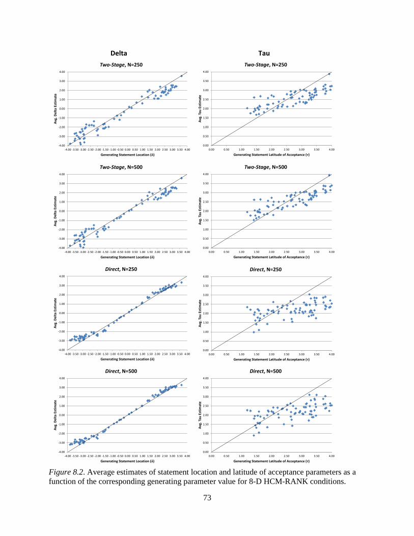
73
Figure 8.2. Average estimates of statement location and latitude of acceptance parameters as a function of the corresponding generating parameter value for 8-D HCM-RANK conditions.
-4.00
-3.00
-2.00
-1.00
0.00
1.00
2.00
3.00
4.00
-4.00 -3.50 -3.00 -2.50 -2.00 -1.50 -1.00 -0.50 0.00 0.50 1.00 1.50 2.00 2.50 3.00 3.50 4.00
Avg.
Del
ta E
stim
ate
Generating Statement Location (δ)
Two-Stage, N=250
Delta Tau
-4.00
-3.00
-2.00
-1.00
0.00
1.00
2.00
3.00
4.00
-4.00 -3.50 -3.00 -2.50 -2.00 -1.50 -1.00 -0.50 0.00 0.50 1.00 1.50 2.00 2.50 3.00 3.50 4.00
Avg.
Del
ta E
stim
ate
Generating Statement Location (δ)
Two-Stage, N=500
-4.00
-3.00
-2.00
-1.00
0.00
1.00
2.00
3.00
4.00
-4.00 -3.50 -3.00 -2.50 -2.00 -1.50 -1.00 -0.50 0.00 0.50 1.00 1.50 2.00 2.50 3.00 3.50 4.00
Avg.
Del
ta E
stim
ate
Generating Statement Location (δ)
Direct, N=250
-4.00
-3.00
-2.00
-1.00
0.00
1.00
2.00
3.00
4.00
-4.00 -3.50 -3.00 -2.50 -2.00 -1.50 -1.00 -0.50 0.00 0.50 1.00 1.50 2.00 2.50 3.00 3.50 4.00
Avg.
Del
ta E
stim
ate
Generating Statement Location (δ)
Direct, N=500
0.00
0.50
1.00
1.50
2.00
2.50
3.00
3.50
4.00
0.00 0.50 1.00 1.50 2.00 2.50 3.00 3.50 4.00
Avg.
Tau
Est
imat
e
Generating Statement Latitude of Acceptance (τ)
Two-Stage, N=250
0.00
0.50
1.00
1.50
2.00
2.50
3.00
3.50
4.00
0.00 0.50 1.00 1.50 2.00 2.50 3.00 3.50 4.00
Avg.
Tau
Est
imat
e
Generating Statement Latitude of Acceptance (τ)
Two-Stage, N=500
0.00
0.50
1.00
1.50
2.00
2.50
3.00
3.50
4.00
0.00 0.50 1.00 1.50 2.00 2.50 3.00 3.50 4.00
Avg.
Tau
Est
imat
e
Generating Statement Latitude of Acceptance (τ)
Direct, N=250
0.00
0.50
1.00
1.50
2.00
2.50
3.00
3.50
4.00
0.00 0.50 1.00 1.50 2.00 2.50 3.00 3.50 4.00
Avg.
Tau
Est
imat
e
Generating Statement Latitude of Acceptance (τ)
Direct, N=500
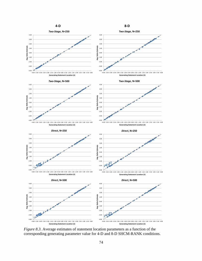
74
Figure 8.3. Average estimates of statement location parameters as a function of the corresponding generating parameter value for 4-D and 8-D SHCM-RANK conditions.
-4.00
-3.00
-2.00
-1.00
0.00
1.00
2.00
3.00
4.00
-4.00 -3.50 -3.00 -2.50 -2.00 -1.50 -1.00 -0.50 0.00 0.50 1.00 1.50 2.00 2.50 3.00 3.50 4.00
Avg.
Del
ta E
stim
ate
Generating Statement Location (δ)
Two-Stage, N=250
4-D 8-D
-4.00
-3.00
-2.00
-1.00
0.00
1.00
2.00
3.00
4.00
-4.00 -3.50 -3.00 -2.50 -2.00 -1.50 -1.00 -0.50 0.00 0.50 1.00 1.50 2.00 2.50 3.00 3.50 4.00
Avg.
Del
ta E
stim
ate
Generating Statement Location (δ)
Two-Stage, N=500
-4.00
-3.00
-2.00
-1.00
0.00
1.00
2.00
3.00
4.00
-4.00 -3.50 -3.00 -2.50 -2.00 -1.50 -1.00 -0.50 0.00 0.50 1.00 1.50 2.00 2.50 3.00 3.50 4.00
Avg.
Del
ta E
stim
ate
Generating Statement Location (δ)
Direct, N=250
-4.00
-3.00
-2.00
-1.00
0.00
1.00
2.00
3.00
4.00
-4.00 -3.50 -3.00 -2.50 -2.00 -1.50 -1.00 -0.50 0.00 0.50 1.00 1.50 2.00 2.50 3.00 3.50 4.00
Avg.
Del
ta E
stim
ate
Generating Statement Location (δ)
Direct, N=500
-4.00
-3.00
-2.00
-1.00
0.00
1.00
2.00
3.00
4.00
-4.00 -3.50 -3.00 -2.50 -2.00 -1.50 -1.00 -0.50 0.00 0.50 1.00 1.50 2.00 2.50 3.00 3.50 4.00
Avg.
Del
ta E
stim
ate
Generating Statement Location (δ)
Two-Stage, N=250
-4.00
-3.00
-2.00
-1.00
0.00
1.00
2.00
3.00
4.00
-4.00 -3.50 -3.00 -2.50 -2.00 -1.50 -1.00 -0.50 0.00 0.50 1.00 1.50 2.00 2.50 3.00 3.50 4.00
Avg.
Del
ta E
stim
ate
Generating Statement Location (δ)
Two-Stage, N=500
-4.00
-3.00
-2.00
-1.00
0.00
1.00
2.00
3.00
4.00
-4.00 -3.50 -3.00 -2.50 -2.00 -1.50 -1.00 -0.50 0.00 0.50 1.00 1.50 2.00 2.50 3.00 3.50 4.00
Avg.
Del
ta E
stim
ate
Generating Statement Location (δ)
Direct, N=250
-4.00
-3.00
-2.00
-1.00
0.00
1.00
2.00
3.00
4.00
-4.00 -3.50 -3.00 -2.50 -2.00 -1.50 -1.00 -0.50 0.00 0.50 1.00 1.50 2.00 2.50 3.00 3.50 4.00
Avg.
Del
ta E
stim
ate
Generating Statement Location (δ)
Direct, N=500
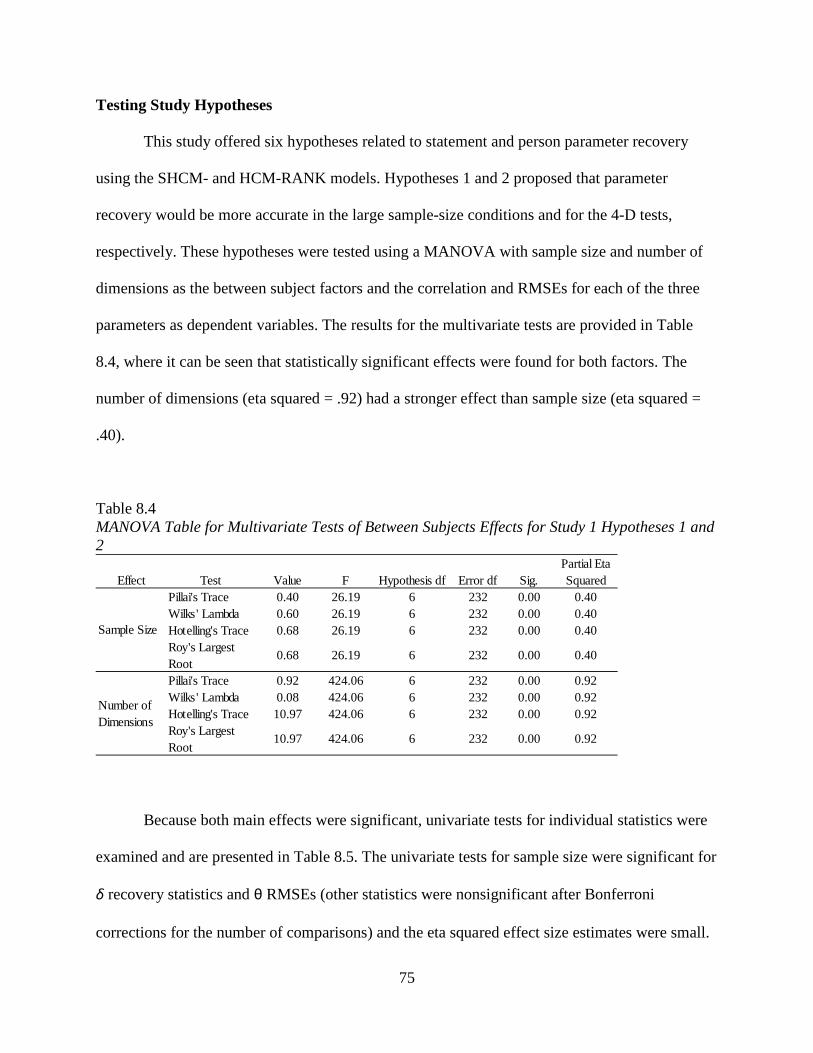
75
Testing Study Hypotheses
This study offered six hypotheses related to statement and person parameter recovery
using the SHCM- and HCM-RANK models. Hypotheses 1 and 2 proposed that parameter
recovery would be more accurate in the large sample-size conditions and for the 4-D tests,
respectively. These hypotheses were tested using a MANOVA with sample size and number of
dimensions as the between subject factors and the correlation and RMSEs for each of the three
parameters as dependent variables. The results for the multivariate tests are provided in Table
8.4, where it can be seen that statistically significant effects were found for both factors. The
number of dimensions (eta squared = .92) had a stronger effect than sample size (eta squared =
.40).
Table 8.4 MANOVA Table for Multivariate Tests of Between Subjects Effects for Study 1 Hypotheses 1 and 2
Because both main effects were significant, univariate tests for individual statistics were
examined and are presented in Table 8.5. The univariate tests for sample size were significant for
δ recovery statistics and θ RMSEs (other statistics were nonsignificant after Bonferroni
corrections for the number of comparisons) and the eta squared effect size estimates were small.
Effect Test Value F Hypothesis df Error df Sig.Partial Eta Squared
Pillai's Trace 0.40 26.19 6 232 0.00 0.40Wilks' Lambda 0.60 26.19 6 232 0.00 0.40Hotelling's Trace 0.68 26.19 6 232 0.00 0.40Roy's Largest Root
0.68 26.19 6 232 0.00 0.40
Pillai's Trace 0.92 424.06 6 232 0.00 0.92Wilks' Lambda 0.08 424.06 6 232 0.00 0.92Hotelling's Trace 10.97 424.06 6 232 0.00 0.92Roy's Largest Root
10.97 424.06 6 232 0.00 0.92
Sample Size
Number of Dimensions
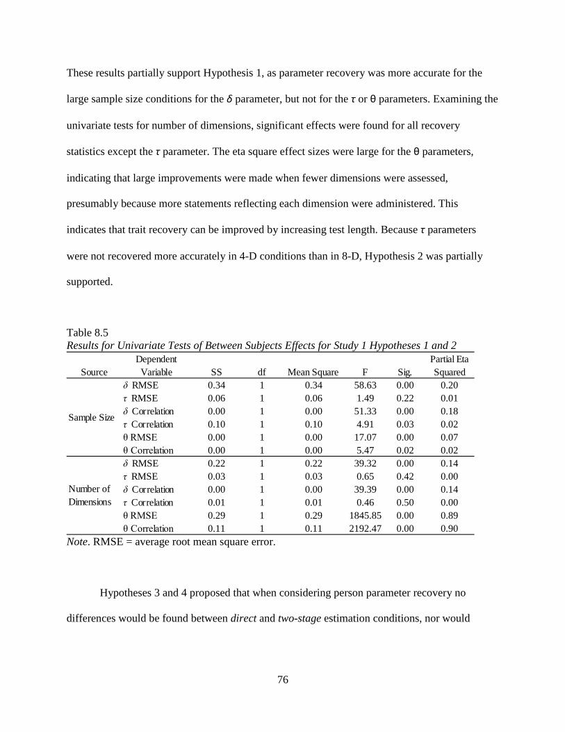
76
These results partially support Hypothesis 1, as parameter recovery was more accurate for the
large sample size conditions for the δ parameter, but not for the τ or θ parameters. Examining the
univariate tests for number of dimensions, significant effects were found for all recovery
statistics except the τ parameter. The eta square effect sizes were large for the θ parameters,
indicating that large improvements were made when fewer dimensions were assessed,
presumably because more statements reflecting each dimension were administered. This
indicates that trait recovery can be improved by increasing test length. Because τ parameters
were not recovered more accurately in 4-D conditions than in 8-D, Hypothesis 2 was partially
supported.
Table 8.5 Results for Univariate Tests of Between Subjects Effects for Study 1 Hypotheses 1 and 2
Note. RMSE = average root mean square error.
Hypotheses 3 and 4 proposed that when considering person parameter recovery no
differences would be found between direct and two-stage estimation conditions, nor would
SourceDependent Variable SS df Mean Square F Sig.
Partial Eta Squared
δ RMSE 0.34 1 0.34 58.63 0.00 0.20τ RMSE 0.06 1 0.06 1.49 0.22 0.01δ Correlation 0.00 1 0.00 51.33 0.00 0.18τ Correlation 0.10 1 0.10 4.91 0.03 0.02θ RMSE 0.00 1 0.00 17.07 0.00 0.07θ Correlation 0.00 1 0.00 5.47 0.02 0.02δ RMSE 0.22 1 0.22 39.32 0.00 0.14τ RMSE 0.03 1 0.03 0.65 0.42 0.00δ Correlation 0.00 1 0.00 39.39 0.00 0.14τ Correlation 0.01 1 0.01 0.46 0.50 0.00θ RMSE 0.29 1 0.29 1845.85 0.00 0.89θ Correlation 0.11 1 0.11 2192.47 0.00 0.90
Number of Dimensions
Sample Size
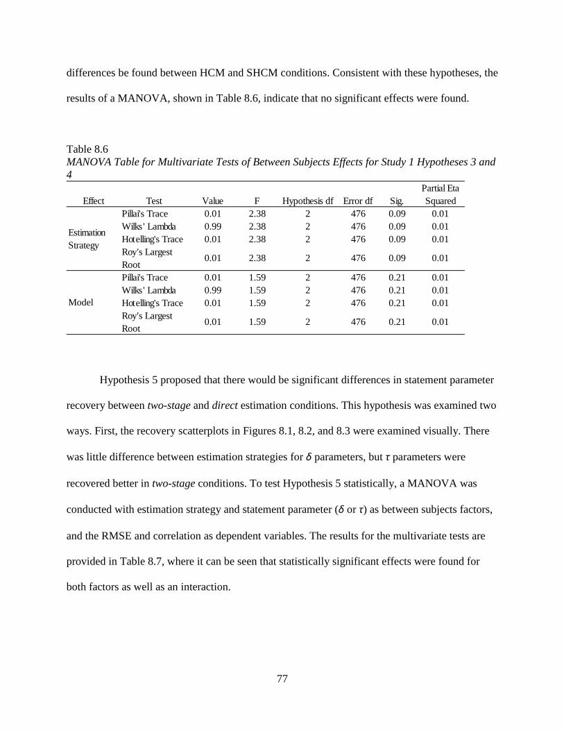
77
differences be found between HCM and SHCM conditions. Consistent with these hypotheses, the
results of a MANOVA, shown in Table 8.6, indicate that no significant effects were found.
Table 8.6 MANOVA Table for Multivariate Tests of Between Subjects Effects for Study 1 Hypotheses 3 and 4
Hypothesis 5 proposed that there would be significant differences in statement parameter
recovery between two-stage and direct estimation conditions. This hypothesis was examined two
ways. First, the recovery scatterplots in Figures 8.1, 8.2, and 8.3 were examined visually. There
was little difference between estimation strategies for δ parameters, but τ parameters were
recovered better in two-stage conditions. To test Hypothesis 5 statistically, a MANOVA was
conducted with estimation strategy and statement parameter (δ or τ) as between subjects factors,
and the RMSE and correlation as dependent variables. The results for the multivariate tests are
provided in Table 8.7, where it can be seen that statistically significant effects were found for
both factors as well as an interaction.
Effect Test Value F Hypothesis df Error df Sig.Partial Eta Squared
Pillai's Trace 0.01 2.38 2 476 0.09 0.01Wilks' Lambda 0.99 2.38 2 476 0.09 0.01Hotelling's Trace 0.01 2.38 2 476 0.09 0.01Roy's Largest Root
0.01 2.38 2 476 0.09 0.01
Pillai's Trace 0.01 1.59 2 476 0.21 0.01Wilks' Lambda 0.99 1.59 2 476 0.21 0.01Hotelling's Trace 0.01 1.59 2 476 0.21 0.01Roy's Largest Root
0.01 1.59 2 476 0.21 0.01
Estimation Strategy
Model
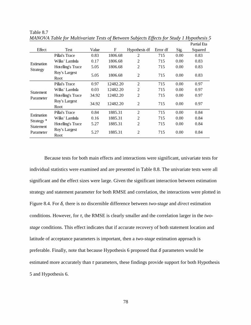
78
Table 8.7 MANOVA Table for Multivariate Tests of Between Subjects Effects for Study 1 Hypothesis 5
Because tests for both main effects and interactions were significant, univariate tests for
individual statistics were examined and are presented in Table 8.8. The univariate tests were all
significant and the effect sizes were large. Given the significant interaction between estimation
strategy and statement parameter for both RMSE and correlation, the interactions were plotted in
Figure 8.4. For δ, there is no discernible difference between two-stage and direct estimation
conditions. However, for τ, the RMSE is clearly smaller and the correlation larger in the two-
stage conditions. This effect indicates that if accurate recovery of both statement location and
latitude of acceptance parameters is important, then a two-stage estimation approach is
preferable. Finally, note that because Hypothesis 6 proposed that δ parameters would be
estimated more accurately than τ parameters, these findings provide support for both Hypothesis
5 and Hypothesis 6.
Effect Test Value F Hypothesis df Error df Sig.Partial Eta Squared
Pillai's Trace 0.83 1806.68 2 715 0.00 0.83Wilks' Lambda 0.17 1806.68 2 715 0.00 0.83Hotelling's Trace 5.05 1806.68 2 715 0.00 0.83Roy's Largest Root
5.05 1806.68 2 715 0.00 0.83
Pillai's Trace 0.97 12482.20 2 715 0.00 0.97Wilks' Lambda 0.03 12482.20 2 715 0.00 0.97Hotelling's Trace 34.92 12482.20 2 715 0.00 0.97Roy's Largest Root
34.92 12482.20 2 715 0.00 0.97
Pillai's Trace 0.84 1885.31 2 715 0.00 0.84Wilks' Lambda 0.16 1885.31 2 715 0.00 0.84Hotelling's Trace 5.27 1885.31 2 715 0.00 0.84Roy's Largest Root
5.27 1885.31 2 715 0.00 0.84
Estimation Strategy * Statement Parameter
Estimation Strategy
Statement Parameter
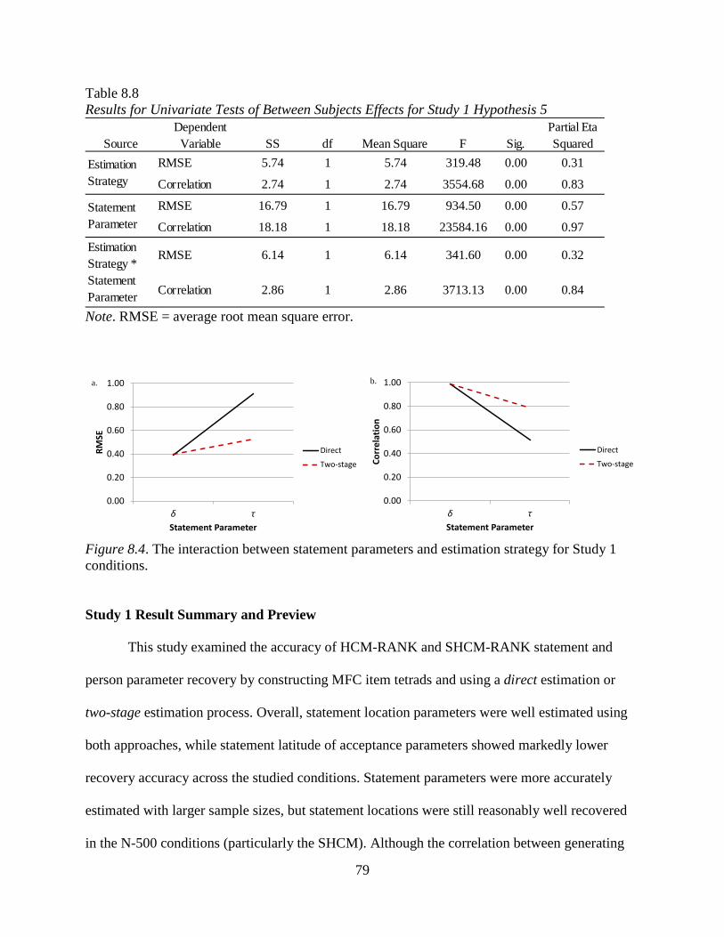
79
Table 8.8 Results for Univariate Tests of Between Subjects Effects for Study 1 Hypothesis 5
Note. RMSE = average root mean square error.
Figure 8.4. The interaction between statement parameters and estimation strategy for Study 1 conditions.
Study 1 Result Summary and Preview
This study examined the accuracy of HCM-RANK and SHCM-RANK statement and
person parameter recovery by constructing MFC item tetrads and using a direct estimation or
two-stage estimation process. Overall, statement location parameters were well estimated using
both approaches, while statement latitude of acceptance parameters showed markedly lower
recovery accuracy across the studied conditions. Statement parameters were more accurately
estimated with larger sample sizes, but statement locations were still reasonably well recovered
in the N-500 conditions (particularly the SHCM). Although the correlation between generating
SourceDependent
Variable SS df Mean Square F Sig.Partial Eta Squared
RMSE 5.74 1 5.74 319.48 0.00 0.31
Correlation 2.74 1 2.74 3554.68 0.00 0.83
RMSE 16.79 1 16.79 934.50 0.00 0.57
Correlation 18.18 1 18.18 23584.16 0.00 0.97
RMSE 6.14 1 6.14 341.60 0.00 0.32
Correlation 2.86 1 2.86 3713.13 0.00 0.84
Estimation Strategy
Statement Parameter
Estimation Strategy * Statement Parameter
0.00
0.20
0.40
0.60
0.80
1.00
δ τ
RMSE
Statement Parameter
Direct
Two-stage
0.00
0.20
0.40
0.60
0.80
1.00
δ τ
Corr
elat
ion
Statement Parameter
Direct
Two-stage
a. b.
80
and estimated person parameters never reached .90, correlations in the mid to high .80s indicate
fairly good recovery considering test length. By increasing test length it is expected that both
statement and person parameter recovery accuracy would also increase.
These results demonstrate the efficacy of the HCM-RANK and SHCM-RANK MCMC
estimation methods for MFC item tetrads and are consistent with previous studies focusing
specifically on trait score recovery. Stark, Chernyshenko, and Drasgow (2005) reported
correlations between generating and estimated trait scores ranging from .77 to .86 for a 2-D
pairwise preference test with 20 statements representing each dimension. Additionally, Stark,
Chernyshenko, Drasgow, and White (2012) found correlations of .68 to .92 for simulations of 2-
D to 25-D pairwise preference tests with uncorrelated latent dimensions. Using the Thurstonian
approach, Brown and Maydeu-Olivares (2011) found correlations ranging from .80 to .95 across
simulations of 5-D tests using item pairs, triplets, and tetrads. Most comparable to the current
study, de la Torre et al. (2012) found average correlations of .86 and .87 for 4-D pairwise
preference and tetrad-ranking conditions, respectively, when utilizing the GGUM as the
foundation for data generation and scoring. Results from the current study show comparable
correlations between generating and estimated latent trait scores, ranging from .83 to .88 across
the two-stage and direct estimation approaches.
One finding of particular interest in this study is that there were no significant differences
between estimation strategies in regard to person parameter recovery, indicating that MFC scales
can be constructed and administered without the need to for statement precalibration. A
sufficient number of MFC responses, however, must first be gathered before statement parameter
estimation and person scoring can occur. In Chapter 9, one potential strategy for obtaining initial

81
score estimates prior to the estimation of statement parameters is described, and a simulation
study is performed to examine the efficacy of the approach.
82
CHAPTER 9:
STUDY 2: EXAMINING SHCM-RANK TRAIT SCORE RECOVERY
USING SME LOCATION ESTIMATES
Item response theory methods offer many benefits for test development, but a key
drawback is that large samples are needed to accurately estimate the item parameters that are
used for scoring. With 250 examinees considered a fairly small sample in the IRT realm, the cost
of developing one item can easily exceed $100, thus forcing organizations to accept longer lags
for return on investment or, in the case of admissions and licensure testing, forcing examinees to
pay higher prices.
In Study 1, two approaches to item parameter estimation were examined in connection
with the scoring of MFC rank responses. In direct estimation conditions, an MFC tetrad test was
administered to a large sample of respondents and item and person parameters were estimated
simultaneously (directly) from the rank responses. In two-stage conditions, individual statements
were administered to a large sample of respondents and calibrated using a unidimensional single-
statement model; then the statement parameters from the precalibration were used to score MFC
rank responses. Consequently, despite procedural differences, both direct and two-stage
estimation used samples of 250 or more for estimating the item parameters that were needed for
scoring.
In recognition of this practical limitation and the desire for organizations to expedite test
development and launch, Stark, Chernyshenko, and Guenole (2011) explored the use of subject
matter expert (SME) location estimates in place of marginal maximum likelihood (MML)
83
location parameter estimates with the Zinnes and Griggs (ZG; 1974) unidimensional pairwise
preference model. They found that trait scores based on SME locations correlated .97 and .93
with trait scores based on MML locations, even though the correlations between the SME and
MML locations were just .83 and .62, respectively. Moreover, in a follow-up computer
simulation, the researchers found that trait score estimates based on SME locations, which
correlated only .6 with the true locations parameters, were comparable to trait scores calculated
using MML location estimates based on samples of 500 examinees. Together, these results
suggest that SME location estimates might serve as viable proxies for IRT location estimates in
the early stages of testing and possibly beyond. An important follow-up question is whether
these results will generalize to other models and more complex assessments.
Models that have been explored for MFC testing, to date, have all involved multiple
parameters. Stark (2002) and de la Torre et al. (2012) computed most like probabilities based on
the Generalized Graded Unfolding Model (GGUM; Roberts, Donoghue, & Laughlin, 2000),
which has three parameters for every statement (location, threshold, and discrimination).
Similarly, Brown and Maydeu-Olivares (2011) used a normal ogive model involving two
parameters per statement (an intercept and a factor loading). Consequently, research is needed to
explore whether simpler models, involving just location parameters, can provide effective
scoring of MFC responses, and to what extent estimation accuracy will diminish if SME location
estimates are substituted for IRT location parameters.
The SHCM-RANK model is a natural choice for this type of study. Like the ZG model,
explored by Stark et al. (2011) the SHCM has just one parameter per statement, representing its
location on the trait continuum. Thus, Study 2 of this dissertation explores whether MFC test

84
construction and scoring can be streamlined by substituting SME location estimates for MCMC-
based SHCM statement locations, as described below.
Simulation Study
Study Design
A Monte Carlo study was conducted to explore the efficacy of SHCM-RANK trait score
recovery with 4-D and 8-D MFC tests using SME-based SHCM location parameter estimates
having varying correlations with the true location parameters. The simulation involved two
independent variables with levels, as shown:
1) Dimensionality of MFC assessment:
a) 4 dimensions; and
b) 8 dimensions.
2) Location parameters used for SHCM-RANK scoring:
a) TRUE location parameters;
b) SME90: location estimates correlating .90 with true location parameters;
c) SME80: location estimates correlating .80 with true location parameters;
d) SME70: location estimates correlating .70 with true location parameters;
e) SME60: location estimates correlating .60 with true location parameters; and
f) SME50: location estimates correlating .50 with true location parameters.
Simulation Procedure
1) For each dimension in the MFC test, SME location parameter estimates having the
desired correlation with the true location parameters were created as follows: An
appropriately sized vector of values (z) was sampled from an independent standard
normal distribution and the following transformation was applied, 𝐬 = ρ𝐭 + �(1 − ρ2)𝐳 ,
85
where t represents the true location parameters, ρ represents the desired correlation, and s
represents the resulting vector of SME location estimates.
2) For the designated number of dimensions in the MFC test, trait scores for 1,000
examinees were sampled from independent standard normal distributions. SHCM-RANK
responses were generated using the true trait scores and true location parameters, as
described in Study 1.
3) The SHCM-RANK responses were scored using the TRUE or SME location estimates
and the results were saved.
4) Steps 1 through 3 were repeated until 30 replications were performed. Indices of
estimation accuracy were then computed.
Indices of Estimation Accuracy
As in Study 1, trait score recovery were examined using a combination of Pearson
correlations between average estimated and true trait scores and root mean square errors given by
Equation 7.3.
Hypotheses
Based on Stark et al. (2011), who used SME location estimates to score unidimensional
forced choice scales, the follow hypotheses are proposed:
1. Trait scores will be estimated more accurately with 4-D tests than with 8-D tests (as
indicated by significantly larger Pearson correlations between estimated and true trait
scores and significantly lower RMSE statistics), because keeping test length constant (20
items) means that each dimension in the 8-D test is represented by fewer statements.
2. Trait score estimation accuracy will decrease as the correlation between the SME
locations and TRUE locations decreases.

86
These hypotheses were tested using MANOVA and, for Hypothesis 2, orthogonal
polynomial contrasts to test the linear trend.
87
CHAPTER 10:
STUDY 2 RESULTS
The purpose of this study was to examine whether SME location estimates containing
varying degrees of error can be used effectively to score MFC responses with the SHCM-RANK
model. Correlations between estimated and generating trait scores were computed as were root
mean square errors (RMSE). Table 10.1 presents the parameter recovery results for the 12
simulation conditions, averaged across replications and dimensions. As expected, recovery was
best with the TRUE parameters and better with 4-D than 8-D tests in the corresponding SME
conditions. Importantly, parameter recovery diminished only minimally each time the correlation
between the true and SME location estimates was decreased by .1, indicating the robustness of
trait scores to measurement error. Remarkably correlations between the true and estimated trait
scores were at or above .8 even when SME locations correlated only .7 with the true values.
Testing Study Hypotheses
Two hypotheses were proposed for this study. Hypothesis 1 stated that person parameter
recovery would be more accurate with 4-D measures than 8-D measures. This hypothesis was
tested using a MANOVA with number of dimensions as the between subjects factor and the
correlation and RMSE statistics for person parameters as dependent variables. The multivariate
test results in Table 10.2 show that the effect for dimensions was significant, with a moderate
effect size (eta squared = .33). Consequently, univariate tests were conducted, and these results
are presented in Table 10.3. As can be seen in the table, significant effects were found for both
the correlation and RMSE, providing support for Hypothesis 1.
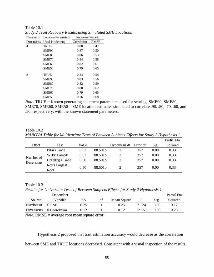
88
Table 10.1 Study 2 Trait Recovery Results using Simulated SME Locations
Note. TRUE = Known generating statement parameters used for scoring. SME90, SME80, SME70, SME60, SME50 = SME location estimates simulated to correlate .90, .80, .70, .60, and .50, respectively, with the known statement parameters.
Table 10.2 MANOVA Table for Multivariate Tests of Between Subjects Effects for Study 2 Hypothesis 1
Table 10.3 Results for Univariate Tests of Between Subjects Effects for Study 2 Hypothesis 1
Note. RMSE = average root mean square error.
Hypothesis 2 proposed that trait estimation accuracy would decrease as the correlation
between SME and TRUE locations decreased. Consistent with a visual inspection of the results,
Correlation RMSE4 TRUE 0.88 0.47
SME90 0.87 0.50SME80 0.86 0.53SME70 0.84 0.58SME60 0.82 0.61SME50 0.79 0.65
8 TRUE 0.84 0.54SME90 0.83 0.56SME80 0.82 0.59SME70 0.80 0.62SME60 0.79 0.65SME50 0.76 0.68
Location Parameters Used for Scoring
Number of Dimensions
Recovery Statistic
Effect Test Value F Hypothesis df Error df Sig.Partial Eta Squared
Pillai's Trace 0.33 88.501b 2 357 0.00 0.33Wilks' Lambda 0.67 88.501b 2 357 0.00 0.33Hotelling's Trace 0.50 88.501b 2 357 0.00 0.33Roy's Largest Root
0.50 88.501b 2 357 0.00 0.33
Number of Dimensions
SourceDependent Variable SS df Mean Square F Sig.
Partial Eta Squared
θ RMSE 0.25 1 0.25 71.24 0.00 0.17θ Correlation 0.12 1 0.12 121.51 0.00 0.25
Number of Dimensions
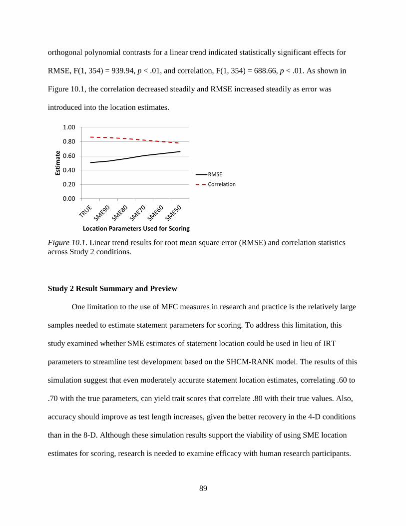
89
orthogonal polynomial contrasts for a linear trend indicated statistically significant effects for
RMSE, F(1, 354) = 939.94, p < .01, and correlation, F(1, 354) = 688.66, p < .01. As shown in
Figure 10.1, the correlation decreased steadily and RMSE increased steadily as error was
introduced into the location estimates.
Figure 10.1. Linear trend results for root mean square error (RMSE) and correlation statistics across Study 2 conditions.
Study 2 Result Summary and Preview
One limitation to the use of MFC measures in research and practice is the relatively large
samples needed to estimate statement parameters for scoring. To address this limitation, this
study examined whether SME estimates of statement location could be used in lieu of IRT
parameters to streamline test development based on the SHCM-RANK model. The results of this
simulation suggest that even moderately accurate statement location estimates, correlating .60 to
.70 with the true parameters, can yield trait scores that correlate .80 with their true values. Also,
accuracy should improve as test length increases, given the better recovery in the 4-D conditions
than in the 8-D. Although these simulation results support the viability of using SME location
estimates for scoring, research is needed to examine efficacy with human research participants.
0.00
0.20
0.40
0.60
0.80
1.00
Estim
ate
Location Parameters Used for Scoring
RMSE
Correlation

90
Study 3 was designed to initiate work in that domain, as a prelude to a more comprehensive
future investigation.

91
CHAPTER 11
STUDY 3:
A CONSTRUCT VALIDITY INVESTIGATION OF SHCM-RANK SCORES
The simulation studies in previous chapters examined the efficacy of the MCMC
algorithms for recovering HCM-RANK and SHCM-RANK item and person parameters.
Such simulation work is essential for refining algorithms, developing evidence-based guidelines
for test construction, and making projections about reliability of MFC tests in field applications.
However, empirical research is ultimately needed to provide an external check on the validity of
those inferences.
This chapter describes a small construct validity study to complement the simulation
findings. It was intended only to provide a stepping stone for future validity investigations. In a
nutshell, I examined the convergent and discriminant validities of four single-statement
personality measures and a 4-D MFC tetrad measure that was scored three ways, and the
relationships of the scores with external criteria. The correlations between the Likert-type sum
scores for the respective single-statement measures and the MCMC-based scores for the tetrad
measure serve as indicators of convergent validity, and the cross-dimension correlations serve as
indicators of discriminant validity. Finally, the correlation between the dimension scores for each
approach and related outcome variables provide additional indications of the efficacy of the
MFC tetrad methods.
92
Participants and Measures
The empirical sample consisted of 253 individuals who anonymously completed an
online personality questionnaire as part of a larger data collection project (Loo, manuscript in
progress) and three SMEs who were asked to estimate the locations of the personality statements
included in that questionnaire. It was expected that three SMEs would be sufficient for this
purpose, given that Stark et al. (2011) used just two and found that trait scores based on the SME
judgments correlated above .9 with trait scores based on marginal maximum likelihood
estimates; and their Study 2 found only a marginal decrease in person parameter recovery as
SME rating error increased.
The online participants responded to a personality questionnaire involving single-
statement items and tetrads measuring four broad personality factors: extraversion, openness to
experience, conscientiousness, and emotional stability. The 12-item single-statement measures of
each factor were created by selecting statements from the International Personality Item Pool
(IPIP; Goldberg et al., 2006). This single-statement measure is presented in Appendix C.
Participants indicated their level of agreement with each statement on a 1 (strongly disagree) to 4
(strongly agree) scale. The 4-D MFC measure was created by rearranging the 48 personality
statements used in Study 1 into 12 tetrads, which respondents ranked from 1 (most like me) to 4
(least like me). An effort was made to balance the social desirability of the statements within
each tetrad and, in the aggregate, to include statements that spanned the trait continua from low
to high. This tetrad measure is presented in Appendix D.
The SME estimates of statement locations were obtained in the manner described by
Stark et al. (2011). The SMEs for this study were three individuals with postgraduate degrees in
Industrial-Organizational Psychology and experience with item writing and the personality
93
constructs of interest. The 48 personality statements measuring 4 dimensions were shuffled and
presented to three SMEs with instructions to consider each statement independently and indicate
its standing on the trait continuum using a 1 (very low) to 7 (very high) scale. The ratings were
then averaged across SMEs and transformed to a -3.0 to 3.0 scale for SHCM-RANK scoring.
To examine the relationship of the personality scores to external criteria, information on
participants’ organizational citizenship (OCB) and counterproductive work behaviors (CWB)
were gathered using both self-report responses and coworker ratings. Because self-report OCB
and CWB scores may be contaminated by biases similar to those that distort personality scores,
coworker ratings for 170 of the participants were examined as a secondary source of participants’
behaviors. OCB was assessed using a 10-item measure of personal OCB (“Went out of the way
to give coworker encouragement or express appreciation”; α = .78) from a checklist developed
by Fox, Spector, Goh, Bruurseman, and Kessler (2012). Participants and coworkers responded to
this measure using a five-point Likert-type format on a 1 (never) to 5 (every day) scale.
Participant CWB (“Stolen something belonging to your employer”; α = .95) was measured using
Spector et al.’s (2006) 32-item Counterproductive Work Behavior Checklist. Participants
responded to this measure by indicating how often they have done a series of behaviors on their
job. Responses were gathers using a five-point Likert-type format on a 1 (never) to 5 (every day)
scale.
Although a recent meta-analysis found a significant relationship for emotional stability (r
= -.20) and conscientiousness (r = -.19) with self-report CWB (Berry, Ones, & Sackett, 2007),
the use of observer-report CWB indicates very little relationship with emotional stability (r = -
.04) (Berry, Carpenter, & Barratt, 2012). Similarly, meta-analytic results indicate that self-report
emotional stability (r = .10), conscientiousness (r = .14), and openness (r = .11) scores

94
moderately relate to OCB (Chiaburu, Oh, Berry, Li, & Gardner, 2011), but studies involving
observer-report OCB indicate a significant relationship only for conscientiousness (r = .13)
(Bourdage, Lee, Lee, & Shin, 2012; Connelly & Hülsheger, 2012). Collectively, these findings
suggest that using self-report Likert-type measures of predictor and criterion variables may
inflate the relationships of interest, so research is needed to see whether MFC measures will be
more resistant to potential response sets.
Analyses
Personality scores for the 253 online participants were calculated four ways. The four
single-statement measures were scored by reverse coding negatively worded statements and
summing the selected category codes to obtain LIKERT trait scores for each participant. Then
the MFC tetrad rank responses were scored three ways:
1) HCM-RANK trait scores were obtained by directly (simultaneously) estimating item and
person parameters from the rank responses;
2) SHCM-RANK trait scores were obtained by directly (simultaneously) estimating item
and person parameters from the rank responses; and
3) SHCM-RANK-SME trait scores were obtained by scoring the rank responses using SME
location estimates.
Finally, scale scores for the OCB and CWB measures were calculated through the traditional
approach of reverse coding negatively worded statements and summing across the items
composing each measure.
The correlations between these sets of scores were used to examine convergent and
discriminant validity. High correlation between the respective LIKERT and HCM-RANK trait
scores provides support for the new IRT model and its MCMC implementation. High correlation
95
between those scores and the SHCM-RANK scores signifies that the simpler one-parameter
model should be carefully considered for future field applications. High correlations between the
previous sets of scores and the SHCM-RANK-SME scores provides evidence that SME location
estimates can be also used to streamline multidimensional forced choice test development,
supporting Stark et al.’s (2011) findings for unidimensional forced choice tests. Lower
intercorrelations among the dimensions assessed with tetrads signals better discriminant
validities, perhaps due to reduced social desirability response bias. Finally, similar correlations
between LIKERT, HCM-RANK, SHCM-RANK, and SHCM-RANK-SME scores and related
outcome measures indicates that trait recovery is comparable across MFC strategies when
compared to a traditional Likert approach, providing evidence of the validity of those scores.
Hypotheses
Chernyshenko et al. (2009) demonstrated that IRT-based multidimensional pairwise
preference, unidimensional pairwise preference, and single-statement personality tests
administered under “honest” conditions have similar convergent, discriminant, and predictive
validities. In addition, Stark et al. (2011) showed that trait scores for unidimensional pairwise
preference tests are fairly robust to error in statement parameter estimates stemming from
calibrating small samples or substituting SME estimates of statement locations. With these
findings in mind, the following hypotheses were proposed:
1. Comparing HCM-RANK, SHCM-RANK, and SHCM-RANK-SME trait scores: The
monotrait heteromethod correlations will be high, and similar heterotrait monomethod
correlations will be observed across the approaches.
2. The monotrait heteromethod correlations between the LIKERT trait scores and HCM-
RANK, SHCM-RANK, and SHCM-RANK-SME trait scores will be high.
96
3. The heterotrait monomethod correlations for LIKERT trait scores will be higher than
those for the HCM-RANK, SHCM-RANK, and SHCM-RANK-SME approaches.
4. Examining the criterion measures, personality scores for both LIKERT and MFC tetrad
scoring will show moderate correlations with self-report OCB and CWB scores, and
small correlations with coworker-report OCB and CWB scores.
As the HCM-RANK, SHCM-RANK, and SHCM-RANK-SME approaches score the same
response data using different methods, the hypotheses offered here were examined through the
creation and inspection of a multi-trait multi-method matrix of correlations. Additionally, the
correlations between the personality scores and the criterion scores were compared across
formats to examine their comparability.
97
CHAPTER 12:
STUDY 3 RESULTS
This study was conducted as initial foray into HCM-RANK and SHCM-RANK MFC test
construction and scoring with human research participants. Table 12.1 presents the multi-trait
multi-method matrix for emotional stability, conscientiousness, openness, and extraversion
obtained using single-statement measures and MFC item tetrads that were scored using three
approaches. The bold values along the diagonals of each scoring format highlight the monotrait
hetromethod correlations. As can be seen in the table, these correlations were generally large,
with values ranging from .60 to .94. The correlations among trait scores were lowest for the
SHCM-RANK and SHCM-RANK-SME methods. Overall, the high monotrait heteromethod
correlations support the first part of Hypothesis 1.
In Table 12.1, it can be seen that the correlations between LIKERT and MFC scores were
highest for emotional stability and extraversion and lowest for conscientiousness and openness.
However, the correlations were low overall, ranging from just .26 to .61, which does not support
Hypothesis 2 concerning convergent validity.
Given this finding, it is important to consider potential explanations. One explanation is
that the statements measuring each construct were too different across measures, so different
facets or aspects of personality may have been emphasized. For example, Heggestad et al. (2006)
found correlations ranging from .75 to .87 between MFC tetrads and single-statement measures
when items had overlapping content, but the correlations decreased to a range of .58 to .71 when
98
overlap was eliminated. Similarly, Chernyshenko et al. (2009) found correlations across formats
ranging from .54 to .75 with a modest degree of overlap.
A second possible explanation for the low convergent validity is the LIKERT measures
were more influenced by response distortion than the MFC measure, and the MFC measure
yielded more accurate trait scores. Of course, an alternative explanation is that the MFC scores
were inaccurately estimated because the measure was too short to provide sufficient test
information, or the examinees found it more difficult and responded haphazardly. It is also
possible that all of these explanations are relevant to some extent.
Turning to the heterotrait monomethod correlations in Table 12.1, it can be seen that
there is some inconsistency in the relationship among the personality dimensions across the
HCM-RANK, SHCM-RANK, and SHCM-RANK-SME strategies. Both the HCM-RANK and
the SHCM-RANK-SME scores showed significant correlations between emotional stability and
openness, while SHCM-RANK estimates did not. Similarly, both SHCM-RANK and SHCM-
RANK-SME scores showed significant correlations between openness and extraversion, but in
the opposite direction. Consequently, the consistency of heterotrait monomethod correlations
proposed in Hypothesis 1 was not supported. The heterotrait monomethod correlations were,
however, larger for LIKERT scores when compared to the MFC tetrad scores, indicating some
ability for the forced choice models to reduce score inflation commonly found in self-report
measures. This pattern of results supports Hypothesis 3.
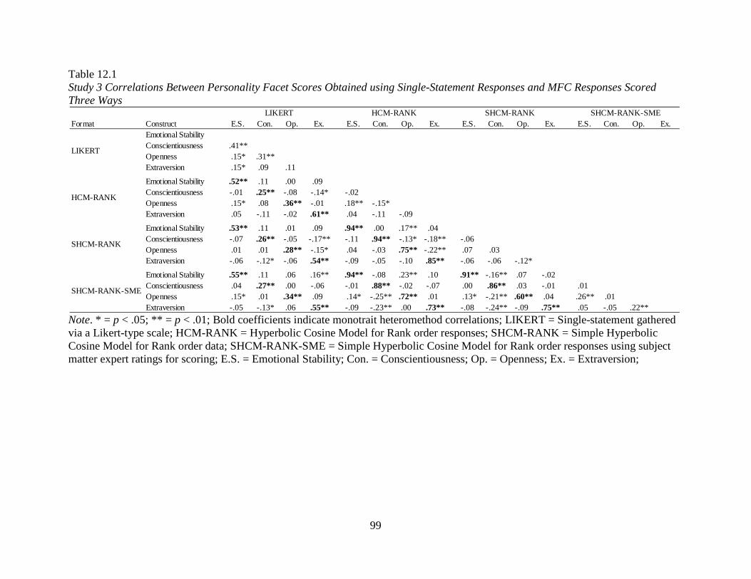
99
Table 12.1 Study 3 Correlations Between Personality Facet Scores Obtained using Single-Statement Responses and MFC Responses Scored Three Ways
Note. * = p < .05; ** = p < .01; Bold coefficients indicate monotrait heteromethod correlations; LIKERT = Single-statement gathered via a Likert-type scale; HCM-RANK = Hyperbolic Cosine Model for Rank order responses; SHCM-RANK = Simple Hyperbolic Cosine Model for Rank order data; SHCM-RANK-SME = Simple Hyperbolic Cosine Model for Rank order responses using subject matter expert ratings for scoring; E.S. = Emotional Stability; Con. = Conscientiousness; Op. = Openness; Ex. = Extraversion;
Format Construct E.S. Con. Op. Ex. E.S. Con. Op. Ex. E.S. Con. Op. Ex. E.S. Con. Op. Ex.Emotional StabilityConscientiousness .41**Openness .15* .31**Extraversion .15* .09 .11
Emotional Stability .52** .11 .00 .09 Conscientiousness -.01 .25** -.08 -.14* -.02 Openness .15* .08 .36** -.01 .18** -.15*Extraversion .05 -.11 -.02 .61** .04 -.11 -.09
Emotional Stability .53** .11 .01 .09 .94** .00 .17** .04 Conscientiousness -.07 .26** -.05 -.17** -.11 .94** -.13* -.18** -.06 Openness .01 .01 .28** -.15* .04 -.03 .75** -.22** .07 .03 Extraversion -.06 -.12* -.06 .54** -.09 -.05 -.10 .85** -.06 -.06 -.12*
Emotional Stability .55** .11 .06 .16** .94** -.08 .23** .10 .91** -.16** .07 -.02 Conscientiousness .04 .27** .00 -.06 -.01 .88** -.02 -.07 .00 .86** .03 -.01 .01 Openness .15* .01 .34** .09 .14* -.25** .72** .01 .13* -.21** .60** .04 .26** .01 Extraversion -.05 -.13* .06 .55** -.09 -.23** .00 .73** -.08 -.24** -.09 .75** .05 -.05 .22**
SHCM-RANK-SME
LIKERT HCM-RANK SHCM-RANK SHCM-RANK-SME
LIKERT
HCM-RANK
SHCM-RANK
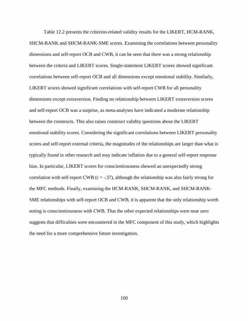
100
Table 12.2 presents the criterion-related validity results for the LIKERT, HCM-RANK,
SHCM-RANK and SHCM-RANK-SME scores. Examining the correlations between personality
dimensions and self-report OCB and CWB, it can be seen that there was a strong relationship
between the criteria and LIKERT scores. Single-statement LIKERT scores showed significant
correlations between self-report OCB and all dimensions except emotional stability. Similarly,
LIKERT scores showed significant correlations with self-report CWB for all personality
dimensions except extraversion. Finding no relationship between LIKERT extraversion scores
and self-report OCB was a surprise, as meta-analyses have indicated a moderate relationship
between the constructs. This also raises construct validity questions about the LIKERT
emotional stability scores. Considering the significant correlations between LIKERT personality
scores and self-report external criteria, the magnitudes of the relationships are larger than what is
typically found in other research and may indicate inflation due to a general self-report response
bias. In particular, LIKERT scores for conscientiousness showed an unexpectedly strong
correlation with self-report CWB (r = -.37), although the relationship was also fairly strong for
the MFC methods. Finally, examining the HCM-RANK, SHCM-RANK, and SHCM-RANK-
SME relationships with self-report OCB and CWB, it is apparent that the only relationship worth
noting is conscientiousness with CWB. That the other expected relationships were near zero
suggests that difficulties were encountered in the MFC component of this study, which highlights
the need for a more comprehensive future investigation.
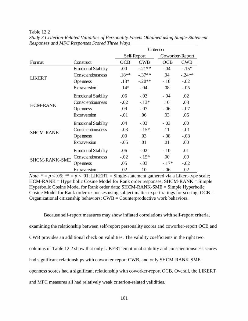
101
Table 12.2 Study 3 Criterion-Related Validities of Personality Facets Obtained using Single-Statement Responses and MFC Responses Scored Three Ways
Note. * = p < .05; ** = p < .01; LIKERT = Single-statement gathered via a Likert-type scale; HCM-RANK = Hyperbolic Cosine Model for Rank order responses; SHCM-RANK = Simple Hyperbolic Cosine Model for Rank order data; SHCM-RANK-SME = Simple Hyperbolic Cosine Model for Rank order responses using subject matter expert ratings for scoring; OCB = Organizational citizenship behaviors; CWB = Counterproductive work behaviors.
Because self-report measures may show inflated correlations with self-report criteria,
examining the relationship between self-report personality scores and coworker-report OCB and
CWB provides an additional check on validities. The validity coefficients in the right two
columns of Table 12.2 show that only LIKERT emotional stability and conscientiousness scores
had significant relationships with coworker-report CWB, and only SHCM-RANK-SME
openness scores had a significant relationship with coworker-report OCB. Overall, the LIKERT
and MFC measures all had relatively weak criterion-related validities.
Format Construct OCB CWB OCB CWBEmotional Stability .00 -.21** -.04 -.15*Conscientiousness .18** -.37** .04 -.24**Openness .13* -.20** -.10 -.02 Extraversion .14* -.04 .08 -.05
Emotional Stability .06 -.03 -.04 .02 Conscientiousness -.02 -.13* .10 .03 Openness .09 -.07 -.06 -.07 Extraversion -.01 .06 .03 .06
Emotional Stability .04 -.03 -.03 .00 Conscientiousness -.03 -.15* .11 -.01 Openness .00 .03 -.08 -.08 Extraversion -.05 .01 .01 .00
Emotional Stability .06 -.02 -.10 .01 Conscientiousness -.02 -.15* .00 .00 Openness .05 -.03 -.17* -.02 Extraversion .02 .10 -.06 .02
Criterion
LIKERT
HCM-RANK
SHCM-RANK
SHCM-RANK-SME
Self-Report Coworker-Report

102
Study 3 Results Summary
Chapters 11 and 12 describe a small validity study that took an initial look at HCM-
RANK MFC testing with human research participants. This study utilized an existing dataset to
examine the convergent and discriminant validities of MFC tetrad scores, relative to traditional
Likert-type scores, as well as relationships with external criteria. Overall, the results did not
provide clear support for the construct validity of the HCM-RANK, SHCM-RANK, or SHCM-
RANK-SME scores, but several possible explanations were offered for the unexpected findings.
To prevent similar problems in future studies, researchers are encouraged to carefully pretest
item tetrads, explore methods to compute MFC test information, and carefully pretest MFC
measures using simulations to insure that test length is adequate for trait estimation.
103
Chapter 13:
DISCUSSION AND CONCLUSIONS
Although there has been an increased interest in the assessment of noncognitive
constructs in educational and organizational settings, concerns surrounding the influence of
response bias and response styles on these measures have limited their application in a wide
range of settings. To address these concerns, researchers have examined alternative item
presentation formats that may provide resistance to such biases. One such format is a
multidimensional forced-choice item, which requires respondents to rank statements representing
different dimensions in terms of preference, or alternatively to provide most like and/or least like
responses. Several recent studies suggests that multidimensional forced choice measures reduce
response biases and sets while providing normative information that can be used for decision
making (Brown & Maydeu-Olivares, 2012; Heggestad, Morrison, Reeve, & McCloy., 2006;
Stark, Chernyshenko, Drasgow, & White, 2012).
The purpose of this dissertation was to develop a new IRT model that can be applied to a
variety of MFC item types. After deriving equations for the HCM-PICK and SHCM-PICK
models for most like choices among a number of options, the HCM-RANK and SHCM-RANK
models were developed based on the PICK probabilities. MCMC estimation algorithms were
then developed for statement and person parameters, and a Monte Carlo simulation was
performed to examine the efficacy of parameter recovery with direct and two-stage estimation
approaches. The results indicated reasonable recovery of person parameters and excellent
recovery of statement location parameters.
104
Follow-up studies were conducted to examine the potential for using SME estimates of
statement locations for scoring, as well as the validity of MFC HCM-RANK methods with
human research participants. The SME study indicated that location estimates can be used as
proxies for IRT estimates in the early stages of MFC test development. However, more research
is needed to look into difficulties that were encountered in the validity investigation.
Despite this, one motivation for the use of MFC items is to reduce the response biases
and response styles evidenced in applied and cross-cultural studies. The construction of MFC
item tetrads utilized for this dissertation balanced the social desirability of the constituent
statements, reflecting a process intended to reduce item transparency and, presumably, response
bias. Consequently, it is expected that the models presented here will provide the basis for
empirically demonstrating this reduction in response bias in future studies.
Future Research
The direct estimation of statement parameters from MFC responses provides an
opportunity to better understand how statements are evaluated within a context. This
understanding will assist in the creation of parallel test forms, which are necessary for high-
stakes uses. Additionally, direct estimation facilitates comparisons of item properties across
subgroups, which is important in cross-cultural research and incumbent in some high stakes
settings. Indeed, the SIOP Principles and Testing Standards (American Educational Research
Association, American Psychological Association, & National Council on Measurement in
Education, 1999) indicate that differential item functioning (DIF) analyses should be conducted
when possible to promote bias-free measurement. Current strategies for detecting DIF with MFC
items focus primarily on individual statements during item precalibration, but direct estimation
105
paves the way for comparisons of statement properties, for example, in the context of pairs and
tetrads that have already been administered for assessment purposes.
Future research is also needed to develop a strategy for examining item and test
information provided by the models described here. The derivation of information functions for
the HCM-RANK and SHCM-RANK models may be particularly difficult as the complete
response probability is based on a sequence of decisions where, in the case of a tetrad, there are
24 possible rankings. Instead, considering the information provided by an MFC item at the first
most like selection using the HCM-PICK and SHCM-PICK may provide a more tractable avenue
for developing item and test information functions. Estimation of the information provided by
test items across each of the dimensions being assessed would be advantageous for test
construction and evaluating the relative performance of different measures. Comparing the
information provided by the Likert-type scales and the MFC measure in Study 3 would help
determine whether the weak correlation resulted primarily from MFC measurement error.
Although Study 3 used a personality measure to illustrate the new MFC techniques, the
methods developed in this dissertation offer interesting possibilities for situational judgment test
(SJT) development and scoring. SJT items consist of scenarios followed by blocks of statements
that represent different dimensions. Examinees are typically asked to indicate what they
should/would do by choosing the best/most likely option or by ranking options from best/most
likely to worst/least likely. Scores are typically obtained through a classical test theory approach
involving SME estimates of statement effectiveness (i.e. location). Consequently, the HCM-
PICK and HCM-RANK, as well as the corresponding SHCM, models may be useful for
examining item quality, scoring, and constructing parallel forms.

106
Finally, although MFC methods have been discussed throughout this manuscript as a way
of improving the quality of self-report data in noncognitive assessment, they can certainly be
used for collecting observer reports for an equally large array of constructs. Borman et al. (2001)
found that unidimensional forced choice measures reduced a variety of rater errors in the context
of performance appraisal, so there is reason to believe that the MFC methods would also be
effective, and researchers are encouraged to avidly explore these possibilities. The models
presented here provide a basis for exploring these prospects in future research.
107
REFERENCES
Albert, J. H. (1992). Bayesian estimation of normal ogive item response curves using Gibbs
Sampling. Journal of Educational Statistics, 17(3), 251-269.
American Educational Research Association, American Psychological Association, and the
National Council on Measurement in Education (1999). Standards for educational and
psychological testing. Washington , DC : American Educational Research Association.
Andrich, D. (1982). An extension of the Rasch model for ratings providing both location and
dispersion parameters. Psychometrika, 47, 105-113.
Andrich, D. (1995). Hyperbolic cosine latent trait models for unfolding direct responses and
pairwise preferences. Applied Psychological Measurement, 19(3), 269-290.
Andrich, D. (1996). A hyperbolic cosine latent trait model for unfolding polytomous responses:
Reconciling Thurstone and Likert methodologies. British Journal of Mathematical
Statistical Psychology, 49, 347-365.
Andrich, D. & Luo, G. (1993). A hyperbolic cosine latent trait model for unfolding dichotomous
single-stimulus responses. Applied Psychological Measurement, 17, 253-276.
Andrich, D., & Luo, G. (1996). RUMMFOLDss: A Windows program for analyzing single
stimulus responses of persons to items according to the hyperbolic cosine unfolding
model. [Computer program]. Perth, Australia: Murdoch University.
Baker, B. B., & Kim, S. (2004). Item Response Theory Parameter Estimation Techniques, (2nd
Ed.). Boca Raton, FL: Taylor & Francis Group.
108
Baron, H. (1996). Strengths and limitations of ipsative measurement. Journal of Occupational
and Organizational Psychology, 69, 49-56.
Bartram, D. (2007). Increasing validity with forced-choice criterion measurement formats.
International Journal of Selection and Assessment, 15(3), 263-272.
Berry, C. M., Carpenter, N. C., & Barratt, C. L. (2012). Do other-reports of counterproductive
work behavior provide an incremental contribution over self-reports? A meta-analytic
comparison. Journal of Applied Psychology, 97(3), 613-636.
Berry, C. M., Ones, D. S., & Sackett, P. R. (2007). Interpersonal deviance, organizational
deviance, and their common correlates: A review and meta-analysis. Journal of Applied
Psychology, 92(2), 410-424.
Birnbaum, A. (1968). Some latent trait models and their use in inferring an examinee’s ability. In
F. M. Lord & M. R. Novick (Eds.), Statistical theories of mental test scores. (pp. 397-
472). Reading, MA: Addison-Wesley.
Bock, R. D. (1972). Estimating item parameters and latent ability when responses are scored in
two or more nominal categories. Psychometrika, 37, 29-51.
Bock,R. D.,& Aitkin,M. (1981). Marginal maximum likelihood estimation of item parameters:
Application of an EM algorithm. Psychometrika, 46, 443-459.
Böckenholt, U. (2001). Hierarchical modeling of paired comparison data. Psychological
Methods, 6, 49–66.
Böckenholt, U. (2004). Comparative judgments as an alternative to ratings: Identifying the scale
origin. Psychological Methods, 9, 453–465.
109
Bourdage, J. S., Lee, K., Lee, J., & Shin, K. (2012). Motives for organizational citizenship
behavior: Personality correlates and coworker ratings of OCB. Human Performance, 25,
179-200.
Borman, W. C. (2004). The concept of organizational citizenship. Current Directions in
Psychological Science, 13(6), 238-241.
Borman, W. C. & Motowidlo, S. J. (1997). Task performance and contextual performance: The
meaning for personnel selection research. Human Performance, 10, 99-109.
Borman, W. C., Buck, D. E., Hanson, M. A., Motowidlo, S. J., Stark, S., & Drasgow, F. (2001).
An examination of the comparative, reliability, validity, and accuracy of performance
ratings made using computerized adaptive rating scales. Journal of Applied Psychology,
86, 965-973.
Brown, A. (2010). How IRT can solve problems of ipsative data (Doctoral dissertation).
University of Barcelona, Spain.
Brown, A., & Maydeu-Olivares, A. (2011). Item response modeling of forced-choice
questionnaires. Educational and Psychological Measurement, 71(3). 460-502.
Brown, A., & Maydeu-Olivares, A. (2012). Fitting a Thurstonian IRT model to forced-choice
data using Mplus. Behavior Research Methods, 44(4), 1135-1147.
Brown, A., & Maydeu-Olivares, A. (2013). How IRT Can Solve Problems of Ipsative Data in
Forced-Choice Questionnaires. Psychological Methods, 18(1), 36-52.
Campbell, J. P. (1990). Modeling the performance prediction problem in industrial and
organizational psychology. In M. Dunnette & L. M. Hough (Eds.), Handbook of
industrial and organizational psychology (pp. 687-731). Palo Alto, CA: Consulting
Psychologists Press.
110
Carter, N. T., & Dalal, D. K. (2010). An ideal point account of the JDI work satisfaction scale.
Personality and Individual Differences, 49, 743-748.
Carter, N. T., & Zickar, M. J. (2011a). The influence of dimensionality on parameter estimation
accuracy in the generalized graded unfolding model. Educational and Psychological
Measurement, 71, 765-788.
Carter, N.T., & Zickar, M.J. (2011b). A comparison of the LR and DFIT frameworks of
differential functioning applied to the generalized graded unfolding model. Applied
Psychological Measurement, 35, 623-642.
Cattell, R. B., & Cattell, H. P. (1995). Personality structure and the new fifth edition of the 16PF.
Educational and Psychological Measurement,55, 926–937.
Chernyshenko, O.S., Stark, S., Drasgow, F., & Roberts, B.W. (2007). Constructing personality
scales under the assumptions of an ideal point response process: Toward increasing the
flexibility of personality measures. Psychological Assessment, 19(1), 88-106.
Chernyshenko, O. S., Stark, S., Prewett, M. S., Gray, A. A., Stilson, F. R., & Tuttle, M.D.
(2009). Normative scoring of multidimensional pairwise preference personality scales
using IRT: Empirical comparison with other formats. Human Performance, 22, 105-127.
Cheung, G. W., & Rensvold, R. B. (2000). Assessing extreme and acquiescence response sets in
cross-cultural research using structural equations modeling. Journal of Cross-Cultural
Psychology, 13(2), 187-212.
Chiaburu, D. S., Oh, I., Berry, C. M., Li, N., & Gardner, R. G. (2011). The five-factor model of
personality traits and organizational citizenship behaviors: A meta-analysis. Journal of
Applied Psychology, 96(6), 1140-1166.
111
Christiansen, N. D., Burns, G. N., & Montgomery, G. E. (2005). Reconsidering forced-choice
item formats for applicant personality assessment. Human Performance, 18(3), 267-307.
Christiansen, N. D., Goffin, R. D., Johnson, N. G., & Rothstein, M. G. (1994). Correcting the
16PF for faking: Effects on criterion-related validity and individual hiring decisions.
Personnel Psychology, 47(4), 847-860.
Critchlow, D. E., Fligner, M. A., & Verducci, J. S. (1991). Probability models on rankings.
Journal of Mathematical Psychology, 35(3), 294-318.
Connelly, B. S., & Hülsheger, U. R. (2012). A narrower scope or a clearer lens for personality?
Examining sources of observers’ advantages over self-reports for predicting performance.
Journal of Personality, 80(3), 603-631.
Converse, P. D., Oswald, F. L., Imus, A., Hedricks, C., Roy, R., & Butera, H. (2008). Comparing
personality test formats and warnings: Effects on criterion-related validity and test-taker
reactions. International Journal of Selection and Assessment, 26(2), 155-169.
Coombs, C. H. (1964). A theory of data. New York, NY: Wiley.
de la Torre, J., Ponsoda, V., Leenen, I., & Hontangas, P. (2012, April). Examining the viability of
recent models for forced-choice data. Presented at the Meeting of the American
Educational Research Association, Vancouver, British Columbia, Canada.
DeSarbo, W. W., de Soete, G., Eliashberg, J. (1987). Journal of Economic Psychology, 8(3),
357-384.
Diener, E., & Diener, M. (2009). Cross-cultural correlates of life satisfaction and self-esteem. In
Diener, E. (Ed)., Culture and well-being: The collected works of Ed Diener (pp. 71-91).
New York, NY: Springer Science & Business Media.
112
Doornik, J. A. (2009). An object-oriented matrix language: Ox 6. London, UK: Timberlake
Consultants Press.
Drasgow, F., Lee, W. C., Stark, S., & Chernyshenko, O. S. (2004). Alternative scoring
methodologies for predicting attrition in the army: The new AIM scales. In D. J. Knapp,
E. D. Heggestad, M. C. & Young (Eds.), Understanding and Improving the Assessment of
Individual Motivation (AIM) in the Army’s GED Plus Program (Army Research Institute
Report No. 2004-03; pp. 7.1-7.14).
Drasgow, F., Stark, S., & Chernyshenko, O.S. (2011, April). Tailored Adaptive Personality
Assessment System (TAPAS) prediction of soldier performance. Paper presented at the
26th annual conference for the Society of Industrial and Organizational Psychology.
Chicago, IL.
Drasgow, F., Stark, S, Chernyshenko, O. S., Nye, C. D., Hulin, C. L., & White, L. A. (2012).
Development of the tailored adaptive personality assessment system (TAPAS) to support
Army selection and classification decisions. Technical report. U.S. Army Research
Institute for the Behavioral and Social Sciences. Fort Belvoir, VA.
Fischer, R. (2004). Standardization to account for cross-cultural response bias: A classification
of score adjustment procedures and review of research in JCCP. Journal of Cross-
Cultural Psychology, 35(3), 263-282.
Fox, S., Spector, P. E., Goh, A., Bruursema, K., & Kessler, S. R. (2012). The deviant citizen.
Measuring potential positive relations between counterproductive work behavior and
organizational citizenship behavior. Journal of Occupational and Organizational
Psychology, 85(1), 199-220.
113
Frenzel., A. C., Thrash, T. M., Pekrun, R., & Goetz, T. (2007). Achievement emotions in
Germany and China: A cross-cultural validation of the Academic Emotions
Questionnaire-Mathematics. Journal of Cross-Cultural Psychology, 38(3), 302-309.
Goldberg, L. R. (1981). Language and individual differences: The search for universals in
personality lexicons. In L. Wheeler (Ed.), Review of personality and social psychology
(pp. 141-165). Beverly Hills, CA: Sage.
Goldberg, L. R., Johnson, J. A., Eber, H. W., Hogan, R., Ashton, M. C., Cloninger, C. R., &
Gough, H. C. (2006). The International Personality Item Pool and the future of public-
domain personality measures. Journal of Research in Personality, 40, 84-96.
Gordon, L. V. (1953). Gordon Personal Profile. Yonkers, New York: World Book.
Heggestad, E. D., Morrison, M., Reeve, C. L., & McCloy, R. A. (2006). Forced-choice
assessments of personality for selection: Evaluating issues of normative assessment and
faking resistance. Journal of Applied Psychology, 91(1), 9-24.
Hirsh, J. B., & Peterson, J. B. (2008). Predicting creativity and academic success with a “fake-
proof” measure of the big five. Journal of Research in Personality, 42, 1323-1333.
Hough, L., & Dilchert, S. (2010). Personality: Its measurement and validity for employee
selection. In J. L. Farr & N. T. Tippins (Eds.), Handbook of employee selection (pp. 299-
319). New York, NY, US: Routledge/Taylor & Francis Group.
Hulin, C. L., Drasgow, F., & Parsons, C. K. (1983). Item response theory: Applications to
psychological measurement. Homewood, IL: Dow Jones Irwin.
Jackson, D. N., Wroblewski, V. R., & Ashton, M. C. (2000). The impact of faking on
employment tests: Does forced choice offer a solution? Human Performance, 13(4), 371-
388.
114
Johnson, M. S., & Junker, B. W. (2003). Using data augmentation and Markov chain Monte
Carlos for the estimation of unfolding response models. Journal of Educational and
Behavioral Statistics, 28(3), 195-230.
Johnson, C. E., Wood, R., & Blinkhorn, S. F. (1988). Spuriouser and Spuriouser: The use of
ipsative personality tests. Journal of Occupational Psychology, 61(2), 153-162.
Kim, J. & Bolt, D. M. (2007). Estimating item response theory models using Markov chain
Monte Carlo methods. Educational Measurement: Issues and Practice, 26(4), 38-51.
Knapp, D. J., & Heffner, T. S. (2009). Validating future force performance measures (Army
class): End of training longitudinal validation. Technical report. U.S. Army Research
Institute for the Behavioral and Social Sciences. Arlington, VA.
Knapp, D. J., Heffner, T. S., & White, L. (2011). Tier one performance screen initial operational
test and evaluation: Early results. Technical report. U.S. Army Research Institute for the
Behavioral and Social Sciences. Arlington, VA.
Levine, M. V. (1984). An introduction to multilinear formula score theory. Measurement Series
No. 84–4. Office of Naval Research, Personnel and Training Research Programs.
Arlington, VA.
Likert, R. (1932). A technique for the measurement of attitudes. Archives of Personality, 140, 5-
53.
Loo, k. (manuscript in preparation). OCBs and Strain: The Moderating Role of Control (Doctoral
dissertation in progress). University of South Florida, Tampa, FL.
Lunn, D., Spiegelhalter, D., Thomas, A., Best, N. (2009). The BUGS project: Evolution, critique,
and future directions. Statistics in Medicine, 28, 3049-3067.
Luce, R. D. (1959). Individual choice behavior: A theoretical analysis. New York, NY: Wiley.
115
Luo, G. (2000). A joint maximum likelihood estimation procedure for the Hyperbolic Cosine
Model for single-stimulus responses. Applied Psychological Measurement, 24, 33-49.
Maydeu-Olivares, A. (2001). Limited information estimation and testing of Thurstonian models
for paired comparison data under multiple judgment sampling. Psychometrika, 66(2),
209-228.
Maydeu-Olivares, A., & Böckenholt, U. (2005). Structural equation modeling of paired-
comparison and ranking data. Psychological Methods, 10, 285–304.
Maydeu-Olivares, A., & Brown, A. (2010). Item response modeling of paired comparison and
ranking data. Multivariate Behavioral Research, 45, 935–974.
McCloy, R. A., Heggestad, E. D., & Reeve, C. L. (2005). A silk purse from the sow’s ear:
Retrieving normative information from multidimensional forced-choice items.
Organizational Research Methods, 8(2), 222-248.
McGrane, J. A. (2009). Unfolding the conceptualisation and measurement of ambivalent
attitudes (Doctoral dissertation). University of Sydney, Sydney, Australia.
McGrath, R. E., Mitchell, M., Kim, B. H., & Leaetta, H. (2010). Evidence for response bias as a
source of error variance in applied assessment. Psychological Bulletin, 136(3), 450-470.
Meade, A. W. (2004). Psychometric problems and issues involved with creating and using
ipsative measures for selection. Journal of Occupational and Organizational Psychology,
77, 531-552.
Murphy, K. R., Jako, R. A., & Anhalt, R. L. (1993). Nature and consequences of halo error: A
critical analysis. Journal of Applied Psychology, 78(2), 218-225.
Muthén, L. K., & Muthén, B. (1998-2007). Mplus 5. Los Angeles, CA: Muthén & Muthén.
116
O’Brien, E., & LaHuis, D. M. (2011). Do applicants and incumbents respond to personality
items similarly? A comparison of dominance and ideal point response models.
International Journal of Selection and Assessment, 19(2), 109-118.
Patz, R. J., & Junker, B. W. (1999a). A straightforward approach to Markov chain Monte Carlo
methods for item response models. Journal of Educational and Behavioral Statistics,
24(2), 146-178.
Patz, R. J., & Junker, B. W. (1999b). Applications and extensions of MCMC in IRT: Multiple
item types, missing data, and rated responses. Journal of Educational and Behavioral
Statistics, 24(4), 342-366.
Paulhus, D. L. (1991). Measurement and control of response bias. In J. P. Robinson, P. R.
Shaver, & L. S. Wrightsman (Eds.), Measures of personality and social psychological
attitudes (pp. 17-59). San Diego, CA: Academic Press.
Richardson, M., Abraham, C., & Bond, R. (2012). Psychological correlates of university
students’ academic performance: A systematic review and meta-analysis. Psychological
Bulletin, 138(2), 353-387.
Roberts, J. S., Donoghue, J. R., & Laughlin, J. E. (2000). A general item response theory model
for unfolding unidimensional polytomous responses. Applied Psychological
Measurement, 24(1), 3-32.
Roberts, J. S., Donoghue, J. R., & Laughlin, J. E. (2002). Characteristics of MML/EAP
parameter estimates in the Generalized Graded Unfolding Model. Applied Psychological
Measurement, 26, 192-207.
117
Roberts, J. S., & Laughlin, J. E. (1996). A unidimensional item response model for unfolding
responses from a graded disagree-agree response scale. Applied Psychological
Measurement, 20(3), 231-255.
Roberts, J. S., Laughlin, J. E., & Wedell, D. H. (1999). Validity issues in the Likert and
Thurstone approaches to attitude measurement. Educational and Psychological
Measurement, 59(2), 211-233.
Roberts, J. S., Rost, J., & Macready, G. B. (2009). MIXUM: An unfolding mixture model to
explore the latitude of acceptance concept in attitude measurement. In S. E. Embretson
(Ed.), Measuring psychological constructs : advances in model-based approaches (pp.
175-197). Washington, DC: American Psychological Association.
Roberts, J. S., & Thompson, V. M. (2011). Marginal maximum a posteriori item parameter
estimation for the Generalized Graded Unfolding Model. Applied Psychological
Measurement, 35(4), 259-279.
Rosse, J. G., Stecher, M. D., Miller, J. L., & Levin, R. A. (1998). The impact of response
distortion on preemployment personality testing and hiring. Journal of Applied
Psychology, 83(4), 634-644.
Sackett, P. R., Schmitt, N., Ellingson, J. E., & Kabin, M. B. (2001). Highstakes testing in
employment, credentialing, and higher education: Prospects in a post-affirmative action
world. American Psychologist, 56, 302-318.
Seybert, J., Stark, S., & Chernyshenko, O. S. (2013) Detecting DIF with ideal point models: A
comparison of area and parameter difference methods. Manuscript submitted for
publication.
118
Seybert, J., Stark, S., & Chun, S. (manuscript in preparation). Reexamining the Hyperbolic
Cosine Model. University of South Florida, Tampa, FL.
SHL. (2006). OPQ32: Technical manual. Thames Ditton, UK: SHL Group plc.
Spector, P. E., Fox, S., Penney, L. M., Bruursema, K., Goh, A., & Kessler, S. R. (2006). The
dimensionality of counterproductivity: Are all counterproductive behaviors created
equal? Journal of Vocational Behavior, 68(3), 446-460.
Stark, S. (2002). A new IRT approach to test construction and scoring designed to reduce the
effects of faking in personality assessment: The generalized graded unfolding model for
multi-unidimensional paired comparison responses (Doctoral dissertation). University of
Illinois at Urbana-Champaign. Urbana-Champaign, IL.
Stark, S. (2013). MODFIT 4.0: An Excel VBA program for examining model-data fit with
dichotomous and polytomous IRT models. Unpublished manuscript. University of South
Florida.
Stark, S., Chernyshenko, O. S., & Drasgow, F. (2005). An IRT approach to constructing and
scoring pairwise preference items involving stimuli on different dimensions: The multi-
unidimensional pairwise-preference model. Applied Psychological Measurement, 29(3),
3, 184-203.
Stark, S., Chernyshenko, O.S., & Drasgow, F. (2010, September). Update on Tailored Adaptive
Personality Assessment System (TAPAS): Results and ideas to meet the challenges of
high stakes testing. Paper presented at the 52nd annual conference of the International
Military Testing Association. Lucerne, Switzerland.
119
Stark, S., Chernyshenko, O. S., & Drasgow, F. (2011). Constructing fake-resistant personality
tests using item response theory. In M. Ziegler, C. MacCann, & R. Roberts (Eds.), New
perspectives on faking in personality assessment (pp. 214-239). London: Oxford
University Press.
Stark, S., Chernyshenko, O. S., Drasgow, F., & White, L. A. (2012). Adaptive testing with
multidimensional pairwise preference items: Improving the efficiency of personality and
other noncognitive assessments. Organizational Research Methods, 15(3), 463-487.
Stark, S., Chernyshenko, O.S., Drasgow, F., White, L.A., Heffner, T., & Hunter, A. (2008,
October). Using multidimensional pairwise preference personality tests in military
contexts: Development and evaluation of the TAPAS-95S. Paper presented at the 50th
annual conference of the International Military Testing Association. Amsterdam, NL.
Stark, S., Chernyshenko, O. S., & Guenole, N. (2011). Can subject matter experts’ ratings of
statement extremity be used to streamline the development of unidimensional pairwise
preference scales? Organizational Research Methods, 14(2), 256-278.
Stark, S., & Drasgow, F., & Chernyshenko, O. S. (2008, October). Update on the Tailored
Adaptive Personality Assessment System (TAPAS): The next generation of personality
assessment systems to support personnel selection and classification decisions. Presented
at the 50th annual conference of the International Military Testing Association,
Amsterdam, Netherlands.
Stark, S., Chernyshenko, O.S., Lee, W.C. & Drasgow, F. (2000, April). New insights in
personality measurement: Application of an ideal point IRT model. Paper presented at the
15th annual conference for the Society of Industrial and Organizational Psychology. New
Orleans, LA.
120
Stark, S., & Drasgow, F. (2002). An EM approach to parameter estimation for the Zinnes and
Griggs paired comparison IRT model. Applied Psychological Measurement, 26, 208-227.
Stewart, G. L., Darnold, T. C., Zimmerman, R. D., Parks, L., & Dustin, S. L. (2010). Exploring
how response distortion of personality measures affects individuals. Personality and
Individual Differences, 49(6), 622-628.
Strong, E. K. (1938). Vocational interest blank for men. Palo Alto, CA: Stanford University
Press.
Taras, V., Kirkman, B. L., Steel, P. (2010). Examining the impact of Culture's consequences: A
three-decade, multilevel, meta-analytic review of Hofstede's cultural value dimensions.
Journal of Applied Psychology, 95(3), 405-439.
Tay, L., Drasgow, F., Rounds, J., & Williams, B.A. (2009). Fitting measurement models to
vocational interest data: Are dominance models ideal? Journal of Applied Psychology,
94(5), 1287-1304.
Thurstone, L. L. (1927). Psychophysical analysis. American Journal of Psychology, 38, 368-389.
Tierney, L. (1994). Exploring posterior distributions with Markov chains. Annals of Statistics,
22, 117-130.
Touloumtzoglou, J. (1999). Resolving binary responses in the Visual Arts Attitude Scale with the
Hyperbolic Cosine Model. International Education Journal, 1(2), 94-116.
Van de gaer, E., Grisay, A., Schulz, W., & Gebhardt, E. (2012). The reference group effect: An
explanation of the paradoxical relationship between academic achievement and self-
confidence across countries. Journal of Cross-Cultural Psychology, 43(8), 1205-1228.
121
van Herk, H., Poortinga, Y. H., Verhallen, T. M. (2004). Response styles in rating scales:
Evidence of method bias in data from six EU countries. Journal of Cross-Cultural
Psychology, 35(3), 346-360.
Vasilopoulos, N. L., Cucina, J. M., Dyomina, N. V., Morewitz, C. L., & Reilly, R. R. (2006).
Forced-choice personality tests: A measure of personality and cognitive ability? Human
Performance, 19, 175–199.
Viswesvaran, C., Deller, J., & Ones, D. S. (2007). Personality measures in personnel selection:
Some new contributions. International Journal of Selection and Assessment, 15(3), 354-
358.
Weeks, A. M., & Meijer, R. R. (2008). Scaling response processes on personality items using
unfolding and dominance models. European Journal of Psychological Assessment, 24(1),
65-77.
White, L. A., & Young, M. C. (1998, April). Development and validation of the Assessment of
Individual Motivation (AIM). Paper presented at the Annual Meeting of the American
Psychological Association, San Francisco, CA.
Wilkins, J. L. M. (2004). Mathematics and science self-concept: An international investigation.
Journal of Experimental Education, 72(4), 331-346.
Wollack, J. A., Bolt, D. M., Cohen, A. S., & Lee, Y. (2002). Recovery of item parameters in the
Nominal Response Model: A comparison of marginal maximum likelihood estimation
and Markov chain Monte Carlo estimation. Applied Psychological Measurement, 26(3),
339-352.
Yellott, J. I. (1980). Generalized Thurstone models for ranking: Equivalence and reversibility.
Journal of Mathematical Psychology, 22, 48-69.
122
Yellott, J. I. (1997). Preference models and irreversibility. In A. A. J. Marley (Ed.), Choice,
decision and measurement (pp. 131-151). Mahwah, NJ: Lawrence Erlbaum Associates.
Young, M. C., McCloy, R. A., Waters, B. K., & White, L. A. (2004). An overview of AIM and
the preliminary efforts to support its operational use. In D. J. Knapp, E. D. Heggestad, M.
C. & Young (Eds.), Understanding and Improving the Assessment of Individual
Motivation (AIM) in the Army’s GED Plus Program (Army Research Institute Report No.
2004-03; pp. 1.1-1.11).
Zickar, M. J., Rosse, J. G., Levin, R. A., & Hulin, C. L. (1996, April). Modeling the effects of
faking on personality tests. Paper presented at the 11th annual meeting of the Society for
Industrial and Organizational Psychology, San Diego, CA.
Zinnes, J. L., & Griggs, R. A. (1974). Probabilistic, multidimensional unfolding analysis.
Psychometrika, 39, 327-350.
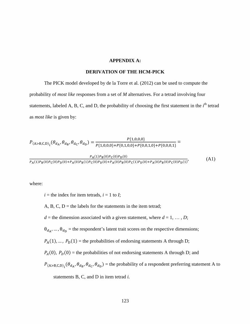
123
APPENDIX A:
DERIVATION OF THE HCM-PICK
The PICK model developed by de la Torre et al. (2012) can be used to compute the
probability of most like responses from a set of M alternatives. For a tetrad involving four
statements, labeled A, B, C, and D, the probability of choosing the first statement in the ith tetrad
as most like is given by:
𝑃(A>B,C,D)𝑖(𝜃𝑑A ,𝜃𝑑B ,𝜃𝑑C ,𝜃𝑑D) =
𝑃{1,0,0,0}𝑃{1,0,0,0}+𝑃{0,1,0,0}+𝑃{0,0,1,0}+𝑃{0,0,0,1}
=
𝑃A(1)𝑃B(0)𝑃C(0)𝑃D(0)𝑃A(1)𝑃B(0)𝑃C(0)𝑃D(0)+𝑃A(0)𝑃B(1)𝑃C(0)𝑃D(0)+𝑃A(0)𝑃B(0)𝑃C(1)𝑃D(0)+𝑃A(0)𝑃B(0)𝑃C(0)𝑃D(1), (A1)
where:
i = the index for item tetrads, i = 1 to I;
A, B, C, D = the labels for the statements in the item tetrad;
d = the dimension associated with a given statement, where d = 1, … , D;
θ𝑑A , … , θ𝑑D = the respondent’s latent trait scores on the respective dimensions;
𝑃A(1), … , 𝑃D(1) = the probabilities of endorsing statements A through D;
𝑃𝐴(0), 𝑃𝐷(0) = the probabilities of not endorsing statements A through D; and
𝑃(A>B,C,D)𝑖(𝜃𝑑A ,𝜃𝑑B ,𝜃𝑑C ,𝜃𝑑D) = the probability of a respondent preferring statement A to
statements B, C, and D in item tetrad i.
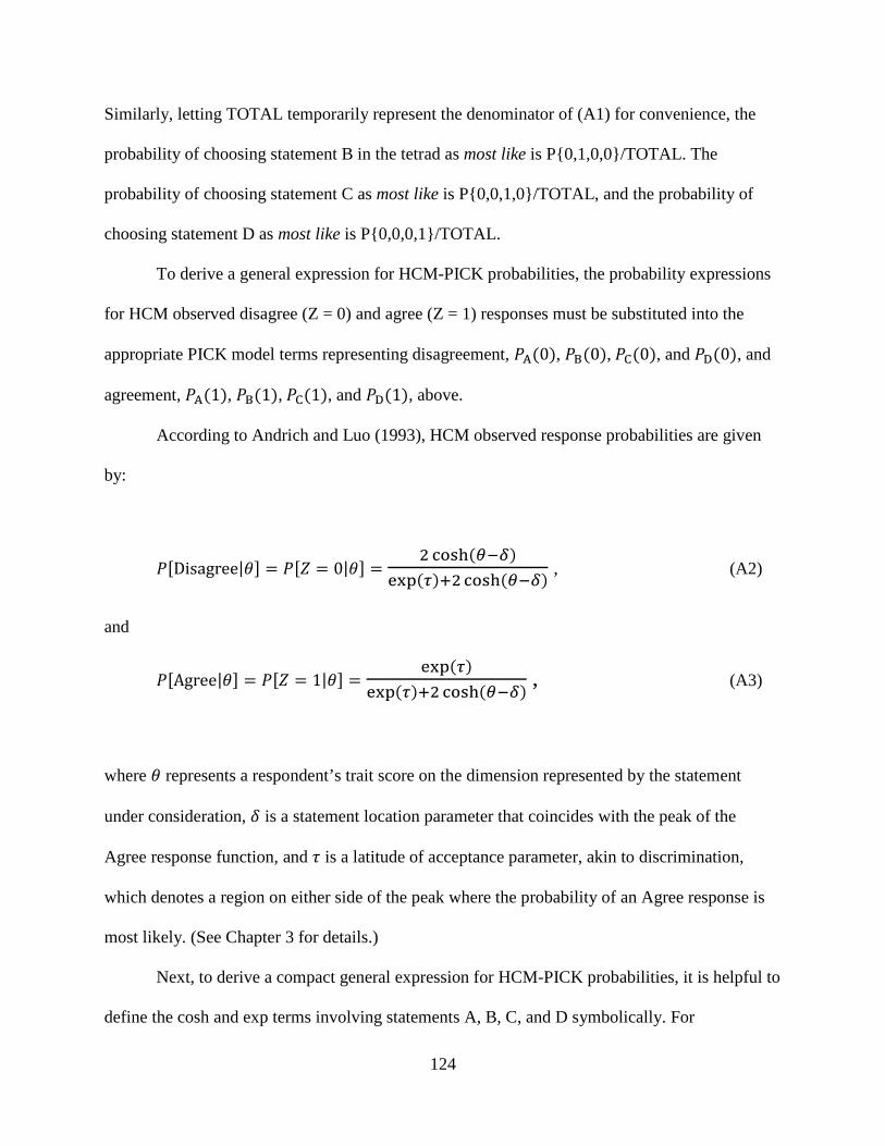
124
Similarly, letting TOTAL temporarily represent the denominator of (A1) for convenience, the
probability of choosing statement B in the tetrad as most like is P{0,1,0,0}/TOTAL. The
probability of choosing statement C as most like is P{0,0,1,0}/TOTAL, and the probability of
choosing statement D as most like is P{0,0,0,1}/TOTAL.
To derive a general expression for HCM-PICK probabilities, the probability expressions
for HCM observed disagree (Z = 0) and agree (Z = 1) responses must be substituted into the
appropriate PICK model terms representing disagreement, 𝑃A(0), 𝑃B(0), 𝑃C(0), and 𝑃D(0), and
agreement, 𝑃A(1), 𝑃B(1), 𝑃C(1), and 𝑃D(1), above.
According to Andrich and Luo (1993), HCM observed response probabilities are given
by:
𝑃[Disagree|𝜃] = 𝑃[𝑍 = 0|𝜃] = 2 cosh(𝜃−𝛿)
exp(𝜏)+2cosh(𝜃−𝛿) , (A2)
and
𝑃[Agree|𝜃] = 𝑃[𝑍 = 1|𝜃] = exp(𝜏)
exp(𝜏)+2cosh(𝜃−𝛿) , (A3)
where 𝜃 represents a respondent’s trait score on the dimension represented by the statement
under consideration, 𝛿 is a statement location parameter that coincides with the peak of the
Agree response function, and 𝜏 is a latitude of acceptance parameter, akin to discrimination,
which denotes a region on either side of the peak where the probability of an Agree response is
most likely. (See Chapter 3 for details.)
Next, to derive a compact general expression for HCM-PICK probabilities, it is helpful to
define the cosh and exp terms involving statements A, B, C, and D symbolically. For
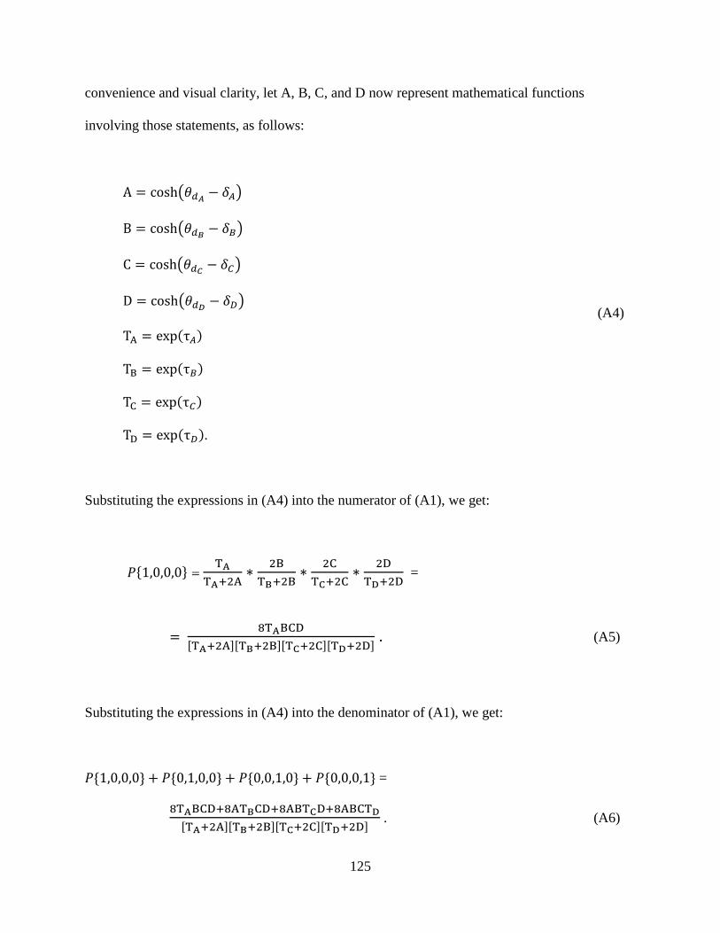
125
convenience and visual clarity, let A, B, C, and D now represent mathematical functions
involving those statements, as follows:
A = cosh�𝜃𝑑𝐴 − 𝛿𝐴�
B = cosh�𝜃𝑑𝐵 − 𝛿𝐵�
C = cosh�𝜃𝑑𝐶 − 𝛿𝐶�
D = cosh�𝜃𝑑𝐷 − 𝛿𝐷�
TA = exp(τ𝐴)
TB = exp(τ𝐵)
TC = exp(τ𝐶)
TD = exp(τ𝐷).
(A4)
Substituting the expressions in (A4) into the numerator of (A1), we get:
𝑃{1,0,0,0} = TA
TA+2A∗ 2BTB+2B
∗ 2CTC+2C
∗ 2DTD+2D
=
= 8TABCD[TA+2A][TB+2B][TC+2C][TD+2D] . (A5)
Substituting the expressions in (A4) into the denominator of (A1), we get:
𝑃{1,0,0,0} + 𝑃{0,1,0,0} + 𝑃{0,0,1,0} + 𝑃{0,0,0,1} =
8TABCD+8ATBCD+8ABTCD+8ABCTD[TA+2A][TB+2B][TC+2C][TD+2D] . (A6)
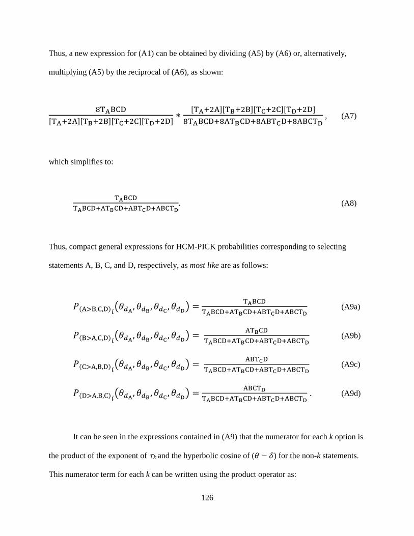
126
Thus, a new expression for (A1) can be obtained by dividing (A5) by (A6) or, alternatively,
multiplying (A5) by the reciprocal of (A6), as shown:
8TABCD[TA+2A][TB+2B][TC+2C][TD+2D] ∗
[TA+2A][TB+2B][TC+2C][TD+2D]8TABCD+8ATBCD+8ABTCD+8ABCTD
, (A7)
which simplifies to:
TABCDTABCD+ATBCD+ABTCD+ABCTD
. (A8)
Thus, compact general expressions for HCM-PICK probabilities corresponding to selecting
statements A, B, C, and D, respectively, as most like are as follows:
𝑃(A>B,C,D)𝑖�𝜃𝑑A ,𝜃𝑑B ,𝜃𝑑C ,𝜃𝑑D� = TABCD
TABCD+ATBCD+ABTCD+ABCTD (A9a)
𝑃(B>A,C,D)𝑖�𝜃𝑑A ,𝜃𝑑B ,𝜃𝑑C ,𝜃𝑑D� = ATBCD
TABCD+ATBCD+ABTCD+ABCTD (A9b)
𝑃(C>A,B,D)𝑖�𝜃𝑑A ,𝜃𝑑B ,𝜃𝑑C ,𝜃𝑑D� = ABTCD
TABCD+ATBCD+ABTCD+ABCTD (A9c)
𝑃(D>A,B,C)𝑖�𝜃𝑑A ,𝜃𝑑B ,𝜃𝑑C ,𝜃𝑑D� = ABCTD
TABCD+ATBCD+ABTCD+ABCTD . (A9d)
It can be seen in the expressions contained in (A9) that the numerator for each k option is
the product of the exponent of τk and the hyperbolic cosine of (𝜃 − 𝛿) for the non-k statements.
This numerator term for each k can be written using the product operator as:
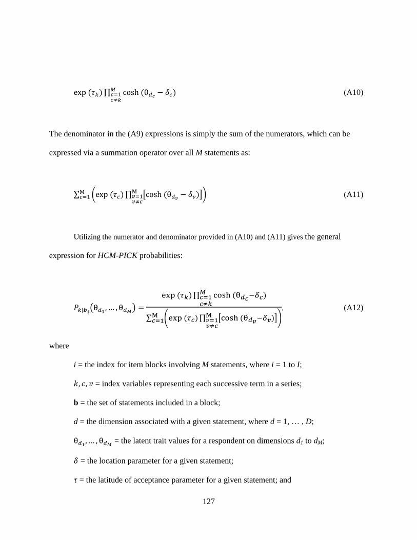
127
exp (𝜏𝑘)∏ cosh (θ𝑑𝑐 − 𝛿𝑐)𝑀𝑐=1𝑐≠𝑘
(A10)
The denominator in the (A9) expressions is simply the sum of the numerators, which can be
expressed via a summation operator over all M statements as:
∑ �exp (𝜏𝑐)∏ �cosh (θ𝑑𝑣 − 𝛿𝑣)�M𝑣=1𝑣≠𝑐
�M𝑐=1 (A11)
Utilizing the numerator and denominator provided in (A10) and (A11) gives the general
expression for HCM-PICK probabilities:
𝑃𝑘|𝒃𝑖�θ𝑑1 , … , θ𝑑𝑀� =
exp (𝜏𝑘)∏ cosh (θ𝑑𝑐−𝛿𝑐)𝑀𝑐=1𝑐≠𝑘
∑ �exp (𝜏𝑐)∏ �cosh (θ𝑑𝑣−𝛿𝑣)�M𝑣=1𝑣≠𝑐
�M𝑐=1
, (A12)
where
i = the index for item blocks involving M statements, where i = 1 to I;
𝑘, 𝑐, 𝑣 = index variables representing each successive term in a series;
b = the set of statements included in a block;
d = the dimension associated with a given statement, where d = 1, … , D;
θ𝑑1 , … , θ𝑑𝑀 = the latent trait values for a respondent on dimensions d1 to dM;
𝛿 = the location parameter for a given statement;
𝜏 = the latitude of acceptance parameter for a given statement; and

128
𝑃𝑘|𝑏𝑖�𝜃𝑑1 , … ,𝜃𝑑𝑀� = the probability of a respondent selecting statement k as most like in
the ith block of M statements.
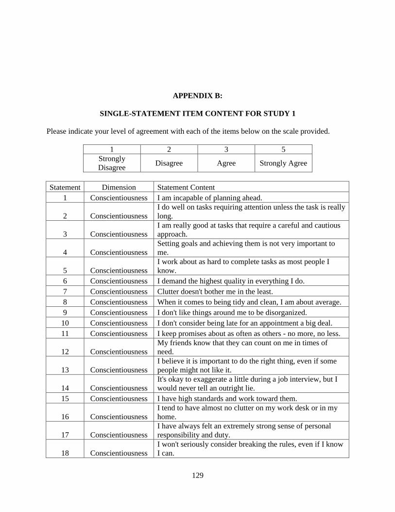
129
APPENDIX B:
SINGLE-STATEMENT ITEM CONTENT FOR STUDY 1
Please indicate your level of agreement with each of the items below on the scale provided.
1 2 3 5 Strongly Disagree Disagree Agree Strongly Agree
Statement Dimension Statement Content
1 Conscientiousness I am incapable of planning ahead.
2 Conscientiousness I do well on tasks requiring attention unless the task is really long.
3 Conscientiousness I am really good at tasks that require a careful and cautious approach.
4 Conscientiousness Setting goals and achieving them is not very important to me.
5 Conscientiousness I work about as hard to complete tasks as most people I know.
6 Conscientiousness I demand the highest quality in everything I do. 7 Conscientiousness Clutter doesn't bother me in the least. 8 Conscientiousness When it comes to being tidy and clean, I am about average. 9 Conscientiousness I don't like things around me to be disorganized. 10 Conscientiousness I don't consider being late for an appointment a big deal. 11 Conscientiousness I keep promises about as often as others - no more, no less.
12 Conscientiousness My friends know that they can count on me in times of need.
13 Conscientiousness I believe it is important to do the right thing, even if some people might not like it.
14 Conscientiousness It's okay to exaggerate a little during a job interview, but I would never tell an outright lie.
15 Conscientiousness I have high standards and work toward them.
16 Conscientiousness I tend to have almost no clutter on my work desk or in my home.
17 Conscientiousness I have always felt an extremely strong sense of personal responsibility and duty.
18 Conscientiousness I won't seriously consider breaking the rules, even if I know I can.
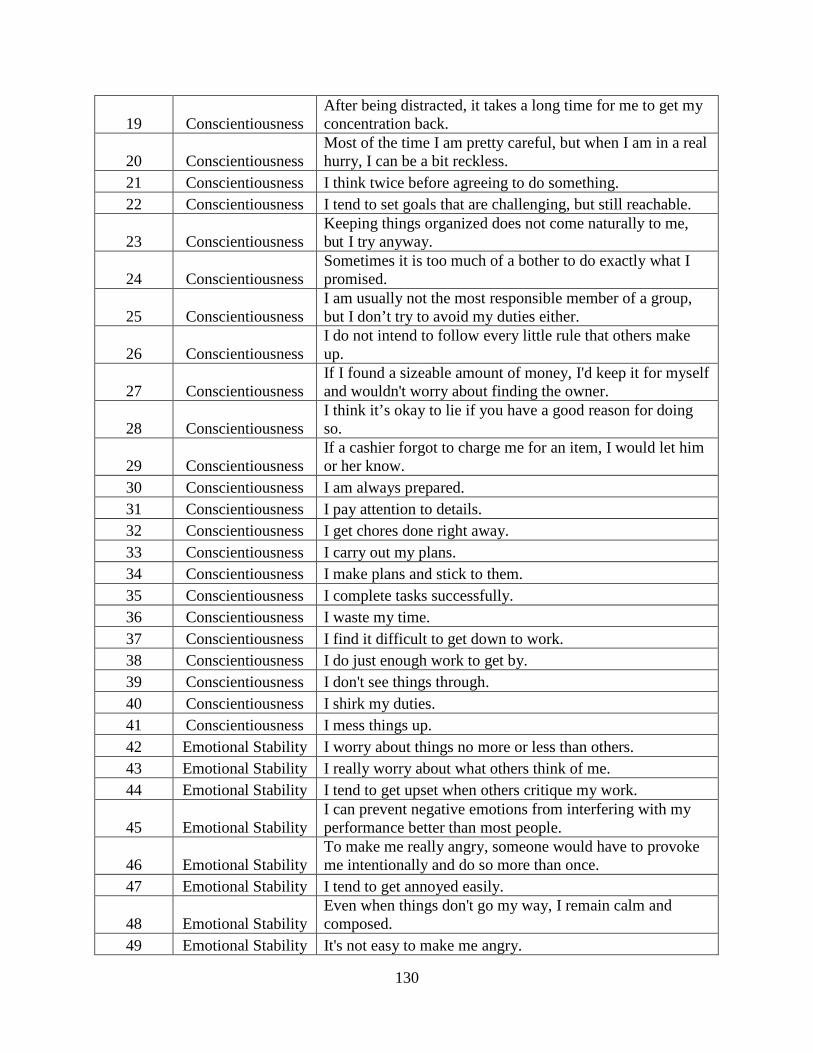
130
19 Conscientiousness After being distracted, it takes a long time for me to get my concentration back.
20 Conscientiousness Most of the time I am pretty careful, but when I am in a real hurry, I can be a bit reckless.
21 Conscientiousness I think twice before agreeing to do something. 22 Conscientiousness I tend to set goals that are challenging, but still reachable.
23 Conscientiousness Keeping things organized does not come naturally to me, but I try anyway.
24 Conscientiousness Sometimes it is too much of a bother to do exactly what I promised.
25 Conscientiousness I am usually not the most responsible member of a group, but I don’t try to avoid my duties either.
26 Conscientiousness I do not intend to follow every little rule that others make up.
27 Conscientiousness If I found a sizeable amount of money, I'd keep it for myself and wouldn't worry about finding the owner.
28 Conscientiousness I think it’s okay to lie if you have a good reason for doing so.
29 Conscientiousness If a cashier forgot to charge me for an item, I would let him or her know.
30 Conscientiousness I am always prepared. 31 Conscientiousness I pay attention to details. 32 Conscientiousness I get chores done right away. 33 Conscientiousness I carry out my plans. 34 Conscientiousness I make plans and stick to them. 35 Conscientiousness I complete tasks successfully. 36 Conscientiousness I waste my time. 37 Conscientiousness I find it difficult to get down to work. 38 Conscientiousness I do just enough work to get by. 39 Conscientiousness I don't see things through. 40 Conscientiousness I shirk my duties. 41 Conscientiousness I mess things up. 42 Emotional Stability I worry about things no more or less than others. 43 Emotional Stability I really worry about what others think of me. 44 Emotional Stability I tend to get upset when others critique my work.
45 Emotional Stability I can prevent negative emotions from interfering with my performance better than most people.
46 Emotional Stability To make me really angry, someone would have to provoke me intentionally and do so more than once.
47 Emotional Stability I tend to get annoyed easily.
48 Emotional Stability Even when things don't go my way, I remain calm and composed.
49 Emotional Stability It's not easy to make me angry.
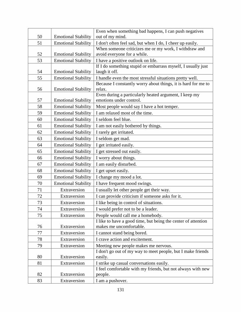
131
50 Emotional Stability Even when something bad happens, I can push negatives out of my mind.
51 Emotional Stability I don't often feel sad, but when I do, I cheer up easily.
52 Emotional Stability When someone criticizes me or my work, I withdraw and avoid everyone for a while.
53 Emotional Stability I have a positive outlook on life.
54 Emotional Stability If I do something stupid or embarrass myself, I usually just laugh it off.
55 Emotional Stability I handle even the most stressful situations pretty well.
56 Emotional Stability Because I constantly worry about things, it is hard for me to relax.
57 Emotional Stability Even during a particularly heated argument, I keep my emotions under control.
58 Emotional Stability Most people would say I have a hot temper. 59 Emotional Stability I am relaxed most of the time. 60 Emotional Stability I seldom feel blue. 61 Emotional Stability I am not easily bothered by things. 62 Emotional Stability I rarely get irritated. 63 Emotional Stability I seldom get mad. 64 Emotional Stability I get irritated easily. 65 Emotional Stability I get stressed out easily. 66 Emotional Stability I worry about things. 67 Emotional Stability I am easily disturbed. 68 Emotional Stability I get upset easily. 69 Emotional Stability I change my mood a lot. 70 Emotional Stability I have frequent mood swings. 71 Extraversion I usually let other people get their way. 72 Extraversion I can provide criticism if someone asks for it. 73 Extraversion I like being in control of situations. 74 Extraversion I would prefer not to be a leader. 75 Extraversion People would call me a homebody.
76 Extraversion I like to have a good time, but being the center of attention makes me uncomfortable.
77 Extraversion I cannot stand being bored. 78 Extraversion I crave action and excitement. 79 Extraversion Meeting new people makes me nervous.
80 Extraversion I don't go out of my way to meet people, but I make friends easily.
81 Extraversion I strike up casual conversations easily.
82 Extraversion I feel comfortable with my friends, but not always with new people.
83 Extraversion I am a pushover.
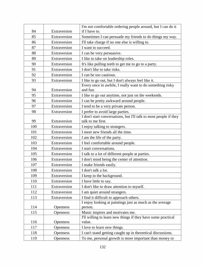
132
84 Extraversion I'm not comfortable ordering people around, but I can do it if I have to.
85 Extraversion Sometimes I can persuade my friends to do things my way. 86 Extraversion I'll take charge if no one else is willing to. 87 Extraversion I want to succeed. 88 Extraversion I can be very persuasive. 89 Extraversion I like to take on leadership roles. 90 Extraversion It's like pulling teeth to get me to go to a party. 91 Extraversion I don't like to take risks. 92 Extraversion I can be too cautious. 93 Extraversion I like to go out, but I don't always feel like it.
94 Extraversion Every once in awhile, I really want to do something risky and fun.
95 Extraversion I like to go out anytime, not just on the weekends. 96 Extraversion I can be pretty awkward around people. 97 Extraversion I tend to be a very private person. 98 Extraversion I prefer to avoid large parties.
99 Extraversion I don't start conversations, but I'll talk to most people if they talk to me first.
100 Extraversion I enjoy talking to strangers. 101 Extraversion I meet new friends all the time. 102 Extraversion I am the life of the party. 103 Extraversion I feel comfortable around people. 104 Extraversion I start conversations. 105 Extraversion I talk to a lot of different people at parties. 106 Extraversion I don't mind being the center of attention. 107 Extraversion I make friends easily. 108 Extraversion I don't talk a lot. 109 Extraversion I keep in the background. 110 Extraversion I have little to say. 111 Extraversion I don't like to draw attention to myself. 112 Extraversion I am quiet around strangers. 113 Extraversion I find it difficult to approach others.
114 Openness I enjoy looking at paintings just as much as the average person.
115 Openness Music inspires and motivates me.
116 Openness I'll willing to learn new things if they have some practical value.
117 Openness I love to learn new things. 118 Openness I can't stand getting caught up in theoretical discussions. 119 Openness To me, personal growth is more important than money or
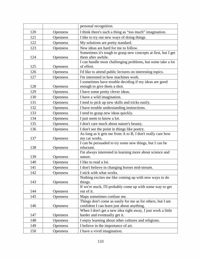
133
personal recognition. 120 Openness I think there's such a thing as “too much” imagination. 121 Openness I like to try out new ways of doing things. 122 Openness My solutions are pretty standard. 123 Openness New ideas are hard for me to follow.
124 Openness Sometimes it's tough to grasp new concepts at first, but I get them after awhile.
125 Openness I can handle most challenging problems, but some take a lot of effort.
126 Openness I'd like to attend public lectures on interesting topics. 127 Openness I'm interested in how machines work.
128 Openness I sometimes have trouble deciding if my ideas are good enough to give them a shot.
129 Openness I have some pretty clever ideas. 130 Openness I have a wild imagination. 131 Openness I tend to pick up new skills and tricks easily. 132 Openness I have trouble understanding instructions. 133 Openness I tend to grasp new ideas quickly. 134 Openness I just seem to know a lot. 135 Openness I don't care much about nature's beauty. 136 Openness I don't see the point in things like poetry.
137 Openness As long as it gets me from A to B, I don't really care how my car works.
138 Openness I can be persuaded to try some new things, but I can be reluctant.
139 Openness I'm always interested in learning more about science and nature.
140 Openness I like to read a lot. 141 Openness I don't believe in changing horses mid-stream. 142 Openness I stick with what works.
143 Openness Nothing excites me like coming up with new ways to do things.
144 Openness If we're stuck, I'll probably come up with some way to get out of it.
145 Openness Maps sometimes confuse me.
146 Openness Things don't come as easily for me as for others, but I am confident I can learn just about anything.
147 Openness When I don't get a new idea right away, I just work a little harder and eventually get it.
148 Openness I enjoy learning about other cultures and religions. 149 Openness I believe in the importance of art. 150 Openness I have a vivid imagination.
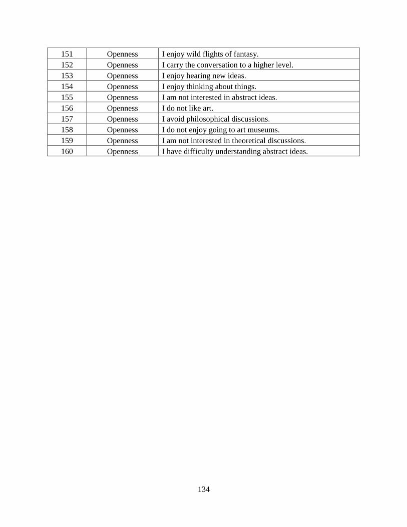
134
151 Openness I enjoy wild flights of fantasy. 152 Openness I carry the conversation to a higher level. 153 Openness I enjoy hearing new ideas. 154 Openness I enjoy thinking about things. 155 Openness I am not interested in abstract ideas. 156 Openness I do not like art. 157 Openness I avoid philosophical discussions. 158 Openness I do not enjoy going to art museums. 159 Openness I am not interested in theoretical discussions. 160 Openness I have difficulty understanding abstract ideas.
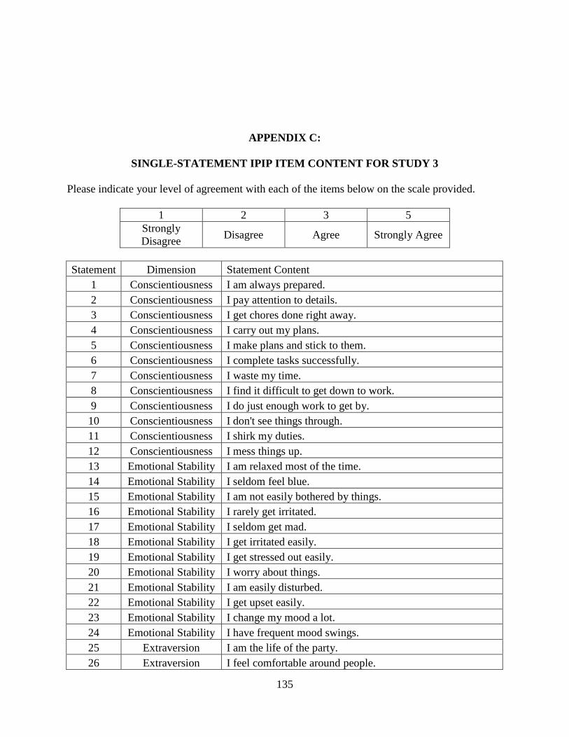
135
APPENDIX C:
SINGLE-STATEMENT IPIP ITEM CONTENT FOR STUDY 3
Please indicate your level of agreement with each of the items below on the scale provided.
1 2 3 5 Strongly Disagree Disagree Agree Strongly Agree
Statement Dimension Statement Content
1 Conscientiousness I am always prepared. 2 Conscientiousness I pay attention to details. 3 Conscientiousness I get chores done right away. 4 Conscientiousness I carry out my plans. 5 Conscientiousness I make plans and stick to them. 6 Conscientiousness I complete tasks successfully. 7 Conscientiousness I waste my time. 8 Conscientiousness I find it difficult to get down to work. 9 Conscientiousness I do just enough work to get by. 10 Conscientiousness I don't see things through. 11 Conscientiousness I shirk my duties. 12 Conscientiousness I mess things up. 13 Emotional Stability I am relaxed most of the time. 14 Emotional Stability I seldom feel blue. 15 Emotional Stability I am not easily bothered by things. 16 Emotional Stability I rarely get irritated. 17 Emotional Stability I seldom get mad. 18 Emotional Stability I get irritated easily. 19 Emotional Stability I get stressed out easily. 20 Emotional Stability I worry about things. 21 Emotional Stability I am easily disturbed. 22 Emotional Stability I get upset easily. 23 Emotional Stability I change my mood a lot. 24 Emotional Stability I have frequent mood swings. 25 Extraversion I am the life of the party. 26 Extraversion I feel comfortable around people.
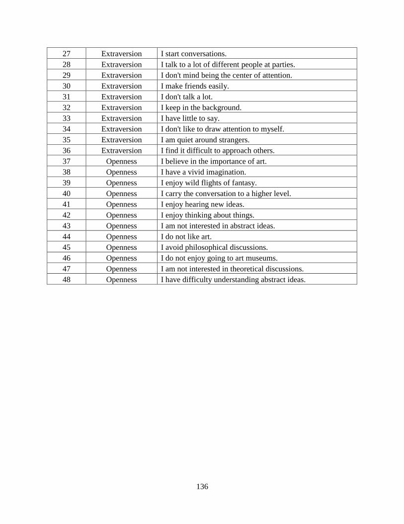
136
27 Extraversion I start conversations. 28 Extraversion I talk to a lot of different people at parties. 29 Extraversion I don't mind being the center of attention. 30 Extraversion I make friends easily. 31 Extraversion I don't talk a lot. 32 Extraversion I keep in the background. 33 Extraversion I have little to say. 34 Extraversion I don't like to draw attention to myself. 35 Extraversion I am quiet around strangers. 36 Extraversion I find it difficult to approach others. 37 Openness I believe in the importance of art. 38 Openness I have a vivid imagination. 39 Openness I enjoy wild flights of fantasy. 40 Openness I carry the conversation to a higher level. 41 Openness I enjoy hearing new ideas. 42 Openness I enjoy thinking about things. 43 Openness I am not interested in abstract ideas. 44 Openness I do not like art. 45 Openness I avoid philosophical discussions. 46 Openness I do not enjoy going to art museums. 47 Openness I am not interested in theoretical discussions. 48 Openness I have difficulty understanding abstract ideas.

137
APPENDIX D:
4-D MFC TETRAD MEASURE FOR STUDY 3
Block Dimension Statement Content 1 Conscientiousness I am incapable of planning ahead.
Emotional Stability I really worry about what others think of me.
Extraversion I usually let other people get their way.
Openness I can't stand getting caught up in theoretical discussions.
2 Conscientiousness Setting goals and achieving them is not very important to me.
Emotional Stability When someone criticizes me or my work, I withdraw and avoid everyone for a while.
Extraversion I would prefer not to be a leader.
Openness New ideas are hard for me to follow.
3 Conscientiousness Clutter doesn't bother me in the least.
Emotional Stability I tend to get upset when others critique my work.
Extraversion People would call me a homebody.
Openness I think there's such a thing as “too much” imagination.
4 Conscientiousness I don't consider being late for an appointment a big deal.
Emotional Stability I tend to get annoyed easily.
Extraversion Meeting new people makes me nervous.
Openness I'll willing to learn new things if they have some practical value.
5 Conscientiousness I do well on tasks requiring attention unless the task is really
long.
Emotional Stability I worry about things no more or less than others.
Extraversion I like to have a good time, but being the center of attention makes me uncomfortable.
Openness I can handle most challenging problems, but some take a lot of effort.
6 Conscientiousness I work about as hard to complete tasks as most people I know.
Emotional Stability Even when something bad happens, I can push negatives out of my mind.
Extraversion I can provide criticism if someone asks for it.
Openness I enjoy looking at paintings just as much as the average person.
7 Conscientiousness When it comes to being tidy and clean, I am about average.

138
Emotional Stability To make me really angry, someone would have to provoke me intentionally and do so more than once.
Extraversion I don't go out of my way to meet people, but I make friends easily.
Openness My solutions to problems are pretty standard.
8 Conscientiousness I keep promises about as often as others.
Emotional Stability I don't often feel sad, but when I do, I cheer up easily.
Extraversion I feel comfortable with my friends, but not always with new people.
Openness Sometimes it's tough to grasp new concepts at first, but I get them after awhile.
9 Conscientiousness I am really good at tasks that require a careful and cautious
approach.
Emotional Stability Even when things don't go my way, I remain calm and composed.
Extraversion I strike up casual conversations easily.
Openness Music inspires and motivates me.
10 Conscientiousness I don't like things around me to be disorganized.
Emotional Stability It's not easy to make me angry.
Extraversion I like being in control of situations.
Openness I love to learn new things.
11 Conscientiousness My friends know that they can count on me in times of need.
Emotional Stability I can prevent negative emotions from interfering with my performance better than most people.
Extraversion I cannot stand being bored.
Openness To me, personal growth is more important than money or personal recognition.
12 Conscientiousness I demand the highest quality in everything I do.
Emotional Stability I have a positive outlook on life.
Extraversion I crave action and excitement.
Openness I like to try out new ways of doing things.