X-641-67-13,,

A NEW LOOK AT THE BROWN-TWISS

INTERFEROMETER

FRANK C. JONES

REVISEDOCTOBER1967

GODDARDSPACEFLIGHTCENTERGREENBELT,MARYLAND

• TO8 1 4

o _g /(PAGES)

.__,,._" _-s-_/_7 '7#(NASA CR OR TMX OR AD NUMBgR) (C_EGO#Ry)

L

https://ntrs.nasa.gov/search.jsp?R=19680002357 2018-07-22T12:18:51+00:00Z

i

A NEW LOOK AT THE BRO.WN-TW!_SS INTERFEROMETER

by

Frank C. Jones

NASA Goddard Space Flight Center

Greenbelt, Maryland

ABSTRACT

A question that often arises when one is attempting to understand the prin-

ciples underlying the Brown-Twiss stellar interferometer is "How can there be

any kind of interference phenomena with light produced by incoherent sources ?"

Starting from the familiar interference pattern produced by two coherent sources

we may proceed in simple steps to a picture of two incoherent sources produc-

ing an interference pattern that jumps about at random. This randomly jumping

pattern leaves behind a "footprint," however, in the form of the intensity auto-

correlation function. We will see how the autocorrelation function for an ex-

tended, incoherent source may be constructed and that it is this function that is

measured by the Brown-Twiss stellar interferometer.

\

A NEW LOOK AT THE BROWN-TWISS INTERFEROMETER

by

Frank C. Jones

NASA Goddard Space Flight Center

Greenbelt, Maryland

I. Introduction

The physical principles underlying interference phenomena such as the pat-

tern produced by a diffraction grating or a double slit interferometer are under-

stood by practically everyone who has studied physical optics. On the other hand

ten or more years after the basic papers of Hanbury, Brown and Twiss 1, 2 de-

scribing the principles and operation of their post-detection stellar interferom-

eters a considerable area of confusion still exists in the minds of many physicists,

both students and professionals, concerning the fundamental concepts employed

in their operation. This condition persists in spite of the considerable number

of papers which have since been published 3 that investigate this phenomenon in

great detail.

There appear to be two main areas of confusion in this matter. The first

concerns the correlation of arrival times of two separate photons at two separate

detectors. This appears to be in contradiction with a basic principle of quantum

electrodynamics which is, as stated by Dirac, 4 "Each photon then interferes only

with itself. Interference between two different photons never occurs."

This question has been answered quite clearly by Purcell s and by Mandel 6

to the effect that while two photons can not interfere with each other they may be

correlated by virtue of their being bosons and their tendancyto clump together

in phase space.

It would be difficult to improve on the clarity of the treatment of the quantum

problem foundin references 5 and 6. A brief discussion of this matter is given

in Appendix I, therefore, only for background. In fact, this treatment leans heavily

on that of Mandel.6 The primary result of this discussion is that the operation of

the stellar interferometer can be understood entirely from the point of view of

classical electromagnetic theory, a point that has beenemphasized by Hanbury

Brown and Twiss. 2 In fact the validity of the semi-classical approach to a wide

variety of electromagnetic phenomenahas recently been demonstrated by Mandel

andWolf. 7

The second question is purely classical in nature and is essentially: "How

is it possible to have any kind of interference phenomena with light from inco-

herent sources ?" Although this question has been extensively diseussed, s to

those not familiar with the rather technical literature on the coherence proper-

ties of radiation from incoherent sources it remains somewhat of a puzzle. It

is to this question that the present paper is addressed.

In Section II we shall develop a treatment of the spatial dependence of inten-

sity correlations starting with the simple, first-order interference pattern pro-

duced by two coherent sources. From this simple concept we will proceed in

simple steps to (it is hoped) an understanding of the physical principles of the

post detection stellar interferometer of Hanbury Brown and Twiss.

H. The Spatial Dependence of Intensity Fluctuation Correlation

The essential element in the post-detection interferometer is a detector of

electromagnetic radiation whose response is proportional to the intensity, I, of

2

the radiation. This can be a radio receiver with a "square-law" detector circuit

or, in the optical region of the spectrum, a photo-electric cell. In Appendix I it

is shownthat, although the photo-electric cell responds to individual photons,

for the purpose of studying the statistical correlation betweenthe outputof two

separate detectors we may ignore this fact and assume that its output is directly

proportional to the classical intensity.

Actually no detector has a zero resolution time and rather than having an

output, 0 (t), directly proportional to the instantaneousintensity, I (t), the

appropriate quantity will be u (t) where

u (t) cc I (t) dt. (1)

-T

In this expression T represents the resolution time of the detector. If we

define the coherence time, A t, of the radiation to be the characteristic time

during which the intensity varies only slightly and if we choose T << At we have

u(t)oc T I (t). (2)

This assumption is actually quite reasonable for the radio-interferometer 1

but not in the optical case. 2 The complications involved in the case where T >__At

in no way change the basic principles that we shall consider but they do make

the treatment more difficult. For this reason we shall assume in what follows

that the output of any detector under discussion is directly proportional to the

instantaneous intensity of radiation falling upon it.

In the operation of the post-detection interferometer two detectors, A and

B, are separated by a distance, 8. Their outputs are passed through filters

which remove the steadycomponentand allow only the fluctuations to pass. In

other words the output of a filter is proportional to I (t) -_I_ where the brackets

< _ represent a time average. The outputs from the two filters are multiplied

together andtime averaged in a circuit called a correlator: the output of the

correlator, CAB' is therefore,

CABc0 <(I A(t)- _I A(t)_) (I,(t)- _I B(t)_

= <IAIB>- <I^> <I. >

Figure 1 is a schematic representation of this arrangement.

(3)

It is clear that we now wish to examine the relationship between the corre-

lation of intensity fluctuations in two separated detectors, on the one hand, and

the structure of the source of radiation, on the other.

We start with the simplest possible picture of two sources, 1 and 2, located

at r 1 and r 2 each radiating a monochromatic wave of frequency w and ampli-

tudes A1 and A 2. At first we shall consider their amplitudes to be constant.

However, each source will have a phase, ¢1 (t) and ¢2 (t), that will change with

time in a random way but with d¢/d t _ i/At << cv. The important point to note

is that although the two sources have no fixed relative phase, at any given time

a certain instantaneous phase difference, ¢1 (t) - ¢2 (t), does exist. Neglect of

this point causes much of the confusion concerning the possibility of interference

phenomena existing for incoherent sources.

At the origin of our coordinate system the amplitude from both sources is

given by

A =A 1exp i [r I +_t +¢1 (t - rl/c )]

+ A 2 cxp i [r 2 + -._t + ¢2 (t - r2/e ) ] _a_

In the above expression the amplitudes, A1 and A2, are the amplitudes at the

origin from source 1 and 2 respectively, and r I and r 2 are measured in wave-

lengths, c/_, for simplicity. The corresponding intensity will be given by

I (t) = A12 +A_ + 2A1A 2 cos (r 1-r 2 +¢l(t-rl/c ) - ¢2 (t - r2/c)). (5)

If we move to a point a distance, x, away from the origin keeping t fixed,

and assume that x << rl, r 2 (and for observations made on the earth of astro-

nomical objects this is extremely valid), the distances from the sources to the

new position are given by

#

r I* _ r I - r| • x', r2 _ r2 - r2 " x

where £` = r/r, a unit vector.

A

We have for the intensity at the point, x, (since we may safely take AI (x) =

i etc.)

I (x_ t) = A 2 + A 2 + 2A1A 2 cos (r 1 - r 2 - x • el2 + ¢12 (x, t)), (6)

where O 12 = 21 - £`2, and for small values is just the angular separation between

sources 1 and 2, ¢12 (x, t) is the new relative phase angle given by

¢12 (X, t) = ¢1 (t - rl/C + rl " x/c) -- ¢2 (t - r2/c + £'2 " X/C).

We may now ask to what extent equation (6) represents a well defined inter-

ference pattern. We note first of all that we do not know the overall phase of the

cosine function, since we do not know r 1 - r 2 (certainly not to within a wave-

length) and we do not know the phase factor ¢12" However, the behaviour of (6)

as a function of x is well defined provided the phaseangles do not changeappre-

ciably (for if they do, they changein a random way andwe are lost). To assure

this we must have 21 • x _ 22• x <<cat, since ¢ (t) is essentially constant for

times small compared to _ t. We can achieve this by requiring 21 "x = 22 x

= 0, but this would make x • e12 = 0 and we would have no dependence on x at

all. The best compromise, therefore, is to set 1 x. (21 + 22) = 0, or in other2

words to stay on a plane perpendicular to the average direction of the sources

(see Figxtre 2). In practice _ ,2 this is achieved by inserting a time delay in the

circuitry of the detector at x equal to -_ t = 1/2 (21 + E2) • x/c which has the

same effect on the arguments of ¢1 and ¢2"

Using either approach we may write the arguments of ¢1 and ¢2 as, t -

rl/c+ 21 • x/c- 1/2 (21 + 22) • x/c =t - rl/c + e]2 "x/2c, andt - r2/c -

e12 • x/2crespectively. We now require that e12- x << 2c5t. But we have re-

quired d_0/dt _ 1/At<<o_ and since _ = c in our units we have 2cAt >> 1..

Therefore e12 .x may vary through many times 2 77 without appreciably chang-

ing ¢1 or ¢2.

With these considerations we may write (6) as

I(x, t)= 11 + 12 + 2 ¢_1I 2 cos (e12 • x + ¢12(t)), (7)

where we have dropped the constant (and unknown) factor, r I - r 2, and have

written 11 and 12 for A_ and A_ respectively. We see that what we have is

just a standard coherent interference pattern, but one that will not stand still.

It jumps from place to place staying in one spot only for times less than At.

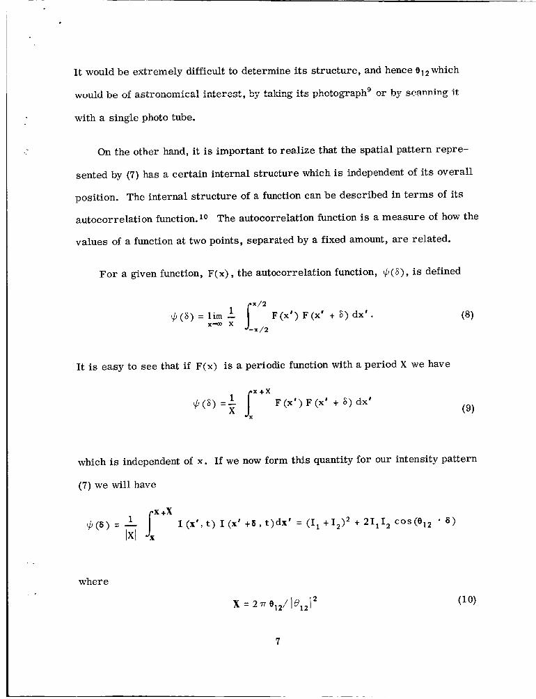
It would be extremely difficult to determine its structure, and hencee12which

___ _, 1__ --," --,-- ..... ,'_1 _,,-_.,,.,._+ 1-.,,_ +,-, I.,..t.n ,.,- 4.1-_ nh_fr_o"T-_h 9 n'r' h'_r ._r_DnJng" it..WULL].U L)_ UmL _::L_L.L UJ.IUIll.LS.,O.JL J.Zit,_JL _S,, PJy I,_.*_.L*Z_ _ l.,*_vvv_--_l.- ...... ,.,, ...... ,_ --

with a single photo tube.

On the other hand, it is important to realize that the spatial pattern repre-

sented by (7) has a certain internal structure which is independent of its overall

position. The internal structure of a function can be described in terms of its

autocorrelation function, z0 The autocorrelation function is a measure of how the

values of a function at two points, separated by a fixed amount, are related.

For a given function, F(x), the autocorrelation function, q_(6), is defined

x/2_b(S) = lim 1 F(x') F(x' + _) dx' o

x-,co X "_-x/2

(s)

It is easy to see that if F(x) is a periodic function with a period X we have

fx x +X1 F(x')F(x' + S) dx'

(9)

which is independent of x. If we now form this quantity for our intensity pattern

(7) we will have

fx x+X= _ I (x', t) I (x' +8, t)dx' = (I I +I2)2 + 2Ill 2 cos(el2 " 8)

¢(8) Ix]

where

:K = 2"rr el2/]Oz2J 2 (i0)

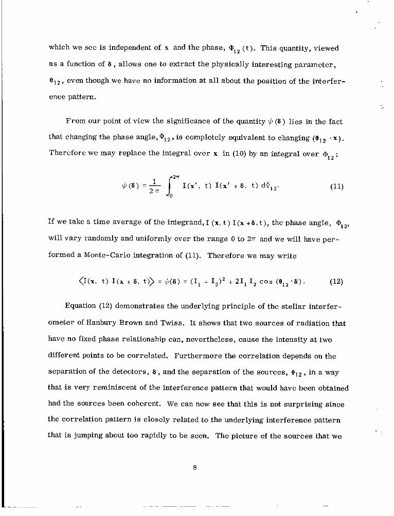
which we see is independent of x and the phase, ¢12 (t). This quantity, viewed

as a function of S, allows one to extract the physically interesting parameter,

el 2, even though we have no information at all about the position of the interfer-

ence pattern.

From our point of view the significance of the quantity _b(S) lies in the fact

that changing the phase angle, ¢12, is completely equivalent to changing (e12 .x).

Therefore we may replace the integral over x in (10) by an integral over ¢12 ;

f0 2_1 I(x' t) I(x' +S, t)d}12. (ii)¢ (s) : 2-7

If we take a time average of the integrand, I (x, t) I(x +_,t), the phase angle, ¢12,

will vary randomly and uniformly over the range 0 to 277 and we will have per-

formed a Monte-Carlo integration of (11). Therefore we may write

<I(x, t) I(x + S, t)> : _(S) -- (I 1 + I2)2 ÷ 2I 1 12 cos ({}12 "S). (12)

Equation (12) demonstrates the underlying principle of the stellar interfer-

ometer of Hanbury Brown and Twiss. It shows that two sources of radiation that

have no fixed phase relationship can, nevertheless, cause the intensity at two

different points to be correlated. Furthermore the correlation depends on the

separation of the detectors, S, and the separation of the sources, e12, in a way

that is very reminiscent of the interference pattern that would have been obtained

had the sources been coherent. We can now see that this is not surprising since

the correlation pattern is closely related to the underlying interference pattern

that is jumping about too rapidly to be seen. The picture of the sources that we

have considered so far is very simple andnot very realistic. We shall refine it

as we proceed until we have a picture that resembles a real astronomical object.

Nevertheless the basic principle will remain that expressed in equation (12).

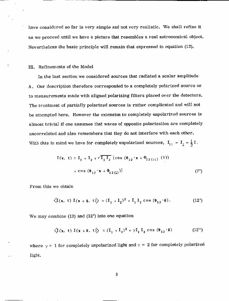
I_. Refinements of the Model

In the last section we considered sources that radiated a scalar amplitude

A. Our description therefore corresponded to a completely polarized source or

to measurements made with aligned polarizing filters placed over the detectors.

The treatment of partially polarized sources is rather complicated and will not

be attempted here. However the extension to completely unpolarized sources is

almost trivial if one assumes that waves of opposite polarization are completely

uncorrelated and also remembers that they do not interfere with each other.

this in mind we have for completely unpolarized sources, I,, = I 1 = 1 IWith o

I(x, t) = 11 + 12 + I1Y/_ 2 [cos (e12.x + q_12(,_) (t))

+ cos (e12.x + ¢12(1))] (7')

From this we obtain

<I(x, t) I(x + S, t)) : (I 1 + I2)2 + 11 12 cos ({}12 "S). (12')

We may combine (12) and (12') into one equation

_I(x, t) I(x +S, t)_ = (I 1 + I2)2 + VI 1 12 cos ({}12"S) (12")

where y = 1 for completely unpolarized light and y = 2 for completely polarized

light.

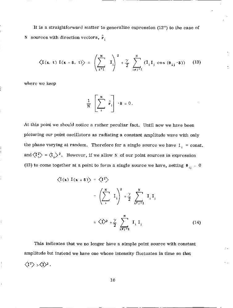
It is a straightforward matter to generalize expression (12") to the case of

N sources with direction vectors, r i

<I(x, t) l(x +8, t)> = I +-_i=1 iy_j =1

(IiI j cos (eij-8)) (13)

where we keep

At this point we should notice a rather peculiar fact. Until now we have been

picturing our point oscillators as radiating a constant amplitude wave with only

the phase varying at random. Therefore for a single source we have I i = const.

and <I_> = <Ii>2. However, if we allow N of our point sources in expression

(13) to come together at a point to form a single source we have, setting eij = 0

N

Y _ I.I.+_" I ;

i_j=1

N

<b 112+_ _ Ji_j =1

(14)

This indicates that we no longer have a simple point source with constant

amplitude but instead we have one whose intensity fluctuates in time so that

I0

If we realize that any macroscopic source of radiation (where macroscopic

means of dimension very large compared to the waveiength) is in fact made up

of many microscopic oscillators we see that our "point" sources should be con-

sidered as being made up of many small identical oscillators. To answer the

question of how many oscillators should contribute to one source we consider

equation (14) for N equal oscillators where I i = <I_/N. We have then

N

7 _, IIi_j=l

1 N(N - 1) _)=<I} _ + N2

<I>2 (1+_2 _N) (15)

If we choose N = co we have for any point oscillator the relation

(16)

It may be objected that this picture of a point source as made up of a very

large number of oscillators, all oscillating with a steady amplitude but con-

stantly changing phase is not very realistic. This is true. However, in Appen-

dix II it is shown that a far more realistic model of a radiation source also

yields equation (16). This is not too surprising; it is merely one more example

of the statistical law of large numbers. This law asserts that the probability

distributions of a quantity which is a sum of N random quantities approaches a

11

Gaussian as N becomesinfinite. In our case this means that the statistical

properties of the output from N oscillators become independentof the proper-

ties of the individual oscillators as N becomesvery large.

We now see that in deriving our expression for the autocorrelation of the

intensity, expression (12"), we shouldhave taken time averages of the individual

terms taking into accountthe fluctuations of 11 and 12 . Equation (12") becomes

<l(x, t) l(x +B, t)>: <(I, + 12)2> +_<I,12> cos (e12"8) (17)

and instead of (13) we have

<l(x, t)I(x+B, t) : I +7,i=l i_j=l

<IiIj> cos (Oil "B)

=I i_'j=I

(18)

Applying equation (16) and noting that <I i Ij> = <Ii> qj> because the intensity

fluctuations of two different sources are independent we have

N

<I(x, t)I(x +B, t)> = (1 +_),E <Ii>2i=l

N

i_j=11 +'>'cos (e i "8))2 i (19)

12

It is interesting to see that if we allow these sources to come together to

form one source we have

N N

i=l igj =I

N (>)

which is the same as (16) for a point source. This just shows that an infinity of

oscillators plus several other infinities of oscillators behaves like an infinity of

oscillators.

Equation (19) can be cast into a form that is quite suggestive; recalling that

Oil = r i - rj we have

N

i,j=l

i i ,j=l

exp (Jr i'8 - irj "8)

N L<Ii> exp (Jr i'8)

i=l

(21)

13

The generalization from N discrete sources to a continuous distribution of

sources is immediate. With the substitutions <Ii) _.I(r)d;_,

becomes

_ _I(r) exp (ir'8) d_ I<_(_ _(_+8_>= <_>_+_-

where I (r) is the source brightness per solid angle in the direction r.

S-_ f equation (21)1

(22)

Returning to equation (3)we may identify I A with I(x) and I s with I(x+8)°

It is easy to verify that <I(x)> = <I(x + 8)> = <I> and we may therefore sub-

stitute equation (22) into (3) to obtain for the output of the correlator

CA B _c{<_(x) ,(. +8)>- <,(x)> <_(x+8)>}

_ (_-) exp (Jr.8) d_ (23)

It is of interest to note that the quantity 9(8) = f F(r) exp (it "8)d;) is the

quantity determined with the Michelson interferometer. By determining this

quantity as a function of 8 the complete brightness distribution over the face of

a star F(r) may be determined using the inverse Fourier transform

F(r) = (277) -2 _F(8) exp (- 1r'8). (24)

With the post-detection interferometer we may determine only IF(S) 12 and we

have no information about the phase of F(8). We are, therefore, not able to

uniquely reconstruct F(r) without the use of additional assumptions.

14

The aboveresult has beenobtainedunder the condition that d¢/dt be small

compared to the frequency w. This is equivalent to assuming that the source is

quasi-monochromatic, since anychangein ¢ introduces additional frequencies to

the wave and the condition de/dr <<o_ is the same as _o_ << o_ or in other words we

are dealing with a narrow band of frequencies. We will now examine what hap-

pens if we relax this condition.

We see immediately that equation (7) is no longer valid since we may not

consider the phase difference ¢12 to be independent of x. Because of this, equa-

tion (12) should be replaced by

.................... <I(x, t)I(x+ S,t)> = (I,+I2)2 + 21, 12C(0,2" _) (25)

where

C(012" ') -- 2 <COS (012 " X ÷¢12 (i, t))COS (812 " X+ 812 " 3 ÷ ¢12 (X ÷ _, t))_ (26)

If we write ¢12 (x+ 8, t) = ¢12 (x, t) +_¢12 (x+ _, t)we may expand the cosine

functions to obtain

C(012- _) = <COS (812 " _){COS 2 (012" X) [COS2 ¢12 COS _(_12

-- COS(Pl 2 sJ.FI(1)I2 sin_(1)12 ] H- sJ.i-i2 (812 • x) [sin 2 ¢12 cos A¢12

+ sin ¢12 cos ¢12 sinA¢12 ] - cos (012 • x)sin (812 • i)[cos 2 ¢12 sinA¢12

15

- sin2¢i2 sinA¢i2 + 2 sin¢i2 cos¢i2 cosA¢i2]}

- sin (012 " _) {COS 2 (012" X)[COS 2 ([:)12 sin _012

+cos012 sinq512 cosAO12]+sin 2 (012" x)[sin 2 qbl2 sinAq)12

- sinO12 cos¢12 cosAO12 ] +cos (012" x)sin (Or2" x)[cos 2 ¢t2 c°s/_¢t2

- sin2 ¢12 cos/X@12 - 2 sin O12 cos O12 sinAqb i2]}> (27)

where the arguments of O12 and A(D12 are understood. We shall now assume that

0i2 performs a random walk such that the distribution of /xO12 does not depend

on Oi2. The primary justification for such an assumption is that any natural model

of a light source would have this property.

Ifwe recall that uniform distributionof dpi2implies

1

and

(sin 012 COS ¢_12_ = 0

16

q

equation (27) becomes

: Re(eXp (i012 • 8) (exp (iA¢12/)) (28)

where Re means the real part and (exp (iA¢12)) can depend only on 012. 8 (not

on x) since we have assumed throughout the discussion that the statistical prop-

erties of the source do not depend on time and the arguments of ¢12 are just re-

tarded time.

The development from this point on proceeds exactly as before with the

simple substitution of our function C(812 • 8)for cos (012 • 8). Recalling that

A¢12 = z]¢ 2 -i_bl, we see that equation (21) becomes

(z(x) z(x + s))

N

i)2 Z(ii)i,j=l

(29)

17

/

proceeding,Before we should pause and consider the function qexp _.

If we form the autocorrelation function of the amplitude A i (t) we have

-- exp (ion-) <exp(i_(T))> -- exp (ion-)¢' (9-) (30)

The Fourier transform of _(T )is

_(w') : _(-r)exp(iw'T)dT -- _' (w'+co)0o

(31)

where _' (w')is the transform ore' (_-). The function_(J ) is called the

normalized power spectrum lo of the amplitude A i ( t ). It has this name because

it represents the relative amount of power radiated in the frequency interval oJ'

and o_' + dw'. lo If we therefore write

and substitute this expression in (29) we have

<l(x) l(x+ 8)) - <I> 2

____74_ _<Ii>

i=l

exp (i_ i • S-ion' "ri)_i' (a)')dw'

2

(32)

18

If we now abandonour practice of writing lengths in units of the wave length we

have B-_B/_ = 8_/c. We also have _-i = _i " _/'c and therefore we may write

(I(x) I(x+ 8)) - <I)2

N_<I,> exp [i_- i • B(o_-o/)/c] _' (oa')dca'Co

i = I

(33)

If we now assume that all of our sources have the same spectral distribution,

i.e. _bi (o_') (o_') for all i we may go to the limit of a continuously distrib-

uted source and write as the equivalent of equation (23)

CAB f_ F(_)exp[i_" $(o_-o/)/c]_' (w')dw'd.Q--O0

) exp [it" _'/c] _(o_') dold_

co

(34)

L

This result is valid for any spectral distribution assuming that the detector itself

is not frequency dependent in its characteristics. In any real situation _b(_ )

should be multiplied by the frequency response function of the detector since any

real detector is equivalent to one of our ideal detectors with a frequency filter

placed in front of it.

19

We cansee from (34) that if ¢(_ ) is sharply peakedabout a particular

frequency (quasi-monochromatic) we obtain our previous result equation (23).

It is fairly easy to see that the finite bandwidth of the input radiation causes a

loss of information in the sensethat the functionF(B_/c) gets "smeared out" over

the frequency distribution. For example, if the characteristic size of the source

is ®, F will have structure over values of _ of order c/_ or larger. If the spread

in frequency _ is such that A(c/_) -- (c/o_@)_/_ _ c/o_@or _/_, _ 1 the struc-

ture will be lost and eventhe overall size of the source cannotbe determined

with any great accuracy.

We seetherefore that eventhough our initial requirement d¢/dt <<oJ is not

strictly required it certainly indicates the best operating conditions and if it is

violated such that d¢/dt % co it is very difficult to obtain any information about

the source.

IV. Conclusions

We have seen that starting with the simple notion of an interference pattern

that jumps randomly around we may proceed through a series of simple steps to

the spatial correlation pattern of light from an extended source. This correla-

tion pattern exists because what we call incoherent sources are not really totally

incoherent. There exist short periods of time during which some phase relations

exist between the various parts of the source. During this same short period of

time therefore an interference pattern exists at the point of observation. Since

these phase relations between the various parts of the source do not persist this

interference pattern is constantly shifting and changing. However, during this

change certain internal structures of the interference pattern are constant due

2O

to the overall structure of the source. Thecorrelation pattern that we observe

with the Hanbury Brown and Twiss type o__L_,,_L_........,,_1 _=1.....u,_^_ IS" j_"°+ a ....._._

ure of this constant, internal structure.

V. A C KNOWLE DGME NT

The author wishes to thank Drs. T. G. Northrop and R. J. Drachman and Mr.

T. Kelsall for stimulating discussions concerning this paper.

21

APPEND_ I

THE CONNECTION BETWEEN QUANTUM

AND CLASSICAL DESCRIPTION

The primary method of detection of a photon in the optical range is through

the use of a detector that employs the photo-electric effect in its operation (e.g.,

a photo-electric tube). In fact we may define the detection of a photon in a light

beam as the ejection of an electron from the photo-cathode of some suitable de-

tector. In this context the concepts of photon and classical electromagnetic field

are related through a single consideration, namely, that for a photo-cathode il-

luminated by a light beam the instantaneous probability per unit time of emission

of a photo electron (detection of a photon) is proportional to the instantaneous

intensity of the electro-magnetic wave falling on the photo-cathode;

dP(1) = aI(t) dt (AI-1)

where dP(1) is the probability for one and only one photon to be detected in a time

d t and a is the proportionality coefficient. The probability for two photons to be

detected is of second order in dt and is considered negligible. From probability

theory we know that for a finite interval of time between t 1 and t 2 the proba-

bility for the detection of n photons is given by the Poisson distribution

[u(t 1, t2)]n exp [-u(t 1, t2)]Pu (n) = n ! (AI- 2)

22

where

t 2

u(tl' t2)- f aI(t) dt.1

Unfortunately, unless the intensity I(t) is a constant, the distribution Pu (n)

is not observable, for if one took statistics on successive intervals (t 1 , t 2 ),

(t2, t3) - - - (tn, t+l) one would find that in general the value of u (t n, t+ 1)

would vary from interval to interval. Expression (SI-2) would describe the dis-

tribution only for the collection of intervals that had a common value, say a 1,

for the variable u (see figure 3).

If the variable u varies from interval to interval such that the probability

of any interval having a particular value of u is given by P(u), the probability

of detecting n photons in any interval picked at random will be given by the

Poisson distribution averaged over all possible values of u ie.

fo m u n exp (-u) duP(n) = P(u) n! (AI-3)

It would be well at this point to ask what possible meaning can we give to

the instantaneous intensity I(t) or its integral over an interval u(t n, tn÷ 1)

since there seems to be no operational way to determine their values. The

number of photons detected in any given interval has no unique relationship to

the value of u for that interval. The answer must be that I and u are calcu-

lational devices used to determine the statistical properties of photo-electrons

from a photo-cathode. If one calculates the probability per unit time for ejec-

tion of a photo-electron due to a source of electromagnetic radiation some

23

distance away anddoes so strictly from the theory of quantumelectrodynamics

one finds that this probability is proportional to the absolutevalue squared of a

vector quantity A. Furthermore, it turns out that if the source is made up of a

large number of elementary quantum systems and is some distance away the

quantity A may be calculated to a very good degree of approximation by using

Maxwell's equations and considering A to be the classical vector potential and

hence ]AI 2 to be the classical intensity I(t).

We see, therefore, that although the quantities I(u) and u(t n, tn+ 1) are,

strictly speaking, not observables (although we shall see that their average

values may be operationally defined) nevertheless they are conceptually and

calculationally useful quantities.

If we now consider a large number of non-overlapping intervals of length T

we may inquire about the mean value and rms fluctuation of the number n of

detected photons in each interval. Employing the definition of a mean value

co

n=0

and making use of the relation

n! u n(n - p)! n!

n:O

f(n) l_(n) (AI-4)

exp (- u) = u p (AI-5)

24

we obtain

co co

nun<n> : p(u) _ oxp (-u) du

f0co

= P(u) u du : <u> . (AI-6)

This may be taken to be the operational definition of (u_, the average value of u.

The mean square fluctuation of n about its mean value will be given by

: <us> ÷ (u>_ <_>_

: <_> ÷ <¢u- <u> )_>

: <.> + <au2>. (AI-7)

The first term on the right hand side of (AI-7) is just what would be given

if light were a stream of classical particles, for then the statistics of the pho-

tons would be just Poissonian. The second term _/_u2_ which is a measure of

the fluctuations of the wave field due to interference phenomena of one sort or

another shows that the deviation of photon statistics from Poissonian due to their

boson nature can be determined solely from an investigation of the associated

classical electromagnetic field. In fact it can be shown n that the very existence

of the classical electromagnetic field is intimately connected with the boson

character of the photon.

25

We nowturn to the situation where two different detectors A and B are

situated at different points of space. For fixed values of uA and uB the emis-

sion of electrons from the two cathodesis completely independent so we have

(UA)nA (UB)"Bexp [- u A u B]_UAUB (nA' nB) = nA ! riB!

and

-- _UA (n A) _UB (n B) (AI-8)

_D(n A, n B) _- _f _(UA' u B) ]DUA' u B (hA' n B) du A du B • (AI-9)

Expression (AI-8) indicates the complete independence of the distributions

of n A and n B for given values of uA and u B . However, if u A and u B are not

distributed independently ie. P(UA,Us) 4 P (UA)P(UB) then P(n A, n B) _ P(nA) _(nB) in

general and nA and n B are not distributed independently. In other words a cor-

relation between uA and u B imposes a correlation between n A and n B .

In the operation of the stellar interferometer of Hanbury Brown and Twiss

the fluctuations in the "output" of two different detectors are multiplied together

in a circuit called a correlator and this product is averaged over time. The

"output" of a photoelectric detector will be a current or voltage that is propor-

tional to the number of photo-electrons ejected from its cathode during some

interval of time T which is essentially the resolution time of the detector.

The averaged output of the correlator will, therefore, be proportional to

<(n A - <hA>) (n B - <riB>)> = <nA nB> -- <hA> InB>

-- <u AuB> - (UA> <UB> (AI-10)

26

and we see that this output is directly expressible in terms of the fluctuations

of the classical electromagnetic intensity. If the fluctuations of u^ and u B are

independent then _u a u B) = _u^ _uB_ and there is no averaged output from the

correlator.

27

APPENDIX II

A DETAILED SOURCE MODEL

We now consider a model of a radiation source that is considerably more

realistic than the one employed in Section ]II. Instead of constructing the source

out of a large number of oscillators running with a constant amplitude and phases

that change randomly over a period of time At we shall construct our source

from a collection of oscillators that turn on at random times with random start-

ing phases and then after a time At turn off again.

This model is suggested, of course, by the picture of a hot gas whose atoms

are constantly being excited through collisions and then radiating their extra

energy away during a short time At.

The method we shall use was employed by Rice 12 in his calculations of the

"shot effect," however, for a different treatment of the same problem the reader

is referred to a paper by Janossy. 13

Consider a collection of oscillators situated at a point S. If the i th oscil-

lator at S turns on at t = 0 it will produce a field at R given by

Ai(t) = ei exp(i ¢i) F(t - ISRI/c) (An-l)

where ¢i is an overall phase angle and $i is a unit polarization vector perpen-

dicular to the line joining S and R. F(t) describes the characteristic output of

an oscillator and has the properties F(t) = 0 for t < 0 and F(t) _ 0 for T >> At

28

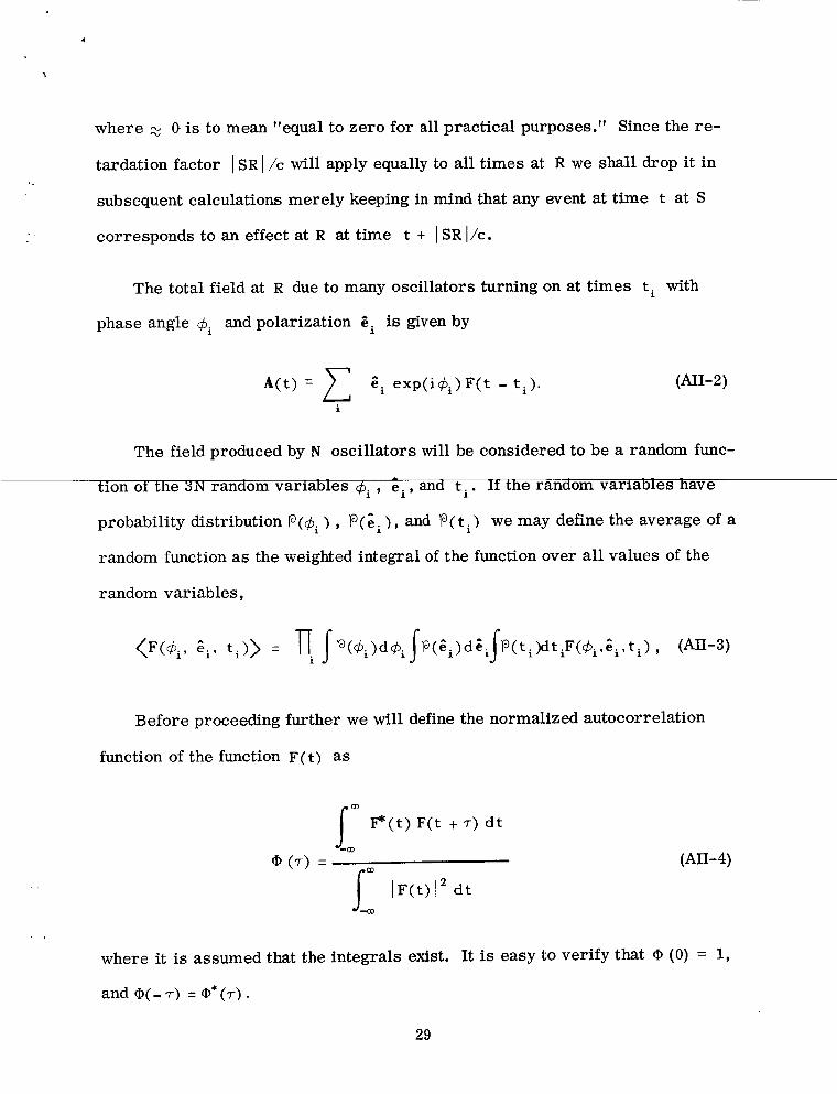
where _ 0 is to mean "equal to zero for all practical purposes." Since the re-

tardation factor ISRI/¢ will apply equally to all times at R we shall drop it in

subsequentcalculations merely keeping in mind that any event at time t at S

corresponds to an effect at R at time t + ISRI/c.

The total field at R due to many oscillators turning on at times t i with

phase angle ¢i and polarization _i is givenby

A(t) = _ ei exp(iq_i) F(t - ti). (AII-2)i

The field produced by N oscillators will be considered to be a random func-

tion oi the 3N random variables _b_, e i , and t_. If the random variables have

probability distribution P(_b i ), _(e i ), and P(t i) we may define the average of a

random function as the weighted integral of the function over all values of the

random variables,

<F(¢i' ei' ti)> = T_i fP(¢i)d¢ifP(ei)deifP(ti)dtiF(¢i'ei'ti )' (AII-3)

Before proceeding further we will define the normalized autocorrelation

function of the function F(t) as

f_ff F*(t) F(t + 7) dt

¢ (_) = (AII-4)

00 If(t) 12 dt00

where it is assumed that the integrals exist. It is easy to verify that ¢ (0) = 1,

and O(- 7) = _* (7).

29

Since F(t) is essentially zero everyone except for 0 < t < At we see that

¢(-i-) is essentially zero everywhere except for -At < "i- < At.

We now return to our amplitude function, expression (AII-2). For a process

that is stationary in time the sum should be over a infinite number of oscillators

over all times. Since it would be difficult to calculate averages with this quan-

tity directly we shall calculate with the subsidiary quantity AT(t ) which is the

amplitude produced by all of those oscillators with turn on times t. such that1

-T/2 < t i < T/2. At the end of the calculation we shall always take the limit

W-. 00.

We shall assume that the ti are independently and uniformly distributed

with a probability per unit time 77 where 77T is the average number turning on

in a time T. The phase angles ¢_ are independently and uniformly distributed

between 0 and 2 _. We shall leave consideration of the distribution of _. until1

later.

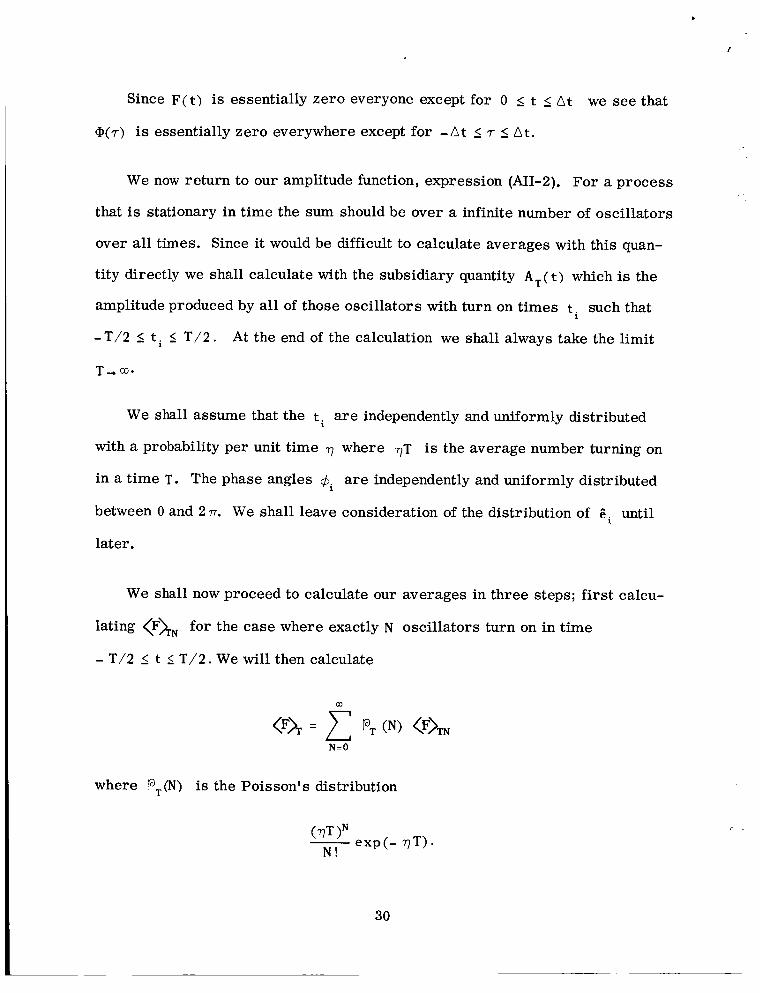
We shall now proceed to calculate our averages in three steps; first calcu-

lating _F_N for the case where exactly N oscillators turn on in time

- T/2 _<t < T/2. We will then calculate

co

N_-0

[aT (N) iF>TN

where PT(N) is the Poisson's distribution

(_TT) N

N_-- exp(- 77T).

3O

Finally we have

<F>: !iraT-.m

With these remarks in mind we consider first of all the intensity

I(t) =A*(t) A(t)

lj

(ei " ej) exp(iqSj - i¢i)F* (t - ti) F(t - tj) (AII-5)

.27T d¢i fP(%i) dei<I (t)>NT -- 2rTi=l -T/2

X (i _,j=l (ei'ej)exp(iqSJ -i(/)i)F*(t-ti)F(t-tj))

We can see immediately that only those terms in the sum where i = j

(AII-6)

give a

non-zero contribution after the phase angle averaging so we have (recalling

_. • _. =i)I 1

T/2

N£<I (t>NT =TT/2

dt i IF(t - t i) 12 (AII-7)

Since the time interval T can be as large as we wish, as long as t is not

too close to - T/2 or T/2 we may replace the integral over t F 12 by the infinite

integral to obtain(D

<i(t)>NT _ NT _ IF(t)[2 dt (AII-S)

31

<I(t)>T = Z <I(t)>NT PT(N)

N=O

co 0o

: -OT f_ IF(t)' 2 dt : -O f [F(t) 12dtW CO --03

The passage to the limit T -, m is now trivial and we have

(AII-9)

(3O

<I(t)> = "of IF(t) 12dt--CO

(AII-10)

The average intensity is thus seen to be just the intensity produced by a

single oscillator multiplied by the average number of oscillators turned on per

unit time; a rather intuitive result. We note that the result is independent of

the state of polarization, i.e., independent of P(_i )"

We turn now to the autocorrelation function of the intensity <¢(r)> defined

as ¢(r) : <I(t) I (t + _-)>.

We have

2rr P(ei) dei T/2 T

(ei " ej)(ek " el) expi(qSj - qbi +qS_-qSk)

j,k,l=l

x F*(t-ti)F(t-tj)F*(t +r-tk)F(t +r-tl) t"(AII-II)

32

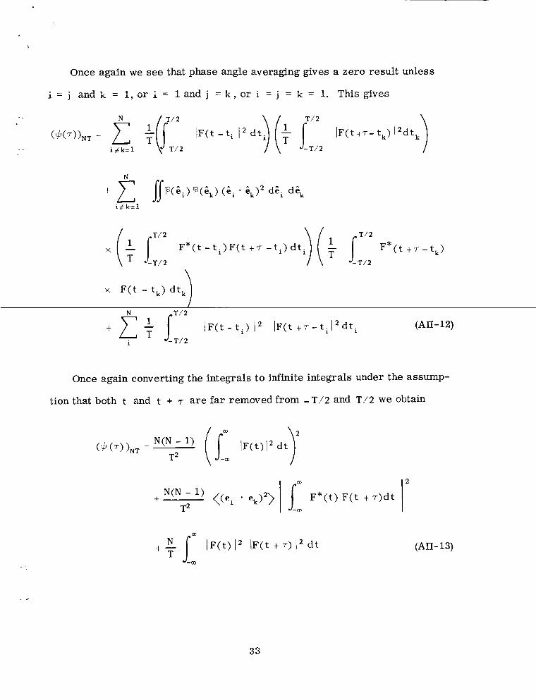
Once again we see that phase angle averaging gives a zero result unless

-- IF(t-t i 12 dt ]F(t+_-tk) 12dtk

i_k=l _-T/2 T/2

N

_f p(_i)_(_k)(_i " _k)2 d_i d_k

i_k=l

(1 f T/2 )(1x F*(t -ti)F(t +_ -ti) dt _-

-T/2

x F(t - tk) dtk)

fT/2

1+ -_- IF(t-t i) 12 [F(t +T-ti[2dti

i -T/2

T/2

F*(t +T-tk)-T/2

(AII-12)

Once again converting the integrals to infinite integrals under the assump-

tion that both t and t + _ are far removed from-T/2 and T/2 we obtain

(_(_-))NT - N(N - 1) ]F(t)] 2 dtT 2 co

N(N - 1)+ <(ei .%)2)T 2

F*(t) F(t + _-)dt

co

N f_ IF(t) L2÷¥co

IF(t + _)12 dt (AII-13)

33

where

2)

= /f P (ei) P(ek)(ei

o

%k )2 de i de n

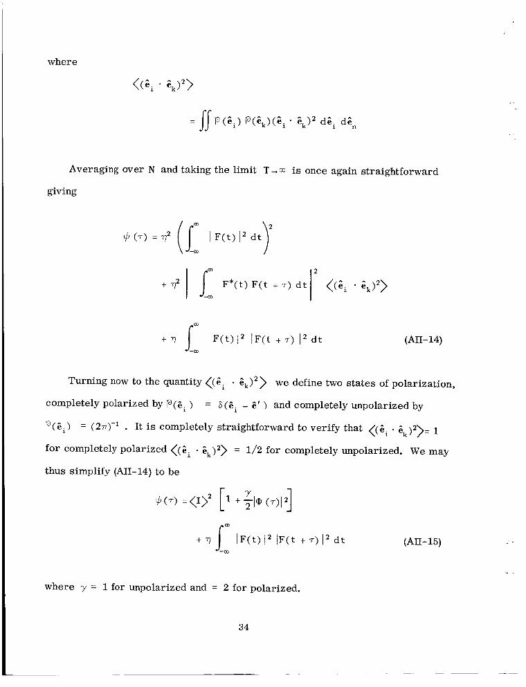
Averaging over N and taking the limit T-_ co is once again straightforward

giving

co

+ _2

IF(t) 12 dt) 2

co

I *(t) F(t + T) dtco

03

+ 7? i IF(t) 12 IF<t + _-) 12 dtco

(AII-14)

Turning now to the quantity ((_i " _k)2> we define two states of polarization,

completely polarized by P(gi ) = _(_i - _' ? and completely unpolarized by

P(_i ) = (27r) -I It is completely straightforward to verify that <(ei " _k)2> = 1

for completely polarized <(_i " _k)2> = 1/2 for completely unpolarized. We may

thus simplify (AII-14) to be

/. co

+ 77 / If(t) 12 IF(t + T) I2 dt (AII-15)J_

where y = I for unpolarized and = 2 for polarized.

34

..

In the limit of a very large 77 (this is equivalent to a large number of oscil-

lators being on at any given time) we may negiect the term linear in ?7 compared

to <1_2 which is quadratic in 77 giving

qJ(_) = <I_ [1 + 2 Igp (_)121 (AII-16)

a familiar result. .4

For z = 0 _(_-) = 1 and we have

(AII-17)

our desired result.

35

REFERENCES

I. R. HanburyBrown, and R. Q. Twiss, Phil. Mag. 45, 663 (1954).

2. R. Hanbury Brown, and R. Q. Twiss, Proc. Roy. Soc. (London) 242____A,300

(1957);243A, 291 (1957); 248A, 199 (1958); 248A, 222 (1958).

3. For a complete list of references see "Resource Letter OSL-I,"

P. Carruthers, Am. J. Phys. 31, 321 (1963).

4. P.A.M. Dirac, Quantum Mechanics (Oxford University Press, London,

1958), 3rd edition, p. 9.

5. E. M. Purcell, Nature, 178, 1449 (1956).

6. L. Mandel, Proc. Phys. Soc. (London) A72, 1037 (1958); A74, 233 (1959).

7. L. Mandel and E. Wolf, Phys. Rev. 149, 1033 (1966).

8. For a thorough review of this subject and extensive references see

L. Mandel and E. Wolf, Rev. Mod. Phys. 37, 231 (1965).

o This has, in fact, been done for the interference fringes produced by the

light from two lasers; see G. Magyar and L. Mandel, Nature 198, 255

(1963); Quantum Electronics (Proceedings of the Third International

Congress), edited by N. Bloembergen and P. Grivit (Dunod et Cie, Paris;

Columbia University Press, New York, 1964), p. 1247.

10. A good introduction to the autocorrelation function can be found in Y. W. Lee,

Statistical Theory of Communication (John Wiley and Sons, Inc., New York,

1960).

36

!!. E. M. Henley, and W. Thirring, Elementary Quantum Field Theory,

(McGraw-Hill Book Co., Inc., New York, 1962) p. 52.

12. S. O. Rice, Bell System Tech. J. 23, 282 (1944); 2__4,46 (1945).

-°

13. J. Janossy, Ii Nuovo Cimento, 6, Iii (1957).

14. J. L. Lawson, and G. E. Uhlenbeck, Threshold Signals (McGraw-Hill Book

Co., Inc., New York, 1950), p. 61.

37

FIGURE CAPTIONS

Fig. 1

Fig. 2

Fig. 3

Schematic of Post Detection Interferometer.

Instantaneous Interference Pattern Produced by Two Sources.

ti +1/.

of Time Intervals Having Different Values of u = _,/.Sequence

I

dr.

38

LIGHT, INTENSITY IA(t )

DETECTORA

I OUTPUT(_IA(t)

FILTER

LIGHT, INTENSITY IB(t )

DETECTOR

B

OUTPUT

ocIB(t)

GI

FILTER I

IA (t)-_IA(t)} IB (t)-- _IB(t)}

CORRELATOR

Fig. 1 Schematic of Post Detection Interferometer.

I"2

PLANE PERPENDICULAR TO

I/2 (,_+$2)

Fig. 2 Instantaneous Interference Pattern Produced by Two Sources.

_w

• %

Io=n

I_=n

IOD:n

I_0=n

z c50 I--

0

0 N

Lid -

-Io._1 1.1_.j 0

_mLLI

.d .-I

U.I ZI-- WZ

t_

--J LI_

D

z 0

Z tlA

_ a

t-- Z

0

_- rn

n,"

£10=n

Z1o=n

IIo =n

4J

v

+

II

0

:>

b9

I>f_q)

I,--I

q)

0

q2

or3

co