a new mesh-free vortex method p-hd thesis

A NEW MESH-FREE VORTEX METHOD

Name: Shankar Subramaniam

Department: Department of Mechanical Engineering

Major Professor: Leonard van Dommelen

Degree: Doctor of Philosophy

Term Degree Awarded: Fall, 1996

A new method is proposed for simulating diffusion in vortex methods for incompress-

ible flows. The method resolves length scales up to the spacing of the vortices. The

grid-free nature of vortex methods is fully retained and the distribution of the vor-

tices can be irregular. It is shown for the Stokes equations that in principle, the

method can have any order of accuracy. It also conserves circulation, linear and

angular momentum. The method is based on exchanging a conserved quantity be-

tween arbitrary computational points. This suggests that extensions to more general

flows may be possible. For the incompressible flows studied, circulation is exchanged

between vortices to simulate diffusion. The amounts of circulation exchanged must

satisfy a linear system of equations. Based on stability considerations, the exchanged

amounts should further be positive. A procedure to find a solution to this problem

is formulated using linear programming techniques. To test the method, first some

two-dimensional flows due to the decay of point vortices in free space are computed;

specifically, the decay of a single point vortex and that of a counter-rotating pair of

point vortices are computed. Next, the method is extended to handle the no-slip

boundary condition on solid walls for two-dimensional flows. To test the numeri-

cal handling of the no-slip boundary condition, flows over impulsively rotated and

translated cylinders are computed. The method is also extended to handle diffusion

in three-dimensional incompressible flows; to test this, the Stokes flows of a pair of

vortex poles and of a vortex ring are computed. Finally, the advantages and current

limitations of our method are discussed.

ii


Shankar Subramaniam, Doctor of Philosophy

Florida State University, 1996

Major Professor: Leonard van Dommelen, Ph.D.

A new method is proposed for simulating diffusion in vortex methods for incom-

pressible flows. The method resolves length scales up to the spacing of the vortices.

The grid-free nature of vortex methods is fully retained and the distribution of the

vortices can be irregular. It is shown for the Stokes equations that in principle, the
















THE FLORIDA STATE UNIVERSITY

FAMU-FSU COLLEGE OF ENGINEERING


By

SHANKAR SUBRAMANIAM

A Dissertation submitted to theDepartment of Mechanical Engineering

in partial fulfillment of therequirements for the degree of

Doctor of Philosophy

Degree Awarded:Fall Semester, 1996

Copyright c© 1996Shankar SubramaniamAll Rights Reserved

The members of the Committee approve the dissertation of Shankar Subramaniam

defended on August 12, 1996.

Leonard van Dommelen

Professor Directing Dissertation

Christopher Tam

Outside Committee Member

Luiz Lourenco

Committee Member

Chiang Shih

Committee Member

Patrick Hollis

Committee Member

To my family.

iii

ACKNOWLEDGEMENTS

It is my pleasure to acknowledge my teachers and fellow students for their contri-

bution to this work and their friendship over the past years.

It is my privilege to thank my advisor Prof. Van Dommelen for his excellent

guidance in bringing this work to its present form. I also thank him for contributing

subsections 8.2.7 and 8.2.8.

My sincere thanks to him and to Prof. Lourenco for providing the financial support

through a grant provided by the Air Force Office of Scientific Research (AFOSR).

I appreciate Prof. Tam’s continued interest in my progress. I also appreciate his

guidance during my early years as a graduate student in the mathematics department.

Prof. Shih provided me an opportunity to work with him in experimental fluid

mechanics. I appreciate his guidance and friendship.

I thank Prof. Hollis for graciously accepting to serve on my committee.

It is a pleasure to thank Prof. Krothapalli for his constant support in many ways

and for his lively friendship during all these years.

Zhong Ding provided the experimental data in figure 8.18(a) obtained at our Fluid

Mechanics Research Laboratory (FMRL). He also cheerfully let me use his computer

facilities at any time.

Many people from other universities graciously shared with me their computa-

tional data: Prof. Paul Fischer and Jerry Kruse (Center for Fluid Mechanics, Brown

University) provided their data in figure 8.20(a). Dr. Petros Koumoutsakos (NASA

Ames and Center for Turbulence Research at Stanford University) provided the fig-

ure 8.21(a). Doug Shiels (Caltech) continued some of the earlier computations of Dr.

Koumoutsakos and shared with me many of his computational results, in addition to

that in figure 8.35. Dr. X.-H. Wu (Caltech) provided the data in figures 8.15 and

8.28.

The Supercomputer Computations Research Institute (SCRI) at the Florida State

University (FSU) was instrumental in providing the computer time and many other

facilities that made this work possible. I also thank the SCRI personnel for their help;

iv

in particular, Eric Pepke helped me with the SciAn software used to create the color

figures in this work.

I appreciate the administrative assistance given to me by all of our personnel at

the Mechanical Engineering department and FMRL.

Many thanks to all the sleuths at our FSU interlibrary loan department for their

excellent job in tracking down all my requests over these years.

Thank you all !.

v

CONTENTS

List of Tables x

List of Figures xi

Abstract xx

1 Introduction 1

1.1 The need for mesh-free Lagrangian methods . . . . . . . . . . . . . . 3

1.2 Hybrid methods for diffusion . . . . . . . . . . . . . . . . . . . . . . . 6

1.3 Lagrangian methods for diffusion . . . . . . . . . . . . . . . . . . . . 8

1.3.1 Random walk method . . . . . . . . . . . . . . . . . . . . . . 8

1.3.2 Core expansion method . . . . . . . . . . . . . . . . . . . . . . 11

1.3.3 Deterministic particle method . . . . . . . . . . . . . . . . . . 12

1.3.4 Fishelov’s method . . . . . . . . . . . . . . . . . . . . . . . . . 14

1.3.5 Diffusion velocity method . . . . . . . . . . . . . . . . . . . . 14

1.3.6 Free-Lagrange method . . . . . . . . . . . . . . . . . . . . . . 16

1.4 The vorticity redistribution method . . . . . . . . . . . . . . . . . . . 16

1.5 Organization of the thesis . . . . . . . . . . . . . . . . . . . . . . . . 19

2 Governing Equations 20

2.1 Navier-Stokes equations . . . . . . . . . . . . . . . . . . . . . . . . . 20

2.2 Velocity field . . . . . . . . . . . . . . . . . . . . . . . . . . . . . . . 23

2.3 Vorticity conservation laws . . . . . . . . . . . . . . . . . . . . . . . . 25

2.4 Summary . . . . . . . . . . . . . . . . . . . . . . . . . . . . . . . . . 26

vi

3 Vortex Methods 27

3.1 Vortex methods for inviscid flows . . . . . . . . . . . . . . . . . . . . 27

3.2 Vortex methods for viscous flows . . . . . . . . . . . . . . . . . . . . 32

3.3 Summary . . . . . . . . . . . . . . . . . . . . . . . . . . . . . . . . . 33

4 Vorticity Redistribution Method 35

4.1 Mathematical formulation . . . . . . . . . . . . . . . . . . . . . . . . 35

4.2 Physical meaning of the equations . . . . . . . . . . . . . . . . . . . . 39

4.3 General justification . . . . . . . . . . . . . . . . . . . . . . . . . . . 40

4.4 Summary . . . . . . . . . . . . . . . . . . . . . . . . . . . . . . . . . 42

5 Convergence Analysis 43

6 Numerical Implementation 47

6.1 Numerical implementation of convection . . . . . . . . . . . . . . . . 47

6.2 Numerical implementation of diffusion . . . . . . . . . . . . . . . . . 48

6.2.1 Finding the redistribution amounts . . . . . . . . . . . . . . . 49

6.2.2 Least maximum solution procedure . . . . . . . . . . . . . . . 51

6.2.3 Adding vortices . . . . . . . . . . . . . . . . . . . . . . . . . . 53

6.2.4 Merging vortices . . . . . . . . . . . . . . . . . . . . . . . . . 56

6.2.5 Cut-off circulation . . . . . . . . . . . . . . . . . . . . . . . . 58

6.2.6 Evaluation of the vorticity . . . . . . . . . . . . . . . . . . . . 60

6.3 Boundary condition . . . . . . . . . . . . . . . . . . . . . . . . . . . . 64

6.4 Summary . . . . . . . . . . . . . . . . . . . . . . . . . . . . . . . . . 68

7 Computation of Flows in Free Space 69

7.1 Point vortex . . . . . . . . . . . . . . . . . . . . . . . . . . . . . . . . 69

7.1.1 Governing equations . . . . . . . . . . . . . . . . . . . . . . . 69

7.1.2 Vorticity field . . . . . . . . . . . . . . . . . . . . . . . . . . . 70

vii

7.2 Counter-rotating vortex pair . . . . . . . . . . . . . . . . . . . . . . . 73

7.2.1 Governing equations . . . . . . . . . . . . . . . . . . . . . . . 73

7.2.2 Vorticity field . . . . . . . . . . . . . . . . . . . . . . . . . . . 74

7.2.3 Drift velocity . . . . . . . . . . . . . . . . . . . . . . . . . . . 78

7.2.4 Summary . . . . . . . . . . . . . . . . . . . . . . . . . . . . . 80

7.3 Three-dimensional Stokes flows . . . . . . . . . . . . . . . . . . . . . 81

8 Computation of Flows over Solid Walls 82

8.1 Impulsively rotated cylinder . . . . . . . . . . . . . . . . . . . . . . . 82

8.2 Impulsively translated cylinder . . . . . . . . . . . . . . . . . . . . . . 84

8.2.1 Review of previous computations . . . . . . . . . . . . . . . . 84

8.2.2 Streamlines . . . . . . . . . . . . . . . . . . . . . . . . . . . . 91

8.2.3 Velocity field . . . . . . . . . . . . . . . . . . . . . . . . . . . 92

8.2.4 Vorticity field . . . . . . . . . . . . . . . . . . . . . . . . . . . 94

8.2.5 Drag force . . . . . . . . . . . . . . . . . . . . . . . . . . . . . 96

8.2.6 Effects of cut-off circulation . . . . . . . . . . . . . . . . . . . 99

8.2.7 Comparison with boundary layer theory . . . . . . . . . . . . 102

8.2.8 The drag near the Van Dommelen & Shen time . . . . . . . . 107

8.2.9 Performance compared with previous methods . . . . . . . . . 108

8.2.10 Summary . . . . . . . . . . . . . . . . . . . . . . . . . . . . . 116

8.3 Vortex-pair/cylinder interaction . . . . . . . . . . . . . . . . . . . . . 116

8.4 Summary . . . . . . . . . . . . . . . . . . . . . . . . . . . . . . . . . 118

9 Discussion 120

9.1 Resolution of short scales . . . . . . . . . . . . . . . . . . . . . . . . . 121

9.2 Automatic remeshing . . . . . . . . . . . . . . . . . . . . . . . . . . . 125

9.3 Computational speed . . . . . . . . . . . . . . . . . . . . . . . . . . . 126

9.4 Simplicity . . . . . . . . . . . . . . . . . . . . . . . . . . . . . . . . . 128

viii

9.5 Conservation laws and positivity . . . . . . . . . . . . . . . . . . . . . 131

10 Conclusions 134

A Detailed derivations 207

References 212

Biographical Sketch 239

ix

LIST OF TABLES

6.1 Total number of vortices at Reynolds number 50. . . . . . . . . . . . 57

7.1 Computational times for a point vortex at τ = 0.202 and ∆τ = 0.002. 73

7.2 Computational times for counter-rotating vortices at τ = 0.202 and

∆τ = 0.002. . . . . . . . . . . . . . . . . . . . . . . . . . . . . . . . . 76

x

LIST OF FIGURES

4.1 Redistribution of the circulation of a vortex Γni . . . . . . . . . . . . . 137

6.1 Vortex pair, Re = 0: Growth in number of computational vortices for

the Stokes flow starting from a pair of counter-rotating point vortices.

The small circle indicates the size of the computational neighborhood

of a typical vortex. . . . . . . . . . . . . . . . . . . . . . . . . . . . . 138

6.2 Vortex pair: Total number of computational vortices versus time. . . 139

6.3 Vortex pair, Re = 50: Growth in number of computational vortices

for a flow starting from a pair of counter-rotating point vortices at

Re = 50. The small circle indicates the size of the computational

neighborhood of a typical vortex. . . . . . . . . . . . . . . . . . . . . 140

6.4 Smoothing functions in (a) Fourier space and (b) Physical space.

Broken lines are nonconvergent smoothing. Solid lines are modified

smoothing. . . . . . . . . . . . . . . . . . . . . . . . . . . . . . . . . . 141

7.1 Point vortex, Re = 50: Growth in mean square radius of a single

diffusing vortex. The solid line is exact and circles are vorticity redis-

tribution solutions. . . . . . . . . . . . . . . . . . . . . . . . . . . . . 142

7.2 Point vortex, Re = 50: Vorticity distribution of a single diffusing point

vortex along the horizontal symmetry axis at times τ = 0.082 & 0.202.

The solid lines are exact and circles are vorticity redistribution solutions.143

7.3 Vortex pair, Re = 0: Vorticity along the connecting line at times

τ = 0.082 & 0.202. The solid lines are exact and circles are vorticity

redistribution solutions. . . . . . . . . . . . . . . . . . . . . . . . . . 144

xi

7.4 Vortex pair, Re = 0: Isovorticity contours (a) at time τ = 0.082:

ω = 5.00, 3.85, 2.70, 1.55, & 0.40; (b) at time τ = 0.202: ω = 1.40, 1.10,

0.80, 0.50, & 0.20. The solid lines are exact and circles are vorticity


7.5 Vortex pair, Re = 50: Isovorticity contours for a counter-rotating vor-

tex pair. (a) at time τ = 0.01025: ω = 40, 24, & 8; (b) at time

τ = 0.02050: ω = 20, 12, & 4. The dashed and solid lines represent

orders of approximation in the analytical solution. Circles are vorticity


7.6 Vortex pair, Re = 50: The effect of using exponentially decaying core

shapes instead of algebraically decaying ones. . . . . . . . . . . . . . 147

7.7 Vortex pair: Isovorticity contours ω = 5, 3, & 1 at time τ = 0.082 for

different Reynolds numbers. . . . . . . . . . . . . . . . . . . . . . . . 148

7.8 Vortex pair: Isovorticity contours ω = 1.7, 1.5, . . . , 0.1 at time τ =

0.202 for different Reynolds numbers. . . . . . . . . . . . . . . . . . . 149

7.9 Vortex pair: Maximum vorticity for different Reynolds numbers.

Stokes represents the exact solution for Re = 0. . . . . . . . . . . . . 150

7.10 Vortex pair: Distance of the point of maximum vorticity from the

symmetry plane. Stokes represents the exact solution for Re = 0. . . 151

7.11 Vortex pair: Circulation in a half plane for different Reynolds numbers.


7.12 Vortex pair: Average velocity v, vortex center velocity vc, and asymp-

totic velocity vg for vanishing Reynolds number. Short dash curves and

dot dash curves represent the small time and the long time analytical

solutions respectively. . . . . . . . . . . . . . . . . . . . . . . . . . . . 153

xii

7.13 Vortex pair: Deviation in average velocity v from the inviscid drift ve-

locity. Short dash curves represent the small time analytical solutions.

Stokes represents the exact solution for Re = 0 and the asymptotic

solution for large time for any Reynolds number. . . . . . . . . . . . . 154

7.14 Vortex pair: Deviation in vortex center velocity vc from the inviscid

drift velocity. Short dash curves represent the small time analytical

solutions. Stokes represents the exact solution for Re = 0 and the

asymptotic solution for large time for any Reynolds number. . . . . . 155

7.15 Vortex pair: Average velocity v for different Reynolds numbers. Short

dash curves represent the small time analytical solutions. Stokes rep-

resents the exact solution for Re = 0. . . . . . . . . . . . . . . . . . . 156

7.16 Vortex pair: Vortex center velocity vc for different Reynolds numbers.

Short dash curves represent the small time analytical solutions. Stokes

represents the exact solution for Re = 0. . . . . . . . . . . . . . . . . 157

7.17 Vortex pair: Asymptotic velocity vg for different Reynolds numbers.

Short dashed curves represent the small time analytical solutions.


7.18 Vortex pair: Average velocity v, vortex center velocity vc and asymp-

totic velocity vg for Reynolds number 100. . . . . . . . . . . . . . . . 159

7.19 Vorticity for three-dimensional diffusion of a pair of vortex poles: (a)

Along a line through the vortices; (b) Isovorticity contours ω=0.5, 1.0,

1.5, 2.0, & 2.5 in the plane of the vortices. Solid lines are exact and

symbols are redistribution solutions. . . . . . . . . . . . . . . . . . . . 160

7.20 Diffusing vortex ring, Re = 0: Vorticity fields at two different times. . 161

8.1 Rotating cylinder, Re = 0: Vorticity distribution along a radial line at

times τ = 0.30 & 0.60. Solid line is a finite difference solution. Symbols

are vorticity redistribution solutions. . . . . . . . . . . . . . . . . . . 162

xiii

8.2 Oscillating cylinder, Re = 0: Vorticity distribution along a radial line

at different times. Solid lines are finite difference solutions. Dashed

lines are redistribution solutions. . . . . . . . . . . . . . . . . . . . . 163

8.3 Oscillating cylinder, Re = 0: Total circulation during one time period

of oscillation. Solid lines are finite difference solutions. Symbols are


8.4 Impulsively translated cylinder, Re = 550: Instantaneous streamlines

from vorticity redistribution (∆t = 0.01; ǫΓ = 10−5); see subsection

8.2.2 for streamline values. . . . . . . . . . . . . . . . . . . . . . . . . 164

8.5 Impulsively translated cylinder, Re = 550: (a) Streamlines from exper-

iment (Bouard & Coutanceau [29], used by permission); (b) Instanta-

neous streamlines from vorticity redistribution (∆t = 0.01; ǫΓ = 10−5);

see subsection 8.2.2 for streamline values. . . . . . . . . . . . . . . . . 165

8.6 Impulsively translated cylinder, Re = 3, 000: Instantaneous stream-

lines from vorticity redistribution (∆t = 0.01; ǫΓ = 10−5); see subsec-

tion 8.2.2 for streamline values. . . . . . . . . . . . . . . . . . . . . . 166

8.7 Impulsively translated cylinder,Re = 3, 000: (a) Streamlines from ex-

periment (Bouard & Coutanceau [29], used by permission); (b) In-

stantaneous streamlines from vorticity redistribution (∆t = 0.01; ǫΓ =

10−5); see subsection 8.2.2 for streamline values. . . . . . . . . . . . . 167

8.8 Impulsively translated cylinder, Re = 9, 500: (a) Streamlines from

experiment (Bouard & Coutanceau [29], used by permission); (b) In-

stantaneous streamlines from vorticity redistribution (∆t = 0.01; ǫΓ =

10−6); see subsection 8.2.2 for streamline values. . . . . . . . . . . . . 168

8.9 Impulsively translated cylinder, Re = 550: Radial velocity along the

rear symmetry axis. Solid lines are vorticity redistribution solutions.

Symbols are experimental values of Bouard & Coutanceau [29]. . . . . 170

xiv

8.10 Impulsively translated cylinder, Re = 550: Radial velocity along the


Symbols are solutions computed by Pepin [170], and Loc [133]. . . . . 171

8.11 Impulsively translated cylinder, Re = 3, 000: Radial velocity along the


Symbols are experimental values of Loc & Bouard [134]. . . . . . . . 172

8.12 Impulsively translated cylinder, Re = 3, 000: Radial velocity along

the rear symmetry axis. Solid lines are vorticity redistribution solu-

tions. Symbols are solutions computed by Hakizumwami [105], Chang

& Chern [40], Pepin [170], Cheer [42], Smith & Stansby [215], and Loc

& Bouard [134]. . . . . . . . . . . . . . . . . . . . . . . . . . . . . . . 173

8.13 Impulsively translated cylinder, Re = 9, 500: Tangential velocity pro-

files at time t = 0.50 at various angular distances from the front sym-

metry line. Dotted lines are standard boundary layer theory. Solid

lines are second-order boundary layer theory. Symbols are vorticity

redistribution solutions (∆t = 0.01; ǫΓ = 10−6). . . . . . . . . . . . . 174



Symbols are experimental values of Loc & Bouard [134]. . . . . . . . 175

8.15 Impulsively translated cylinder, Re = 9, 500, part 1: Radial velocity

along the rear symmetry axis. Solid lines are vorticity redistribution

solutions. Symbols are solution computed by Anderson & Reider [3],

Kruse & Fischer [120], Hakizumwami [105], and Wu, Wu, Ma & Wu

[249]. . . . . . . . . . . . . . . . . . . . . . . . . . . . . . . . . . . . . 176

xv

8.15 Impulsively translated cylinder, Re = 9, 500, part 2: Radial velocity

along the rear symmetry axis. Solid lines are vorticity redistribution

solutions. Symbols are solution computed by Chang & Chern [40],

Pepin [170], Cheer [42], and Loc & Bouard [134]. . . . . . . . . . . . 177

8.16 Impulsively translated cylinder, Re = 550: Vorticity fields at different

times for ∆t = 0.01 and ǫΓ = 10−5. . . . . . . . . . . . . . . . . . . . 178

8.17 Impulsively translated cylinder, Re = 3, 000: Vorticity fields at differ-

ent times for ∆t = 0.01 and ǫΓ = 10−5. . . . . . . . . . . . . . . . . . 179

8.18 Impulsively translated cylinder, Re = 3, 000: Vorticity fields. (a) Ex-

perimental data from Shih, Lourenco & Ding [212]; (b) Vorticity redis-

tribution method (∆t = 0.01; ǫΓ = 10−5). . . . . . . . . . . . . . . . . 180

8.19 Impulsively translated cylinder, Re = 9, 500: Vorticity fields at differ-

ent times for ∆t = 0.01 and ǫΓ = 10−6. . . . . . . . . . . . . . . . . . 181

8.20 Impulsively translated cylinder, Re = 9, 500: Vorticity fields. (a) Spec-

tral element method (preliminary data of Kruse & Fischer [120], used

by kind permission); (b) Vorticity redistribution method (∆t = 0.01;

ǫΓ = 10−6). . . . . . . . . . . . . . . . . . . . . . . . . . . . . . . . . 183

8.21 Impulsively translated cylinder, Re = 9, 500: Vorticity fields. (a) Parti-

cle strength exchange method (Koumoutsakos & Leonard [117], used by

permission); (b) Vorticity redistribution method (∆t = 0.01; ǫΓ = 10−6).184

8.22 Impulsively translated cylinder, Re = 10, 000: Vorticity fields obtained

from random walk computations (Unpublished data of Van Dommelen,

used by permission); (a) and (b) refer to two different runs of the

computation. . . . . . . . . . . . . . . . . . . . . . . . . . . . . . . . 185

8.23 Impulsively translated cylinder, Re = 20, 000: Vorticity fields at dif-

ferent times for ∆t = 0.01 and ǫΓ = 5 × 10−7. . . . . . . . . . . . . . 187

xvi

8.24 Impulsively translated cylinder: Drag coefficient at small times for

various Reynolds numbers. Long dashed lines are standard boundary

layer theory. Solid lines are second-order boundary layer theory. Dot-

dashed lines are the small time expansion of Collins & Dennis [60].

Symbols are vorticity redistribution solutions (∆t = 0.01; ǫΓ = 10−5

for Re = 550, 1000, & 3,000; ǫΓ = 10−6 for Re = 9,500; ǫΓ = 5 × 10−7

for Re = 20,000; and ǫΓ = 10−7 for Re = 40,000). . . . . . . . . . . . 188

8.25 Impulsively translated cylinder, Re = 550: Drag coefficient. Solid line

is our vorticity redistribution solution. Symbols are solutions computed

by Koumoutsakos & Leonard [117], Chang & Chern [40], Pepin [170],

Van Dommelen [237], and Loc [133]. . . . . . . . . . . . . . . . . . . 189

8.26 Impulsively translated cylinder, Re = 550: Drag and lift coefficients.

Solid lines are vorticity redistribution solutions (∆t = 0.01; ǫΓ = 10−6).

The short and long dashed lined are random walk results of Van Dom-

melen [237] at ∆t = 0.0125 and ∆t = 0.025 respectively. . . . . . . . . 190

8.27 Impulsively translated cylinder, Re = 3, 000: Drag coefficient. Solid

line is our vorticity redistribution solution. Symbols are solutions

computed by Anderson & Reider [3], Koumoutsakos & Leonard [117],

Chang & Chern [40], and Pepin [170]. . . . . . . . . . . . . . . . . . . 191

8.28 Impulsively translated cylinder, Re = 9, 500, part 1: Drag coefficient.

Solid line is our vorticity redistribution solution. Symbols are solutions

computed by Anderson & Reider [3], Kruse & Fischer [120], Koumout-

sakos & Leonard [117], and Wu, Wu, Ma & Wu [249]. . . . . . . . . . 192

8.28 Impulsively translated cylinder, Re = 9, 500, part 2: Drag coefficient.

Solid line is our vorticity redistribution solution. Symbols are solutions

computed by Chang & Chern [40], Pepin [170], and Van Dommelen

(unpublished). . . . . . . . . . . . . . . . . . . . . . . . . . . . . . . . 193

xvii

8.29 Impulsively translated cylinder, Re = 9, 500: Drag coefficient. Long

dashed line is ∆t = 0.04. Short dashed line is ∆t = 0.02. Solid line is

∆t = 0.01. For all three cases ǫΓ = 10−6. . . . . . . . . . . . . . . . . 194

8.30 Impulsively translated cylinder, Re = 20, 000: Drag coefficient. Long

dashed line is ∆t = 0.04. Short dashed line is ∆t = 0.02. Solid line is

∆t = 0.01. For all three cases ǫΓ = 5 × 10−7. . . . . . . . . . . . . . . 195


rear symmetry line at time t = 0.50. Dashed line is standard boundary

layer theory. Solid line is second-order boundary layer theory. Solid

symbols are vorticity redistribution solutions for ∆t = 0.01 and ǫΓ =

10−6. Open symbols are vorticity redistribution solutions for ∆t = 0.01

and ǫΓ = 10−5. Dash-dot line is the irrotational flow solution. . . . . 196


rear symmetry axis. Short dashed lines are computed velocity using

∆t = 0.01 and ǫΓ = 10−5. Solid lines are computed velocity using

∆t = 0.01 and ǫΓ = 10−6. . . . . . . . . . . . . . . . . . . . . . . . . . 197

8.33 Impulsively translated cylinder, Re = 9, 500: Vorticity fields at time

t = 2.50 for ∆t = 0.04, 0.02, & 0.01. (a) ǫΓ = 10−5; (b) ǫΓ = 10−6. . . 198

8.34 Impulsively translated cylinder, Re = 9, 500: Vorticity fields at time

t = 3.00 for ∆t = 0.04, 0.02, & 0.01. (a) ǫΓ = 10−5; (b) ǫΓ = 10−6. . . 199

8.35 Impulsively translated cylinder, Re = 9, 500: Vorticity fields obtained

in particle strength exchange computation (preliminary data of Shiels

[208], used by kind permission); ∆t = 0.005, cut-off vorticity = 10−4

and Gaussian kernel size = 1.1 times the average particle spacing. . . 200

xviii

8.36 Impulsively translated cylinder, Re = 9, 500: Drag. (a) Solid line

is ∆t = 0.01 and ǫΓ = 10−6. Short dashed line is ∆t = 0.01 and

ǫΓ = 10−5. (b) Solid line is ∆t = 0.01 and ǫΓ = 10−6. Dot-dashed

line is ∆t = 0.02 and ǫΓ = 10−5. Long dashed line is ∆t = 0.04 and

ǫΓ = 10−5. . . . . . . . . . . . . . . . . . . . . . . . . . . . . . . . . . 201

8.37 Impulsively translated cylinder: (a) Local vorticity contours obtained

from the Van Dommelen & Shen singularity [241]; (b) and (c) local

vorticity fields at t = 1.50 for Re = 9, 500 and Re = 20, 000 obtained

from the vorticity redistribution method. . . . . . . . . . . . . . . . . 202

8.38 Vortex-pair/cylinder interaction, Re = 500: Vorticity fields at different

times for ∆t = 0.02 and ǫΓ = 10−5. . . . . . . . . . . . . . . . . . . . 203

8.39 Vortex-pair/cylinder interaction, Re = 500: Path of the vortex ap-

proaching the cylinder. Symbols indicate vortex positions at various

times. . . . . . . . . . . . . . . . . . . . . . . . . . . . . . . . . . . . 205

8.40 Vortex-pair/cylinder interaction, Re = 500: Circulation in a half plane.

Solid line is the total circulation of the same sign as the primary vortex;

dashed line is for opposite sign. . . . . . . . . . . . . . . . . . . . . . 205

8.41 Vortex-pair/cylinder interaction, Re = 500: Computational vortices at

time t = 0.00 and t = 7.00. . . . . . . . . . . . . . . . . . . . . . . . . 206

xix

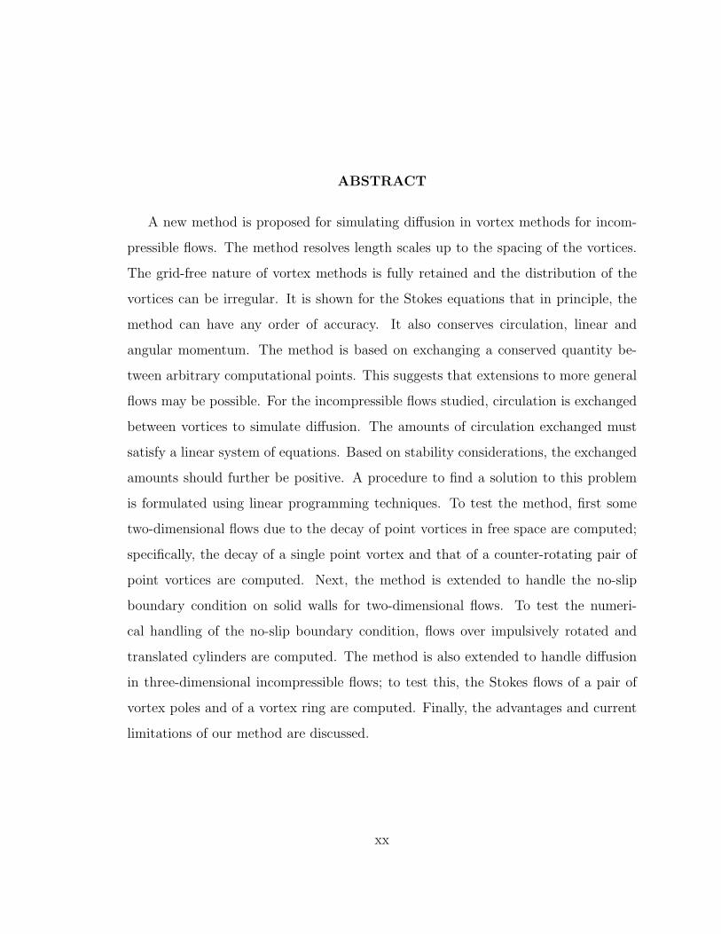
ABSTRACT

A new method is proposed for simulating diffusion in vortex methods for incom-

pressible flows. The method resolves length scales up to the spacing of the vortices.

The grid-free nature of vortex methods is fully retained and the distribution of the

vortices can be irregular. It is shown for the Stokes equations that in principle, the


















xx

CHAPTER 1

INTRODUCTION

A number of engineering problems involve flows of gases or liquids over solid

bodies. For example: air flows over cars and aeroplanes; wind blowing over bridges

and buildings; sea waves slashing against the supporting columns of an off-shore

oil rig and many more. Often these flows do not follow the contour of the solid

surface completely, but separate from it, creating a wake such as behind a ship.

Such separated flows are difficult to handle by conventional numerical schemes. The

objective of this work is to develop a numerical procedure to solve such flows. It

is based on determination of the vorticity, defined as the curl of the flow velocity.

According to Stokes [225] vorticity is the twice the local angular velocity of the fluid

if it moves as a solid body.

The main reason to base the numerical method on the vorticity is that, typically,

only a small portion of the flow contains vorticity. This can lead to significant savings

in storage and computational effort. Our numerical method will compute the evo-

lution of vorticity using a Lagrangian approach, in which the computational points

follow the motion of the fluid. Such a method is commonly called a vortex method,

and the computational points are the vortices.

Vortex methods can offer significant advantages for the computation of separated

flows:

• We need to describe only the small portion of the flow region where vorticity

occurs. Typical conventional methods must resolve the whole flow.

• In our implementation no grid is required. This makes it easier to handle flows

around complicated geometries.

1

2

• If the vorticity separates from the solid surfaces, the vortices follow that motion,

so that numerical resolution is maintained.

• In a conventional computation, the motion of the vorticity must be found by

numerical approximation on a fixed grid, which can induce significant numerical

dissipation. A vortex method avoids this since the vortices follow the motion

of the fluid.

• In the computation of the velocity field from the vorticity, mass conservation can

be satisfied exactly; see, for example, Van Dommelen & Rundensteiner [233].

Gresho [98, 101] has shown that mass conservation can be a cause of difficulty

in other computations.

• In external flows, most methods need to restrict the computational domain

artificially to a finite size. But as long as the vorticity remains limited to a

finite region, vortex methods need not.

These advantages are most often critical for high Reynolds number flows, which

are commonly separated. An important concern at high Reynolds numbers is that

the numerical dissipation should not overwhelm the natural viscous diffusion process

and destroy the small scale features. Such requirements make vortex methods a

natural choice. Yet, the implementation of vortex methods is not simple. The two

main physical processes that must be represented numerically are convection of the

vorticity by the velocity field and diffusion due to viscosity. Each has its difficulties.

For convection of the vortices, the velocity field can in principle be found from

the Biot-Savart law [14]. Such a velocity field implicitly satisfies mass conservation.

However, the computational effort required to evaluate it directly is high; it is propor-

tional to the square of the number of vortices. Fast algorithms have been developed

to do it with much less effort. Van Dommelen & Rundensteiner [233, 240] developed

3

the first ‘solution adaptive’ fast method that could efficiently handle the sparse and

complex vorticity distributions of high Reynolds number separated flows. An earlier

non-adaptive routine was given by Greengard & Rokhlin [97]. Even faster algorithms

are available now [2, 5, 10, 36, 74].

However, representing diffusion is a more difficult problem; one of the main diffi-

culties is the chaotic distribution of the vortices. It is this difficulty that is the main

topic of this thesis. In this thesis, we have developed an accurate mesh-free procedure

to overcome that difficulty. We next discuss the importance the mesh-free property

in Lagrangian methods.

1.1 The need for mesh-free Lagrangian methods

One of the major difficulty in mesh-based computations of high Reynolds number

separated flows around complex geometries like multi-element airfoils or even more

complex geometries like fighter aircrafts, is to generate an effective mesh to solve

the governing flow equations. The common strategy of generating a mesh with fine

resolution near solid walls may not be adequate in high Reynolds number separated

flows. The reason is that the steep flow gradients, such as in boundary layers, do not

always occur only normal to a solid wall. For example, to compute the flow around

an impulsively started cylinder, the mesh does not only need to be refined normal

to the cylinder wall. When separation occurs, sharp gradients also develop in the

direction along the wall. Van Dommelen & Shen [241] showed that in fact very fine

resolution is required in the direction along the wall to resolve the rapid evolution

of the vorticity layers in that direction. More often the steep flow gradients also

occur due to separated vorticity fields, like the forebody vortices from an aircraft, for

example. It is very difficult to predict a priori the evolution of the separated vorticity

fields.

4

An accurate representation of the separated vorticity fields is crucial to determine

the aerodynamic forces on bodies accurately, yet it is very difficult to accurately

resolve the separated vorticity fields using a mesh. At high Reynolds numbers, the

numerical diffusion due to insufficient resolution could overwhelm the actual diffusion,

and hence the separated vorticity fields will be diffused erroneously; this will result

in large errors in the computed aerodynamic forces on vehicles such as fighter planes

and cars. It can cause difficulties for computing airplane control forces when the

inaccurate separated vorticity from the main wing interacts with the tail surfaces.

On the other hand, since the vortex methods are based on following the vorticity,

they provide excellent adaptive resolution of the separated vorticity fields.

In vortex methods, the convection of vortices can be achieved using mesh-free

algorithms, as mentioned earlier. However, the diffusion of vortices must also be

handled in a mesh-free manner to avoid the difficulties of mesh-based computations,

and this is a more difficult problem. One of the main difficulties is the chaotic

distribution of the vortices. High Reynolds number flows are characterized by a

strong mixing of the vortices, and a regular vortex distribution is almost impossible

to maintain.

Some previous attempts to deal with this difficulty have been based on interpo-

lating to a mesh for at least some of the computation (section 1.2). However, this

loses a significant part of the advantage that a Lagrangian computation attempts to

achieve over conventional computation: it is very hard to produce efficient meshes for

complex geometries, especially for separated flows where they need to resolve sharp

gradients that are not aligned with the boundaries. Further, using a mesh introduces

interpolation errors between the mesh and the vortices, and the resulting wide variety

of errors tends to make the final accuracy uncertain.

Alternate approaches to deal with the irregular vortex locations restore order

periodically, by periodically selecting a new set of vortices with strengths found by

5

interpolation from the previous set (subsections 1.3.3 and 1.3.4). One difficulty is

that the generation of an effective new vortices distribution is not really different

from generating a mesh; another difficulty is that at high Reynolds numbers, to be

truly effective, the regeneration has to be done frequently. This requires again effective

solution adaptive meshes, which would be a very difficult problem for “real life” high

Reynolds number separated flows about complex configurations. The interpolation

errors and trade-offs in choosing the times at which to redefine the vortex distribution

again introduce considerable uncertainty about the optimal procedure and the final

errors.

In order to actually achieve the advantages that a Lagrangian computation

promises, such as the elimination of the mesh generation problem and the accu-

rate representation of separation processes and separated vorticity without excessive

mesh points, better approaches are needed. Those approaches must directly handle

the irregular vortex distribution produced by high Reynolds number flows. A number

of methods that can do this have been proposed (subsections 1.3.1, 1.3.2 and 1.3.5),

of which the “random walk” method of subsection 1.3.1 has without doubt turned

out to be the most effective. However, although this method works (e.g. see figure

8.22), in practice it is quite inaccurate. This may in part be due to the fact that the

random walk method does not satisfy the various physical conservation laws exactly.

Furthermore, the method is of a statistical nature, which means that the results are

not easily reproducible, and the errors may be even larger if you happen to be unlucky.

In parameter studies, it is very difficult to separate the effect of the parameters from

the random errors. There is further no obvious way to improve the order of accuracy

of the method.

In this thesis we will propose another method to deal with chaotic vortex distribu-

tions. It could be called a “computed finite difference” method, since we compute the

equivalent of a finite difference formula for the diffusion of each vortex at each time.

6

However, since the effect of the finite difference formula is to redistribute part of the

strength of each vortex among its neighbors, we call it the “Redistribution Method”.

We will show that this method can be implemented efficiently and is significantly

more accurate than the random walk method. It also does not have the inherent

limitations in order of accuracy of the random walk method. In the following, we

briefly describe the various existing methods for handling diffusion. We will show

that these existing methods cannot handle our requirements for a mesh-free accurate

procedure. Finally, we will introduce our new method that can.

1.2 Hybrid methods for diffusion

One possible approach to handle diffusion in vortex methods is to use a conven-

tional mesh. Since this combines both vortex and mesh based approaches it is called

a hybrid method. The basic procedure is the following: First, the vorticity at mesh

points is determined from the vortices using some interpolation scheme. Then the

diffusion equation is solved on this mesh to obtain diffused vorticity values at the

mesh points. After this, the strengths of the existing vortices can be updated using

the diffused vorticity values of the mesh points and the mesh can be discarded [92];

alternately, the existing vortices can be removed and new ones created at the mesh

points [40, 138, 139, 163].

One of the main reasons for using a mesh is the convenience in evaluating the

spatial derivatives of the vorticity or any other flow variable. This is also one of the

reasons for using a mesh in the Vortex-In-Cell method (VIC) [56, 61, 76] and the

Particle-In-Cell (PIC) type methods [108, 158]; in both these methods the numerical

diffusion is a major disadvantage [30]. Similarly, using a mesh for diffusion has the

disadvantage of high numerical diffusion due to the interpolations. This is not desir-

able for high Reynolds number flows or other situations where small scales need to

7

be resolved. It is also difficult to ensure that the interpolated vorticity satisfies the

governing equations and conservation laws.

Apart from the above methods, there is another hybrid approach to handle dif-

fusion. In this approach the flow domain is divided into viscous regions adjoining

the solid boundaries (usually, the boundary layers) and convection dominated re-

gions outside it. In each of those regions, different formulations of the Navier-Stokes

equations [179] can be used; or approximations to the Navier-Stokes equations may

instead be used. Any of the above equations can be solved using vortices or a mesh

or a combination of both. This opens the way for numerous variations, some of which

can be found in [5, 52, 55, 66, 103, 111, 207, 216].

The motivation for using these methods is their ability to handle the viscous

regions accurately and efficiently [38, 65, 66, 111]. For example, the no-slip boundary

condition can be handled accurately [55, 103]. Moreover, efficient numerical schemes

can be used in various regions; typically, a finite difference or a finite element scheme

is chosen.

However, dividing the flow domain into different regions has an inherent difficulty:

it may not be easy to formulate appropriate conditions at the boundary between the

regions [66, 103, 111, 206]. Some authors consider the boundary layer equations to

be simpler to use in the viscous regions instead of the full Navier-Stokes equations

[4, 216]; the difficulty here is that the boundary layer equations could quickly become

invalid. Such is the case whenever unsteady boundary layer separation occurs, as

shown by Van Dommelen and Shen [241, 243].

To summarize, many of the difficulties of the above approaches are caused by the

mesh; in particular, the high numerical diffusion is a major disadvantage. In addition,

it may be difficult to generate a mesh for flow around a complicated geometry; and

in an external flow, it may be difficult for a mesh to exactly represent an infinite

8

domain. All these difficulties are eliminated in mesh-free methods; we will discuss

such methods in the next section.

1.3 Lagrangian methods for diffusion

A number of numerical schemes model diffusion in vortex methods without using

a mesh. Such methods are based on the Lagrangian approach and use vortices only.

Often the vortices are unevenly and sparsely distributed; this makes it difficult to

compute vorticity gradients and to represent diffusion in regions depleted of vortices.

We will describe ways to handle such difficulties while discussing various methods.

Some of the current methods model diffusion by changing the parameters of the vor-

tices: their positions (Random Walk method); their sizes (Core Expansion method);

or their circulations (Deterministic Particle method). Other methods model diffusion

using smooth interpolants to approximate the actual vorticity distribution (Smoothed

Particle Hydrodynamics method and Fishelov’s method); or even by altering the char-

acter of the diffusion process (Diffusion Velocity method). We will briefly review the

above methods in the following sections.

1.3.1 Random walk method

The random walk method to model the diffusion of vorticity was first proposed

by Chorin [54]. To simulate the diffusion of vorticity in vortex methods, the positions

of the vortices are given random displacements (a random walk) [48]. These random

displacements have zero mean and a variance equal to twice the product of the kine-

matic viscosity and time step. The basic idea of the random walk method is that the

random displacements spread out the vortices like the diffusion process spreads out

the vorticity.

9

Several studies investigate the theoretical and numerical aspects of the random

walk method: Marchioro & Pulvirenti [144], Goodman [90], and Long [135] have

shown that for flows in free-space, the random walk solution converges to that of the

Navier-Stokes equations as the number of vortices is increased. However, there are

no convergence studies for flows involving solid walls. Puckett [178] gives a survey

of the elements of vortex methods; in particular, he discusses in detail the random

walk method and its convergence. Chang [41] discusses how to incorporate the ran-

dom walk method in Runge-Kutta time-stepping schemes. Ghoniem & Sherman [85]

studied ways of handling the boundary conditions. They also develop a ‘gradient ran-

dom walk’ method [51, 205] in which the computational points transport derivatives

of vorticity instead of the vorticity itself; they show that this procedure produces

smoother vorticity distribution than the random walk method.

The random walk method has been used extensively. Here we will mention only

some of the applications: Chorin applied the random walk method for simulating

flows around cylinders [49, 54] and flat plates [49, 50, 52]. Shestakov [207] has used

the random walk method for flow inside a driven cavity. McCracken & Peskin [149]

have studied the blood flow through heart valves using the random walk method.

Ghoniem [84, 86], Sethian [200] and Majda & Sethian [142] have applied the random

walk method to problems in combustion; more recently, the random walk method

has been used in combustion problems by Melvin [154], Pindera [173], Caldaza [34]

and Song [211]. Sod [210] has used random walk method to study the interactions of

shock waves with boundary layers. Cheer [42, 43] has implemented the random walk

method for flows over a cylinder and an airfoil. Van Dommelen [213, 237, 238] studied

flows over impulsively started cylinders, pitching airfoils, jets and cavities. Ghoniem

& Cagnon [83] studied the entry flow in a channel and the flow over a backward-facing

step using the random walk method. Sethian & Ghoniem [199] studied convergence

for a backward-facing step numerically. Martins and Ghoniem [146] have applied the

10

random walk method to simulate the intake flow in a planar piston-chamber device.

Smith & Stansby [214, 215] have studied flows over impulsively started cylinders.

Wang [245] studied various flow control techniques to avoid the dynamic stall of

airfoils. Seo [198] has applied the random walk method to flows over translating,

oscillating and pitching two-dimensional bodies of arbitrary shape. Tiemroth [221]

and Vaidhyanathan [228] have applied the random walk method to study flows over

submerged and floating bodies including free-surface interactions. Summers [220] has

applied the random walk method to Falkner-Skan boundary layer flows. Chui [58] used

the random walk method to study thermal boundary layers. Baden & Puckett [12],

and Choi, Humphrey & Sherman have applied the random walk method to compute

the flow inside square cavities. Lewis [128] has used the random walk method for flow

over airfoil cascades.

The random walk method has some advantages: it is simple to use; and it can

easily handle flows around complicated boundaries. The method conserves the total

circulation.

However, the random walk method also has some major disadvantages. First, it

does not exactly conserve the mean position of the vorticity in free space. Next, the

computed solutions are noisy due to the statistical errors. In flow control studies,

the statistical errors could mask the effects of varying the control parameters. The

statistical errors can also cause symmetric flows to turn asymmetric erroneously. To

reduce the statistical errors requires a very large number of vortices.

Many investigations have studied how the errors in the random walk computations

vary with the number of vortices. Milinazzo & Saffman [155] tested the random

walk method for the case of an initially finite region of vorticity in an unbounded

domain. They corrected for the error in the mean position, but found that the error

in computed mean size of the vortex system is proportional to the inverse square root

of the number of vortices N . If the initial vorticity inside the region is constant, the

11

number of vortices must be increased with Reynolds number to keep the relative error

in change in size constant at finite times. Roberts [182] showed that if the relative

error in size itself is of importance, higher Reynolds numbers do not require additional

vortices. In fact, the number of vortices can be reduced if the initial data represent

the initial mean size accurately. Fogelson & Dillon [79] have used a simplified one-

dimensional version of the problem to study the question how much smoothing should

be applied to the random walk results. They found that convergence occurs when

the random walk solution is smoothed over a distance that is large compared to the

point spacing. Their results show that still a very large number of vortices is needed

to improve the accuracy of the random walk method.

From such studies, it follows that the random walk method needs a very large

number of vortices for accurate simulations. Correspondingly, the amount of work

to convect all the vortices also becomes large. In addition, since the method is not

deterministic, the random errors cause difficulties in the physical interpretation of the

results. As an alternative to random walk, a number of deterministic methods have

been proposed; we will discuss such methods in the following.

1.3.2 Core expansion method

Another procedure to model diffusion is the core expansion method proposed

by Leonard [126]; in two dimensions, the core of a vortex is the characteristic size

of that vortex. In the core expansion method, the core of each vortex is allowed

to expand according to the diffusion equation. Earlier Kuwahara & Takami [121]

have used expanding vortex cores to compute the motion of a vortex sheet in an

inviscid fluid. However, their objective was not to model diffusion but to eliminate

the large velocities induced by point vortices. For that, they use the velocity field of

a diffusing vortex instead of the velocity field of a point vortex; they do point out

that the viscosity is an artificial viscosity and that its value must be chosen as small

as possible.

12

The core expansion method has been used to simulate several flows. Rossi [186]

has used the method to simulate wall jets. Zhang & Ghoniem [252] have applied

the method to buoyancy-driven plumes. Chua [57] and Leonard [124] have used the

method to simulate the collision of vortex rings. Meiburg has used the method for

simulating diffusion flames [152] and mixing layers [153]. Nagano, Naita & Takata

[162] have used the method for flows over rectangular prisms.

The core expansion method is exact for the Stokes equation. However, Greengard

[96] has shown that it cannot model convection correctly when applied to the Navier-

Stokes equations. The error in convection arises if the vortices become finite in size

compared to the length scale of the flow. To reduce the convection error, Rossi [185]

proposed the ‘corrected core spreading vortex method’ in which the large vortices

are split into smaller ones; however, the number of vortices grows exponentially in

time. Also, the number of smaller vortices, their sizes, and the frequency of vortex

splitting are critical control parameters that must be chosen apriori; these are sources

of uncertainty in a computation.

1.3.3 Deterministic particle method

A deterministic method to simulate diffusion has been developed by Raviart [180],

Choquin & Huberson [45], and Cottet & Mas-Gallic [64]. They use viscous/inviscid

splitting of the vorticity equation and then solve the diffusion equation exactly using

the fundamental solution of the heat equation. Recently the ‘Deterministic Particle

(or Vortex) Method’ has been developed along different lines by Degond & Mas-

Gallic [72], and Mas-Gallic & Raviart [147]. The basic ingredients in this approach

are: (a) to consider the strength (circulation) of each particle (vortex) as an unknown

coefficient that changes with time due to diffusion effects, (b) to approximate the

diffusion operator by an integral operator, and (c) to discretize the integral using the

particle positions as quadrature points.

13

In practice, such methods start out with a fixed number of particles, distributed

uniformly over the domain, each with a prescribed initial strength [119, 170]. Changes

in the particle strengths then simulate the diffusion effects through a system of ordi-

nary differential equations [119, 170]. These changes can be interpreted as changes in

the strengths of particles due to the neighboring particles. For this reason, Winckel-

mans [247] and Koumoutsakos [119] call the deterministic particle method the ‘Par-

ticle Strength Exchange’ method (PSE)

Choquin & Lucquin-Desreux [46] have investigated the accuracy of the method

for axisymmetric vorticity distributions in two-dimensions. Huberson, Jolles & Shen

[111] applied it to a concentrated vortex in a shear flow. Choquin & Huberson [45]

studied the Kelvin-Helmholtz instability of a shear layer. Winckelmans & Leonard

[247] have used the PSE scheme to study the fusion of vortex rings. Cottet [67] and

Mas-Gallic [148] have extended the deterministic particle method to problems with

boundary conditions. Pepin [170] used the local vorticity flux to adjust the strength

of the vortices near a boundary. Koumoutsakos, Leonard & Pepin [118] describe the

no-slip boundary condition in terms of the vorticity flux based on the fundamental

solution of the heat equation. Koumoutsakos & Leonard [117] have applied the scheme

to impulsively started and stopped flows around translating and rotating cylinders for

Reynolds numbers from 40 to 9500; further computations of the flow over a cylinder

include that of Cottet [65, 66], Guermond, Huberson & Shen [103], and Huberson,

Jolles, & Shen [111]. Shen & Phuoc Loc [206] have simulated the flow over an airfoil

using PSE.

However, the PSE method has some disadvantages. The vortex size must be

sufficiently large that there is a significant overlap of vortices. This requirement re-

duces the ability of the method to resolve the smallest scales; for example, the Stokes

layer generated by an impulsive change in boundary conditions is numerically dif-

fused over a significant number of vortices away from the boundary. Further, the

14

PSE method requires that the uniformity of the particle distribution be periodically

restored [65, 66, 111, 119, 170]. The uniformity is restored using a mesh [119, 170] and

this makes it difficult to handle flows over complicated geometries. For flows with sep-

arated vorticity, the mesh would have to be adaptive to be effective, greatly increasing

the difficulties. Even then, the interpolation to the mesh introduces significant errors

and inaccuracies.

1.3.4 Fishelov’s method

A method with properties similar to the particle strength exchange (PSE) scheme

was derived by Fishelov [78]. She convolves the spatial derivatives in the vorticity

equation with a smoothing function and then transfers the derivatives on to that

function. This procedure of using smoothing functions to compute spatial derivatives

is similar to the procedure used in the Smoothed Particle Hydrodynamics (SPH)

method [22, 25, 88, 140, 157, 158]. Fishelov showed that the L2 norm of the vorticity

does not increase in her method, implying stability, at least for the heat equation,

provided that the Fourier transform of the smoothing function is nonnegative. This

method readily extends to higher order of accuracy. With proper discretization, it

can be made to conserve vorticity exactly. Recently, Bernard & Thomas [23, 24] have

applied this method to boundary layers over flat plates.

However, Fishelov’s method requires periodic remeshing and particle overlap to

maintain accuracy [23, 24] like the PSE scheme. It has therefore similar disadvantages.

1.3.5 Diffusion velocity method

The basic idea of the diffusion velocity method is to handle diffusion as a part of

the convection process. To do that an artificial velocity field is defined to represent

the diffusion process. Golubkin & Sizykh [89] and Ogami & Akamatsu [165] identify

the ‘diffusion velocity’ by absorbing the diffusion term into the convection term in

the vorticity equation. Kempka and Strickland [116] derive the same expression for

15

the diffusion velocity in a different way. It turns out that the diffusion velocity is

proportional to the ratio of the vorticity gradient to the vorticity. The diffusion

velocity is then added to the incompressible velocity field to convect the vortices.

Ogami & Akamatsu [165] applied this method to the one-dimensional Stokes flow

of an initially uniform vortex patch. Strickland, Kempka & Wolfe [218] have applied

it to several simple one-dimensional problems involving solid walls. Clarke & Tutty

[59, 227], and Huyer & Grant [112, 113] have used this method for the flow over a

cylinder and an airfoil. Recently, Ogami & Cheer [164] have extended the diffusion

velocity method [165] to compressible flows.

The diffusion velocity method is mesh-free since the vorticity gradients are evalu-

ated as in the SPH method mentioned in the subsection 1.3.4. However, the definition

of the diffusion velocity gives rise to inherent problems: special care is needed in re-

gions where the vorticity vanishes and also where vorticity gradients are large. The

method also requires a large number of overlapping vortices for accurate simulations

due to large variations in the diffusion velocity in different parts of the flow. Kempka

and Strickland [116] noticed that the diffusion velocity is not divergence free. They

interpret the effect of this nonzero divergence as a change in the size of the vortices.

They show that the accuracy of the diffusion process can be improved by modifying

the size of the vortices according to the nonzero divergence. However, such modifi-

cations are not easy to handle and lead to severe restrictions on the size of the time

step [116]. Further, the overlap of the vortices must be carefully monitored similar

to PSE and Fishelov’s methods.

Finally, the observations of Degond & Mustieles [71] may be noteworthy: The

diffusion velocity may become infinite in regions of vanishing vorticity or large vor-

ticity gradients. However, for numerical implementation the diffusion velocity has to

be finite; this creates a ‘diffusion front’ and could lead to numerical instability. In

fact, their one-dimensional computation of the diffusion of an initially smooth vor-

16

ticity field shows numerical oscillations in the regions of vanishing vorticity. They

also point out that this method may be less accurate and more expensive than other

methods for the Navier-Stokes and the heat equations. However, it may be suited to

problems in the kinetic theory of plasma physics.

1.3.6 Free-Lagrange method

Another deterministic vortex method is the free-Lagrange method developed by

Borgers & Peskin [28], Rees & Morton [181], Russo [188], and Trease, Fritts & Crowley

[224], among others. The basic idea is to construct a finite difference scheme for the

derivatives using the Voronoi diagram [161] of the vortices. The computational effort

to construct the Voronoi diagram is of the the same order as that of the convection

of the vortices using fast algorithms [36, 97, 233] for example. Russo [188] has shown

that the method does conserve vorticity and angular momentum but it is only weakly

first-order consistent. Borgers and Peskin [28] have shown that the method requires

a uniformity condition for the distribution of the points.

1.4 The vorticity redistribution method

In the previous section we discussed several Lagrangian methods for diffusion,

each of which has its own characteristics. Each of those methods has difficulty ei-

ther in handling diffusion accurately or in handling the complex boundary conditions

and vorticity fields in many practical flows: The random walk method requires a

very large number of vortices for accurate simulations. The PSE method and Fish-

elov’s method require remeshing and vortex overlap to maintain the accuracy of the

numerical computations. However, remeshing procedures for flows over complicated

boundaries or with complex vorticity fields and maintaining particle overlap in flows

with strong convection are difficult. The core expansion method does not represent

17

the convection process correctly for the Navier-Stokes equations. Finally, in the dif-

fusion velocity method, evaluating the diffusion velocity accurately is difficult.

The above difficulties suggest the need for an accurate mesh-free method to han-

dle diffusion. The vorticity redistribution method developed in this work addresses

the above difficulties: Unlike the random walk method, the vorticity redistribution

method is deterministic and implicitly maintains the vorticity conservation laws.

Therefore, our method does not need as many vortices as the random walk method

for the same accuracy. Our method has the advantage over the PSE and Fishelov’s

methods in that it is mesh-free. This mesh-free property of our method provides a sig-

nificant advantage to compute flows over complicated geometries accurately. Another

difficulty with the PSE and Fishelov’s methods is the resolution of sharp gradients

in the flow; their resolution is asymptotically limited to a size that is asymptotically

much larger than the average spacing of the particles, (see section 9.1). However,

the resolution in our method is of the order of the average spacing of the particles.

We also do not have difficulty in representing convection correctly, unlike the core

expansion method. Finally, our method does not face the difficulties of the diffusion

velocity method since we do not use the diffusion velocity in our computations.

Next, we will describe the basic idea of the vorticity redistribution method. The

vorticity redistribution method is similar to the deterministic particle methods [72, 78]

in that it changes the strengths of the vortices to simulate diffusion: fractions of the

strength, or circulation, of each vortex are moved to neighboring vortices in order to

produce the correct amount of diffusion. However, while the deterministic particle

methods use simple approximations to find the amounts of circulation to move, instead

in section 4.1 we will formulate a special system of equations for it. Also, unlike the

deterministic particle methods, the maximum distance that the circulation of a vortex

is allowed to move during a time-step is restricted to a chosen distance of the order

of the point spacing, rather than large compared to it. This allows scales up to the

18

point spacing to be resolved. Unlike free-Lagrangian methods, no partitioning of the

domain is attempted; instead, all available vortices within the allowed distance are

included in the discretization.

The key question is to choose the fraction of the circulation of each vortex that

is moved (redistributed) to each neighboring vortex. This choice determines the

accuracy of the approximation, its stability, and its conservation properties. We will

formulate a system of equations from which the redistribution fractions can be found

in section 4.1. As will be seen in section 4.2, the equations of this system takes the

form of localized conservation laws. This system can be extended to any order of

accuracy. A uniform distribution of vortices is not required; however, for uniformly

distributed points our method is equivalent to a finite difference scheme. Positivity of

the solution of the system is enforced to ensure stability. We use a solution procedure

that is guaranteed to find a positive solution to the system of equations, if one exists.

If there is no acceptable solution, we add new vortices until there is one.

Fundamentally, our procedure differs from the usual particle methods by sepa-

rating the computation of the vorticity into two distinct steps: (a) determination of

vortex strengths from the localized conservation laws; (b) reconstruction of the vor-

ticity field by convolution. This separation allows us to achieve any chosen order of

accuracy regardless of the geometry of the vortex distribution. However, unlike the

particle methods, and other numerical methods, in our scheme an individual vortex

strength has no identifiable meaning. It is the combination of nearby vortex strengths

and positions that determines the local solution. In chapter 9, we discuss the practical

implications of these differences.

We next describe the organization of this thesis.

19

1.5 Organization of the thesis

In chapter 2 we review the governing flow equations and vorticity conservation

laws. In chapter 3 we describe vortex methods in general. In chapter 4 we formulate

our new ‘vorticity redistribution method’. In chapter 5 we establish the convergence

of the vorticity redistribution method for the Stokes equations. In chapter 6 we

describe the numerical implementation of the vorticity redistribution method. In

chapter 7 we apply the method to flows in free space. We first compute the flow due

to the the decay of point vortices in two-dimensional free space and then compute

two Stokes flows in three-dimensional free space. In chapter 8 we apply the method

to compute two-dimensional flows over solid walls. We first apply the method to

compute axisymmetric flows over circular cylinders. Next, we compute the more

complicated case of an impulsively translated circular cylinder for a wide range of

Reynolds numbers. We present the streamlines, velocity fields, vorticity fields, and

the drag coefficients. We validate our results against boundary layer computations

and other numerical computations. We also compute the interaction of a vortex

pair with a circular cylinder to illustrate the simplicity of our method. In chapter 9

we discuss the advantages of the redistribution method compared to other particle

methods. Finally, in chapter 10 we give our conclusions.

CHAPTER 2

GOVERNING EQUATIONS

In this chapter we review the flow equations that describe the evolution of vorticity

and velocity. The conservation laws of vorticity are also reviewed.

2.1 Navier-Stokes equations

Consider the two-dimensional flow of a homogenous and incompressible fluid. The

density and the viscosity of the fluid are both assumed to be uniform. We assume

that any body forces on the fluid are derived as a gradient of a scalar function. The

governing equations for the motion of the fluid are the conservation of mass and linear

momentum [14].

The mass conservation equation is

∇ · ~u = 0 , (2.1)

where ~u is the velocity and ∇ is the gradient operator. We also denote ~x = (x, y) to

be any point in the plane and x and y to be the unit vectors along the axes.

The linear momentum conservation for a Newtonian fluid is given by the Navier-

Stokes equations [14],

∂~u

∂t+ ~u · ∇~u = −1

ρ∇p + ν∇2~u + ~F , (2.2)

where t is time; p is mechanical pressure; ~F is body force per unit mass of the fluid;

ν is kinematic viscosity, defined as the ratio of the dynamic viscosity and the density

of the fluid and ∇2 is the Laplacian operator.

20

21

The equation for the the evolution of vorticity can be derived from the Navier-

Stokes equations (2.2). To do that, we first define the vorticity ~ω to be the curl of

the flow velocity,

~ω ≡ ∇× ~u . (2.3)

For two-dimensional flows, the vorticity vector is normal to the plane of the flow; that

is, ~ω = ωz, where z = x × y is an unit vector normal to the plane. The vorticity

equation is obtained by taking the curl of (2.2) and it is given by:

∂ω

∂t= −~u · ∇ω + ν∇2ω . (2.4)

The physical interpretation of each of the terms in the vorticity equation (2.4)

is the basis for the formulation of vortex methods. On the right hand side of (2.4)

the first term represents the transport of vorticity due to the velocity (convection

process), and the second term represents the change in vorticity due to viscosity

(diffusion process) [14]. Truesdell [225] has described the convection and diffusion

processes in detail from a kinematic point of view.

To solve (2.4) for a particular problem, initial and boundary conditions must be

specified. The initial vorticity field may be prescribed or it may also be derived as the

curl of a specified initial velocity field [179]. Boundary conditions must be specified

when there are boundaries in a flow. On a solid impermeable boundary, the velocity

of the fluid on the boundary must be the same as the velocity of the boundary itself

[14],

~u(~s, t) = ~us(~s, t) , (2.5)

where ~s is any point on the boundary and ~us is the velocity of the boundary. Notice

that the boundary condition (2.5) is in terms of velocity and not vorticity; we will

discuss the handling of this boundary condition in section 6.3. Further, in many

applications the flow domain is unbounded and at large distances the velocity is

either uniform or vanishes; hence the vorticity vanishes at large distances also.

22

A number of theoretical studies have investigated the validity of the vorticity

formulation of the Navier-Stokes equations. McGrath [150] showed that for flows

in free space the vorticity equation has an unique solution for any finite time if

the initial vorticity is smooth (twice differentiable). A similar result for singular

initial vorticity distributions (that are absolutely integrable) has been established by

Benfatto, Esposito & Pulvirenti [21], Giga, Miakawa & Osada [87], Ben-Artzi [20, 31]

and Kato [114].

Guermond & Quartapelle [102] and Quartapelle [179] have shown that the the vor-

ticity formulation is equivalent to the velocity-pressure form of Navier-Stokes equa-

tions. Gresho [98, 99, 100] discusses a number of theoretical and computational issues

for the vorticity formulation for incompressible flows.

Vortex methods are based on the Lagrangian approach in which the “fluid parti-

cles” are used as the basic computational elements [14]. Here the fluid particles are

understood to be small volumes of fluid. To be precise, particles are volumes of fluid

that are much smaller than all relevant length scales of the flow but still much larger

than the molecular size and mean free-path length. The time derivative following a

fluid particle is defined asD

Dt≡ ∂

∂t+ ~u · ∇ . (2.6)

In terms of this “Lagrangian time-derivative”, we can rewrite the vorticity equation

(2.4) as [14],Dω

Dt= ν∇2ω . (2.7)

According to (2.7), the vorticity of a fluid particle changes only due to diffusion. In

inviscid flows (ν = 0) the vorticity of a fluid particle does not change [14, 137]; this

result is very useful in formulating vortex methods described in the next chapter.

However, the vorticity equation is only one equation for three unknowns, ω, u,

and v, and we need equations to determine the velocity field also; we will formulate

the equations for the velocity field next.

23

2.2 Velocity field

The velocity field determines the motion of the vorticity field. On the other hand,

it turns out that we can find the velocity field from the vorticity field; in the following,

we describe this.

The mass conservation equation (2.1)

∇ · ~u = 0 , (2.8)

can be satisfied using a scalar function ψ(~x, t) called the stream function [14] such

that

∇× ψz = ~u . (2.9)

Equivalently, (2.9) implies that the velocity components (u, v) are given by,

u =∂ψ

∂y(2.10)

−v =∂ψ

∂x. (2.11)

We substitute (2.10) and (2.11) in the definition of vorticity (2.3) and obtain the

following Poisson equation for the stream function,

∇2ψ = −ω . (2.12)

We can solve (2.12) to find the stream function and then the velocity field using

(2.9). A standard approach to solve the Poisson equation (2.12) is the Green’s function

method [13, 95]. Using this method, for flows in free space (no boundaries) we can

obtain ψ from (2.12) as,

ψ(~x, t) =∫ ∫

G(~x; ~x′) ω(~x′, t) dx′ dy′ (2.13)

≡ G ∗ ω ,

24

where ∗ denotes the convolution operation [13] and G is the free space Green’s func-

tion, also known as fundamental solution, of the Laplace equation. This Green’s

function satisfies

∇2~xG(~x; ~x′) = δ(~x− ~x′) , (2.14)

where δ(·) is the two-dimensional Dirac delta function; and ∇2~x is the Laplacian

operator in which the derivatives are with respect to ~x. The actual form of G is

[13, 95],

G(~x; ~x′) =1

2πln(| ~x− ~x′ |) . (2.15)

Using (2.13) in (2.9), we obtain the velocity field

~u(~x, t) =∫ ∫

~K(~x; ~x′) ω(~x′, t) dx′ dy′ (2.16)

≡ ~K ∗ ω ,

where ~K is given by

~K(~x; ~x′) = ∇~x ×G(~x; ~x′)z (2.17)

=1

2π | ~x− ~x′ |2

y − y′

x′ − x

. (2.18)

The equations (2.16) and (2.18) for the velocity are known as the Biot-Savart law

[109, 126]. The function ~K is also called the kernel [11], the Biot-Savart Kernel [109]

or the velocity kernel [17].

The velocity given by (2.16) is for free space flows since we used the free space

Green’s function in (2.13). For flows over solid boundaries, this velocity can be

corrected to satisfy the boundary condition (2.5); we will describe that in section 6.3.

The vorticity equation (2.7), the velocity equation (2.16), the initial condition

and the boundary conditions together describe the evolution of the vorticity. Next

we review the conservation laws derived from the vorticity equation.

25

2.3 Vorticity conservation laws

The vorticity conservation laws can be viewed as constraints on the motion of the

vorticity. These conservation laws can be used to monitor the accuracy of numerical

computations or even to construct accurate numerical schemes.

The conservation laws can be derived from the vorticity equation. Poincare [174]

derived the conservation laws for two-dimensional flow of a homogenous incompress-

ible viscous fluid in free space; they are,

d

dt

∫ ∫ω(~x, t) dx dy ≡ dΓ

dt= 0 (2.19)

d

dt

∫ ∫~xω(~x, t) dx dy = ~0 (2.20)

d

dt

∫ ∫~x · ~x ω(~x, t) dx dy = 4 ν Γ , (2.21)

where ν is the kinematic viscosity of the fluid and Γ is the total circulation. Howard

[110] showed that these are the only conservation laws for such flows; they are also

the conservation laws for the vorticity equation without convection (Stokes equation).

Truesdell [225] derived various laws for the average motion of vorticity in flows over

solid boundaries.

The above conservation laws have the following interpretation [14, 122]: The first

equation (2.19) states that the total circulation Γ is conserved. Equation (2.20)

implies that the average position of the vorticity (center of vorticity) does not change

in time. Equation (2.21) is a measure of how fast a vortical region expands. For

flows in which the linear and angular momenta are bounded, the equations (2.20)

and (2.21) can also be interpreted as conservation of those two momenta respectively

[122].

26

2.4 Summary

In this chapter, we derived the governing equations for velocity and vorticity; and

we also discussed the boundary conditions on solid walls and vorticity conservation

laws. Our next objective is to solve numerically the governing equations for the vortic-

ity and velocity derived in this chapter. Vortex methods are well suited to accomplish

this objective since they offer a number of advantages listed in the introduction; we

will describe the vortex methods in the next chapter.

CHAPTER 3

VORTEX METHODS

Vortex methods are numerical methods to solve the vorticity equation. In this

chapter we will briefly describe the basic elements of the vortex methods. Further

details and applications of vortex methods are given in survey articles by Clements and

Maull [63], Graham [93], Leonard [125, 126], Saffman [190], and Sarpkaya [193, 195]

and in conference proceedings [6, 16, 33, 81, 104, 192, 9]. The mathematical analysis

of vortex methods can be found in articles by Anderson & Greengard [11], Chorin

[47], Puckett [178], and Raviart [180], and also in the aforementioned conference

proceedings.

The evolution of vorticity is due to convection and diffusion processes (see section

2.1 following (2.4)). It is easier to handle those two processes separately in a compu-

tation; to do so, at each time step of the computation the vorticity is first convected

and then diffused. This basic idea is called the ‘viscous splitting algorithm’, Chorin

et al. [53], and Beale & Majda [19].

The handling of convection in vortex methods for viscous flows can be based on

that for inviscid flows; hence, we first describe the vortex methods for inviscid flows

in section 3.1. Then, in section 3.2 we formulate the vortex methods for viscous flows.

3.1 Vortex methods for inviscid flows

For an inviscid fluid, the vorticity equation (2.4) in the previous chapter reduces

to,∂ω

∂t= −~u · ∇ω , (3.1)

27

28

in which the vorticity ω is the curl of the flow velocity. The above equation can also

be derived as the curl of the Euler equations [14]. Following a fluid particle, (3.1)

becomes [14],Dω

Dt= 0 , (3.2)

in which the time derivative D/Dt keeps the fluid particle constant. In other words,

according to (3.2) the vorticity of a fluid particle does not change in time. Based on

Low’s [137] observation, the fluid containing vorticity can be divided into distinct fluid

particles of constant vorticity; then the motion of these fluid particles determines the

evolution of the vorticity. To describe the motion of the fluid particles mathematically,

following Anderson & Greengard [11], and Hou [109] for example, let ~X(~α, t) be the

position of a fluid particle at any time t, where ~α is the initial location of the particle.

Following the fluid particles, the vorticity distribution at any time can be obtained

from the initial vorticity distribution as

ω( ~X(~α, t), t) = ω(~α, 0) . (3.3)

The path of the particle is obtained from the following equations:

d

dt~X(~α, t) = ~u( ~X(~α, t), t) (3.4)

~X(~α, 0) = ~α (3.5)

ω( ~X(~α, t), t) = ω(~α, 0) , (3.6)

where ~u( ~X(~α, t), t) is the velocity of the fluid particle. The velocity in (3.4) can be

obtained from (3.6) using (2.16) in the previous chapter,

~u(~x, t) =∫

~K(~x; ~x′) ω(~x′, t) dx′ dy′ (3.7)

≡ ~K ∗ ω .

In the above equation (3.7), the integration is over all space and ~K is given by

~K(~x; ~x′) =1

2π | ~x− ~x′ |2

y − y′

x′ − x

. (3.8)

29

McGrath [150], and Marchioro & Pulvirenti [143] have shown that the velocity and

vorticity obtained from solving (3.4) through (3.7) is a weak solution of Euler equation

(3.1).

The equations (3.4) through (3.7) can be solved numerically using vortex methods.

In a computation, the vorticity distribution can be represented by a collection of

discrete amounts of vorticity (vortices). A simple way to create vortices is to divide

the flow region into small fluid particles. To each fluid particle we assign a vortex;

the circulation of the vortex is taken to be either the total circulation (integrated

vorticity) of the fluid particle or the product of a representative vorticity value of the

fluid particle and the area occupied by the fluid particle [106]. Using the vortices

created, the vorticity distribution is mathematically approximated by

ω(~x, t) =∑

i

Γi δ(~x− ~xi(t)) , (3.9)

where ~xi(t) is the location of vortex i at time t; Γi is the circulation or the strength of

the vortex; and δ(·) is the Dirac delta function [11, 109, 184]. The vortices in (3.9) are

called point vortices since they are represented by delta functions. Rosenhead [184]

was probably the first to compute the evolution of vorticity in an inviscid flow using

a point vortex method. He investigated the instability of a vortex sheet numerically

by representing the vortex sheet by a collection of vortices of prescribed strengths.

The motion of these vortices was then used to describe the evolution of the vortex

sheet.

In equation (3.9), the vorticity distribution at any time depends on the path ~xi(t)

of the vortices. To find the path of the point vortices, we first substitute (3.9) for

the vorticity in (3.7) to obtain the velocity; and then, using this velocity in (3.4) we

obtain a system of ordinary differential equations for the paths of the vortices,

d

dt~xi(t) =

∑

j 6=i

Γj~K(~xi(t); ~xj(t)) (3.10)

~xi(0) = ~αi ,

30

where ~αi is the initial location of vortex i. Goodman, Hou and Lowengrub [91] have

shown that the solution ω of the point vortex method converges to the solution ω of

the vorticity equation (3.1) for any finite time if the vortices are initially uniformly

spaced. Hou [109] has given a survey of the convergence analysis for point vortex

methods for both two and three-dimensional flows.

However, a numerical difficulty with point vortex methods is that the velocity

field becomes unbounded if any two vortices come very close to each other [11]. Beale

& Majda [17] have shown that there is another difficulty with point vortex methods:

the computed velocity field is unreliable at locations other than vortex positions.

To handle the above numerical difficulties of the point vortex methods Chorin [54]

suggested using “vortex blobs”, instead of point vortices. A vortex blob is obtained

by spreading the circulation of a point vortex over a chosen small area that is called

the vortex core.

Using the vortex blobs, the vorticity field is approximated by

ωδ(~x, t) =∑

i

Γi φδ(~x− ~xi(t)) , (3.11)

where the function φδ describes the vorticity distribution in the vortex core; and the

subscript δ represents the characteristic size of the vortex core. The function φδ is

also known as smoothing function, core function or core shape [11]. Mathematically,

(3.11) can be interpreted as the result of convolving the delta-function approximation

of the the vorticity (3.9) with the smoothing function φδ; that is,

ωδ(~x, t) =∫

φδ(~x− ~x′) ω(~x′, t) dx′ dy′ (3.12)

≡ φδ ∗ ω .

The smoothing function in (3.11) is usually chosen [11, 126, 178] to be of form

φδ(~x) =1

δ2φ

(~x

δ

)

, (3.13)

31

such that φ(~x) integrates to unity. In computations, Leonard [126] for example, φ

is taken to be an axisymmetric smoothing function for simplicity in evaluating the

velocity field. Beale and Majda [17] give various properties of smoothing functions

of the form (3.13); they also show how to construct such functions, for both two and

three-dimensions, to approximate the vorticity to high orders of accuracy. Winck-

elmans and Leonard [247] also give a list of smoothing functions in both two and

three-dimensions. Beale & Majda [17], Perlman [172], and Daleh [70] have studied

the choice of smoothing function and core size based on the errors in the computed

velocity and vorticity fields. They conclude that the core size δ of the vortices must

be much larger than the average spacing h between the vortices; in most work the

core size is taken to be δ = hq, where q is well less than one.

In (3.11), the vorticity distribution at any time depends on the path ~xi(t) of the

vortex blobs. To find this path, we first need to find the velocity due to the vortex

blobs; to do that, we substitute the vorticity given by (3.12) for the vorticity in (3.7)

to obtain,

~u(~x, t) =∫

~K(~x; ~x′)ωδ(~x′, t) dx′ dy′ (3.14)

≡ ~K ∗ ωδ .

Evaluating the convolution (3.14) can be made simpler if we rewrite it using (3.9)

as

~u(~x, t) = ~K ∗ (φδ ∗ ω) = ( ~K ∗ φδ) ∗ ω ≡ ~Kδ ∗ ω =∑

i

Γi~Kδ(~x; ~xi(t)) . (3.15)

In the above summation the velocity kernel ~Kδ does not depend on the particular

vorticity field. It can often be found explicitly for a proper choice of the axisymmetric

smoothing function φδ [17, 247].

To find the velocity of all the vortices using (3.15), the computational effort is

O(N2), where N is the number of vortices. A number of fast algorithms have been

32

developed to do reduce the effort to O(N logN) operations [2, 5, 10, 36, 74, 75, 97,

217, 233].

We can now use the velocity given by (3.15) in (3.4) to find the path of the vortex

blobs as

d

dt~xi(t) =

∑

j

Γj~Kδ(~xi(t); ~xj(t)) , (3.16)

~xi(0) = ~αi ,

where ~αi is the initial location of vortex blob i. The convergence of the solution

obtained from the above vortex blob method to that of the vorticity equation (3.1)

has been established by Hald [106, 107], Beale & Majda [18], Raviart [180], and

Anderson & Greengard [11]. To integrate (3.16), many numerical schemes use Runge-

Kutta time stepping. Anderson & Greengard [11], and Hald [106] have shown the

convergence of vortex blob schemes that use Runge-Kutta schemes.

To summarize, the numerical implementation of vortex methods for inviscid flows

consists of moving the vortices (points or blobs) to new locations using the equations

(3.10) or (3.16) at each time step of the computation. For viscous flows, in addition

to moving the vortices, the diffusion process must also be represented; we will discuss

that in the next section.

3.2 Vortex methods for viscous flows

For Newtonian viscous flows, the vorticity equation (2.4) is

Dω

Dt= ν∇2ω . (3.17)

To solve (3.17) numerically, we use the viscous splitting algorithm mentioned in the

introduction of this chapter. Mathematically, this algorithm is expressed by splitting

33

each time-step into a convection step and a diffusion step as follows (Chorin et al.

[53]):

Convection step:

d~xi

dt=

∑

j

Γj~Kδ(~xi(t); ~xj(t)) (3.18)

dΓi

dt= 0 , (3.19)

Diffusion step:

d~xi

dt= 0 (3.20)

∂ω

∂t= ν∇2ω . (3.21)

In the above equations, ~xi and Γi are the position and circulation of vortex i respec-

tively; ~Kδ is the velocity kernel ~K ∗ φδ; and ω is the smooth vorticity distribution

represented by the vortices Γi.

A number of theoretical studies have shown that the velocity field from the viscous

splitting algorithm converges to the velocity field of the Navier-Stokes equations.

Beale & Majda [19] have shown the convergence for flows in free space. Ying [251]

and Beale & Greengard [15] showed convergence for flows over solid boundaries.

3.3 Summary

In this chapter we formulated the vortex methods for inviscid flows in section

3.1 and described the convection of the vortices. We then formulated the vortex

method for viscous flows in 3.2. The convection step in section 3.2 can be handled

34

numerically in a mesh-free manner [36, 97, 233]. Further, for the easier handling

of flows over complicated geometries, the diffusion step must also be solved using a

mesh-free procedure; we will describe that in the next chapter.

CHAPTER 4

VORTICITY REDISTRIBUTION METHOD

In this chapter we will describe our new redistribution method to handle diffusion

in vortex computations. As we explained at the start of chapter 1, our method is de-

signed to handle any distribution of vortices. Hence, we make no a priori assumptions

about the relative locations of the vortices, or the number of vortices surrounding any

given vortex in our mathematical formulation of the method in section 4.1. The phys-

ical meaning of the equations is discussed in section 4.2. A general justification of our

approach is presented in section 4.3. Further theoretical justification can be found

in the comparison with other methods in chapter 9. That the method converges is

shown analytically and numerically in chapters 5 to 8.

4.1 Mathematical formulation

The purpose of the vorticity redistribution method is to simulate the diffusion of

each vortex during a time-step. As sketched in figure 4.1, this is done by distributing

fractions of the circulation Γni of each vortex i to its neighboring vortices. The question

is how to select the neighboring vortices and the fractions so that the correct diffusion

is approximated. We will answer that question in the following discussion.

First, vortices will be considered to be within the neighborhood of a given vortex

i if they are within a predetermined distance from that vortex. We take this distance

to be of the order of the typical diffusion distance during a time-step. To be precise,

the typical diffusion distance hv will be defined as

hv ≡√ν∆t , (4.1)

35

36

where ∆t is the size of the time step and ν the coefficient of kinematic viscosity. A

vortex j is part of the neighborhood of vortex i if

|~xj − ~xi| ≤ Rhv , (4.2)

where R is a chosen constant. We used a maximum distance√

12hv in all computa-

tions presented in this thesis. Some guidelines for choosing this distance will be given

in subsection 6.2.3.

The diffusion of a vortex i will be approximated by moving fractions of its cir-

culation towards the other vortices within this neighborhood. We will indicate the

fraction moved from vortex i to a vortex j by fnij, where n indicates the time level.

Implementation of the redistribution method is in principle merely a matter of deter-

mining fractions fnij that approximate the correct diffusion over a time-step accurately

and stably.

Yet, we choose not to identify the vortex strengths with any particular smooth

interpolated vorticity distribution. The reason is that due to straining effects, the

vortex locations can become very irregular. In the absence of a continuous vorticity

field, the question arises how a meaningful representation of the diffusion process

can still be achieved. Regardless of the interpretation of that representation, the

redistribution method changes a vorticity distribution at time level n

ωn =∑

i

Γni φδ(~x− ~xi) (4.3)

into

ωn+1 =∑

i

∑

j

fnijΓ

ni φδ(~x− ~xj) . (4.4)

at the next time level n + 1. We would like this change to approximate the true

diffusion over the time-step in some way. Our approach will be to demand that all

finite wave numbers of the Fourier transform are correctly damped. This is similar

to a weak formulation in which Fourier modes are used as weighting functions.

37

The Fourier transform of the new vorticity distribution is

ωn+1 = φ(kδ)∑

i

Γni e

−i~k·~xi∑

j

fnije

−i~k·(~xj−~xi) . (4.5)

This is to be compared with the Fourier transform of the exactly diffused vorticity:

ωn+1e = φ(kδ)

∑

i

Γni e

−i~k·~xie−k2ν∆t . (4.6)

The two Fourier transforms cannot be equal for all values of k using only a finite

number of vortices. However, within the neighborhood of vortex i, the distance

|~xj − ~xi| is a small quantity of order O(√

∆t), compare (4.1) and (4.2). This makes

it possible to approximate the trailing exponentials in the two Fourier transforms

by a truncated Taylor series. It does turn out to be possible to equate the Fourier

transforms using these truncated Taylor series. The detailed derivation is given in

Appendix A.

The resulting equations are the redistribution equations we were looking for. They

involve scaled relative vortex positions defined as

~ξij ≡~xj − ~xi

hv

, (4.7)

that are bounded by the neighborhood radius; ξij ≤ R.

In terms of the scaled coordinates, the final redistribution equations are

O(1) :∑

j

fnij = 1 ; (4.8)

O(∆t)1/2 :∑

j

fnijξ1ij = 0 ;

∑

j

fnijξ2ij = 0 ; (4.9)

O(∆t) :∑

j

fnijξ

21 ij = 2 ;

∑

j

fnijξ1ijξ2ij = 0 ;

∑

j

fnijξ

22 ij = 2 ; (4.10)

O(∆t)3/2 :∑

j

fnijξ

31 ij = 0 ;

∑

j

fnijξ

21 ijξ2ij = 0 ;

∑

j

fnijξ1ijξ

22 ij = 0 ;

∑

j

fnijξ

32 ij = 0 ; (4.11)

O(∆t)m/2 : Higher-order moment equations, m = 4, . . . ,M + 1 . (4.12)

38

From these equations, the redistribution fractions fnij are to be found.

Consistency requires that the numerical solution approximates the O(∆t) diffu-

sive changes in the exact solution: the redistribution fractions must at least satisfy

(4.8) through (4.10). This results in a truncation error of order O(hv). Subsequent

equations, (4.11), (4.12), can be included to achieve a higher order of accuracy O(hMv ).

Thus in principle, the accuracy can be increased arbitrarily, although for the

Navier-Stokes equations the splitting error also has to be considered. The condition-

ing of the above system of equations also needs to be taken into account in a practical

application. The equations could be recast in terms of orthogonal polynomials such

as Legendre polynomials to improve the conditioning. On the other hand, the con-

ditioning of the system may not be very important; the requirement is not to find a

particular solution for the fractions fnij, but to satisfy the equations accurately. In

the numerical results in this paper, we simply solved (4.8) through (4.10) in the form

shown.

The redistribution equations are similar to the equations obtained when a Taylor

series expansion of the exact solution is substituted into a finite difference formula,

or to the moment conditions in the particle methods. In fact, consistency of a finite

difference scheme requires the same agreement for finite wave numbers; see Strikwerda

([219] (10.1.3)), for example. For uniform point spacing and redistribution fractions,

the redistribution method is equivalent to an explicit finite difference scheme. The

redistribution equations do not involve the smoothing function φδ in (4.3). This allows

us to choose this function after the actual computation has already been completed.

In implementing the redistribution scheme, it is important to realize that not

all solutions fnij to (4.8) and following will lead to a convergent approximation. For

example, a consistent but unstable explicit finite difference scheme would satisfy the

equations. Some form of stability condition needs to be imposed; following Van

39

Dommelen [235], we will demand that all fractions are positive:

fnij ≥ 0 . (4.13)

This ensures that the l1 norm Γn =∑

i |Γni | of the circulation cannot grow.

In the next two sections we will further justify the above conditions using phys-

ical and mathematical arguments. However, the truly relevant questions are clearly

whether the equations are solvable, whether they can be solved using only a finite

number of neighboring points within a finite scaled distance R, and whether the nu-

merical solution approaches the exact solution with the expected rate of convergence.

In the following chapters 5 and 6 we will prove that the answer to all these questions

is affirmative for the linear Stokes equations. To verify that our method also works

for the nonlinear Navier-Stokes equations, we will present example computations with

nontrivial convection effects in chapters 7 and 8.

4.2 Physical meaning of the equations

The equations (4.8) through (4.13) derived in the previous section are the core of

the redistribution method. While they were derived using mathematical arguments,

some have a clear physical meaning. For example, the lowest order equation (4.8)

conserves circulation for each vortex.

Next, (4.9) conserves the center of vorticity; and (4.10) implies the correct expan-

sion of the mean diameter. These conservation laws are expressions of the physical

laws of conservation of linear and angular momentum, [122].

The positivity condition (4.13) expresses the physical fact that reverse vorticity

cannot form spontaneously in the middle of a flow field.

40

The size (4.2) of the redistribution region corresponds to the typical distance of

order O(√ν∆t) over which the vorticity of a vortex diffuses during a time-step. It

ensures that numerically the vorticity diffuses out over a distance of the same order.

Together, these properties imply that even if numerical resolution is poor, the

possible effects of the errors remain quite limited. No false circulation, linear or

angular momentum, or reversed vorticity can be created by the numerical errors.

The center of vorticity is unaffected and the root mean square size of the vortex

system expands at the correct rate. The vorticity will not expand over a region much

larger than the physical one. The long range errors in velocity, which are determined

by the vorticity moments, vanish. Disjoint sets of vortices much more than O(√ν∆t)

apart satisfy the conservation laws individually.

4.3 General justification

We would certainly not suggest that our redistribution method, and its detailed

implementation, is the only possible approach to diffusion in vortex computations.

We merely want to explain the reasoning that led us to formulate this particular pro-

cedure. Hopefully, this will explain why our method does have a number of advantages

that may be of importance.

We wanted a scheme to replace the random walk method in our computations.

Like this method, it should not require ordered vortices: the method should not

be based on associations between individual vortices such as a uniform or regular

distribution of the vortices, a numerical quadrature rule using the vortices, or any

partitioning of the domain. Our motivation for this demand was that in a Lagrangian

computation convection effects eventually decouple vortices initially associated with

each other. Any order introduces complications: it needs to be decided how long the

41

computation can proceed without restoring a new order, and how to restore it. It

causes uncertainty about the possible errors introduced by each of those decisions.

A scheme that merely identifies neighboring vortices avoids these difficulties. It also

simplifies the computation of flows about complex geometries.

We did not want a partitioning of the domain as in ‘unstructured’ computations.

Such a partitioning is still a form of structure that must be regenerated. It brings

in complicating aspects such as the geometry of triangles that are not found in the

physical flow. Our scheme uses all available vortices within some reasonable distance,

rather than a selected subset, to find a suitable discretization for the diffusion of each

vortex.

Yet, variations on our scheme remain possible. For example, instead of attempting

to describe the diffusion of each individual vortex separately as we do, it would be

possible to divide the domain into small square or hexagonal regions and demand

only that the net diffusion of all vortices within each region is correctly represented

to some order.

However, the work involved in diffusing the individual vortices does not seem to be

prohibitive. This is certainly true theoretically, since the work for the redistribution

process is asymptotically negligible compared to the work needed to find the velocity

field. (We do not consider the machine precision finite as other authors, since this

does not allow convergence to occur). In our experimental results for limited number

of vortices, the actual work is acceptable but still significant. As explained in sub-

section 6.2.1, we believe that this is due to our brute force approach to finding the

redistribution fractions.

Our requirement that the redistribution weights are positive was motivated in part

by the standard five-point explicit finite difference scheme for the diffusion process.

For that finite difference scheme, the transition from a stable to an unstable scheme

occurs when one of the fractions becomes negative. Therefore, at least when the vor-

42

tices are located on a uniform mesh, and the redistribution radius includes five vortices

at a time, the positivity constraint needs to be satisfied. Furthermore, the positivity

condition is sufficient: in chapter 5 we will prove for the linear Stokes equation that

it ensures convergence of the method for any arbitrary point distributions.

On the other hand, there are certainly stable finite difference schemes with neg-

ative fractions that will be excluded by the positivity constraint. Yet this does not

appear to be an unacceptable loss; suitable positive solutions can always be found.

As discussed in subsection 6.2.3, for any order of approximation our redistribution

equations can be solved using only a finite number of points within a finite scaled

radius R.

4.4 Summary

To summarize this chapter, we obtained the redistribution equations to diffuse

the vortices. Those equations depend only on the positions of the vortices in the

neighborhood of the vortex to be diffused. Hence, to diffuse a vortex all we need to

do is identify the neighboring vortices and then solve the redistribution equations;

the significant advantage of this procedure is that it is mesh-free and independent of

the distribution of the vortices. However, we still need to establish the convergence

of our procedure; we will consider that in the next chapter.

CHAPTER 5

CONVERGENCE ANALYSIS

In this chapter, we will prove convergence of the vorticity redistribution method

for the Stokes or heat equation (3.21). The redistribution fractions fnij are assumed

to satisfy the redistribution equations (4.8) and following, to satisfy the positivity

constraint (4.13), and to be restricted to vortices within a mutual distance (4.2), with

R > 1. Since we are enforcing consistency in the L2 norm, using the Fourier transform,

while we have stability in the l1 norm, and the redistribution fractions are only partly

determined, the conventional convergence arguments need some modifications.

We will show convergence in the L2 norm by showing convergence of the Fourier

transform of the numerical solution,

ωn = φ(kδ)∑

i

Γni e

−i~k~xi (5.1)

to the Fourier transform of the exact solution,

ω(t) = ω0e−k2νt (5.2)

in the L2 norm. Here ω0 is the given initial vorticity and we do not explicitly show

the dependence on ~k.

The total error consists of the error induced by discretizing the initial data and

the error induced by the redistribution method itself:

‖ω0e−k2νt − ωn‖ ≤ ‖(ω0 − ω0)e−k2νt‖ + ‖ω0e−k2νt − ωn‖ . (5.3)

The first error due to discretizing the initial data can be important if the initial

data have only limited smoothness or if a low-order smoothing function is used. It

depends on how the initial discretization is performed. Typically the initial vortices

43

44

are given a uniform spacing h = O(hv) and the initial vortex strength is taken as

Γ0i = h2ω0(~xi). Since the initial vorticity field is evaluated only at the vortices, some

information is lost; aliasing makes ω0 indistinguishable from the Fourier interpolant

ωh through the vorticity values. The total error due to discretization of the initial

data can be written:

‖(ω0 − ω0)e−k2νt‖ ≤ ‖(ω0 − ωh)e−k2νt‖ + ‖(ωh − ω0)e−k2νt‖ . (5.4)

The magnitude of the first of these two errors depends on the number of square

integrable derivatives of the initial vorticity. It may be shown that if σ derivatives

are square integrable, this error is of order hσ ([219] pp. 198-206). In two dimensions

σ has to be greater than one, but fractional values are allowed.

The second error is due to the vortex core. Assuming φδ to be bounded, for

nonzero times the order of this error is simply the order of accuracy of the vortex

core. Thus, if the core is accurate O(hMv ), the overall accuracy of the computation is

not affected by the core.

It follows that for sufficiently accurate smoothing function and smooth initial data,

the only important error will be that due to the redistribution process. To estimate

this error, we first define the local error in the Fourier transform at time-level n to

be the difference between the redistribution solution and the exactly diffused solution

from the previous time-step:

ǫn ≡ ωn+1 − ωne−k2ν∆t . (5.5)

By repeated application of this definition, the error in the Fourier transform due to

redistribution can be bounded by

|ωn − ω0e−k2νt| ≤ ǫ

k2h2v

(1 + k2h2

v

), (5.6)

where hv =√ν∆t and ǫ = maxn−1

i=0 {|ǫi|}.

45

To estimate ǫ, recall from chapter 4 that the redistribution equations (4.8) and

following ensure vanishing of the first few powers of ∆t in the error in (5.5). The

Taylor series remainder theorem can be used to express the remaining difference ǫn.

That expression is shown in Appendix A; it can be bounded as

ǫ ≤ |φ(kδ)|maxn

(ΓnF n)RM+2(khv)M+2(1 + k2h2

v) , (5.7)

F n = maxi

∑

j

|fnij| , Γn =

∑

i

|Γni | . (5.8)

For the assumed positivity of the redistribution fractions (4.13), F n = 1 and Γn

cannot increase. Thus the total error in the Fourier transform is bounded by

|ωn − ω0e−k2νt| ≤ |φ(kδ)|4Γ0RM+2 min{(khv)M , 1} , (5.9)

where the second bound comes from the bound |φδ|Γn to (5.1).

In this work, we will assume that Γ0, the absolute circulation of the discretized

initial data, is finite. Note that this is a restriction on the l1 norm of the initial discrete

vortex strengths, rather than on the L2 norm of the initial vorticity distribution.

However, the Cauchy inequality applied to

∑

i

h|ωi|(1 + x2i + y2

i )(1+α)/2 · h(1 + x2

i + y2i )

−(1+α)/2 , (5.10)

with α an arbitrary positive constant, readily shows that Γ can be bounded in terms

of the L2 norms of the initial vorticity and aliasing error provided that the initial

vorticity is restricted to a finite region or at least decays sufficiently rapidly at large

distances. For example, it would suffice that ω0 = O(x−2−α) for x → ∞ for some

α > 0.

The final L2 error in the vorticity is found from square integration of (5.9) over

all wavenumbers. Thus the error due to redistribution is found to be:

‖ωn − ω0e−k2νt‖ ≤ CΓ0RM+2 hMv

δM+1, C = 4

(2π∫ ∞

0|φ(k)|2k2M+1dk

)1/2

. (5.11)

46

To minimize this error, a relatively large core size is desirable. If we take the core

size proportional to some small power α of hv, the error will be O(hM−α(M+1)v ). Since

we can take α as any positive number, we can obtain any order of accuracy arbitrarily

close to O(hMv ). Note however that for a core with a finite order of accuracy, the first

error in (5.3), due to discretizing the initial data, limits the maximum size of δ. We

will discuss using a smoothing function to evaluate the vorticity further in the next

chapter.

This completes the discussion of convergence for the Stokes equations. It is in-

teresting to note that the true stability conditions are that F n and Γn are bounded.

Next we need to address how to find the redistribution fractions fnij in an actual ap-

plication of the scheme. We will address this in the next chapter on the numerical

implementation of the convection and diffusion steps described in section 3.2.

CHAPTER 6

NUMERICAL IMPLEMENTATION

In this chapter we describe the numerical implementation of the convection step

(3.18, 3.19) in section 6.1; and then the implementation of diffusion (3.20, 3.21)

using the new vorticity redistribution method in section 6.2. Finally, the numerical

implementation of the no-slip boundary condition (2.5) on solid surfaces is described

in 6.3.

6.1 Numerical implementation of convection

As discussed in section 3.2, the convection is modeled by moving the vortices

according to the equation

d

dt~xi(t) =

∑

j

Γj~Kδ(~xi(t); ~xj(t)) , (6.1)

where Γj is the circulation of vortex j, ~xi is the position of the vortex i at time t, and

Γj~Kδ(~x; ~xj) the velocity field of the vortex j alone.

To integrate (6.1), we used the fourth order Runge-Kutta time stepping scheme

proposed by Blum [27].

Unfortunately, the cost of computing the velocity of all the vortices using the

summation (6.1) is proportional to O(N2), where N is the number of vortices. Such

computational effort would be unrealistic for flows where significant small-scale mo-

tion requires a fine vortex spacing, in other words, large N .

To solve this dilemma, ‘fast’ algorithms were developed by, among others, Green-

gard and Rokhlin [97] and Carrier et al. [36], and independently by Van Dommelen

47

48

and Rundensteiner [233, 240]. For the computations in this work the latter of these

three schemes was used; it seems to have been the first available scheme that was so-

lution adaptive [240], but it can be noticeably slower than the first two schemes. For

all these schemes, the required amount of work is roughly proportional to N . More

recent variations have been proposed by a number of authors, such as [2, 5, 10, 74, 75].

As explained in section 3.1, the velocity field ~Kδ of a vortex is obtained by con-

volving the velocity field ~K of a point vortex with a smoothing function φδ(~x) which

is usually taken to be of the form

φδ(~x) =1

δ2φ

(~x

δ

)

, (6.2)

with φ(~x) an axisymmetric function that integrates to unity. Hence, to obtain ~Kδ

in (6.1) a smoothing function φ(~x) must be chosen. Based on procedures for the

random walk computations [213, 231, 237], a low-order algebraic smoothing function

was chosen of form

φ(~x) =1

π

1

(1 + |~x|2)2 . (6.3)

This smoothing function falls in a class discussed by Hald [106] for the Euler equa-

tions. A relatively small core size δ =√

0.5ν∆t was used, as is common in practical

applications; see Goodman, Hou, & Lowengrub [91].

6.2 Numerical implementation of diffusion

In this section we describe the numerical implementation of the new redistribution

method formulated in section 4.1. Basically, the redistribution method is a matter

of finding the fractions fnij from the system of linear equations (4.8) and following,

and redistributing the circulation of the each vortex according to these fractions.

Assuming that valid fractions fnij exist, they are found using linear programming

49

techniques, as explained in subsections 6.2.1 and 6.2.2 below. However, it is possible

that no valid fractions exist using the available vortices in a neighborhood. In that

case, we create new vortices until there is a solution, see subsection 6.2.3. Further,

due to convection effects, some vortices may move sufficiently close to another vortex

that they are no longer useful for computational purposes. In subsection 6.2.4, we

discuss how to remove those vortices. Also, near the edges of a diffusing region, the

vorticity is exponentially small. To avoid excessive vortices, some cut-off strength is

needed below which vortices are ignored. However, choosing this cut-off can be quite

tricky, as we will explain in subsection 6.2.5. Finally, in subsection 6.2.6 we discuss

evaluating the vorticity to compare with analytical solutions and other numerical

computations in the literature.

6.2.1 Finding the redistribution amounts

The key to the redistribution method is to find a positive solution to the system

of linear equations (4.8) and following for the redistribution fractions fnij. The system

is linear, but usually not square: the number of unknown fractions fnij is the number

of vortices in the neighborhood, while the number of equations is determined by

the order of accuracy M desired. In this subsection we will discuss our strategy for

obtaining a positive solution for the fnij, assuming that one exists. The question what

to do if no positive solution exists will be addressed in subsection 6.2.3.

The problem of finding a nonnegative solution to an underdetermined system of

equations is the standard ‘phase I’ problem in linear programming that can be solved

by slack variables. However, following Van Dommelen [235] we will use a different

approach. First, we note that the fractions fnij must be in the range [0,1]. We may

shift the origin to the center of that range, by defining

wj ≡ fnij − 1

2, (6.4)

50

where the additional dependence of wj on the vortex i and the time-step n is to be

understood. In terms of the wj, a solution is acceptable if the maximum norm of the

solution vector, ‖~w‖∞ ≡ maxj{|wj|} is less than or equal to 12.

Our approach is to find the solution for ~w with the least maximum norm. If the

maximum norm is less than or equal to 12, an acceptable solution has been found. On

the other hand, if the maximum norm exceeds 12, it must mean that no acceptable

solution exists. In that case we create more vortices as described in subsection 6.2.3.

The least maximum solution algorithm used in our computations is described in

the next subsection. We did do some comparative testing of this algorithm against

a standard library routine (IMSL) for the phase I linear programming problem. We

found that the number of iterations in the methods was about equal, but that the

library routine ran about two times more slowly, possibly due to the extensive safe-

guards in its implementation. It appears that computational speed is not an impor-

tant consideration in selecting the method.

However, the least maximum procedure will create a strictly positive solution if one

exists, while the linear programming method for the phase I problem will select the

minimum number of vortices for the redistribution. As a result, the least maximum

procedure tends to spread out the vorticity somewhat better.

In this study, the least maximum problem is solved from scratch for each vortex

at each time-step (even for the Stokes flow in which a single solution could have

been used for all time-steps). This is a very inefficient approach, since the systems

are almost unchanged from one time-step to the next. The relative locations of the

vortices in the neighborhood change only by an amount O(h3v) during a time-step.

This means that a single solution can be used over an asymptotically large number

of time-steps. Additionally, in our time splitting we perform two diffusion steps back

to back. We solve each from scratch although they are identical.

51

The disadvantage of using a single solution over many time steps is that some

information has to be stored from one time-step to the next. For example, the frac-

tions fnij could be stored and updated at each time-step until one turns negative, at

which time the system could again be solved from scratch. Alternately, we could

merely store the information what fractions have magnitude less than the maximum

norm. This is sufficient information to solve a least maximum problem quickly. In

any case, our computational times for the redistribution method can presumably still

be improved significantly.

We did use one shortcut in our procedure. As a preconditioning to finding the least

maximum solution, we performed a Gram-Schmidt orthogonalization on the rows of

the system. This orthogonalization directly determines the least length solution, and

we found that in about 60% of the cases, the least length solution was positive. Thus

we could skip the determination of the least maximum solution in the majority of

cases.

There are also tests that could be performed to decide a priori that a system has

no acceptable solution: according to estimates given in Appendix A, there must be

at least one neighborhood vortex at a distance of more than√

4ν∆t, the maximum

horizontal and vertical distances should be at least√

2ν∆t, and at least 4√ν∆t/(R+

√R2 + 8) in any direction. For third-order accuracy or higher, there should be at

least one vortex within a distance√

8ν∆t.

6.2.2 Least maximum solution procedure

The strategy for finding a redistribution solution was formulated in the previous

subsection 6.2.1; it reduces to the standard mathematical problem of finding the least

maximum norm solution to a linear system of equations. Van Dommelen [235] used an

ad hoc procedure to solve this problem [236]. However, in this thesis we have adopted

a scheme developed by Abdelmalek [1]. This choice was based on some numerical

experiments that showed that the method below usually takes less computational

52

time. The procedure of Van Dommelen tends to be somewhat more robust on poorly

conditioned systems, but we have adopted a Gram-Schmidt orthogonalization of the

rows of the matrix as a standard preconditioning.

We do point out that the procedure of Van Dommelen has the following advan-

tages: (a) it allows the iterations to be terminated early: even without convergence,

the solution might satisfy the positivity condition; (b) the method provides a lower

bound on the least maximum that might be used to predict early that a system does

not have an acceptable solution; and (c) it might be extended to allow the solution at

the previous time-step to be used as a starting point of the iterations. More research

is needed, but the procedure below was found to be reliable and converged well.

Our starting point is the linear system of equations

A~w = ~b , (6.5)

obtained from the redistribution system (4.8) and following by shifting the unknown

fractions according to (6.4) and orthogonalizing the rows. We now want to find the

least maximum solution to this problem.

The problem of finding a least maximum solution to a general linear system may

be formulated as a linear programming problem. This is achieved by considering the

maximum norm ‖~w‖∞ as another unknown. Casting equalities as the two inequalities

≥ and ≤, this yields:

A ~0

I ~1

−A ~0

−I ~1

~w

‖~w‖∞

≥

~b

~0

−~b~0

, (6.6)

where ~0 and ~1 indicate vectors of zeros and ones. The objective function to minimize

is the maximum norm ‖~w‖∞.

53

Abdelmalek [1] points out that there are advantages to solving the dual problem.

The dual maximizes(~bT ~0T −~bT ~0T

)~y (6.7)

subject to the constraints

AT I −AT −I~0T ~1T ~0T ~1T

~y =

~0

1

, (6.8)

~y ≥ 0. (6.9)

The advantage is that an initial feasible solution is easy to find, so that no slack

variables are needed. Further, due to the special structure of the matrix, the only

storage needed is for the original matrix and a few vectors. This also reduces the

work required to find the optimal solution.

The simplex method [82] requires a number of different tolerances to be specified

a priori. We followed the recommendations of Clasen [62]. Convergence occurred

typically within about 12 vertex interchanges in the simplex method.

6.2.3 Adding vortices

The numerical technique of the previous two subsections 6.2.1 and 6.2.2 will find

a positive solution to the redistribution equations as long as one exists. A solution

does not necessarily exist, however. In that case, new vortices with zero circulation

are added until a positive solution does become possible.

There are various reasons why a solution may not exist. For example, the number

of vortices in the neighborhood may be less than the chosen number of redistribu-

tion equations. First-order accuracy requires at least six vortices, and this number

increases for higher order.

Further the neighborhood radius may be too small for the desired order of accuracy

M . According to an estimate derived in Appendix A, the scaled neighborhood radius

54

R must be at least√

2Me, with Me the even integer M or M +1. For first or second-

order accuracy, this requires a minimum value R = 2. For third-order accuracy or

higher, the vortices should also not be spaced too far apart; the scaled spacing cannot

exceed√

8

At the outer edge of the region containing the vortices, a solution always requires

new vortices. According to an estimate derived in Appendix A, the vortex region

must expand by a finite scaled distance in each direction.

On the other hand, under reasonable conditions positive solutions to the redistri-

bution equations do exist. For example, a standard five-point explicit finite difference

formula with ∆x = ∆y = R gives a second-order positive solution as long as R is at

least the minimum value 2 mentioned above. Similarly a fourth-order solution exists

if R is at least√

8, Appendix A.

More generally, there is always a finite scaled neighborhood radius R for which

the existence of a positive solution is assured, provided only that are no ‘holes’ in the

distribution of the vortices that exceed some finite scaled size d. This is shown in

Appendix A; however, it does not give values for R and d.

In our first-order computations, we chose the redistribution radiusR =√

12, which

is well above the minimum value 2 for which a positive solution becomes possible.

The reason is that the minimum value requires vortices placed at optimum positions.

For a larger radius, a positive solution may be found for more general vortex placings.

One question of concern is where to place newly created vortices. Van Dommelen

[235] showed in one dimension that if the computation starts with a single vortex

and new vortices are added at scaled distances√

6, the fourth-order accurate finite

difference scheme is obtained. Based on this observation, we adopted the strategy

that if no positive solution can be found for a certain vortex, a new vortex is added

at a scaled distance√

6 from the considered vortex. The angular location of the new

55

vortex is chosen among 12 possible positions spaced 30 degrees apart, by maximizing

the distance between the new vortex and the existing vortices.

This procedure worked well in practice, but it is certainly not unique. For example,

Van Dommelen showed that the new vortices may also be placed at random positions

without apparent ill effects. However, our procedure has some advantages. It will

always succeed: a positive solution is assured as soon as the points of a five-point finite

difference stencil have been filled. It also tends to fill up the holes in the distribution

of the vortices. Since the newly added vortices are located away from the edge of the

redistribution region, it takes a finite time before they can convect out of it.

Figure 6.1 shows the increase in the number of vortices for an example computa-

tion. The computation is the Stokes flow starting from two concentrated, counter-

rotating vortices. It is found that our strategy of placing new vortices increases the

vortex density initially until it fills up the ‘holes’ in the distribution. When a certain

vortex density is reached, the distribution becomes steady. For example, the region

shown for the final time in figure 6.1 is unchanged at double that time.

As shown in figure 6.2, the total number of vortices in the computation does

continue to grow. The reason is that new vortices continue to be added at the edge

of the distribution. In fact, since the region containing vorticity continues to grow

linearly with time, ideally the number of vortices should also grow linearly.

However, it was noted above that redistribution must expand the region containing

the vortices by a scaled distance that does not depend on time. This would lead to

a number of vortices that grows quadratically with time. It would lead to large

amounts of vortices with exponentially small strengths at large distances. To prevent

this growth, we do not redistribute a vortex if its strength is below a small “cut-

off” value. Using this restriction, figure 6.2 shows that the growth in the number of

vortices is indeed quite linear. Yet one discovery made in this thesis is that the effect

56

of a cut-off that is not small enough can be disastrous under certain circumstances.

This is discussed in subsection 6.2.5.

Convection introduces a further complication. Even if a vortex can be redis-

tributed at a given time, after a finite time convection can move the vortices to

locations for which a positive solution may no longer exist. In that case new vortices

must be added. This can happen even though incompressibility ensures that the av-

erage vortex density does not change. The reason is that vortices might approach

closely, which allows holes in the vortex distribution to form even though in principle

there are enough vortices to fill those.

As an example, figure 6.3 shows the evolution of the vortex distribution at

Reynolds number 50, when there are very strong convection effects. While we always

add new vortices in the biggest hole we can find locally, it is seen that convection

has caused some vortices to approach closely. As a result, the number of vortices in

a typical redistribution radius, shown as a circle, has increased compared to the case

of no convection in figure 6.1. Figure 6.2 shows the increase in the total number of

vortices with Reynolds number.

The additional vortices require increased computational resources. It also raises

the more fundamental question whether the number of vortices within a redistribution

distance remains finite. This requires a total number of vortices that increases linearly

with the inverse of the time-step. Table 6.1 verifies this requirement at Reynolds

number 50.

In the next subsection we will discuss ways to reduce the additional vortices caused

by convection effects.

6.2.4 Merging vortices

For many practical applications, high Reynolds numbers are of most interest.

For such applications it would be desirable that the number of vortices within a

redistribution radius remains finite in the limit of infinite Reynolds number. However,

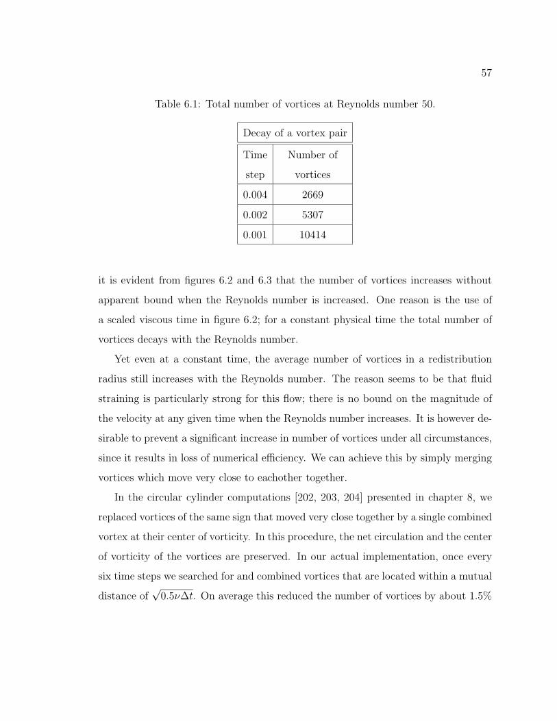
57

Table 6.1: Total number of vortices at Reynolds number 50.

Decay of a vortex pair

Time Number of

step vortices

0.004 2669

0.002 5307

0.001 10414

it is evident from figures 6.2 and 6.3 that the number of vortices increases without

apparent bound when the Reynolds number is increased. One reason is the use of

a scaled viscous time in figure 6.2; for a constant physical time the total number of

vortices decays with the Reynolds number.

Yet even at a constant time, the average number of vortices in a redistribution

radius still increases with the Reynolds number. The reason seems to be that fluid

straining is particularly strong for this flow; there is no bound on the magnitude of

the velocity at any given time when the Reynolds number increases. It is however de-

sirable to prevent a significant increase in number of vortices under all circumstances,

since it results in loss of numerical efficiency. We can achieve this by simply merging

vortices which move very close to eachother together.

In the circular cylinder computations [202, 203, 204] presented in chapter 8, we

replaced vortices of the same sign that moved very close together by a single combined

vortex at their center of vorticity. In this procedure, the net circulation and the center

of vorticity of the vortices are preserved. In our actual implementation, once every

six time steps we searched for and combined vortices that are located within a mutual

distance of√

0.5ν∆t. On average this reduced the number of vortices by about 1.5%

58

each time. Using this procedure, we did not experience a significant increase in scaled

vortex density with Reynolds number.

It should be emphasized that condensing nearby vortices into single vortices is

not the same as the need to regenerate the mesh in particle methods. First, the only

purpose here is merely to increase numerical efficiency, not to maintain accuracy. Our

computation can continue without it, although at lower efficiency. Second, there is

no need to produce a new ordering, or association, of the computational points; there

is no repartitioning of the domain; there is no quadrature rule to update. We simply

give one vortex the combined strength and location, and drop the other vortex from

the further computation.

It is even possible to incorporate this condensation directly into the redistribution

process itself. For a vortex located close to another vortex, we might simply try to find

a solution to the redistribution equations that does not involve the vortex itself. The

vortex then loses all its circulation and can be removed. The redistribution fractions

could be required to be positive as before, or a less restrictive condition might be

imposed to remove even more vortices. In particular, the convergence analysis for

Stokes flow in chapter 5 would not be affected if the fractions were merely bounded

in the l1 norm and the circulation was allowed to grow by a relative amount O(∆t).

More research is needed to settle these points.

Next we discuss the “cut-off” circulation mentioned in subsection 6.2.3.

6.2.5 Cut-off circulation

As mentioned in subsection 6.2.3, the edges of expanding vorticity distributions

are characterized by exponentially small vorticity. Without special care, this would

lead to large amounts of computational vortices of extremely small strengths, severely

affecting the computational efficiency. To avoid this, some minimum or “cut-off”

vortex strength is chosen; below this strength no new vortices are created. To be

precise, in our computations we do not diffuse the vortices if the absolute value of

59

their circulation falls below a chosen cut-off value ǫΓ. For the computations of the

counter-rotating vortex pair of figures 6.1 through 6.3 we set ǫΓ to the machine epsilon.

Figure 6.2 shows that with this cut-off, the growth of the number of vortices is roughly

linear in time. This indicates that the cut-off works well, since for this flow the true

area containing vorticity also grows roughly linear in time. Mesh refinements and

comparisons with other data in sections 7.1 and 7.2 indicate that the computational

accuracy is not affected by the cut-off.

The use of a cut-off circulation amounts to neglecting the exponentially small

vorticity field at the outer edges of the region of vorticity; as a result, the exponentially

small rotational velocity field induced by that small vorticity fields is also neglected.

Before this study, it was generally felt that ignoring such exponentially small

contributions will not affect the solution. For example, for classical boundary layer

problems, the exponentially small velocity above the boundary layer does not have to

be computed accurately. For such computations, it suffices to simply set the vorticity

zero at some position some distance above the boundary layer or to ensure that the

velocity remains finite above the boundary layer through some other means.

However, Van Dommelen & Shen [239] made the surprising discovery that this is

not necessarily true for the long time behaviour of unsteady boundary layers. They

studied the unsteady boundary layer development near stagnation points at the rear

of smooth bodies such as circular cylinders. This problem was earlier investigated

by Proudman & Johnson [177]; however, these authors found that they could not

obtain a unique solution for the long time problem without some ad hoc assumptions

which turned out to be only qualitatively correct. Robins & Howarth [183] took

the expansions of Proudman & Johnson to higher order, but could not remove the

indeterminacy. P. G. Williams [246] further noted that his numerical results did not

seem to agree with the predictions of Robins & Howarth. Van Dommelen & Shen [239]

discovered that the reason was that the long time solution is completely determined by

60

growth of the exponentially small velocities above the boundary layer; these velocities

were ignored in the asymptotic expansions of Proudman & Johnson and Robins &

Howarth. Van Dommelen & Shen [239] noted in their conclusion that this must be

a concern in numerical schemes: setting the exponentially small velocities to zero is

equivalent to eliminating the very information that determines the solution for later

times.

Although subsequent computations for flows such as the impulsively translated

circular cylinder ignored the work of Van Dommelen & Shen [239] on the rear stag-

nation point, (as it did their work on the separation singularity), our computations

in section 8.2 do show a significant dependence of the results on the cut-off value ǫΓ.

Furthermore, we will present indications that other authors have in fact experienced

computational problems because of values of ǫΓ that were too optimistic.

In the next subsection we will discuss how our computation evaluates the vorticity

at arbitrary points.

6.2.6 Evaluation of the vorticity

As was discussed in section 4.1, in the redistribution method the diffusion of

vorticity is achieved by changing the strengths Γni of the vortices. Unlike some other

methods, the continuous vorticity field

ω(~x, t) =∑

i

Γi φδ(~x− ~xi(t)) , (6.10)

is not differentiated or even evaluated during diffusion. The equations 4.8 governing

diffusion are completely independent of the “vortex core shape” φδ in the representa-

tion of the vorticity field above. Thus the vortex core φδ does not appear in the actual

computation. To be precise, while the diffusion process is independent of the vortex

core, the implementation of convection of section 6.1 still requires one. Our choice

(6.2), (6.3) for the core shape φδ has a relatively low second order accuracy [106],

but it is everywhere positive. The reason we chose this function is that unsteady

61

separating flows at large Reynolds numbers involve short scale vorticity features that

can be lost by large core sizes. This makes a small core size desirable regardless of the

order of accuracy of the core. For a small core size, a relatively low order of accuracy

can be sufficient; and other considerations may be more important. In particular,

positive second order cores such as the one we used have the advantage that they

cannot introduce false vorticity of opposite sign.

Another place we use the vortex core is when we need to evaluate pointwise

vorticity values for output purposes. In this case the considerations for the choice of

the most desirable core are somewhat different. For maximum visual smoothness, a

large core is desirable, since a large core gives the greatest reduction in short wave

errors. These short wave errors are further also much more pronounced in the vorticity

field than in the velocity evaluation during convection. On the other hand, there is

much less risk that a larger core would smooth small features, since the actual solution

is now known, and the effect of core size can be determined experimentally without

repeating any of the computation. Further, even if there would be some loss of

information about the shorter wave lengths in the output for the vorticity, this loss

does not affect the further computation. Such considerations suggest the use of a

second core different from the one used for convection to do the output. In fact, there

is no good reason why the two cores would need to be the same. So, for evaluation

of the vorticity, we choose a second core with a high order of accuracy, since these

can be larger for a given accuracy. Thus, for the computations of flows in free space

in sections 7.1 and 7.2, we choose our second smoothing function to be a relatively

large but infinite-order core

φδ(~x) =1

δ2φ

(~x

δ

)

, (6.11)

in which

φ(~x) =1

2π

J1(|~x|)|~x| , (6.12)

62

where J1 is the Bessel function of the first kind of order one. This smoothing function

was first proposed by Leonard [126].

As shown in section 7.2, the results are not very sensitive to the precise choice of

either of our core shapes. In most computations in this thesis, as in [201], a core size

δ of 2.4√ν∆t to 3.5

√ν∆t was used, where ν is the kinematic viscosity and ∆t is the

time step.

Near boundaries, the determination of the pointwise vorticity field runs into diffi-

culties, since the vorticity field beyond the boundary is unknown. In order to compute

the correct vorticity near a boundary, the vorticity field must be extrapolated into

the boundary in some way.

For our computations of flows around circular cylinders of unit radius in chapter

8, we extrapolated the vorticity into the cylinder by mirroring every vortex into the

cylinder to a radial position that is the inverse of the radial position of the original

vortex. Further, we changed the strengths of the thus mirrored vortices so that

a constant vorticity level outside the cylinder would be extrapolated into a constant

vorticity level within the cylinder. It is easily seen that this requires that the strength

of each mirrored vortex is reduced by a factor equal to the radial position of the vortex

to the power four.

Using this procedure, vorticity fields that are about constant near the wall can

be evaluated without difficulty. However, if there are appreciable gradients, they will

affect the evaluation of the vorticity. This is evident in our computations of the flow

about a cylinder in rotational oscillations in figure 8.2. As expected, our procedure

produces a local average of the vorticity near the wall, rather than a pointwise vorticity

value at the wall.

To remove such errors would require that the vorticity field is linearly extrapolated

into the cylinder, rather than as a constant. This would require some additional

coding effort, but does not seem particularly difficult from a fundamental point of

63

view. For a cylinder in steady rotation, figure 8.1 the vorticity flux vanishes at the

wall and the error in our simple procedure is much smaller.

One additional modification needed near solid walls concerns the smoothing func-

tion. The smoothing function (6.11) decays too slowly at large distances to be useful

for flows with solid boundaries; for these flows the vorticity can only be extrapolated

a small distance into the boundary. Instead, for the flows over circular cylinders in

chapter 8 we chose φ to be a fourth-order Gaussian of form [17],

φ(~x) =1

π

(2 e−|~x|2 − 1

2e−2|~x|2

). (6.13)

In these computations a core size δ = 3.5√ν∆t was used.

A final smoothing function was used to evaluate the vorticity in three-dimensional

flows in free space in section 7.3. For two-dimensional flows in free space in sections

7.1 and 7.2, Leonard’s infinite order smoothing function (6.12) above gives excellent

results. In three dimensions, the equivalent infinite order smoothing function is

φ(~x) =1

(2π)3/2

J 3

2

(|~x|)|~x|3/2

, (6.14)

where J 3

2

is the fractional order Bessel function of the first kind of order 32. However,

this function decays too slowly at large distances to be useful: even constant vorticity

fields cannot be represented by it. The reason for the slow decay of the smoothing

function (6.14) is its Fourier transform, which is shown as a dotted line in figure

6.4(a). It is unity for wave number k less than one and vanishes for larger k. The

resulting discontinuity causes the slow decay of the smoothing function itself. To

obtain faster decay, we must smooth the discontinuity. We choose:

φ(k) =1

e2(k2−k−2) + 1, (6.15)

where k is the wave number in the radial direction. This produces an infinite or-

der smoothing function that also decays exponentially at large distance. Since this

64

core cannot readily be evaluated in physical space, we approximated it by a spline

interpolant (figure 6.4b).

To apply the numerical implementation discussed so far to flows over solid walls

we need to address the numerical handling of the boundary condition on solid walls;

we will describe that in the next section.

6.3 Boundary condition

In this section we will describe the numerical implementation of the boundary

condition on a solid impermeable wall (2.5),

~u(~s, t) = ~us(~s, t) , (6.16)

where ~s is any point on the solid wall, ~u is the velocity of the fluid, and ~us is the

prescribed velocity of the solid wall.

The above boundary condition (6.16) is a vectorial condition and it is equivalent

to two conditions, namely, the normal and tangential components of the fluid velocity

on the solid wall must be the same as those of the wall:

Normal condition:

~u(~s, t) · n = ~us(~s, t) · n , (6.17)

Tangential condition:

~u(~s, t) × n = ~us(~s, t) × n , (6.18)

where n is the unit vector normal to the solid wall; the tangential condition (6.18) is

also known as the no-slip condition [14].

65

One possible way of satisfying the normal condition (6.17) is by first evaluating

the velocity induced by the vorticity field according to the free space Biot-Savart law

(2.16). We will denote this velocity by ~uω. Next we add to this an irrotational velocity

~uΦ chosen to satisfy the normal flow boundary condition. This potential flow velocity

can be obtained from a scalar function Φ [14, 129],

~uΦ ≡ ∇Φ (6.19)

∇2Φ = 0 (6.20)

∇Φ(~s, t) · n = (~us(~s, t) − ~uω(~s, t)) · n . (6.21)

In an unbounded domain, the potential flow should also provide the correct velocity

at large distances from the body.

However, in our computations of flows over circular cylinders discussed in section

8.2, we followed a different procedure. In our work, ~uΦ was obtained from the sum of

the potential flow velocity due to uniform translation of the cylinder and the potential

flow velocity due to so called “image vortices” inside the cylinder [156, 245].

The tangential boundary condition is somewhat more complicated. The velocity

field produced by the vorticity and normal boundary condition produces a velocity

~u(~s, t) of the fluid at the wall equal to

~u(~s, t) = ~uω(~s, t) + ~uΦ(~s, t) . (6.22)

The tangential velocity difference (~us(~s, t) − ~u(~s, t)) × n is called the slip velocity

[129].

Assuming that the slip velocity is zero at some given time, it will no longer be so

at the end of the time step after we have convected the vortices and diffused them.

One reason is that it is impossible to satisfy the no-slip boundary condition during

the convection step. Also, since the no-slip boundary condition is on the velocity and

not on the vorticity, there is no simple way to satisfy this boundary condition during

66

our diffusion procedure. Instead, during our diffusion step we satisfy an approximate

zero vorticity flux boundary condition, which is easy to accomplish by “mirroring”

the vortices into image vortices inside the wall.

The erroneous boundary conditions during the time step will produce an additional

“Stokes layer” of typical thickness O(√ν∆t) compared to the solution with the true

no-slip boundary condition.

We remove this erroneous Stokes layer at the end of the time step by adjusting

the vortex strengths near the wall to satisfy no-slip. Of course, the detailed profile

of the Stokes layer is unknown, but since its thickness is of the order of the smallest

scale in our computation, this is not important. Its net vortex strength is known;

since the layer is thin, it equals the slip velocity at the end of the time step.

Note, however, that the evaluation of the slip velocity is a somewhat tricky proce-

dure. The velocity will fluctuate strongly due to local perturbations induced by the

vortices immediately adjacent to the wall. Our solution to this problem is simple:

since the thickness of the Stokes layer is our smallest resolved size, we can to the

accuracy of our computation replace it by a regularly spaced string of vortices along

the wall. The strength of this string of vortices is then constantly updated such that

the no-slip boundary condition remains satisfied. To do so, we simply remove all

vortices in the Stokes layer, evaluate the resulting slip, and add the string of vortices

back in, with a strength given by the found local slip. More precisely, the strength of

each vortex in this string is found by integrating the slip velocity over its segment of

the wall.

In our numerical implementation, we chose a string of vortices at a distance of√

0.5 ν∆t from the wall. Note that if the error in wall velocity would be a constant

during the time step, it would lead to a classical Stokes layer with in a mean diffu-

sion distance 0.96√ν∆t. For the more reasonable assumption that the error in wall

67

velocity increases linearly across the time step, it would produce a Stokes layer with

a mean diffusion distance of 0.57√ν∆t.

This procedure was used earlier by Van Dommelen [237] and Wang [245] in random

walk computations and is quite robust. Suppose that the overall vorticity level in the

boundary layer is too low by a finite fraction, then we would compute a finite slip

velocity. Across the thin strip at the wall represented by the string of vortices, this

would produce a string of very strong vortices which would lead to a very large

vorticity flux into the remaining boundary layer. This flux would quickly restore the

vorticity level in the boundary layer to the correct strength.

Note that this argument does not depend critically on the parameters used, al-

though the vorticity flux out of our string must of course be of the correct general

order of magnitude. Further, in our implementation the actual strengths of the string

vortices have little effect on the rest of the computation since their velocity field is

almost completely canceled by the very close by image vortices within the wall.

Also, stability is enhanced by the fact that we do not just update the strengths

of the vortices, but instead create a new string of vortices after first removing all

vortices from the strip at the wall. This increases stability since short-scale streamwise

fluctuations that might exist in the boundary layer die out across the empty potential

flow strip and have little effect on our numerical determination of the slip velocity.

We chose the spacing of the vortices in the string to be√

6 ν∆t, which is the

same distance at which we place newly added vortices in our redistribution method

(subsection 6.2.3).

The implementation of no-slip condition described above is admittedly a heuristic

approach. However, it is simple to apply and gives accurate results as shown in chapter

8. Our computational results are in excellent agreement with analytical solutions of

Van Dommelen & Shankar (unpublished), and recent higher order (fourth-order in

68

space and time) finite difference solutions of Anderson & Reider [3] and spectral

element solutions of Kruse & Fischer [120].

6.4 Summary

As described in section 6.1, the convection of the vortices can be handled nu-

merically using a mesh-free algorithm. The diffusion of the vortices can now also be

handled in a mesh-free manner using our new method as described in section 6.2. The

simple numerical implementation of the no-slip boundary condition on solid walls was

described in section 6.3. In the following two chapters we will present the results of

the numerical implementations discussed.

CHAPTER 7

COMPUTATION OF FLOWS IN FREE SPACE

In this chapter we apply the vorticity redistribution method to several flows in

free space. We present numerical results for the two-dimensional flow due to the

diffusion of a single point vortex in section 7.1 and due to the diffusion of a pair of

counter-rotating point vortices in section 7.2. In section 7.3 we present results for two

simple Stokes flows in three-dimensional free space: the flow due to a pair of vortex

poles and the flow due to a vortex ring.

7.1 Point vortex

In this section we study the flow due to a two-dimensional point vortex in free

space. We will first present the governing equations of the flow in subsection 7.1.1.

The numerical results to validate the performance of the redistribution method are

presented next in subsection 7.1.2.

7.1.1 Governing equations

The flow studied here is that due to a diffusing point vortex of strength Γ. We

will normalize this problem by means of Γ/2π and an arbitrary characteristic length

ℓ. We take the Reynolds number of the flow correspondingly as Re = Γ/2πν. Thus

normalized, the problem is governed by the nondimensional vorticity equation

ωτ = ωxx + ωyy −Re(uωx + vωy) , (7.1)

where τ is a diffusion time defined as τ = t/Re.

69

70

The initial condition is

ω(x, y, 0) = 2πδ(x, y) , (7.2)

where δ(x, y) is the two-dimensional delta function.

The velocity follows from the Biot-Savart law [14], or equivalently from the stream

function ψ:

∇2ψ = −ω u = ψy v = −ψx . (7.3)

Note that the problem is independent of the length scale ℓ, since the Reynolds

number is. The only relevant length scale is the computational vortex spacing as

compared to the diffusion distance√

4 ν t. Our computation will therefore proceed

from initial stages with no numerical resolution at all to later stages of increasing

resolution. Despite the lack of resolution in the early stages, our computation turns

out to be accurate (see section 9.1 for related theoretical results).

7.1.2 Vorticity field

The chosen problem is a good test case since an exact solution exists: its form is

same as that of a diffusing point heat source governed by the heat equation. Oseen

[122] pointed out that this provides a solution not just to the linear Stokes equations

for Re = 0, but also to the nonlinear Navier-Stokes equations (7.1) through (7.3) for

Re 6= 0. The reason is that the convection terms at the end of (7.1) vanish identically

for this flow: the streamlines are circular and coincide with the direction of constant

vorticity. But, while convection is trivial for the exact solution, it is not for the

discretized solution: the discretization produces noncircular streamlines as well as

other numerical errors.

We will present numerical results for Reynolds numbers of 0, 10, 50 and 100.

Because of data available in literature, we computed the range 0 ≤ τ ≤ 0.3. Note

that the maximum value of τ by itself is of no relevance to this flow since there is

no inherent length scale; the only important parameter is the maximum ratio of τ

71

to the typical nondimensional area per computational point. We used a numerical

time step ∆τ = 0.002 and we also repeated all computations at ∆τ = 0.004 to verify

their accuracy. As explained in subsection 6.2.3, we performed redistribution over

a neighborhood of radius√

12∆τ . Where no solution to the redistribution problem

could be found, we added new vortices at a distance√

6∆τ . We used the vortex

core (6.3) of size δ =√

0.5 ν∆t in integrating the convection processes, and the core

(6.12) of size δ = 2.4√ν∆t to δ = 3.5

√ν∆t to evaluate pointwise vorticity values.

The computations were carried out in 32 bit precision on a VAX4000-300 computer

running VMS V6.0.

Other investigations of similar flows have focussed on the average square radius

of the vortex, r2 =∑

i Γi(x2i + y2

i )/∑

i Γi, which grows as 4τ . The redistribution

scheme reproduces this growth exactly due to (4.10), while in the absence of numerical

errors the vortex blob method preserves it during the convection step (3.18, 3.19).

Indeed figure 7.1 shows excellent agreement between the computed and exact values

of r2, indicating that the solution of the redistribution equations and the numerical

integration of convection are accurate. The relative error is of order 10−6.

According to the exact solution, circulation should be preserved; in our numerical

solutions it was preserved to six digits accuracy. Further, according to the exact

solution the mean vortex position should remain at the origin. In our numerical

results for the Stokes flow, it does so to an accuracy of 10−7. This error increases

to the order of 10−5 for higher Reynolds numbers in agreement with the chosen

truncation error in the fast velocity summation scheme [233]. It is clear from existing

studies such as [78, 79, 155, 182] that such accuracy could not be achieved using the

random walk method with the same number of vortices.

Despite the arbitrary locations of the vortices, it is possible to obtain accurate

pointwise vorticity values. For example, figure 7.2 compares the numerical vorticity

along a horizontal line with the exact solution. A close examination shows that since

72

the infinite-order smoothing function is not entirely positive, it produces very small

negative vorticity at the tail end of the distribution. The maximum errors at τ =0.082

and 0.202 are 0.046 and 0.016 respectively, which amounts to 0.75% and 0.65% of the

maximum vorticity. Results such as those of Fogelson & Dillon [79] show clearly

that the random walk method cannot achieve such pointwise accuracy without an

excessive number of vortices.

Table 7.1 shows the number of vortices and computational times for the fast

summation and redistribution parts of the computation. It should be noted that the

time needed for convection is increased due to subdivision of the convective time-

step: since the flow starts from a concentrated vortex, during the first few time-steps

the vortices rotate rapidly about each other. To limit the corresponding numerical

errors, the early convection time steps were subdivided further. For example, at

Reynolds number 50, the first convection step was subdivided into 50 equal parts.

The subdivision was then decreased inversely proportional to the time-step number.

Since the number of vortices at early times is very small, the additional amount of

work is limited.

As discussed at the end of subsection 6.2.1, the diffusion time may be greatly

reduced for Stokes flow, and most likely also for other Reynolds numbers, by not

solving the redistribution equations from scratch each time-step. As discussed at the

end of subsection 6.2.3, the number of vortices at high Reynolds number may be

reduced by some form of regeneration of the vortex distribution. This was not done

here.

In any case, table 7.1 shows very clearly that the computational time for diffusion

is acceptable even using our simple initial approaches. To put this in perspective,

note that it requires 16 times more computational effort to resolve spatial scales that

are only smaller by a factor 2. In addition, we may note that our method resolves

73

Table 7.1: Computational times for a point vortex at τ = 0.202 and ∆τ = 0.002.

Decay of a point vortex

Reynolds Number of Convection Diffusion

number vortices CPU secs CPU secs

0 2482 0 2363

10 2863 1723 2724

50 3896 3320 4216

smaller scales than competing vortex methods for the same number of vortices (see

section 9.1).

7.2 Counter-rotating vortex pair

In this section we study the flow due to two counter-rotating vortices in free

space. For this flow, convection is nontrivial even for the exact solution. We will first

present the governing equations of the flow in subsection 7.2.1. The numerical results

to validate the performance of the redistribution method are presented in subsection

7.2.2; we will compare the computed vorticity at small times with analytical solutions

Van Dommelen & Shankar [230]. We compare the long time numerical results with

analytical predictions in subsection 7.2.3.

7.2.1 Governing equations

The flow studied here starts from two counter-rotating point vortices. We use the

same nondimensionalization as for a single point vortex in subsection 7.1.1, but in

addition we now chose the characteristic length ℓ as the distance between the initial

74

point vortices. This leads again to the vorticity diffusion equation

ωτ = ωxx + ωyy −Re(uωx + vωy) . (7.4)

However, the initial condition is now:

ω(x, y, 0) = 2πδ(x− 12, y) − 2πδ(x+ 1

2, y) . (7.5)

This vortex system will drift in the direction normal to the line connecting the vortices.

Using our normalizations, the initial drift velocity will be unity (which explains our

choice of normalizations). The Reynolds number Re = Γ/2πν can therefore also be

considered to be based on the initial drift velocity and the vortex spacing.

The velocity again follows from the Biot-Savart law [14], or equivalently from the

streamfunction ψ:

∇2ψ = −ω u = ψy v = −ψx . (7.6)


The considered flow is a more severe test case than the one of section 7.1 since

convection is not trivial even for the exact solution. It also involves mutual cancel-

lation of negative and positive vorticity, which random walk computations do not

handle very well [235].

For the Stokes flow Re = 0, the exact solution exists: it is simply a superposi-

tion of two single diffusing vortices. Figure 7.3 shows the vorticity distribution along

the line connecting the initial point vortices. There is excellent agreement between

the exact solution and the computed vorticity. This is also evident from the com-

puted vorticity lines figure 7.4. As demonstrated by Van Dommelen [235], a standard

random walk approach would experience considerable difficulty with this flow since

vanishing vorticity is there approximated by roughly equal amounts of negative and

positive vortices of the initial strength.

75

Unfortunately, for nonzero Reynolds number no exact analytical solution is avail-

able to show how well the nontrivial convection effects are represented. Instead, we

use the second order expansion derived by Van Dommelen & Shankar [230] which

is valid for sufficiently small times. To obtain high resolution for small times, we

performed the computations in this section at ∆τ = 0.00025.

Figure 7.5 shows vorticity contours for Reynolds number Re = 50 at two early

times. The dashed curves in this graph represent the first order solution given by a

simple superposition of single vortex solutions, while the solid curves include the next

order in the small time expansion developed by Van Dommelen & Shankar [230]. The

difference between the curves represents nontrivial convection effects. Since the two

curves are close together in figure 7.5(a), we expect the small time approximations

to be very accurate; hence the exact solution should be close to the solid curve.

Our computations do reproduce this expected curve closely. We consider this to be

excellent performance of both the small time expansion and our numerical scheme

(especially for a vortex method with an arbitrary point distribution). Note that the

time is no longer truly small: the vortices have already expanded to a size comparable

to their distance!

At still later times, the small time expansion is probably no longer accurate, since

it is based on the approximation that the size of the vortices is small compared to

their distance. The inaccuracy is reflected in sizeable differences between the solid

and dashed curves in figure 7.5(b). While the exact solution is now no longer certain,

we still believe that it is accurately represented by our numerical solution. One reason

is that the computed solution is closer to the solid curve; secondly, we expect the next

higher-order term in the small time expansion to have three periods along a contour,

which seems to agree with the number of curve crossings in figure 7.5. Table 7.2 shows

the number of vortices and computational times at τ = 0.202. The computations were

carried out in 32 bit precision on a VAX4000-300 computer running VMS V6.0.

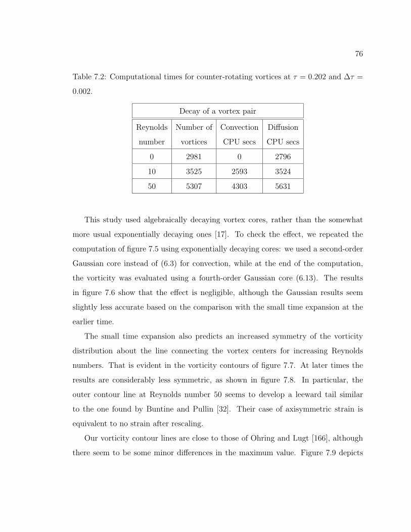
76

Table 7.2: Computational times for counter-rotating vortices at τ = 0.202 and ∆τ =

0.002.

Decay of a vortex pair

Reynolds Number of Convection Diffusion

number vortices CPU secs CPU secs

0 2981 0 2796

10 3525 2593 3524

50 5307 4303 5631

This study used algebraically decaying vortex cores, rather than the somewhat

more usual exponentially decaying ones [17]. To check the effect, we repeated the

computation of figure 7.5 using exponentially decaying cores: we used a second-order

Gaussian core instead of (6.3) for convection, while at the end of the computation,

the vorticity was evaluated using a fourth-order Gaussian core (6.13). The results

in figure 7.6 show that the effect is negligible, although the Gaussian results seem

slightly less accurate based on the comparison with the small time expansion at the

earlier time.

The small time expansion also predicts an increased symmetry of the vorticity

distribution about the line connecting the vortex centers for increasing Reynolds

numbers. That is evident in the vorticity contours of figure 7.7. At later times the

results are considerably less symmetric, as shown in figure 7.8. In particular, the

outer contour line at Reynolds number 50 seems to develop a leeward tail similar

to the one found by Buntine and Pullin [32]. Their case of axisymmetric strain is

equivalent to no strain after rescaling.

Our vorticity contour lines are close to those of Ohring and Lugt [166], although

there seem to be some minor differences in the maximum value. Figure 7.9 depicts

77

our results for the maximum vorticity as a function of time, along with the Oseen

(small time or single vortex) and Stokes (large time) values. Our results follow the

Stokes curve closely regardless of Reynolds number; this agrees with the results of Lo

and Ting [132] for a similar flow.

Figure 7.10 shows the distance of the vorticity maximum away from the symmetry

line for Reynolds numbers 0, 10, 50, and 100. While a maximum is hard to locate

in a vortex method with an arbitrary distribution of vortices, our results agree well

with the exact Stokes solution (Re = 0) and with the results of Ohring and Lugt. In

particular we agree with the conclusion of Ohring and Lugt that the maximum moves

away from the symmetry plane at all times.

Figure 7.11 shows the decay of the circulation in a half plane with time. We find

no dramatic change in circulation with Reynolds number, although the circulation at

higher Reynolds numbers decays somewhat more slowly. Our results at zero Reynolds

number are almost identical to the exact Stokes solution. These results agree with

those of Ohring and Lugt [166]. They also agree with the results of Buntine and

Pullin [32] for a smoothed initial condition. Their results at Reynolds numbers 40

and 160 are indistinguishable, similar to our results at 50 and 100. Our curve for

Reynolds number 100 ends up between those for 10 and 50.

For this flow, the velocity increases without bound when the Reynolds number

increases, especially for small times. This leads to almost singular convection terms

at high Reynolds numbers. Yet, our numerical results show that the redistribution

method captures such strong convection effects very accurately. Further evidence of

the accuracy and reliability of our method, including longer times, will be presented

in the next section in which we discuss the propagation or drift velocity of the vortex

pair.

78

7.2.3 Drift velocity

In the previous subsection we verified our numerical solution against a small time

prediction for the vorticity field. In this section we will verify the numerical results for

longer times against analytical predictions. In particular, we will examine the path

and the velocity of the vortex pair. Those are important quantities in many practical

applications. For example, a vortex pair provides a simple model for investigating the

trailing vortices behind the wings of large aircrafts [131, 167, 223, 253]; these vortices

persist over long distances and are hazardous for smaller aircrafts in the vicinity of

these vortices. Hence, it is important to know where the vortices end up. As an

other example, the trailing vortices from a ship are also modeled by a vortex pair

[141, 194, 226]; and the interactions of these vortices with the free surface of the sea

produce characteristic signatures in radar images.

The drift velocity of two counter-rotating point vortices in an inviscid (to be

precise, for Re = ∞ and t = τ Re finite) fluid is simple: the vortex pair drifts in the

direction of the symmetry line (here the y-axis) at constant speed [230]. Further, in

the inviscid case the positions of the vortices are simple to identify since the point

vortices remain point vortices

However, in a viscous fluid the vortex pair diffuses, and changes shape and speed

as it drifts. Hence, before we can compare the numerical results, we need to define first

what point will be taken as the “position” of the vortex pair. Different authors have

used different points to measure the position; the time derivatives of these different

points imply different drift velocities. We will first review some of these definitions.

Since the flow is symmetric about the y-axis, we will focus on the flow in one half

plane bounded by this symmetry line. One way to define a position of the vortex in

the chosen half plane is to average over the vorticity:

yc =

∫ ∫y ω dx dy

∫ ∫ω dx dy

, (7.7)

79

where the integration is over the half plane. We will define the drift velocity obtained

as the time derivative of yc to be the vortex center velocity vc. Instead, Saffman [191]

defines the vortex position to be

yg =

∫ ∫x y ω dx dy

∫ ∫xω dx dy

. (7.8)

We will denote the time derivative of yg to be the velocity vg. Next, Ohring and Lugt

[166] define the vortex position to be the location of the vorticity extremum, giving

still a different velocity. In addition to these drift velocities, we can define an average

velocity v in the direction of propagation as

v =

∫ ∫v ω dx dy

∫ ∫ω dx dy

, (7.9)

where v is the component of the velocity field in the direction of propagation.

The limiting behaviors of the drift velocities defined above are investigated by

Van Dommelen & Shankar [230] for small times, for small Reynolds numbers, and

for large times using asymptotic expansions. In the following paragraphs, we com-

pare the numerical results obtained using the vorticity redistribution method with

the analytical solutions obtained there. The Reynolds number in the computation

ranges from 0 to 100 based on the initial drift velocity. The computational results

presented in this subsection were obtained at a diffusion time step ∆τ = 0.002 and

were repeated at 0.004 to verify their accuracy. At the highest Reynolds number

Re = 100, we halved the time step again (to 0.001) to eliminate some unsightly, but

inconsequential wiggles. In addition, for shorter times, computations were conducted

at a still smaller time step (∆τ = 0.00025) to verify very small perturbations in the

small time analytical solution.

Figure 7.12 shows analytical and semi-analytical results of Van Dommelen &

Shankar [230] for the computed velocities v, vc and vg for Reynolds number Re = 0,

as well as the small and large time expansions for that case. At small times, the

average velocity v and the vortex center velocity vc remain exponentially close to the

80

unit inviscid drift velocity. On the other hand, the velocity vg decreases proportional

to the diffusion time τ . Figure 7.12 also shows that the asymptotic values for the

average velocity v and velocity vg for large times are still quite inaccurate at the

maximum times presented here. The computed vortex center velocity vc tends to the

computed velocity vg for large times; but the computed average velocity v remains

larger than these two velocities by about 10% [230].

As shown in figures 7.13 and 7.14, our computed results at a very fine time step

(∆τ = 0.00025) correctly follow the analytical predictions for small times [230]. Note

that this indicates excellent performance of the numerical method: the graph verifies

very small deviations from the inviscid drift velocity. Furthermore, the velocity is

almost singular at those times. In figures 7.13 and 7.14, the exact Stokes solution for

Re = 0, has also been shown. At larger times all computed curves should approach

the Stokes curve since the decay of the circulations of the vortices reduces the effects

of convection. This is consistent with our numerical results.

Figures 7.15, 7.16, and 7.17 show the computed average velocity v, vortex center

velocity vc and the velocity vg for Reynolds numbers 10, 50, and 100. No dramatic

changes from Stokes flow are observed for the studied Reynolds numbers. Moreover,

the different computed velocities have an interesting tendency to approach each other

when the Reynolds number increases. For example, figure 7.18 compares these veloc-

ities at Reynolds number 100. Theoretical reasons why this would be so can be found

in Van Dommelen & Shankar [230].

7.2.4 Summary

We investigated the flow of the counter-rotating vortex pair for Reynolds numbers

based on the drift velocity ranging from 0 to 100 based on the drift velocity. Our com-

putations reproduced the small time analytical results of Van Dommelen & Shankar

[230] accurately. For large times, and for large Reynolds numbers the behavior of the

computed drift velocities agree also well with analytical predictions. In general, our

81

numerical results agree also with those of Ohring and Lugt [166], Lo and Ting [132],

and Buntine and Pullin [32], even though the latter two studies used a smooth initial

condition. This provides additional support for the numerical results presented in

this subsection. In the next section we apply the vorticity redistribution method to

three-dimensional Stokes flows in free space.

7.3 Three-dimensional Stokes flows

To show that the redistribution method works equally well in three dimensions,

we consider two linear problems [202]: diffusion of a pair of opposite vortex poles and

the Stokes flow (Re = 0) due to a vortex ring in free space.

Figure 7.19a shows the vorticity distribution of the vortex pair along the line

connecting the vortices. Figure 7.19b shows the isovorticity contours in the right half

of the plane containing the vortices. The solid lines are exact solutions and the dots

are computed solutions; the solutions are in very good agreement. Our computations

show that the circular symmetries in the solution are reproduced very well, even

though the symmetries are not explicitly enforced.

Figure 7.20 shows the vorticity field due to the diffusion of a vortex ring at two

different times. It is seen that the mean thickness of the ring expands correctly as

expected and also preserves the circular symmetry very well.

Hence, the results presented in this chapter show that the vorticity redistribution

method can handle flows in free space accurately. In the next chapter we will apply

the vorticity redistribution method to two-dimensional flows over solid walls.

CHAPTER 8

COMPUTATION OF FLOWS OVER SOLID WALLS

In this chapter we apply the vorticity redistribution method to flows over solid

walls. We first compute axisymmetric flows over impulsively rotated circular cylinders

in section 8.1. Next, we compute the more difficult case of an impulsively translated

circular cylinder in section 8.2. Finally, we investigate the interaction of vortices with

a solid wall is in section 8.3.

8.1 Impulsively rotated cylinder

To check the numerical implementation of the boundary condition described in

section 6.3, we first compute two axisymmetric flows. For these two flows there exist

exact solutions or easily computed finite difference solutions.

The first flow we consider is the Stokes flow (Re = 0) over a circular cylinder

impulsively set into an uniform rotation about its axis. The boundary condition on

the cylinder surface is the no-slip condition (2.5); the vorticity vanishes far away from

the cylinder surface. Figure 8.1 shows that the computed vorticity distributions agree

well with the finite difference solutions.

The second flow we consider is the Stokes flow around a circular cylinder set into

periodic rotational oscillations about its axis. This periodic motion is taken to be

cos(τ); where τ is the viscous time t/Re. The boundary condition on the cylinder

surface is the no-slip condition (2.5), while the vorticity vanishes far away from the

cylinder surface. Figure 8.2 shows the vorticity field along a radial line at different

82

83

times during the first time period of oscillation. The numbers 1 to 8 close to the curves

indicate the relative phase of the oscillation; they are 1/8 of the time period apart.

Initially a Stokes layer develops on the cylinder surface. For large times, the flow

becomes periodic due to the periodicity of the boundary condition; our computation

shows that the flow becomes periodic by the end of one time period of oscillation.

The exact periodic solution derived by McLachlan [151] and Winny [248] was used

to check the periodic solutions computed using the finite difference method. The

redistribution solution clearly follows the transient solution computed using finite

differences, and reaches the periodic solution.

It may be noted, however, that the vorticity values on the cylinder surface show

deviations from the finite difference solution. These deviations are not due to the

vorticity redistribution method itself, but arise from evaluating the vorticity using

smoothing functions as discussed in subsection 6.2.6. In fact, figure 8.3 shows that

the total circulation computed by the vorticity redistribution method is in excellent

agreement with the finite difference solution. This must mean that the deviations in

figure 8.2 are only artificial. They can be removed by a more elaborate evaluation

procedure near the wall (subsection 6.2.6). The vorticity distributions in the above

two flows are axisymmetric and our computations reproduced that symmetry very

well even though it was not explicitly enforced.

The excellent agreement of our two-dimensional redistribution results with the

effectively exact one-dimensional finite difference solution provides strong support for

the numerical implementation of the boundary conditions discussed in section 6.3.

However, for these two-dimensional axisymmetric flows, the convection term in the

vorticity equation vanishes identically. To test our method also for flows in which

convection is not trivial, we compute the flow over an impulsively translated circular

cylinder in the next section.

84

8.2 Impulsively translated cylinder

In this section we compute the flow over a cylinder impulsively set into motion

with a constant speed U∞ in the direction perpendicular to its axis. The reason for

choosing this test problem is that for this flow a large number of experimental and

computational results are available to check our computations. We compute the flow

in the reference frame in which the cylinder is stationary and the fluid is streaming

past the cylinder from left to right with speed U∞. The time is nondimensionalized

by U∞ and the radius of the cylinder a. The Reynolds number is Re = 2U∞a/ν,

where ν is the kinematic viscosity of the fluid. The computational results in this

section are presented for the range of Reynolds numbers from 550 to 40,000. All

the computations in this section were performed in 64 bit precision on IBM RISC

System/6000 and single-node SP-2 computers.

We will establish the accuracy of our computed results by comparing them to

experimental, analytical, and recent high-resolution computational results. But first

a review of the more recent computations is presented in subsection 8.2.1. Then, we

check our results for the streamlines in subsection 8.2.2, our velocity fields in subsec-

tion 8.2.3, our vorticity fields in subsection 8.2.4, and our drag forces in subsection

8.2.5. The effect of cut-off circulation parameter (subsection 6.2.5) proves to be very

important and is discussed in subsection 8.2.6. The comparison of our results with

the theory of unsteady boundary layer separation is given in subsection 8.2.7. The

theoretical predictions for the drag force is given in subsection 8.2.8. We compare our

results with the results obtained from other numerical methods in subsection 8.2.9.

8.2.1 Review of previous computations

In this section, we review the numerical schemes used by recent high-resolution

computations; such as those of Anderson & Reider [3], Kruse & Fischer [120],

Koumoutsakos & Leonard [117], and Wu, Wu, Ma, & Wu [249], among others. A

85

review of earlier computations has been given by, for example, Lecointe & Piquet

[123].

Anderson & Reider [3] use a finite difference scheme to compute the flow at

Reynolds numbers Re = 1, 000, 3,000 and 9,500. The vorticity equation and the

Poisson equation for streamfunction are used. Their scheme is fourth-order accurate

in space and time. A fourth-order Runge-Kutta scheme is used for time stepping.

To maintain fourth-order convergence in time a smoothed initial vorticity distribu-

tion is used. Anderson [7] obtains the boundary condition for the vorticity from an

integro-differential equation, which he derives by enforcing both the no-slip condition

and its time derivative. At the outer boundary of the domain, the convection term in

the vorticity equation is discretized using upwind differencing; the diffusion term is

discretized using zero vorticity flux across the boundary. The streamfunction equa-

tion is solved using the domain decomposition method of Anderson [8] for accurate

handling of the velocity boundary condition at large distances away from the cylinder

surface. At the interface of the domains, continuity of the velocity is enforced by an

iterative procedure. For the computation of the flow over the cylinder at Re = 9, 500,

the interface is a circle of radius 1.5 times that of the cylinder and it divides the flow

domain into two annular regions. A 2048 × 256 mesh which is uniformly spaced in

circumferential and radial directions respectively, is used in the inner annular region;

the outer annular region is handled analytically using solutions of the Laplace equa-

tion. They present data for streamlines, isovorticity contours, drag coefficient, surface

pressure, and surface vorticity.

Wu, Wu, Ma & Wu [249] use a finite difference scheme to compute the flow at

Reynolds number Re = 9, 500. The vorticity equation and the Poisson equation for

the stream function are used. A viscous splitting of the vorticity equation is employed.

For the convection of vorticity, the second-order upwind differencing scheme proposed

by B. P. Leonard [127] and the second-order TVD Runge-Kutta time stepping scheme

86

proposed by Shu & Osher [209] are used. For diffusion, the Peaceman-Rachford ADI

factorization with central difference spatial discretization and Crank-Nicholson time

discretization is used. For the boundary condition for the vorticity on the cylinder

surface, the vorticity flux obtained from the momentum equation equation in the

circumferential direction is used. The pressure gradient term in that momentum

equation is found by iteration. The streamfunction at the outer boundary of the

computational domain is obtained from the potential flow velocity due to the transla-

tion of the cylinder; they find that this simplified implementation requires the outer

boundary to be located as far away as possible from the cylinder surface to obtain

accurate results. In fact, their computed radial velocity along the rear symmetry

axis and the drag coefficient are significantly different depending on how far away

the outer boundary is located. In the Re = 9, 500 computational results used for

comparison in the following sections, the outer boundary is a circle of radius 20 times

that of the cylinder. The computational grid consists of 512× 900 mesh points which

are uniformly spaced in the circumferential and exponentially stretched in the radial

directions respectively; and the time step ∆t = 0.0025. They present computational

data for streamlines, radial velocity along the rear symmetry axis, drag coefficient,

slip velocity, and surface vorticity.

Hakizumwami [105] uses a finite difference method to compute the flow at Re =

3, 000 and 9,500; flow symmetry is assumed. The vorticity equation and the Poisson

equation for the streamfunction are used. The vorticity equation is discretized using

a second order central difference scheme. For time stepping, the second order Adam-

Bashforth scheme is used for Re = 3, 000 and the fourth order Runge-Kutta scheme

for Re = 9, 500. A Fourier transform is applied in the tangential direction for the

Poisson equation and the resulting equations are discretized using a second order

central difference scheme. A boundary condition for the vorticity on the surface is

obtained, to second order accuracy, using the streamfunction equation and the no-slip

87

condition. At the outer boundary of the computational domain, the vorticity is set

to zero and the velocity is taken to be the potential flow due to uniform translation

of the cylinder. The grid consists of 120 × 128 mesh points for the Re = 3, 000

and 300 × 128 for the Re = 9, 500; the mesh points are uniformly spaced in the

circumferential direction and exponentially stretched in the radial direction. The

outer boundary is a circle of radius 5 times that of the cylinder. The time step

∆t = 0.01. The computational data for streamlines, radial velocity along the rear

symmetry axis, and surface vorticity are presented.

Loc [133] uses a finite difference scheme to compute the flow at Reynolds numbers

Re = 300, 550 and 1,000; flow symmetry is assumed. The vorticity equation and the

Poisson equation for the streamfunction are used. The vorticity equation is discretized

using a second order accurate scheme. The Poisson equation is discretized using a

compact fourth order accurate scheme. The boundary condition for vorticity on the

surface is obtained to second order accuracy using the streamfunction and the no-slip

condition. At the outer boundary of the computational domain, the vorticity is set

to zero and the velocity was taken to be the potential flow due to uniform translation

of the cylinder. The grid consists of 41 × 41 mesh points for Re = 300, 61 × 61

mesh points for Re = 550 and 81 × 41 mesh points for Re = 1, 000; the mesh points

are uniformly spaced in the circumferential direction and exponentially stretched in

the radially direction. The time step ∆t is 0.05 for Re = 300, 0.033 for Re = 550

and 0.025 for Re = 1, 000. The outer boundary is a circle of radius 20 times that of

the cylinder. The computational data for streamlines, radial velocity along the rear

symmetry axis, drag coefficient, and surface vorticity are presented.

Loc & Bouard [134] use the finite difference scheme of Loc [133] to compute the

flow at Re = 3, 000 and Re = 9, 500. The boundary condition for the vorticity on

the surface is obtained, to second or third order accuracy, using the streamfunction

equation and the no-slip condition. At the outer boundary of the computational

88

domain, a simplified vorticity equation is used. The grid consists of 141 × 101 mesh

points for Re = 3, 000, and 301×101 mesh points for Re = 9, 500; the mesh points are

uniformly spaced in the circumferential direction and exponentially stretched in the

radially direction. A time step ∆t = 0.02 is used. The outer boundary is a circle of

radius 5 times that of the cylinder. They present computational data for streamlines,

radial velocity along the rear symmetry axis, wake length, and surface vorticity.

Kruse & Fischer use a spectral element method to solve the Navier-Stokes equa-

tions in terms of velocity and pressure. The computational grid consists of 6112

spectral elements. There are 10 nodes along each dimension in every element. They

assume flow symmetry in their computation. For their computations at Re = 9, 500,

the outer boundary is a circle of radius 20 times that of the cylinder.

Chang & Chern [40] use a hybrid vortex method to compute the flow at Reynolds

numbers Re = 300, 550, 1,000, 3,000, 9,500, 20,000, 105 and 106. The vorticity

equation and the Poisson equation for streamfunction are used. A viscous splitting

of the vorticity equation is employed. In this hybrid vortex method, a mesh is used

to solve both the streamfunction equation and the diffusion equation arising from

the viscous splitting. The vortex-in-cell scheme proposed by Christiansen [56] is

used to obtain the vorticity at the mesh points from the circulation of the vortices.

The streamfunction at the outer boundary of the computational domain is obtained

by assuming the flow to be uniform there. The vorticity on the cylinder surface is

obtained by applying the streamfunction equation on the boundary together with

the no-slip condition. For most of their computations, the mesh has 128× 200 points

that are uniformly spaced in the circumferential direction and exponentially stretched

in the radial direction. The outer boundary is a circle of radius 25 times that of

the cylinder. The time step ∆t = 0.02. They presented computational data for

streamlines, closed wake (recirculation region) size parameters, “separation” point

(defined as the position where the streamline leaves the cylinder surface, not true

89

separation), radial velocity along the rear symmetry axis, drag coefficient, surface

pressure, and surface vorticity.

Koumoutsakos & Leonard [117] used a vortex method to compute the flow at

Reynolds numbers Re = 40, 550, 1,000, 3,000 and 9,500. No flow symmetry was

assumed. A viscous splitting of the vorticity equation was used (compare subsection

3.2). The velocity field is computed from the circulation of the vortices or “particles”

using a fast scheme based on that of Greengard and Rokhlin [97]. A second-order

Adam-Bashforth time stepping is used to convect the particles. The diffusion is

performed using the Particle Strength Exchange scheme discussed in subsection 1.3.3.

Koumoutsakos, Leonard & Pepin [118] handle the no-slip boundary condition using a

vortex sheet on the cylinder surface; the vortex sheet is allowed to diffuse, leading to

a vorticity flux that modifies the strength of the particles near the cylinder surface. In

the computations, the uniformity of the particle distribution is periodically restored

by remeshing every few time steps. For Re = 9, 500, a time step ∆t = 0.01 is used.

For this computation the number of particles was about 350,000 at time t = 3.00.

They presented computational data for streamlines, vorticity field, circulation, drag

coefficient, position of zero wall shear, surface vorticity, and surface vorticity flux.

Earlier, Pepin [170] also used the Particle Strength Exchange scheme to compute

the flow at Re = 550, 3,000 and 9,500; he assumed flow symmetry. He used the same

fast velocity summation and time discretization as Koumoutsakos & Leonard [117].

For Re = 550 a time step ∆t = 0.03 was used; the number of particles at t = 6.0

was about 50,000. For Re = 3, 000 a time step ∆t = 0.0275 was used; the number

of particles at t = 5.0 was about 76,000. For Re = 9, 500 a time step ∆t = 0.018

was used; the number of particles at t = 3.25 was about 80,000. The remeshing

was performed typically once every six time steps. He presented computational data

for streamlines, closed wake (recirculation region) size parameters, radial velocity

along the rear symmetry axis, vorticity field, drag coefficient, and “separation point”

90

(defined as the position where the streamline leaves the cylinder surface, not true

separation).

Cheer [42] uses the random walk method to simulate the flow at Reynolds numbers

Re = 3, 000, and 9,500. She uses about 900 sheet vortices and vortex blobs; flow

symmetry is imposed by reflecting the vortex elements about the symmetry line. An

Euler time stepping scheme is used and the size of the time step is ∆t = 0.03. For

both the Reynolds numbers, she presents computational data for streamlines, closed

wake (recirculation region) size parameters, radial velocity along the rear symmetry

axis, and “separation point” (defined as the position where the streamline leaves the

cylinder surface, not true separation).

Smith & Stansby [215] use the random walk to compute the flow for Reynolds

numbers Re = 250, 1,000, 10,000, and 105. For convection of the vortices they use

Christiansen’s [56] vortex-in-cell method. The mesh consists of 129 × 200 points

uniformly spaced in the circumferential direction and exponentially stretched in the

radial direction. The outer boundary is a circle of radius 25 times that of the cylinder.

The time step ∆t = 0.02. At each time step, one to six new vortices are created

from each mesh point on the cylinder surface. They present computational data for

streamlines, radial velocity along the rear symmetry axis, drag coefficient, “separation

point” (defined as the position where the streamline leaves the cylinder surface, not

true separation), surface pressure, and surface vorticity.

Van Dommelen [231, 237] uses a random walk method to compute the flow at

Reynolds number Re = 550 and 10,000. The velocity of the vortices are computed

using the fast algorithm of Van Dommelen & Rundensteiner [233]. A second order

Runge-Kutta method (Heun’s method) is used for time stepping. A time step ∆t =

0.025 is used. There are about 7,500 vortices at t = 6.00 for Re = 550 and 25,000

vortices for Re = 10, 000 at t = 3.00.

91

8.2.2 Streamlines

In this subsection we show that our computed streamlines do indeed predict the

flow features observed in the experimental results very accurately.

Computed streamlines are shown in figures 8.4, 8.6 and 8.8 for Re = 550, 3,000,

and 9,500 respectively. Note that the fluid comes from the left of the cylinder. The

characteristic feature is the presence of a large recirculating flow region of closed

streamlines behind the cylinder. The streamwise length of this recirculating region,

also known as the wake length [29], grows in time. The wake length at any fixed time

is smaller for increasing Reynolds number.

A comparison of our computed streamlines with those obtained in the experiment

of Bouard & Coutanceau [29] is shown in figures 8.5, 8.7, and 8.8 for Re = 550, 3,000,

and 9,500 respectively. Our streamlines in the large recirculating flow region behind

the cylinder are in good visual agreement with those of the experiment. In addition

to this large recirculating flow region, a number of smaller recirculating flow regions

along the rear half of the cylinder surface seen in the experiment are also observed

in our computations. As shown by Lecointe & Piquet [123], some of the earlier finite

difference computations were not able to reproduce these smaller recirculating flow

regions.

For completeness, we now give the parameters of our figures 8.4 through 8.8. Using

the usual left-handed x, y coordinate system with origin at the center of the cylinder,

the figure dimensions and streamline contour values are as follows: in figure 8.4 for

Re = 550 and figure 8.6 for Re = 3, 000, x has the range [-1.5,3.0] and y has the

range [-1.4,1.4]; in both these figures, the streamline contour values are 0, ± {0.001,

0.0025, 0.005, 0.01, 0.03, 0.05, 0.07, 0.1, 0.15, 0.2, 0.25, 0.3, 0.35, 0.4, 0.45, 0.5, 0.55,

0.6, 0.65, 0.7, 0.75, 0.8, 0.875, 0.95, 1.025, 1.10, 1.175, and 1.25 }. In figure 8.5 for

Re = 550, x has the range [-0.54,3.75], y has the range [-1.63,1.63], and the streamline

values are same as above. In figures 8.7 for Re = 3, 000, x has the range [-0.16,3.10],

92

y has the range [-1.26,1.26], and the streamline values are same as above. In figure

8.8 for Re = 9, 500, x has the range [-0.25,1.75] and y has the range [-1.05,1.05]; the

streamline values are 0, ±{0.001, 0.003, 0.005, 0.007, 0.01, 0.015, 0.027, 0.04, 0.06,

0.08, 0.1, 0.125, 0.15, 0.18, 0.21, 0.24, 0.27, 0.3, 0.35, 0.4, 0.45, 0.5, 0.55, 0.6, 0.65,

and 0.7 }.In view of the fact that an impulsive start cannot be exactly reproduced experi-

mentally, the agreement between our computation and the experimental data for the

streamlines is excellent. However, many other computations, [40, 117, 134] for exam-

ple, have also shown such good visual agreement between their computed streamline

patterns and those of the experiments. A much stronger test is a comparison of higher

order derivatives of the streamfunction, such as the velocity and vorticity fields, and

the drag force on the cylinder for example. In the next subsection we compare our

computed velocity field with those obtained from both experiments as well as other

computations.

8.2.3 Velocity field

In this subsection we show that our computed velocity field is in excellent agree-

ment with other data such as with the boundary layer computations of Van Dommelen

& Shankar (unpublished) and agrees with other recent high resolution numerical com-

putations by Anderson & Reider [3], Kruse & Fischer [120], and Wu, Wu, Ma, & Wu

[249], as well as experimental data.

For Re = 550, we compare our computed velocity with the experimental results of

Bouard & Coutanceau [29] in figure 8.9. There is very good qualitative agreement but

the wake seems somewhat too thick. We conjecture that slight unsteadiness might add

a bit of eddy viscosity in the experiments. In any case, the computations of Pepin

[170] and Loc [133] in figure 8.10 agree well with our values for the wake length,

instead of with the experiments. There are still some slight differences between those

computations and between those computations and ours. Based on our results for

93

Re = 9, 500 in figure 8.15, discussed later, for which much more reference material is

available, we conjecture that our computations at Re = 550 are the most accurate,

followed by Pepin and then Loc. This is consistent with the fact that the data of

Pepin at Re = 550 are closer to ours than those of Loc.

For Re = 3, 000, we compare our computed velocity with that obtained in exper-

iments of Loc & Bouard [134]. Despite the higher Reynolds number, which tends to

enhance instabilities, the experimental results agree quite well with our data. Again

the experiments show a larger wake size than is supported by our computation. Six

other computations [40, 42, 105, 134, 170, 215] are shown in figure 8.12. Most support

our values for the wake length instead of the experimental ones. A notable excep-

tion is the computation of Loc & Bouard themselves. Again we conjecture that our

computation is more accurate than the other six, with Pepin [170] and Hakizumwami

[105] next. This is again consistent with the data for Re = 9, 500 in figure 8.15.

For Re = 9, 500, better comparisons are possible since there is much more data

available. Further, this flow is more difficult to compute, so that the errors in the

various computations show up more clearly. Also, for this high Reynolds numbers, at

early times the boundary layer is sufficiently thin that the boundary layer approxi-

mation can be used. This is shown in figure 8.13, where both the standard boundary

layer solution as well as second order theory are plotted at time t = 0.5 (unpublished

data of Van Dommelen & Shankar). It may be recalled that in boundary layer the-

ory the velocity is expanded in powers of 1/√Re; standard boundary layer theory

retains only the first term in the expansion (the zeroth power of 1/√Re), while the

second-order boundary layer theory retains the first two terms in the expansion (up

to the first power of 1/√Re). The small difference between the two results shows

that the boundary layer approximation is still applicable. Since the boundary layer

approximation is considerably more straightforward than a Navier-Stokes scheme, fig-

ure 8.13 may be the closest to nontrivial “hard” data that is available for this flow. It

94

is therefore gratifying that our computation produces the most accurate second order

theory closely.

Figure 8.14 compares the computed radial velocity with that obtained in the

experiments of Loc & Bouard [134]. Again the experimental data are in good quali-

tative agreement, but with a somewhat thicker wake than can be supported by our

computations or by most others in figure 8.15.

In figure 8.15, we compare our computed velocity with those of other computa-

tions. All those eight recent computations agree well on the general evolution of the

velocity profile. However, the best agreement occurs between the results of Anderson

& Reider [3], Kruse & Fischer [120], Wu, Wu, Ma, & Wu [249], and our results. This

provides a strong verification of our data. This is further supported by the fact that

the computations we agree with have plenty of resolution: both the mesh based com-

putations use large amounts of mesh points, while the spectral element computation

of Kruse & Fischer uses in effect as many as 12,000 spectral elements with 100 nodes

per element.

The vorticity field, a derivative of the velocity field, tends to be even more sensitive

to numerical errors than the velocity field. We will examine it in the next subsection.


When the circular cylinder is impulsively set into motion, the initial flow around

it is irrotational [14]. All circulation occurs in a vortex sheet on the cylinder surface

at that instant [130]; this vortex sheet diffuses out into the flow for later times.

The evolution of the vorticity field is shown in figures 8.16, 8.17, 8.19 and 8.23 for

Re = 550, 3,000, 9,500, and 20,000 respectively. For all these Reynolds numbers, by

time t = 1.00 when the cylinder has moved a distance of one radius, the flow at the

rear surface of the cylinder is in the upstream direction. This upstream flow (or flow

reversal) is indicated by a vorticity sublayer of opposite sign (color in the figures)

to that of the main boundary layer above it. At later times, the boundary layer

95

vorticity “rolls up” or “individualizes” into two discrete vortices at the rear half of

the cylinder. This is particularly clear at the higher Reynolds numbers (figures 8.19

and 8.23). It is believed to be the final result of an earlier “Van Dommelen & Shen”

process, which turns the upper part of the boundary layer into a free vortex sheet

[242]. Such separation of vorticity layers from solid walls has important consequences

for flow control; for example, for dynamic stall control of aircraft wings. This was

investigated by Shih, Lourenco, Van Dommelen, & Krothapalli [213]. Wang [245]

studied flow control techniques that can prevent it.

In the following, we compare our vorticity fields to data obtained from experiments

and other computations.

For example, we compare our computed vorticity fields for Re = 3, 000 in figure

8.18 with the experimental results of Shih, Lourenco & Ding [212]. We may point out

that it has only become possible quite recently to experimentally determine vorticity

fields such as in figure 8.18. The vorticity fields obtained from the experiment in figure

8.18(a) are evaluated by differentiating velocity fields obtained using the Particle

Image Velocimetry (PIV) technique [136]. Plotted on exactly the same scale, our

computed vorticity fields are in excellent agreement with these experimental results.

Note the experimental perturbations that tend to be smoothed out in less sensitive

integrated quantities such as the velocity field and even more in the streamlines. It

shows the sensitivity of the vorticity field as a basis of comparison of results.

For Reynolds number Re = 9, 500, our computed vorticity fields in figure 8.19

are in very good agreement with the high resolution results of Kruse & Fischer using

spectral element method (figure 8.20) and of Koumoutsakos & Leonard [117] using a

vortex method based on the Particle Strength Exchange scheme (figure 8.21, differ-

ent color scale from figure 8.20). This provides strong support for our results. Our

computed vorticity fields also agree quite well with the vorticity contours obtained

from the high resolution finite difference computations of Anderson & Reider [3], and

96

are in reasonable agreement with the random walk results of Van Dommelen (figure

8.22). Note however, that the random walk results develop a considerable asymmetry

between top and bottom. Since the solution of the Navier-Stokes equations is unique,

it must be symmetric; hence, the asymmetry in the random walk results is due to

numerical errors. The fact that our present computation (figure 8.19) produces sym-

metric results although the scheme itself is not symmetric provides additional support

for the correctness of our results.

The final issue is of course the remaining small differences in the vorticity fields of

the most accurate three computations. Although both the spectral element compu-

tation of Kruse & Fischer, and the particle scheme of Koumoutsakos & Leonard used

much more computational points than we did, still we have good reason to believe

that ours may in fact be the most accurate of the three. In part, our reason is nu-

merical convergence studies as found in figures 8.33(b) and 8.34(b). However, we also

have good reasons to believe that in the past computations have been too optimistic

about the levels of vorticity that they neglected. We postpone a full discussion to

subsection 8.2.6. Here we merely note that regardless of the source, the differences in

the vorticity fields between the best three computations are in any case very minor

and our scheme is fully verified.

For practical applications, the most important result are the forces exerted on

the cylinder. The lift force on the cylinder vanishes due to flow symmetry. We will

examine the drag force in the next subsection.

8.2.5 Drag force

In this section we compare our computed drag force on the cylinder to that ob-

tained in the boundary layer computations of Van Dommelen & Shankar (unpub-

lished); to analytical solutions for small times derived by Collins & Dennis [60]; and

to other numerical computations [3, 40, 117, 120, 133, 170, 237, 249].

97

The force on the cylinder per unit length, nondimensionalized by ρaU2∞/2, is most

accurately computed using the equation derived by Graham [94],

CL − iCD =d

dt

∑

j

Γj

(

zj − 1

z∗j

)

, (8.1)

where CL is the lift coefficient; CD is the drag coefficient; i is√−1; Γj is the circulation

(clockwise) and zj = xj + iyj is the location of a vortex j; and z∗j = xj − iyj. Unlike

expressions used by others, e.g. [117], (8.1) includes the mirror vortices inside the

cylinder. Since the effects of vortices in the boundary layer are largely cancelled by

their nearby mirrors, accuracy is improved.

Figure 8.24 shows the drag force at early times for Reynolds numbers in the range

Re = 550 to Re = 40, 000 according to our numerical results and according to analyt-

ical results. The first of the analytical results are the boundary layer computations of

Van Dommelen & Shankar (unpublished) that are valid for sufficiently small times or

for sufficiently high Reynolds numbers. The broken and solid boundary layer curves

in figure 8.24 correspond to different levels of approximation, the solid curve being

the more accurate, and we have terminated the curves where significant differences

between the two start to show up.

The other analytical results are due to Collins & Dennis [60] and were obtained

from expanding the solution analytically in powers of time, leading to ordinary dif-

ferential equations that are then solved numerically. The expansions were taken as

high as sixth order in time and figure 8.24 shows that they remain accurate until

quite late. We conjecture that infinite Reynolds number the region of convergence

may be as large as up to time t = 1.50, at which time the exact solution has a singu-

larity (the Van Dommelen & Shen singularity [241]). Note for the highest Reynolds

number that near t = 1.50 the results of Collins & Dennis [60] move away from the

solid boundary layer curve. Yet, the small difference between the two boundary layer

98

curves, as well as our own data indicate that the solid curve is accurate; it is a higher

order approximation than the standard boundary layer curve.

We note that as long as the boundary layer solution is certainly accurate, as

indicated by coinciding curves, it also coincides with the results of Collins & Dennis

[60] as well as with our numerical data. This is strong support for our results.

All our computations reproduce the singularity in the drag at vanishing time very

well. At those early times, half the drag is due to the singular wall shear caused

by the vanishingly thin boundary layer while the other half is due to the pressure

forces induced by the strong outward diffusion of the boundary layer vorticity, see

Van Dommelen & Shankar [229] for a detailed discussion. It is gratifying to see

how well our computation reproduces this, even though at the initial time step, our

computation approximates the entire boundary layer by a single string of vortices

(section 6.3).

Also note that according to the small time expansion, the exact solution is in

between the two boundary layer curves when they start to diverge. This agrees well

with our computation. It should be expected that the correct solution follows the

expansion of Collins & Dennis [60] until their small time assumption breaks down,

and our computation does exactly that. Also, note that for higher Reynolds numbers

and larger times, when the boundary layer theory is presumably more accurate, our

results start following that. Altogether, the analytical solutions provide solid support

for the correctness and accuracy of our computation at the times that the analytical

data are valid.

For longer times than can be described by theory, we will compare our computed

drag force with other computational results. First, for Re = 550, our computed drag

is in excellent agreement with that of Koumoutsakos & Leonard [117] and Pepin [170];

see figure 8.25. It is also in fair agreement with the finite difference results of Chang &

Chern [40] and with the random walk computation of Van Dommelen [237]. In figure

99

8.26, we show two different random walk curves obtained by Van Dommelen (different

random numbers). The difference between the curves verifies that the errors in the

random walk method are responsible for the deviations from our much more accurate

results. We do not agree with Loc’s [133] results, figure 8.25. Loc’s data are also

in clear violation of the analytical data of figure 8.24. Further, the close agreement

between the best three computations in figure 8.25 provides strong support that our

computation remains accurate beyond the times for which the theories apply.

The accuracy of our computed drag is further validated at Reynolds number Re =

3, 000 in figure 8.27 by the excellent agreement with high resolution computations of

Anderson & Reider [3] and Koumoutsakos & Leonard [117].

At Reynolds number Re = 9, 500, our results are further validated by excellent

agreement with those of Kruse & Fischer [120], Koumoutsakos & Leonard [117], Wu,

Wu, Ma & Wu [249] and Anderson & Reider [3]; see figure 8.28. Note however,

that there are some minor discrepancies between these computations at the drag

“plateau” near time t = 2.0. We again tend to believe that our results are the most

accurate of all, despite the fact that we use much less computational points as the

other computations. One reason is the apparent computational convergence with

numerical resolution shown in figure 8.29. Another reason is that the results of Kruse

& Fischer [120], a spectral element computation with over a million nodal points, do

not show the “dip” in the drag experienced by Koumoutsakos & Leonard [117] and

Anderson & Reider [3]. See subsections 8.2.6 and 8.2.9 for additional arguments.

In the next section we will explain a difficulty in this type of computations that

has not been paid much attention to so far. It may explain some of the difficulties

previous computations have experienced.

8.2.6 Effects of cut-off circulation

In this section we want to discuss a question that has not received sufficient at-

tention in the past; the question when the vorticity is small enough that a numerical

100

computation can neglect it. Of course, since the incompressible Navier-Stokes equa-

tions have elliptic properties, for all nonzero times the vorticity field extends all the

way to infinity. But the vorticity well above the boundary layers is exponentially

small, and is neglected beyond some point in almost any scheme. For example, a

finite difference scheme may impose a condition of zero vorticity or zero vorticity flux

at some cutoff line well above the viscous region. In a pressure-velocity formulation,

meaningful information about the vorticity no longer exists when the numerical er-

rors in the velocity differences exceed velocity differences due to the vorticity. As we

explained in subsection 6.2.5, in our own computations, as well as in various other

vortex computations, the generation of excessive numbers of vortices with exponen-

tially small strength is prevented by not diffusing vortices if their strength is less than

some very small “cutoff circulation” ǫΓ.

However, as we also pointed out in subsection 6.2.5, Van Dommelen & Shen [239]

warned that this may be dangerous. These authors studied the boundary layer flow at

the rear stagnation point, and discovered that its behavior for long times is completely

determined by the exponentially small velocities above the boundary layer. It suggests

that great care must be taken to select a value of the cutoff circulation, since it can

destroy essential information. This is especially likely for flows at high Reynolds

numbers since the exact solution of Van Dommelen & Shen [239] is being approached

more closely for increasing Reynolds number. The warning applies to any numerical

scheme, since it is due to the physics of the flow itself.

To show that the warning is highly relevant, we will now present the effect of the

value of ǫΓ.

One clear effect of the cut-off circulation on the computed velocity is shown in

figure 8.31. The figure shows the radial velocity along the rear symmetry axis at an

early time t = 0.50. The computed velocity for ǫΓ = 10−6 is in excellent agreement

with that of the second-order boundary layer theory of Van Dommelen & Shankar

101

(unpublished). However, for a higher value ǫΓ = 10−5, there are significant errors;

for example, the flow reverses earlier as indicated by the negative velocity. For later

times, figure 8.32 shows that the computed velocity fields obtained using ǫΓ = 10−5

and 10−6 differ even more widely than at t = 0.50.

Figures 8.33 and 8.34 show the effect of the cut-off circulation on the computed

vorticity fields at two different times t = 2.50 and t = 3.00. The figures show that

for ǫΓ = 10−6 (lower cut-off) , the computed vorticity fields converge as the time

step ∆t is reduced. However, for a higher value of ǫΓ = 10−5, the computed vorticity

fields do not converge as the time step is reduced. The reason that the vorticity

fields do not converge is the following: As the time step is reduced, the number of

vortices increases inversely proportional to the time step. As the number of vortices

increases, the average circulation of a vortex is reduced, and hence the same cut-off

circulation neglects more of the vorticity field. This evidenced by comparing the time

steps ∆t = 0.01 and ∆t = 0.02 for the larger cutoff in figure 8.33 and 8.34. The

larger time step is in much better agreement with the converged data for the smaller

cutoff. Since the time step change is equivalent to an equivalent change in ǫΓ by only

a factor 2, we believe our factor 10 reduction in ǫΓ for our final results should be

more than enough. This is further supported by the comparisons with the analytical

solution in figures 8.13 and 8.31. However, detailed convergence studies would need

to be conducted to clarify the precise limits.

Similarly, the computations [117, 119, 208] based on the particle strength ex-

change scheme also use a cut-off vorticity parameter; the particles are eliminated

from the computations if their vorticity values fall below a chosen cut-off vorticity

value. Shiels’s [208] preliminary computation of the impulsively started cylinder flow

at Re = 9, 500 shows that the computed vorticity fields are significantly affected if

the cut-off vorticity is chosen to be too high; compare the vorticity fields in figure

8.35 computed using a cut-off vorticity is 10−4 and that of figure 8.21(a) computed

102

using a cut-off vorticity 10−5. Notice that his computed vorticity field in figure 8.35

at t = 3.00 is remarkably similar to our unconverged vorticity field in figure 8.34(a)

corresponding to ∆t = 0.01. The ‘blockiness’ in the figure 8.35 is simply due to the

coarseness of the mesh he used to plot the vorticity and not due to the computation

itself. In his computation, the time step is ∆t = 0.005; and the Gaussian kernel size

is 1.1 times the average spacing between the particles. The number of particles in his

computation is 236,000 at t = 1.0, 380,000 at t = 2.00, and 543,000 at t = 3.00.

The computed drag values are also affected by the cut-off circulation, figure

8.36(a). This figure indicates that seemingly small differences between drag curves

could really mean significant differences in the respective vorticity fields. Notice that

the computed drag obtained using ∆t = 0.02 is in much better agreement with the

converged drag values, figure 8.36(b). As before, it indicates that our final cutoff 10−6

should be sufficient.

8.2.7 Comparison with boundary layer theory

In this section we will compare our results to some of the predictions of boundary

layer theory. Boundary layer theory is based on the approximation that the Reynolds

number is large.

According to this theory, the first significant development is the formation of flow

reversal. This was already pointed out during the initial discovery of boundary layers

by Prandtl [176]. The theoretical description of the flow reversal process was given

by Blasius [26]. He found that for the impulsively started circular cylinder, flow

reversal occurs very quickly. The best current estimate for the time of flow reversal

is probably t = 0.32192 as given by Cowley [69]. At this time the cylinder has moved

over a distance of no more than a sixth of its diameter. The reversed flow first appears

at the rear stagnation point, and spreads upstream from that point to rapidly cover

most of the rear cylinder surface.

103

Our numerical results are in excellent agreement with the predictions of boundary

layer theory for flow reversal. For example, figure 8.13 compares our velocity profiles

at Re = 9, 500 with the boundary layer predictions. We show both the standard

boundary layer results (or first order theory), which are valid for infinite Reynolds

number, as well as second order theory, which attempts to correct for the finite

Reynolds number. Note that second order boundary layer theory does present a

noticeable improvement above the standard boundary layer results. (The boundary

layer profiles are unpublished Eulerian results of Van Dommelen & Shankar and are

highly accurate; for example, the first flow reversal is found at t = 0.32194 versus

0.32192.)

Close examination of the velocity profile located 150 degrees from the front sym-

metry plane shows that reversed flow has already penetrated beyond this station.

Excellent agreement between our numerical results and boundary layer theory also

exists at the rear stagnation point, figure 8.31.

Flow reversal is quite a distinctive process. At time t = 0.32192, all of the following

occur:

1. The first flow reversal at the rear stagnation point.

2. The first formation of a point of zero wall shear on the cylinder surface away

from the symmetry lines. This point is located at the upstream limit of the

region of reversed flow.

3. The first formation of a point of zero vorticity on the cylinder surface away from

the symmetry lines. This point coincides with the point of zero wall shear.

4. The first bifurcation of the wall streamline at a point away from the symmetry

lines. This point too coincides with the point of zero wall shear.

104

5. The first formation of ‘recirculating eddies’: streamlines that close on them-

selves. Although in an unsteady flow the streamlines do not indicate the true

geometry of the path lines followed by the fluid, still the streamline picture is

easily visualized experimentally and appealing.

6. The formation of the first internal stagnation points in the interior of the fluid,

as the points around which the closed streamlines ‘circulate’.

However, despite all these interesting features, the time t = 0.32192 of first flow

reversal is at present no longer considered to be of great physical importance. In the

early days of boundary layer theory, it was believed that flow reversal would indicate

a significant motion of the boundary layer vorticity away from the wall, called ‘flow

separation’. However, it has become clear in the last quarter century that this is

only true for steady flows. For unsteady flows, the true separation process occurs at a

second and later time, through an additional flow development which is now generally

known as the ‘Van Dommelen & Shen singularity.’

We should note that some authors still mistakenly use the term ‘separation’ to

indicate flow reversal in unsteady flow. This is unfortunate, because since the very

beginning of boundary layer theory ‘separation’ was intended to mean an actual

significant separation of the boundary layer away from the wall. For example, both

Prandtl [176] and Blasius [26] described separation as a penetration of the boundary

layer away from the wall, large enough to ‘completely alter’ the flow and invalidate

the boundary layer solutions.

Yet a large number of numerical computations have shown that the boundary

layer solution can be continued for at least some time beyond the first flow reversal.

This implies that for high Reynolds numbers the boundary layer must still be thin,

proportional to 1/√Re, and aligned along the surface. Our numerical computations

indicate that this is indeed the case. Even at a time as large as t = 1 (three times

105

the flow reversal time), the boundary layer is very thin and smooth, especially at the

higher Reynolds numbers. We refer to our vorticity fields in figures 8.19 and 8.23.

Historically, it took long before it was truly recognized that flow reversal does not

necessarily indicate a significant thickening of unsteady boundary layers. In fact, this

fact was first clearly noted in about the late 1950’s, most notably by Moore [160],

Rott [187], and Sears [197].

Expanding on the earlier work by Moore [160], Sears & Telionis [196] hypothesized

that there might be a second point, different from the point of zero wall shear at which

a boundary layer truly separates from the wall. This second point would then define

the actual physical separation point. The first example of such a separation point

was discovered numerically by Van Dommelen & Shen [243]. They found that for the

impulsively started circular cylinder at infinite Reynolds number, it occurs at time

t = 1.502, at symmetric angular positions 69 degrees from the rear symmetry line.

Cowley [69] independently reached these conclusions from a high-order small time

expansion of the flow.

The correct structure of this separation process was also first discovered by Van

Dommelen & Shen, in a different paper [241]. They found that for sufficiently high

Reynolds number, it takes the form of a local thickening of the boundary layer. This

thickening should become relatively more pronounced at higher Reynolds numbers,

since the unseparated boundary layer thickness thins somewhat more quickly than

the separating one when the Reynolds number is increased.

Unfortunately, the Reynolds numbers in the current computations are too low

to expect a very close agreement with the solution at infinite Reynolds number.

This may be particularly true for a circular cylinder, in which even the unseparated

boundary layer at the rear is quite thick. In addition, theoretical results of Elliot,

Cowley & Smith [77] suggest that the Reynolds number might well have to be as large

1022 for an accurate agreement with theory. Yet, our results for the higher Reynolds

106

numbers 9,500 and 20,000 do clearly show that local boundary layer thickening occurs

at roughly the predicted time t = 1.5.

The local form of the vorticity field as predicted by the theory of Van Dommelen

and Shen [241] is shown in figure 8.37(a). This figure uses scaled local coordinates, in

which the vertical scaling is generally different from the horizontal one. The mathe-

matical form of this local vorticity field is a complex expression involving incomplete

elliptic integrals and need not concern us here. The most important property is that

the thickening is due to a local accumulation of fluid particles on the vorticity reversal

line in the middle of the boundary layer.

A close examination of our computed vorticity fields at Reynolds numbers 9,500

and 20,000 at times near t = 1.50 shows good qualitative agreement with this asym-

metric local expansion of the region of reversing vorticity within the boundary layer.

Magnified local boundary layer regions are shown in figures 8.37(b) and (c); they were

taken from figures 8.19 and 8.23, converted to monochrome and contrast enhanced.

It seems clear that the boundary layer theory remains meaningful even at Reynolds

numbers as low as those in the present study.

Current boundary layer theory cannot yet predict what happens after the local

thickening has developed. However, the fact that the upper part of the boundary

layer develops into a free shear layer [242], as well as experimental data [222] suggest

that the boundary layer vorticity may roll up into a discrete vortex [242]. The process

would be similar to a Kelvin-Helmholtz instability. This seems in excellent agreement

with our results for the higher Reynolds numbers, figures 8.19 and 8.23.

We also note that the initiation time of this vortex does seem to converge towards

the time t = 1.50 predicted by theory; compare the results of figure 8.19 to those

of 8.23. However, the locations of the thickening and the vortex do seem noticeably

different from the value of 69 degrees from the rear symmetry plane valid for infinite

107

Reynolds number. Yet, for our relatively low Reynolds numbers the agreement with

theory is still excellent.

8.2.8 The drag near the Van Dommelen & Shen time

During the boundary layer separation process described by Van Dommelen & Shen

[241], the upper part of the boundary layer is ‘ejected’ away from the wall. It might

be thought that this singular process would be reflected in the net forces experienced

by the cylinder.

In fact, in fluid dynamics there is a close relationship between boundary layer sepa-

ration and drag forces. For a nonseparated boundary layer such as exists at, say, t = 1,

boundary layer scalings predict a drag coefficient that vanishes for high Reynolds

numbers. Since that is in contradiction with the finite values of the drag observed

experimentally on cylinders under steady conditions, it is known as D’Alembert’s

paradox. For steady flows, the drag is due to boundary layer separation which causes

the boundary layer vorticity to move far from the wall, changing the overall flow field

and inducing adverse pressure forces.

In the unsteady case the situation is different. While previously it had been

believed that drag cannot directly be predicted from the standard first order boundary

layer theory, (hence from the Van Dommelen & Shen singularity), Van Dommelen

& Shankar [229] showed that this is in fact possible. Ignoring the details of their

derivations, their final conclusion was that the leading order drag is not affected by the

initial unsteady separation! Although the separation does introduce pressure forces,

the adverse and favorable forces cancel, leaving the net force initially unaffected. This

prediction seems in good agreement with our results. Our computed drag shows no

sign of singular behavior until well after t = 1.50, when the rolled-up vortex forms.

Even then, in spite of the ejection of vorticity, the drag goes down, rather than up.

There is a practical implication of the above conclusion that the Van Dommelen

and Shen singularity does not affect the net force initially. It is that the control of

108

unsteady separation in two-dimensional flows based on monitoring the net forces may

not be very effective, since the separation has occurred before the forces change.

8.2.9 Performance compared with previous methods

In the previous subsections 8.2.2 through 8.2.6 we established that our results are

invariably comparable to the most ones accurate available. In this subsection we will

now try to argue the actual superiority of our method.

As was discussed in chapter 1, our method was designed to be a replacement of

the random walk method. Like that method it has the capability to use independent

points, a capability that none of the other methods have. As we mentioned there, this

capability is crucial to deal effectively with the strong distortions of computational

points caused by the strong convection during unsteady separation process [241]. Our

primary objective was to maintain these advantages of the random walk method, but

to do something about its large and random numerical errors.

The key question is therefore whether we succeeded in doing so, in particular

whether the small amount of additional work we introduce is worth it. Based on the

results in this section, we can answer with a resounding yes. We need merely point to

our own results for ∆t = 0.04 and ǫΓ = 10−5 in figures 8.33 and 8.34 as compared to

the random walk results in figure 8.22. These two computations use the same number

of vortices, yet our new results are dramatically better. And so are other measures,

such as the drag (see figures 8.28 and 8.29).

Note that this comparison is fair: we used the same fast velocity summation

scheme as the random walk computations, we used the same handling of the wall

boundary condition, the same evaluation of the drag, and so on. The only essential

difference is that we replaced the random walk with the equally powerful redistribution

method. (The random walk results of Cheer [42] use only 900 vortices and we would

not expect more than qualitative features for this little resolution).

109

Wang [245] used the random walk method to study the control of flow separation

from aircraft wings. He complained that the large and random errors in the random

walk method make it difficult to study the effect of the various parameters. Indeed,

it should be clear from mere comparison of the two random walk computations (a)

and (b) in figure 8.22 that the random errors in this method must be large enough

to effectively mask the effect of changing the parameters. Yet this is the exact same

computation; only the random numbers changed! Our new method makes it possible

for the first time to use vortex methods with independent numerical points for real

applications.

In addition to this, the results of subsections 8.2.2 through 8.2.6 show an impres-

sive performance of our method compared not just to the random walk method, but

also to other much more limited numerical methods. This is truly astonishing, since

the geometry of a circular cylinder, at a Reynolds number as low as Re = 9, 500, is

obviously much too simple to do justice to the capabilities of our mesh-free method.

Take the Particle Strength Exchange vortex methods. The computations based

on those methods shown in this chapter initially locate the vortices on a very smooth,

regular mesh. Next, they take only a few computational steps before they create

a new mesh of vortices. It may be expected that those computations could gain

tremendous accuracy benefits from having at all times a very smooth, ordered vortex

structure. After all, they give up a significant amount of flexibility for it.

In fact, the results in subsections 8.2.2 through 8.2.6 show that their results, in

particular those reported by Koumoutsakos & Leonard [117] do rank among the very

best. Yet they use much more vortices than we to achieve this. Figures 8.33, 8.34, and

8.36 show that our method produces converged results at ∆t = 0.02 and ǫΓ = 10−5.

This computation requires as little as 60,000 vortices at time t = 3.0. In contrast,

Koumoutsakos & Leonard [117] used 350,000 vortices at the same time. The fact

110

that the particle scheme uses little computational time for diffusion above the time

for convection is irrelevant for such disparities in the number of vortices.

Even with the large number of vortices used by Koumoutsakos & Leonard by

[117], it appears to us that their resolution could be improved. For example, compare

their vorticity field at time t = 3.0 in figure 8.21 with our converged vorticity field.

Although we attempted to get the colors identical, it still appears that some of the

finest flow features are simply thicker in the particle results. This would suggest that

there is still some computational smoothing of the smallest scales.

We also note that the drag coefficient predicted by Koumoutsakos & Leonard

[117] in figure 8.28 has a slight “dip” near time t = 2.0, similar to, but not the

same as, the results of Anderson & Reider [3]. Such a dip does not seem consistent

with our convergence studies, such as in figure 8.29. It also does not agree with

the spectral element computation of Kruse & Fischer [120], figure 8.28, using over a

million computational points.

One possible theoretical reason why the particle methods, also including Fishelov’s

method [78], may experience more difficulties with resolving the shortest scales will

be given in section 9.1. Yet, the fact remains that the particle methods did give

excellent results for this flow. There is another, possibly more important difficulty

faced by those methods. It has to do with reliability.

The work of Koumoutsakos & Leonard [117] was the culmination of a fairly long

research effort at Caltech into particle methods starting with the work of Pepin [170].

There has been considerable variation in the predictions of the particle method for

the flow over the circular cylinder during that time. For example, we mention the

drag coefficients in figure 8.28. Even the results found in Koumoutsakos’s thesis [119]

show significantly different vorticity fields and drag coefficients from those presented

in Koumoutsakos & Leonard [117]. The difficulty is probably that the particle method

has a considerable number of uncertainties to deal with. For example, we mentioned

111

above and in subsection 8.2.1 that the particle computations very frequently create

fresh vortex distributions. This raises difficult questions such as how to distribute the

new set of vortices, how to interpolate the strengths of the old set of vortices onto

the new set, and what is the effect of the errors involved in each of these steps.

Further, the particle discretization of diffusion has a longer numerical region of

influence than our redistribution method. Such regions of influence make it much

harder to handle solid wall boundary conditions. In fact, the handling of boundary

conditions for the Particle Strength Exchange scheme has received considerable at-

tention [119, 148, 170] and the final procedure developed by Koumoutsakos, Leonard

& Pepin [118] is considerably more complicated than our simple approach of sec-

tion 6.3. Such more complicated procedures will pose additional difficulties for more

complicated bodies than circular cylinders.

There are other uncertainties in the particle methods. For example, these methods

discretize diffusion using some form of approximate integral operator. This operator

requires a chosen discretization function, called the kernel [72]; it is not obvious what

shape of this kernel to choose, or its general size, yet such decisions may have a major

influence on the final results. Shiels [208] at Caltech is currently trying to clarify

some of those issues.

Our method does not face such difficulties. We have never experienced the need

to improve our results by attempting to adjust computational parameters; our results

turned out correct the first time. In fact, we took most of the few computational

decisions that our method requires directly from the random walk scheme. This

robustness of our scheme is a matter of reliability: not for all flows is there as much

reference data as for the circular cylinder.

The impressive performance of our method compared to other vortex methods

raises the question how well it stands up to hybrid and finite difference methods.

Being mesh-based, these methods are much more restrictive than ours, but this should

112

not be a great concern for the circular cylinder. In addition, these methods have seen

many decades of development compared to our new procedure, and can therefore

make use of such advanced concepts as nonlinear viscosity, higher order schemes,

fast Fourier transforms in the tangential direction, and so on. It is therefore truly

remarkable to see that our method outperforms these established procedures.

One obvious example is the hybrid vortex method results of Chang & Chern [40].

Their computed drag coefficient, figure 8.28, can simply not be supported by any

of the available data. The reason is easily guessed: their computation uses as little

as 256 × 200 computational points. These authors do use radial mesh stretching,

which produces seemingly adequate radial resolution right at the cylinder. However,

a simple check shows that using their radial stretching, most of the radial resolution

has already been lost in the middle of the boundary layer. Chang & Chern [40]

report on checking the radial resolution by changing the resolution at the wall by “a

factor close to one”; they did not find a “substantial difference” in doing so. Since

multiplying the radial resolution by a factor equal to one will not show any difference

at all, this test is not adequate. Chang & Chern [40] wrote that they have extended

their work to Reynolds numbers up to 106, and still obtained very stable numerical

results. It is our opinion that this highly unlikely stability is caused by excessive

artificial diffusion due to inadequate numerical resolution.

The finite difference computations of Wu, Wu, Ma & Wu [249] are in excellent

agreement with our own, as shown in figures 8.15 and 8.28. However, a large number

of mesh points was needed to achieve this. For most of their results, they used a

512× 301 mesh that extends outward towards 5 times the cylinder radius. Yet, their

own results show that their values for the drag and velocity profiles using this mesh

are not converged. In fact, they would show significant deviations from the correct

results in figures 8.15 and 8.28. Hence instead, in the figures we used their results

from a mesh that according to the listed mesh spacing has roughly 512 × 900 mesh

113

points, with an exponential stretching in the radial direction. With this mesh, their

results for the relatively simple cylinder flow do agree very well, with only some minor

variations in the drag coefficient near the plateau.

Note however, that Wu, Wu, Ma, & Wu reach the conclusion that the numerical

results will not converge as the grid refines, limiting the application of their method

for very high resolution computations. Clearly, even despite the simple configuration

and the long development time of finite difference procedures, there remains much

uncertainty.

The computation of Anderson & Reider [3] also produced very good results (fig-

ures 8.15 and 8.28), save for a minor “dip” in the drag coefficient that is not supported

in this form by other computations. Yet, their numerical procedures are somewhat

limited even for a finite difference procedure. In particular, they only actually com-

pute a strip of half a radius thickness around the cylinder. Outside, they use the

analytical potential flow Fourier series solution in polar coordinates. They refer to

this as a domain decomposition procedure. Yet, in this form it does seem quite limited

in applicability. Further constraints arise from their higher order procedures. They

used as many as 2048× 256 mesh points in their thin strip. (We note that Anderson

& Reider lost their actual data. The data presented in figures 8.15 and 8.28 were

measured from Wu, Wu, Ma, & Wu’s paper [249]).

An interesting earlier procedure by Anderson & Reider [4] used the boundary layer

approximation. This could be useful to reduce computational effort or to simplify

boundary conditions for certain flows. However, some caution is needed here, since it

has been well established that the unsteady boundary layer equations develop “Van

Dommelen & Shen” singularities. Current evidence indicates that viscous-inviscid

interaction will not eliminate that singularity, in particular, see Peridier, Walker &

Smith [171], Cowley, Van Dommelen & Lam [68], and Cassel, Smith & Walker [37].

114

The finite difference computation of Hakizumwami [105] works quite well at

Reynolds number Re = 3, 000, figure 8.12, but at Re = 9, 500 the need for addi-

tional resolution starts to show up. His grid was only 300× 128. He takes advantage

of the simple geometry of the problem by using a Fourier-Galerkin method in the

tangential direction. However, in this problem the smallest scales are clearly smaller

than he can resolve.

The computations of Loc & Bouard [134] at 101 × 301 points and Loc [133] at

61×61 mesh points would need more resolution, as well as true radial mesh stretching.

In addition, we do not quite understand how the initial data are generated by Loc

& Bouard [134]; the procedure described in that reference does not seem to make

sense. In any case, the evolution of the drag at Re = 550 in figure 8.25 is simply

unreconcilable with the analytical solutions of figure 8.24.

The conclusion we reach from all this is that the accuracy of our method is out-

standing compared to the much more developed and much more limited finite differ-

ence methods. In fact, the apparent convergence of our data leads us to believe that

our results may actually be better than all the finite difference computations. For

example, using half a million mesh points in a small strip, Anderson & Reider [3] still

experience a dip in the drag that is not supported by the other computations, figure

8.28. Koumoutsakos & Leonard have a dip in their drag, but it is a different dip.

Yet, our drag is converged using as little as 60,000 vortices, figure 8.36(b).

Also using about half a million mesh points, the results of Wu, Wu, Ma & Wu

[249] do not show the dip in the drag curve, but their results for the drag plateau

in figure 8.28 seem somewhat too high compared to ours. We tend to believe our

own results based on our convergence studies, figure 8.29, as well as based on the

preliminary results of Kruse & Fischer [120] in figure 8.28. The latter computation is

a spectral element scheme with over a million mesh points (ignoring symmetry). In

addition, we see at least one possible explanation why the finite difference scheme may

115

compute a plateau that is somewhat too high. Figure 8.36(a) shows that ignoring the

exponentially small velocities above the boundary layer can result in an increase in the

drag plateau. Now the typical length scale of those velocities decreases going radially

outward, while the mesh of Wu, Wu, Ma & Wu [249], as of most other finite difference

schemes, expands going outward. Hence resolution difficulties are conceivable.

This then brings us to the final question how well our results compare to the spec-

tral element computations. A spectral scheme can be considered the very opposite

of our method: while in our scheme the computational points (vortices) are com-

pletely independent points, simply put a spectral method is based on making rigid

associations between each point and many of its neighbors. These associations allow

spectral accuracy (or at least a very high order of accuracy) to be achieved, but at

the price of a loss in flexibility. The spectral element method tries to reduce this loss

in flexibility, greatly increasing the range of practical applications, but clearly it can

never achieve the flexibility of our totally independent points. The methods are in

this sense indeed opposite.

Yet, although our method and the spectral element method are not really com-

petitors, we are gratified to see how good the agreement is between the two. Only a

very slight difference in the level of the drag plateau in figure 8.28 is observed. Even

this difference might still be due to the spectral method; the spectral method could

conceivably still have a slight difficulty with the exponentially small velocities above

the boundary layer. The spectral element sizes increase away from the wall, while, as

mentioned, the length scales of the exponentially small velocities decrease. However,

note that the spectral computations are only preliminary results kindly made avail-

able to us by the authors. We will need to know their final results before drawing

any final conclusion.

116

8.2.10 Summary

In section 8.2, we investigated the flow over an impulsively translated cylinder for

a wide range of Reynolds numbers Re = 550 to 40, 000. We compared our computed

streamlines, velocity field, vorticity field, and drag coefficients with those obtained

from experiments and many recent high resolution computations.

For small times, our computed velocity fields and drag values are in excellent

agreement with the boundary layer computations of Van Dommelen & Shankar (un-

published), and small time expansions of Collins & Dennis [60].

For longer times, there is an excellent agreement between our computed velocity

fields and those of the high resolution simulations of Anderson & Reider [3], Fischer

& Kruse [120], and Wu, Wu, Ma, & Wu [249]. Our computed vorticity fields is in

excellent agreement with the instantaneous vorticity fields obtained from the exper-

iments of Shih, Lourenco & Ding [212]. Our computed vorticity fields also agree

excellently with high resolution simulations of Fischer & Kruse [120], Anderson &

Reider [3], and Koumoutsakos & Leonard [117]. In fact, based on evidence detailed

in subsection 8.2.9, we believe that our results may well be the most accurate ones

presently available. Yet, we use much less computational points than any of the other

computations.

In the next section, we compute another flow as a simple illustration of the flexi-

bility of our method.

8.3 Vortex-pair/cylinder interaction

Vortex interaction with solid walls is an important basic issue of practical in-

terest [73]. For example, a current issue of great concern for fighter planes is that

conventional computations greatly diffuse separated vorticity coming from the wings,

causing erroneous interactions with the tail surfaces.

117

As a simple model problem for this phenomenon, we computed the propagation of

a vortex-pair towards the surface of a cylinder. This provides an elementary example

of the power of a mesh-free method, see figure 8.38. We will nondimensionalize the

problem with the diameter D of the cylinder and Γ/2π, where Γ is the circulation

of the incoming vortices. The Reynolds number, defined as Re = Γ/2πν, was taken

to be 500. We took the vortices initially one diameter apart, hence their initial drift

velocity is approximately unity in our normalizations. Initially the vortices are 2.5

diameters away from the center of the cylinder, and for simplicity we took their

initial vorticity profiles to be those of point vortices that have already diffused out

for a nondimensional time interval t = 11.25.

Figure 8.38 shows the evolution of the vorticity field; the evolution of the separated

vorticity field agrees with existing experimental and computational data for similar

flows [39, 168, 244, 250]. Initially, when the vortex pair is still sufficiently far away,

the boundary layer on the cylinder surface develops similar to that on an impulsively

translated cylinder. When the vortex pair approaches closer to the cylinder, the

boundary layer separates and rolls up into a vortex (secondary vortex); this secondary

vortex deflects the oncoming primary vortex.

Figure 8.39 shows the location of the vortex center (xc, yc) or centroid of the

approaching vortex in one half plane at different times. The vortex path is similar

to that of Yamada, Yamabe, Itoh & Hayashi [250], showing the ‘rebounding’ effect.

Figure 8.40 shows that the circulation of the secondary vortex is of the same order as

the primary vortex.

Standard numerical procedures experience various difficulties with this flow. For

example, a very large single mesh could be defined to enclose all of this flow. But to

maintain high resolution both in the incoming vortices and near the wall, this would

require large amounts of mesh points. A better choice would seem to be to use multiple

meshes, hence giving each part of the flow its own mesh. But such a procedure would

118

experience complications in logic at the later times when the vorticity regions meet

and join.

Instead, in our mesh-free procedure we merely placed two set of computational

vortices at the locations of the incoming physical vortices. There is no need to struc-

ture or order these in our scheme. Except for this simple incorporation of the initial

conditions, we ran our scheme for the circular cylinder of section 8.2 completely un-

changed. Our wall boundary condition treatment (section 6.3) automatically starts

adding vortices at the wall because of the slip velocity induced by the incoming vor-

tices. Our vorticity redistribution method automatically extends the vortices out

away from the wall when the vorticity diffuses there. When the different regions of

vorticity meet, the vortices of one region automatically begin to use vortices of another

region, whenever it is convenient. At all times, the computational vortices remain

restricted to only the regions where we need them. This shown in figure 8.41. Such

an excellent adaptive resolution of separated vorticity fields would be very difficult to

achieve in mesh-based computations.

8.4 Summary

The purpose of the computations in the above sections was to verify the unprece-

dented combination of accuracy, reliability and flexibility of the vorticity redistribu-

tion method. The mesh-free property is the most dramatic advantage of our method

for the computation of separated flows around complex geometries. The random walk

method has this property too, but it can clearly not compete with our accuracy. And

despite their reduced flexibility, the particle methods cannot match the accuracy and

reliability of our method for the considered flows. Surprisingly, our results for the

impulsively translated cylinder at Re = 9, 500 also seem to be better than the finite

119

difference results, and as good or better than the spectral element results. Yet, this

is still a very simple geometry, and the separated vorticity remains relatively close to

the wall.

In the next chapter, we will discuss some advantages of our method from a purely

theoretical point of view.

CHAPTER 9

DISCUSSION

In the previous chapter we demonstrated the superior performance of our method

compared to other procedures by means of actual flow computations. In this chapter

we will explore the theoretical reasons that give rise to this performance. We will

contrast our method mainly to other vortex methods such as the Particle Strength

Exchange method (subsection 1.3.3) and the related method by Fishelov (subsection

1.3.4).

Although in other studies we have found the random walk method to be robust,

simple to apply, and quite reliable, in our opinion the results of the previous chapter

using our new method seem to take it out of the running as a contender.

Of course, the other vortex methods do not have the independent computational

points our method has. So in this chapter we will restrict ourselves to flows for

which this is less important: flows around relatively simple configurations without

very strong convective process. We will give theoretical reasons why our method may

still be preferable even for such simple flows.

Like the particle methods, the vorticity redistribution method simulates the dif-

fusion of a vortex by moving circulation to neighboring vortices. This similarity is

rather superficial, however, since Lagrangian finite difference, finite element and spec-

tral representations of the diffusion process would all do this. By construction, the

vorticity redistribution method is closest to a finite difference method, rather than to

a particle method, and reduces to one when the distribution of the vortices is uniform.

For that reason, it might be considered to be a computed finite difference formula.

Finite difference, finite element, spectral, particle, Fishelov’s, and our own method

differ principally in the way the amounts of circulation to be moved to neighboring

120

121

vortices are determined, and in the number of neighboring vortices involved. For

example, the particle methods transfer circulation between vortices proportional to

the local value of a “diffusion kernel” [72, 117]. In contrast, the vorticity redistribution

method computes the amounts to be transferred from procedures similar to ones used

to construct finite difference formulas. This allows the vorticity redistribution method

to satisfy the necessary equations using only a finite number of vortices, similar to a

finite difference method.

Particle methods cannot do this. For these methods to converge, the diffusion

kernel must have a size δ that is asymptotically large compared to the point spacing

h; it must be integrated correctly, [72, 78]. As a result, in particle methods the

diffusion of a vortex involves an unbounded number of neighboring vortices, as in a

spectral method.

In practice, δ = O(hp), 0 < p < 1, and p may be as small as 0.08 or 0.1 [46]. Other

computations have used much smaller cores, but remeshed frequently to uniformly

distributed vortices. For example, Pepin [170] uses δ/h = 1.8 to compute the flow

around a cylinder at Reynolds number 9,500, but reports remeshing every six or seven

time steps.

9.1 Resolution of short scales

The requirement of particle methods that the diffusion core size must be asymp-

totically large compared to the vortex spacing can be a disadvantage. It is not the

vortex spacing, but the larger core size that limits the smallest scales that can be

resolved during the computation.

This is especially so since the core size must be chosen before the computation

can be conducted, at a time when little precise information about the flow to be

122

computed is likely to exist. When widely differing strain rates cannot be excluded

beforehand, it may be tempting to make the core sufficiently large to ensure that it

will remain well resolved during the computation. A choice that optimizes both the

errors in small scales and the errors in discretizing the core may not be very easy to

make.

In contrast, the vorticity redistribution method proceeds without a core. The

smallest scales for which the computation is meaningful are limited by the redistri-

bution radius, which is of the order of the point spacing, not asymptotically large

compared to it.

If the vorticity field itself is desired at some given time, we still need to evaluate

it using an evaluation core, but this is a different problem. At the evaluation stage,

all information about the solution is known, and the core can be selected based on

the actual solution properties at the given time. In practice, we reduce the core size

until short wave errors start to show up. In principle, it would even be possible to

select a core size based on the local solution properties, but so far we have always

used a spatially constant core.

Furthermore, the evaluation core does not affect the actual computation: all in-

formation about the short waves remains available for the convection algorithm to

use.

In practical applications, significant short scales might be due to rapid changes in

boundary conditions or due to strong straining during the vortex ejection from bound-

ary layers that follows the unsteady separation process discovered by Van Dommelen

and Shen [241] (see section 8.2). As a simple model example involving short scales we

will address the case of a diffusing point vortex. This is the fundamental solution of

the diffusion equation, and presents the limiting case where the entire initial vorticity

distribution has such a small scale that it computationally appears to be a point.

According to the exact solution for a diffusing vortex, the vorticity diffuses out over

123

a typical distance√νt. The particle methods are inaccurate for times for which this

diffusion distance is still small or finite compared to the kernel size δ.

The method of Degond and Mas-Gallic [72] leaves the vortex largely undiffused

during early times: it diffuses only a small fraction of the vortex over an area of

typical size δ. Instead, it should diffuse all of the vortex over the distance√νt. The

method of Fishelov [78] initially also leaves the vortex undiffused; it simulates the

diffusion by the creation of negative and positive vorticity within a region of size δ.

While the smallest vortex size that the particle methods can resolve is determined

by the size of the kernel, asymptotically the point spacing must be much smaller. As

a result, there is a range of times for which the vortex is already large compared to

the point spacing, but small or finite compared to the kernel. For those times, the

particle methods give inaccurate results.

On the other hand, the vorticity redistribution method gives a valid approximation

to the exact solution as soon as the size of the vortex ℓ =√νt becomes large compared

to the typical point spacing hv. We simply take the size of our smoothing function δ =

hαv ℓ

1−α for some α < 12. According to the error bounds (5.3) and (5.11), for α close to

zero this produces an L2 relative error of almost O(hv/ℓ)M , which is the best accuracy

that can reasonably be expected. In this case we are using a smoothing function with

a variable core size. However, this has no consequences; the redistribution process

is independent of the smoothing function. The smoothing function is merely used

in the final evaluation of the solution, and can be optimized for the instantaneous

properties of the computed solution.

For still earlier times, after only a finite number of time-steps, the size of the

delta function is of the order of the point spacing, and an accurate representation of

the vorticity is not possible. This is not a shortcoming of the vorticity redistribution

method. The initial data given to it cannot distinguish whether the initial condition

is a true point vortex or a spike of a size smaller than the spacing of the numerical

124

points. Thus the solution is truly indeterminate as long as the vortex distribution is

of the order of the point spacing. The best that can be hoped for during these times

is that the numerical solution gives the correct typical size of the vortex distribution.

Since the vorticity redistribution method uses a finite scaled redistribution radius R,

it restricts diffusion to a region of the correct order of magnitude. Moreover, except

for the uncertainty in the initial data, the correct root mean square radius of the

vorticity distribution is achieved.

How important the difference is for practical computations remains to be decided.

As mentioned in the beginning of this section, results for the ratio of point spacing to

core size vary. Some computations have used a ratio quite close to one. These compu-

tations have maintained a highly efficient vortex distribution by frequent remeshing.

However, this does reintroduce concerns with regard to regeneration times, mesh

generation, interpolation errors, quadrature errors, etcetera, that a truly Lagrangian

computation attempts to avoid.

In any case, in practical applications we did find that our method works well at

relatively low numbers of vortices. For example, in the circular cylinder computations

at a Reynolds number of 9,500 in section 8.2, we found that our method with about

60,000 vortices gives results that equal or exceed all existing finite difference, spectral

and vortex method data, even those using many hundred thousands of points. For

the number of vortices we used there, the smallest scales, such as the boundary layer

thickness, are not much larger than the typical point spacing.

We do want to point out a concern about our method when it is applied to vortices

arranged according to a smoothly varying mesh distribution. Our method was not

designed for such a purpose; we were interested in truly Lagrangian computations

when convection has thoroughly mixed the vortices. Yet our method can be used on

a uniform vortex distribution as well, since it will simply generate an explicit finite

difference formula with good conservation and positivity properties. However, when

125

our method is applied on a smoothly varying mesh of vortices, instead of a uniform

one, our choice to solve the redistribution equations using a least maximum procedure

is probably not the best one. The resulting redistribution weights do not always

depend smoothly on the vortex positions. This will produce unnecessary short wave

errors from the long wave components. Some further work could avoid this, making

our method even more powerful.

9.2 Automatic remeshing

One of the main difficulties in a Lagrangian determination of diffusion processes

is that convection can cause a severe deterioration in the spatial distribution of the

computational points. For the particle methods, Marshall & Grant [145] and Pelz &

Gulak [169] showed that the most important consequence is a loss of accuracy in the

quadratures. To maintain accuracy, such methods require a careful monitoring of the

particle overlap at all times [119, 170]. Solutions for extended times require periodic

reinitialization or remeshing of the particle distribution [23, 119, 170].

The influence of the remeshing process and the time period between remeshings

are additional sources of errors and uncertainties. Some particle computations have

reported remeshing every six or seven time steps [170]. This suggests the question at

which time a Lagrangian computation stops being mesh-free or truly Lagrangian.

The vorticity redistribution method does away with these difficulties. Its only

constraint on the point distribution is that a positive solution to the redistribution

equations exists. If there is none, a new vortex is added to create one. As a result, the

point distribution is implicitly checked at each vortex at each time-step, and restored

before it can affect our error estimates.

It is important to reiterate that our computation is truly mesh-free. We simply add

a new vortex when we need one. We do not create a new partitioning of the domain;

126

we do not create new quadrature rules based on the new vortex and its neighbors; we

do not make any associations between the new vortex and its neighbors.

As discussed in subsection 6.2.4, in the computations presented in section 8.2, we

have also searched the existing vortices for any ones that are no longer truly useful,

and simply thrown them out, after distributing their vorticity over the neighboring

vortices. No other steps were needed.

In our computations, we do not even bother creating a mesh of vortices around our

solid bodies. For example, in section 8.3 we compute vortices bouncing off a circular

cylinder by merely placing the incoming vortices at the desired initial position. The

vortices introduce a slip velocity at the surface of the cylinder, and new vortices are

created at the wall to cancel this slip velocity. Our method automatically takes care

of extending this vorticity distribution at the wall out into the field. This would work

the same way regardless of the number and complexity of the solid bodies present.

When the different regions meet, the computational vortices automatically start using

the vortices from the other regions.

The mesh-free nature of our computation also allows us to restrict vortices to

exactly the regions where we need them. For example, we do not include vortices

of zero strength in our computation as particle computations have done [170]. Our

impulsively started cylinder computations start without any vortices; the boundary

treatment creates the first ones.

9.3 Computational speed

The computational effort required by our method is an area of some concern,

but more as a practical rather than as a theoretical issue. From a rigorous theoret-

ical point of view, the vorticity redistribution method is in fact superior to particle

127

methods with respect to computational time. After all, in the limiting process in

which convergence is achieved, the particle methods must transfer their vorticity to

infinitely many neighbors, requiring infinitely many computational operations. Al-

though the vorticity redistribution method must elaborately compute the fractions to

transfer to the neighbors, only a finite number of neighbors is involved, making the

work asymptotically finite.

However, the situation is much less clear than this argument might suggest. The

comparison above assumes that the particle and redistribution methods use the same

number of vortices and time-steps. Yet, a particle method such as Fishelov’s [78] can

be exponentially accurate. While the vorticity redistribution method can have any

fixed order of accuracy, at least for the Stokes equations, it cannot be exponentially

accurate using a finite number of points. For infinitely smooth initial data, an expo-

nentially accurate particle method would asymptotically need much less points than

an fixed order vorticity redistribution method, making the above comparison of times

meaningless.

Furthermore, under realistic conditions the number of neighboring vortices af-

fected in a particle method is not likely to be very large. Since it is significantly

less work to transfer a vorticity fraction onto a vortex than to compute that fraction

from a linear programming problem, finite or not, the asymptotic estimate is clearly

misleading for practical applications. This is particularly so for the particle methods

that remesh every few time steps, eg. [119, 170]: these may involve as little as on the

order of 200 neighboring vortices.

In any case, from a practical point of view the real question is whether the com-

putational time for the redistribution step leads to an unacceptable increase in the

total computational time. If the time for redistribution would be much larger than

the time needed to find the velocity field, it would significantly reduce the problems

that could be addressed with the method. Our computational examples in chapter 7

128

show that this is not the case. The time for redistribution is roughly half of the total

time. To put this in perspective, we may note that in order to resolve length scales

only twice as small, a computation would need 16 times the computational effort in

two dimensions and 32 times in three.

Furthermore, as discussed in subsection 6.2.1, we have not yet made any serious

attempt to reduce the time required for our method. Since there seems theoretically

no limit to the reduction in computational effort that might be achievable, this seems

a promising area for further research.

A true saving of computational time compared to particle methods can occur if the

initial vorticity is sparse. The vorticity redistribution method, with its capability to

deal with randomly distributed, independent vortices, need use only vortices in regions

in which vorticity exists. New vortices are automatically added when the region with

vorticity expands. For example, for the diffusion of a point vortex we started with

a single vortex and we let our method add vortices automatically. Particle methods

typically start out with a large number of vortices, most of which are inactive at

those early times. (An improvement suggested by Pepin [170] is to allow the number

of particles to be increased during remeshing, thus allowing less particles to be used

during the first stages).

9.4 Simplicity

It has been argued that the vorticity redistribution method introduces significant

additional complexity in a vortex computation. We cannot agree with this sentiment,

at least not if a fast summation algorithm is used to find the velocity field in the con-

vection step. In its simplest implementation, followed in this paper, the redistribution

method needs to do two things for each vortex: identify the neighboring vortices and

solve the redistribution equations.

129

Neighboring vortices are already identified by the fast summation procedure used

to find the velocities. In our program, that part of the fast summation process was

simply repeated in the redistribution stage to account for the different neighborhood

sizes in fast summation and redistribution. Thus there is no significant further com-

plexity with regard to this requirement.

While our method also requires the solution of the redistribution equations, this

does not truly add complexity to our procedure either. Solution of a linear system of

equations is a standard mathematical problem, not a problem specific to the vorticity

redistribution method. Ideally, the redistribution equations are merely handed to a

‘canned’ library routine for solution. Actually, we wrote our own subroutine based

on an algorithm found in literature [1].

If there is no solution to the redistribution equations, a vortex needs to be added.

This too, is a very simple process. We simply try a few locations for this vortex and

stick it in the largest hole we find.

It is important to note that none of the above requirements depends on what

flow is being computed. The complexity of the flow does not affect them. The length

scales and the strength of the convective processes do not affect them. No parameters

need to be chosen based on the flow properties. In other words, these issues need to

be addressed only once.

While admittedly the random walk method is even simpler to apply than our

method, in our opinion particle methods are not. First, while our method extends

the vortex distribution automatically from the solid surfaces into the field, a particle

method faces a separate mesh generation problem: it needs to create an effective par-

titioning and quadrature procedure. Such problems can become difficult for complex

configurations. Yet, in order to resolve the diffusion cores with the minimum number

of vortices, an effective vortex distribution is highly desirable.

130

Further, a particle method needs to monitor its vortex distribution. It needs to

formulate criteria that determine whether a given distribution, with widely varying

local properties, needs to be updated globally. Or it needs to address the even more

complex issue of local updating. It needs to update the vortex distribution without

introducing artificial diffusion or smearing steep gradients. The best choices for the

time interval between updating, the new point distribution, the transfer of vorticity

between meshes, etcetera, all depend on the actual flow being computed. Optimal

choices will require trial and error.

Furthermore, particle methods face the need to select a smoothing function to

perform diffusion. This function must be selected a priori in order to be able to

perform the computation of the diffusion process. Since at that time not much may

be known about the flow to be computed, an optimal choice will not always be a

simple task.

The vorticity redistribution method has it much easier since the computation

of the diffusion processes does not depend on a smoothing function. A smoothing

function is only used in the final evaluation of the results. At that time, much more

information is available since the strength of the vortices has already been determined.

It also makes it possible to optimize the size or shape of the smoothing function based

on the computed properties without repeating the complete computation.

Admittedly, in an actual computation at nonzero Reynolds number, a smoothing

function must still be used to find the velocity field. However, experience indicates

that the choice of this smoothing function is often not very critical. For example, Mili-

nazzo and Saffman [155] obtained meaningful random walk results with a very small

smoothing function. Goodman, Hou, and Lowengrub [91] show that no smoothing

function is necessary if the vortices are initially uniformly spaced.

Thus the vorticity redistribution method is simple to apply and flexible. On the

other hand, additional complications can certainly arise if its performance is to be

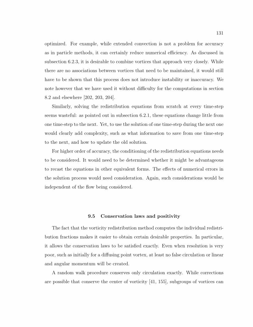
131

optimized. For example, while extended convection is not a problem for accuracy

as in particle methods, it can certainly reduce numerical efficiency. As discussed in

subsection 6.2.3, it is desirable to combine vortices that approach very closely. While

there are no associations between vortices that need to be maintained, it would still

have to be shown that this process does not introduce instability or inaccuracy. We

note however that we have used it without difficulty for the computations in section

8.2 and elsewhere [202, 203, 204].

Similarly, solving the redistribution equations from scratch at every time-step

seems wasteful: as pointed out in subsection 6.2.1, these equations change little from

one time-step to the next. Yet, to use the solution of one time-step during the next one

would clearly add complexity, such as what information to save from one time-step

to the next, and how to update the old solution.

For higher order of accuracy, the conditioning of the redistribution equations needs

to be considered. It would need to be determined whether it might be advantageous

to recast the equations in other equivalent forms. The effects of numerical errors in

the solution process would need consideration. Again, such considerations would be

independent of the flow being considered.

9.5 Conservation laws and positivity

The fact that the vorticity redistribution method computes the individual redistri-

bution fractions makes it easier to obtain certain desirable properties. In particular,

it allows the conservation laws to be satisfied exactly. Even when resolution is very

poor, such as initially for a diffusing point vortex, at least no false circulation or linear

and angular momentum will be created.

A random walk procedure conserves only circulation exactly. While corrections

are possible that conserve the center of vorticity [41, 155], subgroups of vortices can

132

still perform an appreciable net motion without a physical mechanism causing it.

The particle scheme proposed by Fishelov [78] is not conservative unless a corrected

rule is used to perform the integrations in her convolution, but the potential high-

order of accuracy may make this unimportant. The particle methods do not satisfy

conservation of center of vorticity exactly when the particle distribution becomes

nonuniform.

Another advantage of the redistribution equations is that they tend to localize

the errors in velocity that result from the numerical diffusion. To be precise, the

redistribution equations ensure that the leading order decay terms of the error in

velocity vanish exactly.

Another desirable property is the positivity of the redistribution fractions; it as-

sures that regardless of numerical inaccuracy, no false reversed vorticity is created.

Whether particle methods satisfy this constraint depends on factors such as the choice

of smoothing function and of the time discretization. For example, Fishelov’s method

does not satisfy positivity and can generate reversed vorticity, although the amount

should be very small if the vorticity distribution is sufficiently smooth. The inte-

gral constraints given by Degond and Mas-Gallic [72] show that third-order accurate

particle schemes do not satisfy positivity.

It may seem surprising that for the Stokes equations the vorticity redistribution

method can achieve any order of accuracy with positive fractions, while the particle

methods cannot. The reason is that the vorticity redistribution method discretizes

convection for a finite time-step, rather than an infinitesimal one. In particular, if we

let the time-step tend to zero in the vorticity redistribution method, while keeping

the location of the vortices fixed, the scaled spacing between the vortices would tend

to infinity. In Appendix A it is shown that the redistribution equations do not have

a positive third-order solution if the scaled spacing is more than a finite value. Thus

high order of accuracy can only be achieved for a finite time-step.

133

For the Navier-Stokes equations a finite time-step is a mixed blessing; the splitting

into viscous and inviscid steps should not introduce an error larger than the spatial

order of accuracy. Note however that the time-step is an order smaller than the spatial

resolution. In an unbounded domain, Strang splitting with reversal of the order of

the steps [19] would be fourth-order accurate with respect to space.

In the next chapter, we will present the conclusions about our work and also

suggest some areas for further work on our vorticity redistribution method.

CHAPTER 10

CONCLUSIONS

In this thesis, we have developed a mesh-free, accurate numerical method, called

the ‘vorticity redistribution method’, for handling diffusion in vortex methods for

incompressible flows.

By construction, our vorticity redistribution method might be considered to be a

computed finite difference formula for vortices with disordered locations. Our inten-

tion was to design a method with the same independent computational points as the

random walk method. This gives it the capability to handle complex separated flows

that may be impractical using other schemes. It also allows the computational points

to truly follow very strong convection processes. This may be crucial to compute flows

with unsteady boundary layer separation [241]. Yet at the same time we wanted to

avoid the large and awkward numerical errors in the random walk method.

Our new procedure has been tremendously successful in this quest. The results of,

especially, section 8.2 provide overwhelming evidence that our method maintains the

advantages of the random walk method, but with a dramatic increase in accuracy.

Wang [245] complained that the large and random errors in the random walk methods

(such as those between figures 8.22(a) and (b)) made the study of the effects of the

true physical parameters very difficult. Our new method now allows such practical

applications.

In fact, as discussed in subsection 8.2.9, the evidence suggests that our results for

the impulsively translated circular cylinder at Re = 9, 500 may surpass all available

finite difference results. Yet, such schemes are clearly less flexible, and some use as

much as half a million mesh points where we needed 60,000 vortices. Of course, the

CPU time per vortex can be expected to be much larger than the time per mesh

134

135

point in a finite difference computation, especially for this simple geometry. In any

case, of all computations, our results agreed closest with the preliminary spectral

element results of Kruse & Fischer [120] who used half a million nodal points in half

the flow region. Spectral methods are of course targeted to very different conditions

than our mesh-free method. We also showed that our method works equally well in

three dimensions as in two.

We further explained that it has significant further theoretical advantages over

other vortex methods in addition to the fact that it is mesh-free. Our method can

show a better performance for small scale phenomena; compare the discussion about a

diffusing point vortex in section 9.1. This reduces the number of vortices needed. Our

method uses its vortices also very efficiently since they are distributed only where there

is vorticity; hence our method uses still less vortices than other methods. Our method

adds new vortices automatically when the vorticity diffuses toward new locations or

where straining depletes regions of vortices. Particle methods periodically restore the

vortex distribution, interpolating the vorticity of the new distribution from the old.

This introduces complexity as well as interpolation errors.

Other advantages of our method are that the conservation laws are satisfied ex-

actly, and that our method can preserve the sign of the vorticity exactly even at high

orders of accuracy. Another significant advantage is that there are few computational

parameters in our method, and they are easy to choose. We further never needed to

“adjust” our parameters; this makes our method highly reliable.

While Fishelov’s method [78] can easily achieve spectral accuracy, our method

cannot. On the other hand, there is also no fundamental limitation on the order of

accuracy that can be achieved by our method. However, more than first order accu-

racy has not yet been demonstrated in actual computations. Also accuracy beyond

fourth order is not completely trivial since it requires additional consideration of the

time splitting error.

136

The computational time required for the vorticity redistribution method is of the

order of the time required for convection. In typical computations based on particle

methods, on the other hand, the computational time needed for diffusion is small

compared to the time needed for convection. However, at least for the case of the

impulsively translated cylinder at Re = 9, 500, the particle methods use much more

vortices and hence the time required for redistribution seems not really relevant for

that flow. In addition, we must point out that so far we have not made any serious

attempt to reduce our computational time. We certainly have no doubt that the

various brute force approaches we have followed so far are unnecessarily inefficient.

Since we solve two identical diffusion problems back to back, a factor 2 reduction in

time would be trivial at the expense of additional storage. Interestingly, in theory the

reduction in computational effort could still be arbitrarily (“infinitely”) large. Future

studies will have to determine how much of that is really possible.

In addition to improving the computational time, further work on the vorticity re-

distribution method may be continued in many ways. One is to extend the method to

handle different boundary conditions; for example, free-surface and periodic boundary

conditions. In section 7.3 the method was applied to three-dimensional Stokes flows;

this work could be continued to flows including convection, and to flows with no-slip

or other boundary conditions. Finally, one could also investigate the feasibility of

extending the redistribution method to compressible flows. The fact that it is in fact

a computed finite difference formula suggests a wide further range of applicability.

137

Figure 4.1: Redistribution of the circulation of a vortex Γni .

138

Figure 6.1: Vortex pair, Re = 0: Growth in number of computational vortices for the

Stokes flow starting from a pair of counter-rotating point vortices. The small circle

indicates the size of the computational neighborhood of a typical vortex.

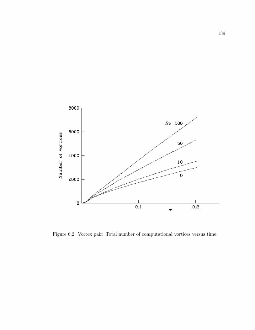
139

Figure 6.2: Vortex pair: Total number of computational vortices versus time.

140

Figure 6.3: Vortex pair, Re = 50: Growth in number of computational vortices for

a flow starting from a pair of counter-rotating point vortices at Re = 50. The small

circle indicates the size of the computational neighborhood of a typical vortex.

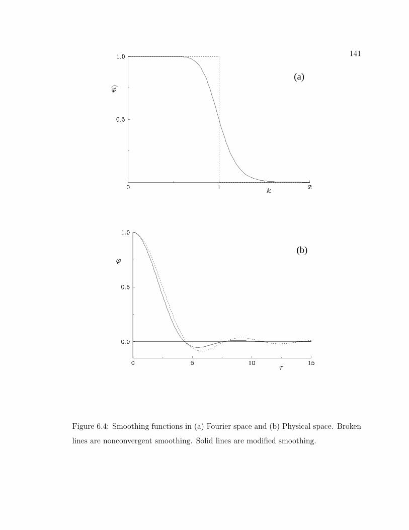
141

(a)

(b)

Figure 6.4: Smoothing functions in (a) Fourier space and (b) Physical space. Broken

lines are nonconvergent smoothing. Solid lines are modified smoothing.

142

Figure 7.1: Point vortex, Re = 50: Growth in mean square radius of a single diffusing

vortex. The solid line is exact and circles are vorticity redistribution solutions.

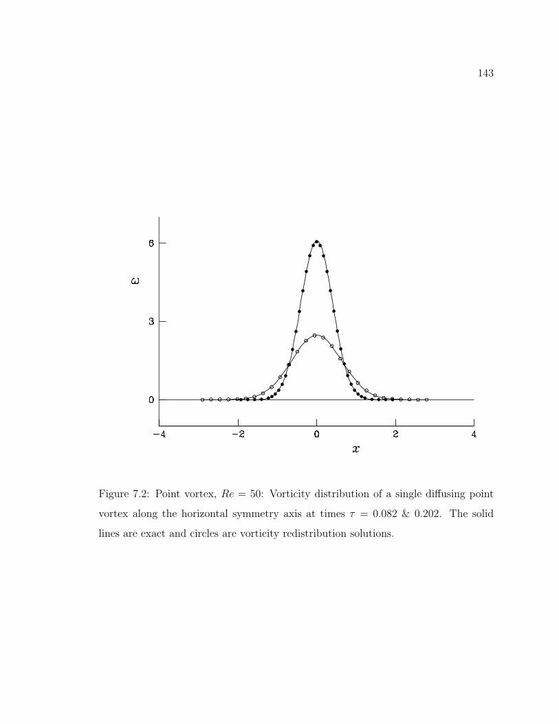
143

Figure 7.2: Point vortex, Re = 50: Vorticity distribution of a single diffusing point

vortex along the horizontal symmetry axis at times τ = 0.082 & 0.202. The solid

lines are exact and circles are vorticity redistribution solutions.

144

Figure 7.3: Vortex pair, Re = 0: Vorticity along the connecting line at times τ = 0.082

& 0.202. The solid lines are exact and circles are vorticity redistribution solutions.

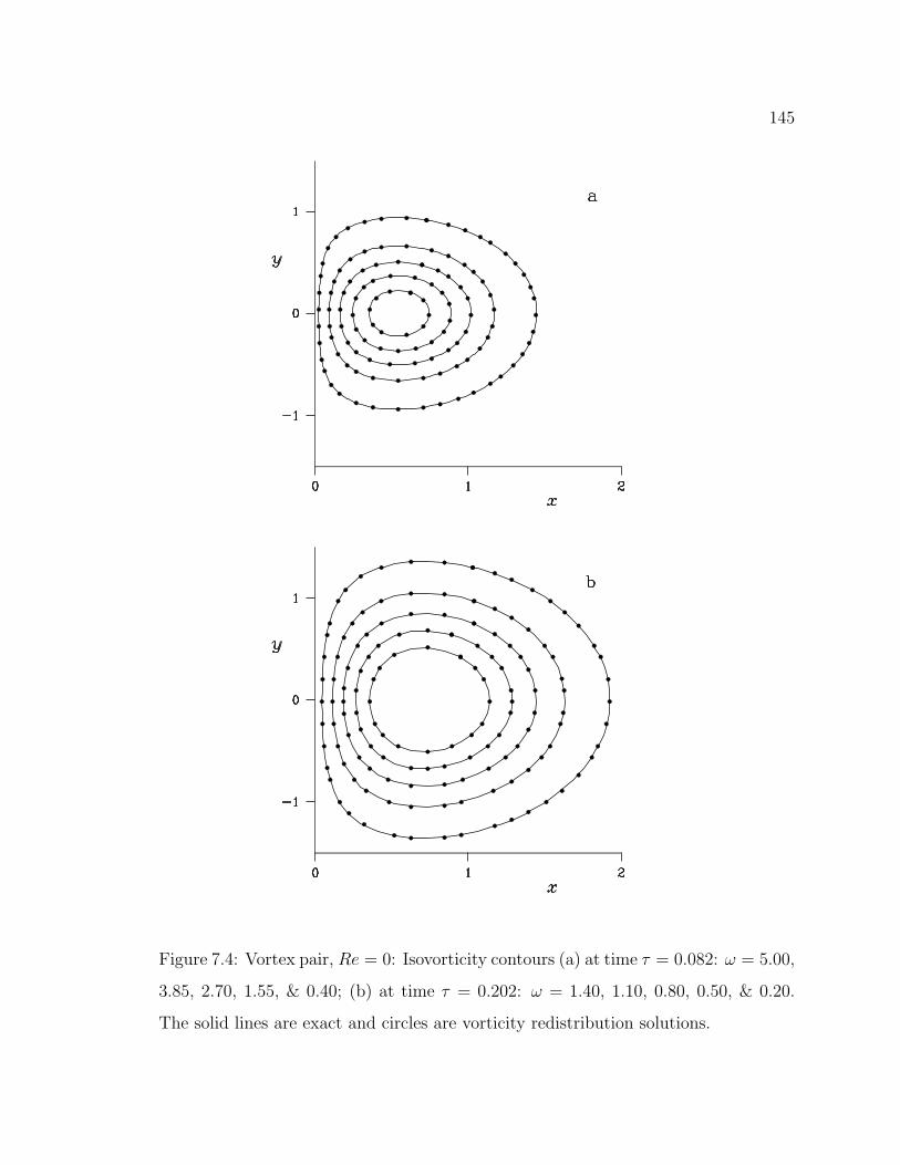
145

Figure 7.4: Vortex pair, Re = 0: Isovorticity contours (a) at time τ = 0.082: ω = 5.00,

3.85, 2.70, 1.55, & 0.40; (b) at time τ = 0.202: ω = 1.40, 1.10, 0.80, 0.50, & 0.20.

The solid lines are exact and circles are vorticity redistribution solutions.

146

Figure 7.5: Vortex pair, Re = 50: Isovorticity contours for a counter-rotating vortex

pair. (a) at time τ = 0.01025: ω = 40, 24, & 8; (b) at time τ = 0.02050: ω = 20, 12,

& 4. The dashed and solid lines represent orders of approximation in the analytical

solution. Circles are vorticity redistribution solutions.

147

Figure 7.6: Vortex pair, Re = 50: The effect of using exponentially decaying core

shapes instead of algebraically decaying ones.

148

Figure 7.7: Vortex pair: Isovorticity contours ω = 5, 3, & 1 at time τ = 0.082 for

different Reynolds numbers.

149

Figure 7.8: Vortex pair: Isovorticity contours ω = 1.7, 1.5, . . . , 0.1 at time τ = 0.202

for different Reynolds numbers.

150

Figure 7.9: Vortex pair: Maximum vorticity for different Reynolds numbers. Stokes

represents the exact solution for Re = 0.

151

Figure 7.10: Vortex pair: Distance of the point of maximum vorticity from the sym-

metry plane. Stokes represents the exact solution for Re = 0.

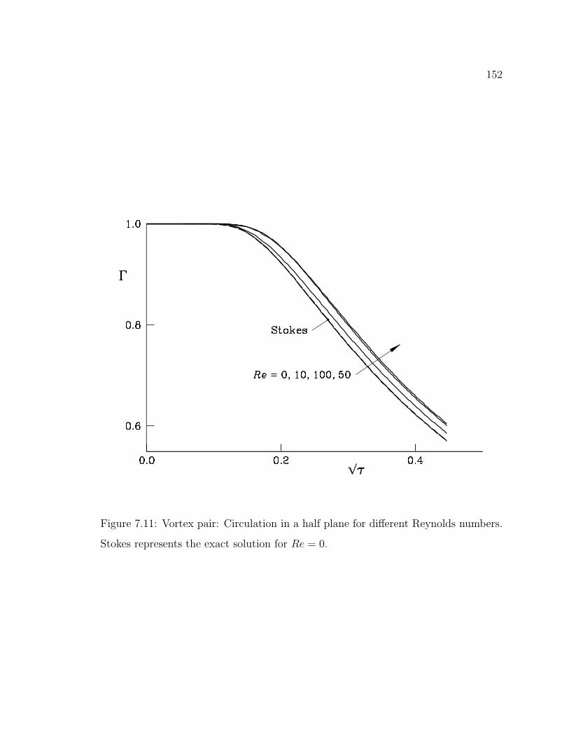
152

Figure 7.11: Vortex pair: Circulation in a half plane for different Reynolds numbers.

Stokes represents the exact solution for Re = 0.

153

Figure 7.12: Vortex pair: Average velocity v, vortex center velocity vc, and asymptotic

velocity vg for vanishing Reynolds number. Short dash curves and dot dash curves

represent the small time and the long time analytical solutions respectively.

154

Figure 7.13: Vortex pair: Deviation in average velocity v from the inviscid drift

velocity. Short dash curves represent the small time analytical solutions. Stokes

represents the exact solution for Re = 0 and the asymptotic solution for large time

for any Reynolds number.

155

Figure 7.14: Vortex pair: Deviation in vortex center velocity vc from the inviscid

drift velocity. Short dash curves represent the small time analytical solutions. Stokes

represents the exact solution for Re = 0 and the asymptotic solution for large time

for any Reynolds number.

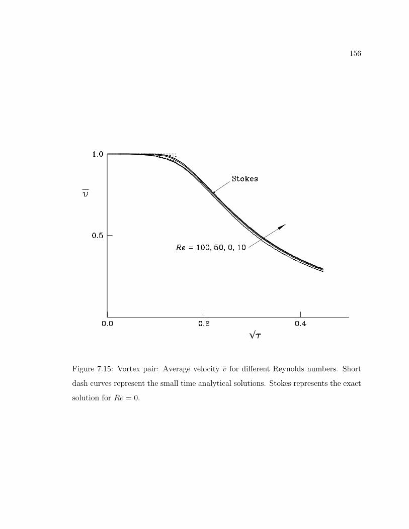
156

Figure 7.15: Vortex pair: Average velocity v for different Reynolds numbers. Short

dash curves represent the small time analytical solutions. Stokes represents the exact

solution for Re = 0.

157

Figure 7.16: Vortex pair: Vortex center velocity vc for different Reynolds numbers.

Short dash curves represent the small time analytical solutions. Stokes represents the

exact solution for Re = 0.

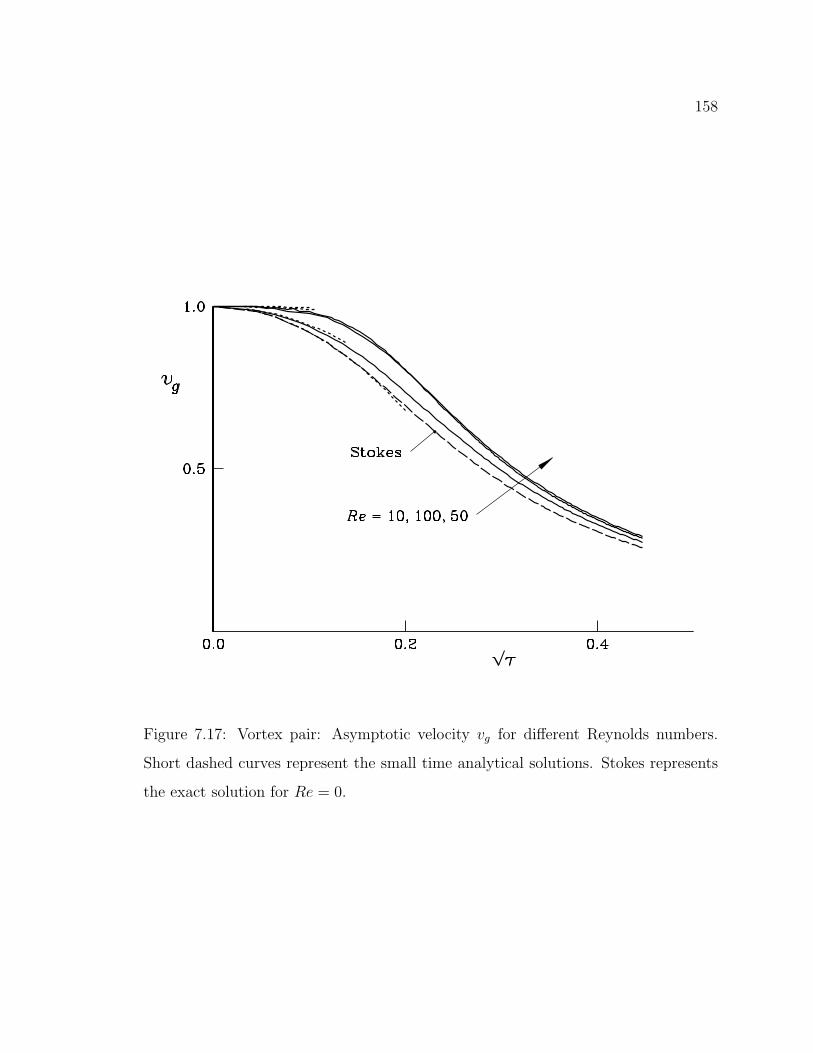
158

Figure 7.17: Vortex pair: Asymptotic velocity vg for different Reynolds numbers.

Short dashed curves represent the small time analytical solutions. Stokes represents

the exact solution for Re = 0.

159

Figure 7.18: Vortex pair: Average velocity v, vortex center velocity vc and asymptotic

velocity vg for Reynolds number 100.

160

(a)

(b)

Figure 7.19: Vorticity for three-dimensional diffusion of a pair of vortex poles: (a)

Along a line through the vortices; (b) Isovorticity contours ω=0.5, 1.0, 1.5, 2.0, &

2.5 in the plane of the vortices. Solid lines are exact and symbols are redistribution

solutions.

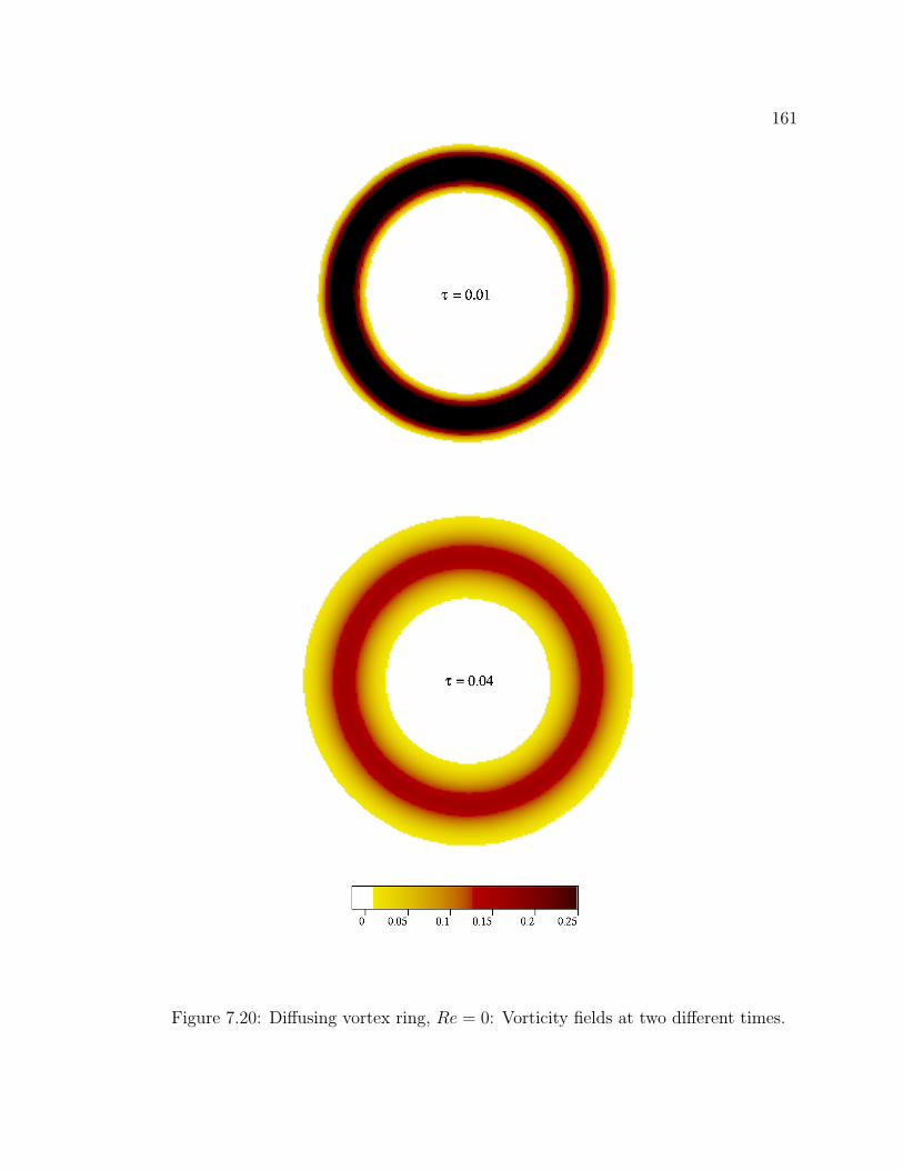
161

Figure 7.20: Diffusing vortex ring, Re = 0: Vorticity fields at two different times.

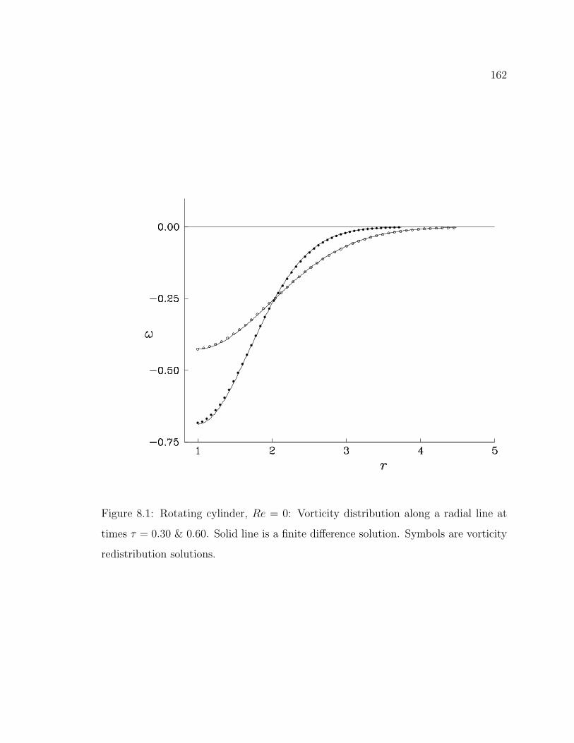
162

Figure 8.1: Rotating cylinder, Re = 0: Vorticity distribution along a radial line at

times τ = 0.30 & 0.60. Solid line is a finite difference solution. Symbols are vorticity

redistribution solutions.

163

Figure 8.2: Oscillating cylinder, Re = 0: Vorticity distribution along a radial line at

different times. Solid lines are finite difference solutions. Dashed lines are redistribu-

tion solutions.

Figure 8.3: Oscillating cylinder, Re = 0: Total circulation during one time period

of oscillation. Solid lines are finite difference solutions. Symbols are redistribution

solutions.

164

t = 1.00 t = 1.50

t = 2.00 t = 3.00

t = 4.00 t = 5.00

Figure 8.4: Impulsively translated cylinder, Re = 550: Instantaneous streamlines

from vorticity redistribution (∆t = 0.01; ǫΓ = 10−5); see subsection 8.2.2 for stream-

line values.

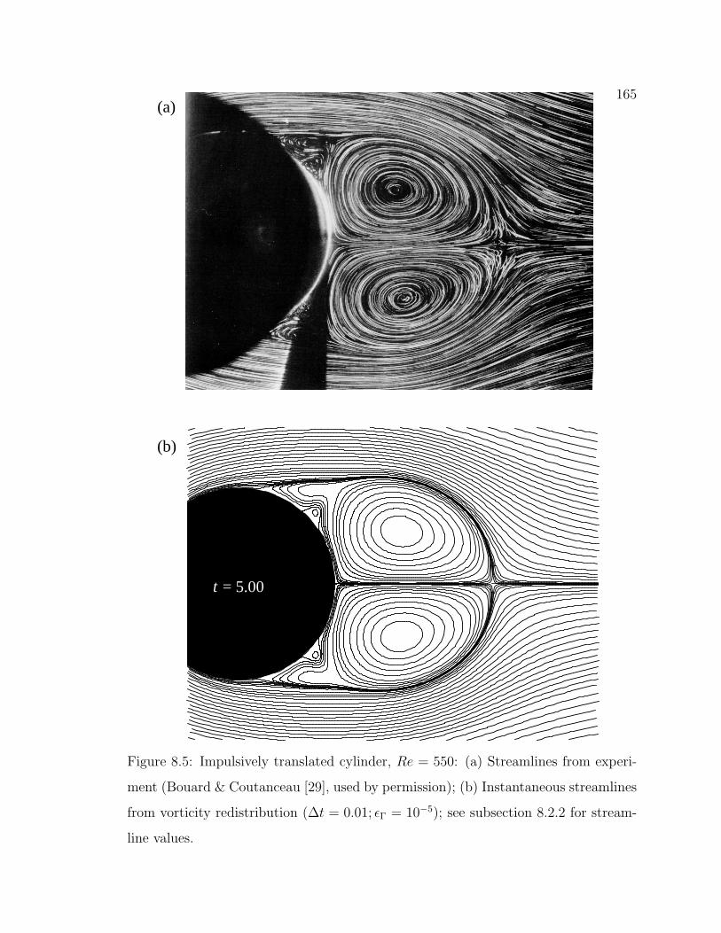
165(a)

(b)

t = 5.00

Figure 8.5: Impulsively translated cylinder, Re = 550: (a) Streamlines from experi-

ment (Bouard & Coutanceau [29], used by permission); (b) Instantaneous streamlines


line values.

166

t = 1.00 t = 1.50

t = 2.00 t = 3.00

t = 4.00 t = 5.00

Figure 8.6: Impulsively translated cylinder, Re = 3, 000: Instantaneous streamlines


line values.

167(a)

(b)

t = 5.00

Figure 8.7: Impulsively translated cylinder,Re = 3, 000: (a) Streamlines from experi-



line values.

168

(a) (b)

t = 1.50

t = 2.00

Figure 8.8: Impulsively translated cylinder, Re = 9, 500: (a) Streamlines from experi-



line values.

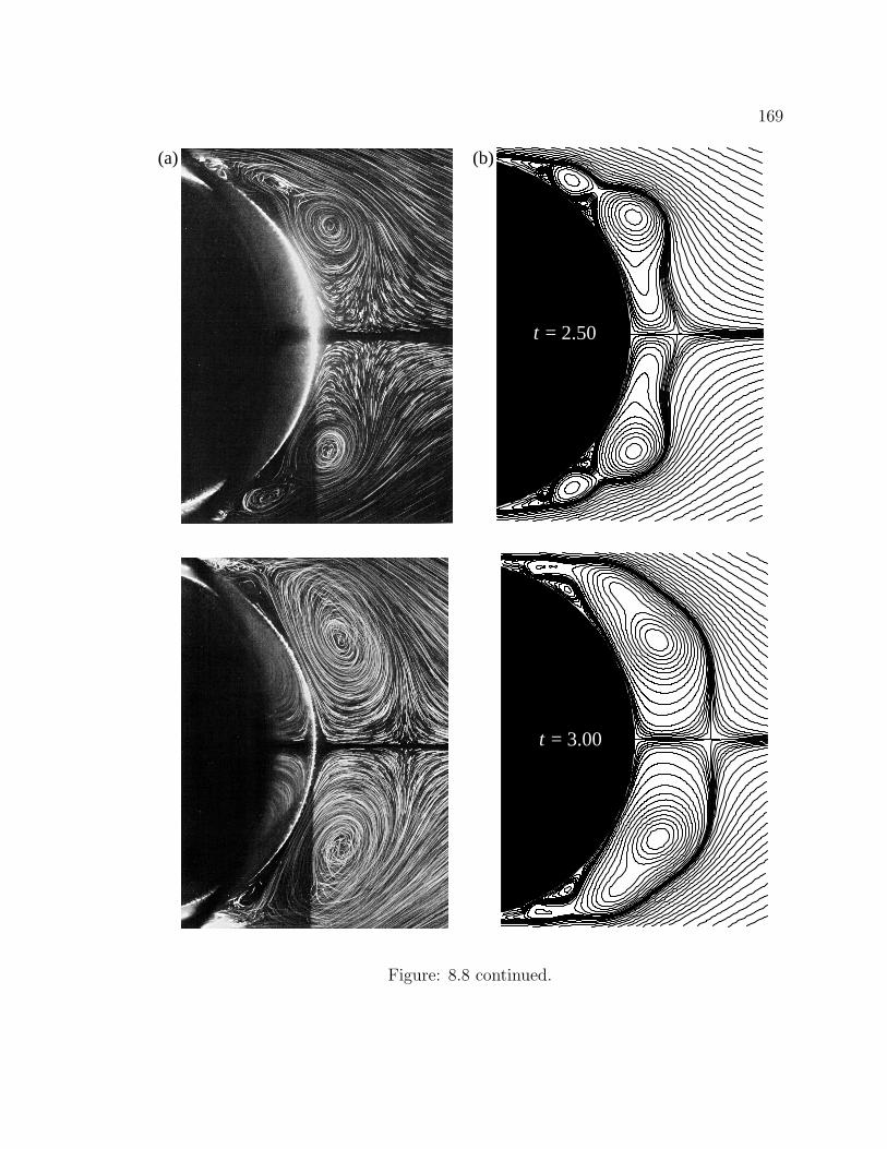
169

(a) (b)

t = 2.50

t = 3.00

Figure: 8.8 continued.

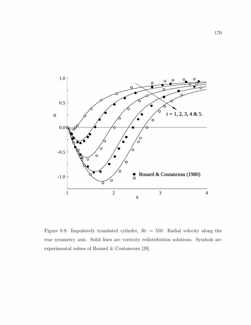
170

1 2 3 4

-1.0

-0.5

0.0

0.5

1.0

u

x

Bouard & Coutanceau (1980)

t = 1, 2, 3, 4 & 5.

Bouard & Coutanceau (1980)

t = 1, 2, 3, 4 & 5.

Figure 8.9: Impulsively translated cylinder, Re = 550: Radial velocity along the

rear symmetry axis. Solid lines are vorticity redistribution solutions. Symbols are

experimental values of Bouard & Coutanceau [29].

171

1 2 3 4

-1.0

-0.5

0.0

0.5

1.0

u

x

Pepin (1990)

t = 1, 2, 3, 4 & 5.

1 2 3 4

-1.0

-0.5

0.0

0.5

1.0

u

x

Loc (1980)

t = 1, 2, 3, 4 & 5.

Figure 8.10: Impulsively translated cylinder, Re = 550: Radial velocity along the


solutions computed by Pepin [170], and Loc [133].

172

1 2 3-1.5

-1.0

-0.5

0.0

0.5

1.0

u

x

Loc & Bouard (1985)

t = 1, 2, 3, 4 & 5.

Figure 8.11: Impulsively translated cylinder, Re = 3, 000: Radial velocity along the


experimental values of Loc & Bouard [134].

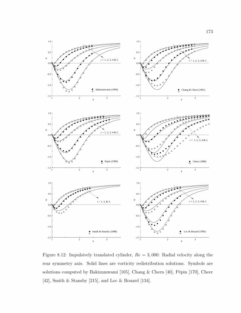
173

1 2 3-1.5

-1.0

-0.5

0.0

0.5

1.0

u

x

Hakizumwami (1994)

t = 1, 2, 3, 4 & 5.

1 2 3-1.5

-1.0

-0.5

0.0

0.5

1.0

u

x

Chang & Chern (1991)

t = 1, 2, 3, 4 & 5.

1 2 3-1.5

-1.0

-0.5

0.0

0.5

1.0

u

x

Pepin (1990)

t = 1, 2, 3, 4 & 5.

1 2 3-1.5

-1.0

-0.5

0.0

0.5

1.0

u

x

Cheer (1989)

t = 1, 2, 3, 4 & 5.

1 2 3-1.5

-1.0

-0.5

0.0

0.5

1.0

u

x

Smith & Stansby (1988)

t = 1, 2, & 3.

1 2 3-1.5

-1.0

-0.5

0.0

0.5

1.0

u

x

Loc & Bouard (1985)

t = 1, 2, 3, 4 & 5.



solutions computed by Hakizumwami [105], Chang & Chern [40], Pepin [170], Cheer

[42], Smith & Stansby [215], and Loc & Bouard [134].

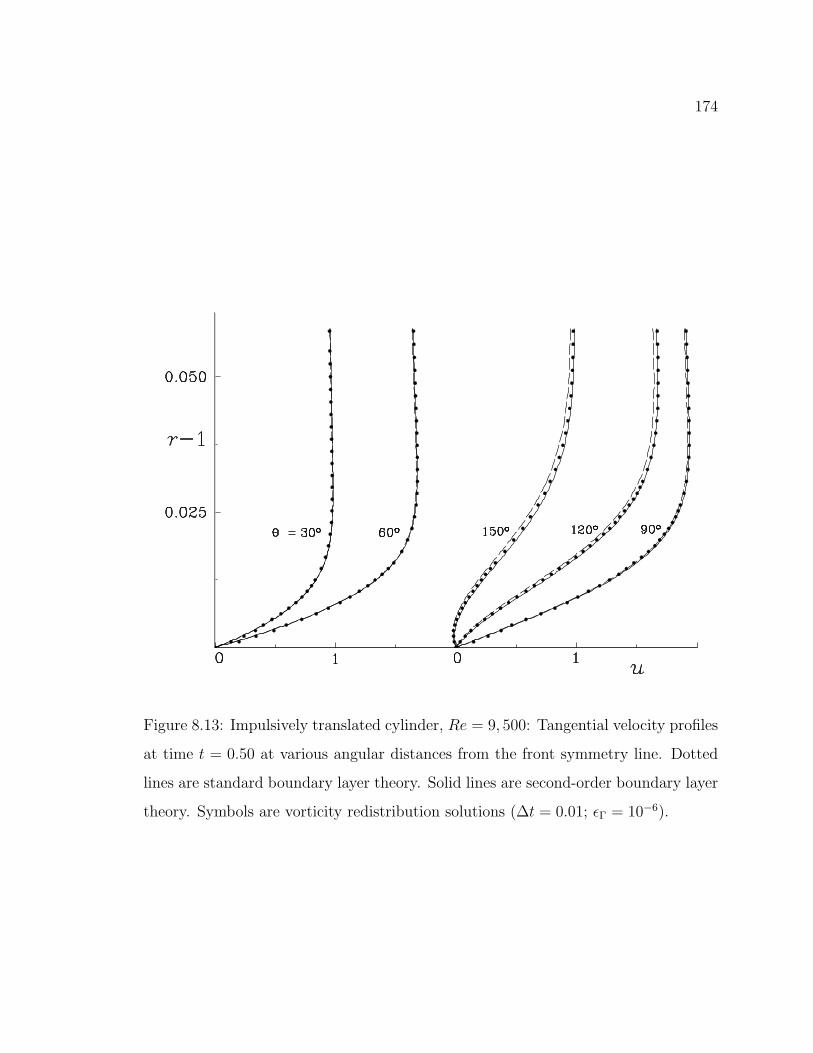
174

Figure 8.13: Impulsively translated cylinder, Re = 9, 500: Tangential velocity profiles

at time t = 0.50 at various angular distances from the front symmetry line. Dotted

lines are standard boundary layer theory. Solid lines are second-order boundary layer

theory. Symbols are vorticity redistribution solutions (∆t = 0.01; ǫΓ = 10−6).

175

1 2-0.5

0.0

0.5

1.0

u

x

Loc & Bouard (1985)

t = 1.2, 2.0 & 2.8.



experimental values of Loc & Bouard [134].

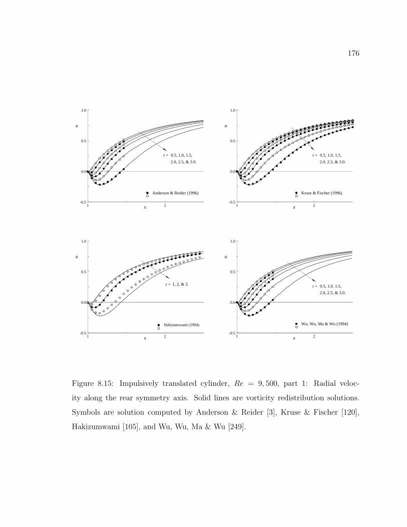
176

1 2-0.5

0.0

0.5

1.0

u

x

Anderson & Reider (1996)

t = 0.5, 1.0, 1.5,

2.0, 2.5, & 3.0.

1 2-0.5

0.0

0.5

1.0

u

x

Kruse & Fischer (1996)

t = 0.5, 1.0, 1.5,

2.0, 2.5, & 3.0.

1 2-0.5

0.0

0.5

1.0

u

x

Hakizumwami (1994)

t = 1, 2, & 3.

1 2-0.5

0.0

0.5

1.0

u

x

Wu, Wu, Ma & Wu (1994)

t = 0.5, 1.0, 1.5,

2.0, 2.5, & 3.0.

Figure 8.15: Impulsively translated cylinder, Re = 9, 500, part 1: Radial veloc-

ity along the rear symmetry axis. Solid lines are vorticity redistribution solutions.

Symbols are solution computed by Anderson & Reider [3], Kruse & Fischer [120],

Hakizumwami [105], and Wu, Wu, Ma & Wu [249].

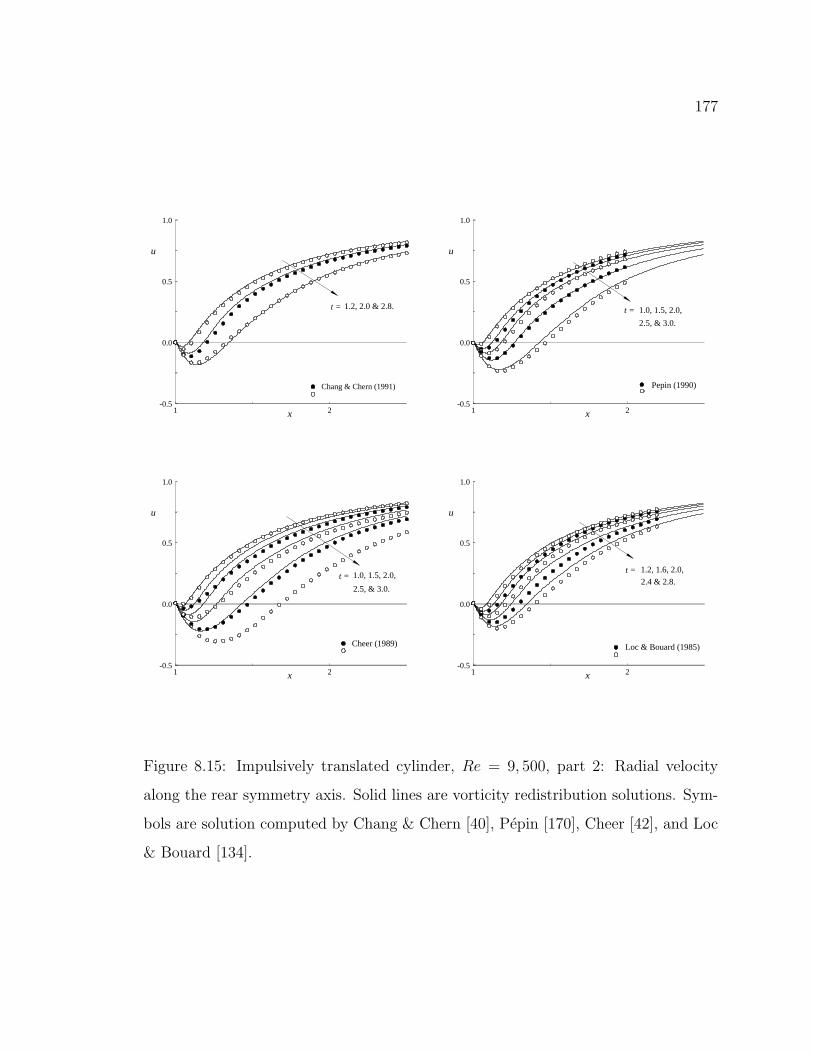
177

1 2-0.5

0.0

0.5

1.0

u

x


t = 1.2, 2.0 & 2.8.

1 2-0.5

0.0

0.5

1.0

u

x

Pepin (1990)

t = 1.0, 1.5, 2.0,

2.5, & 3.0.

1 2-0.5

0.0

0.5

1.0

u

x

Cheer (1989)

t = 1.0, 1.5, 2.0,

2.5, & 3.0.

1 2-0.5

0.0

0.5

1.0

u

x

Loc & Bouard (1985)

t = 1.2, 1.6, 2.0,

2.4 & 2.8.

Figure 8.15: Impulsively translated cylinder, Re = 9, 500, part 2: Radial velocity

along the rear symmetry axis. Solid lines are vorticity redistribution solutions. Sym-

bols are solution computed by Chang & Chern [40], Pepin [170], Cheer [42], and Loc

& Bouard [134].

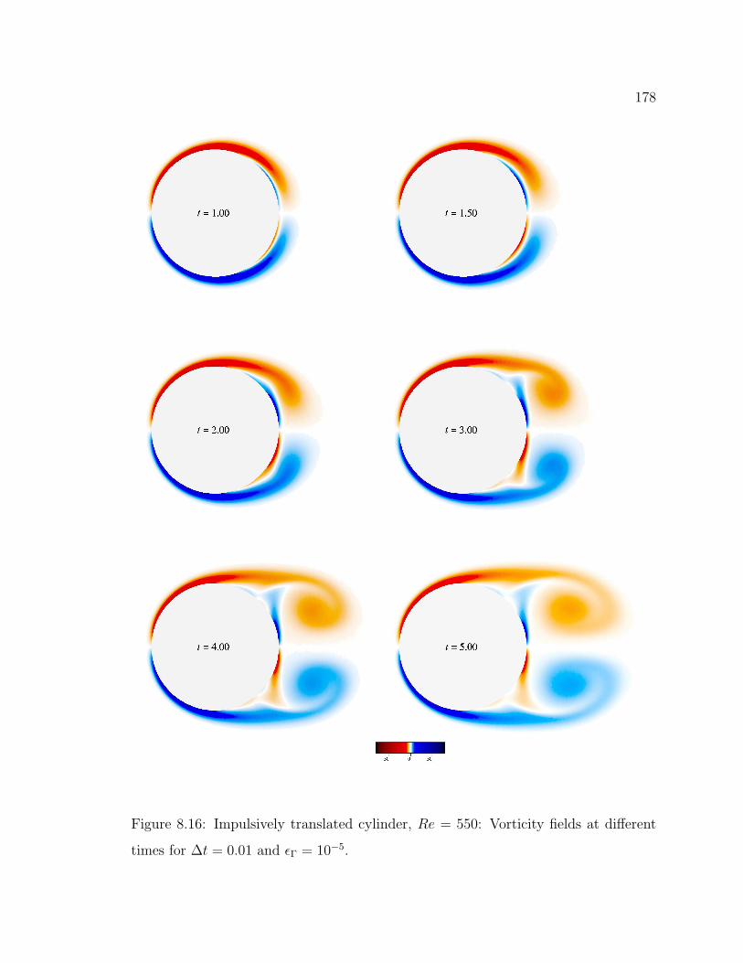
178

Figure 8.16: Impulsively translated cylinder, Re = 550: Vorticity fields at different

times for ∆t = 0.01 and ǫΓ = 10−5.

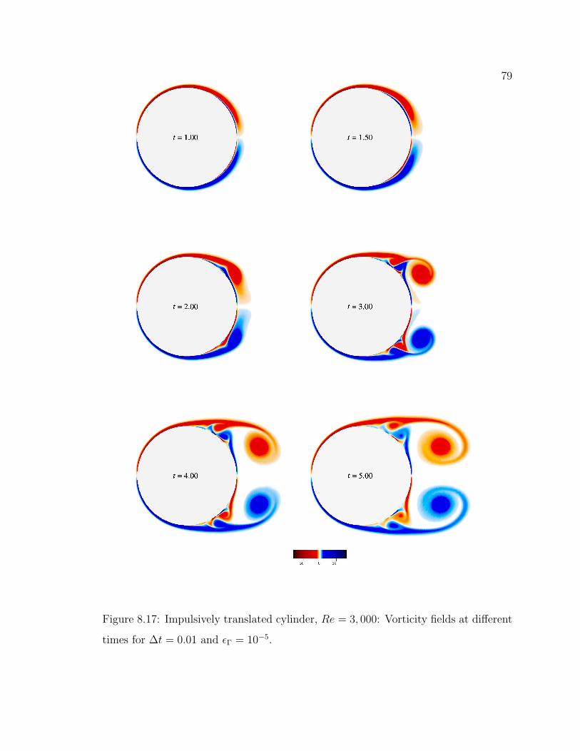
179

Figure 8.17: Impulsively translated cylinder, Re = 3, 000: Vorticity fields at different


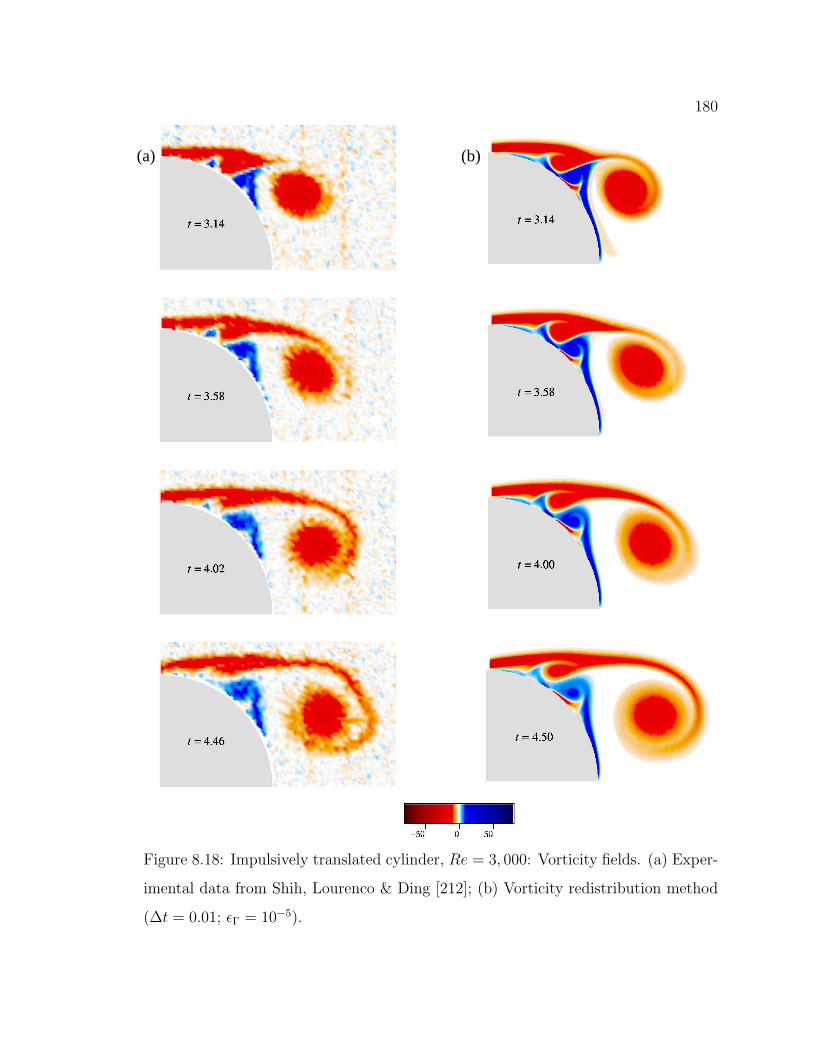
180

(a) (b)

Figure 8.18: Impulsively translated cylinder, Re = 3, 000: Vorticity fields. (a) Exper-

imental data from Shih, Lourenco & Ding [212]; (b) Vorticity redistribution method

(∆t = 0.01; ǫΓ = 10−5).

181



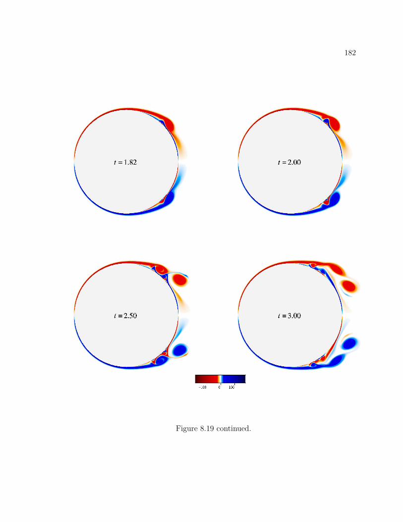
182

Figure 8.19 continued.

183

(a) (b)

Figure 8.20: Impulsively translated cylinder, Re = 9, 500: Vorticity fields. (a) Spec-

tral element method (preliminary data of Kruse & Fischer [120], used by kind per-

mission); (b) Vorticity redistribution method (∆t = 0.01; ǫΓ = 10−6).

184

(a) (b)

Figure 8.21: Impulsively translated cylinder, Re = 9, 500: Vorticity fields. (a) Particle

strength exchange method (Koumoutsakos & Leonard [117], used by permission); (b)

Vorticity redistribution method (∆t = 0.01; ǫΓ = 10−6).

185

t = 2.00 t = 2.00

t = 1.50 t = 1.50

(a) (b)

Figure 8.22: Impulsively translated cylinder, Re = 10, 000: Vorticity fields obtained

from random walk computations (Unpublished data of Van Dommelen, used by per-

mission); (a) and (b) refer to two different runs of the computation.

186

t = 3.00 t = 3.00

t = 2.50 t = 2.50

(a) (b)


187

(a) (b)


times for ∆t = 0.01 and ǫΓ = 5 × 10−7.

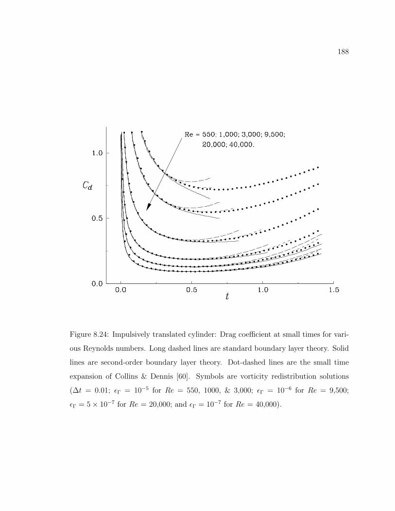
188

Figure 8.24: Impulsively translated cylinder: Drag coefficient at small times for vari-

ous Reynolds numbers. Long dashed lines are standard boundary layer theory. Solid

lines are second-order boundary layer theory. Dot-dashed lines are the small time

expansion of Collins & Dennis [60]. Symbols are vorticity redistribution solutions

(∆t = 0.01; ǫΓ = 10−5 for Re = 550, 1000, & 3,000; ǫΓ = 10−6 for Re = 9,500;

ǫΓ = 5 × 10−7 for Re = 20,000; and ǫΓ = 10−7 for Re = 40,000).

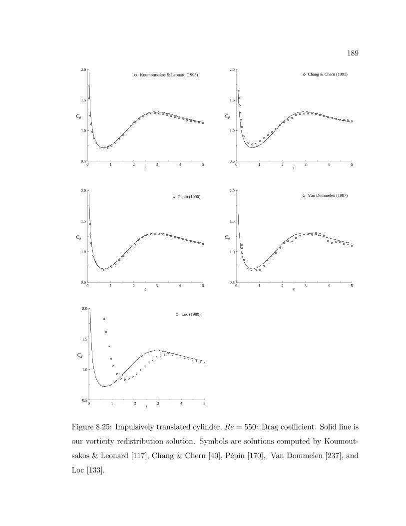
189

0 1 2 3 4 50.5

1.0

1.5

2.0

Cd

t

Koumoutsakos & Leonard (1995)

0 1 2 3 4 50.5

1.0

1.5

2.0

Cd

t


0 1 2 3 4 50.5

1.0

1.5

2.0

Cd

t

Pepin (1990)

0 1 2 3 4 50.5

1.0

1.5

2.0

Cd

t

Van Dommelen (1987)

0 1 2 3 4 50.5

1.0

1.5

2.0

Cd

t

Loc (1980)

Figure 8.25: Impulsively translated cylinder, Re = 550: Drag coefficient. Solid line is

our vorticity redistribution solution. Symbols are solutions computed by Koumout-

sakos & Leonard [117], Chang & Chern [40], Pepin [170], Van Dommelen [237], and

Loc [133].

190

0 1 2 3 4 5

0.0

0.5

1.0

1.5

Cd

t

Re = 550

C l

Figure 8.26: Impulsively translated cylinder, Re = 550: Drag and lift coefficients.

Solid lines are vorticity redistribution solutions (∆t = 0.01; ǫΓ = 10−6). The short

and long dashed lined are random walk results of Van Dommelen [237] at ∆t = 0.0125

and ∆t = 0.025 respectively.

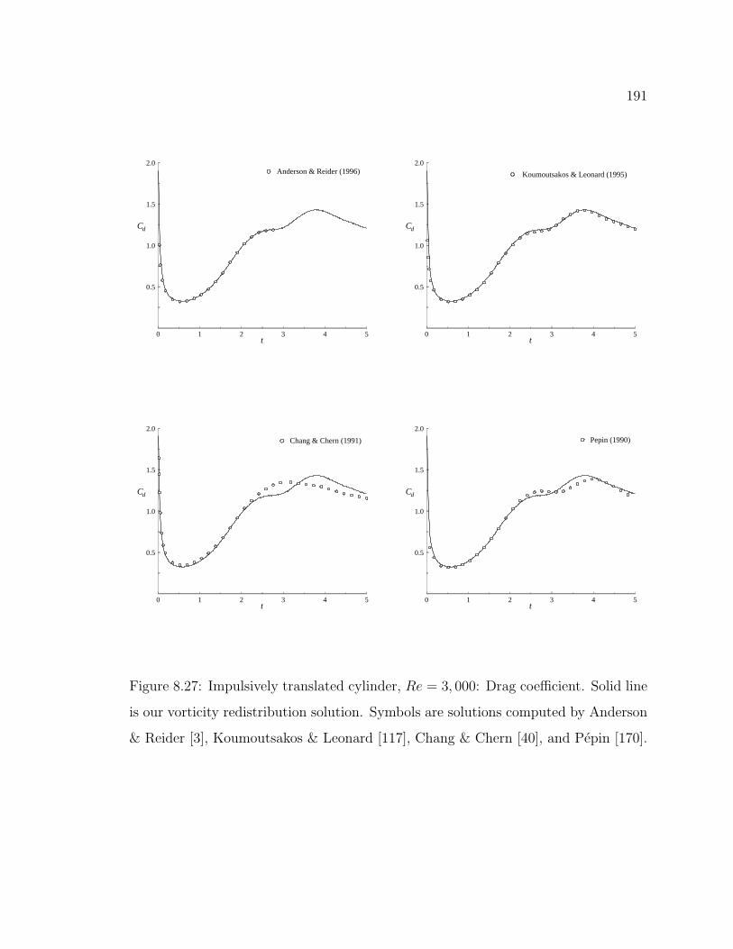
191

0 1 2 3 4 5

0.5

1.0

1.5

2.0

Cd

t


0 1 2 3 4 5

0.5

1.0

1.5

2.0

Cd

t


0 1 2 3 4 5

0.5

1.0

1.5

2.0

Cd

t


0 1 2 3 4 5

0.5

1.0

1.5

2.0

Cd

t

Pepin (1990)

Figure 8.27: Impulsively translated cylinder, Re = 3, 000: Drag coefficient. Solid line

is our vorticity redistribution solution. Symbols are solutions computed by Anderson

& Reider [3], Koumoutsakos & Leonard [117], Chang & Chern [40], and Pepin [170].

192

0 1 2 3

0.5

1.0

1.5

Cd

t


0 1 2 3

0.5

1.0

1.5

Cd

t

Kruse & Fischer (1996)

0 1 2 3

0.5

1.0

1.5

Cd

t


0 1 2 3

0.5

1.0

1.5

Cd

t

Wu, Wu, Ma, & Wu (1994)

Figure 8.28: Impulsively translated cylinder, Re = 9, 500, part 1: Drag coefficient.

Solid line is our vorticity redistribution solution. Symbols are solutions computed by

Anderson & Reider [3], Kruse & Fischer [120], Koumoutsakos & Leonard [117], and

Wu, Wu, Ma & Wu [249].

193

0 1 2 3

0.5

1.0

1.5

Cd

t


0 1 2 3

0.5

1.0

1.5

Cd

t

Pepin (1990)

0 1 2 3

0.5

1.0

1.5

Cd

t

Van Dommelen (1987)

Figure 8.28: Impulsively translated cylinder, Re = 9, 500, part 2: Drag coefficient.

Solid line is our vorticity redistribution solution. Symbols are solutions computed by

Chang & Chern [40], Pepin [170], and Van Dommelen (unpublished).

194

0 1 2 30.0

0.5

1.0

1.5

t

Cd

Re = 9,500

Figure 8.29: Impulsively translated cylinder, Re = 9, 500: Drag coefficient. Long

dashed line is ∆t = 0.04. Short dashed line is ∆t = 0.02. Solid line is ∆t = 0.01. For

all three cases ǫΓ = 10−6.

195

0 1 20.00

0.25

0.50

t

Cd

Re = 20,000

Figure 8.30: Impulsively translated cylinder, Re = 20, 000: Drag coefficient. Long

dashed line is ∆t = 0.04. Short dashed line is ∆t = 0.02. Solid line is ∆t = 0.01. For

all three cases ǫΓ = 5 × 10−7.

196

Figure 8.31: Impulsively translated cylinder, Re = 9, 500: Radial velocity along

the rear symmetry line at time t = 0.50. Dashed line is standard boundary layer

theory. Solid line is second-order boundary layer theory. Solid symbols are vorticity

redistribution solutions for ∆t = 0.01 and ǫΓ = 10−6. Open symbols are vorticity

redistribution solutions for ∆t = 0.01 and ǫΓ = 10−5. Dash-dot line is the irrotational

flow solution.

197

1.0 1.5

-0.25

0.00

0.25

u

x

t = 1.0, 1.5, 2.0,2.5, & 3.0.


rear symmetry axis. Short dashed lines are computed velocity using ∆t = 0.01 and

ǫΓ = 10−5. Solid lines are computed velocity using ∆t = 0.01 and ǫΓ = 10−6.

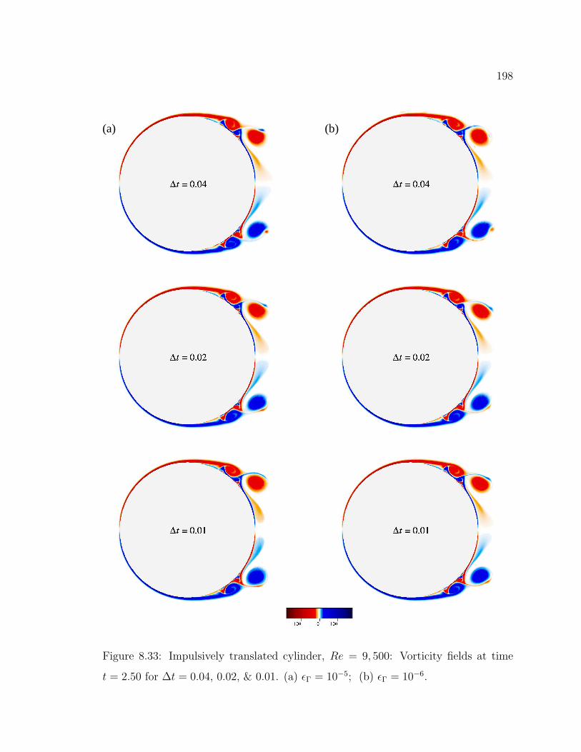
198

(a) (b)

Figure 8.33: Impulsively translated cylinder, Re = 9, 500: Vorticity fields at time

t = 2.50 for ∆t = 0.04, 0.02, & 0.01. (a) ǫΓ = 10−5; (b) ǫΓ = 10−6.

199

(a) (b)

Figure 8.34: Impulsively translated cylinder, Re = 9, 500: Vorticity fields at time

t = 3.00 for ∆t = 0.04, 0.02, & 0.01. (a) ǫΓ = 10−5; (b) ǫΓ = 10−6.

200

Figure 8.35: Impulsively translated cylinder, Re = 9, 500: Vorticity fields obtained

in particle strength exchange computation (preliminary data of Shiels [208], used by

kind permission); ∆t = 0.005, cut-off vorticity = 10−4 and Gaussian kernel size = 1.1

times the average particle spacing.

201

0 1 2 30.0

0.5

1.0

1.5

t

Cd

Re = 9,500

0 1 2 30.0

0.5

1.0

1.5

t

Cd

Re = 9,500

(a)

(b)

Figure 8.36: Impulsively translated cylinder, Re = 9, 500: Drag. (a) Solid line is

∆t = 0.01 and ǫΓ = 10−6. Short dashed line is ∆t = 0.01 and ǫΓ = 10−5. (b) Solid

line is ∆t = 0.01 and ǫΓ = 10−6. Dot-dashed line is ∆t = 0.02 and ǫΓ = 10−5. Long

dashed line is ∆t = 0.04 and ǫΓ = 10−5.

202

(a)

(b)

(c)

Figure 8.37: Impulsively translated cylinder: (a) Local vorticity contours obtained

from the Van Dommelen & Shen singularity [241]; (b) and (c) local vorticity fields at

t = 1.50 for Re = 9, 500 and Re = 20, 000 obtained from the vorticity redistribution

method.

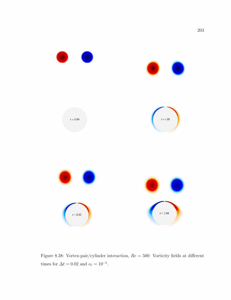
203

Figure 8.38: Vortex-pair/cylinder interaction, Re = 500: Vorticity fields at different


204


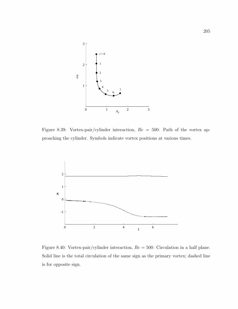
205

0 1 2 3

1

2

3

1

56

t = 0

xc

yc

7

2

3

4

Figure 8.39: Vortex-pair/cylinder interaction, Re = 500: Path of the vortex ap-

proaching the cylinder. Symbols indicate vortex positions at various times.

0 2 4 6

-1

0

1

2

t

κ

Figure 8.40: Vortex-pair/cylinder interaction, Re = 500: Circulation in a half plane.

Solid line is the total circulation of the same sign as the primary vortex; dashed line

is for opposite sign.

206

t = 0.00

t = 7.00

Figure 8.41: Vortex-pair/cylinder interaction, Re = 500: Computational vortices at

time t = 0.00 and t = 7.00.

APPENDIX A

DETAILED DERIVATIONS

This appendix gives some derivations mentioned earlier in the various chapters.

First is the derivation of the redistribution equations (4.8) and following. We write

the difference between the Fourier transform of the redistributed vorticity (4.5) and

the exactly diffused vorticity (4.6) in terms of the viscous scale hv =√ν∆t and the

scaled relative positions (4.7):

ωn+1 − ωn+1e = φ(kδ)

∑

i

Γni e

−i~k·~xi

∑

j

fnije

−ihv~k·~ξij − e−h2

vk2

. (A.1)

In the redistribution method, this error is made small of order O(hvk)M+2, or

O(∆t)(M+2)/2 for any finite wavenumber k, by equating the Taylor series expansions of

the two terms within the parentheses to that order. This produces, for anym ≤M+1,

∑

j

fnij (k1ξ1ij + k2ξ2ij)

m = 0 (m odd) ,

=m!

(12m)!

(k21 + k2

2)1

2m (m even) . (A.2)

Expanding using the binomial theorem, the individual equations become, for m1 +

m2 ≤M + 1,

∑

j

fnijξ

m1

1ij ξm2

2ij = 0 (m1 or m2 odd) ,

=m1!m2!

(12m1)!(

12m2)!

(m1 and m2 even) . (A.3)

These are the redistribution equations written out in (4.8) and following.

The remaining error in the Fourier transform, needed in chapter 5, is according

to the Taylor series remainder theorem

ωn+1 − ωn+1e = φ(kδ)

∑

i

Γni e

−i~k·~xi ×

207

208

{(khvR)M+2

(M + 2)!

∑

j

fnij(cosαij~k + i cos βij~k)

~k · ~ξijkR

M+2

−

(−k2h2v)

1

2Me+1

(12Me + 1)!

e−γ2

k

}

, (A.4)

where the values of αij~k, βij~k and γk represent the undetermined midpoints in the

remainder theorem, and Me is the even integer M or M + 1.

To find the lower bound to the redistribution radius mentioned in section 6.2.3,

we integrate (A.2) over the unit circle to produce

∑

j

fnijξ

mij = 2m(1

2m)! (m ≤M + 1 and m even) . (A.5)

Hence, in terms of the even integer Me = M or M + 1,

maxjξ2ij ≥

∑

j

fnijξ

Me

ij

/∑

j

fnijξ

Me−2ij = 2Me , (A.6)

which implies the lower bound for the redistribution radius.

Up to fourth-order accuracy, this estimate for the minimum radius is precise. It

may be verified by direct substitution into the redistribution equations that a positive

second-order solution is obtained by spreading the fractions evenly over the circle with

scaled radius R = 2. Similarly, a positive fourth-order solution is obtained by giving

the vortex being redistributed a fraction 0.5 and spreading the other half evenly over

the circle R =√

8.

Next we verify an assertion made in section 6.2.3: as long as all vortices are

redistributed, the region containing the vortices must expand a finite scaled amount

in each direction. To do so, we derive a lower bound ξ1max to maxj(ξ1ij) using the

cases m2 = 0 and m1 = 0, 1, and 2 of (A.3):

8 =∑

j

fnij(|ξ1ij| + ξ1ij)

2 +∑

j

fnij(|ξ1ij| − ξ1ij)

2

≤ 4ξ21max +

∑

j

fnij(|ξ1ij| − ξ1ij)2R

209

= 4ξ21max +

∑

j

fnij(|ξ1ij| + ξ1ij)2R

≤ 4ξ21max + 4ξ1maxR . (A.7)

The solution of the quadratic shows that

ξ1max ≥ 4/(R +√R2 + 8) . (A.8)

Applied to the vortex at the largest value of x, this value describes how much the

vortex distribution needs to expand in the x-direction in order for the redistribution

equations to be solvable at that vortex. Since the redistribution problem is inde-

pendent of the angular position of the coordinate system, this minimum expansion

applies in any direction.

Next we verify an assertion made in section 6.2.3 and subsection 9.5: for third-

order accuracy or higher, the scaled spacing between the vortices cannot be arbitrarily

large. Defining ξmin = minj 6=i{ξij} and using (A.5) for m = 4 and m = 2, it is seen

that

32 =∑

j

fnijξ

4ij ≥

∑

j

fnijξ

2ijξ

2min = 4ξ2

min . (A.9)

Hence the vortices cannot be spaced further apart than a scaled distance√

8.

Finally we verify an assertion made in section 6.2.3: there are finite values R and

d so that a positive solution to the redistribution equations exists within the circle

with scaled radius R provided that there are no square holes exceeding a scaled size

d in the distribution of the vortices. To do so, we first note that the diffusing delta

function

f(ξ1i, ξ2i) =1

4πe−(ξ2

1i+ξ2

2i)/4 (A.10)

gives an exact continuous solution to our redistribution equations, replacing∑

j by∫ ∫

dξ1idξ2i. We now discretize this continuous solution using a cut-off at radius R

and a subdivision of the remaining domain into squares of size d. We then select one

210

vortex in each square and give it fraction

fnij = d2f(ξ1ij, ξ2ij) + d2

∑

m,n

cmnpm(ξ1ij)pn(ξ2ij) , (A.11)

where the pn(ξ) are for |ξ| ≤ 1 polynomials of degree M + 1 satisfying

∫ 1

−1pn(ξ)ξmdξ = δmn (m = 0, . . . ,M + 1) (A.12)

and zero elsewhere. In the above expression for fnij, the first term provides a positive

approximate solution to the redistribution equations, since the sums over j become

straightforward numerical approximations to the corresponding integrals of the con-

tinuous function f . The second term gives corrections that make this approximation

exact for suitable values of the constants cmn. When R is large enough and d is small

enough, these corrections do not change the positivity of the first term. This can

be seen as follows: since the polynomials are bounded, there is a finite maximum

value for the constants |cmn| below which the correction terms cannot change the sign

of the first term to fnij. Further, since the redistribution equations give a system of

equations for the cmn that tends to a unit matrix, there is a value of d below which

the maximum |cmn| can be bounded by a multiple of the maximum error due to the

first term in (A.11). That error can be reduced to any finite amount by selecting

a large enough R and a small enough d to make the numerical integrals sufficiently

accurate. Hence the required positive total solution (A.11) can always be assured for

some finite R and d.

At least for the case of first-order accuracy, M = 1, for any R greater than the

minimum value R = 2, a finite hole size d exists that ensures a positive solution. This

can be seen by selecting nine vortices to satisfy the redistribution equations. Eight of

these are chosen as closely as possible to eight equally spaced points on the outside

circle and given a nominal fraction fnij = 1/2R2, and the last point is chosen to be the

vortex being redistributed, and given a nominal weight 1 − 4/R2. This satisfies the

211

redistribution equations approximately, and it is readily seen that for these nominal

positions, the needed corrections in the weights to make the approximation exact can

be bounded by the errors. Thus, similar as in the derivation above, the corrections do

not change the sign of the weights when d is small enough. The actual value of d is

unknown, but clearly d must tend to zero when R → 2; the allowed hole size must be

small enough to ensure that there are vortices outside the circle R = 2 within which

no solution exists.

REFERENCES

[1] N. N. Abdelmalek, Minimum L∞ solution of underdetermined systems of linear

equations, J. Approx. Theory 20, 57-69 (1977).

[2] A. S. Almgren, T. Buttke, and P. Colella, A fast adaptive vortex method in three

dimensions, J. Comput. Phys. 113, 177-200 (1994).

[3] C. R. Anderson and M. Reider, A high order explicit method for the computation

of flow about a circular cylinder, J. Comput. Phys., 125, 207-224 (1996).

[4] C. R. Anderson and M. Reider, Investigation of the use of Prandtl/Navier-Stokes

equation procedures for two-dimensional incompressible flows, Phys. Fluids 6, 2380-

2389 (1994).

[5] C. R. Anderson, An implementation of fast multipole method without multipoles,

SIAM J. Sci. Stat. Comput. 13, 923-947 (1992).

[6] C. R. Anderson and C. Greengard, Proceedings, AMS Seminar on Vortex dynam-

ics and vortex methods, Seattle, Washington, 1990, Lectures in Applied Mathemat-

ics, Vol. 28, edited by C. R. Anderson and C. Greengard, (American Mathematical

Society, Providence, 1991).

[7] C. R. Anderson, Voriticty boundary conditions and boundary vorticity genera-

tion for two-dimensional viscous incompressible flows, J. Comput. Phys. 80, 72-97

(1989).

[8] C. R. Anderson, Domain decomposition techniques and the solution of Poisson’s

equation in infinite domains, in Domain decomposition methods, (SIAM, Philadel-

phia), 129-139 (1989).

212

213

[9] C. Anderson and C. Greengard, Proceedings, U.C.L.A workshop on Vortex meth-

ods, Los Angeles, California, May 20-22, 1987, Lectures Notes in Mathematics,

Vol. 1360, edited by C. Anderson and C. Greengard, (Springer, New York, 1988).

[10] C. R. Anderson, A method of local corrections for computing the velocity field

due to a distribution of vortex blobs, J. Comput. Phys. 62, 111-123 (1986).

[11] C. R. Anderson and C. Greengard, On vortex methods, SIAM J. Numer. Anal.

22, 413-440 (1986).

[12] S. B. Baden and E. G. Puckett, A fast vortex method for computing 2D viscous

flow, J. Comput. Phys. 91, 278-297 (1990).

[13] G. Barton, Elements of Green’s functions and propagation (Oxford University

Press, Cambridge, 1991).

[14] G. K. Batchelor, An Introduction to Fluid Dynamics (Cambridge University

Press, Cambridge, 1987).

[15] J. T. Beale and C. Greengard, Convergence of Euler-Stokes splitting of the

Navier-Stokes equations, Comm. Pure Appl. Math. 47, 1083-1115 (1994).

[16] J. T. Beale, G.-H. Cottet, S. Huberson, Vortex Flows and Related Numerical

Methods, NATO ASI Series C, Vol. 395, edited by J. T. Beale, G.-H. Cottet, S.

Huberson, (Kluwer Academic Publishers, Boston, 1993).

[17] J. T. Beale and A. Majda, Higher order accurate vortex methods with explicit

velocity kernels, J. Comput. Phys. 58, 188-208 (1985).

[18] J. T. Beale and A. Majda, Vortex methods. II: Higher order accuracy in two and

three dimensions, Math. Comput. 39, 29-52 (1982).

214

[19] J. T. Beale and A. Majda, Rates of convergence for viscous splitting of the

Navier-Stokes equations, Math. Comput. 37, 243-259 (1981).

[20] M. Ben-Artzi, Global solutions of two-dimensional Navier-Stokes and Euler equa-

tions, Arch. Rational Mech. Anal. 128, 329-358 (1994).

[21] D. Benfatto, R. Esposito, and M. Pulvirenti, Planar Navier-Stokes flow for sin-

gular initial data, Nonlin. Anal. Th. Meth. Appl. 9, 533-545 (1985).

[22] W. Benz, Smooth particle hydrodynamics: A review, in The numerical modelling

of nonlinear stellar pulsations: Problems and prospects, edited by J. R. Buchler,

(Kluwer Academic Publishers, Boston, 1990), p. 269-288.

[23] P. S. Bernard, A deterministic vortex sheet method for boundary layer flow, J.

Comput. Phys. 117, 132-145 (1995).

[24] P. S. Bernard and J. Thomas, A deterministic vortex sheet method for the three-

dimensional boundary layers, in Forum on Vortex Methods for Engineering Applica-

tions, Albuquerque, New Mexico, 1995, (Sandia National Laboratory, Albuquerque,

1995), p. 85-103.

[25] G. V. Bicknell, The equations of motion of particles in smoothed particle hydro-

dynamics, SIAM J. Stat. Comput. 12, 1198-1206 (1991).

[26] H. Blasius, Grenzschichten in Flussigkeiten mit kleiner Reibung, Z. Math. Phys.

56, 1-37 (1908).

[27] E. K. Blum, A modification of the Runge-Kutta fourth-order method, Math.

Comput. 16, 176-187 (1962).

[28] C. Borgers and C. Peskin, A Lagrangian fractional step method for the incom-

pressible Navier-Stokes equations on a periodic domain, J. Comput. Phys. 70, 397-

438 (1987).

215

[29] R. Bouard and M. Coutanceau, The early stage of development of the wake

behind an impulsively started cylinder for 40 < Re < 104, J. Fluid Mech. 100,

111-128 (1980).

[30] J. U. Brackbill and H. M. Ruppel, FLIP: A method for adaptively zoned, particle-

in-cell calculations of fluid flows in two dimensions, J. Comput. Phys. 65, 314-343

(1986).

[31] H. Brezis, Remarks on the preceding paper by M. Ben-Artzi “Global solutions of

two-dimensional Navier-Stokes and Euler equations”, Arch. Rational Mech. Anal.

128, 359-360 (1994).

[32] J. D. Buntine and D. I. Pullin, Merger and cancellation of strained vortices, J.

Fluid Mech. 205, 263-295 (1989).

[33] R. E. Caflisch, Mathematical Aspects of Vortex Dynamics, SIAM Proceedings

Series, edited by R. E. Caflisch, (SIAM, Philadelphia, 1989).

[34] M. E. Caldaza, A combustion model for incompressible flows, Ph.D. thesis, Tu-

lane University, 1991 (unpublished).

[35] B. J. Cantwell and N. Rott, The decay of a viscous vortex pair, Phys. Fluids 31,

3213-3224 (1988).

[36] J. Carrier, L. Greengard and V. Rokhlin, A fast adaptive multipole algorithm

for particle simulations, SIAM J. Sci. Stat. Comput. 9, 669-686 (1988).

[37] K. W. Cassel, F. T. Smith and J. D. A. Walker, The onset of instability in

unsteady boundary-layer separation. J. Fluid Mech. to appear.

[38] F. Cassot and S. Huberson, Numerical simulation of unsteady flows behind cylin-

drical structures using a finite difference-particle superposition algorithm, in Vortex

216

flows and related numerical methods, edited by J. T. Beale, G.-H. Cottet, and S.

Huberson, (Kluwer Academic Publishers, Boston, 1993), p. 159-170.

[39] C.-C. Chang, C.-C. Chu, C.-C. Liu, C.-C. Chang, and S.-T. Lee, Flow induced

by a pair of line vortices moving against a circular cylinder, J. Phys. Soc. Japan

64, 1557-1578 (1995).

[40] C.-C. Chang and R.-L. Chern, A numerical study of flow around an impulsively

started circular cylinder by a deterministic vortex method, J. Fluid Mech. 233,

243-263 (1991).

[41] C.-C. Chang, Random vortex method for the Navier-Stokes equations, J. Com-

put. Phys. 76, 281-300 (1988).

[42] A. Y. Cheer, Unsteady separated wake behind an impulsively started cylinder in

slightly viscous fluid, J. Fluid Mech. 201, 485-505 (1989).

[43] A. Y. Cheer, Numerical study of incompressible slightly viscous flow past blunt

bodies and airfoils, SIAM J. Sci. Stat. Comput. 4, 685-705 (1983).

[44] Y. Choi, J. A. C. Humphrey, and F. S. Sherman, Random-Vortex simulation of

transient wall-driven flow in a rectangular enclosure, J. Comput. Phys. 75, 359-383

(1988).

[45] J. P. Choquin and S. Huberson, Particles simulation of viscous flow, Comput.

Fluids 17, 397-410 (1989).

[46] J. P. Choquin and B. Lucquin-Desreux, Accuracy of a deterministic particle

method for Navier-Stokes equations, Int. J. Numer. Methods Fluids 8, 1439-1458

(1988).

[47] A. J. Chorin, Vortex Methods, PAM Report 593, Department of Mathematics

University of California, Berkeley, 1993.

217

[48] A. J. Chorin and J. E. Marsden, A Mathematical Introduction to Fluid Mechanics

, (Springer-Verlag, New York, 1990).

[49] A. J. Chorin, Computational Fluid Mechanics , (Academic Press, New York,

1989).

[50] A. J. Chorin, Vortex models and boundary layer instability, SIAM J. Sci. Stat.

Comput. 1, 1-21 (1980).

[51] A. J. Chorin, Numerical methods for use in combustion modeling, in Computing

methods in applied sciences and engineering, edited by R. Glowinski and J. L.

Lions, (North Holland, Amsterdam, 1980), p. 229-235.

[52] A. J. Chorin, Vortex sheet approximation of boundary layers, J. Comput. Phys.

27, 428-442 (1978).

[53] A. J. Chorin, T. J. R. Hughes, M. F. McCracken, and J. E. Marsden, Product

formulas and numerical algorithms, Comm. Pure Appl. Math. 31, 205-256 (1978).

[54] A. J. Chorin, Numerical study of slightly viscous flow, J. Fluid Mech. 57, 785-796

(1973).

[55] M.-H. Chou, Simulation of slightly viscous external flow by a grid-particle domain

decomposition method, Computers Fluids 24, 333-347 (1995).

[56] J. P. Christiansen, Numerical simulation of hydrodynamics by the method of

point vortices, J. Comput. Phys. 13, 363-379 (1973).

[57] K. Chua, Vortex simulation of separated flows in two and three dimensions,

Ph.D. thesis, California Institute of Technology, 1990 (unpublished).

[58] W. K. Chui, A numerical model of two dimensional incompressible flow and heat

transfer in a boundary layer, Ph.D. thesis, Tulane University, 1993 (unpublished).

218

[59] N. R. Clarke and O. R. Tutty, Construction and validation of a discrete vortex

method for the two-dimensional incompressible Navier-Stokes equations, Comput-

ers Fluids 23, 751-783 (1994).

[60] W. M. Collins and S. C. R. Dennis, The initial flow past an impulsively started

circular cylinder, Quart. Journ. Mech. and Applied Math. 26, 53-75 (1973).

[61] B. Couet, O. Buneman and A. Leonard, Simulation of three-dimensional incom-

pressible flows with a Vortex-in-Cell method, J. Comput. Phys. 39, 305-328 (1981).

[62] R. J. Clasen, Commun. ACM 9, 802-803 (1966).

[63] R. R. Clements and D. J. Maull, The representation of sheets of vorticity by

discrete vortices, Prog. Aerospace Sci. 16, 129-146 (1975).

[64] G.-H. Cottet and S. Mas-Gallic, A particle method to solve the Navier-Stokes

system, Numer. Math. 57, 805-827 (1990).

[65] G.-H. Cottet, A particle-grid superposition method for the Navier-Stokes equa-

tions, J. Comput. Phys. 89, 301-318 (1990).

[66] G.-H. Cottet Particle-grid domain decomposition methods for the Navier-Stokes

equations in exterior domains, in Proceedings, AMS Seminar on Vortex dynamics

and vortex methods, Seattle, Washington, 1990, Lectures in Applied Mathematics,

Vol. 28, edited by C. R. Anderson and C. Greengard, (American Mathematical

Society, Providence, 1991), p. 103-117.

[67] G.-H. Cottet, Boundary conditions and deterministic vortex methods for the

Navier-Stokes equations, in Mathematical Aspects of Vortex Dynamics, SIAM Pro-

ceedings Series, edited by R. E. Caflisch, (SIAM, Philadelphia, 1989), p. 128-143.

219

[68] S. J. Cowley, L. L. Van Dommelen, and S. T. Lam, On the use of Lagrangian

variables in unsteady boundary-layer separation, Phil. Trans. R. Soc. Lond. Series

A 333, 343-378 (1990).

[69] S. J. Cowley, Computer extension and analytic continuation of Blasius’s ex-

pansion for impulsive flow past a circular cylinder, J. Fluid Mech. 135, 389-405

(1983).

[70] M. D. Daleh, Analysis and application of the discrete vortex method, Ph.D.

thesis, Princeton University, 1990 (unpublished).

[71] P. Degond and F-J. Mustieles, A deterministic approximation of diffusion equa-

tions using particles, SIAM J. Sci. Stat. Comput. 11, 293-310 (1990).

[72] P. Degond and S. Mas-Gallic, The weighted particle method for convection-

diffusion equations Part 1: The case of an isotropic viscosity, Math. Comput. 53,

485-507 (1989).

[73] T. L. Doligalski, C. R. Smith, and J. D. A. Walker, Vortex interactions with

walls, Annu. Rev. Fluid. Mech. 26, 573-616 (1994).

[74] C. I. Draghicescu, and M. Draghicescu, A fast algorithm for vortex blob inter-

actions, J. Comput. Phys. 116, 69-78 (1995).

[75] C. I. Draghicescu, An efficient implementation of particle methods for the in-

compressible Euler equations, SIAM J. Numer. Anal. 31, 1090-1108 (1994).

[76] A. B. Ebiana and R. W. Bartholomew, Design considerations for the numerical

filters used in vortex-in-cell algorithms, Comput. Fluids 25, 61-75 (1996).

[77] J. W. Elliott, S. J. Cowley, and F. T. Smith, Breakdown of boundary layers:,

i. on moving surfaces, ii. in semi-similar unsteady flow, iii. in fully unsteady flow.

Geophys. Astrophys. Fluid Dynamics 25, 77-138 (1983).

220

[78] D. Fishelov, A new vortex scheme for viscous flows J. Comput. Phys. 86, 211-224

(1990).

[79] A. L. Fogelson and R. H. Dillon, Optimal smoothing in function-transport par-

ticle methods for diffusion equations, J. Comput. Phys. 109, 155-163 (1993).

[80] A. L. Fogelson, Particle-method solution of two-dimensional convection-diffusion

equations, J. Comput. Phys. 100, 1-16 (1992).

[81] 2nd International Workshop on Vortex Flows and Related Numerical Methods,

Montreal, Canada, August 20-24, 1995. European Series in Applied and Industrial

Mathematics, Societe de Mathematiques Appliquees et Industrielles (SMAI) of

France, http://www.emath.fr/Maths/Proc/procEng.html, ISSN 1270-900X. Also

to appear as CD-ROM.

[82] S. I. Gass, Linear Programming (McGraw-Hill, New York, 1985).

[83] A. F. Ghoniem and Y. Cagnon, Vortex simulation of laminar recirculating flow,

J. Comput. Phys. 68, 346-377 (1987).

[84] A. F. Ghoniem, Computational methods in turbulent reacting flow, in Proceed-

ings, AMS/SIAM Seminar on Reacting flows: Combustion and Chemical reactors,

Ithaca, New York, 1985, Lectures in Applied Mathematics, Vol. 24, edited by G.

S. S. Ludford, (American Mathematical Society, Providence, 1986), p. 199-265.

[85] A. F. Ghoniem and F. S. Sherman, J. Comput. Phys. 61, 1-37 (1985).

[86] A. F. Ghoniem, Numerical modelling of turbulent flow in a combustion tunnel,

Phil. Trans. R. Soc. Lond. A 304, 303-325 (1982).

[87] Y. Giga, T. Miyakawa, and H. Osada, Two-dimensional Navier-Stokes flow with

measures as initial vorticity, Arch. Rational Mech. Anal. 104, 223-250 (1988).

221

[88] R. A. Gingold and J. J. Monaghan, Smoothed particle hydrodynamics: the-

ory and application to non-spherical stars, Mon. Not. R. Astr. Soc. 181, 375-389

(1977).

[89] V. N. Golubkin and G. B. Sizykh, Some general properties of plane-parallel

viscous flows, Izv. Akad. Nauk SSSR. Mekh. Zhidk. i Gaza 3, 176-178 (1987).

[90] J. Goodman, Convergence of the random vortex method, Comm. Pure Appl.

Math. 40, 189-220 (1987).

[91] J. Goodman, T. Y. Hou, and J. Lowengrub, Convergence of the point vortex

method for the 2-D Euler equations, Comm. Pure Appl. Math. 43, 415-430 (1990).

[92] J. M. R. Graham, Computation of viscous separated flow using a particle method,

in Numerical Methods in Fluid Dynamics III, edited by K. W. Morton and M. J.

Baines, (Clarendon press, Oxford, 1988), p. 310-317.

[93] J. M. R. Graham, Application of discrete vortex methods to the computation

of separated flows, in Numerical Methods in Fluid Dynamics II, edited by K. W.

Morton and M. J. Baines, (Clarendon press, Oxford, 1986), p. 273-302.

[94] J. M. R. Graham, The forces on sharp-edged cylinders in oscillatory flow at low

Keulegan-Carpenter numbers, J. Fluid Mech. 97, 331-346 (1980).

[95] M. D. Greenberg, Application of Green’s functions in science and engineering

(Prentice Hall, Englewood Cliffs, 1971).

[96] C. Greengard, The core spreading vortex method approximates the wrong equa-

tion, J. Comput. Phys. 61, 345-348 (1985).

[97] L. Greengard and V. Rokhlin, On the efficient implementation of the fast multi-

pole algorithm, Report YALEU/DCS/RR-602, Department of Computer Science,

Yale University, 1988 (unpublished).

222

[98] P. M. Gresho, Some interesting issues in incompressible fluid dynamics, both in

the continuum and in numerical simulation Adv. Appl. Mech. 28, 45-140 (1991).

[99] P. M. Gresho, Incompressible fluid dynamics: some fundamental formulation

issues, Annu. Rev. Fluid Mech. 23, 413-453 (1991).

[100] P. M. Gresho, Some current CFD issued relevant to the incompressible Navier-

Stokes equations, Comp. Method Appl. Mech. Engg. 87, 201-252 (1991).

[101] P. M. Gresho and R. L. Sani, On pressure boundary conditions for the incom-

pressible Navier-Stokes equations, Int. J. Num. Meth. Fl. 7, 1111-1145 (1987).

[102] J.-L. Guermond and L. quartapelle, Equivalence of u−p and ζ−ψ formulations

of the time-dependent Navier-stokes equations, Int. J. Numer. Methods Fluids 18,

471-487 (1994).

[103] J.-L. Guermond, S. Huberson, and W.-Z. Shen, Simulation of 2D external vis-

cous flows by means of a domain decomposition method, J. Comput. Phys. 108,

343-352 (1993).

[104] K. Gustafson and J. A. Sethian, Vortex methods and vortex motion, edited by

K. Gustafson and J. A. Sethian, (SIAM, Philadelphia, 1990).

[105] B. K. Hakizumwami, High Reynolds number flow past an impulsively started

circular cylinder. Comput. Fluids 23, 895-902 (1994).

[106] O. H. Hald, Convergence of vortex methods for Euler’s equations, III, SIAM J.

Num. Anal. 24, 538-582 (1987).

[107] O. H. Hald, Convergence of vortex methods for Euler’s equations. II, SIAM J.

Num. Anal. 16, 726-755 (1979).

223

[108] F. H. Harlow, The particle-in-cell computing method for fluid dynamics, in

Fundamental Methods in Hydrodynamics, edited by B. Alder, S. Fernbach, and M.

Rotenberg, (Academic Press, New York, 1964). p. 319-343.

[109] T. Y. Hou, A survey of convergence analysis for point vortex methods, in Pro-

ceedings, AMS Seminar on Vortex dynamics and vortex methods, Seattle, Washing-

ton, 1990, Lectures in Applied Mathematics, Vol. 28, edited by C. R. Anderson and

C. Greengard, (American Mathematical Society, Providence, 1991), p. 327-339.

[110] L. N. Howard, Divergence Formulas Involving Vorticity, Arch. Rational Mech.

Anal., 1, 113-123 (1957).

[111] S. Huberson, A. Jolles, And W. Shen, Numerical simulation of incompressible

viscous flows by means of particles method, in Proceedings, AMS Seminar on Vor-

tex dynamics and vortex methods, Seattle, Washington, 1990, Lectures in Applied

Mathematics, Vol. 28, edited by C. R. Anderson and C. Greengard, (American

Mathematical Society, Providence, 1991), p. 369-384.

[112] S. A. Huyer and J. R. Grant, Incorporation of boundaries for 2D triangular

vorticity element methods, in Forum on Vortex Methods for Engineering Applica-

tions, Albuquerque, New Mexico, 1995, (Sandia National Laboratory, Albuquerque,

1995), p. 211-225.

[113] S. A. Huyer and J. R. Grant, Computation of incipient separation via

solution of the vorticty equation on a Lagrangian mesh, in 2nd International

Workshop on Vortex Flows and Related Numerical Methods, Montreal, Canada,

August 20-24, 1995. European Series in Applied and Industrial Mathemat-

ics, Societe de Mathematiques Appliquees et Industrielles (SMAI) of France,

http://www.emath.fr/Maths/Proc/procEng.html, ISSN 1270-900X. Also to appear

as CD-ROM.

224

[114] T. Kato, The Navier-Stokes equation for an incompressible fluid in R2 with a

measure as the initial vorticity, Diff. Integ. Eqs. 4, 949-966 (1994).

[115] T. Kato, On the classical solutions of the two-dimensional non-stationary Euler

equation, Arch. Rational Mech. Anal. 25, 188-200 (1967).

[116] S. N. Kempka, and J. H. Strickland, A method to simulate viscous diffusion of

vorticity by convective transport of vortices at a non-solenoidal velocity, SAND93-

1763, Sandia National Laboratory, 1993.

[117] P. Koumoutsakos and A. Leonard, High-resolution simulations of the flow

around an impulsively started cylinder using vortex methods, J. Fluid Mech. 296

, 1-38 (1995).

[118] P. Koumoutsakos, A. Leonard, and F. Pepin, Boundary conditions for viscous

vortex methods, J. Comput. Phys. 113, 52-61 (1994).

[119] P. D. Koumoutsakos, Direct Numerical Simulations of Unsteady Separated

Flows Using Vortex Methods, Ph.D. thesis, California Institute of Technology, 1993

(unpublished).

[120] G. W. Kruse and P. Fischer, Center for Fluid Mechanics, Brown University,

Providence, RI, (private communication), 1996.

[121] K. Kuwahara and H. Takami, Numerical studies of two-dimensional vortex mo-

tion by a system of point vortices, J. Phys. Soc. Japan 34, 247-253 (1973).

[122] Sir H. Lamb, Hydrodynamics (Dover, New York, 1945).

[123] Y. Lecointe and J. Piquet, On the use of several compact methods for the study

of unsteady incompressible viscous flow round a circular cylinder, Comput. Fluids

12, 255-280 (1984).

225

[124] A. Leonard, Three-dimensional interactions of vortex tubes, Physica D 37, 490-

496 (1989).

[125] A. Leonard, Computing three-dimensional incompressible flows with vortex el-

ements, Ann. Rev. Fluid Mech. 17, 523-559 (1985).

[126] A. Leonard, Vortex methods for flow simulation, J. Comput. Phys. 37, 289-335

(1980).

[127] B. P. Leonard, A stable accurate convective modelling procedure based on

quadratic upstream interpolation, Comput. Methods Appl. Mech. Eng. 19, 59-98

(1979).

[128] R. I. Lewis, Vortex element method for fluid dynamics analysis and engineering

systems, (Cambridge University Press, Cambridge, 1990).

[129] M. J. Lighthill, An informal introduction to theoretical fluid mechanics, (Claren-

don Press, Oxford, 1986).

[130] M. J. Lighthill, Introduction. Boundary layer theory, in Laminar boundary lay-

ers, edited by L. Rosenhead, (Dover, New York, 1988), p. 46-113.

[131] C. H. Liu and L. Ting, Interaction of decaying trailing vortices in spanwise

shear flow, Comput. Fluids 15, 77-92 (1987).

[132] R. K. C. Lo and L. Ting, Studies of the merging of vortices, Phys. Fluids 19,

912-913 (1976).

[133] T. P. Loc, Numerical analysis of unsteady secondary vortices generated by an

impulsively started circular cylinder, J. Fluid Mech. 100, 111-128 (1980).

226

[134] T. P. Loc and R. Bouard, Numerical solution of the early stage of the unsteady

viscous flow around a circular cylinder: a comparison with experimental visualiza-

tion and measurements, J. Fluid Mech. 160, 93-117 (1985).

[135] D-G. Long, Convergence of the random vortex method in two dimensions, J.

Amer. Math. Soc. 1, 779-804 (1988).

[136] L. Lourenco, A. Krothapalli and C. Smith, Particle image velocimetry, Lecture

Notes in engineering: Advances in fluid mechanics measurements, edited by M.

Gad-el-Hak, (Springer-Verlag, Berlin, 1989), p. 128-199.

[137] A. R. Low, Postulates of Hydrodynamics, Nature 121, 576 (1928).

[138] Z. Y. Lu and T. J. Ross, Diffusing-vortex numerical scheme for solving incom-

pressible Navier-Stokes equations, J. Comput. Phys. 95, 400-435 (1991).

[139] Z. Y. Lu and S. F. Shen, Solution of unsteady viscous incompressible flow past a

circular cylinder by the diffusing-vortex method, in, Numerical methods in laminar

and turbulent flow, Vol. 5, Part 1, edited by C. Taylor, W. G. Habashi and M. M.

Hafez, (Pineridge Press, Swansea, U.K., 1987), p. 619-631.

[140] L. B. Lucy, A numerical approach to the testing of the fission hypothesis, Astr.

J. 82 , 1013-1024 (1977).

[141] H. J. Lugt and S. Ohring, The oblique ascent of a viscous vortex pair toward a

free surface, J. Fluid Mech. 236, 461-476 (1992).

[142] A. Majda and J. Sethian, The derivation and numerical solution of the equations

for zero Mach number combustion, Combust. Sci. and Tech. 42, 185-205 (1985).

[143] C. Marchioro and M. Pulvirenti, Mathematical theory of incompressible nonvis-

cous fluids, Applied Mathematical Sciences, Vol. 96, (Springer-Verlag, New York,

1994).

227

[144] C. Marchioro and M. Pulvirenti, Hydrodynamics in two dimensions and vortex

theory, Comm. Math. Phys. 84, 483-503 (1982).

[145] J. S. Marshall and J. R. Grant, A Lagrangian Collocation Method for Vorticity

Transport in Viscous Fluid Flows, in Forum on Vortex Methods for Engineering

Applications, Albuquerque, New Mexico, 1995, (Sandia National Laboratory, Albu-

querque, 1995), p. 173.

[146] L.-F. Martins and A. F. Ghoniem, Vortex simulations of the intake flow in a

planar piston-chamber device, Int. J. Numer. Methods Fluids 12, 237-260 (1991).

[147] S. Mas-Gallic and P. A. Raviart, Particle approximation of convection diffusion

problems, Internal Report R86013, lab. Anal. Num., Universite Pierre et Marie

Curie, Paris, France, 1986 and C.R. Acad. Sci., Paris, Ser. I 305, (1987).

[148] S. Mas-Gallic, Deterministic particle method: Diffusion and boundary con-

ditions, in Proceedings, AMS Seminar on Vortex dynamics and vortex methods,

Seattle, Washington, 1990, Lectures in Applied Mathematics, Vol. 28, edited by

C. R. Anderson and C. Greengard, (American Mathematical Society, Providence,

1991), p. 433-465.

[149] M. F. McCracken and C. S. Peskin, A vortex method for blood flow through

heart valves, J. Comput. Phys. 35, 183-205 (1980).

[150] F. J. McGrath, Nonstationary plane flow of viscous and ideal fluids, Arch.

Rational Mech. Anal. 27, 329-348 (1968).

[151] N. W. McLachlan, Bessel functions for engineers, (Clarendon Press, Oxford,

1955).

[152] E. Meiburg, Lagrangian simulation of diffusion flames, Combust. Sci and Tech.

71, 1-23 (1990).

228

[153] E. Meiburg, Incorporation and test of diffusion and strain effects in the two-

dimensional vortex blob technique, J. Comput. Phys. 82, 85-93 (1989).

[154] R. G. Melvin, Random choice methods for a turbulent combustion model, Ph.D.

thesis, Tulane University, 1986 (unpublished).

[155] F. Milinazzo and P. G. Saffman, The calculation of large Reynolds number two-

dimensional flow using discrete vortices with random walk, J. Comput. Phys. 23,

380-392 (1977).

[156] L. M. Milne-Thomson, Theoretical Hydrodynamics (The Macmillan Co., New

York, 1955).

[157] J. J. Monaghan, Smoothed particle hydrodynamics, Ann. Rev. Astron. Astro-

phys. 30, 543-574 (1992).

[158] J. J. Monaghan, Particle methods for hydrodynamics, Computer Physics Re-

ports 3, 71-124 (1985).

[159] J. J. Monaghan, Why particle methods work ?, SIAM J. Sci. Stat. Comput. 3,

422-433 (1982).

[160] F. K. Moore, On the separation of the unsteady laminar boundary layer, in

Boundary Layer Research, edited by H. G. Gortler, (Springer-Verlag, Berlin, 1958),

p. 296-311.

[161] R. E. M. Moore and I. O. Angell, Voronoi polygons and polyhedra, J. Comput.

Phys. 105, 301-305 (1993).

[162] S. Nagano, M. Naita and H. Takata, A numerical analysis of the two-dimensional

flow past a rectangular prism by a discrete vortex model, Comput. Fluids 10, 243-

259 (1982).

229

[163] H. N. Najm, A hybrid vortex method with deterministic diffusion, in Vortex

flows and related numerical methods, edited by J. T. Beale, G.-H. Cottet, and S.

Huberson, (Kluwer Academic Publishers, Boston, 1993), p. 207-222.

[164] Y. Ogami and A. Y. Cheer, Simulations of unsteady compressible fluid motion

by an interactive cored particle method, SIAM J. Appl. Math. 55, 1204-1226 (1995).

[165] Y. Ogami and T. Akamatsu, Viscous flow simulation using the discrete vortex

model-The diffusion velocity model, Comput. Fluids 19, 433-441 (1991).

[166] S. Ohring and H. J. Lugt, The decay of a pair of point vortices in a viscous

fluid, Phys. Fluids A 5, 3299-3301 (1993).

[167] J. H. Olsen, A. Goldburg and M. Rogers, Proceedings, Symposium on aircraft

wake turbulence, Seattle, Washington, September 1-3, 1970, edited by J. H. Olsen,

A. Goldburg and M. Rogers, (Plenum Press, New York, 1971).

[168] P. Orlandi, Vortex dipoles impinging on circular cylinders, Phys. Fluids A 5,

2196-2206 (1993).

[169] R. B. Pelz and Y. Gulak, On the accuracy of diffusion particle methods, Bull.

American Phys. Soc. 39, 1892 (1994).

[170] F. M. Pepin, Simulation of the Flow Past an Impulsively Started Cylinder Using

a Discrete Vortex Method, Ph.D. thesis, California Institute of Technology, 1990

(unpublished).

[171] V. J. Peridier, F. T. Smith, and J. D. A. Walker, Vortex-induced boundary-layer

separation. Part 2. Unsteady interacting boundary-layer theory, J. Fluid Mech.

232, 99-131 (1991).

[172] M. Perlman, On the accuracy of vortex methods, J. Comput. Phys. 59, 200-23

(1985).

230

[173] M.-Z. Pindera and L. Talbot, Some fluid dynamic considerations in the modeling

of flames, Combust. Flame 73, 111-125 (1988).

[174] H. Poincare, Lecons sur la Theorie des Tourbillons, (Gauthier-Villars, Paris,

1893).

[175] D. Potter, Computational Physics, (John Wiley, 1973).

[176] L. Prandtl, Uber Flussigkeitsbewegung bei sehr kleiner Reibung, in Ludwig

Prandtl gesammelte Abhandlungen, (Springer-Verlag, Berlin, 1961), 575-584 (1904).

[177] I. Proudman and K. Johnson, Boundary-layer growth near a rear stagnation

point, J. Fluid Mech. 12, 161-168 (1962).

[178] E. G. Puckett, Vortex methods: An introduction and survey of selected re-

search topics, in Incompressible computational Fluid Dynamics, edited by M. D.

Gunzburger and R. A. Nicolaides, (Cambridge University Press, Cambridge, 1993),

p. 335-407.

[179] L. Quartapelle, Numerical solution of the incompressible Navier-Stokes equa-

tions, ISNM Vol. 113, (Birkhauser Verlag, Boston, 1993).

[180] P. A. Raviart, An Analysis of Particle methods, in Numerical Methods in Fluid

Dynamics, Lecture Notes in Math., Vol. 1127, edited by F. Brezzi, (Springer-Verlag,

New York/Berlin, 1985), p. 243-324.

[181] M. D. Rees and K. W. Morton, Moving point, particle, and free-Lagrange meth-

ods for convection-diffusion equations SIAM J. Sci. Stat. Comput. 12, 547-572

(1991).

[182] S. Roberts, Accuracy of the random vortex method for a problem with non-

smooth initial conditions, J. Comput. Phys. 58, 29-43 (1985).

231

[183] A. J. Robins and J. A. Howarth, Boundary-layer development at a two-

dimensional rear stagnation point, J. Fluid Mech. 56, 161-171 (1972).

[184] L. Rosenhead, The formation of vortices from a surface of discontinuity, Proc.

Roy. Soc. London, Ser. A, 134, 170-192 (1932).

[185] L. F. Rossi, Resurrecting core spreading vortex methods: A new scheme that

is both deterministic and convergent, SIAM J. Sci. Stat. Comput. 17, 370-397

(1996).

[186] L. F. Rossi, Vortex computations of wall jet flows, in Forum on Vortex Methods

for Engineering Applications, Albuquerque, New Mexico, 1995, (Sandia National

Laboratory, Albuquerque, 1995), p. 127-146.

[187] N. Rott, Unsteady viscous flows in the vicinity of a separation point, Q. Appl.

Math. 13, 444-451 (1956).

[188] G. Russo, A deterministic vortex method for the Navier-Stokes equations, J.

Comput. Phys. 108, 84-94 (1993).

[189] P. G. Saffman, Vortex Dynamics (Cambridge University Press, Cambridge,

1995).

[190] P. G. Saffman and G. R. Baker, Vortex interactions, Ann. Rev. Fluid Mech. 11,

95-122 (1979).

[191] P. G. Saffman, The velocity of viscous vortex rings, Stud. Appl. Math. 49,

371-380 (1970).

[192] Forum on Vortex Methods for Engineering Applications, Albuquerque, New

Mexico, 1995, (Sandia National Laboratory, Albuquerque, 1995).

232

[193] T. Sarpkaya, Vortex element methods for flow simulations, Adv. Appl. Mech.

31, 113-247 (1994).

[194] T. Sarpkaya and P. Suthon, Interaction of a vortex couple with a free surface,

Exp. Fluids 11, 205-217(1989).

[195] T. Sarpkaya, Computational methods with vortices- The 1988 Freeman scholar

lecture, J. Fluids Eng. 111, 5-52 (1989).

[196] W. R. Sears, and D. P. Telionis, Boundary-layer separation in unsteady flow,

SIAM J. Appl. Math. 23, 215-234, (1975).

[197] W. R. Sears, Some recent developments in airfoil theory, J. Aeronaut. Sci. 23,

490-499, (1956).

[198] H. Seo, Simulation of flow past a general shaped 2-D body translating and

oscillating in pitch using random vortex method, Ph.D. thesis, State University of

New York, Buffalo, 1991 (unpublished).

[199] J. A. Sethian and A. F. Ghoniem, Validation study of vortex methods, J. Com-

put. Phys. 74, 283-317 (1988).

[200] J. A. Sethian, Turbulent combustion in open and closed vessels, J. Comput.

Phys. 54, 425-456 (1984).

[201] S. Shankar and L. van Dommelen, A new diffusion procedure for vortex meth-

ods, J. Comput. Phys. 127, 88-109 (1996).

[202] S. Shankar and L. L. van Dommelen, A new diffusion scheme in vor-

tex methods for three-dimensional incompressible flows, in 2nd International

Workshop on Vortex Flows and Related Numerical Methods, Montreal, Canada,

August 20-24, 1995. European Series in Applied and Industrial Mathemat-

ics, Societe de Mathematiques Appliquees et Industrielles (SMAI) of France,

233

http://www.emath.fr/Maths/Proc/procEng.html, ISSN 1270-900X. Also to appear

as CD-ROM.

[203] S. Shankar, S.-C. Wang, and L. L. van Dommelen, Simulating Diffusion in

Vortex Methods Using a Vorticity Redistribution Technique, in Forum on Vortex

Methods for Engineering Applications, Albuquerque, New Mexico, 1995, (Sandia

National Laboratory, Albuquerque, 1995), p. 105-124.

[204] S. Shankar and L. van Dommelen, A redistribution technique for vortex meth-

ods, Bull. Amer. Phys. Soc. 39 1922 (1995).

[205] A. Sherman and M. Mascagni, A gradient random walk method for two-

dimensional reaction diffusion equations, SIAM J. Comput. 15, 1280-1293 (1980).

[206] W.-Z. Shen and T. P. Loc Simulation of 2D external viscous flows by means

of a domain decomposition method using an influence matrix technique, Int. J.

Numer. Methods Fluids 20, 1111-1136 (1995).

[207] A. I. Shestakov, A hybrid vortex-ADI solution for flows of low viscosity, J.

Comput. Phys. 31, 313-334 (1979).

[208] D. Shiels, GALCIT, California Institute of Technology, Pasadena, CA, (private

communication).

[209] C. W. Shu and S. Osher, Efficient implementation of essentially non-oscillatory

shock-capturing scheme, II, J. Comput. Phys. 83, 32-78 (1989).

[210] G. Sod, A compressible vortex method with application to the interaction of an

oblique shock wave with a boundary layer, App. Numer. Math. 8, 257-273 (1991).

[211] Y. Song, Numerical simulation of flame propogations in circular cylinders, App.

Numer. Math. 8, 275-288 (1991).

234

[212] C. Shih, L. M. Lourenco, and Z. Ding, Control of unsteady separation over

an impulsively started circular cylinder, in AIAA Shear flow conference, July 6-9,

1993, Orlando, FL, AIAA 93-3275, 1-12 (1993).

[213] C. Shih, L. Lourenco, L. L. van Dommelen and A. Krothapalli, Unsteady flow

past an airfoil pitching at a constatnt rate, AIAA J. 30, 1153-1161 (1992).

[214] P. A. Smith and P. K. Stansby, An efficient surface algorithm for random-

particle simulation of vorticity and heat transport, J. Comput. Phys. 81, 349-371

(1989).

[215] P. A. Smith and P. K. Stansby, Impulsively started flow around a circuler

cylinder by the vortex method, J. Fluid Mech. 194, 45-77 (1988).

[216] P. Spalart, Numerical Simulations of Unsteady Separated Flows Using Vortex

Methods, Ph.D. thesis, Stanford University, 1982 (unpublished).

[217] J. Strain, 2D vortex methods and singular quadrature rules, J. Comput. Phys.

124, 131-145 (1996).

[218] J. H. Strickland, S. N. Kempka, W. P. Wolfe, Viscous diffusion of vorticity

in unsteady wall layers using the diffusion velocity concept, in Forum on Vortex

Methods for Engineering Applications, Albuquerque, New Mexico, 1995, (Sandia

National Laboratory, Albuquerque, 1995), p. 69-83.

[219] J. C. Strikwerda, Finite Difference Schemes and Partial Differential Equations

(Wadsworth & Brooks/Cole, Belmont, CA, 1989).

[220] D. M. Summers, A random vortex simulation of Falkner-Skan boundary layer

flow, J. Comput. Phys. 85, 86-103 (1989).

235

[221] E. C. Tiemroth, The simulation of the viscous flow around a cylinder by the

random vortex method, Ph.D. thesis, University of California, Berkeley, 1986 (un-

published).

[222] O. Tietjens, Stromungslehre, 1st Ed., Vol. 2, (Springer-Verlag, Berlin, 1970),

pp. 105-109.

[223] L. Ting and R. Klein, Viscous vortical flows, Lecture notes in physics, Vol. 374,

(Springer-Verlag, New York, 1991).

[224] H. Trease, M. J. Fritts, and W. P. Crowley, Advances in the free-Lagrange

method, edited by H. Trease, M. J. Fritts, and W. P. Crowley, (Springer-Verlag,

Berlin, 1990).

[225] C. Truesdell The Kinematics of Vorticity (Indiana University Press, Bloom-

ington, 1954).

[226] G. Tryggvason, J. Abdollahi-Alibek, W. W. Willmarth, and A. Hirsa, Collision

of a vortex pair with a contaminated free surface, Phys. Fluids A 4, 1215-1229

(1992).

[227] O. R. Tutty and N. R. Clarke, Flow past NACA aerofoils using discrete vortex

method, in 2nd International Workshop on Vortex Flows and Related Numeri-

cal Methods, Montreal, Canada, August 20-24, 1995. European Series in Applied

and Industrial Mathematics, Societe de Mathematiques Appliquees et Industrielles

(SMAI) of France, http://www.emath.fr/Maths/Proc/procEng.html, ISSN 1270-

900X. Also to appear as CD-ROM.

[228] M. Vaidhyanathan, Separated flows near a free surface, Ph.D. thesis, University

of California, Berkeley, 1993 (unpublished).

236

[229] L. van Dommelen and S. Shankar, Aerodynamic forces are not affected by initial

separation, submitted to Phys. Fluids.

[230] L. van Dommelen and S. Shankar, Two counter-rotating diffusing vortices, Phys.

Fluids A. 7, 808-819 (1995).

[231] L. L. van Dommelen and S.-C. Wang, Determining unsteady 2D and 3D bound-

ary layer separation, in Symposium on Aerodynamics & Aeroacoustics, edited by

K-Y. Fung, (World Scientific Publishing, Singapore, 1994), p. 187-206.

[232] L. L. van Dommelen, Lagrangian description of unsteady separation, in Proceed-

ings, AMS Seminar on Vortex dynamics and vortex methods, Seattle, Washington,

1990, Lectures in Applied Mathematics, Vol. 28, edited by C. R. Anderson and C.

Greengard, (American Mathematical Society, Providence, 1991), p. 701-718.

[233] L. L. van Dommelen and E. A. Rundensteiner, Fast, adaptive summation of

point forces in the two-dimensional poisson equation, J. Comput. Phys. 83, 126-

147 (1989).

[234] L. L. van Dommelen, Some experiments on a vortex redistribution method,

American Mathematical Society regional meeting, Hoboken, NJ, Oct 21-22, (1989).

[235] L. L. van Dommelen, A Vortex Redistribution Technique, FMRL Report TR-3,

Department of Mechanical Engineering, Florida State University, 1989 (unpub-

lished).

[236] L. L. van Dommelen, Least-Maximum Solution Of Underdetermined Linear

Systems, FMRL Report TR-4, Department of Mechanical Engineering, Florida

State University, 1989 (unpublished).

237

[237] L. L. van Dommelen, Unsteady Separation from a Lagrangian point of view,

in ASME Forum on Unsteady Flow Separation, Cincinatti, Ohio, 1987, FED 52,

edited by K. Ghia, p. 81-84.

[238] L. L. van Dommelen, Computation of unsteady separation using Lagrangian

procedures, in IUTAM Symposium on boundary layer separation, London, England,

1986., edited by F. T. Smith and S. N. Brown, (Springer-Verlag, New York, 1987),

p. 73-87.

[239] L. L. van Dommelen and S. F. Shen, The flow at a rear stagnation point is

eventually determined by exponentially small values of the velocity, J. Fluid Mech.

157, 1-16 (1985).

[240] L. L. van Dommelen Adaptive-panel vortex summation for the CYBER 205,

Bull. Amer. Phys. Soc. 83 1716 (1985).

[241] L. L. van Dommelen and S. F. Shen, The genesis of separation, in Proceedings,

Numerical and physical aspects of aerodynamic flows, Long Beach, California, 1981,

edited by T. Cebeci, (Springer-Verlag, New York, 1982), p. 293-311.

[242] L. L. van Dommelen, Unsteady boundary layer separation, Ph.D. thesis, Cornell

University, 1981 (unpublished).

[243] L. L. van Dommelen and S. F. Shen, The spontaneous generation of the sin-

gularity in a separating laminar boundary layer, J. Comput. Phys. 38, 125-140

(1980).

[244] R. Verzicco, J. B. Flor, G. J. F. Van Heijst and P. Orlandi, Numerical and ex-

perimental study of the interaction between a vortex dipole and a circular cylinder,

Exp. Fluids 18, 153-163 (1995).

238

[245] S.-C. Wang, Control of dynamic stall, Ph.D. thesis, Florida State University,

1995 (unpublished).

[246] P. G. Williams, Large-time boundary-layer computations at a rear stagnation

point using the asymptotic structure, Numerical and physical aspects of aerody-

namic flows, edited by T. Cebeci, (Springer-Verlag, New York, 1982), p. 325-335.

[247] G. S. Winckelmans and A. Leonard, Contributions to vortex particle methods

for the computation of three-dimensional incompressible unsteady flows, J. Com-

put. Phys. 109, 247-273 (1993).

[248] H. F. Winny, Rotary oscillation of a long circular cylinder in a viscous fluid,

Phil. Mag. 14, 1026-1032 (1932).

[249] J.-Z. Wu, X.-H. Wu, H.-Y. Ma, and J.-M. Wu, Dynamic vorticity condition:

Theoretical analysis and numerical implementation, Int. J. Numer. Methods Fluids

19, 905-938 (1994).

[250] H. Yamada, H. Yamabe, A. Itoh, and H. Hayashi, Numerical analysis of a

flowfield produced by a pair of rectilinear vortices approaching a circular cylinder,

Fluid Dyn. Res. 3, 105-110 (1988).

[251] L.-A. Ying, Viscous splitting for the unbounded problem of the Navier-Stokes

equations, Math. Comput. 55, 89-113 (1990).

[252] X. Zhang and A. F. Ghoniem, A computational model for the rise and dis-

persion of wind-blown, buoyancy-driven plumes-I. Neutrally stratified atmosphere,

Atmospheric Environment 27A, 2295-2311 (1993).

[253] Z. C. Zheng and R. L. Ash, Study of aircraft wake vortex behaviour near the

ground, AIAA. J. 34, 580-589 (1996).

BIOGRAPHICAL SKETCH

Shankar Subramaniam

Shankar Subramaniam graduated from NLC high school, Neyveli, India in 1981. He

got his bachelors degree in Mechanical Engineering from the Regional Engineering

College, Trichy, India in 1986. He received scholarships during that period and grad-

uated with honors. He was accepted to the graduate program in Aeronautical Engi-

neering at the Indian Institute of Technology (IIT), Kanpur, India. After a short stay

at IIT, he came to the Florida State University (FSU) on a teaching assistantship; he

received his masters degree in Applied Mathematics in Spring of 1989. In the Fall of

1990 he enrolled in the doctoral program in Mechanical Engineering at FSU. He was

a research assistant at the Fluid Mechanics Research Laboratory (FMRL) at FSU.

His research encompassed both computational and experimental fluid dynamics. He

was also a student associate of the Supercomputer Computations Research Institute

(SCRI) at FSU.

239

a new mesh-free vortex method p-hd thesis

Documents