a new method for generating initial condition ...cas.nuist.edu.cn/teacherfiles/file/20150916/... ·...

A New Method for Generating Initial Condition Perturbations in a Regional EnsemblePrediction System: Blending

YONG WANG,* MARTIN BELLUS,1 JEAN-FRANCOIS GELEYN,# XULIN MA,@ WEIHONG TIAN,& AND

FLORIAN WEIDLE*

* Department of Forecasting Models, Central Institute for Meteorology and Geodynamics, Vienna, Austria1NWP Division, Slovak Hydro-meteorological Institute, Bratislava, Slovakia

#CNRM, M�et�eo-France, Toulouse, France@College of Atmospheric Science, Nanjing University of Information Science and Technology, Nanjing, China

&NMC, China Meteorological Administration, Beijing, China

(Manuscript received 18 December 2012, in final form 9 January 2014)

ABSTRACT

A blending method for generating initial condition (IC) perturbations in a regional ensemble prediction

system is proposed. The blending is to combine the large-scale IC perturbations from a global ensemble

prediction system (EPS) with the small-scale IC perturbations from a regional EPS by using a digital filter and

the spectral analysis technique. The IC perturbations generated by blending can well represent both large-

scale and small-scale uncertainties in the analysis, and aremore consistent with the lateral boundary condition

(LBC) perturbations provided by global EPS. The blending method is implemented in the regional ensemble

system Aire Limit�ee Adaptation Dynamique D�eveloppement International-Limited Area Ensemble Fore-

casting (ALADIN-LAEF), in which the large-scale IC perturbations are provided by the European Centre

for Medium-Range Weather Forecasts (ECMWF-EPS), and the small-scale IC perturbations are gener-

ated by breeding in ALADIN-LAEF. Blending is compared with dynamical downscaling and breeding

over a 2-month period in summer 2007. The comparison clearly shows impact on the growth of forecast

spread if the regional IC perturbations are not consistent with the perturbations coming through LBC

provided by the global EPS. Blending can cure the problem largely, and it performs better than dynamical

downscaling and breeding.

1. Introduction

Ensemble prediction techniques have been applied in

most numerical weather prediction (NWP) centers as

a dynamicalwayof accounting for the forecast uncertainty.

The optimal design of an ensemble prediction system

(EPS) strongly depends on the quantification of uncer-

tainties due to errors in initial conditions (ICs), model

formulation, and physical parameterizations. Additional

challenges posed for a skillful regional EPS include, for

example, the problem of quantifying the uncertainties due

to errors in lateral boundary conditions (LBC).

The construction of the IC perturbation is crucial for

a skillful EPS. Previous work has shown significant

short-range forecast uncertainties on mesoscale and in

local detail (Zhang et al. 2002; McMurdie and Mass

2004; Bowler et al. 2008). The representation of those

mesoscale uncertainties in a regional EPS is particularly

important for forecasting high-impact weather, quanti-

tative precipitation prediction, low cloud and visibility,

wind gusts, etc. For perturbing IC in a regional EPS,

there are at least three key requirements:

d The IC perturbations should be effective immediately

from the initial time; this means that analysis errors

should be quantified in the IC perturbations.d The spatial scale of the IC perturbations should be in

accordance with the scales of variability resolved by

the mesoscale regional model.d The IC perturbations should be consistent with the

perturbation coming through the lateral boundary.

Various approaches are designed for dealing with IC

uncertainties related with the forecast in regional EPS.

The dynamical downscaling (Grimit and Mass 2002;

Frogner et al. 2006; Bowler et al. 2008; Marsigli et al.

Corresponding author address: Yong Wang, Department of Fore-

casting Models, Zentralanstalt f€ur Meteorologie und Geodynamik,

Hohe Warte 38, A-1190 Vienna, Austria.

E-mail: [email protected]

MAY 2014 WANG ET AL . 2043

DOI: 10.1175/MWR-D-12-00354.1

� 2014 American Meteorological Society

mailto:[email protected]

2008; Li et al. 2008; Iversen et al. 2011), in which the IC

perturbations of regionalEPS are obtainedby interpolating

the IC perturbations of the global EPS providing the LBC

perturbations, is themost popularway for simulating the IC

uncertainties. This is because of its simplicity and good

performance. The dynamical downscaling is a priori in-

capable of meeting the second key requirement, because

the regional small-scale uncertainties cannot be explicitly

simulatedwith dynamical downscaling, which is usually just

following the governance of the global ensemble that is

driving it.

An alternative is the breeding technique (Toth and

Kalnay 1993).When applied to a regional EPS, it creates

the perturbations including, in principle, all scales re-

solved by the mesoscale regional model, and takes at

least partly the analysis uncertainties into account.

There are two other improved versions of breeding: the

ensemble transform (ET; Bishop and Toth 1999; Wei

et al. 2008) and the ensemble transform Kalman filter

(ETKF; Bishop et al. 2001; Wang and Bishop 2003). ET

and ETKF are more optimal at sampling the analysis

uncertainties than the original breeding approach be-

cause they take account of the distribution of assimilated

observations.

In most regional EPSs the LBC perturbations are

obtained by the forecast from a global EPS. There is

a concern that because of different perturbation treat-

ment in regional EPS and its global driving EPS, the

regional IC perturbations might conflict with perturba-

tions coming from the LBC (Warner et al. 1997; Bowler

and Mylne 2009). It is unclear if an ill-posed setup like

that would be superior to the dynamical downscaling

global EPS.

For example it is very likely, that a regional ensemble

using regional breeding IC perturbations coupled to

a global EPS using singular vector (SV) perturbations

(Buizza and Palmer 1995), would lead to introducing

instability or leading to spurious gravity waves at the

lateral boundaries (C. Bishop 2007, personal commu-

nication). This is probably because SV perturbations in

particular have no continuity cycle to cycle. The bred

perturbations that develop in response to one set of

singular vectors are then attached to an unrelated set of

singular vectors on the next cycle. By contrast, if the

global ensemble used an ensemble Kalman filter

(EnKF), ensemble data assimilation (EDA), or breed-

ing method, there would be some continuity between

the LBCs for two successive cycles of the same member,

and thus less mismatch between the bred perturbations

that evolved in response to the LBCs from the previous

cycle and the LBCs for the new cycle.

To beware of the risk mentioned above, the National

Centers for Environmental Prediction (NCEP) has

successfully implemented breeding in the short-range

ensemble prediction system (SREP; Hamill and Colucci

1997; Stensrud et al. 2000; Du and Tracton 2001; Du

et al. 2003) for IC perturbations, while the ensemble of

LBCs required for SREP is obtained from the global ET

ensemble (Wei et al. 2008). Bishop et al. (2009) tested

ET for generating high-resolution initial perturbations

for regional ensemble forecast and theLBCperturbations

are provided by a global ET ensemble. Bowler andMylne

(2009) introduced ETKF in the regional component of

the Met Office Global and Regional EPS (MOGREPS;

Bowler et al. 2008) and it couples with the global ETKF

ensemble of the MORGREPS global component.

At Zentral Anstalt f€ur Meteorologie und Geodynamik

(ZAMG), the regional EPS Aire Limit�ee Adaptation

DynamiqueD�eveloppement International-Limited Area

Ensemble Forecasting (ALADIN-LAEF; Wang et al.

2010, 2011) has been developed for the purpose of pro-

viding a reliable short-range probabilistic forecast to the

national weather service of ALADIN-Limited Area

modeling for Central Europe (LACE) partners; and to

allow the probabilistic information be propagated into

downstreammodels, for example, of hydrology and energy

industry.

For ALADIN-LAEF the natural choice for the

LBC perturbations are those from European Centre

for Medium-Range Weather Forecasts (ECMWF-EPS)

forecasts. This is not only because of the similarity in

model physics in the ECMWF Integrated Forecast System

(IFS) and ALADIN, but also because of the quality of

ECMWF-EPS forecasts and their operational availability

at ZAMG.

The IC perturbations for ECMWF-EPS are generated

using SV technique. This is an appropriate method for

medium-range forecasting, but it is still unclear whether

it is appropriate for use in regional EPS. Research on

regional SVs is in a very early stage (Stappers and

Barkmeijer 2011); the design of SVs is surely not optimal

for a short-range ensemble, which has to quantify the

uncertainties in the analysis. Furthermore, the SV

technique is computationally expensive.

In ALADIN-LAEF we employ the breeding tech-

nique, as it is simple, inexpensive, and has been success-

fully applied at NCEP (Du et al. 2003). To deal with the

aforementioned inconsistency problem of coupling with

ECMWF-EPS, a blending idea for generating regional IC

perturbations has been implemented inALADIN-LAEF.

The idea is to use the ALADIN blending technique

(Giard 2001; Bro�zkov�a et al. 2001, 2006; Derkova and

Bellus 2007) to combine the large-scale uncertainties

provided by ECMWF-EPS with the small-scale un-

certainties generated by breeding with ALADIN model.

The ALADIN blending technique is a spectrally based

2044 MONTHLY WEATHER REV IEW VOLUME 142

digital filter. The blended perturbations should have the

large-scale perturbations from ECMWF-EPS, and the

small-scale part from ALADIN breeding.

We believe that the new perturbations meet the three

key requirements for regional IC perturbations. Through

ALADIN breeding the perturbations provided by blend-

ing attempt to estimate the errors in the initial analysis

based on the past information about the flow. On the large

scale, the IC perturbations are now consistent with the

LBC perturbations, with both of them being based on the

ECMWF-EPS perturbations. The small-scale uncertainty

in the analysis is more detailed and accurate due to the

higher resolution of ALADIN, and it is more in balance

with the orographic and surface forcing used in the re-

gional model. This should be a better representation of

reality than interpolated large-scale perturbations from

the global EPS.

A similar blending scheme was proposed by Caron

(2013). He uses a scale-selective ETKF in the context of

a convective-scale ensemble, including different possi-

ble truncation scales and a demonstration of the impact

of inconsistent LBCs.

In this study, we give a detailed description of the

blending method for generating IC perturbations in

ALADIN-LAEF, and document the performance of

blending compared with breeding and dynamical

downscaling. Here, we also investigate the impact of the

inconsistent coupling of ALADIN breeding IC pertur-

bations with ECMWF-EPS LBC perturbations.

Section 2 introduces the blending method. Section 3

describes the ALADIN-LAEF configuration, breeding,

and experimental setup. Section 4 evaluates the results

of a 2-month comparison between blending, dynamical

downscaling and breeding. A case study is also inves-

tigated in section 4. A summary and conclusions follow

in section 5.

2. The blending method

The idea of blending is to obtain a new perturbed

initial state by combining large-scale features of global

ensemble ICs with small-scale features provided by re-

gional ensemble ICs. The underlying hypothesis is that

the information on small-scale uncertainties is more

reliably represented by the regional ensemble than by

the global ensemble, since the small scales are not re-

solved in the global ensemble.

The blending method is a spectral technique using

standard nonrecursive low-pass Dolph–Chebyshev dig-

ital filter (Giard 2001; Bro�zkov�a et al. 2001). The

blending procedure is schematically and graphically il-

lustrated in Fig. 1. It consists of several consecutive

steps: 1) interpolating model fields of global ensemble

ICs on the spectral resolution of the regional ensemble;

2) mapping fields from the spectral resolution of the re-

gional ensemble to a lower spectral resolution, blending

truncation, which is predefined by the blending ratio;

3) applying a digital filter to both perturbed ICs of

global ensemble and regional ensemble on the original

grid of the regional model but at the blending trunca-

tion; 4) remapping the fields from blending trunca-

tion to the original spectral resolution of the regional

ensemble after digital filtering; and 5) computing the

difference between those filtered fields, which represents

a large-scale increment. This increment contains almost

pure low-frequency perturbation information, and is then

added to the original high-frequency signal of the per-

turbed high-resolution regional ensemble ICs. The com-

bination (blending) of both spectra is performed in a

spectral transition zone, which is implicitly defined by the

use of an incremental digital filter initialization technique

(Lynch et al. 1997). The detailed description of blending

is given mathematically in below.

Following the idea byMachenhauer andHaugen (1987)

and considering perturbed variable G from the global

ensemble, and R from the regional ensemble, bothG and

R being valid at the resolution of the regional model, their

full harmonic Fourier expansions are given by

G(x)5 �M

m52M

Gme2ip(mx/L

x) and

R(x)5 �M

m52MRme

2ip(mx/Lx) , (1)

FIG. 1. Schematic description of spectral blending.


where M is the maximum wavenumber and Lx is the

horizontal domain length in the x direction. Let J be the

number of grid points of the whole regional domain

along the x direction, the inverse truncated Fourier

transform; that is, the spectral coefficients Gm and Rm

are obtained by

Gm 51

J�J21

j50

G( j)e22ip(jm/J) and

Rm 51

J�J21

j50

R( j)e22ip(jm/J) . (2)

Similar equations are applied in the y direction. As we

mentioned above, blending is applied on full gridpoint

resolution of the regional ensemble but with a lower

spectral resolution (we call it the blending truncation),

which represents the scale resolved by IC perturbations

of the global ensemble. When changing the spectral

truncation from the original resolution to the blending

spectral resolution, for both perturbed variables from

the global and the regional ensemble, but being valid at

the blending spectral resolution, denoted as GLB and

RLB, their full harmonic Fourier expansions are given by

GLB(x)5 �M

L

m52ML

GLOWm e2ip(mx/L

x) and

RLB(x)5 �M

L

m52ML

RLOWm e2ip(mx/L

x) , (3)

whereML is the maximum wavenumber of the blending

spectral truncation. The inverse truncated Fourier

transform (i.e., the spectral coefficients GLOWm and

RLOWm ) are obtained by

GLOWm 5

1

J�J21

j50

GLB( j)e22ip(jm/J) and

RLOWm 5

1

J�J21

j50

RLB( j)e22ip(jm/J) . (4)

The blending spectral truncation is determined by the

resolution of the global ensemble, the resolution of ini-

tial perturbations of the global ensemble, and the reso-

lution of the regional ensemble. The estimation of the

blending spectral truncation (number of equivalent

waves resolved around a great circle of the earth) TcutR

may be obtained as follows:

TcutR 5

ffiffiffiffiffiffiffiffiffiffiffiffiffiffiffiffiffiffiffiffiTa2G 3T

fR

3

qand Ta

G 5ffiffiffiffiffiffiffiffiffiffiffiffiffiffiffiffiffiffiffiTfG 3T

pG

q, (5)

where TaG is defined as a geometric mean of spectral

resolution of the global ensemble TfG and of spectral

resolution of its IC perturbations TpG. Here T

fR is the

global equivalent of the spectral truncation of the re-

gional ensemble (i.e., it would be with the regional

model full resolution and corresponding grid extended

to the whole earth). Equation (5) is a compromise which

was found useful since it considers also a merge of scales

in order to estimate the true informative scales of global

IC perturbation. Of course, the choice of the geo-

metrical mean is somewhat arbitrary, but it proved quite

robust in tests. Indeed many experiments were con-

ducted to choose the optimum weighting of TaG and T

fR

and the solution proposed in this paper was clearly the

best one.

The maximum wavenumber of the blending spectral

truncation is then calculated by

ML 5M/(TfR/T

cutR ) . (6)

The blending ratioTfR/T

cutR is chosen larger than the ratio

between the average resolution of the global model over

the regional domain and the resolution of the regional

model, and smaller than the corresponding ratio be-

tween the scale of IC perturbations of the global and the

regional ensembles. The computation of the blending

ratio used in this study is given in section 3’s system and

experiment description.

The design of blending involves the definition of

a transition zone between the large scales provided by

the global ensemble and the small scales to be kept from

the regional ensemble, and an algorithm to combine

those fields in this transition zone. The transition zone

can be understood as an interval of frequencies roughly

bounded by the blending spectral truncation TcutR rather

than a specified single cutoff frequency. Within this

zone, the new blended state transforms smoothly from

the state of the global ensemble to the state of the re-

gional ensemble. Such smooth transition of the spectra

has better properties because the fields are not changed

by ‘‘jumps’’ but continuously.

The scale selection in the blending is implicitly de-

termined by employing an incremental digital filter ini-

tialization (DFI) technique, which was originally used

for the initialization of meteorological fields in NWP

(Lynch and Huang 1992; Lynch et al. 1997). A digital

filter is applied on both global and regional IC pertur-

bations on the grid of regional model but at the blending

spectral truncation. This is to separate the large-scale

part of the spectra containing the information provided

by global ensemble IC perturbations performed within

the higher-resolution framework of the regional ensem-

ble. The difference between the filtered fields provides


a blending large-scale increment (Giard 2001), which is

then added on the original regional model spectra of the

regional ensemble. The choice of the filter determines the

implicit blending interval and weights. Hence, the blend-

ing spectral truncation is not used here to simply cut off

part of signal. It is used to define the transition zonewhere

the spectral coefficients are progressively damped by the

digital filter. The smooth transition between the spectra

also means that the method is not very sensitive to the

exact choice of the blending spectral truncation, provided

that the spectral transition is sufficiently wide in the DFI.

The DFI uses the digital filter applied to time series of

the model variables generated by short-range adiabatic

backward and diabatic forward integrations from the

initial time in order to ensure the appropriate state of

balance between the mass and wind initial fields (Lynch

and Huang 1992; Lynch et al. 1997).

For any model state GLOWm and RLOW

m , denoted in the

following as fn, known at the time step n f f2N, . . . , f21, f0,

f1, . . . , fNg, it may be regarded as the Fourier coefficients

of a function F(u):

F(u)5 �n5N

n52N

fn3 e2inu , (7)

where u is the digital frequency. The filtering of f could

be conducted by multiplying F(u) by a function H(u):

H(u)5

�1 if juj# uc0 if juj$ uc

, (8)

where uc is the cutoff frequency. Let f Ln denote the low-

frequency part of fn, clearly

H(u)3F(u)5 �n5N

n52N

fLn e2inu (9)

and

f Ln 5 �k5N

k52N

(H3F)k fn2k 5 �k5N

k52N

hk fn2k , (10)

where hk 5 h2k are filter weights defined by Dolph–

Chebyshev polynomials. We apply

H(u)5 h0 1 2 �N

k51

hk cos(kuDt) (11)

in the DFI, where Dt is the time step and 2N 1 1 is the

order of the filter. The detailed description of DFI can

be found in Lynch and Huang (1992) and in Lynch et al.

(1997). Since the ‘‘ideal low-pass’’ filter can produce

unpleasant oscillations in the stop band and also some

damping in the pass band (the attenuation of amplitudes

of the long waves), the weights of low-pass filter are

usually modulated by a ‘‘window.’’ This trick can sig-

nificantly reduce the Gibbs oscillations in the stop band

and at the same time minimizes waves dumping in the

pass band, too (Lynch et al. 1997).

Although DFI is by definition a time filter, it acts like

a space filter as well. It is because of the fact that in me-

teorology, where a wave’s propagation speed is limited,

high frequencies are usually associated with horizontally

short waves. As a consequence, the properties of the DFI

can be used besides its original purpose—the data ini-

tialization, also for the scale selection in the spectral

blending by digital filter technique (Derkov�a and Bellu�s

2007). One could apply a cheap low-pass filter directly in

space as inCaron (2013), as it was tried inALADIN some

years ago. But the disadvantage of such a direct blending

is an unknown degree of balance between the spectral

fields, and a very delicate choice of both transition zone

and the weights (Giard 2001). An advantage of DFI

blending is that it could provide a slight local adaptation

to atmospheric conditions through spectral mapping and

remapping. In case of rapidly changing situations (in

principle mostly linked to smaller scales) more confi-

dence will be given to the regional ICs, which is suppos-

edly more accurate than the interpolated global ICs.

The solution of the model, integrated from 2tN to tN,

is weighted averaged:

f L(0)5 �N

n52N

hnfn , (12)

so that at the end of the DFI a balanced initial state is

achieved. Supposing that the results of DFI on GLOWm

and RLOWm are Gm*

LOW and Rm*LOW, respectively, we ob-

tain the large-scale part of the perturbed ICs of global

and regional model by

GLSP(x)5 �M

m52M

Gm*LOWe2ip(mx/L

x) and

RLSP(x)5 �M

m52M

Rm*LOWe2ip(mx/L

x) . (13)

The symbolic equation of blending can be summarized after

Bro�zkov�a et al. (2006) and Derkova and Bellus (2007):

ICblend 5 R2RLSP|fflfflfflfflfflffl{zfflfflfflfflfflffl}regional small scale

1 GLSP|fflffl{zfflffl}global large scale

,

(14)


where ICblend denotes initial condition after blending.

After blending, the field itself keeps the large scale from

global IC perturbations, and the small scale from re-

gional ensemble IC perturbations with a smooth and

fully model compatible transition between them both.

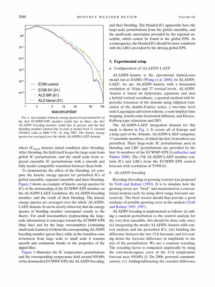
To demonstrate the effect of the blending, we com-

pute the kinetic energy spectra for perturbed ICs of

global ensemble, regional ensemble and their blending.

Figure 2 shows an example of kinetic energy spectra for

ICs of the downscaling of the ECMWF-EPS member on

the ALADIN-LAEF resolution, the ALADIN-breeding

member, and the result of their blending. The kinetic

energy spectra are averaged over the whole ALADIN-

LAEFdomain. It can be clearly observed, that the energy

spectra of blending member correspond exactly to the

theory. For small wavenumbers (representing the large-

scale information) it converges toward the ECMWF-EPS

(blue line) and for the large wavenumbers (containing

small-scale features) it follows the correspondingALADIN

breeding member (green line), while in the transition zone

in-between from large scale to small scale it remains

smooth and continuous thanks to the properties of the

digital filter.

Figure 3 illustrates the IC temperature perturbations

and the corresponding temperature field around 850hPa

of the downscaledECMWF-EPS, theALADINbreeding,

and their blending. The blended ICs apparently have the

large-scale perturbations from the global ensemble, and

the small-scale uncertainty provided by the regional en-

semble, which cannot be found in the global EPS. As

a consequence, the blended ICs should bemore consistent

with the LBCs provided by the driving global EPS.

3. Experimental setup

a. Configuration of ALADIN-LAEF

ALADIN-Austria is the operational limited-area

model run at ZAMG (Wang et al. 2006). In ALADIN-

LAEF, we use ALADIN-Austria with a horizontal

resolution of 18 km and 37 vertical levels. ALADIN-

Austria is based on hydrostatic equations and uses

a hybrid vertical coordinate, a spectral method with bi-

periodic extension of the domain using elliptical trun-

cation of the double-Fourier series, a two-time level

semi-Lagrangian advection scheme, a semi-implicit time

stepping, fourth-order horizontal diffusion, and Davies–

Kalberg-type relaxation and DFI.

The ALADIN-LAEF integration domain for this

study is shown in Fig. 4. It covers all of Europe and

a large part of the Atlantic. ALADIN-LAEF comprises

17 ensemble members, of which the first 16 members are

perturbed. Their large-scale IC perturbations used in

blending and LBC perturbations are provided by the

first 16 members of the ECWMF-EPS (Leutbecher and

Palmer 2008). The 17th ALADIN-LAEF member con-

tains ICs and LBCs from the ECMWF-EPS control

forecast with resolution of T399L62.

b. ALADIN breeding

Breeding (breeding of growing vectors) was proposed

by Toth and Kalnay (1993). It is to simulate how the

growing errors are ‘‘bred’’ and maintained in a conven-

tional analysis cycle by using short-range forecasts suc-

cessively. The bred vectors should thus provide a good

estimate of possible growing error in the analysis (Toth

and Kalnay 1993, 1997).

ALADIN breeding is implemented as follows: (i) add-

ing a random perturbation to the control analysis for

the very first ensemble, this should be done only once;

(ii) integrating the model ALADIN-Austria with con-

trol analysis and the perturbed ICs; (iii) building the

difference between the two 12-h forecasts; and (iv) scal-

ing down the forecast difference in amplitude to the

size of the perturbation. We use a constant rescaling.

The rescaling factor is computed empirically by using

the root-mean-square error of the 12-h temperature

forecast near 850 hPa (J. Du 2006, personal communi-

cation). (v) Adding/subtracting the rescaled difference

FIG. 2. An example of kinetic energy spectra for perturbed ICs of

the first ECMWF-EPS member (solid line in blue), the first

ALADIN breeding member (solid line in green), and the first

blending member (dotted line in red) at model level 31 (around

250 hPa) valid at 0000 UTC 10 Aug 2007. The kinetic energy

spectra are averaged over the whole ALADIN-LAEF domain.


to the new control analysis. The perturbed ICs are

generated in sets of positive and negative pairs around

the control analysis. Steps (ii) to (v) are then repeated,

and the perturbations are bred to grow along the fore-

cast trajectory. After a few cycles, the breeding vector

structure should be statistically independent of the very

first arbitrary perturbations (Magnusson et al. 2008). In

ALADIN breeding, wind components, temperature,

moisture, and surface pressure are perturbed at each

level and model grid point.

c. Experiments

To evaluate the blending, comparisons with dy-

namical downscaling of ECMWF-EPS and ALADIN

breeding have been conducted. In Table 1 the setup of

the comparison is described. In the experiment, we did

not apply any other perturbations, for example, the land

surface perturbation and the multiphysics for the model

perturbation in ALADIN-LAEF. This makes possible to

have a clean comparison between blending, dynamical

downscaling and breeding.

In our experiments, the resolution of ECMWF-EPS is

TL399L62 (spectral triangular T399 with 62 vertical

levels, corresponding to 50-km resolution). Initial con-

ditions are perturbed using a combination of initial time

and evolved singular vectors (Buizza and Palmer 1995)

computed at T42L62 resolution, with a 48-h optimiza-

tion time interval and a total-energy norm. Singular

vectors are computed to maximize the final-time norm

over different areas (Barkmeuer et al. 1999), then

FIG. 3. (left) IC perturbations of temperature at about 850 hPa and (right) the corresponding temperature fields.

(top) ALADIN breeding, (middle) downscaling of ECMWF-EPS, and (bottom) blending of ECMWF-EPS and

ALADIN-breeding. Valid at 0000 UTC 10 Aug 2007.


combined and scaled to have an initial amplitude

comparable to an estimate of the analysis error. Model

uncertainties due to physical parameterizations are

simulated using a stochastic scheme (Buizza et al.

1999). The ensemble control analysis is obtained by

interpolating the TL799L91 analysis to the ensemble

TL399L62 resolution.

For all those three experiments, the LBC perturba-

tions are provided by ECMWF-EPS forecasts in a 6-h

interval.

The blending implementation in this study is prac-

tically a breeding-blending cycle. Based upon the

ALADIN-LAEF 12-h forecasts, ALADIN breeding is

used to generate the IC perturbations, which are then

blended with the corresponding 16 perturbed ICs of

ECMWF-EPS. The new blended IC perturbations for

each of the 16 ALADIN-LAEF members are used as

ICs for the ALADIN-LAEF forecast; the ALADIN-

LAEF 12-h forecasts are employed for the next

breeding-blending cycle. In short, the blending system

takes its small scales from a separate breeding cycle

based on the ALADIN-LAEF 12-h forecasts started

with the blended IC perturbations.

In our implementation of blending, the spectral res-

olution of ECMWF ensemble TfG is equal to 399; and

the spectral resolution of its IC perturbations (i.e.,

the resolution of ECMWF SV TpG 5 42); the ECMWF

equivalent spectral resolution for ALADIN-LAEF TfR

is L/(3 3 18 km) 5 741, where L 5 40 000 km is the

Earth’s perimeter and 3 represents the denominator for

ALADIN-LAEF quadratic grid. Therefore, the blending

spectral truncation is computed as

TaG 5

ffiffiffiffiffiffiffiffiffiffiffiffiffiffiffiffiffiffiffiTfG 3T

pG

qffi 129; Tcut

R 5ffiffiffiffiffiffiffiffiffiffiffiffiffiffiffiffiffiffiffiffiTa2G 3T

fR

3

qffi 231,

and the blending ratioTfR/T

cutR is about 3.2. InALADIN-

LAEF the original spectral resolution, the maximum

zonal and meridional wavenumbers are 107 and 74,

the corresponding blending spectral truncation imple-

mented in this study are then 33 and 23, respectively. In

the implementation of DFI, we used the standard

Dolph–Chebyshev filter. The DFI is applied by in-

tegrating ALADIN backward adiabatically and forward

diabatically. The time span of the filter is 4 h with eight

integration time steps in each direction.

4. Results

In this study the ALADIN-LAEF runs with blend-

ing, breeding, and dynamical downscaling have been

initialized at 0000 UTC and integrated to 54 h for

a 2-month period (15 June–20 August 2007). The fore-

casts of upper-air weather variables were verified against

ECMWF analysis, and both analysis and forecast are

interpolated to a common regular 0.158 3 0.158 latitude–longitude grid. Verification of the forecasts of surface

weather variables were performed against the surface

observations at the observation location. Forecast values

are interpolated to the observation site for smoothly

varying fields, such as 2-m temperature and 10-m wind

speed. For precipitation, which has strong spatial gradi-

ents, the observation is matched to the nearest grid point.

The verification is performed for a limited area of the

forecast domain over central Europe, as shown in Fig. 4.

There are 1219 synop stations in the verification domain

being used in this study.

A set of standard ensemble and probabilistic forecast

verification scores is applied to evaluate the perfor-

mance of the ALADIN-LAEF experiments. The scores

considered are ensemble spread, root-mean-square er-

ror (RMSE) of ensemble mean, continuous ranked

FIG. 4. ALADIN-LAEF domain and model topography. The

inner limited-area domain in red depicts the verification domain,

which covers all of central Europe.

TABLE 1. Description of experiments ‘‘downscaling,’’ ‘‘breed-

ing,’’ and ‘‘blending’’ used to evaluate the blending method.

ALADIN-LAEF is configured with initial perturbations generated

by using downscaling, breeding, and blending. The same lateral

boundary perturbations from the ECMWF-EPS forecast and the

same land surface analysis from ECMWF-EPS control are ap-

plied in those experiments. No multiphysics are in use in the

experiments.

Expt

Initial condition

perturbations

Lateral boundary

condition

perturbations

Downscaling Downscaling of

ECMWF-EPS

ECMWF-EPS forecast

Breeding ALADIN-breeding ECMWF-EPS forecast

Blending Blending ECMWF-EPS

with ALADIN-breeding

ECMWF-EPS forecast


probability score (CRPS), and outlier statistics. Those

verification scores measure the quality of probabilistic

forecasts of scalar quantities. A detailed description of

those verification scores can be found in Hamill and

Colucci (1997), Mason (1982), Jolliffe and Stephenson

(2003), Stanski et al. (1989), and Wilks (2006).

In this study, we focus on verification of the most con-

cerned variables in regional EPS: 2-m temperature (T2m),

10-m wind speed (W10m), 12-h accumulated rainfall

(PREC), and three representative upper-air variables:

temperature at 850hPa (T850), wind speed at 850hPa

(V850), and relative humidity at 850hPa (RH850).

a. Ensemble mean RMSE and spread

RMSE of the ensemble mean describes the de-

terministic skill of the ensemble and gives good mea-

sures of overall forecast performance. The ensemble

spread is the standard deviation of the ensemble mem-

bers with respect to its mean. It reflects the diversity of

the ensemble forecast. The RMSE should basically

match the spread if the ensemble is correctly predicting

the distribution of potential outcomes.

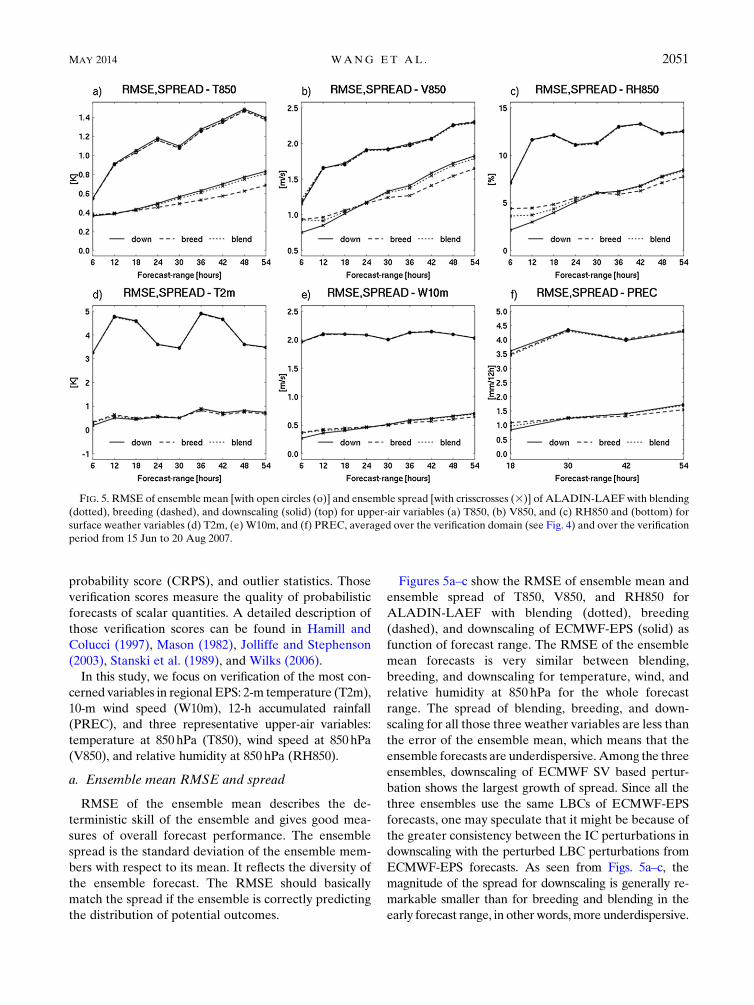
Figures 5a–c show the RMSE of ensemble mean and

ensemble spread of T850, V850, and RH850 for

ALADIN-LAEF with blending (dotted), breeding

(dashed), and downscaling of ECMWF-EPS (solid) as

function of forecast range. The RMSE of the ensemble

mean forecasts is very similar between blending,

breeding, and downscaling for temperature, wind, and

relative humidity at 850 hPa for the whole forecast

range. The spread of blending, breeding, and down-

scaling for all those three weather variables are less than

the error of the ensemble mean, which means that the

ensemble forecasts are underdispersive.Among the three

ensembles, downscaling of ECMWF SV based pertur-

bation shows the largest growth of spread. Since all the

three ensembles use the same LBCs of ECMWF-EPS

forecasts, one may speculate that it might be because of

the greater consistency between the IC perturbations in

downscaling with the perturbed LBC perturbations from

ECMWF-EPS forecasts. As seen from Figs. 5a–c, the

magnitude of the spread for downscaling is generally re-

markable smaller than for breeding and blending in the

early forecast range, in otherwords,more underdispersive.

FIG. 5. RMSE of ensemble mean [with open circles (o)] and ensemble spread [with crisscrosses (3)] of ALADIN-LAEF with blending

(dotted), breeding (dashed), and downscaling (solid) (top) for upper-air variables (a) T850, (b) V850, and (c) RH850 and (bottom) for

surface weather variables (d) T2m, (e) W10m, and (f) PREC, averaged over the verification domain (see Fig. 4) and over the verification

period from 15 Jun to 20 Aug 2007.


Very probably this is related to the lack of small scales in

the downscaled ECMWF initial perturbations.

The spread for breeding performs similar to blending

and downscaling in the early forecast range (up to 18 h)

for T850, but in the later forecast range the spread for

breeding grows clearly slower than for blending and

downscaling, in which the spread of blending and

downscaling keeps growing almost equally. For V850

and RH850 breeding has much larger spread than

downscaling up to 24–30 forecast hours. In the later

forecast range the spread of breeding grows slower and

becomes smaller than downscaling and blending.

As expected, blending has the best overall perfor-

mance. It takes the advantage of breeding and down-

scaling. In the early forecast range, the spread for

blending is similar (T850 and V850) or very closed

(RH850) to breeding, which is considerably better than

downscaling. This competitive performance of blending

shows the dominated effect of breeding in the blending

perturbation. During the later forecast range the spread

of blending keeps increasing rapidly as the downscaling,

which is superior to breeding. This might explain that

the blending of large-scale uncertainty from its driving

global model in regional IC perturbations makes it more

consistent with the LBC perturbations coming from the

driving global EPS.

The performance of blending, breeding, and down-

scaling for the surface weather variables has been also

compared in Figs. 5d–f, which show the RMSE of the

ensemble mean and the ensemble spread of T2m,

W10m, and PREC for ALADIN-LAEF with blending,

breeding, and downscaling. The RMSE of blending,

breeding, and downscaling performs very similar for

T2m andW10m; a slightly better RMSE of blending and

breeding than downscaling can be observed for PREC in

the early forecast hours (up to 30 h), then they reach the

RMSE of downscaling and give the same result in the

late forecast hours (30–54 h).

Like the upper-air variables, the spread of all the

surface weather variables, T2m, W10m, and PREC for

blending, breeding, and downscaling are remarkably

underdispersive. The positive impact of blending can

also be seen in the growth of ensemble spread for the

surface variables. Blending is close to breeding, which

performs better than downscaling in the first 24 forecast

hours. In the late forecast period downscaling is supe-

rior; this could be due to the matched IC perturba-

tions of downscaling with the LBC perturbations from

ECMWF-EPS forecasts. Blending is similar to down-

scaling, as it has the same large-scale perturbations as in

downscaling, which are more consistent with the LBC

perturbations from ECMWF-EPS forecasts. Breeding

has a larger spread in the early forecast range, but the

growth of spread is slower than blending and down-

scaling.

b. Outlier statistics

The measure of the statistical reliability discussed in

this subsection is the percentage of outliers. This is the

statistic of the number of cases when the verifying

analysis at any grid point lies outside the whole ensem-

ble. A more reliable EPS should have a score closer to

2/(nens 1 1), where nens is the ensemble size.

Figures 6a–c give the outlier statistics for the forecasts

of temperature, wind speed, and relative humidity at

850 hPa for blending, breeding, and downscaling; while

Figs. 6d–f show the outlier statistics for the forecasts of 2-m

temperature, 10-m wind speed, and 12-h accumulated

precipitation.

The benefit of using blending can be found in the

outlier statistics for both upper-air and surface weather

variables. For T850 and V850 in Figs. 6a and 6b, blending

gets the best reliability in terms of outlier statistics. Su-

perior results for blending can be found for W10m and

PREC in Figs. 6d and 6f. Blending is close to breeding for

RH850 in Fig. 6c and for T2m in Fig. 6d at a short lead

time, they have less outliers than downscaling; and it

turns too close to downscaling at the later time, and they

have less outliers than breeding.

The result of outlier statistics and the result of the

ensemble spread in Fig. 5 are consistent with each other

for blending, breeding, and downscaling.

c. The continuous ranked probability score

The CRPS is an overall measure of the skill of

a probabilistic forecast, measuring the skill of the en-

semble mean forecast as well as the ability of the per-

turbations to capture the deviations around it (Bowler

and Mylne 2009). CRPS is the generalized form of the

discrete ranked probability score, simulating the mean

over all possible thresholds. As noted by Hersbach

(2000), CRPS is analogous to an integrated form of the

Brier score, which can be decomposed into reliability,

resolution, and uncertainty. The CRPS orientates neg-

atively, so smaller values are better; and it rewards

concentration of probability around the step function

located at the observed value. A perfect CRPS score is

zero, as with the Brier score (Wilks 2006).

Figure 7 shows CRPSs of upper-air variables T850,

V850, and RH850 for blending, breeding, and down-

scaling; and of surface variables T2m,W10m, and PREC,

respectively. The statistical significant tests for CRPS are

computed by using the bootstrap method (Wilks 2006).

The 95% and 5% confidence intervals for the three ex-

periments and all the verifying upper-air and surface

variables are also shown in Fig. 7. The differences in the


skill score are statistically not significant, but noticeable.

CRPS score supports the findingswith spread and outliers

in the previous subsections. The blending has the best

performance, while breeding is better only at the short

lead time.

d. A case study

The impact of blending is evaluated by using several

standard statistical scores over a 2-month period in the

last subsections. To better understand the blending

method and its outperformance over the downscaling

and the regional breeding, a case study is investigated.

Figure 8 shows the time evolution of ensemble spread

of T850 of ALADIN-LAEF with the blending, the

breeding and the downscaling from initial time to 48-h

forecasts in a 12-h interval. The ensemble spread was

calculated on each grid over the whole ALADIN-LAEF

domain. It is a widely used measure to describe the

perturbation in the ensemble forecast. The blending has

more local small-scale information than downscaling at

initial time as expected; these scales cannot be properly

resolved by the downscaling. The ensemble spread of

blending has a similar distribution to the breeding, but

is smaller. The blending spread grows faster than the

breeding and becomes close to downscaling in the later

forecast range. The larger spread in the breeding at

initial time keeps the same magnitude and does not

grow during the forecast hours. It is noted that the local

small-scale perturbation in the blending and the

breeding decays after 12 forecast hours. The difference

of perturbations in the blending and the breeding at the

large scale keeps visible in the earlier and later forecast

range. These results are consistent with the result of

the 2 months of statistical scores discussed previously.

The ensemble spread of surface pressure has been

also investigated. They show the similar results (not

shown).

Figure 9 shows the time evolution of kinetic energy

spectra for perturbed ICs and forecasts of theALADIN-

LAEF member with downscaling, breeding, and blend-

ing at around 700 hPa. The kinetic energy spectra are

averaged over the whole ALADIN-LAEF domain.

Such a spectral analysis at different lead times for this

selected case can help us to understand ‘‘how’’ different

FIG. 6. Percentage of outliers of ALADIN-LAEF with blending (dotted), breeding (dashed), and downscaling (solid) (top) for upper-

air variables (a) T850, (b) V850, and (c) RH850 and (bottom) for surface weather variables (d) T2m, (e) W10m, and (f) PREC. The

verification domain and period are as in Fig. 5. The constant line in gray is the expected ideal percentage of outliers.


perturbations evolve with time and, therefore, help to

explain their forecast skills.

The effect of the blending is obviously at the initial

time and in the earlier forecast range. After 12–18-h

forecasts the kinetic energy spectra of blending, breed-

ing, and downscaling at the small scale get closer to each

other. The spectra of the blending remains the same as

downscaling, while the spectra of the breeding differs

from the blending and downscaling at large scale clearly

in the earlier forecast range, and still keeps visible in the

later forecast range. This confirms the results discussed

before.

5. Summary and conclusions

In this paper a new blending method for generating

IC perturbations in regional EPS has been proposed

and described. Blending combines the large-scale IC

perturbations from the global EPS with the small-scale

IC perturbations from the regional EPS by using

the digital filter and spectral analysis techniques. The

blending method is implemented in ALADIN-LAEF,

in which the large-scale IC perturbations are provided by

ECMWF-EPS, and the small-scale IC perturbations are

generated by breeding in ALADIN-LAEF. Ensemble

forecasts with blending are compared with ensembles

with regional breeding and dynamical downscaling of

ECMWF-EPS. Results are evaluated by using some

standard verification scores over central Europe and for

a 2-month summer period in 2007. A case study is also

conducted to have an in-depth analysis of the results. We

verified the surface weather variables: 2-m temperature,

10-mwind, and 12-h accumulated rainfall; and the upper-

air weather variables: wind, temperature, and relative

humidity at 850 hPa.

The IC perturbations generated by blending imple-

mented in ALADIN-LAEF can provide a better esti-

mate of the actual errors in the initial analysis based on

the past information about the flow through breeding.

The small-scale uncertainty in the analysis is more de-

tailed and accurate due to the higher resolution of

ALADIN, and it is more in balance with the orographic

FIG. 7. Comparison of (top) CRPSs of upper-air variables (a) T850, (b) V850, and (c) RH850 and (bottom) surface weather variables

(d) T2m, (e) W10m, and (f) PREC between ALADIN-LAEF with blending (dotted), breeding (dashed), and downscaling (solid). The

verification domain and period are as in Fig. 5. The faint lines of solid, dashed, and dotted show the 95% and 5% confidence intervals of

downscaling, breeding, and blending experiments, respectively.


FIG. 8. Ensemble spread of T850 of ALADIN-LAEF with blending (blend), breeding

(breed), and downscaling (down) from initial time to 48-h forecasts in a 12-h interval. The

forecast started at 1200 UTC 23 May 2011.


and surface forcing that is used in the regional model.

This is a better representation of reality than the in-

terpolated large-scale perturbations from the global

model, for example, through dynamical downscaling,

since these scales are not resolved in the global model.

On the large scale, the regional IC perturbations gen-

erated by blending are the uncertainties from ECMWF-

EPS, which can better sample the large-scale feature

FIG. 9. Kinetic energy spectra for perturbed ICs and forecasts of first member of

ALADIN-LAEF with downscaling (down, solid line in blue), breeding (breed, solid line

in green), and blending (blend, dashed line in red) at model level 20 (around 700 hPa).

The kinetic energy spectra are averaged over the whole ALADIN-LAEF domain. The

forecast started at 1200 UTC 23 May 2011.


because of its global geographical extent. As the LBC

perturbations are provided by ECMWF-EPS forecasts,

the IC perturbations of blending on the larger scale are

now consistent with the LBC perturbations.

Those features in the IC perturbations of blending

have been confirmed by the experiments presented in

this study, and it leads to the conclusion that blending

has the best overall performance in comparison with

breeding and downscaling.

The RMSE of the ensemble mean for blending,

breeding, and downscaling is very close to each other.

All three ensembles are underdispersive; their spread is

less than the errors of their ensemble mean, this is even

more evident for the surface variables. One may spec-

ulate that the strong underdispersion for the surface

weather variables may be due to lack of the perturba-

tions in the model physics and land surface conditions. It

should be also noted that the little spread might be due

to some extent to observation error (including the error

of representativeness, which may be particularly large

for station observations of surface variables) rather than

a deficiency in the ensemble (Saetra et al. 2004).

Downscaling underperforms at the short lead time.

The ensemble spread, statistical reliability, and the skill

score of CRPS for downscaling is noticeable inferior to

breeding and blending. Very probably this is related to

the lack of small scales in the downscaled ECMWF

initial perturbations. Downscaling of ECMWF SV-

based perturbation shows the largest growth rate of

spread among the three ensembles, and in the later

forecast period (after 24 h roughly) performs well, which

is comparable to blending. The relative rapid growth of

spread for downscaling might correspond to the greater

consistency between the IC perturbations in downscaling

with the LBC perturbations from the ECMWF-EPS

forecast, since all three ensembles use the same per-

turbed LBCs from ECMWF-EPS forecasts.

Breeding is superior during the first 24 forecast hours,

it has larger spread, which is better matched RMSE, has

fewer outliers, and slightly higher skill. A plausible ex-

planation for less underdispersion of breeding at the

short lead time may be due to the more detailed small-

scale IC perturbations generated by the regionalALADIN

breeding. In the later forecast range the spread of breeding

grows slower and becomes smaller than downscaling and

blending. This would be speculated to be due to the mis-

match between the IC perturbations generated by breed-

ingwith the large-scale forcing throughLBCperturbations

from ECMWF-EPS forecasts, and/or the properties of

breeding method itself (Wang and Bishop 2003). How-

ever, more in-depth studies are needed to verify if it is

really true or not. This is left to be our future research to

better understand the mechanism of blending.

One would expect that breeding performs better than

the downscaling, since it is attempting to simulate the

errors in the regional forecast. This would be true for the

short lead times since the IC perturbations are impor-

tant in this period; as the influence of the IC perturba-

tions decrease with increasing leading time, the impact

of the mismatch between IC and LBC perturbations be-

comes more dominant. This would suggest that regional

ensemble is best if it considers not only the uncertainties

in the regional analysis, but also the consistency between

the IC and LBC perturbations.

Blending has the best overall performance. In the

early forecast hours, blending is similar or much closer

to breeding, which is considerably better than down-

scaling. This competitive performance of blending shows

that the blending perturbations, like breeding, contain

more detail on the small scale than downscaling, which

persists to 24 h roughly. During the later forecast range

the spread of blending keeps increase rapidly as the

downscaling, which is superior to breeding. This is due to

the impact of the LBC perturbations. Blending has the

same large-scale perturbations as in downscaling, which

are consistent with the LBC perturbations.

As expected from the design of the blending method,

blending ensures that the scale of the IC perturbations

matches the scale resolved by the regional model, and

ensures that the IC perturbations match the LBC per-

turbations. It makes it possible that blending has the best

overall performance.

The case study confirms the results from the 2-month

averaged verification. It helps to better comprehend

how the blending works. The time evolution of the en-

semble spread and the kinetic energy spectra of the

blending, breeding, and downscaling prove that the ef-

fect of the blending is at the initial time and in the earlier

forecast range. The blending becomes close to the

downscaling at all the scales with the time, while the

breeding differs from the blending and downscaling at

the large scale clearly in the earlier forecast range, and

keeps visible in the later forecast range.

It has been noted that there are some issues that are

not investigated in this study, for example, what signal in

IC perturbations generated by breeding and downscal-

ing is good for the error growth in the ensemble, why

does the mismatch between IC and LBC cause the

slower growth rate of spread in the ensemble in the later

forecast hours, and what is the effect of spinup process

on IC perturbations for blending, breeding, and down-

scaling? These questions will be addressed in future

studies to better understand the mechanism of the

blending.

Furthermore, we are going to apply the blending idea

in convection-allowing ensembles. For such an ensemble,


it would need to have its own initial perturbations, which

represent the uncertainties in the corresponding reso-

lution. Further, because the model domain of such an

ensemble is usually rather small, the possible impact of

the LBC perturbations and the mismatch between IC

and LBC perturbations might bemore significant. These

possibilities will be investigated in the future, too.

Acknowledgments. We gratefully acknowledge Domi-

nique Giard, Radmila Brozkova, and Dijana Klaric who

have contributed to the ALADIN spectral blending.

Special thanks to Jun Du, Craig Bishop, Xuguang Wang,

and Zoltan Toth for valuable discussions during the

ALADIN-LAEF implementation. ECMWF has pro-

vided the computer facilities and technical help imple-

menting ALADIN-LAEF on the ECMWF HPCF. The

work has been partly funded by RC LACE and €OAD

(Austrian Agency for International Cooperation in Ed-

ucation and Research, Project CN 13/2010).

REFERENCES

Barkmeuer, J., R. Buizza, and T. N. Palmer, 1999: 3D-Var Hessian

singular vectors and their potential use in the ECMWF en-

semble prediction system. Quart. J. Roy. Meteor. Soc., 125,

2333–2351, doi:10.1002/qj.49712555818.

Bishop, C. H., and Z. Toth, 1999: Ensemble transformation and

adaptive observations. J. Atmos. Sci., 56, 1748–1765, doi:10.1175/

1520-0469(1999)056,1748:ETAAO.2.0.CO;2.

——, B. Etherton, and S. Majumdar, 2001: Adaptive sampling

with ensemble transform Kalman filter. Part I: Theoretical

aspects. Mon. Wea. Rev., 129, 420–436, doi:10.1175/

1520-0493(2001)129,0420:ASWTET.2.0.CO;2.

——, T. R. Holt, J. Nachamkin, S. Chen, J. G. McLay, J. D. Doyle,

andW. T. Thompson, 2009: Regional ensemble forecasts using

the ensemble transform technique.Mon. Wea. Rev., 137, 288–

298, doi:10.1175/2008MWR2559.1.

Bowler, N. E., and K. R. Mylne, 2009: Ensemble transform Kalman

filter perturbation for a regional ensemble prediction system.

Quart. J. Roy. Meteor. Soc., 135, 757–766, doi:10.1002/qj.404.——, A. Arribas, K. R. Mylne, K. B. Robertson, and S. E. Beare,

2008: TheMOGREPS short-range ensemble prediction system.

Quart. J. Roy. Meteor. Soc., 134, 703–722, doi:10.1002/qj.234.

Bro�zkov�a, R., and Coauthors, 2001: DFI blending, an alternative

tool for preparation of the initial conditions for LAM. PWRP

Rep. 31 (CAS/JSC WGNE Rep.), WMO-TD-1064, 1–7.

——, M. Derkova, M. Bellus, and F. Farda, 2006: Atmospheric

forcing by ALADIN/MFSTEP and MFSTEP oriented tun-

ings. Ocean Sci., 2, 113–121, doi:10.5194/os-2-113-2006.

Buizza, R., and T. Palmer, 1995: The singular vector structure of the

atmospheric general circulation. J. Atmos. Sci., 52, 1434–1456,

doi:10.1175/1520-0469(1995)052,1434:TSVSOT.2.0.CO;2.

——,M. Miller, and T. N. Palmer, 1999: Stochastic representation of

model uncertainties in the ECMWF Ensemble Prediction Sys-

tem. Quart. J. Roy. Meteor. Soc., 125, 2887–2908, doi:10.1002/

qj.49712556006.

Caron, J. F., 2013: Mismatching perturbations at the lateral bound-

aries in limited-area ensemble forecasting: A case study. Mon.

Wea. Rev., 141, 356–374, doi:10.1175/MWR-D-12-00051.1.

Derkov�a, M., and M. Bellu�s, 2007: Various applications of the

blending by digital filter technique in ALADIN numerical

weather prediction system. Meteor. J. SHMU, 10, 27–36.Du, J., and M. S. Tracton, 2001: Implementation of a real-time

short-range ensemble forecasting system at NCEP: An

update. Preprints, Ninth Conf. on Mesoscale Processes,

Ft. Lauderdale, FL, Amer. Meteor. Soc., P4.9. [Available online

at https://ams.confex.com/ams/WAF-NWP-MESO/techprogram/

paper_23074.htm.]

——, G. DiMego, M. S. Tracton, and B. Zhou, 2003: NCEP short-

range ensemble forecasting (SREF) system: Multi-IC, multi-

model and multi-physics approach. Research Activities in

Atmospheric andOceanicModeling,Rep. 33, CAS/JSCWorking

Group Numerical Experimentation (WGNE), WMO/TD-1161,

5.09–5.10.

Frogner, I. L., H. Haakenstad, and T. Iversen, 2006: Limited-

area ensemble predictions at the Norwegian Meteorological In-

stitute. Quart. J. Roy. Meteor. Soc., 132, 2785–2808, doi:10.1256/

qj.04.178.

Giard, D., 2001: Blending of initial fields in ALADIN. Internal

Documentation Note, GMAP/CNRM, Meteo-France, 28 pp.

[Available online at http://www.cnrm.meteo.fr/gmapdoc/

IMG/ps/Blending.aw-3.ps.]

Grimit, E. P., and C. F. Mass, 2002: Initial results of a mesoscale

short-range ensemble forecasting system over the Pacific

Northwest. Wea. Forecasting, 17, 192–205, doi:10.1175/

1520-0434(2002)017,0192:IROAMS.2.0.CO;2.

Hamill, T.M., and S. J. Colucci, 1997: Verification ofEta/RSM short-

range ensemble forecasts. Mon. Wea. Rev., 125, 1312–1327,

doi:10.1175/1520-0493(1997)125,1312:VOERSR.2.0.CO;2.

Hersbach, H., 2000: Decomposition of the continuous ranked

probability score for ensemble prediction systems. Wea. Fore-

casting, 15, 559–570, doi:10.1175/1520-0434(2000)015,0559:

DOTCRP.2.0.CO;2.

Iversen, T., A. Deckmyn, C. Santos, K. Sattler, J. B. Bremnes,

H. Feddersen, and I. L. Frogner, 2011: Evaluation of

‘GLAMEPS’—A proposed multimodel EPS for short

range forecasting. Tellus, 63A, 513–530, doi:10.1111/

j.1600-0870.2010.00507.x.

Jolliffe, I., and D. Stephenson, 2003: Forecast Verification: A

Practitioner’s Guide in Atmospheric Science. Wiley and Sons,

240 pp.

Leutbecher, M., and T. Palmer, 2008: Ensemble forecasting.

J. Comput. Phys., 227, 3515–3539, doi:10.1016/j.jcp.2007.02.014.Li, X., M. Charron, L. Spacek, and G. Candille, 2008: A regional

ensemble prediction system based on moist targeted singular

vectors and stochastic parameter perturbation. Mon. Wea.

Rev., 136, 443–462, doi:10.1175/2007MWR2109.1.

Lynch, P., and X. Huang, 1992: Initialization of the HIRLAM

model using a digital filter. Mon. Wea. Rev., 120, 1019–1034,

doi:10.1175/1520-0493(1992)120,1019:IOTHMU.2.0.CO;2.

——, D. Giard, and V. Ivanovici, 1997: Improving the efficiency of

a digital filtering scheme for diabatic initialization.Mon. Wea.

Rev., 125, 1976–1982, doi:10.1175/1520-0493(1997)125,1976:

ITEOAD.2.0.CO;2.

Machenhauer, B., and J. E. Haugen, 1987: Test of a spectral limited

area shallow water model with time dependent lateral bound-

ary conditions and combined normal mode/semi-Lagrangian

time integration schemes. Proc. ECMWF Workshop on

Techniques for Horizontal Discretization in Numerical Pre-

diction Models,Reading, United Kingdom, ECMWF, 361–377.

Magnusson, L., M. Leutbecher, and E. K€allen, 2008: Comparison

between singular vectors and breeding vectors as initial


https://ams.confex.com/ams/WAF-NWP-MESO/techprogram/paper_23074.htm

https://ams.confex.com/ams/WAF-NWP-MESO/techprogram/paper_23074.htm

http://www.cnrm.meteo.fr/gmapdoc/IMG/ps/Blending.aw-3.ps

http://www.cnrm.meteo.fr/gmapdoc/IMG/ps/Blending.aw-3.ps

perturbations for the ECMWF Ensemble Prediction System.

Mon. Wea. Rev., 136, 4092–4104, doi:10.1175/2008MWR2498.1.

Marsigli, C., A. Montani, and T. Paccagnella, 2008: A spatial verifi-

cation method applied to the evaluation of high-resolution

ensemble forecasts. Meteor. Appl., 15, 125–143, doi:10.1002/

met.65.

Mason, I., 1982: Amodel for assessment of weather forecasts.Aust.

Meteor. Mag., 30, 291–303.McMurdie, L., and C. F. Mass, 2004: Major numerical forecast

failures over the northeast Pacific. Wea. Forecasting,

19, 338–356, doi:10.1175/1520-0434(2004)019,0338:

MNFFOT.2.0.CO;2.

Saetra,O., H.Hersbach, J. Bidlot, andD.Richardson, 2004: Effects

of observation errors on the statistics for ensemble spread and

realiability. Mon. Wea. Rev., 132, 1487–1501, doi:10.1175/

1520-0493(2004)132,1487:EOOEOT.2.0.CO;2.

Stanski, H., L. Wilson, and W. Burrows, 1989: Survey of common

verification methods in meteorology. WMO/WWW Tech.

Rep. 8, 114 pp.

Stappers,R., and J. Barkmeijer, 2011: Properties of singular vectors

using convective available potential energy as final time norm.

Tellus, 63A, 373–384, doi:10.1111/j.1600-0870.2010.00501.x.

Stensrud, D. J., J. W. Bao, and T. T. Warner, 2000: Using initial

condition and model physics perturbations in short-range en-

semble simulations of mesoscale convective systems. Mon.

Wea. Rev., 128, 2077–2107, doi:10.1175/1520-0493(2000)128,2077:

UICAMP.2.0.CO;2.

Toth, Z., and E. Kalnay, 1993: Ensemble forecasting at NMC:

The generation of perturbation. Bull. Amer. Meteor. Soc.,

74, 2317–2330, doi:10.1175/1520-0477(1993)074,2317:

EFANTG.2.0.CO;2.

——, and ——, 1997: Ensemble forecasting at NCEP and the

breeding method. Mon. Wea. Rev., 125, 3297–3319,

doi:10.1175/1520-0493(1997)125,3297:EFANAT.2.0.CO;2.

Wang, X., and C. Bishop, 2003: A comparison of breeding and

ensemble Kalman filter ensemble forecast schemes. J. Atmos.

Sci., 60, 1140–1158, doi:10.1175/1520-0469(2003)060,1140:

ACOBAE.2.0.CO;2.

Wang, Y., T. Haiden, and A. Kann, 2006: The operational Limited

Area Modelling system at ZAMG: ALADIN-Austria.€Osterreich. Beitr. Meteor. Geophys., 37, 33 pp.

——, A. Kann, M. Bellus, J. Pailleux, and C. Wittmann, 2010: A

strategy for perturbing surface initial conditions in LAMEPS.

Atmos. Sci. Lett., 11, 108–113, doi:10.1002/asl.260.

——, and Coauthors, 2011: The Central European limited-area

ensemble forecasting system: ALADIN-LAEF.Quart. J. Roy.

Meteor. Soc., 137, 483–502, doi:10.1002/qj.751.

Warner, T., R. Peterson, and R. Treadon, 1997: A tutorial on

lateral boundary conditions as a basic and potentially se-

rious limitation to regional numerical weather predic-

tion. Bull. Amer. Meteor. Soc., 78, 2599–2617, doi:10.1175/

1520-0477(1997)078,2599:ATOLBC.2.0.CO;2.

Wei,M., Z. Toth, R.Wobus, andY. Zhu, 2008: Initial perturbations

based on the ensemble transform (ET) technique in the NCEP

global operational forecast system. Tellus, 60A, 62–79,

doi:10.1111/j.1600-0870.2007.00273.x.

Wilks, D. S., 2006: Statistical Methods in the Atmospheric Sciences.

2nd ed. Academic Press, 627 pp.

Zhang, F., C. Snyder, and R. Rotunno, 2002: Mesoscale predictability

of the ‘‘surprise’’ snowstorm of 24–25 January 2000. Mon. Wea.

Rev., 130, 1617–1632, doi:10.1175/1520-0493(2002)130,1617:

MPOTSS.2.0.CO;2.


a new method for generating initial condition ...cas.nuist.edu.cn/teacherfiles/file/20150916/... ·...

Documents