a new mineralogical approach to predict the …
TRANSCRIPT

A NEW MINERALOGICAL APPROACH TO PREDICT THE
COEFFICIENT OF THERMAL EXPANSION
OF AGGREGATE AND CONCRETE
A Thesis
by
SIDDHARTH NEEKHRA
Submitted to the Office of Graduate Studies of Texas A&M University
in partial fulfillment of the requirements for the degree of
MASTER OF SCIENCE
December 2004
Major Subject: Civil Engineering

ii
A NEW MINERALOGICAL APPROACH TO PREDICT THE
COEFFICIENT OF THERMAL EXPANSION
OF AGGREGATE AND CONCRETE
A Thesis
by
SIDDHARTH NEEKHRA
Submitted to the Texas A&M University in partial fulfillment of the requirements
for the degree of
MASTER OF SCIENCE
Approved as to style and content by:
Dan G. Zollinger Robert L. Lytton (Chair of Committee) (Member) Charles W. Graham David V. Rosowsky (Member) (Head of Department)
December 2004
Major Subject: Civil Engineering
iii
ABSTRACT
A New Mineralogical Approach to Predict the Coefficient of Thermal Expansion of
Aggregate and Concrete. (December 2004)
Siddharth Neekhra, B.E., Government Engineering College Raipur
Chair of Advisory Committee: Dr. Dan G. Zollinger
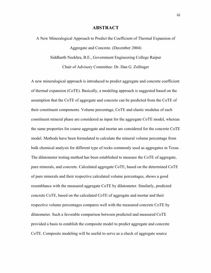
A new mineralogical approach is introduced to predict aggregate and concrete coefficient
of thermal expansion (CoTE). Basically, a modeling approach is suggested based on the
assumption that the CoTE of aggregate and concrete can be predicted from the CoTE of
their constituent components. Volume percentage, CoTE and elastic modulus of each
constituent mineral phase are considered as input for the aggregate CoTE model, whereas
the same properties for coarse aggregate and mortar are considered for the concrete CoTE
model. Methods have been formulated to calculate the mineral volume percentage from
bulk chemical analysis for different type of rocks commonly used as aggregates in Texas.
The dilatometer testing method has been established to measure the CoTE of aggregate,
pure minerals, and concrete. Calculated aggregate CoTE, based on the determined CoTE
of pure minerals and their respective calculated volume percentages, shows a good
resemblance with the measured aggregate CoTE by dilatometer. Similarly, predicted
concrete CoTE, based on the calculated CoTE of aggregate and mortar and their
respective volume percentages compares well with the measured concrete CoTE by
dilatometer. Such a favorable comparison between predicted and measured CoTE
provided a basis to establish the composite model to predict aggregate and concrete
CoTE. Composite modeling will be useful to serve as a check of aggregate source

iv
variability in terms of quality control measures and improved design and quality control
measures of concrete.

v
DEDICATION
This thesis is dedicated to my parents for their constant support, love and sacrifice.

vi
ACKNOWLEDGEMENTS
First, I would like to thank Dr. Dan G. Zollinger, without whose support and trust
I wouldn’t have been able to finish this work. I will never forget the good time I had
working with him. I can not find enough words to convey my gratitude towards him. I
would also like to thank Dr. Robert L. Lytton and Dr. Charles W. Graham for their time
and support as committee members.
I would like to thank Dr. Anal Mukhopadhyay for his valuable advice and
guidance during my research.
This research was sponsored by the Texas Department of Transportation. I would
like to gratefully acknowledge the financial support of TxDOT.
I would like to acknowledge the help of the Texas Transportation Institute (Texas
A&M University) lab staff especially Gerry Harrison for his help during the research.
Along with these people there were several others who were always with me just
in case I needed some help of any kind. This includes my friends at Texas A&M
University and back in India.
Finally, I would like to thank my family back at home. Their constant
encouragement, love and support kept me focused toward successful completion of this
thesis.

vii
TABLE OF CONTENTS Page
ABSTRACT ...................................................................................................................... iii
DEDICATION ....................................................................................................................v
ACKNOWLEDGEMENTS............................................................................................... vi
TABLE OF CONTENTS.................................................................................................. vii
LIST OF FIGURES .......................................................................................................... ix
LIST OF TABLES...............................................................................................................x
1. INTRODUCTION .........................................................................................................1
Objective ..................................................................................................................1 Role of Aggregate Coefficient of Thermal Expansion on CRC Pavement
Performance .......................................................................................................2 Method of Approach ................................................................................................4 2. LITERATURE REVIEW OF AGGREGATE AND CONCRETE CoTE ....................6
Aggregate Coefficient of Thermal Expansion .........................................................7 Chemical and Mineralogical Aspects of Aggregate CoTE................................8 Previous Methods of Testing for Aggregate and Concrete CoTE .........................10 Gnomix pvT High Pressure Dilatometer ...............................................................17 3. CoTE LABORATORY TESTING AND MODEL DEVELOPMENT........................18
Volumetric Dilatometer Method............................................................................18 Testing Apparatus and Calibration ........................................................................18 Testing Apparatus ............................................................................................18 Initial Total Volume...............................................................................22 Calibration of Apparatus........................................................................................23 The Coefficient of Thermal Expansion of Dilatometer ...................................23
The Coefficient of Thermal Expansion of Water ............................................23 Estimation of Errors.........................................................................................25
Verification of the Test Method.......................................................................27 Test for Steel and Glass Samples...........................................................27 Repeatability of the Dilatometer Tests in Measuring Aggregate CoTE..........29 Tests at Constant Temperature Conditions ......................................................32 Testing Protocol .....................................................................................................34 Preparing the Sample .......................................................................................34 Vacuuming.......................................................................................................35
viii
Page
Testing..............................................................................................................35 Analysis............................................................................................................35 4. MODELING APPROACH..........................................................................................36
Introduction............................................................................................................36 Modeling of Aggregate CoTE ...............................................................................37 Materials and Test Methods.............................................................................38 Determination of Mineral Weight Percentages from Bulk Chemical Analysis............................................................................................................40 Method I.................................................................................................41 Method II ...............................................................................................42 CoTE of Pure Minerals ...................................................................................45 Composite Modeling to Predict Aggregate CoTE...........................................45 Modeling of Concrete CoTE..................................................................................49 5. SUMMARY AND CONCLUSION ............................................................................52
Conclusion .............................................................................................................53 Quality Control Testing on the Aggregate CoTE ..................................................55 Quality Assurance Testing on Aggregate CoTE....................................................55 Specification Development....................................................................................56 Classification of Aggregate Based on Texture and CoTE.....................................57 REFERENCES ..................................................................................................................58
APPENDIX A....................................................................................................................60
APPENDIX B ....................................................................................................................63
APPENDIX C ....................................................................................................................65
APPENDIX D....................................................................................................................67
APPENDIX E ....................................................................................................................69
APPENDIX F.....................................................................................................................71
APPENDIX G....................................................................................................................73
VITA ................................................................................................................................74

ix
LIST OF FIGURES Page
Figure 1 Dilatometer Device............................................................................................ 5
Figure 2 Effect of CoTE of Slab Temperature on Crack Width (1). ............................... 8
Figure 3 Dilatometer Developed by Verbeck and Haas (16)......................................... 15
Figure 4 Concrete Specimen for Standard Test Method for the Coefficient of Thermal Expansion of Hydraulic Cement Concrete (17).............................................. 16
Figure 5 Gnomix pvT High Pressure Dilatometer (19). ............................................... 17
Figure 6 The Dilatometer Test Device.......................................................................... 19
Figure 7 Initial and Final Stages of Dilatometer Testing.............................................. 20
Figure 8 Thermal Expansion of Water.......................................................................... 25
Figure 9 Thermal Expansions of Steel Rod Samples Measured by Strain Gage.......... 29
Figure 10 Typical Data Measurements of Dilatometer Tests. ........................................ 30
Figure 11 Data Collections at a Constant Temperature (35°C). ..................................... 33
Figure 12 Composite Models for Concrete CoTE Calculation: (a) Parallel Model (b) Series Model (c) Hirsch’s Model. ............................................................. 39
Figure 13 Calculated vs Measured Aggregate CoTE. .................................................... 49
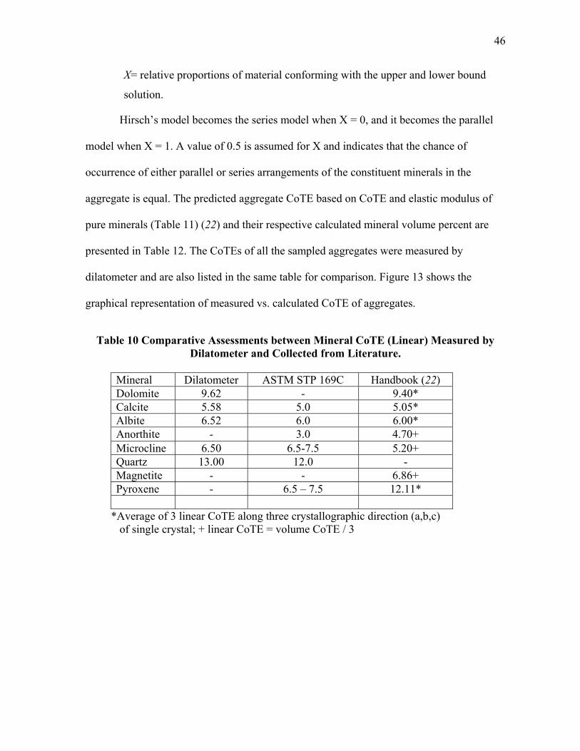
Figure 14 Calculated vs. Measured Concrete CoTE where X = 0.5 and MOE for Coarse Aggregate = 8 × 10⁶ psi. ..................................................................... 51
Figure 15 Schematic of Overall CoTE Implementation Strategy................................... 55

x
LIST OF TABLES Page
Table 1 Aggregate Properties........................................................................................... 6
Table 2 Aggregate CoTE Classification. ......................................................................... 8
Table 3 Densities of Water at Different Temperatures (20). ......................................... 24
Table 4 Possible Factors of Error and Their Significance. ............................................ 26
Table 5 Dilatometer Test Results for the Steel Rod Samples. ....................................... 28
Table 6 Comparison of CoTE of Glass Rods Obtained by Dilatometer and Strain Gage. ................................................................................................................. 31
Table 7 Comparison of Repeated CoTE Tests for Abilene Limestone. ........................ 31
Table 8 Bulk Chemical Analyses of the Tested Aggregates.......................................... 41
Table 9 Calculated Mineral Volume (Percent) by the Proposed Methods for the Tested Aggregates along with Actual Minerals Identified by XRD for Some Selected Aggregates.............................................................................. 44
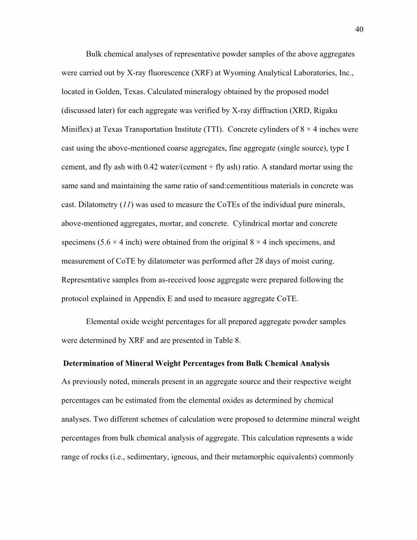
Table 10 Comparative Assessments between Mineral CoTE (Linear) Measured by
Dilatometer and Collected from Literature..................................................... 46 Table 11 CoTE of the Pure Minerals Measured by Dilatometer, Their Respective
Elastic Modulus and Phases Identified as Impurities by XRD. ...................... 47 Table 12 Mineral Volumes (percent) and Calculated CoTE for the Tested Aggregates
along with Measured CoTE by Dilatometer. .................................................. 47 Table 13 Mix Proportions of Concrete Specimens. ........................................................ 51
Table 14 Aggregate Classification System in Tα -N Format ........................................ 57

1
1. INTRODUCTION
OBJECTIVE
Aggregate properties play a very important role in the performance of continuously
reinforced concrete pavement (CRCP) pavements. In a continuously reinforced concrete
pavement, the key element to developing a uniform crack pattern is maintaining a balance
between the following aggregate factors that affect pavement performance:
• concrete, aggregate/paste early-age bond strength
• concrete drying shrinkage and creep
• aggregate coefficient of thermal expansion (CoTE)
• concrete strength
• modulus of elasticity, and
• aggregate type, gradation, and blend effects.
The present study focused on the role of aggregate CoTE. The coefficient of thermal
expansion is a length change in a unit length per degree (Celsius/Fahrenheit) temperature
change.
Most paving materials experience a change in volume due to a change in
temperature, and this dependency is described in terms of CoTE. Concrete is not an
exception to this and its CoTE depends on the thermal behavior of the individual
components (i.e., coarse aggregate, fine aggregate and cement paste). The type of coarse
and fine aggregate and the mixture proportion play an important role in the final CoTE of
the concrete (1).
This thesis follows the style of Transportation Research Board.

2
During the past decades several researchers have shown that the thermal properties of
cement, mortar, and aggregates can affect the thermal behavior of concrete (2). The CoTE
of the aggregate determines the thermal expansion of concrete to a considerable extent
because the aggregate composes of about 70-75 percent of the total solid volume of the
mixture. The aggregate also governs the degree of physical compatibility of the components
as the temperature changes (3).
Pavement distresses such as punchouts, faulting, corner breaks, and possibly
spalling are related to the thermal expansion properties of concrete (4). It has been
suggested that if the CoTE of the coarse aggregate and of the hydrated cement paste are
very different, a large change in temperature may introduce differential movement and thus
causing debonding (5). Therefore, characterization of key aggregate properties will enable
the projection of behavior of concrete with reasonable accuracy, which in turn may result in
improved understanding of pavement behavior and the effect of the material, thermal
spacing on performance.
Role of Aggregate Coefficient of Thermal Expansion on CRC Pavement Performance
The coefficient of thermal expansion of concrete is related to the volumetric change
hardened concrete undergoes as a result of temperature change. It certainly plays a role in
the thermal induced opening and closing of transverse cracks. The two main constituents of
concrete, cement paste and coarse aggregate (which have dissimilar thermal coefficients),
combine to form a composite coefficient of thermal expansion of concrete. Since more than
half of the concrete volume is coarse aggregate, the major factor influencing the coefficient
of thermal expansion of concrete appears to be the type of coarse aggregate. Studies
conducted by Brown (6) and later by Won et al. (7) showed that the effect of silica content

3
in the aggregate on the CoTE of the concrete is significant. This study indicated that the
higher the silica content, the higher the CoTE. Thermal effects are manifested in the daily
variation in the opening and closing of transverse cracks. This opening and closing
contributes to the stress in the reinforcing steel, but only to the extent that the CoTE of the
steel reinforcement is greater than the CoTE of the concrete. Consequently, the effect due to
the reinforcing steel stress is often much lower than the effect due to drying shrinkage.
However, the opening and closing of cracks is a factor in performance, since the degree of
load transfer is directly related to the width of the cracks. Therefore, crack widths should be
restricted within certain limits.
Several researchers have determined the coefficient of thermal expansion of various
aggregates and their results indicate that the coefficient of thermal expansion varies widely
among different aggregates, both with mineralogical content and with geographic location.
Some siliceous aggregates exhibit higher thermal expansion properties and have CoTE
values as high as 13 × 10-6/°C, whereas some limestone aggregates exhibit expansion values
lower than 6 × 10⁻⁶/°C (3, 5, 8, 9 ). Siliceous aggregates such as chert, quartzite, and
sandstone have CoTE that range between 10 × 10-6/°C to 12 × 10-6/°C, while basalt, granite,
and gneiss CoTE may vary between 6 × 10⁻⁶/°C to 9 × 10⁻⁶/°C. CoTE values for limestone
aggregates are typically less than granite or basalt. Measured CoTE values of granite range
between 8 × 10⁻⁶/°C to 9 × 10⁻⁶/°C, while the CoTE for basalt is typically slightly higher
than that of granite. The data have also demonstrated that aggregates of the same type and
from the same source may vary significantly in CoTE values.
CoTE characterization of an assorted mixture of aggregates will need improvement
in order to better understand the behavior patterns of concrete structures and concrete
4
pavements made with these different types of aggregates. It is anticipated that an estimated
value of the CoTE for concrete may be calculated from the weighted averages of the
coefficients of the aggregates and the hardened cement paste. Furthermore, the coarse
aggregate is expected to have the dominant effect upon the thermal expansion behavior of
concrete, as previously discussed. It has also been noted that concrete containing well-
graded aggregates has higher coefficient of thermal expansion values than concrete
containing gap-graded aggregates. The thermal behavior of the coarse aggregate may play a
greater role in the opening and closing of cracks after creep effects of concrete are
diminished due to aging and maturing of the concrete.
METHOD OF APPROACH
The available test data (5, 9) indicates that CoTE varies widely among different aggregates
with differing mineralogical content and geographical location. Since aggregates are
composite materials consisting of different minerals in different proportions, it is assumed
that their properties can be determined from the properties of their component minerals
(10). In this context, a new mineralogical approach to model aggregate CoTE, a composite
model to predict aggregate CoTE from the CoTE of constituent minerals and their
respective volume percentages is introduced. Similarly, concrete CoTE can be modeled
using the CoTE of constituent coarse aggregate and mortar. Validation of this composite
model can be established by drawing favorable comparisons between calculated and
measured CoTE. We use the volumetric dilatometer (11) to measure the CoTE of minerals,
aggregates and concrete in this context. The Volumetric dilatometer (Figure 1) is an
apparatus used to determine the bulk coefficient of thermal expansion of coarse aggregate,
fine aggregate and concrete.

5
Figure 1 Dilatometer Device.

6
2. LITERATURE REVIEW OF AGGREGATE AND CONCRETE CoTE
The role of physical, mechanical, and chemical properties of coarse aggregates on
the behavior and performance of paving concrete are often described in terms of their
effects on concrete strength, shrinkage, creep, and bond strength. Specific aggregate
properties are listed in Table 1 relative to their physical attributes. These physical attributes
can be related to concrete mixing, placing, finishing, hardening, and other construction and
pavement related characteristics. The mechanical properties of an aggregate predict its
ability to resist loads and stresses. The chemical properties of an aggregate are a result of its
chemical composition. Aggregate’s chemical interaction with concrete pore solution and
water depends on its chemical properties. CoTE is classified as mechanical property of
aggregate.
Table 1 Aggregate Properties.
Physical Mechanical Chemical Particle shape Strength Solubility Maximum particle size Elastic modulus Base exchange Surface texture Coefficient of thermal
expansion Surface charge
Percent voids Resilient modulus Chloride content Thermal conductivity Resistance to loads Reactivity Permeability Resistance to degradation Slaking Specific gravity Coatings Porosity Oxidation potential Gradation Resistivity

7
AGGREGATE COEFFICIENT OF THERMAL EXPANSION
As already mentioned earlier, aggregate CoTE is one of the most important behavioral
characteristics of an aggregate material, which is found to influence the performance of
concrete pavement primarily due to its effect on dimensional change under a change in
temperature. The CoTE of an aggregate has a marked effect on the CoTE of concrete
containing the given aggregate. Some of the pavement distresses are related to the thermal
expansion properties of jointed concrete (4), but the more pronounced effect is on the
development of the crack pattern and the daily and seasonal temperature changes on the
width of transverse cracks in CRC pavements, as it would affect their load transfer
efficiency.
Pavements are susceptible to bending and curling caused by temperature gradients that
develop when concrete is cool on one side and warm on the other (4). Moisture and
temperature variations cause volumetric changes that can lead to cracking and premature
failure in Portland cement Concrete (PCC) pavements. In jointed pavements, the volumetric
changes caused by friction between the concrete and the base can lead to transverse cracks
that can adversely affect load transfer and carrying capacity. Knowledge of this property
during the design stage of pavement before the construction allows for accurate prediction
of the potential thermal change on crack development and crack width and enhances the
overall design process. Siliceous gravel use results in larger crack width than does the
limestone and at low temperature of pavement this difference is higher (1) as shown in
Figure 2. These results provide an idea of how to classify aggregate based on their CoTE
values. Aggregate CoTE is divided into three categories (Table 2) based on their effects on
concrete performance.

8
Figure 2 Effect of CoTE of Slab Temperature on Crack Width (1).
Table 2 Aggregate CoTE Classification.
As previously discussed, the aggregate coefficient of thermal expansion is a
function of its mineralogical composition. This aspect is described below in detail.
Chemical and Mineralogical Aspects of Aggregate CoTE
Hardened concrete has a coefficient of thermal expansion greater than that of aggregate, but
the expansion of concrete is proportional to that of the aggregate, as aggregates form a
major part of the concrete (5). Aggregates commonly used in concrete are classified into
three major categories: igneous, sedimentary, and metamorphic rocks. These groups can be
further divided into subgroups depending on their chemical and mineral composition and
their textural and internal structure. Research suggests that a definable relationship exists
between the chemical and mineral composition of the aggregate and its measured CoTE. In
Category CoTE (10-6/°C)
Low <6
Medium 6-9
High >9
9
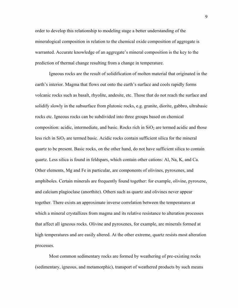
order to develop this relationship to modeling stage a better understanding of the
mineralogical composition in relation to the chemical oxide composition of aggregate is
warranted. Accurate knowledge of an aggregate’s mineral composition is the key to the
prediction of thermal change resulting from a change in temperature.
Igneous rocks are the result of solidification of molten material that originated in the
earth’s interior. Magma that flows out onto the earth’s surface and cools rapidly forms
volcanic rocks such as basalt, rhyolite, andesite, etc. Those that do not reach the surface and
solidify slowly in the subsurface from plutonic rocks, e.g. granite, diorite, gabbro, ultrabasic
rocks etc. Igneous rocks can be subdivided into three groups based on chemical
composition: acidic, intermediate, and basic. Rocks rich in SiO2 are termed acidic and those
less rich in SiO2 are termed basic. Acidic rocks contain sufficient silica for the mineral
quartz to be present. Basic rocks, on the other hand, do not have sufficient silica to contain
quartz. Less silica is found in feldspars, which contain other cations: Al, Na, K, and Ca.
Other elements, Mg and Fe in particular, are components of olivines, pyroxenes, and
amphiboles. Certain minerals are frequently found together: for example, olivine, pyroxene,
and calcium plagioclase (anorthite). Others such as quartz and olivines never appear
together. There exists an approximate inverse correlation between the temperatures at
which a mineral crystallizes from magma and its relative resistance to alteration processes
that affect all igneous rocks. Olivine and pyroxenes, for example, are minerals formed at
high temperatures and are easily altered. At the other extreme, quartz resists most alteration
processes.
Most common sedimentary rocks are formed by weathering of pre-existing rocks
(sedimentary, igneous, and metamorphic), transport of weathered products by such means

10
as wind and moving water, deposition of suspended materials from air or water,
compaction, and digenesis. Sedimentary rocks are also formed through chemical process
such as dissolution and precipitation of minerals in water and secretion of dissolved
minerals through organic agents.
Metamorphic rocks are formed by a process called metamorphism (i.e., during
burial or heating, where rocks experience recrystallization and mutual reaction of
constituent minerals as their stability fields are exceeded). Because these reactions take
place without ever reaching the silica melt phase, they are called metamorphic. After
formation, most rocks are exposed to a series of processes and cannot be classified by a
single process.
The variation of the CoTEs of the different types of aggregates can be explained by
the presence and proportions of different types of minerals they contain. It is true that
different rock types commonly used as aggregates have their characteristic chemical
compositions. Therefore, differences in chemical composition should ultimately reflect in
different mineralogy. The chemical composition will change if the rock types change.
Aggregate from the same source could have slightly different coefficients of thermal
expansion because of slight variations in mineralogy or textural features like
recrystallization, crystallinity, etc.
PREVIOUS METHODS OF TESTING FOR AGGREGATE AND CONCRETE
CoTE
Many attempts have been made to measure the coefficient of thermal expansion of
aggregates and concrete. Researchers have tried a number of different approaches, ranging
from using strain gages (to measure length change) to measurement of the volume change

11
of a collective sample. The majority of these test methods are based on the measurement of
linear expansion over a temperature range. However, determining the linear expansion of
fine aggregate is not possible because of the smaller size of particles. The method
explained by Willis and DeReus (12) allows measurements to be made over a considerable
particle size range using an optical lever. The specimens used by Willis and DeReus were
25.4 mm diameter cores, 50 mm long, drilled from the aggregate specimen to be tested and
placed in a controlled-temperature oil bath with a range of 2.78 ± 1.7°C to 60 ± 2.8°C .
When the temperature is varied the vertical movement of the specimen was measured by
observing through a precise level the image, reflected by mirror of optical lever, having
25.4 mm lever arm, on a vertical scale placed 6.1 m from the mirror. The calculated
coefficients of thermal expansion are probably accurate to ±3.6 × 10⁻⁶/°C by using the
method.
In the strain gage test method, developed by the U.S. Army Corps of Engineers (13),
electrical resistance wire strain gages measure the coefficient of thermal expansion of
coarse aggregate. The apparatus consists of
• a controlled-temperature cabinet,
• a SR-4 strain indicator,
• resistance electrical strain gages,
• suitable cement for attaching the gages to the specimens,
• a multipoint recording potentiometer,
• a standard specimen of known coefficient of thermal expansion,
• a switchboard with silver-contact switches in circuit with the SR-4 indicator,
• individual lead wires to the panel board,
12
• a panel board built for mounting specimens with gages attached through binding
posts to the lead wires,
• thermocouples for temperature measurements within a cabinet at various points, and
• a diamond cutoff wheel for sawing specimens.
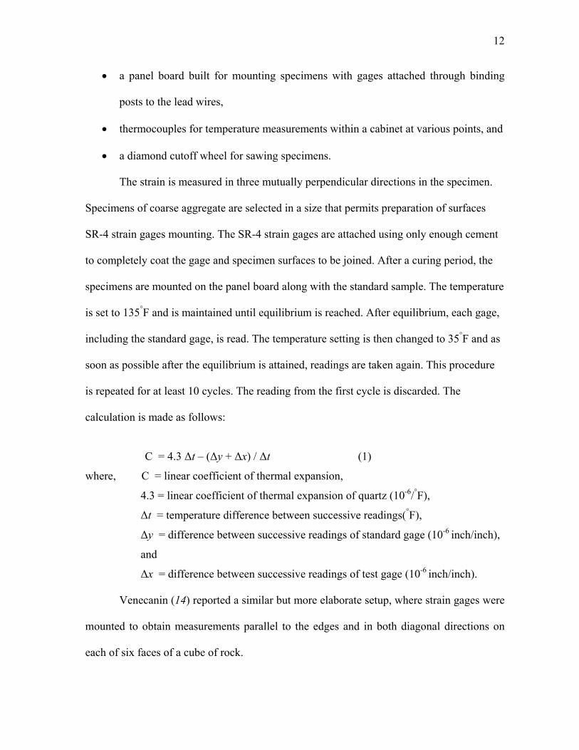
The strain is measured in three mutually perpendicular directions in the specimen.
Specimens of coarse aggregate are selected in a size that permits preparation of surfaces
SR-4 strain gages mounting. The SR-4 strain gages are attached using only enough cement
to completely coat the gage and specimen surfaces to be joined. After a curing period, the
specimens are mounted on the panel board along with the standard sample. The temperature
is set to 135°F and is maintained until equilibrium is reached. After equilibrium, each gage,
including the standard gage, is read. The temperature setting is then changed to 35°F and as
soon as possible after the equilibrium is attained, readings are taken again. This procedure
is repeated for at least 10 cycles. The reading from the first cycle is discarded. The
calculation is made as follows:
C = 4.3 ∆t – (∆y + ∆x) / ∆t (1)
where, C = linear coefficient of thermal expansion,
4.3 = linear coefficient of thermal expansion of quartz (10-6/°F),
∆t = temperature difference between successive readings(°F),
∆y = difference between successive readings of standard gage (10-6 inch/inch),
and
∆x = difference between successive readings of test gage (10-6 inch/inch).
Venecanin (14) reported a similar but more elaborate setup, where strain gages were
mounted to obtain measurements parallel to the edges and in both diagonal directions on
each of six faces of a cube of rock.

13
The main drawback of using strain gages is that they cannot be used on material
with different sizes and shapes. Creep of gages cemented to the surfaces can occur during
the test and cause errors in gage readings. Because of the size and usually heterogeneous
nature of fine aggregate, none of the preceding methods are readily adaptable to the
determination of the CoTE of this type of material. The usual approach has been to
determine the linear expansion of mortar bars containing the fine aggregate. However, the
results obtained include the effects of the length change contributed by the cement.
Mitchell (15) described a method in which specimens of 25.4 to 76.2 mm in size
were coated with wax and held in fulcrum-type extensometer frames. The specimens were
immersed in a circulating ethylene glycol solution held at a desired temperature, and
electromagnetic strain gages with electronic indicators were used for measurement.
The dilatometer method was devised in 1951 by Verbeck and Haas to measure the
coefficient of volumetric thermal expansion of aggregate (16). Their apparatus consisted of
a 1 Liter dilatometer flask to which was attached a laboratory-constructed capillary bulb
arrangement containing electrical contacts (Figure 3). In operation, the flask was filled with
aggregate and water then the apparatus was allowed to equilibrate at one of the controlling
electric contacts. The equilibrium temperature was measured with a Beckman thermometer.
Verbeck and Haas calculated the coefficient of thermal expansion on the basis of the
temperature required to produce an expansion equivalent to the volume between the
equilibrating electrical contacts. The apparatus needed to be calibrated to determine the
coefficient of volumetric thermal expansion of the flask. The aggregate sample was
immersed in water for a few days in order to remove any air present. The temperature
increment was approximately 4°C; however, this varied depending on the temperature at

14
which the flask was operated, the ratio of the volume increment between the contacts to the
flask volume, the amount of aggregate in the flask, and the thermal characteristics of the
aggregate. For measurements made below the freezing point of water, a non-reactive liquid,
such as toluene, which does not freeze at the desired temperature, could be substituted. It
was fairly easy to prepare the sample for the experiment. In comparison to other methods,
such as a mounted strain gage on a specific rock sample, this method has the advantage of
testing aggregates of different sizes.
A test method was recently developed by the American Association of State
Highway and Transportation Officials (AASHTO) as test number TP60-00, "Standard Test
Method for the Coefficient of Thermal Expansion of Hydraulic Cement Concrete"(17). The
procedure requires a 4 inch diameter core, cut to a length of 7 inches (Figure 4). The sample
is saturated for more than 48 hours and then subjected to a temperature change of 40°C in a
water bath. The length change of the specimen is measured and, with the known length
change of the measuring apparatus under the same temperature change, the CoTE of the
concrete specimen can be determined.

15
Figure 3 Dilatometer Developed by Verbeck and Haas (16)

16
Figure 4 Concrete Specimen for Standard Test Method for the Coefficient of Thermal Expansion of Hydraulic Cement Concrete (17).
A computer program, CHEM2 (18), was developed by the Center for Transportation
Research, The University of Texas at Austin, Texas, which allows the researcher to
estimate the properties of concrete compressive strength, coefficient of thermal expansion,
splitting tensile strength, elastic modulus, and drying shrinkage for curing times ranging
from 1 to 28 days using input of aggregate bulk chemical analysis results. The methodology
of the CHEM2 program is such that it first identifies the type of aggregate and then predicts
the performance using a model prepared for that type of aggregate. The program either
identifies the aggregate from either the user input or the bulk chemical analysis results.
CHEM2 is based on regression analysis of the oxide weight percentage of the
aggregate to predict concrete properties independent of concrete mixture proportions. This
program predicts mineral weight percent of all types of aggregates based on a common set
of chemical formulae.

17
GNOMIX PVT HIGH PRESSURE DILATOMETER (19)
Dilatometry measures the change in volume of a specimen subjected to different
temperatures and pressures. The Gnomix PVT Apparatus (Figure 5) generates pressure-
specific volume-temperature measurements using high-pressure dilatometry.
Approximately 1 gram of dry sample is loaded into a sample cell, and placed in the
PVT apparatus. The machine is brought to just below the melting point temperature,
Isothermal data acquisition begins as soon as the machine is brought at this temperature.
Volume readings are taken by an LVDT for the specified temperature at pressures ranging
from 10-200 MPa. The procedure is repeated for decreasing temperatures, down to ambient
temperature. Data may also be gathered while heating the specimen. From the gathered
data, the volumetric expansion coefficient in the solid state is extracted.
Figure 5 Gnomix pvT High Pressure Dilatometer (19).
18
3. CoTE LABORATORY TESTING AND MODEL DEVELOPMENT
VOLUMETRIC DILATOMETER METHOD
During the present study Volumetric Dilatometer (11) method was used to measure the
CoTE of both coarse and fine aggregate as well as pure minerals, metals, and glass.
Substantial modification in the design of the dilatometer was made in comparison with the
earlier version that Verbeck and Haas used, though the basic working principle remains the
same. The present data acquisition system is also entirely different than with Verbeck and
Hass’s model.
TESTING APPARATUS AND CALIBRATION
During this study a test apparatus referred to as a volumetric dilatometer for determining
the bulk coefficient of thermal expansion of both fine and coarse aggregates is used for
verification of model for aggregate and concrete coefficient of thermal expansion. The
method is particularly adaptable to the study of field-saturated coarse aggregates, sand and
concrete cores and provides a means of testing a representative sample of a heterogeneous
coarse aggregate.
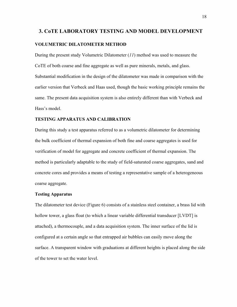
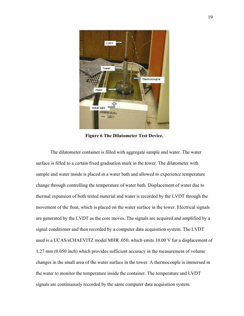
Testing Apparatus
The dilatometer test device (Figure 6) consists of a stainless steel container, a brass lid with
hollow tower, a glass float (to which a linear variable differential transducer [LVDT] is
attached), a thermocouple, and a data acquisition system. The inner surface of the lid is
configured at a certain angle so that entrapped air bubbles can easily move along the
surface. A transparent window with graduations at different heights is placed along the side
of the tower to set the water level.
19
Figure 6 The Dilatometer Test Device.
The dilatometer container is filled with aggregate sample and water. The water
surface is filled to a certain fixed graduation mark in the tower. The dilatometer with
sample and water inside is placed in a water bath and allowed to experience temperature
change through controlling the temperature of water bath. Displacement of water due to
thermal expansion of both tested material and water is recorded by the LVDT through the
movement of the float, which is placed on the water surface in the tower. Electrical signals
are generated by the LVDT as the core moves. The signals are acquired and amplified by a
signal conditioner and then recorded by a computer data acquisition system. The LVDT
used is a UCAS/sCHAEVITZ model MHR .050, which emits 10.00 V for a displacement of
1.27 mm (0.050 inch) which provides sufficient accuracy in the measurement of volume
changes in the small area of the water surface in the tower. A thermocouple is immersed in
the water to monitor the temperature inside the container. The temperature and LVDT
signals are continuously recorded by the same computer data acquisition system.

20
Dilatometer CoTE measurement is basically an estimation of the CoTE of the tested
material based on the volumetric relationships between water, tested material, and container
under a given temperature change. Research has shown that the linear CoTE of an isotopic
material is one-third the volumetric CoTE, (Appendix A) and for simplicity, the same is
assumed for all tested materials.
Figure 7 represents the initial and final states of a dilatometer test. The container is
filled with water and test sample so that the total initial and final volumes, V1 and V2,
consist of the volume of water, Vw, and volume of aggregate sample, Va, at each state. The
instrument test system measures the displacement of water level, ∆h, in the container tower
with the change of temperature. These measurements produce an estimation of the
coefficient of thermal expansion of aggregate sample based on the volumetric relationships
between water, aggregate, and container at a given temperature change.
Figure 7 Initial and Final Stages of Dilatometer Testing.
In operation, the container is placed in the water bath and heated by the water
surrounding it. When the temperature is raised from T1 to T2, the aggregate, the water, and

21
the container all expand. Therefore, the apparent volume change that the LVDT detects
consists of three parts:
∆V1 = A ∆h = ∆Va + ∆Vw - ∆Vf (2)
where ∆V1 = observed total volumetric increase due to temperature change ∆T,
A = inner sectional area of tower,
∆h = rise of the water surface inside the tower,
∆Vw = volumetric increase of water due to temperature ∆T,
∆Vf = volumetric increase of inside volume of the dilatometer due to ∆T,
∆Va = volumetric increase of aggregate Va due to ∆T, and
∆T = temperature increase from T1 to T2.
Since Vf = Va + Vw = V (3)
∆Va = Va γa ∆T
∆Vf = V γf ∆T
∆Vw = Vw γw ∆T = (V −Va) γw ∆T
where V = total inner volume of the flask,
Vw = volume of water in the flask,
Vf = volume of the flask,
Va = volume of aggregate in the flask,
γa = coefficient of volumetric thermal expansion of aggregate,
γw = coefficient of volumetric thermal expansion of water, and

22
γf = coefficient of volumetric thermal expansion of flask,
We have
+−−⋅−
∆∆⋅
= ))((1awfwwa
aa VVV
ThA
Vγγγγ (4)
The coefficient of thermal expansion of aggregate sample is calculated by equation
(4). Among the parameters on the right-hand side of the equation, the cross-sectional area
of the tower, A, is fixed known value for a dilatometer. The thermal coefficient of
container, γf, is also regarded as a fixed value. Other parameters, ∆h, ∆T, Vw, Va, and γw, are
variable and they are measured in the test or determined by applied test conditions. Close
review of the determination of the above input values will help clarify the validity of
equation (4).
Initial Total Volume
The initial total volume, V, consists of the volume of water and the volume of the
aggregate. This initial total volume is equivalent to the initial volume of the dilatometer, Vf.
The initial total volume, V or Vf, is determined by measuring the weight of the dilatometer
filled with water at a fixed level. The initial total volume is now determined by multiplying
the weight of water and the specific volume of water at the initial temperature (T1). The
weight of water is independent of temperature. Estimation of the specific volume of water
at different temperatures is described later in the section in the discussion of the coefficient
of thermal expansion of water.

23
CALIBRATION OF APPARATUS
The dilatometer is calibrated to separate the volumetric expansion of the water and the
container from the volumetric expansion of tested material.
The Coefficient of Thermal Expansion of the Dilatometer
The purpose of calibration of the dilatometer is to determine the apparent coefficient of
volumetric thermal expansion of the flask and to ensure that the variability from test to test
is within acceptable limits. The calibration procedure is described in Appendix B in the
form of a calibration protocol. The dilatometer is filled with distilled water and tested over
a temperature range from 100C to 500C in order to estimate the CoTE of the dilatometer
container. In this case, the volumetric relation shown in equation (4) becomes
TVhA
wf ∆⋅
∆⋅−=
1γγ (5)
where V = Vf = Vw and
Va = 0.
This calibration gives an apparent coefficient of thermal expansion of the
dilatometer of 55..33 ×× 1100--55 °C ±± 00..0044110011 over the temperature range used for the calibration,
the volumetric expansion of the dilatometer showed linear behavior; therefore, this value is
regarded as a constant.
The Coefficient of Thermal Expansion of Water
The volume change of water is known to be non linear with respect to temperature changes.
Therefore, the thermal coefficient of water, γw, is variable with respect to the selected
temperature for a test. This variable parameter γw can be determined from the density of
water at different temperatures (20) and is presented in Table 3.

24
Table 3 Densities of Water at Different Temperatures (20).
Temperature (°C)
Density (g/cm3)
Temperature (°C)
Density (g/cm3)
0 0.99984 60 0.98320 10 0.99970 70 0.97778 20 0.99821 80 0.97182 30 0.99565 90 0.96535 40 0.99222 100 0.95840 50 0.98803
The reciprocal of the density gives the specific volume of water at different
temperatures. The change in specific volume of water with temperature is shown in Figure
8. As shown in the Figure 8, the volumetric behavior of water under temperature change is
perfectly fitted with a fourth-order polynomial equation. The specific volume of water at
any given temperature from 0°C to 100°C can be estimated by the regression equation
shown in Figure 8. Now the volume change of water for any temperature change within the
range of 0°C to 100°C can be obtained as:
)(1)(1
121
12
1
12
TTvvv
TvWvvW
TVV
w −⋅−
=∆
⋅⋅
−⋅=
∆⋅
∆=γ (6)
where V = initial volume of water,
∆T = change of temperature from T1 to T2,
∆V = change of volume of water due to the temperature change,
W = weight of water,
v1 and v2 = specific volumes of water at temperatures T1 and T2, respectively.

25
Figure 8 Thermal Expansion of Water.
Estimation of Errors
Random or systematic errors may exist in the test protocol. Error and sensitivity are
evaluated with respect to the determination of input parameters and subsequent calculation
of the CoTE of aggregate.
In determining the initial volume, it is assumed that the water level is always at the
same position as long as the same graduation is used for the leveling. Precisely speaking,
however, even if the same graduation is used, the level of water may vary slightly within
the diameter due to the surface tension of the water. Consequent random error may exist in
determining the initial total volume. Presumably, however, the effect of this error is not
significant. The possible maximum error in CoTE caused by this random error in the water
leveling process is less than ±1.0 percent. Furthermore, the actual error in the positioning
the water would be much less than the maximum error level. Therefore, the possible
random error in positioning the initial water level can be regarded as negligible as long as
the same graduation is used for leveling the water.

26
Another random error may exist in determining the initial volume of aggregate
associated with the measurements of the weight of aggregate. The effect of error in weight
on the determination of volume is not significant. However, it should be recognized that the
initial volume of aggregate could influence the determination of the aggregate CoTE, as
previously noted. Considering that, in general, 3300 – 3700 g of saturated surface dry
aggregate is used for a normal CoTE test, it is expected that the maximum random error in
measuring the weight of aggregate would not be more than 5 g (0.125 percent). The thermal
coefficient of the dilatometer is assumed to be a constant as long as the shape, size, and
material of dilatometer remain same. If there is a difference between different dilatometers,
maximum error expected in the coefficient of thermal expansion of flask (γf) is 1 percent.
The sensitivity of the measurements on ∆h is greater than other parameters. Considering
that the general range of ∆h is determined to be 15 to 20 mm, an error of only a few tenths
of a millimeter produces significant error. This means the LVDT needs to be calibrated at
least to 1/100 mm, which is in the range of its precision. It should be recognized that the
thermal coefficient of water is much higher than the coefficient of the aggregate sample so
the majority of the volumetric expansion is governed by water. Table 4 presents a summary
of estimated factors of errors and their significance. Appendix C provides the details of
variance analysis done on these factors.
Table 4 Possible Factors of Error and Their Significance.
Type Factor Coefficient of Variation of
(a Positioning the initial water level -
Random Weight of aggregate 2.4 %
Thermal coefficient of dilatometer ((f)
1.2 % Systematic
Displacement reading ()h) 3.9 %

27
Verification of the Test Method
As previously noted, measurement errors associated with temperature change, float
displacement, and initial volume contribute to the error in determining the CoTE of
aggregate. In order to develop a procedure to reduce the calculated error, a series of
verification tests were conducted such as:
1. The test results from the dilatometer were compared with the results from strain
gage setups for samples (steel and glass) with known CoTE values.
2. The repeatability of the dilatometer tests with the same aggregate sample was
verified.
3. The data was tracked at a constant temperature condition to see if any systematic
problems exist in the dilatometer test setup.
Tests for Steel and Glass Samples
The validity of the dilatometer tests was examined by comparing CoTE values
obtained from the dilatometer with CoTE values from and different test schemes that use
strain-gaged specimens. Two different materials, steel rods and glass rods, were used in
these comparative tests. The steel and glass rods were specially prepared at 1 to 2 cm
diameter and 12 cm length.
First, the comparison was made for steel rod test results. Figure 9 shows the results
of two sets of tests using a strain gage method. Linear expansion of the steel bar was
measured by the attached strain gage and relevant data logging device while temperature
varies between T1 and T2. The tested temperature range was –13°C to 22°C. A separate
thermocouple was attached to the surface of the steel rod to measure the actual steel
temperature. As shown in Figure 9 thermal expansion of the steel rod was linear.
28
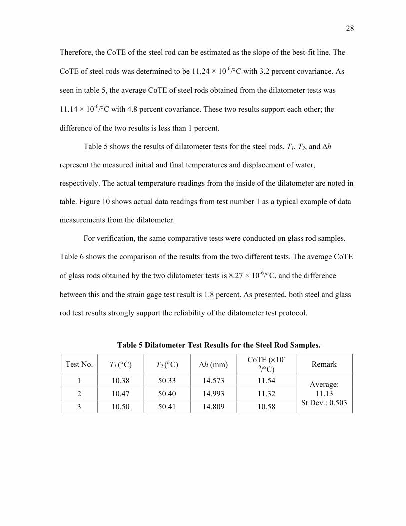
Therefore, the CoTE of the steel rod can be estimated as the slope of the best-fit line. The
CoTE of steel rods was determined to be 11.24 × 10⁻⁶/°C with 3.2 percent covariance. As
seen in table 5, the average CoTE of steel rods obtained from the dilatometer tests was
11.14 × 10⁻⁶/°C with 4.8 percent covariance. These two results support each other; the
difference of the two results is less than 1 percent.
Table 5 shows the results of dilatometer tests for the steel rods. T1, T2, and ∆h
represent the measured initial and final temperatures and displacement of water,
respectively. The actual temperature readings from the inside of the dilatometer are noted in
table. Figure 10 shows actual data readings from test number 1 as a typical example of data
measurements from the dilatometer.
For verification, the same comparative tests were conducted on glass rod samples.
Table 6 shows the comparison of the results from the two different tests. The average CoTE
of glass rods obtained by the two dilatometer tests is 8.27 × 10⁻⁶/°C, and the difference
between this and the strain gage test result is 1.8 percent. As presented, both steel and glass
rod test results strongly support the reliability of the dilatometer test protocol.
Table 5 Dilatometer Test Results for the Steel Rod Samples.
Test No. T1 (°C) T2 (°C) ∆h (mm) CoTE (×10-
6/°C) Remark
1 10.38 50.33 14.573 11.54 2 10.47 50.40 14.993 11.32 3 10.50 50.41 14.809 10.58
Average: 11.13
St Dev.: 0.503

29
CoTE = 11.24×10⁻⁶/°C Std dev = 0.36 R2 =.983
-100
0
100
200
300
400
500
-20 -10 0 10 20 30Temperature (C)
Stra
in (x
10-6
)
steel set 1steel set 2Best Fit
Figure 9 Thermal Expansions of Steel Rod Samples Measured by Strain Gage.
Based on these results, a correction of 0.2 percent to the change in float level should
adequately calibrate and adjust the calculated CoTE, to the true value. This is an increase in
CoTE since the calibration results were lower than the true results.
Repeatability of Dilatometer Tests in Measuring Aggregate CoTE
Repeatability of the dilatometer test protocol was investigated by repeating the test on a
single aggregate sample. In fact, the verification tests described in the above section also
indicated good repeatability. Each of the three tests on the steel samples as well as the latter
two tests on the glass rods produced very similar CoTE values for each material set. In this
section, the Abilene limestone sample was tested three times and the results were
compared. Table 7 shows the comparisons of repeated test results.

30
(a) Temperature measurements
(b) Corresponding displacement of the water level at the tower of dilatometer
Figure 10 Typical Data Measurements of Dilatometer Tests.

31
Table 6 Comparison of CoTE of Glass Rods Obtained by Dilatometer and Strain Gage.
Test T1 (°C) T2 (°C) CoTE (×10-6/°C)
Dilatometer 1st 10.35 50.45 8.46
Dilatometer 2nd 10.28 50.31 8.08
Strain Gage -13.6 21.3 8.42
Table 7 Comparison of Repeated CoTE Tests for Abilene Limestone.
Test
Initial
sample
weight (g)
Volume
ratio
(Va/V)
T1 (°C) T2 (°C) ∆h (mm) CoTE
(×10-6/°C)
1 3967.2 0.4937 10.45 50.42 16.701 5.78
2 4054.4 0.5044 10.55 50.71 16.601 6.41
3 4054.4 0.5055 10.41 50.58 16.381 5.98
The initial sample weight is in SSD, condition and the volume ratio represents the
ratio of initial volume of aggregate sample (Va) to the initial total volume (V). The
dilatometer was not opened between tests 2 and 3 and was left in the water bath until it
cooled to room temperature so that the same sample was used for the last two tests. Note
that the initial volumetric relations are different even for those two tests because the
measured initial temperatures are different. Comparison of repeated test results indicated
that the dilatometer produces acceptable repeatability. The average CoTE of the three tests
is 6.05 × 10⁻⁶/°C with 5 percent.

32
Tests at Constant Temperature Conditions
Possible systematic errors of the test system were investigated by testing under two
different constant temperature conditions. In the first test, the dilatometer filled with water
and aggregate sample was placed in the water bath, which was maintained at a temperature
of 35°C. The data were collected as a normal CoTE test but longer period of time. The test
result indicated that at least 2 hours of resting time was required after the final temperature
was reached to get stable LVDT data. However, the maximum rebound of LVDT data is
about 0.05 mm, from which the resulted error in CoTE is less than 2 percent. For a normal
CoTE test, the displacement is averaged for at least 30 minutes data between 1.5 and 4
hours after the final temperature is reached. According to the trend of the LVDT data, the
current data reduction method seems to be reasonable.
In the second test, the dilatometer was placed in the water bath at room temperature
without operating the water bath and data were collected for 11 hours. The slight decrease
in measured temperature is believed to be caused by the decrease of the room temperature
during the night. The trend of the data shows (Figure 11) the conformity between test
volume and temperature.

33
(a) Temperature measurements
(b) Corresponding LVDT measurements
Figure 11 Data Collections at a Constant Temperature (35°C).
34
TESTING PROTOCOL
There are four steps in the volumetric dilatometer test:
1. preparing the sample,
2. vacuuming,
3. testing, and
4. analyzing the results. Preparing the Sample
A representative aggregate sample, one and one-half times the required volume, is selected.
The sample is properly washed to remove dust and unwanted particles, and is then
submerged in water to for at least 24 hours before starting of the test. After the sample is
taken out of water it is washed once again before placing it inside the dilatometer. The SSD
and the submerged weight of aggregate are taken using the Rice specific gravity method.
The volume of aggregate, Va, is calculated using the equation below:
)( SUBSSDa WWvV −⋅= (7)
where v = specific volume of water at the initial temperature,
WSSD = weight of aggregate sample in saturated surface dry condition,
WSUB = weight of aggregate sample submerged under water.
In equation (7), the temperature dependence of the aggregate volume is accounted by the
specific volume of water at the specific temperature. The weights are independent of
temperature.
The whole dilatometer is then filled with aggregate sample. The lid of the
dilatometer is screwed tightly and it is then filled with water to a certain level marked on
the lid window.

35
Vacuuming
Vacuuming is performed based on the guidelines provided in Appendix D.
Testing
The water level is set to the fixed position after vacuuming. The dilatometer is then placed
into the 24°C water bath. The LVDT is placed on the float rod through the tower. The float
is placed properly on the water surface by rotating the LVDT and observing the change in
reading on the monitor. The reading of the LVDT is monitored for 15 minutes more to
make sure that there is no leak from the dilatometer. Then the water bath temperature is
adjusted to the initial temperature (T1), i.e., 10°C. It takes around 0.5 hour to reach 10°C.
The temperature stabilizes at 10°C after 1.5 hours. The initial water temperature inside
dilatometer container and the position of the water surface (h1) are automatically recorded
by the data acquisition system. Then the temperature is changed to final temperature (T2),
i.e., 50°C. The position of the water surface at temperature T2, denoted by h2, is recorded by
the LVDT and the data acquisition system. Consequently, the rise of the water surface when
temperature is increased by )T from T1 to T2 is )h = h2 - h1.
Analysis
The average coefficient of thermal expansion of the aggregate from T1 to T2 can be
calculated from Va, V, ∆h, ∆T, γw, and γf with equations (4) and (5), where γf = 55..33 × 10-
5/°C. The dilatometer-measured CoTE values of the different types of aggregates are
presented in a later section.

36
4. MODELING APPROACH
INTRODUCTION
As already discussed in section 1 CoTE of the aggregate is mainly dependent on CoTE of
the constituent minerals and their respective volume in aggregate. In this context, a new
mineralogical approach to model aggregate CoTE has been introduced. Modeling of
coefficient of thermal expansion will provide the person to predict the CoTE values based
on the aggregate mineralogical contents and the mortar fraction in concrete. One can come
up with different designs based on different ratios of constituents for concrete and steel if
the specified CoTE value is met, without even doing much testing. This method reduces not
only the effort and expenses on sample preparation of concrete and testing but the time also.
Since aggregates are composite material consisting of different minerals in different
proportions, it is assumed that their properties can be determined from the properties of
component minerals (10). A composite model to predict aggregate CoTE by using the
CoTE of constituent minerals and their respective volume percentages has been introduced.
Accuracy of the aggregate CoTE prediction by this composite modeling is mainly
dependent on the accuracy of the CoTE of the individual pure minerals contained in the
aggregates. Volumetric dilatometer testing method (11), which has been established earlier
to measure aggregate and concrete CoTE (21), is used to accurately measure the CoTE of
individual pure minerals. CoTE of individual aggregate is also estimated by dilatometry.
Favorable comparison between the modeled and the measured aggregate CoTE provided a
logical approach to establish a mineralogical composite model as a means to predict the
aggregate CoTE. After determining the CoTE of aggregate, it is then attempted to predict
the concrete CoTE based on the same principal of composite modeling in two component

37
system i.e. aggregate and mortar. Like aggregate CoTE, predicted concrete CoTE is also
validated by drawing favorable comparison between predicted and measured concrete
CoTE.
Basically, there are two models that predict the properties of a composite from those
of its components: the parallel model and the series model. Constituent minerals in the
aggregate are the components in the aggregate CoTE model, whereas mortar and coarse
aggregate are the components in the concrete CoTE model. In the parallel model, the
components of a composite are assumed to be combined in parallel. In the case of concrete,
cement mortar and aggregate are the parallel components, as shown in Figure 12(a). When
the concrete is loaded, mortar and aggregate are both displaced, so that the strain in both the
components is same. The series model is illustrated in Figure 12(b), where the total
displacement of the concrete under a tension force is the sum of the displacement of the
constituent mortar and aggregate. The stress in the constituent mortar and aggregate is
uniformly distributed. Hirsch’s model (10) is a combination of the above two models and
which has been used to predict the elastic modulus of concrete (Figure 12(c)). The present
aggregate and concrete CoTE model is based on the concept of Hirsch’s composite model.
The derived formulae for the aggregate and concrete CoTE models based on
Hirsch’s composite model are presented later.
MODELING OF AGGREGATE CoTE
A model is proposed to predict aggregate CoTE based on the calculated mineral weight
percentages, measured pure mineral CoTE, and their modulus of elasticity (MOE). Minerals
present and their respective weight percentages in the aggregates are calculated from the
bulk chemistry (i.e., elemental oxide weight percentages of the aggregates). The CoTE of

38
common pure minerals was measured by dilatometry, and MOE of minerals were collected
from literature. The prediction model for the aggregate CoTE is then formulated based on
Hirsch’s composite model (10).
Materials and Test Methods
Five different types of commonly used aggregates, namely, siliceous river gravel (SRG),
calcareous river gravel (CRG, mainly calcareous with siliceous impurities), pure limestone,
sandstone, and granite were collected from different areas across the state of Texas. CoTE
was determined on samples of five pure minerals, namely, calcite, quartz, dolomite, albite
(Na-feldspar), and microcline (K-feldspar) obtained from Ward’s Natural Science Est. Inc.
by dilatometry tests. These five minerals represent, to a large extent, the expected
mineralogy of the above aggregates. The effect of other commonly occurring minor
minerals (e.g., pyroxenes, magnetite/hematite, micas) on aggregate (e.g., granite) CoTE was
assumed to be insignificant.

39
Figure 12 Composite Models for Concrete CoTE Calculation: (a) Parallel Model (b) Series Model (c) Hirsch’s Model.
40
Bulk chemical analyses of representative powder samples of the above aggregates
were carried out by X-ray fluorescence (XRF) at Wyoming Analytical Laboratories, Inc.,
located in Golden, Texas. Calculated mineralogy obtained by the proposed model
(discussed later) for each aggregate was verified by X-ray diffraction (XRD, Rigaku
Miniflex) at Texas Transportation Institute (TTI). Concrete cylinders of 8 × 4 inches were
cast using the above-mentioned coarse aggregates, fine aggregate (single source), type I
cement, and fly ash with 0.42 water/(cement + fly ash) ratio. A standard mortar using the
same sand and maintaining the same ratio of sand:cementitious materials in concrete was
cast. Dilatometry (11) was used to measure the CoTEs of the individual pure minerals,
above-mentioned aggregates, mortar, and concrete. Cylindrical mortar and concrete
specimens (5.6 × 4 inch) were obtained from the original 8 × 4 inch specimens, and
measurement of CoTE by dilatometer was performed after 28 days of moist curing.
Representative samples from as-received loose aggregate were prepared following the
protocol explained in Appendix E and used to measure aggregate CoTE.
Elemental oxide weight percentages for all prepared aggregate powder samples
were determined by XRF and are presented in Table 8.
Determination of Mineral Weight Percentages from Bulk Chemical Analysis
As previously noted, minerals present in an aggregate source and their respective weight
percentages can be estimated from the elemental oxides as determined by chemical
analyses. Two different schemes of calculation were proposed to determine mineral weight
percentages from bulk chemical analysis of aggregate. This calculation represents a wide
range of rocks (i.e., sedimentary, igneous, and their metamorphic equivalents) commonly

41
used as aggregates and provides a realistic representation of the mineral phases present in
different types of aggregate.
Table 8 Bulk Chemical Analyses of the Tested Aggregates.
Bulk chemical analyses (wt%) Aggregate Sample No. SiO2 Al2O3 Fe2O3 CaO MgO Na2O K2O LOI 1 94.17 0.93 0.94 1.78 0.00 0.22 0.28 1.68 Gravel
(siliceous) SRG
2 96.86 0.79 1.01 0.54 0.11 0.00 0.14 0.55
3 35.57 1.20 2.30 32.20 1.50 0.00 0.30 26.46 Gravel* (calcareous), CRG
4 22.13 0.29 2.72 40.31 1.39 0.00 0.24 32.67
5 2.28 0.47 0.24 53.76 0.52 0.00 0.05 42.53 6 0.26 0.11 0.04 55.33 0.39 0.01 0.01 43.73 7 2.57 0.24 0.65 53.07 0.61 0.00 0.07 42.39 8 5.97 0.23 0.86 51.07 0.86 0.00 0.07 40.92 9 6.21 0.11 0.06 51.53 0.86 0.05 0.01 41.17 10 0.34 0.00 0.08 54.16 1.67 0.08 0.02 43.65
Limestone (Lst)
11 0.24 0.00 0.03 56.16 0.15 0.00 0.00 43.42 12 79.84 8.43 4.51 1.09 0.845 1.43 1.95 1.67 Sandstone
(Sst) 13 90.16 2.70 3.28 0.62 0.22 0.30 0.58 2.13 14 72.14 13.62 3.28 1.24 0.28 3.86 4.92 0.02 Granite
15 68.97 13.45 5.21 2.18 0.80 3.72 4.23 0.21 *Mainly calcareous with siliceous impurity.
Method I
This method was used to calculate weight percentages of seven minerals (dolomite,
albite, orthoclase, anorthite, quartz, calcite, and magnetite) and is applicable to aggregates
belonging to the sedimentary group of rocks and their metamorphic equivalents (e.g.,
limestone, gravel, sandstone, marble, etc). These seven minerals cover the major
constituents in most sedimentary rocks and their metamorphic equivalents, which are
commonly used as aggregates. This calculation method is based on an allotment of
elemental oxide weight percentages to mineral weight percentages according to
stoichiometric chemical equations for minerals (Appendix F). This method is not used for
shale, siltstone, or schist rocks because of limitations in calculating the micaceous and clay

42
minerals. However, the practice of using these types of rocks as concrete aggregate is
somewhat limited. The following assumptions were considered for simplification of the
calculation (Appendix F):
• All SiO2 is allocated to quartz and feldspar. The three most commonly occurring
types of feldspar (i.e., potassium feldspar [orthoclase/microcline], sodic-feldspar
[albite] and calcium feldspar [anorthite] are considered for the calculation.
• All CaO is allocated to calcite, dolomite (to combine all MgO), and anorthite (to
combine, if any, leftover Al2O3 after orthoclase and albite).
• All Fe2O3 is allocated to magnetite or hematite because chemical analysis generally
includes all Fe in Fe2O3 or FeO.
Method II
This method is used to calculate weight percentages of nine minerals (apatite,
ilmenite, orthoclase, albite, anorthite, pyroxenes, olivine, quartz, and magnetite/hematite)
and is applicable to aggregates belonging to the igneous suite of rocks and their
metamorphic equivalents (e.g., granite, basalt, granulites, and ultrabasic rocks, etc).
Method I cannot be used to calculate the mineralogy of these rocks because:
1. The allotment of SiO2 only to feldspars and quartz (method I) is not valid for these
rock types. Ferromagnesian silicates (e.g., pyroxene, olivine) are essential mineral
phases in these suites of rocks and they also contain SiO2. Ultrabasic rocks do not
contain quartz, which can only be reflected by method II.
2. Calcite and dolomite are not present in the igneous suite of rocks as a primary
crystallizing phase. Therefore, allotment of CaO to calcite and dolomite is not valid

43
for these groups of rocks where the primary source of CaO is Ca feldspar (anorthite)
with minor contributions from pyroxenes (e.g. diopside) and amphiboles.
The calculation of method II is based on proper sequential allotment of the
molecular proportion of elements to mineral weight percentages based on the crystallization
sequence in magma. Detailed steps for the calculation of method II are presented in
Appendix F.
The following selection criteria were followed based on bulk chemical analysis to
determine the suitable method for the sampled aggregate:
• SiO2 ≥ 80 percent (e.g., sandstone, fine sand aggregates, siliceous gravel, metaquartzite, etc.) - Method I
• CaO ≥ 30 percent and LOI ≥ 25 percent (e.g., limestone, marble, etc.) - Method I • SiO2 = 38-75 percent, Al2O3 = 10-18 percent and CaO < 20 percent (igneous rocks,
e.g., granite, rhyolite, andesite, diorite, basalt, gabbro, etc.) - Method II
The proposed methods were applied to calculate mineral weight percentages from bulk
chemical analysis of the respective aggregate powder samples and are presented in Table 9.
Table 9 also shows the presence of actual minerals identified by XRD. A perusal of Table 9
shows that calculated mineralogy based on the proposed method closely resembles with the
actual mineralogy identified by XRD. This supports the capability of the proposed method
to calculate the mineralogy in a more realistic manner.

44
Table 9 Calculated Mineral Volume (Percent) by the Proposed Methods for the Tested Aggregates along with Actual Minerals Identified by XRD for Some
Selected Aggregates.
Mineral volume (%) Aggregate Samp.
No. Do Cc Ab An Pf Qtz Mt Pyx
Minerals
identified
from XRD
1 0.00 2.73 1.91 0.69 1.71 92.25
0.69 0.00 Qtz SRG METHOD I 2 0.47 0.06 0.00 1.69 0.85 96.1
8 0.75 0.00
3 6.71 51.92
0.00 2.44 1.90 35.23
1.79 0.00 CRG METHOD I 4 6.27 67.5
0 0.00 0.01 1.37 20.8
7 3.88 0.00 Cc, Qtz,
Ab (t), Do (t)
5 2.37 94.23
0.00 1.17 0.32 1.71 0.19 0.00
6 1.77 97.73
0.09 0.24 0.06 0.07 0.03 0.00 Cc, Ab (t), Do (t)
7 2.80 93.29
0.00 0.45 0.41 2.11 0.94 0.00
8 3.92 88.58
0.00 0.44 0.45 5.92 0.68 0.00
9 3.90 89.22
0.46 0.05 0.06 6.26 0.05 0.00
10 7.57 91.96
0.73 0.00 0.13 0.00 0.06 0.00 Cc, Ab (t), Do (t)
Limestone METHOD I
11 0.68 99.04
0.00 0.00 0.00 0.26 0.02 0.00
12 3.56 0.00 12.13
10.46
11.60
58.95
3.31 0.00 Sandstone METHOD I 13 0.96 0.00 2.66 4.29 3.61 86.9
3 2.51 0.00
14 0.00 0.00 32.66
5.31 29.08
24.85
0.00 6.29 Qtz, Ab, Pf, Pyx, Biotite,
Muscovite
Granite, METHOD II
15 0.00 0.00 31.48
7.50 25.00
22.33
0.00 11.31
D – Dolomite, Cc – Calcite, Ab – Albite (Na-feldspar), Pf – K-feldspar, Qtz – Quartz, Mt – Magnetite, Pyx – Pyroxene; t – trace amount

45
CoTE of Pure Minerals
The CoTEs of five natural pure minerals (calcite, dolomite, albite, orthoclase, and quartz)
were measured by dilatometer and are presented in Table 10. These five pure minerals
constitute the majority of expected mineralogy of the tested aggregates. The cylindrical 5.6
× 4 inch specimens were obtained from the bigger sized mineral specimens by coring and
were used to measure CoTE in the dilatometer. Calcite, dolomite, and quartz were
polycrystalline type, whereas albite and orthoclase were selected from cleaved blocks.
Powder samples of the all the collected minerals were prepared and analyzed by XRD to
check their purity. The minor phases identified as impurities are also listed in Table 11.
Note that the minerals in natural aggregates also contain similar types of impurities.
Therefore, the measured CoTE of these naturally occurring minerals with traces of
impurities provides a more realistic mineral CoTE input for the aggregate CoTE modeling.
Composite Modeling to Predict Aggregate CoTE
The model to predict aggregate CoTE is based on the concept of Hirsch’s composite model
(10), where determined CoTE of pure minerals and their respective volume percent are the
two main inputs. The following formula is derived based on Hirsch’s composite modeling
to predict aggregate CoTE:
( )1 i i ia i i
i i
V Ex V x
V Eα
α α = + −
∑∑ ∑ (8)
where αa = CoTE of aggregate,
αi = CoTE of individual mineral,
Vi = volume fraction of each mineral in aggregate, and
Ei = Young’s modulus of each mineral phase.
46
X= relative proportions of material conforming with the upper and lower bound
solution.
Hirsch’s model becomes the series model when X = 0, and it becomes the parallel
model when X = 1. A value of 0.5 is assumed for X and indicates that the chance of
occurrence of either parallel or series arrangements of the constituent minerals in the
aggregate is equal. The predicted aggregate CoTE based on CoTE and elastic modulus of
pure minerals (Table 11) (22) and their respective calculated mineral volume percent are
presented in Table 12. The CoTEs of all the sampled aggregates were measured by
dilatometer and are also listed in the same table for comparison. Figure 13 shows the
graphical representation of measured vs. calculated CoTE of aggregates.
Table 10 Comparative Assessments between Mineral CoTE (Linear) Measured by
Dilatometer and Collected from Literature.
Mineral Dilatometer ASTM STP 169C Handbook (22) Dolomite 9.62 - 9.40* Calcite 5.58 5.0 5.05* Albite 6.52 6.0 6.00* Anorthite - 3.0 4.70+ Microcline 6.50 6.5-7.5 5.20+ Quartz 13.00 12.0 - Magnetite - - 6.86+ Pyroxene - 6.5 – 7.5 12.11*
*Average of 3 linear CoTE along three crystallographic direction (a,b,c) of single crystal; + linear CoTE = volume CoTE / 3

47
Table 11 CoTE of the Pure Minerals Measured by Dilatometer, Their Respective Elastic Modulus and Phases Identified as Impurities by XRD.
Minerals CoTE
measured (10-6 /oC)
CoTE from literature (22) (10-6/oC)
Elastic modulus (× 106 psi) (22)
Traces of minerals identified as impurity by XRD
Calcite 5.58 20.42 No impurity Dolomite 9.62 29.07 1.Ankerite
[Ca(Fe,Mg)(CO3)] 2.Minrecordite [CaZn(CO3)]
Quartz 13.00 12.30 No impurity Microcline 6.60 9.50 Disordered albite
(NaAlSi3O8) Albite 6.80 10.50 Anorthite
(CaAl2Si2O8) Anorthite 4.70 17.60 Albite (NaAlSi3O8) Magnetite 6.86 38.30 Pyroxene 12.11 32.50
Table 12 Mineral Volumes (Percent) and Calculated CoTE for the Tested Aggregates
along with Measured CoTE by Dilatometer.
Mineral volume (%) CoTE (10-6/°C)
Aggregate Sample No.
Do Cc Ab An Pf Qtz Mt Pyx Cal. Msd. 1 0.00 2.73 1.91 0.69 1.71 92.25 0.69 0.00 12.39 12.30 SRG
Method I 2 0.47 0.06 0.00 1.69 0.85 96.18 0.75 0.00 12.70 13.10 3 6.71 51.92 0.00 2.44 1.90 35.23 1.79 0.00 8.20 9.19 CRG
Method I 4 6.27 67.50 0.00 0.01 1.37 20.87 3.88 0.00 7.23 5 2.37 94.23 0.00 1.17 0.32 1.71 0.19 0.00 5.81 6.35 6 1.77 97.73 0.09 0.24 0.06 0.07 0.03 0.00 5.67 6.74 7 2.80 93.29 0.00 0.45 0.41 2.11 0.94 0.00 5.87 6.27 8 3.92 88.58 0.00 0.44 0.45 5.92 0.68 0.00 6.14 9 3.90 89.22 0.46 0.05 0.06 6.26 0.05 0.00 6.15 6.45 10 7.57 91.96 0.73 0.00 0.13 0.00 0.06 0.00 5.96
Limeston e Method I
11 0.68 99.04 0.00 0.00 0.00 0.26 0.02 0.00 5.63 12 3.56 0.00 12.13 10.46 11.60 58.95 3.31 0.00 10.35 10.30 Sandstone
Method I 13 0.96 0.00 2.66 04.29 3.61 86.93 2.51 0.00 12.05 12.00 14 0.00 0.00 32.66 5.31 29.08 24.85 0.00 6.29 8.93 8.81 Granite,
Method II
15 0.00 0.00 31.48 7.50 25.00 22.33 0.00 11.31 9.28 9.00
Cal. – Calculated, Msd. – measured; Do – Dolomite, Cc – Calcite, Ab – Albite (Na-feldspar), Pf – K-feldspar, Qtz – Quartz, Mt – Magnetite, Pyz – Pyroxene

48
Perusal of Figure 13 shows that the predicted CoTE by modeling closely resembles
the measured CoTE as is evident from higher correlation coefficients (0.98) between
calculated and measured CoTE. Calcareous gravel (impure limestone) deviates slightly
from the main trend. Calcareous gravels show slightly higher measured CoTE (9.19 × 10-
6/°C) than the predicted CoTE (8.2 × 10⁻⁶/°C). However, additional testing of other
calcareous gravels needs to be performed in order to verify whether this type of aggregate
always shows slightly higher measured than predicted CoTE.
Aggregate source variability should be reflected in variations in elemental oxide
weight percentages if properly sampled. Variation in elemental oxide weight percentages
results in mineralogy changes and, hence changes in CoTE. As, for example, the CoTE of
pure limestone is 5.7- 6.2 × 10⁻⁶/°C, whereas, that of impure siliceous limestone is give 7.2-
8.2 × 10⁻⁶/°C. Therefore, the present mineralogical modeling approach is a sensitive tool to
monitor the aggregate source variability and has great potential for aggregate quality
control.

49
Figure 13 Calculated vs Measured Aggregate CoTE.
MODELING OF CONCRETE COTE
The model to predict concrete CoTE is based on the concept of Hirsch’s composite model,
where determined CoTEs of mortar and coarse aggregate are the two main inputs. Our
proposed concrete CoTE model is basically a two-step model (i.e., (i) prediction and
validation of aggregate CoTE, elaborated in the foregoing discussion, and (ii) prediction of
concrete CoTE based on calculated CoTE of aggregate in the first step (Table 12) and
known CoTE of standard mortar). Measured concrete CoTE by dilatometer validates the
concrete CoTE model by comparing the predicted value to the measured value. The
following formula is derived based on Hirsch’s composite modeling to predict concrete
CoTE:
aamm
aaammmaammc EVEV
EVEVXVVX
++
−++=αα
ααα )1()( (9)
where αm, αa = CoTE of mortar and aggregate,

50
Vm, Va = volume fraction of mortar and aggregate,
Em, Ea = elastic modulus of mortar and aggregate, and
X = relative proportions of material conforming with the upper and lower
bound solution.
The CoTE of a standard mortar specimen (14.5 × 10⁻⁶/°C) using the same sand and
similar sand: cement ratio that was used in the concrete was measured by dilatometer and
used as the fixed-mortar CoTE input in the concrete CoTE model. Volume fractions of
mortar and aggregate are calculated from mixture proportions of the tested concrete
specimens and are given in Table 13. A value of 1× 10⁶ psi was used as the fixed input for
MOE of mortar. It is observed that MOEs of 5-10 × 106 psi represent nearly all natural
rocks commonly used as aggregates. Research have found from modeling of elastic
modulus that, at least for some concretes, X is approximately 0.5 (23). Therefore, 0.5 was
assigned for X in the present study.
Cast concrete specimens (cylindrical 8 × 4 specimens) were sliced into 4 (diameter)
× 5.5 (height) inch dimensions after 28 days of moist curing. The CoTE of these sliced
cylindrical specimens was measured by dilatometer after curing them in 100 percent
humidity chamber for 28 days. Predicted and measured concrete CoTEs are presented in
Figure 14. Perusal of figure indicates that predicted CoTE shows good correlation with
measured CoTE, with correlation coefficient of around 0.97. The effect of changing
aggregate MOE (from 5× 10⁶ to 10 × 106 psi) on predicted concrete CoTE was also
checked. It was observed that the predicted concrete CoTE slightly decreases with
increasing aggregate MOE. It is interesting to note that the correlation coefficient between
predicted and measured CoTE remains unchanged while changing aggregate MOE.
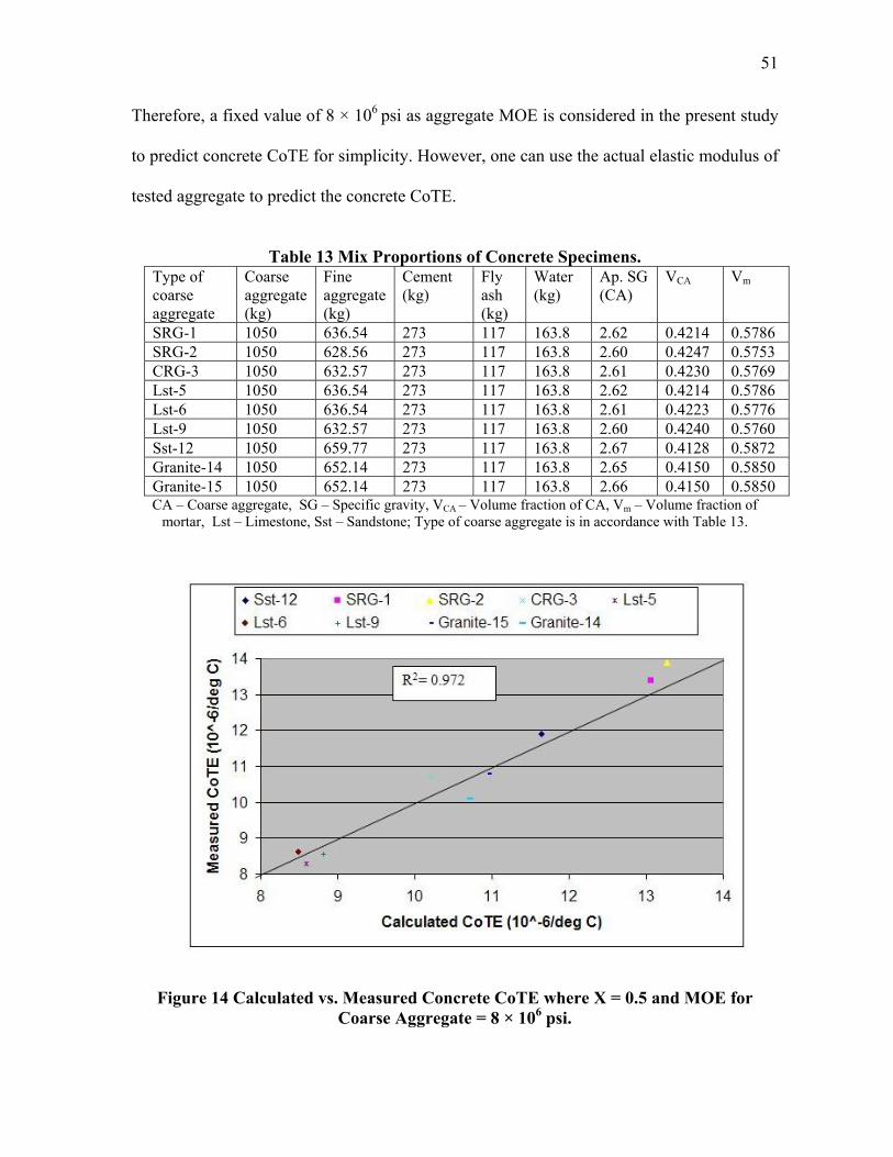
51
Therefore, a fixed value of 8 × 10⁶ psi as aggregate MOE is considered in the present study
to predict concrete CoTE for simplicity. However, one can use the actual elastic modulus of
tested aggregate to predict the concrete CoTE.
Table 13 Mix Proportions of Concrete Specimens.
Type of coarse aggregate
Coarse aggregate (kg)
Fine aggregate (kg)
Cement (kg)
Fly ash (kg)
Water (kg)
Ap. SG (CA)
VCA Vm
SRG-1 1050 636.54 273 117 163.8 2.62 0.4214 0.5786 SRG-2 1050 628.56 273 117 163.8 2.60 0.4247 0.5753 CRG-3 1050 632.57 273 117 163.8 2.61 0.4230 0.5769 Lst-5 1050 636.54 273 117 163.8 2.62 0.4214 0.5786 Lst-6 1050 636.54 273 117 163.8 2.61 0.4223 0.5776 Lst-9 1050 632.57 273 117 163.8 2.60 0.4240 0.5760 Sst-12 1050 659.77 273 117 163.8 2.67 0.4128 0.5872 Granite-14 1050 652.14 273 117 163.8 2.65 0.4150 0.5850 Granite-15 1050 652.14 273 117 163.8 2.66 0.4150 0.5850 CA – Coarse aggregate, SG – Specific gravity, VCA – Volume fraction of CA, Vm – Volume fraction of
mortar, Lst – Limestone, Sst – Sandstone; Type of coarse aggregate is in accordance with Table 13.
Figure 14 Calculated vs. Measured Concrete CoTE where X = 0.5 and MOE for Coarse Aggregate = 8 × 10⁶ psi.

52
5. SUMMARY AND CONCLUSION
This report discussed the volumetric dilatometer test method to measure aggregate
and concrete CoTE. The new approach to predicting the aggregate and concrete CoTE
based on the mineralogy of the aggregate and the mix proportions of the concrete is also
well elaborated.
Under a change in temperature, an unrestrained material will change shape
proportional to the amount of temperature change multiplied by its coefficient of thermal
expansion. The CoTE indicates how much material shape will change for each degree of
temperature change. The CoTE is, therefore, a fundamental engineering property that
quantifies the change in unit length per degree of temperature change. This will be a factor
to determine the type of aggregate can be used to keep the crack of a concrete pavement to
a maximum specified width because crack width is one factor which determines the load
transfer efficiency of concrete pavements.
As aggregates themselves comprise of a variety of minerals, it has been shown that
their CoTE varies with mineralogical composition and porosity. Quartz has the highest
CoTE of any common mineral, and aggregates with high quartz content have high CoTE
values. The CoTE of hardened concrete is variable, depending on the mixture design and
the type of aggregate used. Since aggregates make up the bulk of concrete, their properties
will largely determine concrete’s CoTE. With a known mixture proportion, the CoTE of
hardened concrete can be estimated from a weighted average of all its components.
53
CONCLUSION
A new mineralogical approach is presented to predict aggregate and concrete coefficient of
thermal expansion based on Hirsch’s composite modeling. The following points are drawn
as conclusions from the present study:
• The sampling protocol for the aggregate provides a consistent means to select a
representative powder sample for bulk chemical analysis. However, more care
should be taken for sampling gravel (especially calcareous gravel) aggregate.
• All three types of rocks (e.g., sedimentary, igneous, and metamorphic) commonly
used as aggregates can be considered in the present model by maintaining their
separate entity.
• Different aggregates are well represented by the weight percentage of minerals
actually present. The calculated mineralogy based on the proposed modeling and
actual mineralogy from XRD compare well. This similarity suggests that the
combination of the proposed two methods is capable of calculating representative
mineralogy for all types of aggregates.
• Dilatometer CoTE measurement of five pure minerals is fundamental to the
development of a model for the prediction of aggregate CoTE. More accurate
estimation of a pure mineral’s CoTE leads to more accurate the better will be the
prediction because individual mineral CoTE is the most important input when
calculating aggregate CoTE.
• Predicted aggregate CoTE by mineralogical modeling compares well with the
measured aggregate CoTE, except for with some minor deviation in calcareous
gravel. This similarity validates the composite model for prediction of aggregate
54
CoTE. However, more research on different types of aggregates is needed to
establish this resemblance, and hence, the effectiveness of composite mineralogical
modeling to predict aggregate CoTE.
• Different aggregates contain different types of minerals, and this is well reflected in
the proposed model. This difference in mineralogy gives rise to different CoTEs.
Therefore, present mineralogical modeling is sensitive to categorizing aggregates
based on their CoTE values.
• Predicted concrete CoTE by composite modeling and measured concrete CoTE by
dilatometer shows good correlation. This correlation validates the effectiveness of
composite modeling to predict concrete CoTE. A change of aggregate MOE from 5
× 106 psi to 10 × 106 psi does not result in significant variation in concrete CoTE.
Therefore, the composite model for prediction of concrete CoTE can be applied to
concrete containing a wide variety of aggregates with different CoTEs and MOEs.
Composite modeling will be useful as a check of aggregate source variability in
terms of quality control measures and improved design and quality control measures of
concrete. Further research needs to be done to test porous aggregates using dilatometer
device.
The overall strategy to implement the measurement and specification of CoTE is
shown in Figure 15 are divided into two main sections

55
Figure 15 Schematic of Overall CoTE Implementation Strategy.
QUALITY CONTROL (QC) TESTING ON THE AGGREGATE SOURCE
In concept, coarse aggregates taken from various sources can be sampled at specified
intervals. After chemical analysis of the mineral composition of the aggregates, the
coefficient of thermal expansion of coarse aggregates (αCA) can be predicted from results of
chemical or dilatometer testing. The aggregate coefficient of expansion (αCA) is used along
with the concrete mixture proportions to calculate the CoTE of the concrete. As shown in
Figure 15, the CoTE of the concrete mixture (αConc) is then estimated based on a weighted
average of all the mixture components, which include the coarse aggregate (CA), fine
aggregate (FA), and the hydrated cement paste (HCP).
QUALITY ASSURANCE (QA) TESTING ON THE CONCRETE
During construction, QA testing on the concrete will be performed at specified intervals.
The specimens for this test will involve either the concrete as delivered to site (cylinders or
beams) or the concrete as placed (cores). Long-term pavement performance is related to the
56
in-situ CoTE value achieved, and enforcement could, therefore, eventually be based the
percentage of design life that will result due to the CoTE as constructed.
SPECIFICATION DEVELOPMENT
Development of a draft specification (Appendix G) will provide guidelines for CoTE that
ensure that design conditions are achieved during construction. The variability of
aggregates and concrete CoTE values need to be addressed as part of the specification as
well as aggregate prequalification, quality control testing, and quality assurance testing
during actual construction.
The CoTE implementation approach for the QC and QA testing phases were
previously shown in Figure 15. Quality control testing on the raw aggregate sources would
eliminate the need for concrete samples. Quality control testing can either be based on
chemical testing of the aggregate mineralogy or on dilatometer results. The required
sampling procedure and frequency of testing are explained in Section 4.
Quality assurance testing should be performed on the hardened concrete. This is
necessary to validate that the CoTE of the concrete as constructed meets the CoTE assumed
during design. The dilatometer is recommended to determine the CoTE of concrete
specimens. Ideally, the CoTE from samples cored out of the pavement should be tested, but
it can also be determine, from molded specimens collected onsite. Six inch cylinders can be
used for this purpose, but this would require that additional CoTE specimens be made. The
other possibility is that 6 inch beams, commonly used for strength testing, be used for
quality assurance testing. The frequency of quality assurance testing will also be addressed
in the specifications.

57
CLASSIFICATION OF AGGREGATES BASED ON TEXTURE AND CoTE
The classification of the coarse aggregate can be done in a format of Tα-N where
• T represents the measure of aggregate texture that ranges from 0 to 1200, e.g., L –
Low texture (<400), M – Medium texture (400-800), H – High texture (>800)
• α represents the measured CoTE of the aggregate in whole number of micro strain
/°C with a range of 5 to 12 (2.78 to 6.66 micro strain /°F), e.g., L – low, M- Medium
and H- High (refer Table 2).
• N represents name of the aggregate, e.g., siliceous river gravel (SRG), calcareous
river gravel (CRG), limestone (LST), sandstone (SST), Granite (GRN)
A perusal of Table 14 below illustrates the aggregate classification system in the above
Tα -N format
Table 14 Aggregate Classification System in Tα -N Format
Texture (T) CoTE ( α ) Aggregate name (N) Classification in
T α -N format Low texture (L) High (H) SRG-uncrushed LH-SRGUC Low texture (L) High (H) SRG-crushed (e.g. chert
dominated gravel) LH-SRGC
Medium texture (M) High (H) SRG-crushed (quartzite dominated gravel)
MH-SRGC
Medium texture (M) Low (L) Limestone - LST ML-LST Low texture (L) Low (L) Limestone - LST LL-LST Medium texture (M) Medium (M) Siliceous limestone -
SLST MM-SLST
Medium texture (M) Low (L) Marble (MRB) ML-MRB Low texture (L) Medium (M) CRG-uncrushed LM-CRGUC Medium texture (M) Medium (M) CRG-crushed MM-CRGUC High texture (H) Medium (M) Granite - GRN HM-GRN Low texture (M) Medium (M) Basalt - BST LM-BST Medium texture (M) High (H) Sandstone - SST MH-SST
Aggregate CoTE is classified in three categories based on their affect on concrete
pavements. Low CoTE value of aggregate is desired for better performance of pavements.

58
REFERENCES
1. McCullough, B. F., D. G. Zollinger, and T. Dossey. Evaluation of the Performance of Pavements Made with Different Coarse Aggregates. Research Report 3925-1F. Center for Transportation Research, The University of Texas at Austin, September 1998.
2. Mitchell, L. J. Thermal Expansion Tests on Aggregates, Neat Cements, and Concrete.
ACI Journal, Vol. 48, June 1953, pp. 964-977. 3. Meyers, S. L. How Temperature and Moisture Changes May Affect Durability of
Concrete. Rock Products, Vol. 54, No. 8, August, 1951, pp. 153-162. 4. Huang, Y. H. Pavement Analysis and Design. Prentice Hall, Englewood, New Jersey,
1993. 5. Neville, A. M. Properties of Concrete. John Wiley and Sons, New York, New, 1997. 6. Brown, R. D. Thermal Movement of Concrete. Current Practice Sheet, No. 3PC/06/01,
Cement and Concrete Association, Wexham Springs, Slough, England, November 1972.
7. Won, M., K. Hankins, and B. F. McCullough. Mechanistic Analysis of Continuously
Reinforced Concrete Pavements Considering Material Characteristics, Variability, and Fatigue. Report No. 1169-2, Center for Transportation Research, The University of Texas at Austin, April 1990.
8. Davis, R. E. A Summary of the Results of Investigations Having to Do with Volumetric
Changes in Cements, Mortars and Concrete, due to Causes Other Than Stress. ACI Journal, Proceedings 26, June 1930, pp. 407- 443.
9. Mullen, W. G., D. L. Bloem, and S. Walker. Effects of Temperature Changes on
Concrete as Influenced by Aggregates. ACI Journal, Vol. 48, April 1952, pp. 661-679. 10. Hirsch, T. J. Modulus of Elasticity of Concrete Affected by Elastic Moduli of Cement
Paste Matrix and Aggregate. ACI Journal, Vol. 59, No. 3, March 1962, pp. 427-451. 11. Zollinger, D. G., T. Tianxi, D. Fowler, and L. Wang. Development of a Test Apparatus
to Measure Thermal Expansion of Concrete Aggregates. Unpublishd Research Report (2992-1), Texas Transportation Institute, Texas A&M University System, College Station, 1998.
12. Willis, T. F., and M. E. DeReus. Thermal Volume Change and Elasticity of Aggregates
and Their Effect on Concrete. Proceedings, American Society for Testing and Materials, Vol. 39 pp. 919- 928.
13. Corps of Engineers, U. S. Army. Handbook for Concrete and Cement. Complete
Edition, Waterways Experiment Station, Vicksburg, Mississippi, August 1949.

59
14. Venecanin, S. D. Thermal Incompatibility of Concrete Components and Thermal
Properties of Carbonate Rocks. ACI Materials Journal, Vol. 87, 1990, pp. 602-607. 15. Mitchell, L. J. Thermal Expansion Test on Aggregate, Neat Cement and Concrete.
Proceedings, American Society for Testing and Materials, Vol. 53, 1953 pp. 963-975. 16. Verbeck, G. J., and W. E. Hass. Dilatometer Method for Determination of Thermal
Efficient of Expansion of Fine and Coarse Aggregate. Highway Research Board, Proceedings of the Thirtieth Annual Meeting, Jan. 9-12, 1951 pp. 187- 192.
17. Thermal Coefficient of Portland Cement Concrete.
http://www.tfhrc.gov/pavement/pccp/thermal.htm, accessed 13 August 2004. 18. Dossy, T., B. F. McCullough, and A. Dumas. Effects of Aggregate Blends on the
Properties of Portland Cement Concrete Pavements. Research Report 1244-8, Center for Transportation Research, The University of Texas at Austin, August 1994.
19. Gnomix pvT High Pressure Dilatometer.
http://www.datapointlabs.com/ExpCapShowDetails.asp?InstId=10 accessed 4 September 2004.
20. Handbook of Chemistry and Physics. 71st Ed., CRC Press, Boca Raton, Florida, 1990-
1991. 21. Shon, C. S., S. Lim, A. K. Mukhopadhyay, D. G. Zollinger, and S. L. Sarkar. New
Aggregate Characterization Tests for Thermal and ASR Reactivity Properties. Proceedings, ICAR 10th Annual Symposium, April 2002.
22. Ahrens, T. J., Mineral Physics and Crystallography, A Handbook of Physics Constants.
AGU Reference Shelf 2,American Geophysical Union, Washington, D.C. 1995. 23. Mindess, S., and J. F. Young. Concrete. Prentice Hall, Inc., Englewood Cliffs, New
Jersey, 1999.
60
APPENDIX A
RELATIONSHIP BETWEEN THE COEFFICIENT OF LINEAR
THERMAL EXPANSION AND THE COEFFICIENT OF
VOLUMETRIC THERMAL EXPANSION
The coefficient of linear thermal expansion and the coefficient of volumetric thermal expansion are designated by α and γ, respectively. When the temperature increases by ∆T, the volume of a body expands from V1 to V2. Any length within the body expands from L1 to L2. The coefficients " and γ are defined as follows:
L 2 = L 1 × (1+ ")T)
V 2 = V 1 × (1+()T) The relationship between α and γ is:
( = 3" This relationship holds for a body of any regular and irregular shapes. The relationships for the cylinder, and for any irregular shape are verified as follows. CYLINDER The volume of a cylinder with radius of r and height of h is: hrV 2
1 π=
After thermal expansion, the radius becomes r (1+a∆T) and the height becomes h (1+aDT), therefore, the volume of the cylinder becomes:
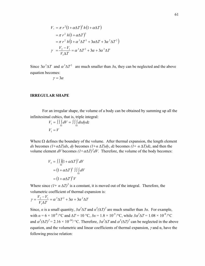
61
( ) ( )( )( )
TTTVVV
TTThrThr
ThTrV
∆++∆=∆−
=
∆+∆+∆+=
∆+=
∆+∆+=
223
1
12
22332
32
22
33
33 1 1
1 1 2
αααγ
αααπ
απ
ααπ
Since T∆23α and 23 T∆α are much smaller than 3α, they can be neglected and the above equation becomes: αγ 3=
IRREGULAR SHAPE For an irregular shape, the volume of a body can be obtained by summing up all the infinitesimal cubics, that is, triple integral:
VV
dxdydzdVV
=
∫∫∫=∫∫∫=ΩΩ
1
1
Where Ω defines the boundary of the volume. After thermal expansion, the length element dx becomes (1+α∆T)dx, dy becomes (1+α ∆T)dy, dz becomes (1+ α ∆T)dz, and then the volume element dV becomes (1+α∆T)3dV. Therefore, the volume of the body becomes:
( )
( )
( ) VT
dVT
dVTV
3
3
32
1
1
1
∆+=
∫∫∫∆+=
∆+∫∫∫=
Ω
Ω
α
α
α
Where since (1+ α ∆T)3 is a constant, it is moved out of the integral. Therefore, the volumetric coefficient of thermal expansion is:
TTTVVV
∆++∆=∆−
= 223
1
12 33 αααγ
Since, α is a small quantity, 3α2∆T and α3(∆T)2 are much smaller than 3α. For example, with α = 6 × 10⁻⁶ /°C and ∆T = 10 °C, 3α = 1.8 × 10⁻⁵ /°C, while 3α2∆T = 1.08 × 10⁻⁹ /°C and α3(∆T)2 = 2.16 × 10⁻¹⁴/ °C. Therefore, 3α2∆T and α3(∆T)2 can be neglected in the above equation, and the volumetric and linear coefficients of thermal expansion, γ and α, have the following precise relation:

62
αγ 3=
This relation is valid for a body of any shape.
63
APPENDIX B
CALIBRATION PROTOCOL FOR THE DILATOMETER
Following are the guidelines for calibration of dilatometer.
1. Run the device three times with distilled water to establish the gamma flask(γf) and its
coefficient of variation (COV)
• (COV = Xσ ; standard deviation divided by the mean) where the standard deviation
is based on a minimum of three consecutive tests.
• Recommended maximum. acceptable limit for the COV of the gamma flask is 1.5 percent
2. Run the device three times with a standard reference material (e.g., glass) to establish
the correction factor for ∆h and its COV based on a minimum of three consecutive tests:
• The correction factor for ∆h is the average of three ratios is determined from the
tests by dividing the ∆h of each test and the ∆h to exactly match the CoTE of the
reference material. Use the ‘∆h’ correction factor for all aggregate CoTE tests.
• Recommended maximum limit for the COV of the ∆h correction factor is 1.5
percent.
• By fixing the limits for steps 1 and 2, the variability from test to test will be limited
to an acceptable range. If the specified COV limits are not met, then repeat the test
until the measured COV falls below the required limit.
3. Run the device three times with any aggregate material (e.g., sandstone) to determine
aggregate CoTE and its actual CoTE COV:
• Calculated CoTE COV is based on the COV of the gamma flask and correction
factor for ∆h from spread sheet.

64
• Assign correction factor (if necessary) for calculated CoTE COV in order to match
the actual aggregate CoTE COV determined from the three tests (this value is
expected to be less than 5percent).
• Use this correction factor to adjust the calculated CoTE COV from the spreadsheet
for future tests.
Note: Repeat the calibration process every 30 tests or six months. Tests of highly porous
fine-grained sedimentary rocks (e.g., limestone, sandstone, etc.) must be checked for re-
saturation when the aggregate is held at 10ºC at the beginning of the test and at the end of
the test when the sample is held at 50ºC. The ∆h used to calculate the CoTE for these types
of aggregates must reflect the effects of re-saturation.

65
APPENDIX C
Variance Analysis
af
aw
f
a
f
twf V
V
V
V
TVhA γγγγ
10
10
10
10
10
+−∆
∆−=
( )
[ ]
[ ] ( )
( ) ( )( )
( )2
222
101010
10
)(
2))((
2))((
1
1
11010
10
hhCOVhVar
wwCOVwVar
ffCOVfVar
WWCovwG
WVarWVaVarV
XXVarX
X
XhVfVar
VVVTVV
VVhAV
a
iji
ui
i
ui
i
a
iwfaa
awf
aaa
ffwwaT
T
aa
∆∆=∆
=
=
=
∂∂
=
∂∂
∂∂
+
∂∂
=
=∆=
+=∆−=
−−+
∆∆
=
∑ ∑∑
γγγ
γγγ
γ
ργσγγ
γγγ
γ
γγγγ
( )
( ) ( )
( ) ( ) ( )
( ) ( )
)( 1
1
2
2
2.1
10102
10
22
22
2
2
fawa
wfaff
aawT
aa
wfaa
f
VarVVhVarT
AtV
VarVVVVarV
VVarhVarT
A
VVar
VarVVV
VaraVfV
aVarVaV
awaVarVhVar
TTA
aVaVar
γρ
γ
γγγ
γ
γγγ
++∆
∆+
−++
−+∆
∆=
−+
+
−+∆
∆=
Where V = total inner volume of the flask,

66
Vw = volume of water in the flask,
Vf = volume of the flask,
Va10 = volume of aggregate in the flask,
γa = coefficient of volumetric thermal expansion of aggregate,
γw = coefficient of volumetric thermal expansion of water, and
γf = coefficient of volumetric thermal expansion of flask,
A = inner sectional area of tower,
∆h = rise of the water surface inside the tower,
∆T = temperature increase from T1 to T2.

67
APPENDIX D
Guidelines for Vacuuming 1. Wash the aggregates thoroughly with distilled water to remove silts, clays, and other
fine materials. Select the required quantity of aggregate for the test and immerse in
distilled water.
2. Soak the washed aggregates overnight in a container to ensure a high degree of
saturation using distilled water.
3. After twenty four hours, transfer the aggregates to a Rice container (used to determine
the specific gravity of the material by the Rice method). Place a vacuum (29 inches of
mercury) on the container for 15 minutes to remove air trapped between the aggregate
particles.
4. Find the specific gravity of aggregates and volume of aggregates using rice method.
5. Transfer the aggregates from the Rice container to the dilatometer very carefully after
the dilatometer has been half-filled with distilled water to ensure that there is no air
trapped between the aggregate particles.
6. After ensuring against possible leakage, for less porous, coarse-grained, hard, and
compact aggregates (e.g., hard, compact, and fresh sandstone, granite, some gravel, and
marble) and concrete continue vacuuming for the next 60 minutes while checking that
the pressure gage needle does not fluctuate and that the mercury level in the cylinder is
near zero. Deviation from these conditions suggests possible leakage. An additional
period of vacuuming may be required in case of highly porous, fine-grained, weathered
sedimentary rocks (e.g., limestone, sandstone etc.). In case of standard reference
materials (e.g., glass, copper, steel, etc.) and water, experience has indicated 45 minutes
is sufficient to reduce the air bubble flow to a negligible level.

68
7. At the completion of each 15 minute vacuuming and vibration period, note the intensity
of the flow of air bubbles through the window in the tower before stopping. Intensity
may vary from sample to sample but it is recommended to continue the vacuuming until
the flow of air bubbles is reduced to a negligible level.
8. During the vacuuming process, it is helpful to apply vibration to the dilatometer. A
variable speed Gilson Vibro-Deairator (SGA-5R) was used at TTI. A specific
modification adapted the dilatometer to fit on the Vibro-Deairator. Maximum vibration
should be applied during the vacuuming process. The effectiveness of the vacuuming
de-airing can be monitored by observing the air bubble flow through the window in the
tower.

69
APPENDIX E
Sample Preparation A sampling protocol is introduced to obtain a representative powder sample; following are
the steps involved.
1. Thoroughly wash sample to remove foreign materials (i.e., soil, organics, etc.).
2. Visually inspect the samples with a magnifying glass to judge the aggregate
heterogeneity. Aggregate consisting of mainly one type of particles with respect to
shape, color, and texture are considered to be as homogeneous (e.g., crushed
limestone). On the other hand, aggregate with different types of particles with
respect to shape, color, grain size, and texture are considered to be heterogeneous
(e.g., gravel). Accurate judgment of heterogeneity is necessary for selecting
suitable methods in the following steps.
3. Cone and quarter the sample; the number of cycles of cone and quartering depend
on amount of sample needed and level of heterogeneity within the sample, as
suggested below (for one bag of sample, i.e., 50 lb):
• 1 cycle for highly heterogeneous samples, e.g., gravel.
• 2 cycles for intermediate samples, e.g., impure limestone, sandstones, etc.
• 3 cycles for homogeneous samples, e.g., pure limestone.
4. Dry the selected amount of sample overnight in oven at 60°C.
5. Crush the entire sample using a jaw crusher or similar type of device.
6. Cone and quarter the crushed sample. The Number of cycles is determined as
follows:

70
• 3 cycles for highly heterogeneous samples because the selected amount
before crushing is high.
• 1 or 2 cycles for homogeneous or less heterogeneous samples.
7. Grind the entire sample using a powdering device (e.g., pestle and mortar for small
quantities of sample or ball mill for larger quantities of sample particularly, in the
case of highly heterogeneous samples) to pass through a number 200 sieve (75 µm).
8. Analyze powder samples by XRF to determine the bulk chemistry.
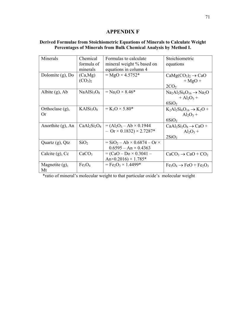
71
APPENDIX F
Derived Formulae from Stoichiometric Equations of Minerals to Calculate Weight Percentages of Minerals from Bulk Chemical Analysis by Method I.
Minerals Chemical
formula of minerals
Formulas to calculate mineral weight % based on equations in column 4
Stoichiometric equations
Dolomite (g), Do (Ca,Mg) (CO3)2
= MgO × 4.5752*
CaMg(CO3)2 → CaO + MgO + 2CO2
Albite (g), Ab NaAlSi3O8 = Na2O × 8.46* Na2Al2Si6O16 → Na2O + Al2O3 + 6SiO2
Orthoclase (g), Or
KAlSi3O8 = K2O × 5.80* K2Al2Si6O16 → K2O + Al2O3 + 6SiO2
Anorthite (g), An CaAl2Si2O8 = (Al2O3 – Ab × 0.1944 – Or × 0.1832) × 2.7287*
CaAl2Si2O8 → CaO + Al2O3 + 2SiO2
Quartz (g), Qtz SiO2 = SiO2 – Ab × 0.6874 – Or × 0.6595 – An × 0.4363
Calcite (g), Cc CaCO3 = (CaO – Do × 0.3041 – An×0.2016) × 1.785*
CaCO3 → CaO + CO2
Magnetite (g), Mt
Fe3O4 = Fe2O3 × 1.4499* Fe3O4 → FeO + Fe2O3
*ratio of mineral’s molecular weight to that particular oxide’s molecular weight

72
Sequential Allotment of Elemental Oxide Weight percent to Mineral Weight Percentages by Method II.
Calculation of molecular proportion (MP): divide the weight percentage (wt%) of each oxide by its molecular
weight to find the molecular proportion of that oxide
Minerals Chemical Formula Equations to calculate MP for minerals
Residual elemental oxide weight % after formation of a particular mineral
Apatite Ca5(PO4)(OH,F,Cl) = MP of P2O5 CaOI = CaOt – 3.33 × MP for apatite Ilmenite FeTiO3 = MP of TiO2
if FeO > TiO2 FeOI = MP of FeOt – MP of TiO2
Orthoclase (K-feldspar)
KAlSi3O8 = MP of K2O Al2O3 (I) = MP of Al2O3(t) – MP of K2O SiO2 (I) = MP of SiO2(t) – 6 × MP of K2O
Albite (Na-feldspar)
NaAlSi3O8 = MP of Na2O Al2O3 (II) = Al2O3(I) – MP of Na2O SiO2(II) = SiO2(I) – 6 × MP of Na2O
Anorthite (Ca-feldspar)
CaAl2Si2O8 = Al2O3(II) if CaOI > Al2O3(II)
CaOII = CaOI – Al2O3(II) SiO2(III) = SiO2(II) – 2 × Al2O3(II)
Anorthite
CaAl2Si2O8 = CaOI
if CaOI < Al2O3(II)
Al2O3(III) = Al2O3(II) – CaOI SiO2(III) = SiO2(II) – 2 × CaOI
Corundum Al2O3 = Al2O3(III) Magnetite Fe3O4 = FeOI
if Fe2O3(t) > FeOI Fe2O3(I) = Fe2O3(t) – FeOI
Magnetite Fe3O4 = MP of Fe3O4(t) if Fe2O3(t) < FeOI
FeO(II) = FeOI – Fe3O4(t)
Hematite Fe2O3 = Fe2O3(I) Diopside (Pyroxene)
(Ca,Mg)Si2O6 = CaOII
(MgO + FeO)R after diopside = (MgOt + FeOII ) - CaOII SiO2(IV) = SiO2(III) – 2× CaOII
Hypersthene (Pyroxene)
(Fe,Mg)SiO3 = (MgO+FeO)R if diopside is “YES”
SiO2(V) = SiO2(IV) – MP for hypersthene
Hypersthene (Fe,Mg)SiO3 = (MgOt + FeOII )
If diopside is “NO” SiO2(V) = SiO2(IV) – MP for hypersthene
Quartz SiO2 = SiO2(V) Multiplication of the above molecular proportions assigned to the respective phases by their molecular weight will give the weight % of respective minerals.
MP – Molecular proportion, t / (t) – total

73
APPENDIX G
Item 421 Special Provision
421.2. Materials.
E. aggregate.
1. Coarse aggregate. Coefficient of thermal expansion (CoTE) of coarse aggregate shall
not exceed the values specified by engineer when tested in accordance with Test Method
Tex-xxx. The Test method Tex-xxx is based on two approaches i.e., direct measurement by
Dilatometer (Tex-xxx-A) and prediction by mineralogical modeling (indirect, Tex-xxx-B)).
The sampling of coarse aggregate for CoTE measurement shall be done in accordance with
test method Tex-yyy. CoTE of one coarse aggregate sample per 2000 ton of aggregate use
shall be tested in accordance with Test Method Tex-xxx-B and CoTE of one coarse
aggregate sample per 12,500 ton of aggregate use shall be tested in accordance with Test
Method Tex-xxx-A.
421.9. Quality of concrete. Concrete CoTE shall be predicted in accordance with the Test
Method Tex-xxx-C where determined CoTE of coarse aggregate and standard mortar by
Test Method Tex-xxx and volume fractions of coarse aggregate and mortar from mixture
proportions are the primary inputs. If the sand is other than the conventional silica sand
then mortar CoTE in Test Method Tex-xxx-C shall be adjusted. The predicted concrete
CoTE in accordance with the Test Method Tex-xxx-C shall conform to the specified range
for specific project. Any deviation of concrete CoTE shall be adjusted by slight change of
mixture proportion within acceptable limit.
74
VITA Siddharth Neekhra was born in Madhya Pradesh India. He received Bachelor of Engineering degree in civil engineering in 2001 from the Government Engineering College Raipur, India. Mr. Neekhra began his graduate studies at Texas A&M University in January 2002. While attending Texas A&M University, he was employed as a graduate research assistant by Texas Transportation Institute and as a graduate teaching assistant by the Department of Civil Engineering. He received his Engineer in Training Certificate from Texas in October 2003. Permanent Address: 126 Sunder Nagar Raipur Chhattisgar Email: [email protected]