a new tool to test the ip network performance

Network Protocols and Algorithms ISSN 1943-3581

2016, Vol. 8, No. 2

A New Tool to Test the IP Network Performance

Carlos Barambones, Laura García, Jose M. Jiménez, Jaime Lloret

Integrated Management Coastal Research Institute (IGIC)

Polytechnic University of Valencia.

C/ Paranimf nº 1, 46730 Grao de Gandía – Gandía, Valencia (Spain)

E-mail: [email protected], [email protected], [email protected], [email protected]

Received: April 20, 2016 Accepted: June 28, 2016 Published: June 30, 2016

DOI: 10.5296/npa.v8i2.9673 URL: http://dx.doi.org/10.5296/npa.v8i2.9673

Abstract

One of the main necessities in IP networks is the lack of tools to test the performance of the network when it is already implemented. Network management tools are generally used when it is required to test what happens in the network after a failure and when the administrators need to measure the amount of time it takes to recover from unexpected events. But, this solution does not allow testing the traffic that is being distributed inside of the network or to measure the exact time the network takes to recover from a failure. In this paper, we present a new tool to carry out network performance tests when it is already implemented. The displayed parameters are jitter, delay, received messages, lost messages, % of lost messages, and bandwidth. In order to test its effectiveness, we conduct a series of measurements on a real network.

Keywords: Performance, test tool, network monitoring, data network test

1. Introduction

The proliferation of data networks in business environments, public administrations and, even in homes, has caused that as of today it is inconceivable to be in a place without connectivity to other devices. Furthermore, the wide variety of network electronic manufacturers, with a wide range of models, makes very complicated to carry out a network performance test when it is already implemented [1].

www.macrothink.org/npa 78

mailto:[email protected]

mailto:[email protected]


2016, Vol. 8, No. 2

One of the main necessities in data networks is the lack of tools to check the network performance when it is running correctly as well as its evolution when there are failures.

The first tools appeared at the beginning of the 80’s along with the IP protocol. The first one is ping (Packet Internet Groper), defined in April 1981, at the RFC 777, and subsequently updated in that year at the RFC 792 [2], which employs the ICMP protocol. Ping is a utility that allows checking the state of the communication between 2 devices. It uses the IP protocol through sending ICMP packets requests and replies. It allows measuring if communication between devices exists and the time it takes since the packet is sent, until the reply is received. The other tool is Traceroute, which permits to follow the hops of the packets in the network. Traceroute also displays the RTT (Round Trip Time) statistics and the network latency of those packets. It uses the Time To Live (TTL) field of the IP header to count the number of hops it takes to reach the destination.

With the purpose of managing the network in a more detailed manner, including the characteristics of network devices, not only the traffic, the management protocol SNMP (Simple Network Management Protocol) [3] and ROM (Remote Monitor) [4] were created. SNMP is a protocol that allows exchanging management information between devices in an IP network. Currently it is supported by multiple types of network devices such as routers, switches, hubs, servers, computers, printers, etc. It permits the administrators to monitor and supervise the network performance, and to search and solve the problems it may have. The Engineering Task Force (IETF) defined it as a set of standards that include the application layer protocol, the database scheme and a set of data objects. Over the years it has evolved into SNMPv3, which possesses significant changes in comparison to its predecessors, especially in security aspects. Remote Network MONitoring (RMON) was developed by the IETF with the purpose of helping the monitoring and analysis of local area network protocols. Version 1 of RMON was mainly focused on layer 1 and layer 2 of the OSI model. Version 2 of RMON added support to the network and application layers monitoring. RMON agents are mainly included in switches and routers.

Sometimes it is necessary to prove what occurs in the network when there is a failure and how long it takes to recover from unexpected events, but from the point of view of the end user. To obtain this information, administrators often use network management tools as the aforementioned. But this solution does not allow testing the traffic that is distributed within it (for example, the time it takes to transmit information between two end devices, the time a end device is not receiving data, etc.), it only receives the information of the network devices. However, it is sometimes necessary to obtain the values of the parameters obtained in the receiver. Usually this type of test is performed with network simulators, for example NS-2, OPNET, OMNET ++, etc.

Given the need for tools to test the performance of a network developed from the point of view of the end user, this paper presents a new tool that allows carrying out network performance test. First, we explain how to obtain the values for each variable. Then, we show some screenshots of the software application with the variables that can be measured. Finally, we show the measurements obtained in a network with 5 routers and 2 switches.



2016, Vol. 8, No. 2

The rest of the article is structured as follows. In Section 2 the state of the art of similar tools to the one developed by us is reviewed. The explanation of the developed tool is included in Section 3. Section 4 shows the graphical environment of the tool. The measurements made with the tool in several tests are shown in section 5. Finally, in section 6, we summarize the contribution of our work and present our future work.

2. Related work

There are some tools that can generate network traffic, but none of them has an application that allows measuring traffic parameters at the end user side.

The first type of tools we have found that resemble the one developed by us are traffic generators. Next, we describe some of the most common ones.

Mike Ricketts, IBM software engineer, created SendIP [6]. SendIP is a tool with a wide range of options, which runs on command line interface and allows you to send network packets arbitrarily. In addition, its options allow you to specify the contents of each header of an NTP, BGP, RIP, TCP, UDP, ICMP or IPv4 and IPv6 packets. It can only run on Linux and has GPL (General Public License). The big disadvantage is that the last time it was updated was in 2003.

In 2003, W. Feng and others presented TCPivo [7]. It is a tool that provides a high repetition rate of packets from a trace file. TCPivo is able to play with precision high-speed network traces. This software is open source and is currently developed exclusively on Linux.

Rude & Crude is a set of software programs developed in Linux which is distributed under the GPL V2 license [8]. Rude is a small, flexible program, which generates network traffic. Sent packets can be received and recorded on the other side of the network with the software program Crude. Currently, these programs can only generate and measure UDP traffic.

Scapy is a software program that allows you to manipulate network packets [9]. It is able to create or decode packets of many protocols, make requests and responses, and more. It is able to perform more traditional actions such as scanning, trace route, probing, testing on a single destination, attacks or network discovery. It is also capable of other actions that most other tools cannot perform, such as sending invalid frames, injecting 802.11 frames, or combine techniques such as VLAN hopping + ARP cache poisoning, VOIP channel decoding WEP encryption, etc.

PKTgen is a tool for high-performance tests included in the Linux’s kernel [10]. PKTgen can also be used to generate ordinary packets in order to try other network devices such as routers, switches or bridges. It is also capable of generating high rates of packets in order to overload the devices.

Joel. E Sommers and others, from the University of Wisconsin, USA, created a set of 5 software programs called Harpoon [11]. Harpoon is a traffic generator working in the



2016, Vol. 8, No. 2

transport and session layers (of the OSI reference model) that is capable of measuring the flow of network data. It uses a set of distribution parameters (temporal and spatial) that can be automatically extracted from the Netflow traces to generate traffic flows. It can be used to generate background traffic, for an application or testing protocol, or to test the network switching hardware. Harpoon is formed by a combination of five distribution models for TCP sessions: file size, time interconnection, source and destination IP ranges and number of active sessions. There are three models of distribution for UDP sessions: constant, periodic or exponential bitrate. Each one of these distributions can be set manually or automatically. Harpoon is a free software you can redistribute and / or modify under the terms of the GPL.

Nemesis, developed by Jeff Nathan, is a software application capable of sending the information you want over a network using TCP / IP [12]. This application is widely used to test and debug network intrusion detection systems, firewalls, etc. It is a common tool used for auditing networks and services. Nemesis can create and inject ARP, DNS, ETHERNET, ICMP, IGMP, IP, OSPF, RIP, TCP and UDP. It has been developed for Linux and Windows. The Windows version requires the previous installation of Winpcap, however, the Linux version requires libnet 1.0.2a.

Packet Excalibur is a cross-platform packet generator and sniffer. It has graphical environment and scripts with extensible descriptions of protocols based on text [13]. It is a network tool designed to create and receive custom network packets. In addition, it is able to track and detect counterfeit packages, showing them in a single graphical interface. This tool is very useful for auditing firewalls, routers, or network equipment.

packETH is a Ethernet packet generator graphical tool [14]. It allows creating and sending any packet or sequence of packets over the Ethernet network. It supports Ethernet II, Ethernet 802.3, 802.1Q QinQ, ARP, IPv4, IPv6, UDP, TCP, ICMP, ICMPv6, and IGMP protocols. In addition, the user can define the burden of network layer and it allows you to delay sending packets, number of packets to send, etc. The main advantages of this tool are that it is very easy to use and it supports many custom features.

Mike Frantzen, and others created a toolkit, called ISIC-IP Stack Integrity Checker [15], to test the stability of a IPv4 and IPv6 stack and their stack of components (TCP, UDP, ICMP, etc.). To do this, many randomized protocol packets are generated in their study. However, the percentages are arbitrary and most of the packages fields have a fully configurable trend. The packets are sent to the target computer in order to test it. It serves to detect vulnerabilities in the firewall, to see if there is leakage of packages or to find errors in the IP stack. ISIC-IP also has a utility to examine the hardware configurations implemented in the network.

Netperf is a tool that can be used to measure the performance of many types of networks [16]. It allows testing both the unidirectional performance and the end to end latency. The variables measurable by netperf include TCP and UDP via BSD Sockets (also known as Berkeley Sockets) for IPv4 and IPv6, DLPI (Data Link Provider Interface), Unix Domain Sockets and SCTP (Stream Control Transmission Protocol) for IPv4 and IPv6. It is only available for Linux.



2016, Vol. 8, No. 2

Roel Jonkman, University of Kansas, USA, created NetSpec utility [17]. It is a tool developed in Linux, which can be used to simplify the process of testing the performance and functionality of the network. NetSpec provides a fairly generic framework that allows the user to control multiple processes across multiple hosts, all controlled from a central control point. It consists of daemons that implement traffic sources as well as various passive measurement tools. NetSpec uses a scripting language that allows the user to define multiple streams of traffic to / from multiple computers automatically.

Twist-bit [18] is an Ethernet packet generator based on libpcap that is designed to complement tcpdump. The packets are generated from a tcpdump trace file (.Pcap file). Bit-Twist comes with a full trace file editor to allow changing the content. It is very useful for testing firewalls, intrusion detection systems and intrusion prevention systems, and allows solving various network problems.

A. Dainotti et al., University of Naples' Federico II, Italy, created D-ITG (Distributed Internet Traffic Generator) [19]. D-ITG is a platform that can generate both IPv4 and IPv6 traffic. It also allows generating traffic at the network, transport and application layers. It is cross-platform (supports Windows, Linux and OSX).

After listing the existing traffic generators and receivers, we have found that there is no traffic generator developed in Windows, which also has a receiver, to analyze the received IP, TCP, UDP and RTP packets. Therefore we have developed we propose in this article a tool with this objective.

3. Test Tool

We have developed a test tool using Java programming in order to meet the requirements previously described. The object-oriented programming allows developing modules and therefore we can easily make changes and add more things if required. In this section we explain the components developed.

The tool is based on a client-server architecture. This means that the server waits for requests when it starts to run, the client is in charge of sending requests according to the configured options. We can say that the server is a passive device (we don’t have to worry about it after it has been activated), while the client is the active device (we should configure it and the results are shown at the client side).

3.1 Supported connection types

The software supports two types of connection: Symmetric and asymmetric connection.

Symmetric connection

This type of connection refers to the connection through the network from one device to another, which may be affected by having different paths when the traffic goes from one



2016, Vol. 8, No. 2

device to the other than when it comes back. These different paths are equal in turn regarding the characteristics of the bandwidth, capacity of the routers, etc.

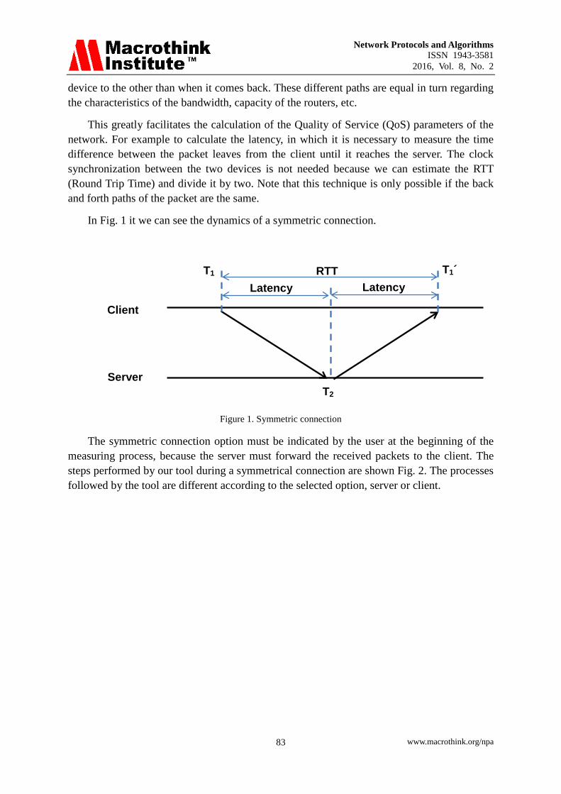
This greatly facilitates the calculation of the Quality of Service (QoS) parameters of the network. For example to calculate the latency, in which it is necessary to measure the time difference between the packet leaves from the client until it reaches the server. The clock synchronization between the two devices is not needed because we can estimate the RTT (Round Trip Time) and divide it by two. Note that this technique is only possible if the back and forth paths of the packet are the same.

In Fig. 1 it we can see the dynamics of a symmetric connection.

Client

Server

T1

T2

T1´ Latency Latency

RTT

Figure 1. Symmetric connection

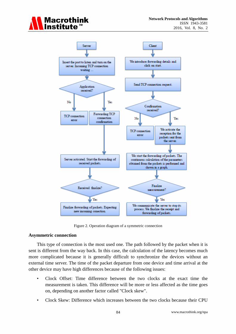
The symmetric connection option must be indicated by the user at the beginning of the measuring process, because the server must forward the received packets to the client. The steps performed by our tool during a symmetrical connection are shown Fig. 2. The processes followed by the tool are different according to the selected option, server or client.



2016, Vol. 8, No. 2

Figure 2. Operation diagram of a symmetric connection

Asymmetric connection

This type of connection is the most used one. The path followed by the packet when it is sent is different from the way back. In this case, the calculation of the latency becomes much more complicated because it is generally difficult to synchronize the devices without an external time server. The time of the packet departure from one device and time arrival at the other device may have high differences because of the following issues:

• Clock Offset: Time difference between the two clocks at the exact time the measurement is taken. This difference will be more or less affected as the time goes on, depending on another factor called "Clock skew".

• Clock Skew: Difference which increases between the two clocks because their CPU



2016, Vol. 8, No. 2

clock frequency difference. This generally happens in devices that are old and their clock battery has been affected over time, causing its depletion and obtaining a frequency difference between both clocks.

These differences between clocks must be overcome in order to obtain reliable measurements. There are synchronization systems between source and destination such as the use of GPS (Global-Positioning System) or NTP (Network Time Protocol), which provide synchronization between both clocks. It should be noted that both systems will be more or less accurate depending on the network traffic.

In our developed tool we do not estimate the OWD (One Way Delay) [20] in asymmetric connections, as we have seen that it is needed expensive equipment and it seems not to be as fast as required by our measure. Instead, we have relied on "Scheme to measure One-Way Delay Variation with detection and removal of clock skew" (OWDV) [21] by Makoto Aoki included in his doctoral thesis published in 2012 at the University of Electro-Communications Tokyo [22]. It is also included in several published papers [23] [24]. They include the theoretical system used to calculate the OWDV.

We use the following forwarding scheme between two devices. We take TS as the period used by the client to send consecutive packets and IPD (Inter Packet Delay) as the interval between the reception of consecutive packets. We estimate the AOWDV (Accumulative One-Way Delay Variation) as the sum of the difference between the total sending time of a burst of packets, measured from the first packet sent to the last one, and the total receipt time, measured from the first to the last received packet.

If we take measurements over a long period of time, we can express the AOWDV of a package, in particular, as is the sum of the difference between the IPD and the TS of each sent packet. It is defined in equation (1).

( 1 )

The value of AOWDV gives us an estimation of how the network is more or less congested. This value is incremented and decremented continuously due to the advancement and retardation of the packets in the network.

If we take the measurement for each packet, we can display the values in a chart with the average of these values per second, but only of the forwarding packet. This will provide a very useful value regarding the status of the network without using synchronization equipment.

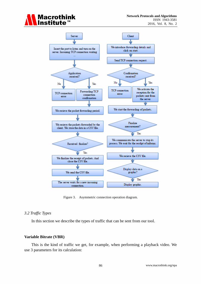
In figure 3, the actions carried out by the tool during a transmission in an asymmetric connection are described.



2016, Vol. 8, No. 2

Figure 3. Asymmetric connection operation diagram.

3.2 Traffic Types

In this section we describe the types of traffic that can be sent from our tool.

Variable Bitrate (VBR)

This is the kind of traffic we get, for example, when performing a playback video. We use 3 parameters for its calculation:



2016, Vol. 8, No. 2

• Frames per Second: 24, 25 or 29.97 fps.

• Maximum bitrate to achieve (Bytes).

• Minimum bitrate to achieve (Bytes).

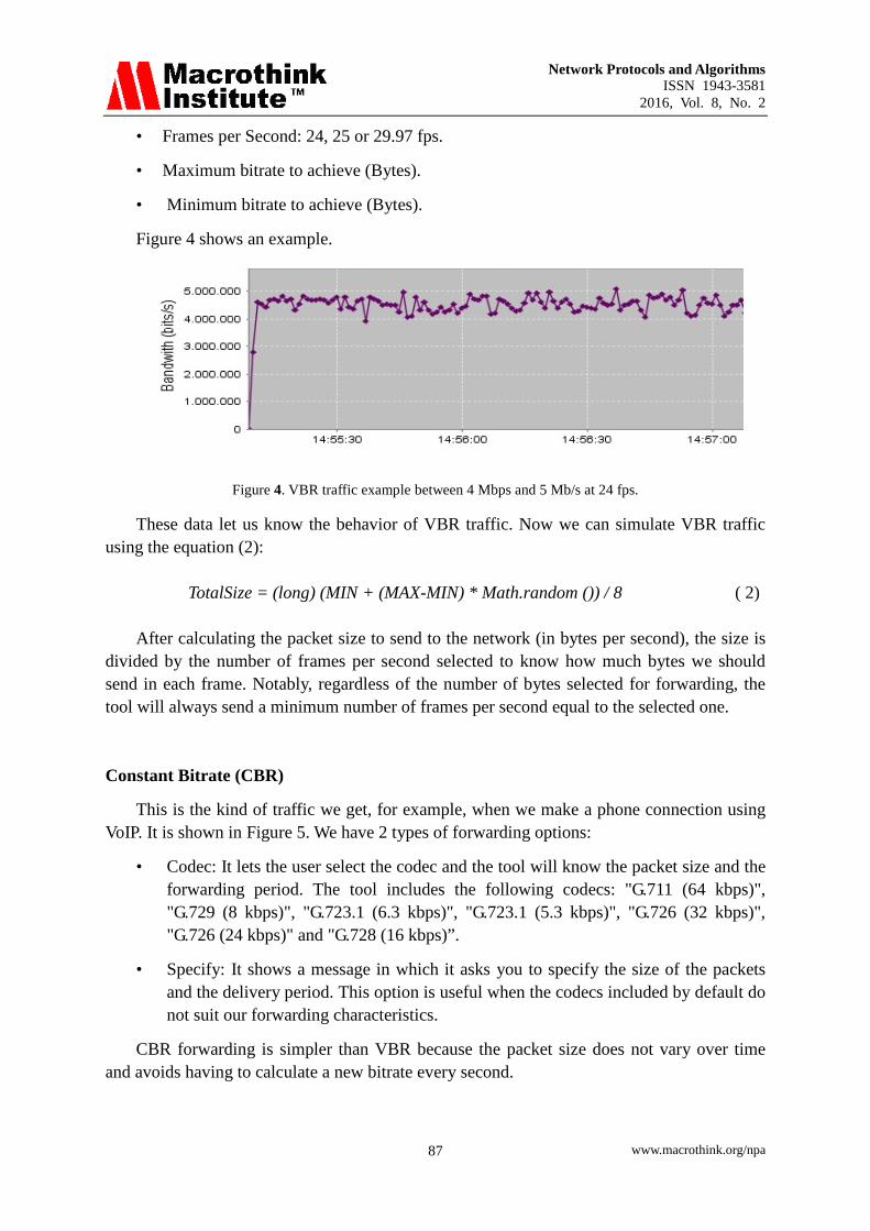
Figure 4 shows an example.

Figure 4. VBR traffic example between 4 Mbps and 5 Mb/s at 24 fps.

These data let us know the behavior of VBR traffic. Now we can simulate VBR traffic using the equation (2):

TotalSize = (long) (MIN + (MAX-MIN) * Math.random ()) / 8 ( 2)

After calculating the packet size to send to the network (in bytes per second), the size is divided by the number of frames per second selected to know how much bytes we should send in each frame. Notably, regardless of the number of bytes selected for forwarding, the tool will always send a minimum number of frames per second equal to the selected one.

Constant Bitrate (CBR)

This is the kind of traffic we get, for example, when we make a phone connection using VoIP. It is shown in Figure 5. We have 2 types of forwarding options:

• Codec: It lets the user select the codec and the tool will know the packet size and the forwarding period. The tool includes the following codecs: "G.711 (64 kbps)", "G.729 (8 kbps)", "G.723.1 (6.3 kbps)", "G.723.1 (5.3 kbps)", "G.726 (32 kbps)", "G.726 (24 kbps)" and "G.728 (16 kbps)”.

• Specify: It shows a message in which it asks you to specify the size of the packets and the delivery period. This option is useful when the codecs included by default do not suit our forwarding characteristics.

CBR forwarding is simpler than VBR because the packet size does not vary over time and avoids having to calculate a new bitrate every second.



2016, Vol. 8, No. 2

Time (hour:min:s)

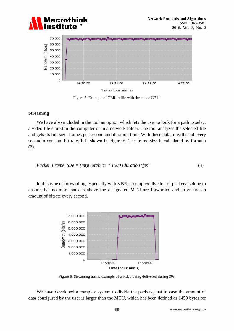
Figure 5. Example of CBR traffic with the codec G.711.

Streaming

We have also included in the tool an option which lets the user to look for a path to select a video file stored in the computer or in a network folder. The tool analyzes the selected file and gets its full size, frames per second and duration time. With these data, it will send every second a constant bit rate. It is shown in Figure 6. The frame size is calculated by formula (3).

Packet_Frame_Size = (int)(TotalSize * 1000 (duration*fps) (3)

In this type of forwarding, especially with VBR, a complex division of packets is done to ensure that no more packets above the designated MTU are forwarded and to ensure an amount of bitrate every second.

Time (hour:min:s)

Figure 6. Streaming traffic example of a video being delivered during 30s.

We have developed a complex system to divide the packets, just in case the amount of data configured by the user is larger than the MTU, which has been defined as 1450 bytes for



2016, Vol. 8, No. 2

our case. Our purpose was to not let the system take care of the fragmentation process in order to avoid possible latencies added by the system. The tool performs this task for all types of traffic available: VBR, CBR or Streaming.

3.3 Communication protocols used for measurements

Two communication protocols have been implemented in order to make and take measurements. The first one was designed by us. From now we are going to call it custom protocol. The protocol fields have been designed according to the test we wanted to do with the tool. The second protocol is RTP [25]. The application allows the user to select each one of them.

3.3.1 Custom header

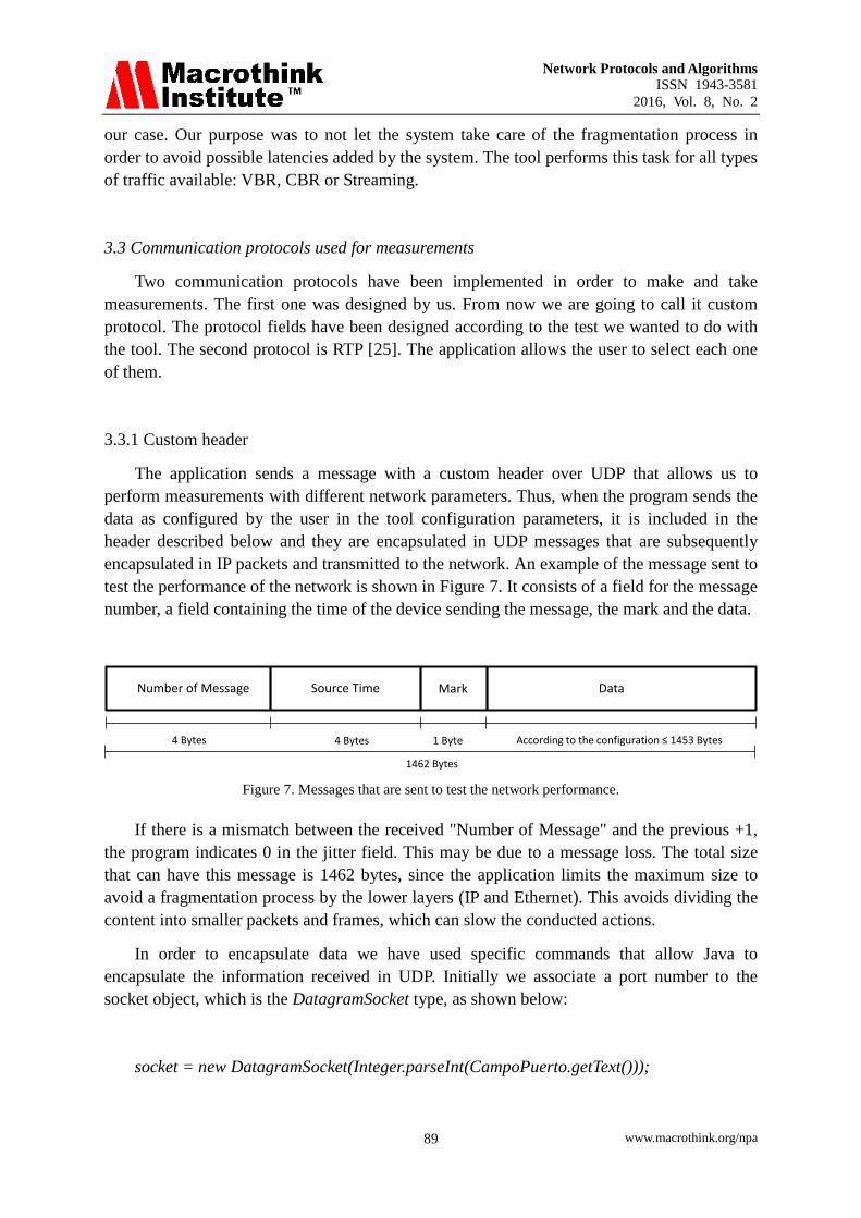
The application sends a message with a custom header over UDP that allows us to perform measurements with different network parameters. Thus, when the program sends the data as configured by the user in the tool configuration parameters, it is included in the header described below and they are encapsulated in UDP messages that are subsequently encapsulated in IP packets and transmitted to the network. An example of the message sent to test the performance of the network is shown in Figure 7. It consists of a field for the message number, a field containing the time of the device sending the message, the mark and the data.

Number of Message Source Time Data

4 Bytes 4 Bytes According to the configuration ≤ 1453 Bytes1 Byte

Mark

1462 Bytes Figure 7. Messages that are sent to test the network performance.

If there is a mismatch between the received "Number of Message" and the previous +1, the program indicates 0 in the jitter field. This may be due to a message loss. The total size that can have this message is 1462 bytes, since the application limits the maximum size to avoid a fragmentation process by the lower layers (IP and Ethernet). This avoids dividing the content into smaller packets and frames, which can slow the conducted actions.

In order to encapsulate data we have used specific commands that allow Java to encapsulate the information received in UDP. Initially we associate a port number to the socket object, which is the DatagramSocket type, as shown below:

socket = new DatagramSocket(Integer.parseInt(CampoPuerto.getText()));



2016, Vol. 8, No. 2

Then, we fill the header of the UDP message, which is the object. In order to do that, we use a class in which we create the message with the following code:

for (int i=0; i < 4; i++)

header[3-i] = new Integer(Packet_Number>>(8*i)).byteValue();

for (int i=0; i < 4; i++) header[7-i] = new Integer(TimeStamp>>(8*i)).byteValue();

header[8] = new Integer(mark).byteValue();

Then, we create an object called "sendpacket" to send it to the network. This message contains its length, destination IP address and destination port. This is shown below:

DatagramPacket sendpacket = new DatagramPacket(data,data.length,InetAddress.getByName(CampoIPField.getText()),Integer.parseInt(CampoPuertoField.getText()));

Jitter Calculation

To calculate the jitter, the tool records the time of arrival of each message and compares it to the time of the previous message, to do that it uses the "Number of Message" header fields. Next, we show the code used to estimate the jitter.

if ((paq.getsequencenumber() >= 2) && ((NumSeqAnterior == (paq.getsequencenumber()-1)))){ jitter = Math.abs( delay - PreviousDelay); } else { jitter = 0; }

Delay Calculation with NTP

To calculate the network delay, the tool uses the "Source Time" field of the message. It has the value of the arrival time of the message and subtracts both times to calculate the delay. In order to estimate it, it is necessary to have both computers completely synchronized. In our case, we installed on one computer an NTP (Network Time Protocol) server and on the other an NTP client. Using the following code, we obtain the arrival time of the message in milliseconds:



2016, Vol. 8, No. 2

ArrivalTime=Calendar.getInstance().getTimeInMillis();

Then we select the Source Time field:

SourceTime=Long.parseLong(tokens.nextToken());

And we calculate the difference to know the delay:

delay = (ArrivalTime - SourceTime);

Calculation of lost messages

For the calculation of the number of lost messages it is enough to count the number of messages received and compare this value with the "Message number" field of the header. The difference of these values will give the number of lost messages.

To calculate the percentage of lost messages, we simply divide the value of lost packets by the field "Message number" and multiply it by 100.

Calculation of Bandwidth

In order to calculate the bandwidth, the tool uses the UDP message length, with the "length" function, because it provides the number of bytes of the packet. Then, it multiplies it by 8 in order to represent it in bits.

3.3.2 RTP header

The tool has the RTP (Real Time Protocol) header implemented by default, but it is designed in a modular way in order to let the developers add more headers easily by making small changes in the source code.

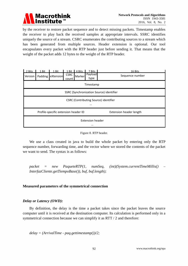
As we know the RTP header has the fields shown in Figure 8. It follows the header defined in [25]. The fields in the header are next ones. Version indicates the version of the protocol (currently version=2). Padding is used to indicate whether there are extra padding bytes at the end of the RTP packet or not. Extension indicates presence of an extension header between standard header and payload data. CSRC count provides the number of CSRC identifiers. Marker is defined by a profile and used at the application level. Payload type indicates the format of the payload and determines how the application should be interpreted. The sequence number is incremented by one every time a RTP data packet is sent. It is used



2016, Vol. 8, No. 2

by the receiver to restore packet sequence and to detect missing packets. Timestamp enables the receiver to play back the received samples at appropriate intervals. SSRC identifies uniquely the source of a stream. CSRC enumerates the contributing sources to a stream which has been generated from multiple sources. Header extension is optional. Our tool encapsulates every packet with the RTP header just before sending it. That means that the weight of the packet adds 12 bytes to the weight of the RTP header.

Version2 Bits 1 Bit 1 Bit 1 Bit

Padding eXtension CSRC count

MarkerPayload

type

4 Bits 7 BitsSequence number

16 Bits

Timestamp

SSRC (Synchronization Source) identifier

CSRC (Contributing Source) identifier…

Extension header…

Profile-specific extension header ID Extension header length

Figure 8. RTP header.

We use a class created in java to build the whole packet by entering only the RTP sequence number, forwarding time, and the vector where we stored the contents of the packet we want to send. The syntax is as follows:

packet = new PaqueteRTP(1, numSeq, (int)(System.currentTimeMillis() – InterfazCliente.getTiempoBase()), buf, buf.length);

Measured parameters of the symmetrical connection

Delay or Latency (OWD):

By definition, the delay is the time a packet takes since the packet leaves the source computer until it is received at the destination computer. Its calculation is performed only in a symmetrical connection because we can simplify it as RTT / 2 and therefore:

delay = (ArrivalTime - paq.gettimestamp())/2;



2016, Vol. 8, No. 2

Jitter

For the jitter calculation, as it has been defined before, it is the difference between a packet delay and the delay of the packet received previously. Therefore we use the above syntax for calculating the delay and add some details:

if((paq.getsequencenumber() >= 2) && (NumSeqAnterior == (paq.getsequencenumber() - 1) || ((NumSeqAnterior - 65535) == paq.getsequencenumber()))){ jitter = Math.abs( delay - PreviousDelay ;} else{ jitter = 0;}

In order to measure the jitter, we should start from the second package, and made a couple of verifications. It should meet at least one of next two options in order to estimate the jitter:

1. The sequence number of the current packet minus one is equal to the sequence number of the previous packet.

2. The sequence number of the current packet is equal to the previous sequence number minus 65535. It means that we have completed the packet counter and we restart the counter.

Lost packets

For the calculation of lost packets we use a counter that counts the packets received and we compare it to the sequence number of the packet. It is noteworthy that, as the number of the packet sequence is cyclical, we establish a mechanism that can count the amount of times the sequence number of the packets has restarted, so we can make the calculation of lost packets correctly. Below is presented the code used for the calculation:

LostPackets = paq.getsequencenumber() + (ContadorNumSeq * 65535) – ReceivedPackets;

We also calculate the percentage of lost packets which is only a small modification of the above code:

%LostPackets = paq.getsequencenumber() + (ContadorNumSeq * 65535) – ReceivedPackets /paq.getsequencenumber())*100;



2016, Vol. 8, No. 2

Measured parameters of asymmetric connection

The most important parameter in asymmetric connection is the AOWDV. It is the aggregated value of the time variation of the period of two consecutive packets received at the destination device. This measure can be very useful to see how the packets behave through a network where there could be different delays.

In order to estimate it we perform several processes:

1. Upon receipt of each packet, we calculate the OWDV with the code shown below. It is applied to the packet received after the packet with the marker activated. The marker indicates the last packet of a burst sent in a frame.

OneWayDelayVariation=ArrivalTime – PreviousArrivalTime – period;

If the previous received packet does not have an activated marker, we use the following code:

OneWayDelayVariation= ArrivalTime – PreviousArrivalTime;

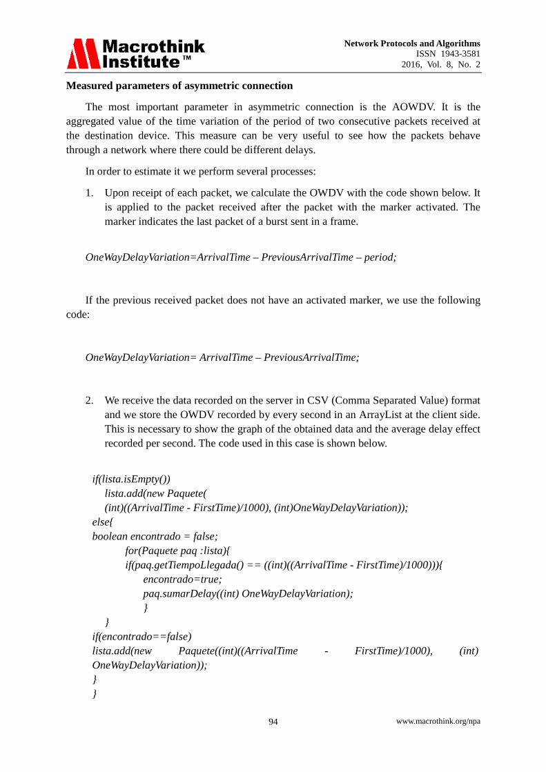
2. We receive the data recorded on the server in CSV (Comma Separated Value) format and we store the OWDV recorded by every second in an ArrayList at the client side. This is necessary to show the graph of the obtained data and the average delay effect recorded per second. The code used in this case is shown below.

if(lista.isEmpty())

lista.add(new Paquete( (int)((ArrivalTime - FirstTime)/1000), (int)OneWayDelayVariation));

else{ boolean encontrado = false; for(Paquete paq :lista){ if(paq.getTiempoLlegada() == ((int)((ArrivalTime - FirstTime)/1000))){ encontrado=true; paq.sumarDelay((int) OneWayDelayVariation); } } if(encontrado==false) lista.add(new Paquete((int)((ArrivalTime - FirstTime)/1000), (int) OneWayDelayVariation)); } }



2016, Vol. 8, No. 2

This code allows the tool to gather the average OWDV per second in order to display a graph on the client. Figure 9 shows an example of the obtained graph.

Time (s)

Figure 9. OWDV graphic.

Format of the report stored on disk

The tool allows saving the measured parameters in the CSV format files. It is basically a text file in which each value is separated by commas. It is widely recognized file and it can be opened with programs for processing spreadsheets such as Microsoft Excel. Such programs organize the data in rows and columns which let us obtain graphs easily.

4. Graphic interface of the test tool

We have developed an application that allows the user to choose to be Client or Server. The client allows choosing the type of traffic sent to the server (audio or video) and the server forwards that traffic to the client. In the client side, the jitter, delay, lost messages, and percentage of lost messages, bandwidth, etc., are calculated and recorded. The client displays all these data per second in a very intuitive and easy to use graphical interface. In addition, it shows the last 20 received packets in a table.

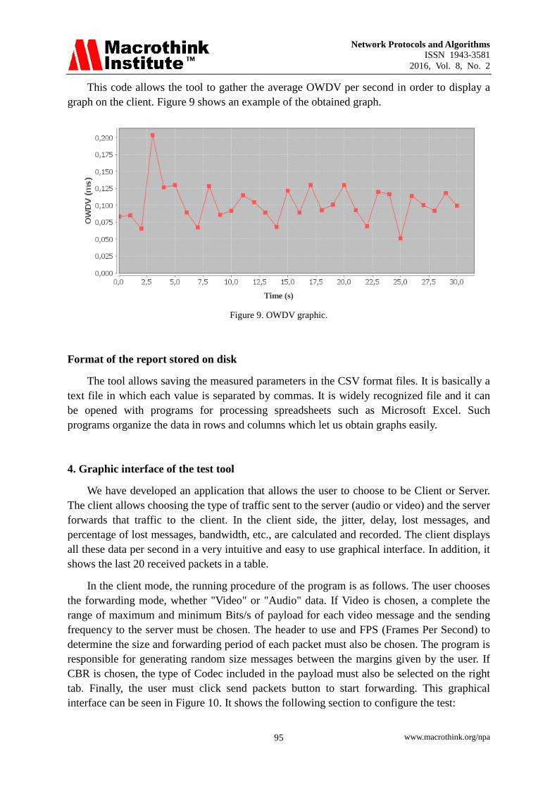
In the client mode, the running procedure of the program is as follows. The user chooses the forwarding mode, whether "Video" or "Audio" data. If Video is chosen, a complete the range of maximum and minimum Bits/s of payload for each video message and the sending frequency to the server must be chosen. The header to use and FPS (Frames Per Second) to determine the size and forwarding period of each packet must also be chosen. The program is responsible for generating random size messages between the margins given by the user. If CBR is chosen, the type of Codec included in the payload must also be selected on the right tab. Finally, the user must click send packets button to start forwarding. This graphical interface can be seen in Figure 10. It shows the following section to configure the test:



2016, Vol. 8, No. 2

• A section to choose the type of connection: symmetrical or asymmetrical.

• A section to choose the type of traffic to be sent: 1) VBR (Variable Bitrate) traffic type option which allows the selection of the header to use for VBR (it may be RTP, or the one designed by us [26]), the selection of the frames per second to use and the maximum and minimum bitrate limits (in bits per second). 2) CBR (Constant Bitrate) traffic type option, which allows the selection of the header to use for CBR (it may be RTP, or the designed by us [26]), the selection of the codec to use including an option where the user can specify the size of the packet and forwarding period. 3) Streaming traffic type option, where the user must choose the path of the file for its delivery.

• A section where the user provides the information about the destination IP address and destination port.

• Start forwarding button and end forwarding button

• Window that displays the messages about the status of the tool.

Figure 10. Client mode configuration.

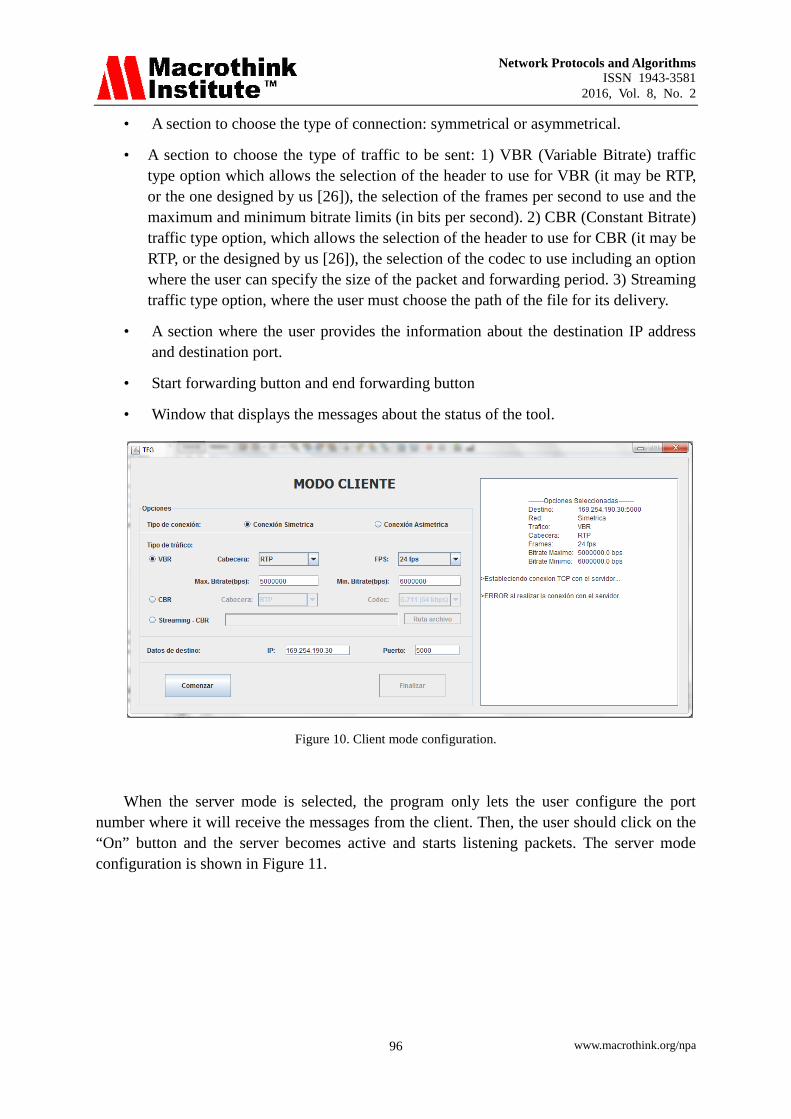
When the server mode is selected, the program only lets the user configure the port number where it will receive the messages from the client. Then, the user should click on the “On” button and the server becomes active and starts listening packets. The server mode configuration is shown in Figure 11.



2016, Vol. 8, No. 2

Figure 11. Server mode configuration.

5. Performance Test

In order to test the developed tool, we performed several tests. Although the tool can be easily used just to test the network convergence time using routing protocols [27] or to test the video delivery in wireless local area networks [28], we will focus our test on the QoS parameters.

5.1 Test in a local network

First, we tested the tool between 2 computers belonging to the same IP network. They were connected to the same switch. Both computers used FastEthernet.

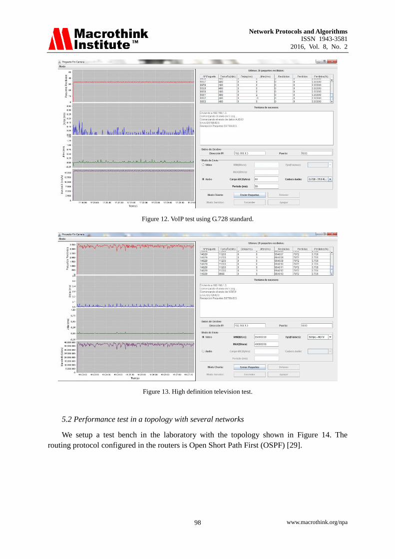
Figure 12 shows the parameters obtained when the client sends VoIP traffic using the G728 standard. We can observe that the used bandwidth is practically constant, and we do not observe lost packets. The jitter and delay values are very low, because they are connected to the same switch, but they are appreciable.

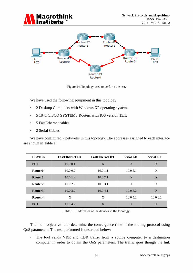
Figure 13 shows the results obtained when high-definition video is sent between both computers. In this case, both the bandwidth and the number of received packets have risen considerably. However, both the jitter and the delay are still low.



2016, Vol. 8, No. 2

Figure 12. VoIP test using G.728 standard.

Figure 13. High definition television test.

5.2 Performance test in a topology with several networks

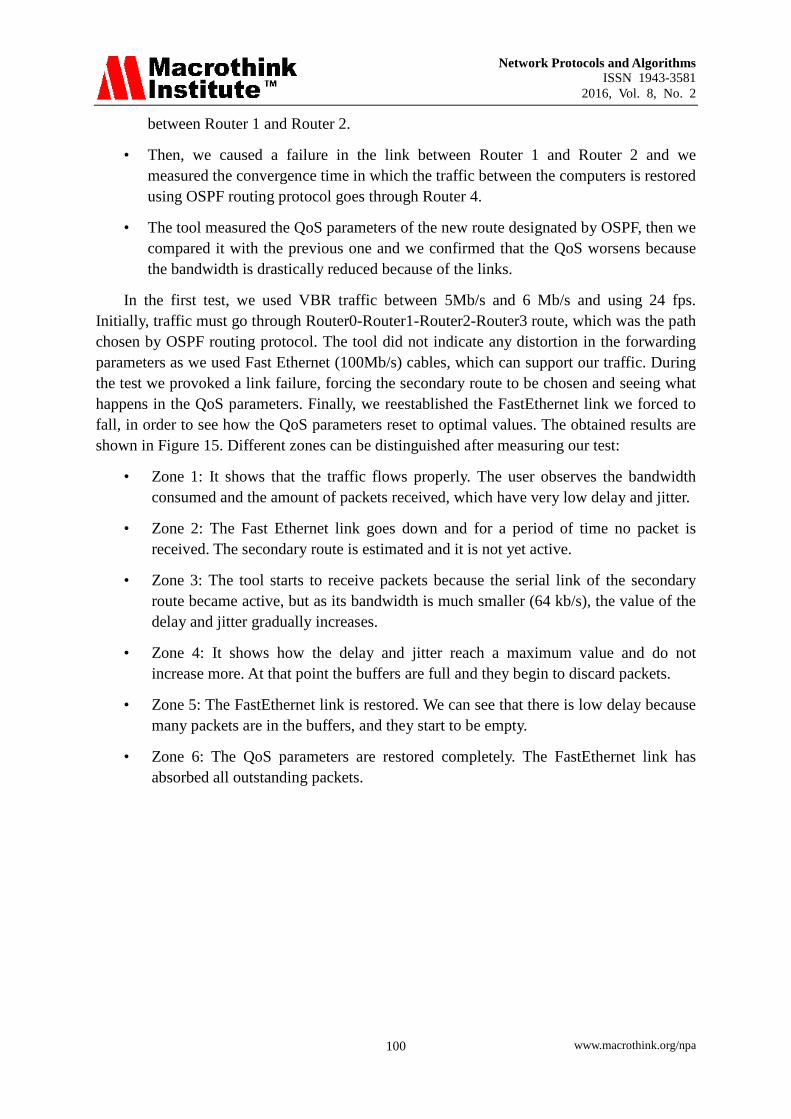
We setup a test bench in the laboratory with the topology shown in Figure 14. The routing protocol configured in the routers is Open Short Path First (OSPF) [29].



2016, Vol. 8, No. 2

Figure 14. Topology used to perform the test.

We have used the following equipment in this topology:

• 2 Desktop Computers with Windows XP operating system.

• 5 1841 CISCO SYSTEMS Routers with IOS version 15.1.

• 5 FastEthernet cables.

• 2 Serial Cables.

We have configured 7 networks in this topology. The addresses assigned to each interface are shown in Table 1.

DEVICE FastEthernet 0/0 FastEthernet 0/1 Serial 0/0 Serial 0/1

PC0 10.0.0.1 X X X

Router0 10.0.0.2 10.0.1.1 10.0.5.1 X

Router1 10.0.1.2 10.0.2.1 X X

Router2 10.0.2.2 10.0.3.1 X X

Router3 10.0.3.2 10.0.4.1 10.0.6.2 X

Router4 X X 10.0.5.2 10.0.6.1

PC1 10.0.4.2 X X X

Table 1. IP addresses of the devices in the topology.

The main objective is to determine the convergence time of the routing protocol using QoS parameters. The test performed is described below:

• The tool sends VBR and CBR traffic from a source computer to a destination computer in order to obtain the QoS parameters. The traffic goes though the link



2016, Vol. 8, No. 2

between Router 1 and Router 2.

• Then, we caused a failure in the link between Router 1 and Router 2 and we measured the convergence time in which the traffic between the computers is restored using OSPF routing protocol goes through Router 4.

• The tool measured the QoS parameters of the new route designated by OSPF, then we compared it with the previous one and we confirmed that the QoS worsens because the bandwidth is drastically reduced because of the links.

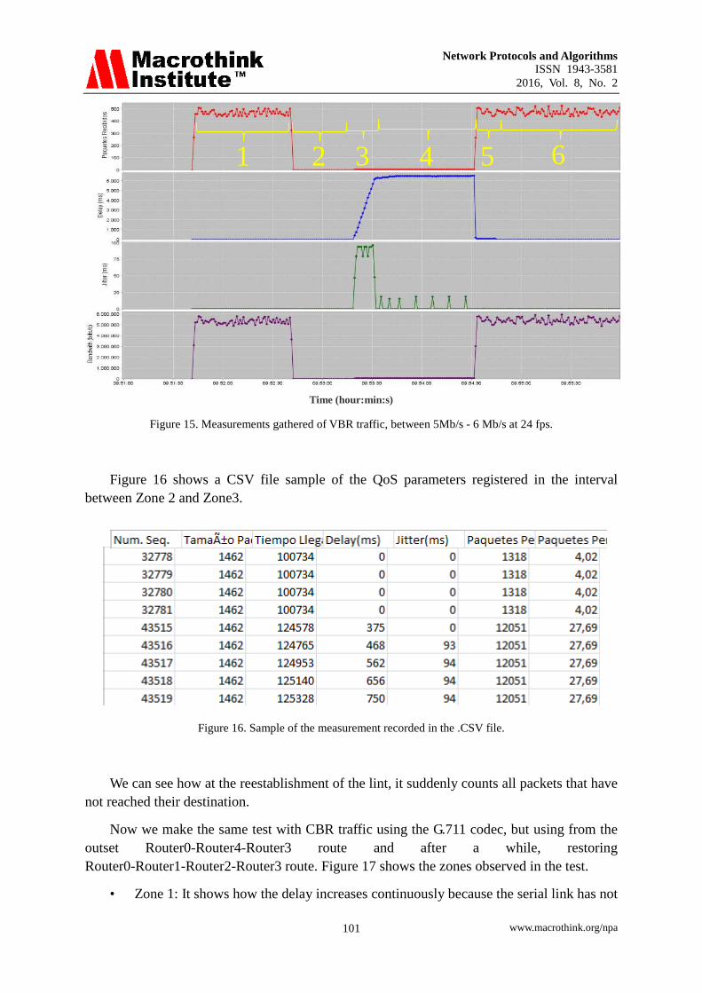
In the first test, we used VBR traffic between 5Mb/s and 6 Mb/s and using 24 fps. Initially, traffic must go through Router0-Router1-Router2-Router3 route, which was the path chosen by OSPF routing protocol. The tool did not indicate any distortion in the forwarding parameters as we used Fast Ethernet (100Mb/s) cables, which can support our traffic. During the test we provoked a link failure, forcing the secondary route to be chosen and seeing what happens in the QoS parameters. Finally, we reestablished the FastEthernet link we forced to fall, in order to see how the QoS parameters reset to optimal values. The obtained results are shown in Figure 15. Different zones can be distinguished after measuring our test:

• Zone 1: It shows that the traffic flows properly. The user observes the bandwidth consumed and the amount of packets received, which have very low delay and jitter.

• Zone 2: The Fast Ethernet link goes down and for a period of time no packet is received. The secondary route is estimated and it is not yet active.

• Zone 3: The tool starts to receive packets because the serial link of the secondary route became active, but as its bandwidth is much smaller (64 kb/s), the value of the delay and jitter gradually increases.

• Zone 4: It shows how the delay and jitter reach a maximum value and do not increase more. At that point the buffers are full and they begin to discard packets.

• Zone 5: The FastEthernet link is restored. We can see that there is low delay because many packets are in the buffers, and they start to be empty.

• Zone 6: The QoS parameters are restored completely. The FastEthernet link has absorbed all outstanding packets.



2016, Vol. 8, No. 2

Time (hour:min:s)

Figure 15. Measurements gathered of VBR traffic, between 5Mb/s - 6 Mb/s at 24 fps.

Figure 16 shows a CSV file sample of the QoS parameters registered in the interval between Zone 2 and Zone3.

Figure 16. Sample of the measurement recorded in the .CSV file.

We can see how at the reestablishment of the lint, it suddenly counts all packets that have not reached their destination.

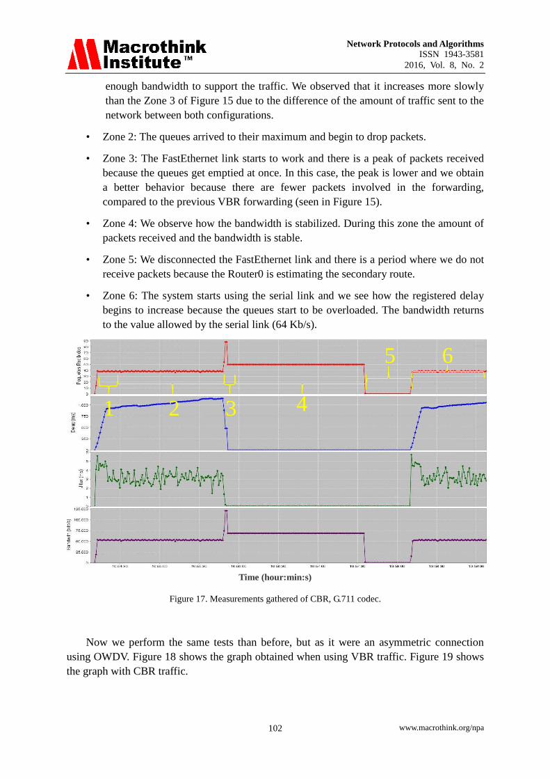
Now we make the same test with CBR traffic using the G.711 codec, but using from the outset Router0-Router4-Router3 route and after a while, restoring Router0-Router1-Router2-Router3 route. Figure 17 shows the zones observed in the test.

• Zone 1: It shows how the delay increases continuously because the serial link has not

1 4 3 2 5 6



2016, Vol. 8, No. 2

enough bandwidth to support the traffic. We observed that it increases more slowly than the Zone 3 of Figure 15 due to the difference of the amount of traffic sent to the network between both configurations.

• Zone 2: The queues arrived to their maximum and begin to drop packets.

• Zone 3: The FastEthernet link starts to work and there is a peak of packets received because the queues get emptied at once. In this case, the peak is lower and we obtain a better behavior because there are fewer packets involved in the forwarding, compared to the previous VBR forwarding (seen in Figure 15).

• Zone 4: We observe how the bandwidth is stabilized. During this zone the amount of packets received and the bandwidth is stable.

• Zone 5: We disconnected the FastEthernet link and there is a period where we do not receive packets because the Router0 is estimating the secondary route.

• Zone 6: The system starts using the serial link and we see how the registered delay begins to increase because the queues start to be overloaded. The bandwidth returns to the value allowed by the serial link (64 Kb/s).

Time (hour:min:s)

Figure 17. Measurements gathered of CBR, G.711 codec.

Now we perform the same tests than before, but as it were an asymmetric connection using OWDV. Figure 18 shows the graph obtained when using VBR traffic. Figure 19 shows the graph with CBR traffic.

2 4

6 5

1 3



2016, Vol. 8, No. 2

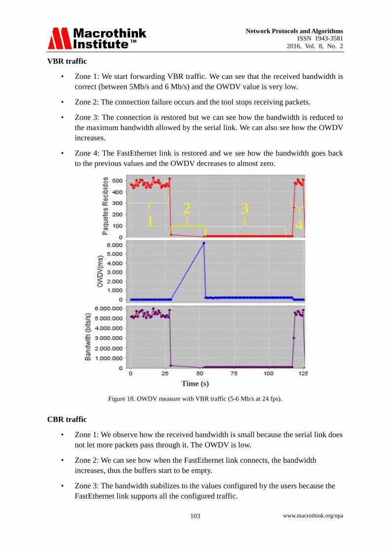
VBR traffic

• Zone 1: We start forwarding VBR traffic. We can see that the received bandwidth is correct (between 5Mb/s and 6 Mb/s) and the OWDV value is very low.

• Zone 2: The connection failure occurs and the tool stops receiving packets.

• Zone 3: The connection is restored but we can see how the bandwidth is reduced to the maximum bandwidth allowed by the serial link. We can also see how the OWDV increases.

• Zone 4: The FastEthernet link is restored and we see how the bandwidth goes back to the previous values and the OWDV decreases to almost zero.

Time (s)

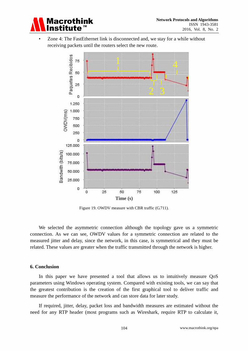
Figure 18. OWDV measure with VBR traffic (5-6 Mb/s at 24 fps). CBR traffic

• Zone 1: We observe how the received bandwidth is small because the serial link does not let more packets pass through it. The OWDV is low.

• Zone 2: We can see how when the FastEthernet link connects, the bandwidth increases, thus the buffers start to be empty.

• Zone 3: The bandwidth stabilizes to the values configured by the users because the FastEthernet link supports all the configured traffic.

1 2 3

4



2016, Vol. 8, No. 2

• Zone 4: The FastEthernet link is disconnected and, we stay for a while without receiving packets until the routers select the new route.

Time (s)

Figure 19. OWDV measure with CBR traffic (G.711).

We selected the asymmetric connection although the topology gave us a symmetric connection. As we can see, OWDV values for a symmetric connection are related to the measured jitter and delay, since the network, in this case, is symmetrical and they must be related. These values are greater when the traffic transmitted through the network is higher.

6. Conclusion

In this paper we have presented a tool that allows us to intuitively measure QoS parameters using Windows operating system. Compared with existing tools, we can say that the greatest contribution is the creation of the first graphical tool to deliver traffic and measure the performance of the network and can store data for later study.

If required, jitter, delay, packet loss and bandwidth measures are estimated without the need for any RTP header (most programs such as Wireshark, require RTP to calculate it,

1

2 3

4



2016, Vol. 8, No. 2

otherwise, they are not able to do it).

Future works are focused on checking the reliability, advantages and disadvantages of our tool by comparing it with existing tools. Furthermore, we will use it to test the performance of the most common routing protocols and to test other transport and application protocols.

Acknowledgements

This work has been supported by the “Ministerio de Economía y Competitividad”, through the “Convocatoria 2014. Proyectos I+D - Programa Estatal de Investigación Científica y Técnica de Excelencia” in the “Subprograma Estatal de Generación de Conocimiento”, project TIN2014-57991-C3-1-P and the “programa para la Formación de Personal Investigador – (FPI-2015-S2-884)” by the “Universitat Politècnica de València”.

References

[1] IBM Corporation, "IBM Study Related to the NEP Industry", 2007. Available at: http://www-935.ibm.com/services/us/gbs/bus/pdf/g510-7870-01-nep.pdf

[2] J. Postel, Internet Control Message Protocol, RFC 792, September 1981. Available at http://www.ietf.org/rfc/rfc0792.txt

[3] J. Case, M. Fedor, M. Schoffstall, J. Davin, A Simple Network Management Protocol (SNMP), RFC 1157. May 1990. Available at: http://tools.ietf.org/html/rfc1157

[4] S. Waldbusser, Remote Network Monitoring Management Information Base, RFC 2819. May 2000. Available at: http://tools.ietf.org/html/rfc2819

[5] S. Waldbusser, Remote Network Monitoring Management Information Base Version 2 using SMIv2. RFC 4502. May 2006. Available at: http://tools.ietf.org/html/rfc4502

[6] SendIP. Available at: http://www.earth.li/projectpurple/progs/sendip.html [7] W. Feng, A. Goel, A. Bezzaz, W. Feng, J. Walpole, "TCPivo: A High-Performance Packet

Replay Engine", ACM SIGCOMM 2003 Workshop on Models, Methods, and Tools for Reproducible Network Research (MoMeTools), August 2003. http://dx.doi.org/10.1145/944773.944783

[8] Rude&Crude. Available at: http://rude.sourceforge.net/ [9] Scapy Project. Available at: http://www.secdev.org/projects/scapy/doc/index.html [10] Daniel Turrull Torrents, Open Source Traffic Analyzer. Master of Science Thesis.

Stockholm, Sweden. June, 2010. Available at: http://people.kth.se/~danieltt/pktgen/docs/DanielTurull-thesis.pdf

[11] Joel Sommers, Hyungsuk Kim and Paul Barford, Harpoon: a flow-level traffic generator for router and network tests, ACM SIGMETRICS Performance Evaluation Review, Volume 32 Issue 1, June 2004. Pp. 392-392. http://dx.doi.org/10.1145/1012888.1005733

[12] Nemesis. Available at: http://nemesis.sourceforge.net/ [13] Packet Excalibur. Available at: http://freecode.com/projects/packetexcalibur [14] PackETH. Available at: http://packeth.sourceforge.net/packeth/Home.html [15] ISIC -- IP Stack Integrity Checker. Available at: http://isic.sourceforge.net/



2016, Vol. 8, No. 2

[16] Netperf Homepage http://www.netperf.org/netperf/ [17] NetSpec: A Tool for Network Experimentation and Measurement. Available at:

http://www.ittc.ku.edu/netspec/ [18] Bit-Twist website. Available at: http://bittwist.sourceforge.net/ [19] A. Dainotti, A. Botta, A. Pescapè, "A tool for the generation of realistic network workload

for emerging networking scenarios", Computer Networks, 2012, Volume 56, Issue 15, pp 3531-3547. http://dx.doi.org/10.1016/j.comnet.2012.02.019

[20] Laura Tomaciello, Luca De Vito, Sergio Rapuano, One-Way Delay Measurement: State of Art, 2006 IEEE Instrumentation and Measurement Technology Conference, Sorrento, Italy, 24-27 April 2006. http://dx.doi.org/10.1109/IMTC.2006.328401

[21] M. Aoki and E. Oki, “A Scheme to Estimate One-way Delay Variations for Diagnosing Network Traffic Conditions”, Cyber Journals: Multidisciplinary Journals in Science and Technology, Journal of Selected Areas in Telecommunications (JSAT), August Edition, 2011.

[22] Makoto Aoki, “Estimation on Quality of Service for real-Time Communications in IP Networks” University of Electro-Communications of Japan, March 2012. Available at:

http://ir.lib.uec.ac.jp/infolib/user_contents/9000000635/9000000635.pdf [23] M. Aoki and E. Oki, “Estimating ADSL Link Capacity by Measuring RTT of Different

Length Packets,” IEICE Letter, Vol.E94-B, No.12, Dec. 2011. [24] M. Aoki, R. Rojas-Cessa, and E. Oki, “Measurement Scheme for One-way Delay

Variation with Detection and Removal of Clock Skew,” ETRI Journal, Vol.32, No.6, pp. 854-862, Dec. 2010. http://dx.doi.org/10.4218/etrij.10.0109.0611

[25] H. Schulzrinne, S. Casner, R. Frederick, V. Jacobson, RTP: A Transport Protocol for Real-Time Applications, RFC 3550. July 2003, Available at: https://www.ietf.org/rfc/rfc3550.txt

[26]Carlos Barambones, David Pascual, Juan R. Diaz, Jaime Lloret, Una Nueva Herramienta para Testear el Rendimiento de una Red IP, XI Jornadas de Ingeniería Telemática (JITEL 2013), Granada (Spain), October 28-30, 2013

[27]S. Sendra, P.A. Fernández, M.A. Quilez, J. Lloret, Study and performance of interior gateway IP routing protocols, Network Protocols and Algorithms 2 (4), 88-117. 2011. http://dx.doi.org/10.5296/npa.v2i4.547

[28]M. Atenas, S. Sendra, M .Garcia, J. Lloret, IPTV Performance in IEEE 802.11 n WLANs, 2010 IEEE Globecom Workshops, Miami, USA. 6-10 Dec. 2010. Pp. 929-933. http://dx.doi.org/10.1109/GLOCOMW.2010.5700461

[28]J. Moy, OSPF Version 2 (RFC 2328). April 1998. Available at: https://www.ietf.org/rfc/rfc2328.txt

Copyright Disclaimer

Copyright reserved by the author(s).

This article is an open-access article distributed under the terms and conditions of the Creative Commons Attribution license (http://creativecommons.org/licenses/by/3.0/).


a new tool to test the ip network performance

Documents