a non-equilibrium model for soil heating and moisture transport … · 2016-08-18 · a...
TRANSCRIPT
Geosci. Model Dev., 8, 3659–3680, 2015
www.geosci-model-dev.net/8/3659/2015/
doi:10.5194/gmd-8-3659-2015
© Author(s) 2015. CC Attribution 3.0 License.
A non-equilibrium model for soil heating and moisture transport
during extreme surface heating: the soil (heat–moisture–vapor)
HMV-Model Version 1
W. J. Massman
USDA Forest Service, Rocky Mountain Research Station, 240 West Prospect, Fort Collins, CO 80526, USA
Correspondence to: W. J. Massman ([email protected])
Received: 4 February 2015 – Published in Geosci. Model Dev. Discuss.: 6 March 2015
Revised: 3 September 2015 – Accepted: 16 October 2015 – Published: 6 November 2015
Abstract. Increased use of prescribed fire by land managers
and the increasing likelihood of wildfires due to climate
change require an improved modeling capability of extreme
heating of soils during fires. This issue is addressed here by
developing and testing the soil (heat–moisture–vapor) HMV-
model, a 1-D (one-dimensional) non-equilibrium (liquid–
vapor phase change) model of soil evaporation that simu-
lates the coupled simultaneous transport of heat, soil mois-
ture, and water vapor. This model is intended for use with
surface forcing ranging from daily solar cycles to extreme
conditions encountered during fires. It employs a linearized
Crank–Nicolson scheme for the conservation equations of
energy and mass and its performance is evaluated against
dynamic soil temperature and moisture observations, which
were obtained during laboratory experiments on soil samples
exposed to surface heat fluxes ranging between 10 000 and
50 000 W m−2. The Hertz–Knudsen equation is the basis for
constructing the model’s non-equilibrium evaporative source
term. Some unusual aspects of the model that were found to
be extremely important to the model’s performance include
(1) a dynamic (temperature and moisture potential depen-
dent) condensation coefficient associated with the evapora-
tive source term, (2) an infrared radiation component to the
soil’s thermal conductivity, and (3) a dynamic residual soil
moisture. This last term, which is parameterized as a function
of temperature and soil water potential, is incorporated into
the water retention curve and hydraulic conductivity func-
tions in order to improve the model’s ability to capture the
evaporative dynamics of the strongly bound soil moisture,
which requires temperatures well beyond 150 ◦C to fully
evaporate. The model also includes film flow, although this
phenomenon did not contribute much to the model’s overall
performance. In general, the model simulates the laboratory-
observed temperature dynamics quite well, but is less pre-
cise (but still good) at capturing the moisture dynamics. The
model emulates the observed increase in soil moisture ahead
of the drying front and the hiatus in the soil temperature rise
during the strongly evaporative stage of drying. It also cap-
tures the observed rapid evaporation of soil moisture that oc-
curs at relatively low temperatures (50–90 ◦C), and can pro-
vide quite accurate predictions of the total amount of soil
moisture evaporated during the laboratory experiments. The
model’s solution for water vapor density (and vapor pres-
sure), which can exceed 1 standard atmosphere, cannot be ex-
perimentally verified, but they are supported by results from
(earlier and very different) models developed for somewhat
different purposes and for different porous media. Overall,
this non-equilibrium model provides a much more physically
realistic simulation over a previous equilibrium model de-
veloped for the same purpose. Current model performance
strongly suggests that it is now ready for testing under field
conditions.
1 Introduction
Since the development of the theory of Philip and de Vries
(PdV model) almost 60 years ago (Philip and de Vries, 1957;
de Vries, 1958), virtually all models of evaporation and con-
densation in unsaturated soils have assumed that soil water
vapor at any particular depth into the soil is in equilibrium
with the liquid soil water (or soil moisture) at the same depth.
(Note that such soil evaporation models also assume ther-
mal equilibrium, so that at any given depth the mineral soil,
Published by Copernicus Publications on behalf of the European Geosciences Union.

3660 W. J. Massman: The HMV model version 1
the soil moisture, and the soil air and water vapor within the
pore space are also at the same temperature.) In essence, this
local equilibrium assumption means that whenever the soil
moisture changes phase it does so instantaneously. This as-
sumption is quite apropos for its original application, which
was to describe the coupled heat and moisture transport in
soils (and soil evaporation in particular) under environmental
forcings associated with the daily and seasonal variations in
radiation, temperature, precipitation, etc. (e.g., Milly, 1982;
Novak, 2010; Smits et al., 2011). Under these conditions,
assuming local equilibrium is reasonable because the time
required to achieve equilibrium after a change of phase is
“instantaneous” (short) relative to the timescale associated
with normal environmental forcing. The great benefit to the
equilibrium assumption is that for modeling purposes it is a
significant simplification to the equations that describe heat
and moisture flow in soils because it eliminates the need
to include soil water vapor density, ρv, as an independent
model variable. More formally, under equilibrium ρv is di-
rectly equated to the equilibrium vapor density, a function
only of local soil temperature and soil water content (or more
specifically the soil water potential).
Subsequent to the development of the original PdV model
the equilibrium assumption has also been incorporated into
models of heat and moisture transport (evaporation and con-
densation) in soils and other porous media under more ex-
treme forcings associated with high temperatures and heat
fluxes. For example, it has been applied to (i) soils dur-
ing wildfires and prescribed burns (Aston and Gill, 1976;
Campbell et al., 1995; Durany et al., 2010; Massman, 2012),
(ii) drying of wood (Whitaker, 1977; di Blasi, 1997), (iii) dry-
ing and fracturing of concrete under high temperatures
(Dayan, 1982; Dal Pont et al., 2011), (iv) high temperature
sand–water–steam systems (e.g., Udell, 1983; Bridge et al.,
2003), and (v) evaporation of wet porous thermal barriers un-
der high heat fluxes (Costa et al., 2008).
Although the PdV model and the equilibrium assumption
have certainly led to many insights into moisture and va-
por transport and evaporation in porous media, they have,
nonetheless, yielded somewhat disappointing simulations of
the coupled soil moisture dynamics during fires (see Mass-
man, 2012, for further details and general modeling review).
Possibly the most interesting of these modeling “disappoint-
ments” is the soil/fire-heating model of Massman (2012),
who found that as the soil moisture evaporated it just re-
condensed and accumulated ahead of the dry zone; conse-
quently, no water actually escaped the soil at all, which, to
say the least, seems physically implausible. He further traced
the cause of this anomalous behavior to the inapplicability
of the equilibrium evaporation assumption, which allowed
the soil vapor gradient behind the drying front to become
so small that the soil vapor could not escape (diffuse) out
of the soil. Moreover, more fundamentally, the calculated va-
por and its attendant gradient became largely meaningless
because it is impossible for water vapor to be in equilibrium
with liquid water if there is no liquid water. Of course, such
extremely dry conditions are just about guaranteed during
soil heating events like fires. Novak (2012) also recognized
the inapplicability of the equilibrium assumption for very
dry soils, but under more normal environmental forcing. On
the other hand, even under normal (and much less extreme)
soil moisture conditions both Smits et al. (2011) and Oue-
draogo et al. (2013) suggest that non-equilibrium formula-
tions of soil evaporation may actually improve model perfor-
mance, which implies that the non-equilibrium assumption
may really be a more appropriate description for soil evap-
oration and condensation than the equilibrium assumption.
The present study is intended to provide the first test of the
non-equilibrium hypothesis during extreme conditions.
Specifically, the present study develops and evaluates a
non-equilibrium (liquid–vapor phase change) model for sim-
ulating coupled heat, moisture, and water vapor transport
during extreme heating events. It also assumes thermal equi-
librium between the soil solids, liquid, and vapor. It uses a
systems-theoretic approach (e.g., Gupta and Nearing, 2014)
focused more on physical processes than simply tuning
model parameters; i.e., that whatever model or parameter
“tuning” does occur, it is intended to keep the model numer-
ically stable and as physically realistic as possible.
In addition, the present study (model) is a companion to
Massman (2012). It uses much of the same notation as the
earlier study. But, unlike its predecessor, this study allows
for the possibility of liquid water movement (i.e., it includes
a hydraulic conductivity function for capillary and film flow).
It also improves on and corrects (where possible and as noted
in the text) the mathematical expressions used in the previ-
ous paper to parameterize the high-temperature dependency
of latent heat of vaporization, saturation vapor density, dif-
fusivity of water vapor, soil thermal conductivity, water re-
tention curve, etc. This is done in order to achieve the best
representation of the physical properties of water (liquid and
vapor) under high temperatures and pressures (see, e.g., Har-
vey and Friend, 2004). Lastly, in order to facilitate compar-
ing the present model with the earlier companion model the
present study displays all graphical results in a manner very
similar to those of Massman (2012).
2 Model development
The present model is one-dimensional (1-D) (in the verti-
cal) and is developed from three coupled partial differen-
tial equations. It allows for the possibility that the soil liquid
and vapor concentrations are not necessarily in local equi-
librium during evaporation/condensation, but it does assume
local thermal equilibrium during any phase change. The
present model has three simulation variables: soil tempera-
ture (≡ T [C] or TK [K]), soil water potential (≡ ψ [J kg−1]
or ψn ≡ normalized soil water potential [dimensionless]),
and vapor density (≡ ρv [kg m−3]). Here ψn = ψ/ψ∗ and
Geosci. Model Dev., 8, 3659–3680, 2015 www.geosci-model-dev.net/8/3659/2015/
W. J. Massman: The HMV model version 1 3661
ψ∗ =−106 [J kg−1], which Campbell et al. (1995) identify
as the water potential for oven-dry soil. This current model
employs a linearized Crank–Nicolson (C–N) finite difference
scheme, whereas the preceding (companion) model (Mass-
man, 2012) used the Newton–Raphson method for solving
the fully implicit finite difference equations. The present
model further improves on its companion by including the
possibility of soil water movement (hydraulic conductivity
function driven by a gradient in soil moisture potential) and
better parameterizations of thermophysical properties of wa-
ter and water vapor. These latter parameterizations allow for
the possibility of large variations in the amount of soil water
vapor, which Massman (2012) suggests might approach or
exceed 1 standard atmosphere and therefore could become
the major component of the soil atmosphere during a heat-
ing event. This is quite unlike any other model of soil heat
and moisture flow, which universally assume that dry air is
the dominant component of the soil atmosphere and that wa-
ter vapor is a relatively minor component. Finally, and also
atypical of most other soil models, the model’s water reten-
tion curve and hydraulic function include a dynamic residual
soil moisture content as a function of soil temperature and
soil water potential.
2.1 Conservation equations
The conservation of thermal energy is expressed as
Cs
∂T
∂t−∂
∂z
[λs
∂T
∂z
]+ (η− θ)ρacpauvl
∂T
∂z=−LvSv, (1)
where t [s] is time; z [m] is soil depth (positive downward);
T is soil temperature in Celsius; Cs = Cs(θ,T ) [J m−3 K−1]
is the volumetric heat capacity of soil, a function of both soil
temperature and soil volumetric water content θ [m3 m−3];
λs = λs(θ,T ,ρv) [W m−1 K−1] is the thermal conductivity
of the soil, a function of soil temperature, soil moisture,
and soil vapor density; η [m3 m−3] is the total soil poros-
ity from which it follows that (η− θ) is the soil’s air-filled
porosity; ρa = ρa(TK,ρv) [kg m−3] is the mass density of the
soil air, a function of temperature and soil vapor density;
cpa = cpa(TK,ρv) [J kg−1 K−1] is specific heat capacity of
ambient air, also a function of temperature and vapor density;
uvl [m s−1] is the advective velocity induced by the change in
volume associated with the rapid volatilization of soil mois-
ture (detailed below); Lv = Lv(TK,ψ) [J kg−1] is the latent
heat of vaporization; and Sv = Sv(TK,θ,ψ,ρv) [kg m−3 s−1]
is the source term for water vapor.
The conservation of mass for liquid water is
∂(ρwθ)
∂t−∂
∂z
[ρwKn
∂ψn
∂z+ ρwKH − ρwVθ,surf
]=−Sv, (2)
where ρw = ρw(TK) [kg m−3] is the density of liquid wa-
ter; Kn =Kn(TK,ψ,θ) [m2 s−1] is the hydraulic diffusiv-
ity; KH =KH (TK,ψ,θ) [m s−1] is the hydraulic conductiv-
ity; and Vθ,surf = Vθ,surf(TK,θ) [m s−1] is the velocity of liq-
uid water associated with surface diffusion of water, which
may be significant at high temperatures (e.g., Kapoor et al.,
1989; Medved and Cerný, 2011). Note that switching vari-
ables from ψ < 0 to ψn produces ψn > 0 and Kn < 0.
This last equation can be simplified to
ρw
∂θ
∂t− ρw
∂
∂z
[Kn∂ψn
∂z+KH −Vθ,surf
]=−Sv; (3)
since 1ρw
dρw
dTvaries by only 4 % between about 10 to 100 ◦C
the derivatives∂ρw
∂t≡
dρw
dT∂T∂t
and∂ρw
∂z≡
dρw
dT∂T∂z
can be ig-
nored. But the model does retain the temperature depen-
dency ρw = ρw(TK), except as noted in the section below on
volumetric-specific heat capacity of soil, and it also specifi-
cally includes dρw/dT for other components of the model.
The conservation of mass for water vapor is
∂(η− θ)ρv
∂t−∂
∂z
[Dve
∂ρv
∂z− (η− θ)uvlρv
]= Sv, (4)
where Dve =Dve(TK,ψ,ρv) [m2 s−1] is the (equivalent)
molecular diffusivity associated with the diffusive transport
of water vapor in the soil’s air-filled pore space. As with
Massman (2012), the present model also expresses Fick’s
first law of diffusion in terms of mass; i.e., the diffusive flux
Jdiff = J[Mass]diff =−Dve∂ρv/∂z. But there are other forms that
could have been used. For example, Campbell et al. (1995)
use a form discussed by Cowan (1977) and Jones (2014); i.e.,
Jdiff = J[Pressure]diff =−Dve[Mw/(RTK)]∂ev/∂z, where ev [Pa]
is the vapor pressure, Mw = 0.01802 kg mol−1 is the molar
mass of water vapor, and R = 8.314 Jmol−1K−1 is the uni-
versal gas constant. Yet again, Jaynes and Rogowski (1983)
suggest that Jdiff = J[Fraction]diff =−Dve(ρv+ ρd)∂ωv/∂z may
be the more appropriate expression for Jdiff, where ρd
[kg m−3] is the dry air density (defined and discussed later)
and ωv = ρv/(ρv+ ρd) [kg kg−1] is the mass fraction of wa-
ter vapor within the soil pore space. The distinctions between
these different formulations of Fick’s first law is important to
the present work because different forms of Jdiff can yield
different numerical values for the fluxes (e.g., Solsvik and
Jakobsen, 2012) that can diverge significantly with large tem-
perature gradients. This issue is examined in more detail in
a later section devoted to the model’s sensitivity to different
modeling assumptions and performance relative to different
data sets and input parameters.
The final model equations are expressed in terms of the
model variables (T , ψn, ρv) and result from (a) expanding
the spatial derivative ∂KH∂z
in terms of the spatial derivatives∂T∂z
and∂ψn
∂z, (b) allowing for θ = θ(ψn,TK), (c) combining
Eq. (3) with Eq. (1) and Eq. (4) with Eq. (3), and (d) simpli-
www.geosci-model-dev.net/8/3659/2015/ Geosci. Model Dev., 8, 3659–3680, 2015

3662 W. J. Massman: The HMV model version 1
fying Eq. (4). These equations are
(Cs−LvρwDθT )∂T
∂t−∂
∂z
[λs
∂T
∂z
]+
[(η− θ)ρacpauvl+Lvρw
δKH
δTK
]∂T
∂z
+Lvρw
∂
∂z
[Km
∂T
∂z
]−LvρwDθψ
∂ψn
∂t
+Lvρw
∂
∂z
[K∗n
∂ψn
∂z
]+Lvρw
[∂KH
∂ψn
]∂ψn
∂z= 0, (5)
which is the conservation of energy;
ρwDθT∂T
∂t− ρw
∂
∂z
[Km
∂T
∂z
]− ρw
[δKH
δTK
]∂T
∂z
+ ρwDθψ∂ψn
∂t− ρw
∂
∂z
[K∗n
∂ψn
∂z
]− ρw
[Dθψ
∂KH
∂θ
]∂ψn
∂z+ (η− θ)
∂ρv
∂t
−∂
∂z
[Dv
∂ρv
∂z− (η− θ)uvlρv
]= 0, (6)
which is the conservation of soil moisture; and
− ρvDθT∂T
∂t+ (η− θ)
∂ρv
∂t−∂
∂z
[Dv
∂ρv
∂z
− (η− θ)uvlρv
]− ρvDθψ
∂ψn
∂t= Sv, (7)
which is the conservation of mass for water vapor.
Apropos to these last three equations (i) Dθψ = ∂θ/∂ψn
and DθT = ∂θ/∂TK are obtained from the water reten-
tion curve (WRC); (ii) δKHδTK=
[∂KH∂TK+∂KH∂θDθT
]; (iii) Km
[m2 s−1 K−1] and K∗n [m2 s−1] (which subsumes Kn) are re-
lated to Vθ,surf and are defined in a later section; (iv) be-
cause ρv� ρw the term (ρw− ρv)∂θ∂t
originally in Eq. (6)
has been approximated by ρw∂θ∂t≡ ρwDθψ
∂ψn
∂t+ρwDθT
∂T∂t
;
and (v) the total porosity η is assumed to be spatially uniform
and temporally invariant.
2.2 Functional parameterizations
2.2.1 Thermophysical properties of water, vapor, and
moist Air
The algorithm for calculating water density, ρw(TK), is
Eq. (2.6) of Wagner and Pruess (2002) and employed only
within the temperature range 273.15 K≤ TK ≤ 383.15 K (≡
TK,max). At temperatures greater than TK,max, then ρw(TK)=
ρw(TK,max). This approach yields a range for ρw(TK) of
950 kg m−3 < ρw(TK) < 1000 kg m−3, which represents a
compromise between the fact that the density of (free sat-
urated liquid) water continues to decrease with increasing
temperatures (Yaws, 1995) and the hypothetical possibility
that in a bound state a mono-layer of liquid water ρw(TK)
may reach values as high as ≈ 5000 kg m−3 (Danielewicz-
Ferchmin and Mickiewicz, 1996). dρw/dT is computed from
the analytical expression derived by differentiating the ex-
pression for ρw(TK) and dρw/dT = 0 for TK > TK,max.
The enthalpy of vaporization of water, Hv =Hv(TK,ψ)
[J mol−1], is Eq. (5) of Somayajulu (1988) augmented by the
soil moisture potential, ψ , (Massman, 2012; Campbell et al.,
1995) and is expressed as follows:
Hv =H1
(Tcrit− TK
TK
)+H2
(Tcrit− TK
Tcrit
) 38
+H3
(Tcrit− TK
Tcrit
) 94
−Mwψ, (8)
where H1 = 13.405538 kJ mol−1, H2 = 54.188028 kJ
mol−1, H3 =−58.822461 kJ mol−1, and Tcrit = 647.096 K
is the critical temperature for water. Note that hv = hv(TK)
[J mol−1] will denote the enthalpy of vaporiza-
tion without the additional −Mwψ term, i.e., hv =
hv(TK)=H1 (Tcrit− TK)/TK+H2
[(Tcrit− TK)/Tcrit
] 38 +
H3
[(Tcrit− TK)/Tcrit
] 94 . The present formulation differs
from Massman (2012) because here hv(TK ≥ Tcrit)= 0;
whereas the equivalent from Massman (2012) (and Camp-
bell et al., 1995) hv was a linear approximation of the present
hv, which yielded hv(TK ≥ Tcrit)� 0. This distinction will
become important when discussing the water vapor source
term, Sv. Note that because Lv =Hv/Mw it also employs
Eq. (8).
The formulations for thermal conductivity of wa-
ter vapor, λv = λv(TK) [W m−1 K−1], and liquid water,
λw = λw(TK,ρw) [W m−1 K−1], are taken from Huber et
al. (2012). For water vapor their Eq. (4) is used and for liquid
water the product of their Eqs. (4) and (5) is used. The for-
mulations for viscosity of water vapor and liquid water are
taken from Huber et al. (2009) and are similar algorithmi-
cally to thermal conductivity. For water vapor, µv = µv(TK)
[kg m−1 s−1≡Pa s], their Eq. (11) is used and for liquid wa-
ter, µw = µw(TK,ρw) [Pa s], their Eq. (36) is used. For liq-
uid water both these formulations include a dependence on
the density of water. Consequently, once soil temperature ex-
ceeds TK,max both λw and µw are assigned a fixed value de-
termined at TK,max. On the other hand, λv and µv increase
continually with increasing temperatures.
The formulation for the thermal conductivity of dry
air, λd = λd(TK) [W m−1 K−1], is Eq. (5a) of Kadoya et
al. (1985) and for the viscosity of dry air, µd = µd(TK)
[Pa s], Eq. (3a) of Kadoya et al. (1985) is used. The
model of the thermal conductivity of soil atmosphere, λa =
λa(λv,λd,µv,µd) [W m−1 K−1], is a nonlinear expression
given by Eq. (28) of Tsilingiris (2008). The relative weights
used in this formulation are determined using the mixing ra-
tios for water vapor (χv [dimensionless]) and dry air (χd =
1−χv): where χv = ev/(Pd+ ev), and Pd [Pa] is the dry air
Geosci. Model Dev., 8, 3659–3680, 2015 www.geosci-model-dev.net/8/3659/2015/

W. J. Massman: The HMV model version 1 3663
pressure. Here Pd will be held constant and equal to the exter-
nal ambient atmospheric pressure, Patmos (i.e., 92 kPa), dur-
ing the laboratory experiments (see Massman, 2012; Camp-
bell et al., 1995). The vapor pressure, ev, is obtained from ρv
and TK using the ideal gas law.
The volumetric-specific heat for soil air, ρacpa
[J m−3 K−1], is estimated for the soil atmosphere from
ρacpa = cpvρv+ cpdρd, where ρd =MdPatmos/(RTK)
[kg m−3] is the dry air density; Md = 0.02896 kg mol−1 is
the molar mass of dry air; and the isobaric-specific heats for
water vapor, cpv [J kg−1 K−1], and dry air, cpd [J kg−1 K−1],
use Eq. (6) of Bücker et al. (2003).
The saturation vapor pressure, ev,sat = ev,sat(TK) [Pa],
and its derivative, dev,sat/dT [Pa K−1], are modeled using
Eqs. (2.5) and (2.5a) of Wagner and Pruess (2002). The
saturation vapor density, ρv,sat [kg m−3], is modeled using
Eq. (2.7) of Wagner and Pruess (2002). Following Mass-
man (2012), these saturation curves are restricted to tem-
peratures below that temperature, TK,sat, at which ev,sat =
Patmos. For the present case, TK,sat = 370.44 K was deter-
mined from the saturation temperature equation or “the
Backward Equation”, Eq. (31) of IAPWS (2007). For TK ≥
TK,sat, the saturation quantities ev,sat and dev,sat/dT re-
main fixed at their values TK,sat, but ρv,sat is allowed
to decrease with increasing temperatures, i.e., ρv,sat =
ρv,sat(TK,sat)[TK,sat/TK][Patmos/PST], in accordance with Ta-
ble 13.2 (p. 497) of Wagner and Pruess (2002), where PST =
101325 Pa is the standard pressure. The present treatment of
ρv,sat is different from Massman (2012), who assumed that
ρv,sat(TK ≥ TK,sat)= ρv,sat(TK,sat).
Embedded in the hydraulic conductivities (KH and Kn of
Eq. 2) are the surface tension of water, σw(TK) [N m−1], and
the static dielectric constant (or the relative permittivity) of
water, εw(TK) [dimensionless]. These physical properties of
water are integral to the hydraulic conductivity model from
Zhang (2011) associated with film flow, which is incorpo-
rated into the present model and detailed in a later section.
The surface tension of water is modeled following Eq. (1) of
Vargaftik et al. (1983) and εw(TK) is taken from Eq. (36) of
Fernández et al. (1997).
2.2.2 Functions related to water vapor: Dve, uvl, Sv
Dve is modeled as
Dve =τ(η− θ)SFEDv
1+ ev/Patmos
,
where τ [m m−1] is the tortuosity of soil with τ = 0.66[(η−
θ)/η]3 after Moldrup et al. (1997); E [dimensionless] is the
vapor flow enhancement factor and is discussed in Mass-
man (2012); Dv/(1+ ev/Patmos) [m2 s−1] is the molecular
diffusivity of water vapor into the soil atmosphere, which
will be taken as a mixture of both dry air and (poten-
tially large amounts of) water vapor; and SF [dimension-
less] is Stefan correction or mass flow factor. Externaliz-
ing the 1/(1+ ev/Patmos) term of the vapor diffusivity and
combining it with SF allows for the following approximation
for SF/(1+ev/Patmos)= 1/(1−e2v/P
2atmos)≈ 1+ev/Patmos;
where the correct form for SF is 1/(1− ev/Patmos). The rea-
son for this approximation is to avoid dividing by 0 as ev→
Patmos. Massman (2012) and Campbell et al. (1995) avoided
this issue by limiting SF to a maximum value of 10/3. This
newer approximation for SF/(1+ ev/Patmos) is an improve-
ment over their approach. It is relatively slower to enhance
the vapor transport by diffusion than the original approach,
but this is only of any real significance when SF ≥ 1. On the
other hand because the linear form is not limited to any preset
maximum value, it compensates for these underestimations
when SF > 10/3.
Mindful of the externalization of 1/(1+ ev/Patmos), Dv
is estimated from the diffusivity of water vapor in dry air,
Dvd =Dvd(TK) [m2 s−1] and the self-diffusivity of water va-
por in water vapor, Dvv =Dvv(TK) [m2 s−1], where
Dvd =DvdST
(PST
Patmos
)(TK
TST
)αvd
and
Dvv =DvvST
(PST
Patmos
)(TK
TST
)αvv
and TST = 273.15 K is the standard temperature, DvdST =
2.12×10⁻⁵ m2 s−1, αvd = 7/4,DvvST = 1.39×10⁻⁵ m2 s−1,
and αvv = 9/4. The parameters DvvST and αvv relate to the
self-diffusion of water vapor and their numerical values were
determined from a synthesis of results from Hellmann et
al. (2009) and Yoshida et al. (2006, 2007). The uncertainty
associated with this value for DvvST is at least ±15% and
possibly more, e.g., Miles et al. (2012). Blanc’s law (Mar-
rero and Mason, 1972) combines Dvd and Dvv to yield the
following expressions for Dv =Dv(TK,ρv):
1
Dv(TK,ρv)=
1−χv
Dvd
+χv
Dvv
or
Dv(TK,ρv)=DvdDvv
(1−χv)Dvv+χvDvd
.
The present model for the advective velocity associated
with the volatilization of water, uvl, is taken from Ki et
al. (2005) and is non-equilibrium equivalent to that used by
Massman (2012) in his equilibrium model. Here
∂uvl
∂z=
Sv
(η− θ)ρv
, (9)
where the basic assumptions are that both liquid water
and vapor are Newtonian fluids and that only incompress-
ible effects are being modeled. In essence Eq. (9) assumes
that the vaporization of soil moisture acts as a steady-
state (and rapidly expanding or “exploding”) volume source
term, which yields a 1-D advective velocity associated with
www.geosci-model-dev.net/8/3659/2015/ Geosci. Model Dev., 8, 3659–3680, 2015

3664 W. J. Massman: The HMV model version 1
volatilization of liquid water. For an equilibrium model of
soil moisture evaporation that does not include water move-
ment (i.e., KH ≡ 0, Kn ≡ 0, and Vθ,surf ≡ 0), then Sv ≡
−ρw∂θ/∂t (from Eq. 2 above), which demonstrates the con-
nection between present model of uvl with that used by Mass-
man (2012). But unlike Massman (2012), the present model
does not require any numerical adjustments to Eq. (9) in or-
der to maintain numerical stability.
The functional parameterization of Sv follows from the
non-equilibrium assumption, i.e., Sv ∝ (ρve− ρv), where
ρve = awρv,sat(TK) [kg m−3] is the equilibrium vapor den-
sity and aw = eMwψ∗RTK
ψn [dimensionless] is the water activity,
modeled here with the Kelvin equation. The difficult part is
how to construct the proportionality coefficient. Neverthe-
less, there are at least a two ways to go about this: (a) largely
empirically (e.g., Smits et al., 2011, and related approaches
referenced therein); or (b) assume that Sv = AwaJv (e.g.,
Skopp, 1985, or Novak, 2012), where Awa [m−1] is the
volume-normalized soil water–air interfacial surface area and
Jv [kg m−2 s−1] is the flux to/from that interfacial surface.
This second approach allows for a more physically based
parameterization of the flux, viz., Jv =Rv(ρve− ρv), where
Rv [ms−1] is the interfacial surface transfer coefficient. For
example, Novak (2012) proposed that the flux be driven be
diffusion, so that Rv =Dv/rep, where rep [m] is the equiv-
alent pore radius and Dv is the diffusivity of water vapor in
soil air. After a bit of algebra and some simple geometrically
based assumptions concerning the relationships between rep,
a spherical pore volume, and Awa, one arrives at the Novak
model of the source term:
S [N ]v = S [N ]∗ A2waDv(ρve− ρv),
where S[N ]∗ [dimensionless] is an adjustable model parame-
ter.
But there is another way to model the vapor flux, Jv, which
is also used in the present study. This second approach is
based on the Hertz–Knudsen equation, which has its origins
in the kinetic theory of gases and describes the net flux of
a gas that is simultaneously condensing on and evaporating
from a surface. A general expression for the Hertz–Knudsen
flux is Jv =√RTK/Mw
(Keρve−Kcρv
), where Ke [dimen-
sionless] is the mass accommodation (or evaporation) co-
efficient and Kc =Kc(TK,ψn) [dimensionless] is the ther-
mal accommodation (or condensation) coefficient. For the
present purposes Ke ≡ 1 can be assumed. This model of Jv
yields the following model for Sv:
S [M]v = S [M]∗ Awa
√RTK
Mw
(ρve−Kcρv), (10)
where S[M]∗ [dimensionless] is an adjustable model parame-
ter, to be determined by “tuning” it as necessary to ensure
model stability. This model for S[M]v is now more or less
complete, but the model for S[N ]v is neither quite complete
nor precisely comparable to S[M]v . This is now remedied by
introducing Kc into S[N ]v and subsuming a factor of Awa into
S[N ]∗ , yielding:
S [N ]v = S [N ]∗ AwaDv(ρve−Kcρv), (11)
where S[N ]∗ [m−1] now has physical dimensions, but oth-
erwise remains an adjustable parameter that will be scaled
such that S[N ]v ≈O(S
[M]v ). In this form these two models
for Sv can be used to test the sensitivity of the model’s solu-
tion to different temperature forcing, because S[M]v ∝
√TK,
whereas S[N ]v ∝ T αK , where α ≥ 2.
Concluding the development of Sv requires models of Kc
and Awa = Awa(θ). Kc is parameterized as
Kc(TK,ψn)= eEav−Mwψ
R
(1TK−
1TK,in
),
where TK,in [K] is the initial temperature of the labora-
tory experiments and Eav−Mwψ [J mol−1] is an empirically
determined surface condensation/evaporation activation en-
ergy. (Note that (a) TK ≥ TK,in, valid most of the time for
any simulation, guarantees Kc ≤ 1. (b) The enthalpy of va-
porization, hv(TK), is a logical choice for Eav; but, model
performance was significantly enhanced by simply assign-
ing a constant value for Eav ≈ 30–40 kJ mol−1 rather than
assigning Eav ≡ hv.) The present formulation ensures that
∂Kc/∂TK < 0, in accordance with experimental and theoret-
ical studies (Tsuruta and Nagayama, 2004; Kon et al., 2014).
Mathematically this present formulation of Kc largely elim-
inates model instabilities by suppressing condensation rel-
ative to evaporation throughout the experiment and will be
discussed in greater detail in a later section.
Awa is parameterized as a parabolic function to simu-
late the conceptual model of Awa proposed by Constanza-
Robinson and Brusseau (2002; see their Fig. 1b):
Awa(θ)= Sw(1−Sw)a1 + a2[Sw(1−Sw)]
a3 ,
where Sw = θ/η is the soil water saturation and a1 = 40,
a2 = 0.003, and a3 = 1/8. This particular functional form
ensures that Awa = 0 when the soil is completely dry, θ = 0,
and when fully saturated, Sw = 1. This particular parame-
ter value for a1 was chosen so that the maximum value of
Awa occurs at Sw = 0.025 (i.e., 1/a1) in accordance with the
model of Constanza-Robinson and Brusseau (2002).
2.2.3 Thermal transport properties: Cs, λs
The model for Cs(T ,θ) is taken from Massman (2012):
Cs(θ,T )= cs(T )ρb+Cw(T )θ , where ρb [kg m−3] is the soil
bulk density; cs(T )= cs0+ cs1T [J kg−1 K−1] is the spe-
cific heat capacity of soil; Cw(T )= Cw0+Cw1T +Cw2T2
[J m−3 K−1] is the volumetric heat capacity of water; and
the parameterization constants cs0,cs1,Cw0,Cw1,Cw2 are
given by Massman (2012). Note that the present Cs(θ,T )
Geosci. Model Dev., 8, 3659–3680, 2015 www.geosci-model-dev.net/8/3659/2015/

W. J. Massman: The HMV model version 1 3665
results from approximating Cw(T )≡ cpw(T )ρw(TK) by
cpw(T )ρw(TST), where cpw(T ) [J kg−1 K−1] is the isobaric-
specific heat capacity of water, and ρw(TST)= 1000 kg m−3.
This substitution for ρw(TK) is only made for Cw(T ).
The present formulation for isobaric heat capacity of wa-
ter, cpw(T ), was developed from Yaws (1995) and con-
firmed by comparing to Wagner and Pruess (2002). In gen-
eral cpw(T ) is also a function of pressure (e.g., Wagner
and Pruess, 2002), but this dependency can be ignored
for the present purposes. Other parameterization of cpw(T )
(i.e., Sato, 1990; Jovanovic et al., 2009; Kozlowski, 2012)
were also examined, but proved unsatisfactory. Finally, Ko-
zlowski (2012) reported numerical values for the dry soil pa-
rameters cs0 and cs1 that are similar to those discussed in
Massman (2012) and used with the present model.
The model of soil thermal conductivity, λs, is the sum of
two terms. The first, λ[1]s (θ,TK,ρv), is taken principally from
Campbell et al. (1994) and the second, λ[2]s (θ,TK), is taken
from Bauer (1993). This second term incorporates the ef-
fects of high-temperature thermal (infrared) radiant energy
transfer within the soil pore space, which may be significant
for certain soils and high enough temperatures (e.g., Durany
et al., 2010). λ[1]s is summarized first and repeated here to
emphasize the difference between the present model’s func-
tional parameterizations and those used in Massman (2012).
λ[1]s is modeled as
λ[1]s (θ,TK,ρv)=
kwθλw(TK,ρw)+ ka[η− θ ]λ∗a (θ,TK,ρv)+ km[1− η]λm
kwθ + ka[η− θ ] + km[1− η],
(12)
where λ∗a(θ,TK,ρv)= λa(TK)+λ∗v(θ,TK,ρv) is the apparent
thermal conductivity of the soil air and is the sum of the ther-
mal conductivity of moist soil air, λa, and λ∗v, which incor-
porates the effects of latent heat transfer; λm is the thermal
conductivity of the mineral component of the soil, which is
assumed to be independent of temperature and soil moisture;
and kw, ka, and km [dimensionless] are generalized formu-
lations of the de Vries weighting factors (de Vries, 1963).
Campbell et al. (1994) formulated λ∗v as proportional to the
product of the enthalpy of vaporization (hv), the vapor diffu-
sivity (Dv), the Stefan factor (SF), the slope of the saturation
vapor pressure (dev,sat/dT ), and the parameter fw(θ,T ). For
the present model λ∗v is
λ∗v(θ,TK,ρv)=ρSThvfwSFDv[dev,sat/dT ]
Patmos
, (13)
where ρST = 44.65 mol m−3 is the molar density of the stan-
dard atmosphere. Equations (12) and (13) are the same as
those used in Massman (2012), but numerically they yield
quite different results due to the different formulations for hv,
SF,Dv, and ev,sat = ev,sat(TK). Otherwise the de Vries (1963)
shape factors, the parameter fw, and all related parameters
are the same as in Massman (2012).
λ[2]s is modeled as
λ[2]s (θ,TK)= 3.8σN2RpT3
K, (14)
where σ = 5.670× 10⁻⁸ W m−2 K−4 is the Stefan–
Boltzmann constant; N =N(θ)= 1+ θ/(3η) is the
medium’s [dimensionless] index of refraction; Rp [m] is the
soil’s pore space volumetric radius; and the factor of 3.8 sub-
sumes a numerical factor of 4, a [dimensionless] pore shape
factor (i.e., 1 for spherical particles), and the [dimensionless]
emissivity of the medium≈ 0.95 (by assumption). In general
Rp is considered to be a model parameter and it will be
varied to evaluate the model’s sensitivity and performance
relative to λ[2]s and unless otherwise indicated, Rp = 10−3 m
is the nominal or default value. In the present context
variations in Rp are purely model driven, but in reality such
variations are likely to be most strongly associated with (or
proportional to) changes in the soil particle dimensions and
secondarily with other soil characteristics (e.g., Leij et al.,
2002).
2.2.4 Water retention curve
In general a WRC is a functional relationship between soil
moisture and soil moisture potential and temperature, i.e.,
θ = θ(ψ,T ), although the temperature dependency is often
ignored and was of little consequence to the model of Mass-
man (2012). The three WRCs tested in the present study
have been adapted to include a residual soil moisture, θr =
θr(ψ,T ) [m3 m−3], which is an atypical parameterization for
both θr and the soil moisture’s temperature dependency. Un-
der more normal soil environmental conditions θr is assumed
to be bound so securely to soil mineral surfaces that it is nor-
mally taken as a fixed constant. For the present purposes, the
principal WRC is adapted from Massman (2012) and is
θ(ψn,TK)=−θl
αlln (ψn)+ [θh− θr(ψn,TK)][
1+ (αhψn)4]− 1
p+ θr(ψn,TK), (15)
where
θr(ψn,TK)= θr∗eb1Eav(1−b2ψn)
R
(1TK−
1TK,in
)(16)
and θl [m3 m−3] is the extrapolated value of the wa-
ter content when ψ = ψl =−1 J kg−1; αl = ln (ψ∗/ψl)=
13.8155106; and θh [m3 m−3], αh [dimensionless] and p [di-
mensionless] are parameters obtained from Campbell and
Shiozawa (1992); θr∗ [m3 m−3] is a constant soil-specific pa-
rameter, such that θr∗ ≤ 0.03 is to be expected; and b1 [di-
mensionless] and b2 [dimensionless] are adjustable param-
eters, which are expected to satisfy b1 > 0 and 0≤ b2 < 1.
Note that a further discussion concerning the original version
of Eq. (15) can be found in Massman (2012).
There is a simple and physically intuitive argument for the
parameterization of θr(ψn,TK) in Eq. (16). First, under more
www.geosci-model-dev.net/8/3659/2015/ Geosci. Model Dev., 8, 3659–3680, 2015

3666 W. J. Massman: The HMV model version 1
normal soil environmental conditions, i.e., TK ≈ TK,in and at
least ψn < 1 (if not ψn� 1), then it is reasonable to expect
that θr ≈ θr∗ and nearly constant throughout (what might be
expected to be relatively small variations in) those condi-
tions. But as the temperature increases, it is also reasonable
to assume that the increasing amounts of thermal energy will
begin to overcome the forces holding the bound water to the
soil mineral surfaces and that θr will decrease. Mathemat-
ically, one might therefore expect that ∂θr/∂TK < 0. Mass-
man (2012; see his discussion of ψT ) made similar argu-
ments when he included the temperature dependency in his
version of the same basic WRC. Consequently, the Eqs. (15)
and (16) above offer a different approach to including tem-
perature effects on the WRC that maintains the temperature
dependent properties of WRCs outlined by Massman (2012).
Second, as the temperature increases and the soil moisture
(including θr) begins to decrease, the soil moisture potential
ψn will begin to increase (or ψ < 0 will decrease in abso-
lute terms while increasing in magnitude), which in turn (it
is hypothesized) will tend to strengthen the forces holding
the bound water. Therefore, one might expect that as the soil
dries out ∂θr/∂ψn > 0, which will oppose, but not dominate
the temperature effects (because b2 < 1). Equation (16) is de-
signed to capture these two opposing influences, assuming of
course that TK > TK,in. But, it is itself not intended to be a
fully physically based dynamical theory of the residual soil
moisture. Such a theory is beyond the intent of the present
study. The sole intent here is to test and evaluate whether
a dynamical θr can improve the model’s performance. In so
far as it may succeed at doing so, it will also indicate the
value and need for a more detailed physically based dynami-
cal model of θr.
The present study also includes similar adaptations to two
other WRCs so as to test the model’s sensitivity to differ-
ent WRCs. These WRCs, which will not be shown here, are
taken from Groenevelt and Grant (2004) and Fredlund and
Xing (1994).
2.2.5 Functions related to liquid water transport: Kn,
KH , Vθ,surf
The hydraulic conductivity functions, Kn(TK,ψn,θ) and
KH (TK,ψn,θ), are given as follows:
Kn =KIKR ρw
µw
ψ∗ and KH =KIKR ρw
µw
g,
where g = 9.81 m s−2 is the acceleration due to gravity;
KI [m2] is the intrinsic permeability of the soil (a constant
for any given soil); and KR =KR(θ,θr,ψn,TK) [dimension-
less] is the hydraulic conductivity function (HCF), which for
the present study is taken as the sum of Kcap
R (associated
with capillary flow) and KfilmR (associated with film flow).
The model for intrinsic permeability, which is taken from
Bear (1972), is KI = (6.17× 10⁻⁴)d2g ; where dg [m] is the
mean or “effective” soil particle diameter. For the soils used
in the present work (Campbell et al., 1995; Massman, 2012)
dg was estimated from Shiozawa and Campbell (1991) and
Campbell and Shiozawa (1992) or simply assigned a reason-
able value if no other information was available.
For the present study, five difference parameterizations for
Kcap
R were tested: two were from Grant et al. (2010), i.e.,
their Eq. (18) (Burdine) and Eq. (19) (Mualem); the Van
Genuchten and Nielson (1985) model, their Eq. (22) with
the mathematical constraints imposed as suggested by As-
souline and Or (2013); the Brooks and Corey (1964) model;
and Eq. (18) of Assouline (2001). The reason for testing sev-
eral models of the HCF is to determine how different formu-
lations for the HCF might impact the model’s performance
when comparing to the laboratory observations. The follow-
ing HCF is the model of Assouline (2001), which is a rela-
tively simple formulation for the HCF and serves as the ref-
erence HCF for the model simulations.
Kcap
R (θ,θr)=
1−
[1−
(θ − θr(ψn,TK)
η
) 1m
]mn (17)
where for the present application 0< m< 1, and n > 1.
KfilmR (TK,ψn) is taken from Zhang (2011) and is ex-
pressed, in the present notation, as
KfilmR (TK,ψn)=
Rw(TK)
6.17× 10⁻⁴
[2σw
2σw− ρw dgψ∗ψn
] 32
(18)
and
Rw(TK)=√
2π2 (1− η)Fw
[(ε0 εw
2σw dg
) 12(kBTK
za
)]3
, (19)
where (Sect. 2.2.1) σw(TK) is the surface tension of water
and εw(TK) is the static dielectric constant or relative per-
mittivity of water; ε0 = 8.85× 10⁻¹² C2 J−1 m−1 is the per-
mittivity of free space; kB = 1.308568× 10⁻²³ J K−1 is the
Boltzmann constant; a = 1.6021773×10⁻¹⁹ C is the electron
charge; z [dimensionless] is the ion charge, for which z= 1
can be assumed; andFw [dimensionless] is a soil-specific pa-
rameter, for which Zhang (2011) found that (roughly) 10<
Fw < 104.
The term ρwVθ,surf in Eq. (2) represents the soil moisture
movement caused by water molecules “hopping” or “skip-
ping” along the surface of the water films due to a tempera-
ture gradient (e.g., Medved and Cerný, 2011). The present
model for Vθ,surf is adapted from the model of Gawin et
al. (1999) and is given as
Vθ,surf =−Dθs
∂θ
∂z=−DθsDθψ
∂ψn
∂z−DθsDθT
∂T
∂z, (20)
where Dθs =Dθs(TK,θ) [m2 s−1] is the surface diffusivity
and is parameterized as
Dθs =Dθs0 exp
[−2
(θ
θb
)β (TST
TK
)], (21)
Geosci. Model Dev., 8, 3659–3680, 2015 www.geosci-model-dev.net/8/3659/2015/

W. J. Massman: The HMV model version 1 3667
where Dθs0 ≈ 10−10 m2 s−1; θb ≈ 0.02; and β = 1/4 when
θ ≥ θb or otherwise β = 1 when θ < θb.
By expressing Vθ,surf in terms of the gradient of the “nor-
malized” soil moisture potential, ψn, in Eq. (20), K∗n and
Km, used in Eqs. (5) and (6), can be identified as K∗n =
Kn+DθsDθψ and Km =DθsDθT , where DθsDθψ will be
defined as Ksurfn , where Ksurf
n ≤ 0 ∀ TK and θ .
3 Numerical implementation
The numerical model as outlined above and detailed in this
section is coded as MATLAB (The MathWorks Inc., Natick,
MA, Version R2013b) script files.
3.1 Crank–Nicolson method
The linearized Crank–Nicolson method is used to solve
Eqs. (5), (6), and (7). For Eq. (5) this yields the following
(canonical) linear finite difference equation
−AjTTiT
j+1
i−1 +
[1+B
jTTi
]Tj+1i −C
jTTiT
j+1
i+1
+AjT ψiψ
j+1
ni−1−
[0jT ψi +B
jT ψi
]ψj+1ni +C
jT ψiψ
j+1
ni+1 =
AjTTiT
j
i−1+
[1−B
jTTi
]Tji +C
jTTiT
j
i+1
−AjT ψiψ
j
ni−1−
[0jT ψi −B
jT ψi
]ψjni −C
jT ψiψ
j
ni+1, (22)
where j and j + 1 are consecutive time indices; i−
1, i, and i+ 1 are contiguous spatial indices; and
AjTTi,B
jTTi,C
jTTi,A
jT ψi,B
jT ψi , C
jT ψi , and 0
jT ψi are the lin-
earized C–N coefficients, which will not be explicitly listed
here, but they do largely follow conventions and notation
similar to Massman (2012). Although containing more terms
than Eq. (22), the finite difference equation correspond-
ing to Eq. (6) is very similar. But to linearize Eq. (7), the
Crank–Nicolson scheme requires linearizing the source term,
Sv(T ,θ,ψ,ρv). This is done with a first-order Taylor series
expansion of the C–N term Sj+1v as follows:
Sj+1vi = S
jvi +
(δSv
δT
)ji
(Tj+1i − T
ji )+
(δSv
δψn
)ji
(ψj+1ni
−ψjni
)+
(∂Sv
∂ρv
)ji
(ρj+1vi − ρ
jvi),
where δSv
δT=DθT
∂Sv
∂θ+∂Sv
∂Tand δSv
δψn=Dθψ
∂Sv
∂θ+∂Sv
∂ψn, which
in turn yields the following linearized finite difference equa-
tion for Eq. (7):
−
[(DθT ρv)
ji
(η− θ)ji
+1t
2(η− θ)ji
(δSv
δT
)ji
]Tj+1i
−
[Bjρψi +
1t
2(η− θ)ji
(δSv
δψn
)ji
]ψj+1ni
−Ajρρiρ
j+1
vi−1+
[1+B
jρρi −
1t
2(η− θ)ji
(∂Sv
∂ρv
)ji
]ρj+1vi −C
jρρiρ
j+1
vi+1 =
−
[(DθT ρv)
ji
(η− θ)ji
+1t
2(η− θ)ji
(δSv
δT
)ji
]Tji
−
[Bjρψi +
1t
2(η− θ)ji
(δSv
δψn
)ji
]ψjni
+Ajρρiρ
j
vi−1+
[1−B
jρρi −
1t
2(η− θ)ji
(∂Sv
∂ρv
)ji
]ρjvi
+Cjρρiρ
j
vi+1+1t
(η− θ)ji
Sjvi, (23)
where Bjρψi , A
jρρi , B
jρρi , and C
jρρi are linearized C–N coef-
ficients related to the transport terms of Eq. (7) and 1t [s] is
the time step. Here 1t = 1.2 s and was chosen after testing
the model at1t = 0.3 s and1t = 0.6 s to ensure no degrada-
tion in model performance or solution stability at the larger
time step.
3.2 Upper-boundary conditions
The upper-boundary condition on heat and vapor transfer is
formulated in terms of the surface energy balance and, ex-
cept for the latent heat flux, is identical to the upper-boundary
condition in Massman (2012).
ε(θ0)Q⇓
R(t)= ε(θ0)σT4
K0+ ρacpaCH [T0− Tamb(t)]
+Lv0E0+G0, (24)
where the “0” subscript refers to the surface and the terms
from left to right are the incoming or down welling radiant
energy, Q⇓
R(t) [W m−2], absorbed by the surface, which is
partitioned into the four terms (fluxes) on the right side of
the equation, the infrared radiation lost by the surface, the
surface sensible or convective heat, the surface latent heat,
and the surface soil heat flux. Q⇓
R(t) and Tamb(t) are func-
tions of time and are prescribed externally as discussed in
Massman (2012). The soil surface emissivity, ε(θ0) [dimen-
sionless], is a function of soil moisture and is taken from
Massman (2012), as is surface heat transfer coefficient CH
[m s−1], and σ is the Stefan–Boltzmann constant.
The surface evaporation rate, E0 [kg m−2 s−1], is parame-
terized as
E0 = hs0CE [ρv0− ρv amb(t)] , (25)
www.geosci-model-dev.net/8/3659/2015/ Geosci. Model Dev., 8, 3659–3680, 2015

3668 W. J. Massman: The HMV model version 1
where hs0 ≡ aw0 = exp([Mwψ∗ψn0]/[RTK0]) [dimension-
less] is the “surface humidity”, here modeled as the water
activity at the surface using the Kelvin equation; CE [m s−1]
is the surface the transfer coefficient, an adjustable model
parameter but one that can reasonably be assumed to be
between about 10−4 m s−1 (Jacobs and Verhoef, 1997) and
10−3 m s−1 (Massman, 2012). Finally, in the case of the lab-
oratory experiments of Campbell et al. (1995), ρv amb(t), like
Tamb(t) and Q⇓
R(t), is an external forcing function at the soil
surface. The present formulation of E0 results from combin-
ing and adapting the expressions for the potential evaporation
rate for soils developed by Jacobs and Verhoef (1997) and
Eq. (9.14) of Campbell (1985). For this formulation the sur-
face relative humidity, hs0, is the surface property that con-
strains or reduces the surface evaporation E0 to less than the
potential rate.
The upper-boundary condition on soil water is (∂θ/∂z)0 =
0, which when employed with the WRC, Eq. (15), yields the
following upper-boundary condition on the conservation of
soil moisture, Eq. (6):(∂ψn
∂z
)0
=
(DθT
Dθψ
)0
G0
λs0
. (26)
The boundary forcing functions ev amb(t) [Pa] (the am-
bient vapor pressure), Tamb(t), and Q⇓
R(t) are taken from
Massman (2012), which in turn were adapted to the labora-
tory data of Campbell et al. (1995). They take the following
generic form:
V (t)= Vie−t/τ+Vf (1− e
−t/τ ),
where Vi is the value of the function at the beginning of the
soil heating experiment, Vf is the value of the function at
the end of the experiment, and τ [s] is a time constant of the
heating source, which varies with each individual soil heating
experiment. ρv amb(t) is obtained from ev amb(t) and Tamb(t)
using the ideal gas law.
3.3 Lower-boundary conditions and initial conditions
As with the companion model (Massman, 2012), a numeri-
cal (or extrapolative or “pass-through”) lower-boundary con-
dition (Thomas, 1995) is also used for the present model.
Analytically this is equivalent to assuming that the second
spatial derivative (∂2/∂z2) of all model variables is zero at
the lower boundary. It is used here for the same reason as
with the previous model: principally for convenience because
it is likely to be nearly impossible to specify any other the
lower-boundary condition during a real fire. The boundary
condition on the advective velocity is uvl = 0 at the bottom
boundary, which is also the same as with Massman (2012)
and Campbell et al. (1995). Further discussion on the model’s
lower-boundary conditions can be found in Massman (2012).
Except for the initial value of ψin (or ψn, in), all initial con-
ditions (soil temperature and moisture content), which are as-
sumed to be uniform throughout the soil column for each soil
type and heating experiment, are taken directly from Camp-
bell et al. (1995). The initial value for ψ is obtained by in-
verting (solving for it using) the WRC after inputing the ini-
tial values for soil temperature and moisture content. Conse-
quently, ψn, in can vary with the specific WRC.
4 Results
4.1 Recalibration of observed volumetric soil moisture
In the original soil heating experiments of Campbell et
al. (1995) soil temperatures were measured with copper–
constantan thermocouples at the sample surface and at 5, 15,
25, 35, 65, and 95 mm depth and changes in soil moisture
were obtained by gamma ray attenuation at the same depths
(except the surface). The moisture detecting system was lin-
early calibrated for each experimental run between (a) the
initial soil moisture amounts, which were determined gravi-
metrically beforehand, and (b) the point at which the sam-
ple was oven-dried (also determined before the heating ex-
periment) where θ = 0 is assumed. But oven-drying a soil
will not necessarily remove all the liquid water from a soil,
i.e., a soil can display residual water content, θr, after oven-
drying. Consequently, the soil moisture data obtained and re-
ported by Campbell et al. (1995) show negative soil mois-
ture at the time the soil dryness passes outside the oven-dry
range. Massman (2012) commented on this issue. With the
present study, all volumetric soil moisture data were first ad-
justed (using a linear transformation) to rescale the observed
soil moisture, θobserved, so that the values of θobserved < 0 be-
came θobserved ≈ 0. This rescaling had very little impact on
any values of θobserved except those asymptotic data where
θobserved < 0. Furthermore, this recalibration is reasonable so
long as the original calibration was linear and based on a
Beer’s Law type extinction coefficient (which would be lin-
early related to the logarithm of the attenuation of gamma ray
intensity).
4.2 Model performance
The present model is evaluated against five of the soil heat-
ing experiments from Campbell et al. (1995): (1) Quincy
Sand, which has an initial soil moisture content = θin =
0.14 m3 m−3; (2) Dry Quincy Sand with θin = 0.03 m3 m−3,
(3) Dry Palousse B with θin = 0.07 m3 m−3, (4) Wet
Palousse B with θin = 0.17 m3 m−3, and (5) Wet Boulder-
creek with θin = 0.22 m3 m−3. But here the focus is princi-
pally on Quincy Sand and Wet Palousse B. Most of the major
conclusions regarding the present model can be drawn from
these two experiments and including Quincy Sand here also
benefits comparisons with Massman (2012), who also tested
his equilibrium model against the Quincy Sand data. But in
addition to a general assessment of model performance, these
two experiments also serve as vehicles for a sensitivity anal-
ysis of the key physical processes and parameterizations dis-
Geosci. Model Dev., 8, 3659–3680, 2015 www.geosci-model-dev.net/8/3659/2015/

W. J. Massman: The HMV model version 1 3669
time (minutes)
tem
per
atu
re (
C)
Quincy Sand −− Temperature Dynamics
symbols = data
solid lines: λs[2] with R
p = 1 mm
dotted lines: λs[2] with R
p = 4 mm
0 10 20 30 40 50 60 70 80 900
100
200
300
400
500
60005 mm15 mm25 mm35 mm65 mm95 mm
Figure 1. Comparison of measured (symbols) and modeled (lines)
soil temperatures during the Quincy Sand heating experiment. Nei-
ther simulation includes a dynamic residual soil moisture term, θr.
The solid lines are for a model simulation with Rp = 1 mm; the dot-
ted lines corresponds to a simulation for Rp = 4 mm. Note as Rp
increases the infrared portion of the soil thermal conductivity, λ[2]s ,
also increases, in accordance with Eq. (14). To compare with the
equilibrium model, see Fig. 2 of Massman (2012).
cussed in the previous two sections. Thus, the Quincy Sand
experiment is also used to explore the importance of the
infrared component of the soil thermal conductivity (λ[2]s :
Eq. 14) and the Wet Palousse B experiment is also used to
evaluate the potential contribution of the dynamic residual
soil moisture (θr(ψn,TK): Eqs. 15, 16 and 17) to the model’s
performance. Finally, because the HCF (Eq. 17), is central to
the overall performance of the model it is discussed in more
detail a separate section following the Quincy Sand results.
4.2.1 Quincy Sand
Figure 1 compares the measured (symbols) and modeled
(lines) of soil temperature during the Quincy Sand heating
experiment for two model runs with different values of Rp.
Increasing Rp to 4 mm (dashed lines) over the default value
of 1 mm (solid lines) increases the infrared component of the
soil thermal conductivity, λ[2]s . Because the model’s perfor-
mance was not enhanced by the inclusion of either the resid-
ual soil moisture, θr, or film flow, KfilmR , neither are included
as part of the Quincy Sand simulations. The colors indicate
the depths (mm) of the experimental and model data. (Note
that the same color is also used to denote to same depth for
both the model and observed data in Figs. 2, 3, and 4 be-
low.) The corresponding measured and modeled soil mois-
ture is shown in Fig. 2. These two figures indicate that the
present model produces results that are similar to both the
original Campbell et al. (1995) model and the observations.
But they also indicate that the Rp = 4 mm simulation is supe-
0 10 20 30 40 50 60 70 80 90−0.04
0
0.04
0.08
0.12
0.16
0.2
0.24
time (minutes)
θ (m
3 m−3
)
Quincy Sand −− Moisture Dynamics
symbols = data
solid lines: λs[2] with R
p = 1 mm
dotted lines: λs[2] with R
p = 4 mm
05 mm15 mm25 mm35 mm65 mm95 mm
Figure 2. Comparison of measured (symbols) and modeled (lines)
soil moisture contents during the Quincy Sand heating experiment.
Neither simulation includes a dynamic residual soil moisture term,
θr. The solid lines are for a model simulation with Rp = 1 mm; the
dotted lines correspond to a simulation with Rp = 4 mm. To com-
pare with the equilibrium model, see Fig. 3 of Massman (2012).
rior toRp = 1 mm. Furthermore, comparing these two figures
with their counterparts in Massman (2012) clearly indicates
that the non-equilibrium model is a substantial improvement
over the (older) equilibrium model, a conclusion that is easily
confirmed by comparing Figs. 4 through 7 below with their
equivalents in Massman (2012).
Figure 3 is a plot of the data trajectory (observed soil
temperatures vs observed soil moisture for all the moni-
tored depths). The model’s solution trajectories (for the same
depths and the two Rp values) are shown in Fig. 4. Com-
paring these two figures suggest that the model does a rea-
sonable job of capturing the rapid vaporization of soil water
at temperatures between 70 and 90 ◦C (at least at the depths
below about 10 mm); furthermore, the present configuration
of the model does not do as well at capturing the amplitude
(amount) of the recondensing moisture ahead of the rapid
drying nor the duration (or width of the amplitude) of the
recondensation. Furthermore, when compared with observa-
tions (Fig. 3) the model does not fully capture the amount
of unevaporated soil moisture that remains at temperatures
≥ 150 C. In this regard neither version of the model is sig-
nificantly different from the other, but some of this “lack of
precision” with the soil moisture simulation results in part by
how the HCF was calibrated and will be examined in more
detail in the next section.
Figure 5 compares the vertical profiles of the soil temper-
atures at the end of the laboratory experiment with those at
the end of the two numerical simulations and Fig. 6 makes
a similar comparison for the volumetric soil moisture con-
tent. These figures also include the modeling results synchro-
nized in time and space with the observations, which are in-
www.geosci-model-dev.net/8/3659/2015/ Geosci. Model Dev., 8, 3659–3680, 2015

3670 W. J. Massman: The HMV model version 1
temperature (C)
θ (m
3 m−3
)
Quincy Sand −− Observed
0 50 100 150 200 250 3000
0.05
0.1
0.15
0.2 5 mm15 mm25 mm35 mm65 mm95 mm
Figure 3. Measured soil moisture vs measured soil temperatures for
the Quincy Sand heating experiment (see previous two figures).
0 50 100 150 200 250 3000
0.05
0.1
0.15
0.2
temperature (C)
θ (m
3 m−3
)
Quincy Sand −− Model
solid lines: λs[2] with R
p = 1 mm
dotted lines: λs[2] with R
p = 4 mm
0 mm 5 mm15 mm25 mm35 mm65 mm95 mm
Figure 4. Modeled soil moisture contents vs modeled soil temper-
atures for the Quincy Sand heating experiment (see Figs. 1 and 2
above). The solid lines are for a model simulation with Rp = 1 mm;
the dotted lines correspond to a simulation with Rp = 4 mm. This
is the solution space representation of the model’s solutions, which
are to be compared with the observations shown in the preceding
figure, Fig. 3, as well as with the equilibrium model results shown
in Fig. 5 of Massman (2012).
cluded to make the model output more directly comparable
to the observations. (Note that the final vertical profiles ob-
tained from the laboratory experiment are not coincident in
time with the measurements made at any other depth. This
is a consequence of the experimental design, which required
several minutes to complete one vertical scan for soil mois-
ture.) Figure 5 clearly indicates that the Rp = 4 mm simula-
tion does a better job of capturing the final temperature pro-
file than does the Rp = 1 mm simulation.
temperature (C)
soil
dep
th (
mm
)
Final Profile of Temperature
0 100 200 300 400 500−160
−140
−120
−100
−80
−60
−40
−20
0
Observed Data
Model: λs[2] with R
p = 1 mm
Synchronized Model
Model: λs[2] with R
p = 4 mm
Synchronized Model
Figure 5. Comparison of the final modeled and measured temper-
ature profiles at the completion of the 90 min Quincy Sand heating
experiment. Because the data shown in the measured profile (black)
are not precisely coincident in time, the full model results (solid
red and blue lines) were sub-sampled in synchrony in time (and
coincide in space) with the observations. These time-synchronized
model profiles are shown as dashed red and blue lines. To compare
with the equilibrium model, see Fig. 6 of Massman (2012).
The difference between the these two model simulations
is less obvious with Fig. 6. The final soil moisture profiles
shown in this figure can be used to estimate the percentage
of soil moisture evaporated and lost from the soil column
at the end of the 90 min experiment, Eloss. The laboratory
observations suggests 31 % was lost. The (Rp = 1 mm; red)
model simulation indicates a 31.4 % loss and the correspond-
ing (red) synchronized model yielded a 33.8 % loss. The
(Rp = 4 mm; blue) model simulation indicates a 34.6 % loss
and the corresponding (blue) synchronized model yielded
a 34.2 % loss. Because the fully sampled and synchronized
model results give somewhat different percentage loss it is
possible to conclude that the laboratory estimate of evapo-
rative loss is likely imprecise because it is poorly resolved
in time and space. So exact agreement between model and
observations is, in general, unlikely. But it is possible to use
the model itself to estimate the uncertainty in the observed
moisture loss that is caused by this undersampling. This is
done by comparing and synthesizing all fully sampled model
estimates of Eloss with all the corresponding synchronized
model estimates. For the five experiments studied here this
uncertainty, expressed as a fraction, is about ±0.03.
For the present Quincy Sand experiment this yields a frac-
tional Eloss = 0.31± 0.03, which in turn suggests that both
the present simulations (Rp = 1 and 4 mm) provide quite
good estimates of the total water loss as well as the final
profiles of soil moisture and may in essence really be indis-
tinguishable. But combining these soil moisture results with
the final temperature profiles suggest that the Rp = 4 mm
Geosci. Model Dev., 8, 3659–3680, 2015 www.geosci-model-dev.net/8/3659/2015/

W. J. Massman: The HMV model version 1 3671
−0.05 0 0.05 0.1 0.15 0.2−160
−140
−120
−100
−80
−60
−40
−20
0
θ (m3 m−3)
soil
dep
th (
mm
)
Final Profile Soil Moisture
Observed Data
Model: λs[2] with R
p = 1 mm
Synchronized Model
Model: λs[2] with R
p = 4 mm
Synchronized Model
Figure 6. Comparison of the final modeled and measured mois-
ture profiles at the completion of the Quincy Sand heating experi-
ment. Because the data shown in the measured profile (black) are
not precisely coincident in time, the full model results (solid red
and blue lines) were sub-sampled in synchrony in time (and co-
incide in space) with the observations. These synchronized model
profiles are shown as dashed red and blue lines. The observed data
(black) suggest that the total water lost during the 90 min experi-
ment was 31 % of the initial amount. The (red) model simulation
indicated a 31.4 % loss and the corresponding (red) synchronized
model yielded a 33.8 % loss. The (blue) model simulation indicated
a 34.6 % loss and the corresponding (blue) synchronized model
yielded a 34.2 % loss. Note there is very little recondensing soil
moisture ahead of the drying front (at about 40–50 mm depth), in
agreement with Figs. 2 and 4 above and in contrast with the equilib-
rium model, Fig. 7 of Massman (2012), where there was significant
recondensation.
simulation is the preferred. In addition, the present model
results are significantly better than the equilibrium model,
which found that no water was lost during the experiment,
a clearly implausible result. (Rather than actually transport-
ing the evaporated water out of the soil column, the equi-
librium model “pushed” the moisture deeper into the soil
ahead of the evaporative front as discussed in the Introduc-
tion.) On the other hand, despite the fact that the present es-
timates of evaporative loss are clearly a major improvement
over the equilibrium results, both the equilibrium and non-
equilibrium model solutions produce a sharply delineated ad-
vancing drying front, which is reminiscent of a Stefan-like or
moving-boundary condition problem (e.g., see Whitaker and
Chou, 1983, 1984, or Liu et al., 2005). So neither simulation
actually captures the final observed moisture profile behind
the drying front.
Figure 7 shows the final (90 min) modeled profiles of
(a) the (Rp = 1 mm) soil vapor density (ρv(z)), equilib-
rium vapor density (ρve(z)), and the condensation term
(Kc(z)ρv(z), used with the non-equilibrium model source
term, Sv: Eqs. 10 and 11) and (b) the (Rp = 4 mm) soil va-
0 0.5 1 1.5 2−160
−140
−120
−100
−80
−60
−40
−20
0
ρv (standard atmosphere)
soil
dep
th (
mm
)
Final Profile Soil Vapor Density
ρv
ρve
κc ρ
v
ρv with λ
s[2] with R
p = 4 mm
Figure 7. Final modeled profiles of vapor density [ρv], equilibrium
vapor density [ρve], and the condensation coefficient (Kc) modified
vapor density term [Kcρv] used with the non-equilibrium model
source term, Sv, at the completion of the 90 min model simulation.
The three solid lines are for a model simulation with Rp = 1 mm;
the single dotted line corresponds to a simulation with Rp = 4 mm.
The maximum vapor density for these two simulations is between
about 1.3 and 1.5 times the density of the standard atmosphere (i.e.,
1.292 kg m−3) and is located near the position of the maximum in
the vapor source term, Sv. This figure can be compared with the
equilibrium model result: Fig. 8 of Massman (2012).
por density [ρv(z)]. The solid lines are model simulations
with Rp = 1 mm; the dashed red line corresponds to the
Rp = 4 mm simulation. (For the sake of simplicity only one
curve is shown for Rp = 4 mm simulation.) The maximum
soil vapor density occurs at about 40 mm where the evapora-
tive source term is greatest, i.e., where ρve(z)−Kc(z)ρv(z) is
maximal, and where the moisture gradient is steepest, which
is just ahead of the drying front (Fig. 6). Furthermore, the
ρv profile suggests that there are both upward and downward
diffusional fluxes of vapor away from the maximal evapo-
rative source. The upward-directed flux escapes through the
soil surface and into the ambient environment of the lab-
oratory (the surface evaporative flux) and the downward-
directed flux eventually recondenses below of the dry front.
The equilibrium model, on the other hand, produced vir-
tually no vapor gradient within the dry zone thereby con-
tributing to the model’s inability to allow any moisture to es-
cape (evaporate) from the modeling domain. Unfortunately,
there are no observations with which to check either mod-
els’ predictions of vapor density. But, although both mod-
els’ results tend to agree that within the dry zone where
temperatures exceed the critical temperature for water (i.e.,
373.95 ◦C) there should be a single phase fluid that is signifi-
cantly denser than water vapor near standard temperature and
pressure (e.g., Pakala and Plumb, 2012), the non-equilibrium
model does predict a more realistic vapor gradient than the
non-equilibrium model.
www.geosci-model-dev.net/8/3659/2015/ Geosci. Model Dev., 8, 3659–3680, 2015

3672 W. J. Massman: The HMV model version 1
0 1 2 3 4−160
−140
−120
−100
−80
−60
−40
−20
0
vapor pressure ev (standard atmosphere)
soil
dep
th (
mm
)
Final Profile Soil Vapor Pressure
Model: λs[2] with R
p = 1 mm
Model: λs[2] with R
p = 4 mm
Figure 8. Final modeled profile of vapor pressure at the end of the
90 min model simulation. The solid line is the model simulation
with Rp = 1 mm and the dotted line corresponds to the simulation
with Rp = 4 mm. In both cases the maximum vapor pressure occurs
at the soil surface and/or near the level of the maximum Sv. For
these two scenarios the maximum vapor pressure is about 3.2 times
the pressure of 1 standard atmosphere (i.e., PST = 101.325 kPa).
If there is an implausibility with the present model it might
be the soil vapor pressure, ev, as shown in Fig. 8. With either
model simulation ev at the top of the soil column is between
about 3 standard atmospheres (≈ 300 kPa). This is a bit unex-
pected because pressure at the open end of the column might
be expected (at least by this author) to be close to equilibrium
with the ambient pressure (≈ 92 kPa). Although there are no
data against which to check this result, there are other model-
ing results that lend some support to the present predictions
for ev. First, the steady state model of a sand–water–steam
system from (Fig. 5 of) Udell (1983) heated from above in-
dicates that the environment within the modeling domain
is likely to be supersaturated and that at a minimum ev is
greater than Patmos by≈ 5 %, but (depending on the algorith-
mic treatment of the saturation vapor pressure and the exact
value of Patmos he used for his simulations) it is also plausible
to expect that ev ≈ (2–5)PST. (Note that for the simulations
in Udell (1983) the maximum model temperature was about
180◦ C and that he also modeled advective velocity using
Darcy’s law.) Second, two different models of heated cement
(Dayan, 1982, and Dal Pont et al., 2011) indicate that near
the top surface of the model domain ev can display values
of ≈ (2–15)PST. The overall similarities between these three
earlier models and the present non-equilibrium model make
it impossible to completely invalidate the present model’s
predictions for ev. Furthermore, the non-equilibrium model
imposes no particular constraint on ev – it is calculated us-
ing the ideal gas law and the profiles of vapor density and
temperature, both of which appear plausible. Consequently,
the somewhat surprising result shown in Fig. 8 appears to
be a natural consequence of the physics underlying the ba-
sic model equations: the conservation of mass and thermal
energy.
4.2.2 HCF – Quincy Sand
Figure 9 shows the hydraulic functions Kcap
H , KfilmH , |K∗n |,
|Kn|, and |Ksurfn | as functions of soil moisture for the model
simulation with Rp = 1 mm. (Recall that the components of
the hydraulic diffusivity are all negative, so this figure reflects
only their absolute value, not their sign.) KfilmH (assuming
Fw = 103, Eq. 19) was calculated after the model run using
the model’s solution for TK, θ , and ψ . Because KfilmH did not
actually contribute anything to any of the model runs for any
of the five soil heating experiments (even for Fw = 104), the
present approach for evaluating it is sufficient. Consequently
although |Kn| shown here is more properly termed |Kcapn |,
this distinction is rendered moot for the present study. The
values for m and n of Kcap
R , Eq. (17), were m= 0.26 and
n= 1.80 and were obtained by subjectively optimizing the
model (with Rp = 1 mm) to fit the data shown in Figs. 1, 2,
5, and 6. In other words, it is possible to improve the model’s
performance for either the temperature data or the soil mois-
ture data individually, but not simultaneously. Any improve-
ment in one set of observations (TK or θ ) comes at the ex-
pense of the model’s performance for the other variable. As a
consequence of this optimization the model’s ability to fully
capture the amplitude (amount) of soil moisture that evapo-
rates and recondenses ahead of the drying front (Figs. 3 and
4) has been sacrificed to improve the simulation of the soil
temperatures. So the present numerical solution is a com-
promise between trying to fit two sets of data with a sin-
gle “best” parameterization of Kcap
R from Assouline (2001).
Similar compromises were required for other heating exper-
iments as well. These particular optimal values for m and n
were also found valid for the Bouldercreek soil experiments;
but for the Palousse B soil the optimal values were m= 0.29
and n= 1.82.
Unfortunately, there are no independent confirmations for
any values of m and n because no soil hydraulic conductiv-
ity data were (or ever have been) obtained for any of the soil
samples used by Campbell et al. (1995). Nor are any data
likely at this point in time because the original samples were
destroyed years ago (G. S. Campbell, personal communica-
tion, 2015). At the time of these laboratory experiments the
basic assumption that the original researchers made was that
the heating and evaporation rates would be so fast as to pre-
clude any (presumably much slower) liquid water transport
associated with gradients in soil water potential. The present
results appear to invalidate that assumption.
Although it is undeniably true that the present model is
an improvement over the equilibrium model, the inclusion
of the HCF within this non-equilibrium model (and its lack
of inclusion in the equilibrium model) makes it difficult to
conclude unambiguously that the improvement over equilib-
Geosci. Model Dev., 8, 3659–3680, 2015 www.geosci-model-dev.net/8/3659/2015/

W. J. Massman: The HMV model version 1 3673
0.01 0.02 0.03 0.04 0.06 0.07 0.08 0.09 0.11 0.12 0.13 0.1410
−18
10−17
10−16
10−15
10−14
10−13
10−12
10−11
10−10
10−9
10−8
10−7
10−6
θ (m3/m3)
Hyd
rau
lic C
on
du
ctiv
ity:
K
H (
m/s
)
KHfilm
KHcapillary
0 0.05 0.1 0.1510
−14
10−13
10−12
10−11
10−10
10−9
10−8
10−7
10−6
10−5
10−4
10−3
10−2
Hyd
rau
lic D
iffu
sivi
ty:
|K
n| (
m2 /s
)
|Kn* | = |K
n + K
nsurf|
|Kn|
|Knsurf|
Figure 9. Example of the hydraulic conductivity, KH , and magni-
tude of the hydraulic diffusivity, |Kn|, as functions of soil moisture,
θ , for the Quincy Sand Rp = 1 mm scenario. KH corresponds to
the HCF for capillary flow from Assouline (2001), Eq. (17), and
the model for film flow from Zhang (2011), Eq. (18). Numerically
|Kn| is just a rescaling of KH (see Sect. 2.2.5 for further details)
and |Ksurfn | is derived from the model for Vθ,surf from Gawin et
al. (1999) (again see Sect. 2.2.5).
rium model is the sole consequence of the non-equilibrium
assumption. But the non-equilibrium model was tested in a
mode that basically “turned off” KR and reduced Ksurfn by
several orders of magnitude and still it yielded a solution (not
shown) that simulated the soil temperatures and soil moisture
observations better than did the equilibrium model. Further-
more, the non-equilibrium assumption will always remain
superior to the equilibrium assumption for dry or extremely
dry soils. Nonetheless, it remains unknown how much, if any,
improvement in the equilibrium model’s performance is pos-
sible with the inclusion of a HCF.
Finally it should also be pointed out that, unlike KfilmR ,
Ksurfn does contribute positively and significantly to the
present model’s performance because without it the model
can become unstable for very dry soils. Therefore, Ksurfn is
a significant factor in the HCF’s overall contribution to the
performance of the non-equilibrium model.
4.2.3 Wet Palousse B
Figure 10 compares the measured (symbols) and modeled
(lines) of soil temperatures during the Wet Palousse B heat-
ing experiment with the model run that includes the residual
soil moisture, θr (dashed), and that which does not (solid).
Figure 11 compares the measured (symbols) and modeled
(lines) of soil moisture during the same experiment. Fig-
ure 12 shows the two models’ solution trajectories, where
the dashed line is the model run that includes θr and the
solid line does not. These results suggest that the inclusion
of the θr in the model does not influence temperatures very
time (minutes)
tem
per
atu
re (
C)
Palousse B Wet −− Temperature Dynamics
symbols = datasolid lines: θ
r not included
dotted lines: θr included
0 10 20 30 40 50 60 700
100
200
300
400
500
600
70005 mm15 mm25 mm35 mm65 mm95 mm
Figure 10. Comparison of measured (symbols) and modeled (lines)
soil temperature during the Palousse B Wet heating experiment. The
solid lines are for a model simulation that does not include the dy-
namic residual soil moisture, θr; the dotted lines correspond to the
simulation that includes θr.
0 10 20 30 40 50 60 70−0.05
0
0.05
0.1
0.15
0.2
0.25
0.3
time (minutes)
θ (m
3 m−3
)
Palousse B Wet −− Soil Moisture Dynamics
symbols = data
solid lines: θr not included
dotted lines: θr included
05 mm15 mm25 mm35 mm65 mm95 mm
Figure 11. Comparison of measured (symbols) and modeled (lines)
soil moisture content during the Palousse B Wet heating experiment.
The solid lines are for a model simulation that does not include
the dynamic residual soil moisture, θr; the dotted lines correspond
to a simulation that includes θr. For this experiment the initial soil
moisture, θin, is 0.17 m3 m−3.
much, but that the soil moisture dynamics are much better
portrayed by the model with θr than without it. In fact, the
main difference between these two simulations is that the soil
moisture that evaporates and recondenses ahead of the dry-
ing front is much less for the model that includes θr than that
which does not (Fig. 12). The significance of this aspect of
the model’s performance is demonstrated in Fig. 13, which,
by comparing the observed Palousse B Wet trajectory data
with the data from the θr-configured model, demonstrates
www.geosci-model-dev.net/8/3659/2015/ Geosci. Model Dev., 8, 3659–3680, 2015

3674 W. J. Massman: The HMV model version 1
0 50 100 150 200 250 3000
0.05
0.1
0.15
0.2
0.25
temperature (C)
θ (m
3 m−3
)
Palousse B Wet −− Model
solid lines: θr not included
dotted lines: θr included
0 mm 5 mm15 mm25 mm35 mm65 mm95 mm
Figure 12. Modeled soil moisture vs modeled soil temperatures for
the Palousse B Wet heating experiment (see Figs. 10 and 11 above).
The solid lines are for a model simulation that does not include the
dynamic residual soil moisture, θr; the dotted lines correspond to a
simulation that includes θr. This is the solution space representation
of the model’s solutions.
temperature (C)
θ (m
3 m−3
)
Palousse B Wet −− Observed and Modeled Trajectories
solid lines: Observed
dash−dot: Model including θr
0 50 100 150 200 250 3000
0.05
0.1
0.15
0.2 5 mm15 mm25 mm35 mm65 mm95 mm
Figure 13. Observed and modeled soil moisture vs soil tempera-
tures (trajectories) for the Wet Palousse B heating experiment. Solid
lines are observed data and the dash-dot lines are from the model
that includes the dynamic residual soil moisture, θr.
that the θr-configured model reproduces the observations far
more closely than does the model configured without θr. The
next two figures, Figs. 14 and 15, compare the final modeled
and observed profiles of temperature and moisture for the
Wet Palousse B experiment. These last two figures demon-
strate (even more clearly than the previous figures) that in-
cluding the dynamic soil moisture, θr, has very little effect
on the modeled soil temperatures, but that it does has a sig-
nificant and positive effect on the modeled soil moisture. The
predicted soil water loss from the θr-configured model is al-
temperature (C)
soil
dep
th (
mm
)
Final Profile of Temperature
0 100 200 300 400 500 600 700−160
−140
−120
−100
−80
−60
−40
−20
0
Observed DataModel: θ
r not included
Synchronized ModelModel: θ
r included
Synchronized Model
Figure 14. Comparison of the final modeled and measured tempera-
ture profiles at the completion of the 70 min Palousse B Wet heating
experiment. Because the data shown in the measured profile (black)
are not precisely coincident in time, the full model results (solid
red and blue lines) were sub-sampled in synchrony in time (and
coincide in space) with the observations. These time-synchronized
model profiles are shown as dashed red and blue lines.
most exactly in agreement with the observed value of 28.8 %
and the modeled moisture profile below the drying front is
also in almost perfect agreement with the observed data. The
model without θr allows for much more evaporated moisture
to diffuse downward and to recondense ahead of the drying
front than does the θr model; thereby underestimating the
water loss by about half and significantly overestimating the
amount of soil water in lower portion of the profile.
4.3 Further sensitivity analyses
The Quincy Sand and Palousse B results in general confirm
that the non-equilibrium model’s performance is enhanced
(and quite significantly) with the incorporation of liquid wa-
ter transport (HCF) and that its performance is sensitive to
(and can be improved by) either or both (a) the infrared ther-
mal conductivity, λ[2]s , through the volumetric pore radius,
Rp, and (b) the dynamical residual soil moisture, θr(ψ,TK).
Although these last two aspects of the present model may
not apply equally to any given soil, there seems little doubt
that they should be considered as potentially quite important
for modeling soil moisture and temperature dynamics during
heating of soil during fires.
The remainder of this section is a summary of various (sec-
ondary, but important) model sensitivity analyses performed
with all soil heating experiments. The ultimate intent here is
to shed light on which physical process are relatively more
important and to provide some guidance for further research.
Geosci. Model Dev., 8, 3659–3680, 2015 www.geosci-model-dev.net/8/3659/2015/
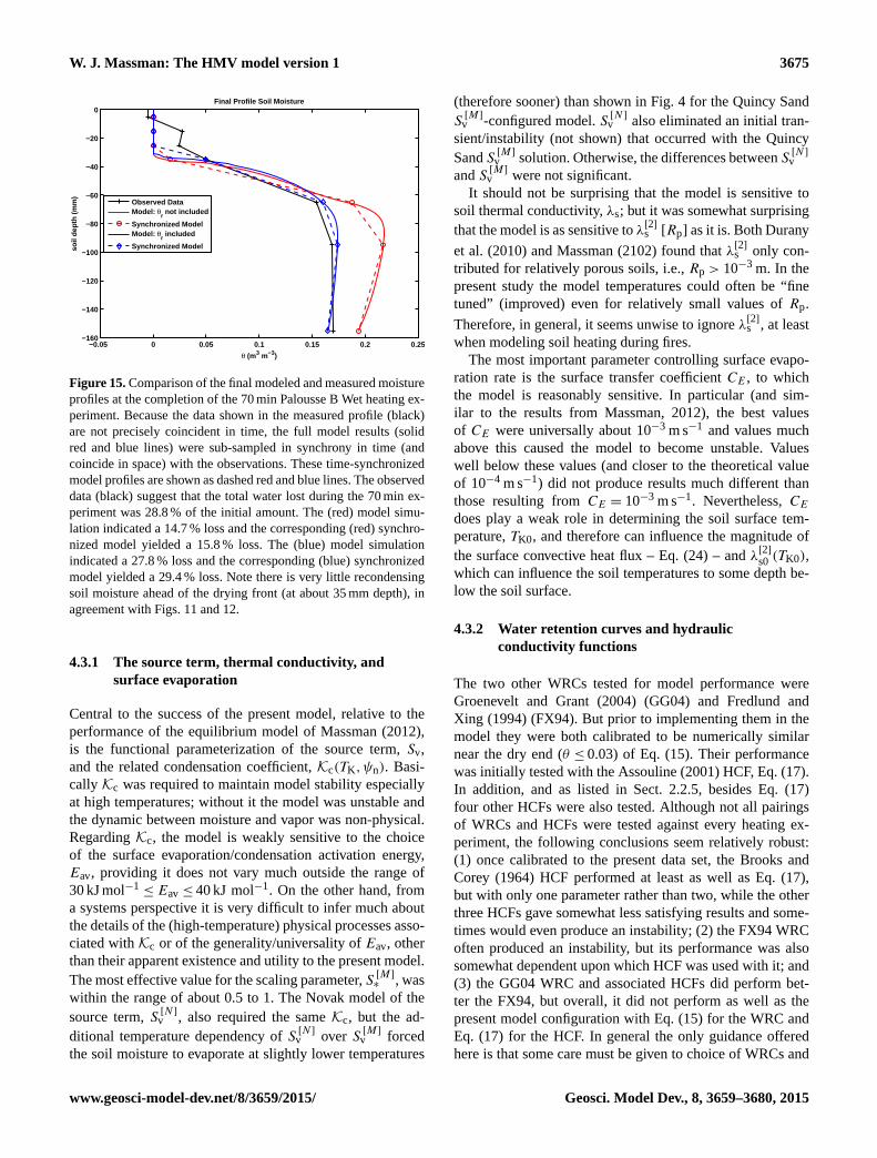
W. J. Massman: The HMV model version 1 3675
−0.05 0 0.05 0.1 0.15 0.2 0.25−160
−140
−120
−100
−80
−60
−40
−20
0
θ (m3 m−3)
soil
dep
th (
mm
)
Final Profile Soil Moisture
Observed DataModel: θ
r not included
Synchronized ModelModel: θ
r included
Synchronized Model
Figure 15. Comparison of the final modeled and measured moisture
profiles at the completion of the 70 min Palousse B Wet heating ex-
periment. Because the data shown in the measured profile (black)
are not precisely coincident in time, the full model results (solid
red and blue lines) were sub-sampled in synchrony in time (and
coincide in space) with the observations. These time-synchronized
model profiles are shown as dashed red and blue lines. The observed
data (black) suggest that the total water lost during the 70 min ex-
periment was 28.8 % of the initial amount. The (red) model simu-
lation indicated a 14.7 % loss and the corresponding (red) synchro-
nized model yielded a 15.8 % loss. The (blue) model simulation
indicated a 27.8 % loss and the corresponding (blue) synchronized
model yielded a 29.4 % loss. Note there is very little recondensing
soil moisture ahead of the drying front (at about 35 mm depth), in
agreement with Figs. 11 and 12.
4.3.1 The source term, thermal conductivity, and
surface evaporation
Central to the success of the present model, relative to the
performance of the equilibrium model of Massman (2012),
is the functional parameterization of the source term, Sv,
and the related condensation coefficient, Kc(TK,ψn). Basi-
cally Kc was required to maintain model stability especially
at high temperatures; without it the model was unstable and
the dynamic between moisture and vapor was non-physical.
Regarding Kc, the model is weakly sensitive to the choice
of the surface evaporation/condensation activation energy,
Eav, providing it does not vary much outside the range of
30 kJ mol−1≤ Eav ≤ 40 kJ mol−1. On the other hand, from
a systems perspective it is very difficult to infer much about
the details of the (high-temperature) physical processes asso-
ciated with Kc or of the generality/universality of Eav, other
than their apparent existence and utility to the present model.
The most effective value for the scaling parameter, S[M]∗ , was
within the range of about 0.5 to 1. The Novak model of the
source term, S[N ]v , also required the same Kc, but the ad-
ditional temperature dependency of S[N ]v over S
[M]v forced
the soil moisture to evaporate at slightly lower temperatures
(therefore sooner) than shown in Fig. 4 for the Quincy Sand
S[M]v -configured model. S
[N ]v also eliminated an initial tran-
sient/instability (not shown) that occurred with the Quincy
Sand S[M]v solution. Otherwise, the differences between S
[N ]v
and S[M]v were not significant.
It should not be surprising that the model is sensitive to
soil thermal conductivity, λs; but it was somewhat surprising
that the model is as sensitive to λ[2]s [Rp] as it is. Both Durany
et al. (2010) and Massman (2102) found that λ[2]s only con-
tributed for relatively porous soils, i.e., Rp > 10−3 m. In the
present study the model temperatures could often be “fine
tuned” (improved) even for relatively small values of Rp.
Therefore, in general, it seems unwise to ignore λ[2]s , at least
when modeling soil heating during fires.
The most important parameter controlling surface evapo-
ration rate is the surface transfer coefficient CE , to which
the model is reasonably sensitive. In particular (and sim-
ilar to the results from Massman, 2012), the best values
of CE were universally about 10−3 m s−1 and values much
above this caused the model to become unstable. Values
well below these values (and closer to the theoretical value
of 10−4 m s−1) did not produce results much different than
those resulting from CE = 10−3 m s−1. Nevertheless, CEdoes play a weak role in determining the soil surface tem-
perature, TK0, and therefore can influence the magnitude of
the surface convective heat flux – Eq. (24) – and λ[2]s0 (TK0),
which can influence the soil temperatures to some depth be-
low the soil surface.
4.3.2 Water retention curves and hydraulic
conductivity functions
The two other WRCs tested for model performance were
Groenevelt and Grant (2004) (GG04) and Fredlund and
Xing (1994) (FX94). But prior to implementing them in the
model they were both calibrated to be numerically similar
near the dry end (θ ≤ 0.03) of Eq. (15). Their performance
was initially tested with the Assouline (2001) HCF, Eq. (17).
In addition, and as listed in Sect. 2.2.5, besides Eq. (17)
four other HCFs were also tested. Although not all pairings
of WRCs and HCFs were tested against every heating ex-
periment, the following conclusions seem relatively robust:
(1) once calibrated to the present data set, the Brooks and
Corey (1964) HCF performed at least as well as Eq. (17),
but with only one parameter rather than two, while the other
three HCFs gave somewhat less satisfying results and some-
times would even produce an instability; (2) the FX94 WRC
often produced an instability, but its performance was also
somewhat dependent upon which HCF was used with it; and
(3) the GG04 WRC and associated HCFs did perform bet-
ter the FX94, but overall, it did not perform as well as the
present model configuration with Eq. (15) for the WRC and
Eq. (17) for the HCF. In general the only guidance offered
here is that some care must be given to choice of WRCs and
www.geosci-model-dev.net/8/3659/2015/ Geosci. Model Dev., 8, 3659–3680, 2015

3676 W. J. Massman: The HMV model version 1
HCFs because the modeling results can be quite dependent
upon the choices made.
Universal to all of HCFs tested here is Ksurfn (i.e., Vθ,surf
and its scaling parameter Dθs0; see Eqs. 20 and 21), which
as explained above was incorporated into the hydraulic diffu-
sivity,K∗n (see Eq. 6 and the related discussion). The model’s
performance was relatively insensitive to the exact value of
Dθs0 and Dθs0 ≈ 10−10 m2s−1 is as good a default value as
any other value. Furthermore, the inclusion of Vθ,surf (soil
moisture movement associated with water molecules “hop-
ping or skipping” along the soil and water surfaces) did
provide model stability when the soil moisture reached ex-
tremely low values. Including film flow,Kfilmr – Eqs. (18) and
(19), brought no discernible benefit to the model’s perfor-
mance. For less extreme conditions and for relatively coarse-
grained sand Smits et al. (2012) reached a similar conclu-
sion. Nonetheless, Kfilmr should not be discounted as unim-
portant, so further investigation into it’s utility for modeling
still seems warranted.
4.3.3 Different soils with different initial conditions
Of the remaining three heating experiments only Wet Boul-
dercreek, which had an initial soil saturation level of about
50 %, showed anything unexpected. In general, the model
was able to capture the observed soil temperatures and tem-
perature dynamics extremely well, even better than shown in
either Fig. 5 (Quincy Sand) or Fig. 14 (Palousse B). But, re-
gardless of any adjustments to any of the model parameters
the model consistently underestimated the total amount of
water evaporated (by about half), thereby also overestimat-
ing the amount of recondensing water ahead of the drying
front (see the Wet Palousse B model run without θr, Fig. 15,
as an example). On the other hand, the model was able to cap-
ture the complete drying (θ ≡ 0) of the top 30 mm of the soil
column during the Wet Bouldercreek experiment, whereas
the Quincy Sand (Fig. 6) and Palousse B (Fig. 15) experi-
ments indicated some residual soil moisture (0< θ < 0.025)
within the model’s predicted dry zone. The model’s perfor-
mance was noticeably degraded when θr was included and it
was also quite sensitive to the choice of Rp, so much so that
best model fit to temperatures required that Rp = 0, i.e., that
λ[2]s be excluded from the model. Nonetheless, the cause for
this unexpected divergence between the modeling and ob-
served soil moisture during this heating experiment is not
understood. For the present it can only be surmised that the
model’s description of evaporative dynamics of soil mois-
ture, and possibly the transport of water (both liquid and va-
por), is still incomplete.
4.3.4 The advective velocity, uvl
Unlike with the companion model (Massman, 2012), the
present model did not require reducing the magnitude of
uvl in order to maintain model stability, which again rein-
forces the impression that the present non-equilibrium model
is an improvement over equilibrium model. Nonetheless, the
present model can produce extraordinary gradients of va-
por density and vapor pressure, which begs the question of
whether such gradients could induce other types of mass
transport than that captured by the present formulation of
uvl, Eq. (9). This was tested by using a model for Darcy’s
Law type formulation based on the assumption that the ad-
vective velocity is proportional to the vapor pressure gradient
(uvl ∝−∂ev/∂z). This formulation was tested by incorporat-
ing it into the model (excluding θr). But the model became
unstable because mathematically it was strongly hyperbolic,
rather than predominantly parabolic. Further modeling de-
velopment and parameterization of uvl and vapor transport
in general are well beyond the intent of the present study.
But it is still possible to conclude that such exploration is
warranted and could help improve model performance. Fi-
nally, it should be noted that the model’s performance was
degraded when uvl was excluded from the model.
4.3.5 Different forms of Fick’s first law for the diffusive
flux
The point was made earlier that the present model was
developed assuming the mass form for the diffusive flux,
i.e., J[Mass]diff =−Dve∂ρv/∂z, but that there are other forms
that could have been used. Most notable among them
is likely to be the mass fraction form for Fick’s first
Law: J[Fraction]diff =−Dve(ρv+ ρd)∂ωv/∂z. But J
[Pressure]diff =
−Dve[Mw/(RTK)]∂ev/∂z was also previously mentioned
and was used by Campbell et al. (1995). Implementing ei-
ther of these latter two forms of Fick’s law requires amending
J[Mass]diff to include the influence of the temperature gradient
on the diffusive flux. This is most easily accomplished with
J[Pressure]diff by combining it with the ideal gas law for water
vapor, ev = ρvRTK/Mw, to yield
J[Pressure]diff =−Dve
[Mw
RTK
]∂ev
∂z=−Dve
∂ρv
∂z
−Dve
[ρv
TK
]∂T
∂z= J[Mass]diff −Dve
[ρv
TK
]∂T
∂z. (27)
A similar result is produced for J[Fraction]diff by combining it
with the ideal gas law for the dry air component of the soil
pore space air, ρd = PdRTK/Md, with the understanding that
Pd = Patmos is held constant because Patmos, the external am-
bient atmospheric pressure during the time of the experiment,
is constant and not influenced by changes in vapor pressure
within the soil column during the soil heating experiment.
Geosci. Model Dev., 8, 3659–3680, 2015 www.geosci-model-dev.net/8/3659/2015/

W. J. Massman: The HMV model version 1 3677
The final expression for J[Fraction]diff is
J[Fraction]diff =−Dve(ρv+ ρd)
∂
∂z
[ρv
ρv+ ρd
]=
−Dve
(1+ ρv/ρd)
[∂ρv
∂z−ρv
ρd
∂ρd
∂z
]=
J[Mass]diff
(1+ ρv/ρd)
−Dve
(1+ ρv/ρd)
[ρv
TK
]∂T
∂z=
J[Pressure]diff
(1+ ρv/ρd). (28)
Comparing Eqs. (27) and (28) shows that except for the
(1+ ρv/ρd) term in the denominator of J[Fraction]diff these two
expressions for Jdiff are the same. For the purposes of the sen-
sitivity test both Eqs. (27) and (28) were used with ρv as the
predicted variable (i.e., ρj+1vi and ρ
jvi are the Crank–Nicolson
finite difference variables) and T as the model variable for
the linearized coefficients (i.e., Tji ). The resulting finite dif-
ference terms were implemented into Eq. (23) and into the
finite difference equivalent of Eq. (6).
None of the model solutions resulting from either
J[Fraction]diff or J
[Pressure]diff were useful. They were all either
(a) unstable or (b), if stable, physically unrealistic. In other
words, no solution associated with either of these other two
forms of Jdiff could be found that was not largely mean-
ingless when compared to the observations. Consequently,
the only possible conclusion here is that no improvement to
the present model’s performance is possible when using ei-
ther J[Fraction]diff or J
[Pressure]diff . This in turn supports the notion
that for the physical problem considered in the present study
J[Mass]diff appears to be the preferred expression for Jdiff.
5 Summary and recommendations
This study has developed and tested a non-equilibrium (liq-
uid to vapor phase change) model for simulating heat and
moisture flow in soils during fires, but the model does as-
sume thermal equilibrium. By and large the simulations of
soil temperature and moisture are not only credible but also
often quite good. In general, all model results showed a sig-
nificant improvement over all comparable results from the
companion equilibrium model of Massman (2012).
The principal reason for the present model’s success is
the incorporation of a dynamic condensation coefficient, Kc
(parameterized as a function of temperature and soil wa-
ter potential), into the non-equilibrium evaporative source
term, Sv; both of which are modeled after the Hertz–Knudsen
equation. Physically Kc suppressed condensation in favor
of evaporation at high temperatures and soil water poten-
tials, which in turn insured model stability. Furthermore, the
non-equilibrium assumption also seemed to have improved
the parameterization (and performance) of the mass trans-
port associated with the advective velocity, uvl, relative to
the model’s of Massman (2012) and Campbell et al. (1995).
The model’s performance was further and significantly en-
hanced by the inclusion of a hydraulic conductivity function
(HCF) for liquid water transport, which was calibrated here
by “fitting” the HCF parameters to ensure that the model op-
timally reproduced the observed temperature and moisture
dynamics. This fitting procedure was necessary because no
data are (nor will be) available for the soil samples used in
the laboratory heating experiments (Campbell et al., 1995).
Another important (and novel) feature of the model is the
inclusion of a dynamic residual soil moisture θr, also param-
eterized as a function of temperature and soil water potential,
which is introduced into the model in an attempt to capture
the long evaporative tail that seems to require temperatures
well beyond 100 ◦C in order to evaporate at all. Physically
θr is intended to represent the strongly bound soil moisture,
which for the present purposes is conceptualized as a mono-
layer. Including θr was sometimes, but not always, beneficial
to model performance. So it seems worthy of further consid-
eration and possible refinement in any future studies of a sim-
ilar nature. Finally, the model is also sensitive to the thermal
infrared radiation component to the soil’s thermal conductiv-
ity (λ[2]s ; Eq. 14), which increases the thermal conductivity
within the pore space of the soil as temperature increases.
It is recommended that this term also be included and fur-
ther tested when evaluating any future models describing the
heating soils to high temperatures.
In general, the model simulates the observed soil tempera-
tures quite well. It is often slightly less precise for soil mois-
ture and the best simulations were usually a compromise
between faithfully representing the observed soil tempera-
tures or the observed soil moisture. Nonetheless, the model
does capture reasonably well many observed features of the
soil moisture dynamics, viz., it simulates an increase in soil
moisture ahead of the drying front (due to the condensation
of evaporated soil water at the front) and the hiatus in the
soil temperature rise during the strongly evaporative stage of
the soil drying. Furthermore, the model also captures the ob-
served rapid evaporation of soil moisture that occurs at rela-
tively low temperatures (50–90 ◦C), as well as some aspects
of the long evaporative tail associated with strongly bound
soil moisture. But, the model also displays a tendency to pre-
dict a greater depth of the drying front than suggested by the
observations.
Sensitivity analyses (SAs) were also performed with dif-
ferent formulations for the water retention curve, soil hy-
draulic conductivity function, one variant of the present evap-
orative source term, Sv, and different soil types with different
initial conditions. The principal conclusion from these SAs
is that some care (and testing) must be given to the selection
of the WRC and HCF, as not all of them performed equally
well. Some further investigations into the modeling benefit of
film flow as part of the HCF also seems warranted. The two
forms of Sv tested here performed about the same, and the
model’s performance (at least for soil moisture) was poor-
est compared to the experiment with the highest initial soil
www.geosci-model-dev.net/8/3659/2015/ Geosci. Model Dev., 8, 3659–3680, 2015
3678 W. J. Massman: The HMV model version 1
moisture content. No obvious explanation for this “underper-
formance” could be found, so it seems worthwhile to further
test the model for high initial saturation conditions. Finally,
it is important to test the present model’s performance and
its associated parameterizations (particularly the WRC and
HCF) against laboratory data and field data associated with
daily cycles of soil heating and moisture transport.
Acknowledgements. I would like to thank Gaylon S. Campbell
for providing the laboratory data used in this study, as well as
James W. Thomas for his insights into and discussions of the
mathematical and numerical issues I encountered during the devel-
opment of this model and Marcia L. Huber and Allan H. Harvey for
various discussions concerning the thermophysical properties of
water and aid with the published resources used in parameterizing
the self-diffusion of water vapor.
Edited by: T. Kato
References
Assouline, S.: A model for the relative hydraulic conductivity based
on the water retention curve, Water Resour. Res, 37, 265–271,
2001.
Assouline, S. and Or, D.: Conceptual and parametric representa-
tion of hydraulic properties: A review, Vadose Zone J., 12, 1–20,
doi:10.2136/vzj2013.07.0121, 2013.
Aston, A. R. and Gill, A. M.: Coupled soil moisture, heat and wa-
ter vapour transfers under simulated fire conditions, Aust. J. Soil
Res., 14, 55–66, 1976.
Bauer, T. H.: A general analytical approach toward the thermal; con-
ductivity of porous media, Int. J. Heat Mass Tran., 36, 4181–
4191, 1993.
Bear, J.: Dynamics of Fluids in Porous Media, American Elsevier
Pub. Co, New York, NY, USA, 1972.
Bridge, L., Bradean, R., Ward, M. J., and Wetton, B. R.: The anal-
ysis of a two-phase zone with condensation in a porous medium,
J. Eng. Math., 45, 247–268, 2003.
Brooks, R. H. and Corey, A. T.: Hydraulic properties of porous me-
dia, Hydrology Paper 3, Colorado State University, Fort Collins,
CO, USA, 1964.
Bücker, D., Span, R., and Wagner W.: Thermodynamic property
models for moist air and combustion gases, J. Eng. Gas Turbines
Power, 125, 374–384, 2003.
Campbell, G. S.: Soil Physics with BASIC, Elsevier, New York, NY,
USA, 1985.
Campbell, G. S. and Shiozawa, S.: Prediction of hydraulic proper-
ties of soils using particle-size distribution and bulk density data,
in: Indirect methods for estimating the hydraulic properties of
unsaturated soils, edited by: van Genuchten, M. Th., University
of California, Riverside, CA, USA, 317–328, 1992.
Campbell, G. S., Jungbauer Jr., J. D., Bidlake, W. R., and Hunger-
ford, R. D.: Predicting the effect of temperature on soil thermal
conductivity, Soil Sci., 158, 307–313, 1994.
Campbell, G. S., Jungbauer Jr., J. D., Bristow, K. L., and Hunger-
ford, R. D.: Soil temperature and water content beneath a surface
fire, Soil Sci., 159, 363–374, 1995.
Constanza-Robinson, M. S. and Brusseau, M. L.: Air-water interfa-
cial areas in unsaturated soils: evaluation of interfacial domains,
Water Resour. Res., 38, 1195, doi:10.1029/2001WR000738,
2002.
Costa, V. A. F., Mendoça M. L., and Figueiredo, A. R.: Modeling
and simulation of wetted porous thermal barriers operating under
high temperature or high heat flux, Int. J. Heat Mass Tran., 51,
3342–3354, 2008.
Cowan, I. R.: Stomatal behavior and environment, in: Advances in
Botanical Research, edited by: Preston, R. D. and Woolhouse, H.
W., Academic Press, London, UK, 117–229, 1977.
Dal Pont, S., Meftah, F., and Schrefler, B. A.: Modeling concrete un-
der severe conditions as a multiphase material, Nucl. Eng. Des.,
241, 562–572, 2011.
Danielewicz-Ferchmin, I. and Mickiewicz,A. R.: Water Density in
the Double Layer, J. Phys. Chem., 100, 17281–17286, 1996.
Dayan, A.: Self-similar temperature, pressure and moisture distribu-
tion within an intensely heated porous half space, J. Heat Transf.,
25, 1469–1476, 1982.
de Vries, D. A.: Simultaneous transfer of heat and moisture in
porous media, EOS Trans. AGU, 39, 909–916, 1958.
de Vries, D. A.: Thermal properties in soils, in: Physics of Plant En-
vironment, edited by: van Wijk, W. R., North Holland Publishing
Co., Amsterdam, the Netherlands, 201–255, 1963.
di Blasi, C.: Simultaneous heat, mass, and momentum transfer
during biomass drying, in: Developments in Thermochemical
Biomass Conversion, edited by: Bridgwater, A. V. and Boocock,
D. G. B., Springer Science+Business Media, Dordrecht, the
Netherlands, 117–131, 1997.
Durany, J., Fraga, B., and Vargas, F.: Physical modelling and nu-
merical simulation of soil heating under forest fire conditions,
in: Forest Fire Research, edited by: Viegas, D. X., ADAI/CEIF,
Coimbra, Portugal, paper no. 263 of the attached CD, 2010.
Fernández, D. P., Goodwin, A. R. H., Lemmon, E. W., Levelt Sen-
gers, J. M. H., and Williams, R. C.: A Formulation for the static
permittivity of water and steam at temperatures from 238 K to
873 K at pressures up to 1200 MPa, including derivatives and
Debye-Hückel coefficients, J. Phys. Chem. Ref. Data, 26, 1125–
1166, 1997.
Fredlund, D. G. and Xing, A: Equations for the soil-water charac-
teristic curve, Can. Geotech. J., 31, 521–532, 1994.
Gawin, D., Majorana, C. E., and Schrefler, B. A.: Numerical anal-
ysis of hydro-thermal behavior and damage of concrete at high
temperatures, Mech. Cohes.-Frict. Mat., 4, 37–74, 1999.
Grant, C. D., Groenevelt, P. H., and Robinson, N. I.: Application
of the Grant-Groenevelt soil water retention model to predict the
hydraulic conductivity, Aust. J. Soil Res., 48, 447–458, 2010.
Groenevelt, P. H. and Grant, C. D.: A new model for the soil-water
retention curve that solves the problem of residual water con-
tents, Eur. J. Soil Sci., 55, 479–485, 2004.
Gupta, H. V. and Nearing, G. S.: Debates – The future of hy-
drological sciences: A (common) path forward? Using models
and data to learn: A systems theoretic perspective on the fu-
ture of hydrological science, Water Resour. Res., 50, 5351–5359,
doi:10.1002/2013WR015096, 2014.
Harvey, A. H. and Friend, D. G.: Physical properties of water, in:
Aqueous systems at elevated temperatures and pressures: physi-
cal chemistry of water, steam and hydrothermal solutions, edited
Geosci. Model Dev., 8, 3659–3680, 2015 www.geosci-model-dev.net/8/3659/2015/

W. J. Massman: The HMV model version 1 3679
by: Palmer, D. A., Fernández-Prini, R. and Harvey, A. H., Else-
vier, Amsterdam, the Netherlands, 1–27, 2004.
Hellmann, R., Bich, E., Vogel, E., Dickinson, A. S., and Veso-
vic, V.: Calculation of the transport and relaxation proper-
ties of dilute water vapor, J. Chem. Phys., 131, 014303,
doi:10.1063/1.3158830, 2009.
Huber, M. L., Perkins, R. A., Laeseche, A., Friend, D. G., Sengers,
J. V., Assael, M. J., Metaxa, I. N., Vogel, E., Mareš, R., and
Miyagawa, K.: New international formulation for the viscosity
of H2O, J. Phys. Chem. Ref. Data, 38, 101–125, 2009.
Huber, M. L., Perkins, R. A., Friend, D. G., Sengers, J. V.,
Assael, M. J., Metaxa, I. N., Miyagawa, K., Hellmann, R.,
and Vogel E.: New international formulation for the thermal
conductivity of H2O, J. Phys. Chem. Ref. Data, 41, 033102,
doi:10.1063/1.4738955, 2012.
IAPWS (The International Association for the Properties of Water
and Steam): Revised release on the IAPWS industrial formula-
tion 1997 for the thermodynamic properties of water and steam,
available at: http://www.iapws.org (last access: 24 May 2013),
2007.
Jacobs, A. F. and Verhoef, A.: Soil evaporation from sparse natural
vegetation estimated from Sherwood numbers, J. Hydrol., 188–
189, 443–452, 1997.
Jaynes, D. B. and Rogowski, A. S.: Applicability of Fick’s law to
gas diffusion, Soil Sci. Soc. Am. J., 47, 425–430, 1983.
Jones, H. G.: Plant and Microclimate, 3rd Edition, Cambridge Uni-
versity Press, Cambridge, UK, 2014.
Jovanovic, J. D., Kneženic-Stevanovic, A. B., and Grozdanic, D. K.:
An empirical equation for temperature and pressure dependence
of liquid heat capacity, J. Taiwan Inst. Chem. Eng., 40, 105–109,
2009.
Kadoya, K., Matsunaga, N., and Nagashima, A.: Viscosity and ther-
mal conductivity of dry air in the gaseous phase, J. Phys. Chem.
Ref. Data, 14, 947–970, 1985.
Kapoor, A., Yang, R. T., and Wong, C.: Surface diffusion, Catal.
Rev., 31, 129–214, 1989.
Ki, H., Mohanty, P. S., and Mazumder, J.: A numerical method for
multiphase incompressible thermal flows with solid-liquid and
liquid-vapor phase transformations, Numer. Heat Tr. B Fund., 48,
125–145, 2005.
Kon, M., Kobayashi, K. and Watanabe, M.: Method of
determining kinetic boundary conditions in net evapora-
tion/condensation, Phys. Fluids (1994–present), 26, 072003,
doi:10.1063/1.4890523, 2014.
Kozlowski, T.: Modulated Differential Scanning Calorimetry
(MDSC) studies on low-temperature freezing of water adsorbed
on clays, apparent specific heat of soil water and specific heat of
dry soil, Cold Reg. Sci. Technol., 78, 89–96, 2012.
Leij, F. J., Schaap, M. G., and Arya, L. M.: Indirect Methods, in:
Methods of Soil Analysis Part 4: Physical Methods, co-edited
by: Dane, J. H. and Topp, G. C., Soil Sci. Society of America
Inc., Madison, WI, USA, 1009–1045, 2002.
Liu, B. C., Liu, W., and Peng, S. W.: Study of heat and moisture
transfer in soil with a dry surface layer, Int. J. Heat Mass Tran.,
48, 4579–4589, 2005.
Marrero, T. R. and Mason, E. A.: Gaseous diffusion coefficients, J.
Phys. Chem. Ref. Data, 1, 3–118, 1972.
Massman, W. J.: Modeling soil heating and moisture transport un-
der extreme conditions: Forest fires and slash pile burns, Water
Resour. Res., 48, W10548, doi:10.1029/2011WR011710, 2012.
Medved, I. and Cerný, R.: Surface diffusion in porous media: A
critical review, Micropor. Mesopor. Mat., 142, 405–422, 2011.
Miles, R. E. H., Reid, J. P., and Rüpinen, I.: Comparison of ap-
proaches for measuring the mass accommodation coefficient for
the condensation of water and sensitivities to uncertainties in
thermophysical properties, J. Phys. Chem. A, 116, 10810–10825,
2012.
Milly, P. C. D.: Moisture and heat-transport in hysteretic, inhomo-
geneous porous media: A matric head-based formulation and a
numerical model, Water Resour. Res., 18, 489–498, 1982.
Moldrup, P. T., Olesen, D. E., Roslton, D. E., and Yamaguchi, T.:
Modeling diffusion and reactions in soils: VII. Predicting gas
and ion diffusivity in undisturbed and sieved soils, Soil Sci., 162,
632–640, 1997.
Novak, M. D.: Dynamics of the near-surface evaporation zone and
corresponding effects on the surface energy balance of a drying
soil, Agr. Forest Meteorol., 150, 1358–1365, 2010.
Novak, M. D.: Comment on “Evaporation from soils under thermal
boundary conditions: Experimental and modeling investigation
to compare equilibrium- and nonequilibrium-based approaches”
by Kathleen M. Smits, Abdullah Cihan, Toshihiro Sakaki, and
Tissa H. Illangasekare, Water Resources Research, 48, W05549,
doi:10.1029/2011WR011393, 2012.
Ouedraogo, F., Cherblanc, F., Naon, B., and Bénet, J.-C.: Water
transfer in soil at low water content. Is the local equilibrium as-
sumption still appropriate?, J. Hydrology 492, 117–127, 2013.
Pakala, V. K. C. and Plumb, O. A.: High intensity drying in
porous materials, J. Thermal Sci. Eng. Appls., 4, 021010,
doi:10.1115/1.4006275, 2012.
Philip, J. R. and de Vries, D. A.: Moisture movement in porous ma-
terials under temperature gradients, EOS Trans. AGU, 38, 222–
232, 1957.
Sato, H.: An equation of state for the thermodynamic properties
of water in the liquid phase including the metastable state, in:
Properties of Water and Steam Proceedings of the 11th Inter-
national Conference, 4–8 September 1989, Prague, Czechoslo-
vakia, edited by: Píchal, M. and Šifner, O., Hemisphere Publish-
ing Company, New York, NY, USA, 48–55, 1990
Shiozawa, S. and Campbell, G. S.: On the calculation of mean par-
ticle diameter and standard deviation from sand, silt, and clay
fractions, Soil Sci., 152, 427–431, 1991.
Skopp, J.: Oxygen uptake and transport in soils: analysis of the
air-water interfacial area, Soil Sci. Soc. Am. J., 49, 1327–1331,
1985.
Smits, K. M., Cihan, A., Sakaki, T., and Illangasekare, T. H.:
Evaporation from soils under thermal boundary conditions: Ex-
perimental and modeling investigation to compare equilibrium-
and nonequilibrium-based approaches, Water Resour. Res., 47,
W05540, doi:10.1029/2010WR009533, 2011.
Smits, K. M., Ngo, V. V., Cihan, A., Sakaki, T., and Illangasekare T.
H.: An evaluation of models of bare soil evaporation formulated
with different land surface boundary conditions and assumptions,
Water Resour. Res., 48, W12526, doi:10.1029/2012WR012113,
2012.
Solsvik, J. and Jakobsen, H. A.: A Survey of multicomponent mass
diffusion flux closures for porous pellets: Mass and molar forms,
www.geosci-model-dev.net/8/3659/2015/ Geosci. Model Dev., 8, 3659–3680, 2015

3680 W. J. Massman: The HMV model version 1
Transport Porous Med., 93, 99–126, doi:10.1007/s11242-012-
9946-7, 2012.
Somayajulu, G. R.: New equations for enthalpy of vaporization
from the triple point to the critical point, Int. J. Thermophysics,
9, 567–575, 1988.
Thomas, J. C.: Numerical partial differential equations: finite differ-
ence methods, Springer, New York, NY, USA, 1985.
Tsilingiris, P. T.: Thermophysical transport properties of humid air
at temperature range between 0 and 100 ◦C, Energy Conservation
and Management, 49, 1098–1110, 2008.
Tsuruta, T. and Nagayama, G.: Molecular dynamics studies on the
condensation coefficient of water, J. Phys. Chem. B, 108, 1736–
1743, 2004.
Udell, K. S.: Heat transfer in porous media heated from above with
evaporation, condensation, and capillary effects, J. Heat Transf.,
105, 485–492, 1983.
Van Genuchten, M. Th. and Nielsen, D. R.: On describing and pre-
dicting the hydraulic properties of unsaturated soils, Ann. Geo-
phys., 3, 615–628, 1985,
http://www.ann-geophys.net/3/615/1985/.
Vargaftik, N. B., Volkov, B. N., and Voljak, L. D.: International ta-
bles of the surface tension of water, J. Phys. Chem. Ref. Data,
12, 817–820, 1983.
Wagner, W. and Pruess, A.: The IAPWS formulation 1995 for the
thermodynamic properties of ordinary water substance for gen-
eral and scientific use, J. Phys. Chem. Ref. Data, 31, 387–535,
2002.
Whitaker, S.: Simultaneous heat, mass and momentum transfer in
porous media: a theory of drying, Adv. Heat Trans., 13, 119–203,
1977.
Whitaker, S. and Chou, W. T.-H.: Drying granular porous media –
Theory and experiment, Drying Technol., 1, 3–33, 1983–1984.
Yaws, C.: Handbook of Transport Property Data, Gulf Publishing
Company, Houston, TX, USA, 1995.
Yoshida, K., Matubayasi, N., and Nakahara, M.: Self-diffusion of
supercritical water in extremely low-density region, J. Chem.
Phys., 125, 074307, doi:10.1063/1.2333511, 2006.
Yoshida, K., Matubayasi, N., and Nakahara, M.: Erratum: “Self-
diffusion of supercritical water in extremely low-density region”,
J. Chem. Phys., 126, 089901, doi:10.1063/1.2372501, 2007.
Zhang, Z. F.: Soil water retention and relative permeability for con-
ditions from oven-dry to full saturation, Vadose Zone J., 10,
1299–1308, doi:10.2136/vzj2011.0019, 2011.
Geosci. Model Dev., 8, 3659–3680, 2015 www.geosci-model-dev.net/8/3659/2015/