a non-gaussian family of state-space models with exact
TRANSCRIPT
A non-Gaussian family of state-space modelswith exact marginal likelihood
Dani Gamermana Thiago Rezende dos Santosb Glaura C. Francob∗
aDepartment of Statistical Methods, Universidade Federal do Rio de Janeiro, RJ, Brazil.bDepartment of Statistics, Universidade Federal de Minas Gerais, MG, Brazil.
Abstract
The Gaussian assumption generally employed in many state space models isusually not satisfied for real time series. Thus, in this work a broad familyofnon-Gaussian models is defined by integrating and expanding previous work inthe literature. The expansion is obtained at two levels: at the observationallevelit allows for many distributions not previously considered and at the latentstatelevel it involves an expanded specification for the system evolution. The class re-tains analytical availability of the marginal likelihood function, uncommon outsideGaussianity. This expansion considerably increases the applicability of themodelsand solves many previously existing problems such as long-term prediction, miss-ing values and irregular temporal spacing. Inference about the state componentscan be performed due to the introduction of a new and exact smoothing proce-dure, in addition to filtered distributions. Inference for the hyperparameters is pre-sented from the classical and Bayesian perspectives. Performanceof the model canbe assessed through diagnostic tools and predictive and fit measures.The resultsseem to indicate competitive results of the models when compared to other non-Gaussian state-space models available. The methodology is applied to Gaussianand non-Gaussian dynamic linear models with time-varying means and variancesand provides a computationally simple solution to inference in these models. Themethodology is illustrated in a number of examples, including time series withunknown data support. The paper is concluded with directions for further work.
Keywords: classical inference; Bayesian; forecasting; non-linear system evo-lution; smoothing.
1 Introduction
Several models are built in the literature based on the normality, homoscedasticity andindependence assumptions of the errors. However, in many situations, these assump-tions are not satisfied. Error independence is rarely attained in the time series context,while the normality assumption is often discarded in a wide variety of situations.
∗Correspondence author: Glaura C. Franco. Address: Universidade Federal de Minas Gerais, Belo Hori-zonte, MG, 31270-901, Brazil. E-mail:[email protected]
1

Many state space models (SSM) use results based on normality(Harvey, 1989;West & Harrison , 1997, see) largely due to their analytical tractability. This nice andcomputationally convenient feature is lost once the normality assumption is removed.The goal of this paper is to present possibilities for analyzing time series under theSSM framework beyond Gaussianity while still retaining tractability.
The origin of this work can be traced back to Nelder & Wedderburn (1972), whoproposed thegeneralized linear models(GLM). The basic idea of these models consistsin opening the range of options for the response-variable distribution, by allowing it tobelong to the exponential family of distributions. According to Nelder & Wedderburn(1972), a link function is used to relate the mean function ofthe data to the linearpredictor. The paper of Nelder & Wedderburn (1972) was concerned with independentdata, while in the time series context, the observations generally present a correlationstructure.
In this direction, a more general structure, calledDynamic Generalized LinearModels(DGLM), proposed by West, Harrison & Migon (1985), attracted a great dealof interest due to the applicability of GLM in time series. Papers in this context in-clude Grunwald, Raftery & Guttorp (1993), Fahrmeir & Kaufmann (1987), Lindsey& Lambert (1995), Gamerman (1991, 1998), Chiogna & Gaetan (2002), Shephard& Pitt (1997) and Godolphin & Triantafyllopoulos (2006). The books by Durbin &Koopman (2001) and Fahrmeir & Tutz (2001) also present and discuss these modelsin addition to providing alternatives for analyzing non-Gaussian time series. The prob-lem with this class of models is that the analytical form is easily lost, even using simplemodel components. Thus, the predictive distribution, thatis essential for the inferenceprocess, can only be obtained approximately.
Many researchers have worked in the last decades in auxiliary procedures in orderto make inference for non-Gaussian state space models underthe Bayesian approach.Gamerman (1998) proposed a GLM based MCMC algorithm for inference, Fruhwirth-Schnatter & Wagner (2006) used auxiliary mixture sampling and Pitt & Walker (2005)utilized auxiliary variables for constructing stationarytime series. Andrieu & Doucet(2002) and Carvalho et al. ( 2010) are just a sample of a large community devotedto inference via sequential Monte Carlo or particle filtering in the state space modelscontext. However, it is important to emphasize that these methods are approximatedand the computing time can be large.
The objective of this paper is to present a family of models that allows for exact,analytical computation of the marginal likelihood and thusthe predictive distribution.This family is obtained by generalizations of results from Smith & Miller (1986).They considered an exponential observational model and an exact evolution equationthat enables the analytical integration of the state and theattainment of the 1-step-aheadpredictive distributions. Harvey & Fernandes (1989) and Shephard (1994) showed thatthe same tractability was obtained with Poisson and normal scale observational models,respectively. The family introduced in this paper unifies these and several other modelsthat were treated separately. Additionally, an expanded evolution equation is proposed,thus allowing for exact expression for long-term prediction. It will also be seen thatthese exact computations are very easy to code.
Thus, the main contributions of this paper are to consider and to characterize thisfamily of models, by presenting special cases of observational time series that belong
2

to this family. In addition, a smoothing procedure, similarto the forward filteringbackward sampling (FFBS) algorithm used in Gaussian SSM, isalso introduced. Gen-eral expressions fork-step-ahead predictions are provided and treatment of timeseriescontaining missing data and/or unequally spaced observation times is considered. Theideas of these models are also applied to Gaussian and non-Gaussian dynamic linearmodels and are shown to provide a computationally simple solution to the problem ofestimation when both means and variances are subject to temporal variation.
The paper is organized as follows. The models are presented in Section 2, wherethe main theoretical results for filtered or on-line inference for the latent variables andprediction of future observations are provided. Section 3 introduces the smoothingprocedure, vital for inference on the latent variables based on the complete time series.Section 4 presents the inferential procedure for the model hyperparameter from classi-cal and Bayesian perspectives. Point and interval estimation procedures are describedin addition to model checking procedures. Section 5 revisits dynamic linear models andshows how the methods of this paper can be adapted to cope withtime-varying obser-vational means and variances. Section 6 presents illustrative analysis of real data seriesin a number of areas of application. Finally, Section 7 presents the main conclusionsand final remarks.
2 Model definition and properties
In this section, the models are introduced. They are a generalization and integration ofthe non-Gaussian dynamic models of Smith & Miller (1986) andHarvey & Fernandes(1989). The main advantage of these models compared to the DGLM is that exactinference can be performed. Due to the form of the model equations, some commoncomponents, such as seasonality and influence of other predictor series, are inserted asfixed effects.
A time series{yt} is in this class of models if it satisfies the following assumptions:
A0 its probability (density) function can be written in the form:
p(yt|µt, µt−1, . . . , µ1,Y t−1,ϕ) = p(yt|µt,Y t−1,ϕ)
= a(yt,ϕ)µb(yt,ϕ)t exp (−µtc(yt,ϕ)) ,(1)
for yt ∈ S(ϕ) ⊂ ℜ andp(yt|µt,ϕ) = 0, otherwise. Functionsa(·), b(·), c(·)andS(·) are such thatp(yt|µt,ϕ) ≥ 0 and thereforeµt > 0, for all t > 0. It isalso assumed thatϕ varies in thep-dimensional parameter spaceΦ.
A1 If xt is a covariate vector, the link functiong relates the predictor to the parameterµt through the relationµt = λtg(xt,β), whereβ are the regression coefficients(one of the components ofϕ) andλt is the latent state variable related to the de-scription of the dynamic level. If the predictor is linear, theng(xt,β) = g(x
′
tβ).
A2 The dynamic levelλt evolves according to the system equationλt+1 =w−1λtςt+1 whereςt+1|Y t,ϕ ∼ Beta (wat, (1− w)at), that is,
wλt+1
λt| λt,Y t,ϕ ∼ Beta (wat, (1− w)at) ,
3

whereat are known constants to be specified later in the text,0 < w ≤ 1,Y t = {Y0, y1, . . . , yt}, for t = 1, 2, ... andY0 represents previously availableinformation.
A3 The dynamic levelλt is initialized with prior distributionλ0|Y0 ∼ Gamma(a0, b0).
The data-dependent evolutionA2 is not usually encountered in most SSM but doesnot invalidate model specification. Appendix A details the calculations that prove thatthe state-space model above is well-defined even with this evolution.
There is a wide range of distributions that belong to this class of models. It includesmany commonly known discrete and continuous distributionssuch as Poisson, Gammaand Normal (with static mean) but also includes many other distributions that are notso common.
Table 1 provides the form of functionsa, b, c andS for some distributions in thisfamily. The more common cases such as Poisson and Exponential were previouslysingled out in the literature. Several other cases of this family are introduced hereand they include continuous and discrete distributions. Some of them are well knownsuch as Normal and Pareto but the family includes also the Borel-Tanner (Haight &Breuer , 1960) and the Rayleigh distributions, for example.The picture that emerges isa collection that is capable of representing a variety of features that are present in timeseries applications and thus are of practical importance.
Table 1: Special cases of the non-Gaussian SSM.Models ϕ a(yt,ϕ) b(yt,ϕ) c(yt,ϕ) S(ϕ)
Poisson (w, β)′
(yt!)−1 yt 1 {0, 1, . . .}
Borel-Tanner (w, ρ, β) ρ(yt−ρ)!
yyt−ρ−1t yt − ρ yt {ρ, ρ+ 1, . . .}
Gamma (w,χ, β) yχ−1t /Γ(χ) χ yt (0,∞)
Weibull (w, ν, β) ν(yt)ν−1 1 (yt)
ν (0,∞)Pareto (w, ρ, β) y−1
t 1 ln yt − ln ρ (ρ,∞)Normal (w, θ) (2π)−1/2 1/2 (yt − θ)2/2 (−∞,∞)Laplace (w, θ) 1√
21
√2 |yt − θ| (−∞,∞)
Inverse Gaussian (w, θ) 1√2πy3
t
1/2 (yt−θ)2
2ytθ2(0,∞)
Rayleigh (w, θ) yt 1 12(yt − θ)2 (0,∞)
Power Exponential (GED)(w, ν, κ, θ) ν
κ2ν+1ν Γ(1/ν)
1/ν (yt−θ)ν
2κν (−∞,∞)
Generalized Gamma (w, ν, χ) νyνχ−1t /Γ(χ) χ yν
t (0,∞)
The usual specification for the link functiong is the logarithmic function given thepositive nature ofµt, but other link functions dictated by the application may also beused. It is interesting to note that the evolution equation can be rewritten asln(λt) =ln(λt−1) + ς∗t , whereς∗t = ln(ςt/w) ∈ ℜ, similar to the random walk evolution of thenon-Gaussian local level model. The main difference with respect to other commonnon-Gaussian SSM is the use of the scaled log-Beta disturbances instead of normaldisturbances. This change proves vital for obtaining exactresults.
The parameterw varies between 0 and 1 and also belongs toϕ. As it will be seenin what follows,w is responsible for increasing the variance over time. Thus,it plays
4
a similar role to that of discount factors, used in the Bayesian approach to state spacemodels.
The family inA0 is quite general and functionsa, b andc must satisfy constraintsto ensure a proper distribution. Many properties can also bederived as, for example,E[b(yt,ϕ)] = µtE[c(yt,ϕ)]. However, these derivations are not required in the sequeland are not pursued here. Ifb(yt,ϕ) = b(y) or c(yt,ϕ) = c(y) andS(ϕ) does notdepend onϕ, the observational model inA0 becomes a special case of the exponentialfamily of distributions.
Theorem 1 below provides basic results of these models for sequential or on-lineinference for the levelλt (filtering results) and the predictive distribution.
Theorem 1. If the model is defined inA0-A3, the following results can be obtainedfor t=1, 2, ...
1. the prior distributionλt|Y t−1,ϕ follows a Gamma(at|t−1, bt|t−1) distributionsuch that
at|t−1 = wat−1, (2)
bt|t−1 = wbt−1. (3)
2. The on-line or updated distribution ofλt|Y t,ϕ is Gamma (at,bt), where
at = at|t−1 + b(yt,ϕ), (4)
bt = bt|t−1 + c(yt,ϕ). (5)
3. The one step ahead predictive density function is given by
p(yt|Y t−1,ϕ) =Γ(b(yt,ϕ) + at|t−1)a(yt,ϕ)(bt|t−1)
at|t−1
Γ(at|t−1)[c(yt,ϕ) + bt|t−1]b(yt,ϕ)+at|t−1
, yt ∈ S(ϕ),
(6)∀t ∈ N andΓ(·) is the gamma function.
The proof of Theorem 1 is in Appendix B.The corresponding distribution ofµt = λtg(xt,β) is easily obtained from Items 1
and 2 of Theorem 1, using the scale property of the Gamma distribution. For example,µt|Yt ∼ Gamma
[at, bt(g(xt,β))
−1].
Note from (2)-(3) thatE(λt|Y t−1) = E(λt−1|Y t−1) andV ar(λt|Y t−1,ϕ) =w−1V ar(λt−1| Y t−1,ϕ). The passage of time fromt− 1 to t implies that means arepreserved but only100w% of the information (in terms of precision) is retained. Thisisexactly the role of the discount factors used in West & Harrison (1997). Theorem 1 en-ables exact inference about the state parameters whenϕ is known. This is a distinctivefeature of the modelsA0-A3 and it is rarely seen outside linear normal SSM.
The model can be trivially extended for time-varyingw. One would simply replacew by wt in A2 and the only changes implied are replacement ofw by wt in item 1 of
5

Theorem 1. This issue allows extra flexibility that will prove important for handlingirregularities such as missing points or temporally unequal-spaced observations.
Longer term predictions can be obtained by applying the evolution repeatedly overtime. The predictive distributions are obtained by
f(yt+h|Y t,ϕ) =
∫f(yt+1:t+h|Y t,ϕ) dyt+1:t+h−1
=
∫ h∏
j=1
f(yt+j |Y t+j−1,ϕ) dyt+1:t+h−1 (7)
where the notation of Apendix A is used for indexing vectors.This integration cannot be performed analytically. Nevertheless, (7) providesthe way to sample from(yt+h|Y t,ϕ). This is described in the algorithm below:
1. setj = 1;
2. drawyvt+j from f(yt+j |Y t+j−1,ϕ) and setY t+j = {Y t+j−1, yvt+j};
3. setj → j + 1 and return to 1, ifj ≤ h; otherwise, stop.
In many cases, drawsyvt+j from f(yt+j |Y t+j−1,ϕ) are easier to obtain with the in-termediate step of a drawλv
t+j from f(λt+j |Y t+j−1,ϕ) followed by drawingyvt+j
from f(yt+j |λvt+j ,Y t+j−1,ϕ). Note also thatyvt+1:t+h = (yvt+1, ..., y
vt+h) are a joint
sample from the predictive trajectoryf(yt+1:t+h|Y t,ϕ).The distribution in (7) describes the uncertainty associated with the time series fore-
casts. Summary measures, like mean, median and percentilescan be easily extractedfrom them. These results are based on knowledge ofϕ. The procedures required whenϕ is unknown are described in Section 4.
Unfortunately, analytic expressions for these predictivedistributions are not avail-able. The multiplicative nature of the evolution may be usedas a basis to obtain analyticapproximations. It suggests that theh-steps ahead evolution could be approximated by
λt+h|Y t,ϕ ∼ Gamma(at+h|t, bt+h|t) (8)
whereat+h|t = what andbt+h|t = whbt. This would lead to the predictive densityfunction of the observationsh steps ahead
p(yt+h|Y t,ϕ) =Γ(b(yt+h,ϕ) + at+h|t)a(yt+h,ϕ)(bt+h|t)
at+h|t
Γ(at+h|t)[c(yt+h,ϕ) + bt+h|t]b(yt+h,ϕ)+at+h|t
, yt+h ∈ S(ϕ).
(9)Appendix B shows that predictive distributions (8) and (9) are obtained ifA2 weregeneralised to
wλt+h+1
λt+h| λt+h,Y t, ,ϕ ∼ Beta
(wh+1at, (1− w)what
), for h = 0, 1, 2, ...,
(10)Simulations not reported here show that assumption (10) andhence density (9) providereasonable approximations for single digit horizons and could be used as an alternative.
6

The above results could be used in conjunction with a time-varyingw for handlingirregularly spaced series and missing observations. If a collection of r observationsare missing after times thenw could be replaced bywr for the evolution at times. Similarly, if observations are collected at timest1, t2, ... then this data irregularitycould be reflected by respective replacements ofw bywti−ti−1 , for all i.
3 Smoothing
The main interest in many situations is to estimate the levelcomponentλ = (λ1, . . . , λn)′
based on all available informationY n instead of the sequence of marginal on-line dis-tributionsλt|Y t, ∀t. Smoothing techniques should be used in these cases. Harvey&Fernandes (1989) present an estimate of the level componentin an application to a realseries, obtained by using an approximated smoothing algorithm of fixed interval (Har-vey, 1989). They acknowledge the approximating nature of their scheme by naming itaquasi-smoothingprocedure.
In the normal linear context, the joint distribution of all state parameters given allavailable information is multivariate normal and its expression is given in Migon etal. (2005). The precision or inverse covariance matrix is intridiagonal block form,as a reflection of the Markovian structure of the model. This opens up the possibilityfor devising better schemes based on the sparcity of this matrix. This is speciallyrelevant when the time series lengthn is large. One such scheme is the FFBS algorithmproposed by Fruhwirth-Schnatter (1994) and Carter & Kohn (1994). This algorithmshows how the multivariate normal joint distribution of thestates can be broken downinto smaller but still normal components.
The FFBS decomposition is always possible in SSM but the linear normal SSMis the only known situation where it leads to a tractable solution. Theorem 2 belowprovides a non-Gaussian version of FFBS for the models of this paper, showing thatthey also lead to a tractable solution.
Theorem 2.The joint distribution of(λ|Y n,ϕ) has density
p(λ|ϕ,Y n) = p(λn|ϕ,Y n)
n−1∏
t=1
p(λt|λt+1,ϕ,Y t)p(ϕ|Y n),
where the distribution of(λt|λt+1,ϕ,Y t), is given by
λt − wλt+1|λt+1,ϕ,Y t ∼ Gamma((1− w)at, bt) , ∀t ≥ 0. (11)
Proof of Theorem 2 can be found in Appendix B.Based on Theorem 2, an exact sample of the joint distributionof (λ|ϕ,Y n) can be
obtained following the algorithm below:
1. sett = n and samplep(λn|ϕ,Y n), using Theorem 1 witht = n;
2. sett = t− 1 and samplep(λt|λt+1,ϕ,Y t), using (11);
7

3. if t > 1, go back to step 2; otherwise, the sample of(λ1, . . . , λn|ϕ,Y n) iscomplete.
The result in (11) allows the implementation of step 2 of the algorithm above andthus enables an exact sample from the smoothed distributionof the states once thehyperparameter is known. This result will prove to be crucial for inference about thestates even when the hyperparameter is not known.
4 Inference for hyperparameters
The model parameters were divided into the latent states{λt} and fixed parametersϕ, usually called hyperparameters. Theon-line and smoothed inference for the stateparameters were presented in Sections 2 and 3, respectively. Knowledge of the hyper-parameter was assumed in both cases. In this section, inference for the hyperparametersand the latent states is discussed.
4.1 Classical Inference
One way of making classical inference about the parameter vector ϕ is through themarginal likelihood function, whose form is given by
L(ϕ;Y n) =n∏
t=1p(yt|Y t−1,ϕ) =
n∏t=1
Γ(b(yt,ϕ)+at|t−1)a(yt,ϕ)(bt|t−1)at|t−1
Γ(at|t−1)[c(yt,ϕ)+bt|t−1]b(yt,ϕ)+at|t−1
, (12)
whereyt ∈ S(ϕ) andϕ is composed byw, β and by parameters of the specific model.Maximization of the marginal likelihood function (12) is typically performed numeri-cally.
The Gamma prior distribution used as the initial distribution forµt tends to becomenon-informative whena0, b0 → 0, and is improper whena0 = b0 = 0. Note that ifa0, b0 → 0, the on-line distribution of(λ1|Y 1) can be improper, so that the predictivedensity function will not be defined. Thus, from now on it willbe assumed thata0 > 0andb0 > 0. If a0 = b0 = 0, the indext in the product above can be initialized at instantt = τ instead oft = 1, whereτ is the smallest value oft for which the distribution of[λt|Y t] is proper.
Under some regularity conditions, the asymptotic properties of the maximum like-lihood estimator (MLE) (Harvey, 1989, page 128) lead to
I1/2n (ϕ)(ϕ−ϕ)D→N[0, Ip], (13)
whereϕ is the MLE ofϕ, In(ϕ) is the Fisher information matrix andIp is the iden-tity matrix of dimensionp. The conditions are satisfied for the non-Gaussian SSM,subjected to:
1. ϕ is an interior point of the parametric space. This happens ifw < 1 and allother components ofϕ defined in the positive line are not equal to zero.
8

2. the derivatives, at an arbitrary instantt, for t = 1, . . . , n, exist and can be com-puted by derivation of the predictive density function in (6) with respect toϕand its continuity is the result of the continuity ofat|t−1 andbt|t−1. When oneof the model parameters depends on the support, the derivatives of the respectiveparameter may not exist.
3. two different pointsϕ1 andϕ2 will produce different models and, as a result,different values for the likelihood function.
The asymptotic confidence interval forϕ is built based on a numerical approxi-mation for In(ϕ), usingIn(ϕ) ∼= −H(ϕ), where−H(ϕ) is the matrix of secondderivatives of the log-likelihood function with respect tothe parameters.
Let ϕi, i = 1, . . . , p, be any component ofϕ. Then, an asymptotic confidenceinterval of100(1− κ)% for ϕi is given by
ϕi ± zκ/2
√V ar(ϕi),
wherezκ/2 is theκ/2 percentile of the standard normal distribution andV ar(ϕi) isobtained from the diagonal elements of the Fisher information matrix.
The observed information matrix is asymptotically equivalent to the expected in-formation matrix (Migon & Gamerman, 1999). This result seems to be corroboratedfor SSM through simulation in Cavanaugh & Shumway (1996). Approximation of theexpected information matrix by the observed information matrix is relatively commonand suggested in many texts like Cavanaugh & Shumway (1996) and Sallas & Harville(1988), mainly for large samples.
Asymptotic confidence intervals can present border problems, that is, the inter-val limits can overtake the borders of the parametric space.In these cases, the Deltamethod (Casella & Berger, 2002) could be used to solve the problem by appropriatelytransforming the components ofϕ to the real line.
Inference for the latent variables can be made in a number of forms. The simplestis to replaceϕ by its MLE estimator in the calculations of Sections 2 and 3. The mainadvantage of this plug-in procedure is its simplicity. It also provides adequate meanestimates but has the drawback of underestimating the uncertainty associated with theestimation ofϕ. Alternatives taking into account this uncertainty may be available viabootstrap procedures. Similar comments are valid for the predictive distributions.
4.2 Bayesian Inference
Bayesian inference forϕ can be performed using MCMC algorithms (Gamerman &Lopes, 2006), since the posterior distribution of the hyperparameter is not analyticallytractable. The marginal posterior distribution of parameter vectorϕ is given by
π(ϕ|Y n) ∝ L(ϕ;Y n)π(ϕ), (14)
whereL(ϕ;Y n) is the likelihood function defined in (12) andπ(ϕ) is the prior distri-bution ofϕ. In this work, proper uniform priors are used forϕ.
9

Credibility intervals forϕi, i = 1, ..., p are built as follows. Given a value0 < κ <1, the interval[c1, c2] satisfying
c2∫
c1
π(ϕi | Y n) dϕi = 1− κ
is a credibility interval forϕi with level100(1− κ)%.Inference for the latent variables can be made with the output from the MCMC
algorithm. Once a sampleϕ(1), ...,ϕ(M) is available, posterior samplesλ(1), ..., λ(M)
from the latent variables are obtained as follows:
1. setj = 1;
2. sample the hyperparameterϕ(j) from the MCMC algorithm;
3. sample the setλ(j) of latent variables fromp(λ|ϕ(j),Y n) using Theorem 2;
4. setj → j + 1 and return to 1, ifj ≤ M ; otherwise, stop.
Again, similar comments are valid for the predictive distributions. Note that
p(yt+h|Y t) =
∫p(yt+h|Y t,ϕ) π(ϕ|Y n) dϕ. (15)
Thus,h-step-ahead predictive distributions can be approximatedby
1
M
M∑
j=1
p(yt+h|Y t,ϕ(j))
from which summaries such as means, variances and credibility intervals can be ob-tained. Sincep(yt+h|Y t,ϕ) is not available analytically, a drawy(s)t+h fromp(yt+h|Y t)
can be obtained from (15) by samplingϕ(s) from π(ϕ|Y n) and then samplingy(s)t+h
from p(yt+h|Y t,ϕ(s)).
4.3 Model adequacy
Model adequacy is an important topic of the modeling process. Some of the diagnosticmethods suggested in the literature are described below.
Harvey & Fernandes (1989) suggest diagnostic methods basedon the (standard-ized) Pearson residuals, given by
νpt =yt − E(yt|Y t−1,ϕ)
DP (yt|Y t−1,ϕ), (16)
whereDP (yt|Y t−1,ϕ) is the standard deviation of the distribution ofyt|Y t−1,ϕ.The diagnostic methods referred by them are:
10

1. examination of residual graphs versus time and versus an estimate of the levelcomponent.
2. check whether the sample variance of the standardized residuals is close to 1. Avalue greater (smaller) than 1 indicates overdispersion (underdispersion) of themodel.
Another alternative is to use the deviance residuals (McCullagh & Nelder, 1989),which are defined by:
νdt =
{2 ln
[p(yt|yt,ϕ)
p(yt|γt,ϕ)
]}1/2
, (17)
whereγt = E(yt|Y t−1,ϕ).For example, in the Poisson model, the deviance residual is
νdt =
{2 ln
[yyt
t exp(−yt)/yt!
γtyt exp(−γt)/yt!
]}1/2
= {2 [yt ln(yt/γt)− (yt − γt)]}1/2
,
whereγt = at+1|t/bt+1|t. Diagnostic plots, like residuals versus order and fitted val-ues, may also be used.
Sometimes, it is possible to have more than one model for modeling the data, but itis required to choose one of them. Therefore, some fit criteria are needed for decidingwhich model to choose.
According to Harvey (1989, page 80), the AIC and BIC criterion are the most usedin practice. They are given by
AIC = −2log L(ϕ;Y n)
n+
2p
nandBIC = −2
log L(ϕ;Y n)
n+
p ln(n)
n,
wherep is the number of parameters andn the number of observations.The DIC criterion (Deviance Information Criterion) (Spiegelhalteret al. , 2002)
can also be used for comparing models under the Bayesian approach. It is also basedon the log likelihood with a penalization term to account formodel complexity and canbe approximated with an MCMC sample fromp(ϕ|Y n).
5 Dynamic linear models revisited
The results of this paper are also useful to a closely relatedand very frequently usedtime series model. One of the most important classes of state-space models is formedby the dynamic linear models proposed by West & Harrison (1997) for Gaussian ob-servations with time varying means and variances. Their model is easily extended byconsideration of non-Gaussian distributions for system and observation disturbances
11

via scale mixtures of normal distributions as
yt = Ftxt + vt, wherevt|γt ∼ N(0, γtλ−1t ) (18)
xt+1 = Gtxt + wt+1, wherewt+1|δt,ϕ ∼ N(0, δtW ) (19)
λt+1 = w−1λtςt+1, whereςt+1|Y t,ϕ ∼ Beta (wat, (1− w)at) (20)
x0|Y0 ∼ N(m0, C0) independent ofλ0|Y0 ∼ Gamma(a0, b0). (21)
The model is completed with mixing densitiesfγ andfδ for independent scalesγt’sandδt’s, respectively. The hyperparameter in the above model isϕ = (w,W ). Resultsin Appendix A show that the model is well defined.
This formulation gives rise to a large class of non-Gaussiandistributions for thedisturbancesvt andwt, studied by West ( 1987). For example, marginal double expo-nential distributions are obtained forvt andwt by specification of exponential distri-butions forγt’s andδt’s. Similarly, t-Student, logistic, exponential power and stabledistributions are obtained by suitable choices of mixing distributions. Details can befound in West ( 1987).
The above formulation encompasses many models previously proposed in the lit-erature. The dynamic linear models of West & Harrison (1997)are obtained by fixingmixing scales to 1. The non-Gaussian linear models of Carlin, Polson and Stoffer(1992) are obtained by settingςt+1 = w = 1, for all t, ie, the observational variancesare fixed over time and are not subject to stochastic variation.
The different temporal dependencies in the stochastic specifications of theγt’sand λt’s ensure their identification, except for an arbitrary constant c as γtλ
−1t =
(cγt)(cλt)−1. This causes no concern for the identification of the temporal variation
of λt’s, which is their most relevant feature. Also, the magnitudes of the observationalvariances are always identified and the magnitudes of theλt’s may be identified ifrequired with the prior in (21).
The importance of these models was not overlooked in the literature; there is noreason to believe that only the means vary stochastically intime series. West & Har-rison (1997) discuss this model in detail and set it as a default model in theirBATSsoftware (West, Harrison & Pole, 1987), after fixingw at a suitably large value closeto 1. However, they had to resort to different sets of approximations to obtain filteringand smoothing procedures.
An alternative formulation is provided by the use of stochastic volatility models asin Jacquier, Polson and Rossi (1994). Virtually exact results are obtained via MCMCprocedures. These procedures are based on the use of Metropolis-Hastings algorithms.These are either not straightforward to tune, specially dueto the strong correlationexhibited by theλt’s, or require yet another approximation of the resulting Gammadensities by a finite mixture of normals (Kim, Shephard and Chib, 1998) to run Gibbssteps.
None of these problems arise here since all full conditionaldistributions are avail-able for sampling in closed form with the results above. The highly correlated meancomponentsx0:n are jointly sampled with standard FFBS and the highly correlatedvariance componentsλ0:n are jointly sampled with the smoothing procedures of Sec-tion 3, withat = at|t−1+1/2 andbt = bt|t−1+γ−1
t (yt−Ftxt)2/2. Thus, convergence
problems are mitigated by the good mixing properties of the MCMC chains.
12

The mixing componentsγt’s andδt’s are jointly sampled from their componentwiseindependent full conditionals. Carlin, Polson and Stoffer(1992) provide the detailsfor a few mixing distributions. For example, assumet-Student distributions are re-quired for observational and/or system disturbances and denote byIG(a, b) the inverseGamma distribution with density proportional toz−(a+1)e−b/z, for z > 0. If the con-ditionally normal distributions forvt’s andwt’s in (18) and (19) are respectively mixedwith IG(νγ/2, νγSγ/2) andIG(νδ/2, νδSδ/2) distributions for theγt’s andδt’s thentνγ
(0, Sγλ−1t ) and tνδ
(0, SδW ) are obtained marginally forvt’s andwt’s. The fullconditional distributions forγt andδt areIG(ν∗γ/2, ν
∗γS
∗γ/2) andIG(ν∗δ /2, ν
∗δS
∗δ /2)
distributions whereν∗γ = νγ + 1, ν∗δ = ν∗δ + p, ν∗γS∗γ = νγSγ + λt(yt − Ftxt)
2 andν∗δS
∗δ = νδSδ + (xt −Gtxt−1)
TW−1(xt −Gtxt−1), wherep is the dimension ofxt.These distributions are easily sampled from.
WhenW is unknown with inverse WishartIW (νW /2, νWSW /2) prior, its fullconditional distribution is also inverse Wishart due to conjugacy and thus easily sam-pled from with results of Gamerman & Lopes (2006, p. 67). The availability of theseeasily coded procedures makes this model a potential candidate for automated yet fairlyflexible implementation of non-Gaussian time series analysis with time-varying meansand variances.
6 Application to real time series
In this subsection, the models are applied to real time series, using both Bayesian andclassical inference. In general, vague but proper priors are assumed for the hyperparam-eters, either as uniform with suitably large limits or Gammawith small parameter val-ues. For implementation of the Bayesian inference, the Metropolis-Hastings algorithmis used with generation of two chains. The Coda package inR is used for diagnosticmethods, checking the chains convergence through graphic methods such as the auto-correlogram, time series and trace plots. The MLE is calculated through the well knownBroyden-Fletcher-Goldfarb-Shanno (BFGS) algorithm (Nocedal & Wright, 2006), andthe confidence intervals are built using numerical derivatives to obtain the Fisher infor-mation matrix, as in Francoet al. (2008).
6.1 Respiratory disease data
The non-Gaussian state space model (NGSSM) with Poisson observations is used tofit the daily data of the number of patients with respiratory disease (RD) in Sao Paulo,Brazil, from 12/02/1999 to 12/31/2000 (396 observations).The last 10 observations areexcluded from the fit with the purpose of comparing the forecasts, and thusn = 386.Time series of sulfur dioxideSO2 (x1t) and carbon monoxideCO (x2t), t = 1, . . . , n,were considered as covariates since exposure to these air pollutants can increase the riskof respiratory illnesses ((Ferriset al., 1983); (Alves, Gamerman & Ferreira, 2010)).These series were chosen because, usually, high concentrations ofCO, produced byvehicles, are found in urban areas and the fuels based on the sulfur (for instance, oils)in combustion produceSO2. The RD series and pollutantsSO2 andCO were obtained,respectively, by the Brazilian Health Ministry site (http://www.datasus.gov.br) and the
13

Technology and Environmental Company from Sao Paulo (CETESB). This applicationillustrates the use of the smoothing procedure introduced in this work, exemplifies theresidual analysis and exhibits results ofh steps ahead forecasts, forh ≥ 1, usingEquation (7).
For comparison purposes, the data was also fitted with the normal disturbancesPoisson SSM (NDPSSM) of Durbin & Koopman (2001) using the packagesspir(Dethlefsen & Lundbye-Christensen, 2006) inR. It uses the importance sampling tech-nique for making approximate inference. Their model only differs by assuming thatthe system disturbancesς∗t follow a Gaussian rather than a scaled log-Beta distribu-tion. The forecasting is done according to Durbin & Koopman (2001, p. 214-215)and the smoothed estimates of the state components are obtained using theiteratedextended Kalman filter(Durbin & Koopman, 2001).
Table 2 presents a summary of the estimation results. The estimates ofw are around0.78 and the estimated regression coefficients of the NDPSSMand the NGSSM arevery similar. The regression coefficients of the pollutantsare positive, as expected.
Table 2: Point and interval estimation for the Poisson modelunder the NDPSSM andNGSSM approaches fitted to the RD series.
NGSSM NDPSSMϕ MLE Conf. Int. BE-Median BE-Mean Cred. Int. MLE Conf. Int.w 0.784 [0.735; 0.833] 0.778 0.775 [0.721; 0.821] - -β1 0.005 [0.001; 0.008] 0.005 0.005 [0.001; 0.008]0.006 [0.002; 0.010]β2 0.017 [-0.003; 0.038] 0.017 0.017 [-0.003; 0.038]0.010 [-0.014; 0.032]
The values of the Gelman and Rubin’s criterion (Gelman, 1996) for the two chainsof parametersw, β1 andβ2 are around 1.00 and the traces overlap over the entiretrajectory, indicating convergence of the chains. The model fit does not seem to presentany inadequacies, as can be seen from the Pearson and deviance residual analysis ofFigure 1.
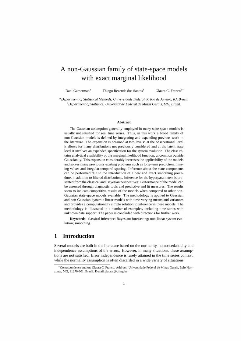
Figure 2 shows the RD series with its estimated smoothed means. The estimatesof the mean seem to follow better the behavior of the series with the NGSSM. Sum-mary measures based on fit and forecast errors are comparablebetween the two models,with a slight preference for the NGSSM. This improvement is probably due to betteradaptation to changes by the log-scaled beta disturbances.The figure also depicts theforecasts for future observations, based on a future scenario for the covariates and onthe results of Theorem 2. The forecasts seem to follow the behaviour of the smoothedmean values estimated at the end of the series, and the interval widths present an in-crease with the forecast horizon, as expected.
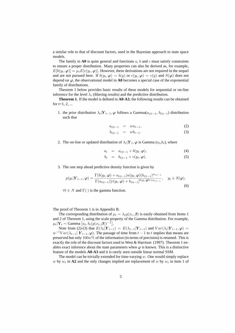
6.2 CEMIG return data
The second example refers to the daily data of CEMIG stock returns in the period from01/03/2005 to 06/08/2011 (1590 observations) and presentsseveral new models writtenin the NGSSM form, which do not belong to exponential family,like the Generalized
14

0 100 200 300 400
−20
12
34
t
Resid
uals
(a)
0 5 10 15 20 25
0.00.2
0.40.6
0.81.0
Lag
Resid
uals
(b)
0 100 200 300 400
−3−1
01
23
t
Resid
uals
(c)
0 5 10 15 20 25
0.00.2
0.40.6
0.81.0
Lag
ACF
(d)
Figure 1: Pearson and deviance residual analysis for the Poisson model. (a): time seriesof the Pearson residuals; (b): autocorrelation plot of the Pearson residuals; (c): timeseries of the deviance residuals; (d): autocorrelation plot of the deviance residuals.
gamma, Pareto with unknown scale parameter and Laplace withunknown mean mod-
els. Here the return at timet is defined asyt = ln(
Pt
Pt−1
), wherePt is the daily closing
spot price. The data irregularity due to holidays and weekends will be ignored. Figure3 presents the time series plot of the CEMIG returns. A distinctive feature of financialseries is that they usually present non-constant variance or volatility. This applicationillustrates the comparison of the fit of several observational distributions. For the anal-ysis of the CEMIG series, a temporal correlation structure is assumed for the varianceand two approaches are considered. In the first one, the Normal and Laplace models arefitted to the CEMIG returnsyt. In the second, the square transformationy2t is used, sothat Generalized Gamma, Gamma, Pareto and Inverse Gaussianmodels (with supportas the positive line) listed in Table 1 can be fitted to the series.
The Inverse Gaussian model was suggested by Barndorff-Nielsen & Shephard (2001)for modeling volatility series. Lopes & Migon (2002) used the Generalized gammamodel for modelling volatility series and Achar & Bolfarine(1986) utilized this log-linear model in survival analysis. The pareto model is well-known in the literature formodelling extreme events.
Table 3 shows the log-likelihood, AIC and BIC for the classical fits, and the DICcriterion for the Bayesian fits. For a fair comparison between the models, the log-likelihood in the second approach is corrected by the Jacobian of the transformation.The results show that the fit criteria discard the Inverse Gaussian model. The remainingmodels are somewhat comparable with a slight preference forthe Generalized gammamodel.
Table 4 shows the point and interval estimates for the parameters of the Generalizedgamma model. It can be seen that classical and Bayesian estimates are very similar.The residual analysis did not present any indication of model inadequacy (see Figure4).
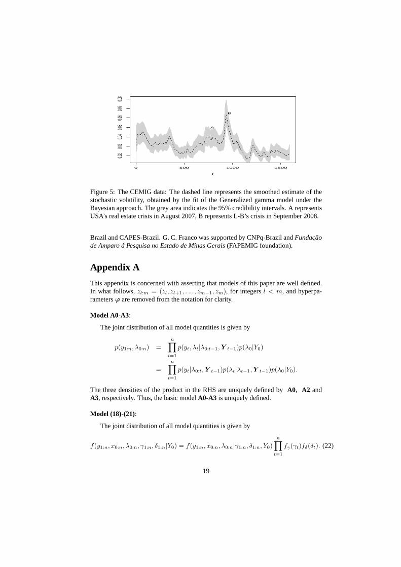
For illustration, Figure 5 shows the graph of the volatilityobtained by the General-
15
300 320 340 360 380 400
010
2030
40
t
Number
300 320 340 360 380 400
010
2030
40
t
Number
300 320 340 360 380 400
010
2030
40
t
Number
°°°°°°°°°°++++++++++
Figure 2: The full, dashed and dotted lines represent, respectively, the last 100 ob-servations of RD time series, the smoothed mean of the Bayesian estimation obtainedthrough the NGSSM approach and the smoothed mean obtained through the DGLMapproach. The vertical line separates the fitted data pointsfrom the forecast horizon.NGSSM mean: o; NDPSSM mean: +; NGSSM 95% interval limits:−−−.
t
Return
0 500 1000 1500
−0.10
−0.05
0.00
0.05
0.10
Cemig
Figure 3: CEMIG return series.
ized gamma model under the Bayesian approach. The peaks, corresponding to periodsof crisis known in the literature, can be observed in the figure, and are pointed out bythe model.
6.3 The Candy data
This section illustrates the application of dynamic linearmodels with non-Gaussiandisturbances and time-varying means and variances. Posterior samples of the staticand dynamic parameters are easily obtained for the model below using the approach ofSection 5. The Candy data, presented in Figure 6, is a well-known time series intro-duced in West & Harrison (1997, p. 331) and used for illustration of many featuresin that book. They consist on the monetary values of monthly total sales, on a stan-dardized, deflated scale, of a widely consumed and established food product in theUK market. The series is composed of 72 monthly observationsin the period from
16

Table 3: Values of log-likelihood, AIC, BIC and DIC for the models fitted to theCEMIG return.
Models log-likelihood AIC (c) BIC (c) DIC (b)
Generalized Gamma 3929.03 -4.94 -4.93 -7852.10Gamma 3928.00 -4.94 -4.93 -7852.00Normal 3926.00 -4.93 -4.93 -7850.00Laplace 3863.74 -4.86 -4.85 -7725.80Pareto 3639.53 -4.86 -4.85 -6517.00
Inverse Gaussian 2629.25 -3.31 -3.30 -5256.25
Note: (c) classical fit.(b) Bayesian fit.
Table 4: Point and interval (level 95%) estimation for the Generalized gamma modelfitted to the CEMIG series.
ϕ MLE Conf. Int. Posterior mean Cred. Int.w 0.941 [0.930; 0.960] 0.940 [0.920; 0.957]χ 0.397 [0.310; 0.484] 0.407 [0.332; 0.506]ν 1.135 [0.948; 1.321] 1.124 [0.952; 1.300]
01/1976 to 12/1981. The Index covariate is included in the analysis for explaining par-tial movements of the series. This index is built based on market prices, distributionand production costs.
As illustration, the model defined in Section 5 is fitted to theseries, assumingFt =
( 1 xt ), Gt =
(1 00 1
), xt =
(µt
βt
), wt =
(ηtξt
)andW =
(σ2η 00 σ2
ξ
).
This model is a local level model for time-varying interceptand regression coefficient.G(1.5,1.5) distributions are specified forγt’s and δt’s in order to obtain thet3-
Student errors for the observation and system disturbances. The number of degrees offreedomν is known, but can also be estimated (Fonseca, Ferreira & Migon, 2008).
The parameterw is fixed at 0.98 and initial values arem0 =
(9.5−0.7
), P0 =
(0.1 00 0.1
), a0 = 0.1 andb0 = 0.1, as suggested in West, Harrison & Pole (1987,
p. 333).Figure 6 presents the results of the estimation, where the smoothed mean responses
follow well the behavior of the series.Figure 7 shows smoothed estimates of the non-observable components fitted to the
series. The level componentµt oscillates in time in the early part of the series tocompensate seasonal effects whileβt decreases over time andλ−1
t shows a discretedecline.
Figure 8 summarizes estimation of hyperparameters and the time-varying scales.The posterior mean of the variance parameters are 1.11 and 1.10, respectively and theirdistributions are slightly asymmetric, as expected.
17

0 500 1000 1500
−4−3
−2−1
01
2
t
Resid
uals
(a)
0 5 10 15 20 25 30 35
0.00.2
0.40.6
0.81.0
Lag
ACF
(b)
0 5 10 15 20 25 30 35
0.00.2
0.40.6
0.81.0
Lag
ACF
(c)
0 5 10 15 20 25 30 35
−0.06
−0.02
0.02
Lag
Partial
ACF
(d)
Figure 4: Deviance residual analysis for the Gamma model. (a): time series of thedeviance residuals; (b): autocorrelation plot of the deviance residuals; (c): autocorrela-tion plot of the square of the deviance residuals; (d): partial autocorrelation plot of thesquare of the deviance residuals.
7 Discussion
Several possibilities of related future work can be thoughtof. Studies exploring proper-ties of the family of observational models inA0 and of special cases in this class can bemade. For example, the piecewise exponential distribution(Gamerman , 1994), whichhas a wide field of applications in reliability and survival analysis, may be adaptedto these non-Gaussian models. More general evolution equations with stationary andnon-stationary autoregressive structures may be proposed. Hypothesis tests can beexplored, as well as the use and application of the bootstraptechnique for making in-ference about the parameters. Extension towards non-Gaussian multivariate time seriesalong the lines set by Uhlig (1994) could also be entertained.
The existence of easily available procedures for inferenceis an attractive featureof these models. This is particularly relevant for use in time-varying components oflarger, more complex models. These components are typically latent and precise quan-titative assessments for them are usually not available. Qualitative assessments are thebasis for their probabilistic specifications. Availability of the mathematically tractableoptions may play an important role in the decision, when facing options that are equallyacceptable. This point was illustrated in Section 5.
The models are applicable to situations with fixed effects ofthe covariates. Animportant research development is the extension towards time-varying regression coef-ficients as considered in dynamic generalized linear models, but without losing analytictractability.
Acknowledgements
D. Gamerman was supported by CNPq-Brazil andFundacao de Amparoa Pesquisa noEstado do Rio de Janeiro(FAPERJ foundation). T. R. Santos was supported by CNPq-
18
t
0 500 1000 1500
0.02
0.03
0.04
0.05
0.06
0.07
0.08
B
A
Figure 5: The CEMIG data: The dashed line represents the smoothed estimate of thestochastic volatility, obtained by the fit of the Generalized gamma model under theBayesian approach. The grey area indicates the 95% credibility intervals. A representsUSA’s real estate crisis in August 2007, B represents L-B’s crisis in September 2008.
Brazil and CAPES-Brazil. G. C. Franco was supported by CNPq-Brazil andFundacaode Amparoa Pesquisa no Estado de Minas Gerais(FAPEMIG foundation).
Appendix A
This appendix is concerned with asserting that models of this paper are well defined.In what follows,zl:m = (zl, zl+1, . . . , zm−1, zm), for integersl < m, and hyperpa-rametersϕ are removed from the notation for clarity.
Model A0-A3:
The joint distribution of all model quantities is given by
p(y1:n, λ0:n) =n∏
t=1
p(yt, λt|λ0:t−1,Y t−1)p(λ0|Y0)
=
n∏
t=1
p(yt|λ0:t,Y t−1)p(λt|λt−1,Y t−1)p(λ0|Y0).
The three densities of the product in the RHS are uniquely defined by A0, A2 andA3, respectively. Thus, the basic modelA0-A3 is uniquely defined.
Model (18)-(21):
The joint distribution of all model quantities is given by
f(y1:n, x0:n, λ0:n, γ1:n, δ1:n|Y0) = f(y1:n, x0:n, λ0:n|γ1:n, δ1:n, Y0)
n∏
t=1
fγ(γt)fδ(δt). (22)
19

Year
1976 1977 1978 1979 1980 1981 1982
46
810
12
Figure 6: The full and dashed lines represent the series and the smoothed mean esti-mate, obtained by the fit under the Bayesian approach. The grey area indicates the 95%credibility intervals.
Year
1976 1978 1980 1982
78
910
12
µt
Year
1976 1978 1980 1982
−1.4
−1.0
−0.6
−0.2
βt
Year
1976 1978 1980 1982
02
46
8
λt
Year
1976 1978 1980 1982
0.01.0
2.03.0
γtλt−1
Figure 7: The smoothed estimates of dynamic components. Topleft: smoothed esti-mate of the level (µt); Top right: smoothed estimate of the regression coefficient (βt);Bottom left: smoothed estimate of the precision (λt); Bottom right: smoothed estimateof the variance (γtλ
−1t ).
20

Freque
ncy
0.0 1.0 2.0 3.0
0200
0400
0
(a)
Freque
ncy
0.0 1.0 2.0 3.0
0500
1500
2500
(b)
Year
1976 1978 1980 1982
1.04
1.08
1.12
(c)
Year
1976 1978 1980 1982
1.15
1.25
1.35
1.45
(d)
Figure 8: Posterior estimates: (a) - posterior histogram ofσ2η; (b) - posterior histogram
of σ2ξ ; (c) - smoothed means ofγt; (d) - smoothed means ofδt. Vertical dashed lines
indicate the posterior means.
But f(y1:n, x0:n, λ0:n|γ1:n, δ1:n, Y0) =
n∏
t=1
f(yt, xt, λt|Y t−1, x0:t−1, λ0:t−1, γ1:n, δ1:n)f(x0|Y0)f(λ0|Y0) (23)
and the joint densitiesf(yt, xt, λt|Y t−1, x0:t−1, λ0:t−1, γ1:n, δ1:n) can be decomposedas
f(yt|Y t−1, x0:t, λ0:t)f(λt|λ0:t−1,Y t−1, x0:t)f(xt|x0:t−1,Y t−1) =
f(yt|Y t−1, xt, λt)f(λt|λt−1,Y t−1, x0:t)f(xt|xt−1,Y t−1), (24)
where the dependence on(γ1:n, δ1:n) was removed from all terms in (24) for concise-ness. The densities in the RHS of (24) correspond to model specifications (18), (19) and(20), respectively, whereas the prior distributions (21) for the latent state componentsare provided in (23) and the mixing distributions are provided in (22). So, each modelcomponent in the distribution of(y1:n, x0:n, λ0:n, γ1:n, δ1:n|Y0) is uniquely defined.
Appendix B
This appendix presents the proof of the theorems provided inthe text. For ease ofnotation, hyperparameter vectorϕ will be omitted from the proofs.
Proof of Theorem 1.
In what follows, proofs of Results 1 to 3 from Theorem 1 are provided. In order toprove the theorem, the following lemma is needed.
21

Lemma. λt|λt−1,Yt−1 has density
p(λt|λt−1,Yt−1) =
kw
λt−1
(wλt
λt−1
)wat−1−1 (1−
wλt
λt−1
)(1−w)at−1−1
,
if 0 < λt < w−1λt−1,0, otherwise.
(25)
wherek =Γ(wat−1)Γ((1− w)at−1)
Γ(at−1).
Proof: The proof is easily obtained by using the Jacobian method and assumptionA2in Section 2 forh = 0.
Proof of Result (1) in Theorem 1:Assume by the induction hypothesis thatλt−1|Y t−1 ∼ Gamma (at−1, bt−1) and thedistribution ofλt = w−1λt−1ςt is given in Equation (25). Then,
p(λt|Y t−1) =
∫p(λt−1|Y t−1)p(λt|λt−1,Y t−1)dλt−1
=
∞∫
wλt
[λat−1−1t−1 exp(−bt−1λt−1)
Γ(at−1)b−at−1
t−1
]wλ−1
t−1(wλt
λt−1)wat−1−1(1− wλt
λt−1)(1−w)at−1−1
Γ(wat−1)Γ((1−w)at−1)Γ(at−1)
dλt−1
∝
∞∫
wλt
[λat−1−1−wat−1+1−1t−1 exp(−bt−1λt−1)
] [(1−
wλt
λt−1)(1−w)at−1−1
]dλt−1
∝
∞∫
wλt
[λ(1−w)at−1−1t−1 exp(−bt−1λt−1)
] [(1−
wλt
λt−1)(1−w)at−1−1
]dλt−1
∝
∞∫
wλt
exp(−bt−1λt−1)(λt−1 − wλt)(1−w)at−1−1dλt−1
.
=λwat−1−1t exp(−wbt−1λt)
(wbt−1)−wat−1Γ(wat−1), for λt > 0.
This is the density of aGamma(wat−1, wbt−1) distribution, completing the proof ofResult 1.
Proof of Result (2) in Theorem 1:By Bayes theorem,
p(λt|Y t,ϕ) ∝ p(yt|λt,ϕ)p(λt|Y t−1,ϕ) ∝λ(at|t−1+b(yt,ϕ))−1t exp[−λt(bt|t−1+c(yt,ϕ))].
Then, it follows thatλt|Y t,ϕ ∼ Gamma (at, bt), whereat = at|t−1 + b(yt,ϕ)andbt = bt|t−1+c(yt,ϕ), completing the induction. Sinceλ0|Y 0,ϕ ∼ Gamma (a0, b0),
22
the proof is complete, for allt.
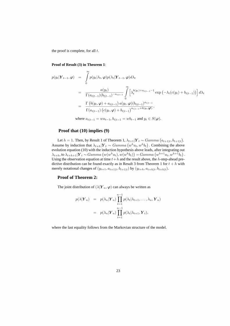
Proof of Result (3) in Theorem 1:
p(yt|Y t−1,ϕ) =
∞∫
0
p(yt|λt,ϕ)p(λt|Y t−1,ϕ)dλt
=a(yt)
Γ(at|t−1)(bt|t−1)−at|t−1
∞∫
0
[λb(yt)+at|t−1−1t exp
(−λt(c(yt) + bt|t−1)
)]dλt
=Γ(b(yt,ϕ) + at|t−1
)a(yt,ϕ)(bt|t−1)
at|t−1
Γ(at|t−1)(c(yt,ϕ) + bt|t−1
)at|t−1+b(yt,ϕ),
whereat|t−1 = wat−1, bt|t−1 = wbt−1 andyt ∈ S(ϕ).
Proof that (10) implies (9)
Let h = 1. Then, by Result 1 of Theorem 1,λt+1|Y t ∼ Gamma(at+1|t, bt+1|t
).
Assume by induction thatλt+h|Y t ∼ Gamma(what, w
hbt). Combining the above
evolution equation (10) with the induction hypothesis above leads, after integrating outλt+h, toλt+h+1|Y t ∼Gamma
(w(what), w(w
hbt))=Gamma
(wh+1at, w
h+1bt).
Using the observation equation at timet+h and the result above, theh-step-ahead pre-dictive distribution can be found exactly as in Result 3 fromTheorem 1 fort+ h withmerely notational changes of(yt+1, at+1|t, bt+1|t) by (yt+h, at+h|t, bt+h|t).
Proof of Theorem 2:
The joint distribution of(λ|Y n,ϕ) can always be written as
p(λ|Y n) = p(λn|Y n)n−1∏
t=1
p(λt|λt+1, . . . , λn,Y n)
= p(λn|Y n)n−1∏
t=1
p(λt|λt+1,Y t),
where the last equality follows from the Markovian structure of the model.
23

The required density of[λt|λt+1,Y t] is given by
p(λt−1|λt,Y t−1) =p(λt|λt−1,Y t−1)p(λt−1|Y t−1)
p(λt|Y t−1)
=Γ(wat−1)Γ((1− w)at−1)
Γ(at−1)
w
λt−1
(wλt
λt−1
)wat−1−1(1−
wλt
λt−1
)(1−w)at−1−1
×
bat−1
t−1
Γ(at−1)λat−1−1t−1 exp(−λt−1bt−1)
Γ(wat−1)(wbt−1)
wat−1
λwat−1−1t exp(−λtwbt−1)
∝ (λt−1 − wλt)(1−w)at−1−1 exp (−bt−1(λt−1 − wλt)) .
Now, defineηt−1 = λt−1 −wλt by removal of the constantwλt from λt−1. Then,p(ηt−1|λt,Y t−1) ∝ η
(1−w)at−1−1t−1 exp (−bt−1ηt−1) . It is clear thatηt−1 = λt−1 −
wλt|λt,Y t−1 ∼ Gama((1− w)at−1, bt−1), completing the proof.
References
ACHAR, J. & BOLFARINE, H. (1986). The log-linear model with a generalized gammadistribution for the error: a Bayesian apporach.Stat. Prob. Lett.4, 325–332.
ALVES, M. B., GAMERMAN , D. & FERREIRA, M. A. R. (2010). Transfer functionsin dynamic generalized linear models.Stat. Model.10, 3–40.
ARNOLD, B. C. & PRESS, S. J. (1989). Bayesian estimation and prediction for paretodata.J. Amer. Statist. Assoc.84, 1079–1084.
ANDRIEU, C. & DOUCET, A. (2002). Particle filtering for partially observed Gaussianstate space models.J. R. Statist. Soc.B 64, 827–836.
BARNDORFF-NIELSEN, O. E. & SHEPHARD, N. (2001). Non-Gaussian Ornstein-Uhlenbeck based models and some of their uses in financial economics (with dis-cussion).J. R. Statist. Soc.B 63, 167–241.
CARLIN , B.P., POLSON, N.G. & STOFFER, D.S. (1992). A Monte Carlo approach tononnormal and nonlinear state-space modeling.J. Amer. Statist. Assoc.87, 493-500.
CARTER, C. K. & KOHN, R. (1994). On Gibbs sampling for state space models.Biometrika81, 541–553.
CARVALHO , C. M., JOHANNES, M. S., LOPES, H. F. & POLSON, N. G. (2010).Particle Learning and Smoothing.Statist. Sci.25, 88–106.
CASELLA , G. & BERGER, R. L. (2002).Statistical Inference. (2nd edition). Michi-gan: Thomson Learning.
CAVANAUGH , J. E. & SHUMWAY, R. H. (1996). On computing the expected Fisherinformation matrix for state-space model parameters.Statist. Probab. Lett.26, 347–355.
24

CHIOGNA, M. & GAETAN , C. (2002). Dynamic generalized linear models with ap-plication to environmental epidemiology.Appl. Statist.51, 453–468.
DETHLEFSEN, C. & LUNDBYE-CHRISTENSEN, S. (2006). Formulating state spacemodels in R with focus on longitudinal regression models.J. Statist. Software16,1–15.
DURBIN, J. & KOOPMAN, S. J. (2001).Time Series Analysis by State Space Methods.Oxford:Oxford University Press.
FAHRMEIR, L. & K AUFMANN , H. (1987). Regression models for non-stationary cat-egorical time series.J. Time Series Anal.8, 147–160.
FAHRMEIR, L. & T UTZ, G. (2001).Multivariate statistical modelling based on gen-eralized linear models. Springer: New York.
FERRIS, B. G., DOCKERY, D. W., WARE, J. H., SPEIZER, F. E. & SPIRO, R. (1983).The six-city study: examples of problems in analysis of the data. EnvironmentalHealth Perspectives52, 115–123.
FONSECA, T. C. O., FERREIRA, M. A. R. AND M IGON, H. S. (2008). ObjectiveBayesian analysis for the Student-t regression model.Biometrika95, 325–333.
FRANCO, G. C., SANTOS, T. R., RIBEIRO, J. A. & CRUZ, F. R. B. (2008). Confi-dence intervals for hyperparameters in structural models.Comm. Statist. SimulationComput.37, 486–497.
FRUHWIRTH-SCHNATTER, S. (1994). Applied state space modelling of non-Gaussiantime series using integration-based Kalman filtering.Stat. Comput.4, 259–269.
FRUHWIRTH-SCHNATTER, S. & WAGNER, H. (2006). Auxiliary mixture samplingfor parameter-driven models of time series of counts with applications to state spacemodelling.Biometrika93, 827–841.
GAMERMAN , D. (1991). Dynamic Bayesian models for survival data.Appl. Statist.40, 63–79.
GAMERMAN , D. (1994). Bayes estimation of the piece-wise exponentialdistribution.IEEE Trans. Reliab.43, 128–131.
GAMERMAN , D. (1998). Markov chain Monte Carlo for dynamic generalised linearmodels.Biometrika85, 215–227.
GAMERMAN , D. & L OPES, H. F. (2006). Markov Chain Monte Carlo: StochasticSimulation for Bayesian Inference. (2nd edition). London: Chapman and Hall.
GELMAN , A. (1996).Inference and monitoring convergence.In Markov Chain MonteCarlo in Practice. W.R. Gilks, Richardson, S. Spiegelhalter, D. J. (eds). London:Chapman and Hall, pp. 131-143.
25

GODOLPHIN, E. J. & TRIANTAFYLLOPOULOS, K. (2006). Decomposition of timeseries models in state-space form.Comput. Statist. Data Anal.50, 2232–2246.
GRUNWALD , G. K., RAFTERY, A. E. & GUTTORP, P. (1993). Time series of contin-uous proportions.J. R. Statist. Soc.B 55, 103–116.
HAIGHT, F. A. & BREUER, M. A. (1960). The Borel-Tanner Distribution.Biometrika47, 143–150.
HARVEY, A.C. (1989). Forecasting, Structural Time Series Models and the KalmanFilter. Cambridge: Cambridge University Press.
HARVEY, A. C. & FERNANDES, C. (1989). The time series models for count orqualitative observations.J. Bus. Econom. Statist.7, 407–417.
JACQUIER, E., POLSON, N. G. & ROSSI, P. E. (1994). Bayesian analysis of stochasticvolatility models.J. Bus. Econom. Statist., 12, 371-389.
K IM , S., SHEPHARD, N. & CHIB , S. (1998). Stochastic volatility: likelihood infer-ence and comparison with ARCH models.Rev. Econom. Stud., 65, 361-93.
L INDSEY, J. K. & LAMBERT, P. (1995). Dynamic generalized linear-models andrepeated measurements.J. Statist. Plann. Inference47, 129–139.
LOPES, H. F. & M IGON, H. S. (2002).Comovements and contagion in emergent mar-kets: stock indexes volatilities.In: C. Gatsonis, R. Kass, A. Carriquiry, A. Gelmanand D. Higdon (Eds.), Case Studies in Bayesian Statistics, Volume VI (p. 285-300).New York: Springer-Verlag.
M IGON, H. S. & GAMERMAN , D. (1999). Statistical Inference: An Integrated Ap-proach. London: Arnold.
M IGON, H. S., GAMERMAN , D., LOPES, H. F. & FERREIRA, M. A. R. (2005).Dynamic models.In: Handbook of Statistics - Bayesian Thinking, Modeling andComputation. Dipak K. Dey and C. R. Rao (Eds). Amsterdam: Elsevier, pp. 553-588.
MCCULLAGH , P. & NELDER. J. A. (1989).Generalized Linear Models. New York:Chapman and Hall.
NELDER. J. A. & WEDDERBURN, R. W. M. (1972). Generalized linear models.J.R. Statist. Soc.A 135, 370–384.
NOCEDAL, J. & WRIGHT, S. J. (2006).Numerical Optimization (2nd ed.). New York:Springer-Verlag.
PITT, M. K. & WALKER , S. G. (2005). Constructing stationary time series modelsusing auxiliary variables with applications.J. Amer. Statist. Assoc.100, 554–564.
SALLAS , W. M. & H ARVILLE , D. A. (1988). Noninformative priors and restrictedmaximum likelihood estimation in the Kalman filter.Bayesian Analysis of TimeSeries and Dynamic Models, J. C. Spall (Ed). New York:Marcel Dekker Inc.
26
SHEPHARD, N. (1994). Local scale models: state space alternative to integratedGARCH processes.J. Econometrics60, 181–202.
SHEPHARD, N. & PITT, M. K. (1997). Likelihood analysis of non-Gaussian measure-ment time seriesBiometrika84, 653–667.
SILVA , R. S., LOPES, H. F. & M IGON, H. S. (2006). The extended generalizedinverse Gaussian distribution for log-linear and volatility models. Braz. J. Prob.Stat.B 20, 67–91.
SMITH , R. L. & M ILLER , J. E. (1986). A non-Gaussian state space model andapplication to prediction of records.J. R. Statist. Soc.B 48, 79–88.
SPIEGELHALTER, D. J., BEST, N. G., CARLIN , B. P. & VAN DER L INDE, A. (2002).Bayesian measures of model complexity and fit (with discussion). J. R. Statist. Soc.B 64, 583–639.
UHLIG , H. (1994). On singular Wishart and singular multivariate beta distributions.Ann. Statist.22, 395-405.
WEST, M. (1987). On scale mixtures of normal distributions.Biometrika, 74, 646-648.
WEST, M. & H ARRISON, P. J. (1997).Bayesian Forecasting and Dynamic Models.New York: Springer.
WEST, M., HARRISON, P. J. & MIGON, H. S. (1985). Dynamic generalized linearmodels and Bayesian forecasting (with discussion)J. Amer. Statist. Assoc.80, 73–97.
WEST, M., HARRISON, P.J. & POLE, A. (1987). BATS: Bayesian analysis of timeseries.The Professional Statistician, 6, 43-46.
27