a note on the error in gaussian quadrature

A Note on the Error in Gaussian Quadrature

Clyde Martin* and Mark Stamp’

Department of Mathematics Texas Tech University Lubbock, Texas 79409

ABSTRACT

The error in Gaussian quadrature is analyzed using methods from the theory of

analytic functions. It is well known that the error term may be expressed in terms

of a contour integral against a kernel function K,(t). We give two methods for

computing the coefficients (in terms of the moments) for the Laurent series of

K,(t), and we give explicit expressions for K,(t) for two particular measures. We

then use the Laurent expansion of K,(t) to estimate the error for various functions

and measures.

1. INTRODUCTION

In this paper we examine the error in Gaussian quadrature in the case where the integrand is an analytic function and the interval of integration is finite. In Section 2 we give a well-known representation for the error as a contour integral against a kernel function K,(t), and we show that under certain further restrictions, K,(t) has a valid Laurent series expansion. We then develop two methods for computing the coeflicients (in terms of the moments) of the resulting Laurent series. Section 3 gives a method for finding an explicit expression for K,(t), which is then used to compute K,(t) for two specific measures. Finally, in Section 4 we apply the methods of Section 2 to estimate the error that occurs when various Gaussian quadrature rules are applied to particular functions.

*Supported in part by NASA grant NAG%89, NSF grant DMS 8905334 and NSA grant MDA904-90-H-4009. ‘Supported in part by NSA grant MDA904-90-H-4009.

APPLlED MATHEMATICS AND COMPUTATION 47:25-35 (1992)

0 Elsevier Science Publishing Co., Inc., 1992 655 Avenue of the Americas, New York, NY 10010

25

0096-3003/92/$03.50

26 CLYDE MARTIN AND MARK STAMP

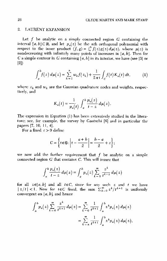
2. LAURENT EXPANSION

Let f be analytic on a simply connected region G containing the interval [a, b] C W, and let p,(z) be the nth orthogonal polynomial with respect to the inner product (f, g) = 1," f( z)g( z) dp( z), where /J(Z) is nondecreasing with infinitely many points of increases in [a, b]. Then for C a simple contour in G containing [a, b] in its interior, we have (see [3] or

PI)

where ‘- AJk and wk are the Gaussian quadrature nodes and weights, respec- tively, and

1 Kn( t) = - J b Pn( x)

p,(t) a ,,W).

The expression in Equation (1) has been extensively studied in the litera- ture; see, for example, the survey by Gautschi [6] and in particular the papers [7, 10, 11, 41.

For a fixed E > 0 define

we now add the further requirement that f be analytic on a simple connected region G that contains C. This will insure that

for all z E[ a, b] and all t EC, since for any such z and t we have 1 z/t 1 Cl. NOW for tEC fixed, the sum C,“=, zk/tk+’ is uniformly convergent on [a, b], and hence

Gaussian Quadrature 27

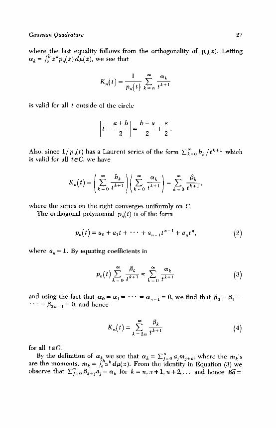
where the last equality follows from the orthogonality of p,(z). Letting ok = jab z ‘p,( z) dp( z), we see that

is valid for all t outside of the circle

a+b b-a E I I t-- 2

=-+- 2 2’

Also, since l/p,(t) has a Laurent series of the form C,“=, bk / tk+’ which is valid for all teC, we have

where the series on the right converges uniformly on C. The orthogonal polynomial p,(t) is of the form

p,(t) = a,+a,t+ *a* +a,_,t”-‘+a,t”,

where a,, = 1. By equating coeffkients in

(2)

and using the fact that CY~ = err = * - + = (Y,_ r = 0, we find that PO = fll = . . . = &_r = 0, and hence

(4)

for all teC. By the definition of (Y& we see that ok = Cj”=, ajmj+&, where the mk’s

are the moments, m& = Jabzk dp( z). From the identity in Equation (3) we observe that C~z,Pk+jaj=cx& for k=n,:z+l,n+&... and hence Bz=


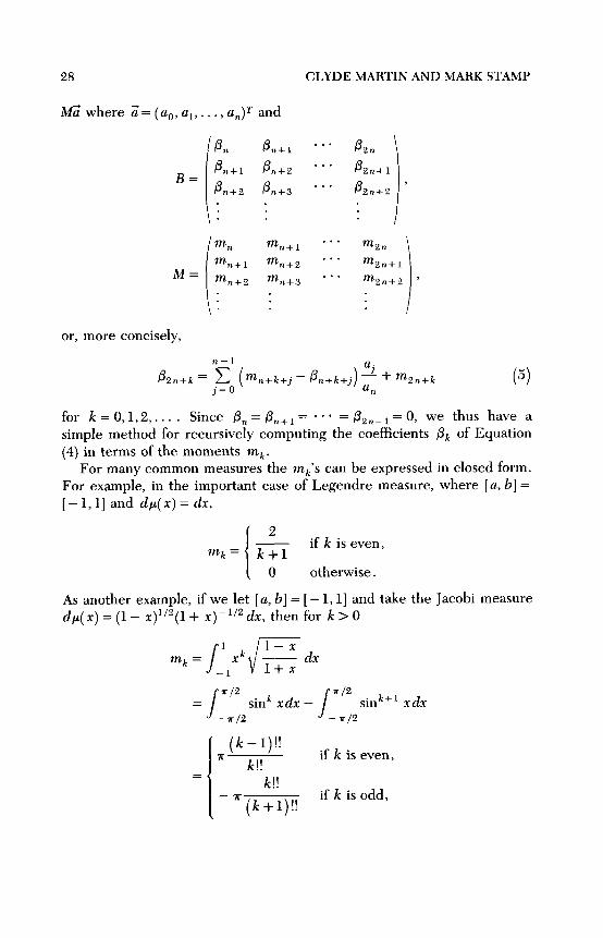
Xi where si= (a,, al,. . . , u,)T and

B=

M=

or, more concisely,

kL PiIf1 *** fl2n P n+l on+2 *** PZn+l P n+2 on+3 *** P2”+2

.

m, m m n+l m

:: i

n+l *** mzn n+2 *** mzn-

m n+2 m ?I+3 **- mzn-

i-1 I t2 ’

n-1

P 2n+k = JFo ( mn+k+j - fin+k+j): + m2n+k n

for k=0,1,2,... . Since fi,,=fi,+,= *** =P2n_1=0, we thus have a simple method for recursively computing the coefficients pk of Equation (4) in terms Of the moments mk.

For many common measures the mk’s can be expressed in closed form. For example, in the important case of Legendre measure, where [a, b] = [ - 1, l] and dp( x) = dx,

- if k iseven,

otherwise.

As another example, if we let [a, b] = [ - 1, l] and take the Jacobi measure dp( X) = (1 - x)l/‘(l+ x)-1/z&, then for k > 0

mk=/:lxk/zdx

= s

*P sink xdx -

- r/z J

*I2 sink+’ xdx

- *I2

i

7rck+ k!!

if k is even,

= k!!

-K(~+~)!! if k isodd,


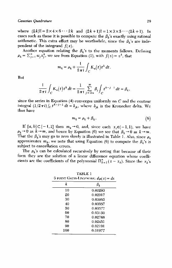
where (Zk)!!=2~4~6*.* 2k and (2k+l)!!=lx3x5***(2k+l). In cases such as these it is possible to compute the ok’s exactly using rational arithmetic. This extra effort may be worthwhile, since the ok’s are inde- pendent of the integrand f(x).

Another equation relating the ok’s to the moments follows. Defining pk = Cy= i wjx:, we see from Equation (1) with f(z) = ,zk, that

But

1 -1 K,(t)tkdt= 27ri c

& ,$ bj J tk-jpl dt = ok> 3 n c since the series in Equation (4) converges uniformly on C and the contour integral (1/2?ri)/c tk-j-’ dt = cSjk,

thus have where 6jk is the Kronecker delta. We

mk=pk+&. (6)

If [a,b]c[-l,l] th en mk+O, and, since each xi~( - 1, l), we have pk + 0 as k +a, and hence by Equation (6) we see that fik + 0 as k + co.

That the ok’s may go to zero slowly is illustrated in Table 1. Also, since pk approximates mk, we note that using Equation (6) to compute the @k’s is subject to cancellation errors.

The pk’s can be calculated recursively by noting that because of their form they are the solution of a linear difference equation whose coefficients are the coefficients of the polynomial I-I;= 1 (x - xk). Since the xk’s

TABLE1 5 POINT GAUSS-LEGFNDRE: dp( r) = dx

k Pk

10 0.00293

20 0.02917 30 0.03985 40 0.03957 50 0.03577 60 0.03150 70 0.02768 80 0.02451 90 0.02191 100 0.01977


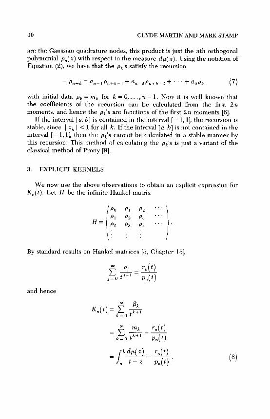
are the Gaussian quadrature nodes, this product is just the nth orthogonal polynomial p,(x) with respect to the measure dp( x). Using the notation of Equation (2), we have that the pk’s satisfy the recursion

- &+k = an-l&+k-l + an-2&,+k-2 + * ” + aopk (7)

with initial data pk = mk for k = 0,. . . , n - 1. Now it is well known that the coefficients of the recursion can be calculated from the first 2n moments, and hence the pk’s are functions of the first 2n moments [6].

If the interval [a, b] IS contained in the interval [ - 1, 11, the recursion is stable, since 1 xk 1 C 1 for all k. If the interval [a, b] is not contained in the interval [ - 1, lb then the pk’s cannot be calculated in a stable manner by this recursion. This method of calculating the pk’s is just a variant of the classical method of Prony [q].

3. EXPLICIT KERNELS

We now use the above observations to obtain an explicit expression for K,(t). Let H be the infinite Hankel matrix

H=

I

PO Pl Pz *-* Pl P2 P, *-*

Pz P3 P4 *** . . . . . . . . .

By standard results on Hankel matrices [5, Chapter 151,

and hence

4t) =k~oz+qq

s bb( z) rdt) = -- ~ t--z p,(t)

(8)


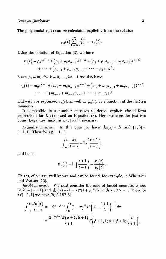
The polynomial r,(t) can be calculated explicitly from the relation

Using the notation of Equation (2) we have

r,(t) = p,t”_1 + (PI + POql)t”-2 + (P2 + Plan-l + POa”-2)t”-3

+ *** +(P,-l+P,-za,_l+ *** +p,ap.

Since pk=mk for k=O,...,2n-1 we also have

r,(t) = motnpl + (m, + mOanpl ) t”-’ + ( m2 + m,u,_, + mOun_2) tnp3

+ ..* +(m,_, +m,_,u,_,+ *** +m,u,)t’

and we have expressed r,(t), as well as p,(t), as a function of the first 2 n moments.

It is possible in a number of cases to derive explicit closed form expressions for K,(t) based on Equation (8). Here we consider just two cases: Legendre measure and Jacobi measure.

Legendre measure. In this case we have dp( x) = dx and [a, b] = [-l,l]. Then for t$[-l,l]

J 1 dr

-= _,t- x

and hence

t+1 K,(t)=ln t_l --

i i

r4t)

p,(t) ’

This is, of course, well known and can be found, for example, in Whittaker and Watson [13].

uco i measure. We next consider the case of Jacobi measure, where [u,~]=~[-I,I] and dp(x)=(l- ~)~(l+ r)“dr with a,@>-1. Then for t$[ - 1, l] we have [B, 3.197.81

J 1 h(X) 1 _ = _2a+P+l t+1 -I

1 X aX@ x-- dx -1 t-x J

0

(4 ( 2 1

= 2”+B+‘qor+w3+1)F

t+1


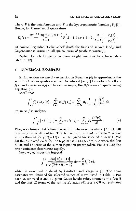
where B is the beta function and F is the hypergeometric function a F1 [l]. Hence, for Gauss-Jacobi quadrature

q t) = 2”+~+‘q~+Li3+qF p+l l a+P+2 2

i r4t) , ; .- --

t+1 ’ t+l 1 p,(t) .

Of course Legendre, Tschebysheff (both the first and second kind), and Gegenbauer measure are all special cases of Jacobi measure [3].

Explicit kernels for many common weight functions have been tabu- lated in [I2].

4. NUMERICAL EXAMPLES

In this section we use the expansion in Equation (4) to approximate the error in Gaussian quadrature over the interval [ - 1, l] for various functions f(x) and measures dp( x). In each example, the ok’s were computed using Equation (5).

Recall that

or, since f is analytic,

First, we observe that a function with a pole near the circle 1 t ) = 1 will obviously cause difficulties. This is clearly illustrated in Table 2 where error estimates for f(x) = l/( x - (Y are given for selected (Y near 1. We ) list the estimated error for the 5 point Gauss-Legendre rule when the first 5, 10, and 15 terms of the sum in Equation (9) are taken. For CY < 1.25 the error estimates deteriorate rapidly.

Next, we consider the integral

J 1 cos[a(x+l)]

_1 J(3+ .r)(I- r) & = 5ja(2+

which is examined in detail by Gautschi and Varga in [7]. The error estimates we obtained for selected values of a are listed in Table 3. For each a, we used 5 and 10 point Gauss-Jacobi rules, summing the first 5 and the first 12 terms of the sum in Equation (9). For a < 8 our estimates

GaussMn Quadrature 33

TABLE 2 5 POINT GAUSS-LEGENDRE: dp( x) = dx

f(x) True error

Error estimates (number of terms)

5 10 15

1 - 1.01016263 -

X - 1.01 0.02159575 - 0.05870456 - 0.13604425

1 - 0.04236274 -

r -1.1 0.00666266 - 0.01460258 - 0.02547044

1 -

r-1.25 0.00283570 - 0.00117919 - 0.00197875 - 0.00257487

1

x-1.5 - 0.00014913 - 0.00010663 - 0.00013775 - 0.00014791

TABLE 3

n POINT GAUSS-JACOBI:

fCx) = cos[a(x +l)l ll5Ti

,dp(x)=(l- x)-“‘dr

Error estimates (no. of terms)

a n True error 5 12

0.5 5 3.9288E - 09 3.9387x - 09 3.9287E - 09 10 6.7300~ - 17 6.6656~ - 17 6.7294E - 17

1.0 5 - 4.3636~ - 09 -4.374lE-09 -4.3635E-09 10 - 6.3300~- 17 - 6.2747~ - 17 - 6.3315~~17

2.0 5 3.8809E-07 3.8805~-07 3.88093-07 10 7.0400E-17 -6.9715~-17 -7.0414E-17

4.0 5 7.6865~-05 8.2420~-05 7.6865~-05 10 5.98OOE-14 -6.0942~-14 -5.9820~-14

8.0 5 0.10516245 0.05655472 0.10358893 10 3.0113E-07 -2.9629E-07 -3.0105E-07

16.0 5 0.38154533 8023.61 -4695.45

10 0.03097828 -2.7543 0.2791

32.0 5 0.52130367 -1.4~08 1.6309

10 0.16326226 6.2~07 -3.6~08

are comparable to those obtained (using very different methods) in [7].

Obviously many more terms of the infinite series would be required in order to achieve any reasonable error estimates for larger values of a. This

is to be expected since in this particular example fck)(0) is growing like uk,


and hence for large values of a, k must become very large before fck)(0)/k! becomes manageable.

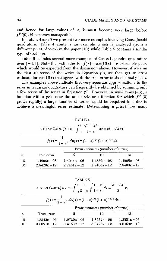
In Tables 4 and 5 we present two more examples involving Gauss-Jacobi quadrature. Table 4 contains an example which is analyzed (from a different point of view) in the paper [lo], while Table 5 contains a similar type of problem.

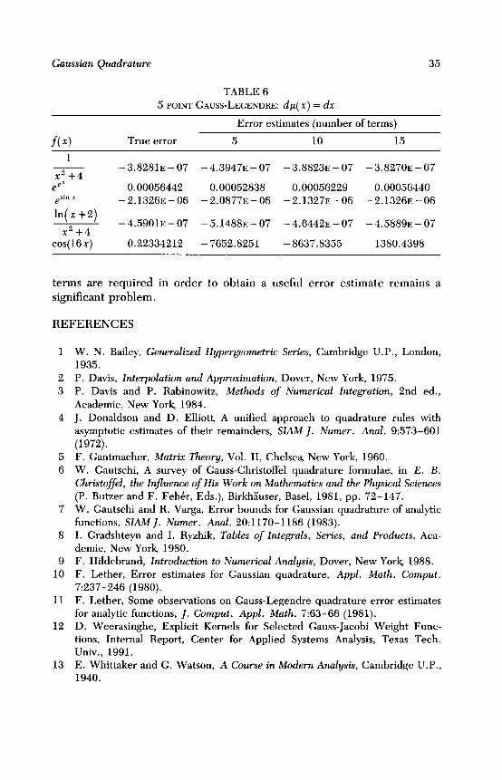
Table 6 contains several more examples of Gauss-Legendre quadrature over [ - 1, 11. Note that estimates for f(x) = cos(l6x) are extremely poor, which would be expected from the discussion above. However, if we sum the first 40 terms of the series in Equation (9), we then get an error estimate for cos(l6r) that agrees with the true error to six decimal places.

The examples above indicate that very accurate approximations to the error in Gaussian quadrature can frequently be obtained by summing only a few terms of the series in Equation (9). However, in some cases [e.g., a function with a pole near the unit circle or a function for which fck)(0) grows rapidly] a large number of terms would be required in order to achieve a meaningful error estimate. Determining a priori how many

TABLE 4

J 1dZ-F

TI POINT GAUSS-JACOBI: -1 2-x

dx=(Z- +r;

f(x)= $qT dp( x) = (1- x)@(l + ql” dx


n True error 5 10 15

5 l.4906E - 06 1.4044E - 06 1.4839E-06 l.4905E - 06

10 2.8420~ - 12 2.2461~ - 12 2.7466~ - 12 2.8400~ - 12

TABLE 5

nPoINTCAUSS-JACOBI: J:l&/zdx=vn:

f(x)= & dp( x) = (1 - x)l”( 1 + x) - “’ dx


n True error 5 10 15

5 1.8543~-06 l.g%oE - 06 1.8334~ - 06 1.8551~~06

10 3.50913 - 12 3.4153~ - 12 3.3472~ - 12 3.5459E - 12

35 Gaussian Quudrature

TABLE 6

5 POINT GAUSS-LEGENDRE: dp( x) = dx


f(x) True error 5 10 15

1

x2+4 -3.8281~-07 -4.3947E-07 -3.8823~-07 -3.8270~-07

e .= 0.00056442 0.00052838 0.00056229 0.00056440 sin x

1”,(x+2j

-2.1326~-06 -2.0877~-06 -2.1327~-06 -2.1326~~06

x2+4 -4.59OlE-07 -5.1488~-07 - 4.6442~ - 07 - 4.5889E - 07

cos(l6x) 0.22334212 - 7652.8251 - 8637.8355 1380.4398

terms are required in order to obtain a useful error estimate remains a

significant problem.

REFERENCES

4

5

6

7

8

9 10

11

12

13

W. N. Bailey, Generalized Hypergeometric Series, Cambridge U.P., London, 1935.

P. Davis, Znterpolation and Approximation, Dover, New York, 1975. P. Davis and P. Rabinowitz, Methods of Numerical Integration, 2nd ed.,

Academic, New York 1984. J. Donaldson and D. Elliott, A unified approach to quadrature rules with

asymptotic estimates of their remainders, SZAM 1. Numer. Anal. 9:573-601 (1972). F. Gantmacher, Matrix Theory, Vol. II, Chelsea, New York, 1960.

W. Gautschi, A survey of Gauss-Christoffel quadrature formulae, in E. B. Christoffel, the Znjluence of His Work on Mathematics and the Physical Sciences (P. Butzer and F. Fehdr, Eds.), Birkhzuser, Basel, 1981, pp. 72-147. W. Gautschi and R. Varga, Error bounds for Gaussian quadrature of analytic functions, SZAMJ. Numer. Anal. 20:1170-1186 (1983). I. Gradshteyn and I. Ryzhik, Tables of Integrals, Series, and Products, Aca- demic, New York 1980. F. Hildebrand, Zntroduction to Numerical Analysis, Dover, New York 1988. F. Lether, Error estimates for Gaussian quadrature, Appl. Math. Comput. 7:237-246 (1980). F. Lether, Some observations on Gauss-Legendre quadrature error estimates for analytic functions, 1. Comput. Appl. Math. 7:63-66 (1981). D. Weerasinghe, Explicit Kernels for Selected Gauss-Jacobi Weight Func- tions, Internal Report, Center for Applied Systems Analysis, Texas Tech. Univ., 1991. E. Whittaker and G. Watson, A Course in Modern Analysis, Cambridge U.P., 1940.

a note on the error in gaussian quadrature

Documents