A Note on the Estimation of theMultinomial Logistic Model with

Correlated Responses in SAS

Oliver Kuss

Institute of Medical Epidemiology, Biostatistics, and Informatics,

University of Halle-Wittenberg

06097 Halle (Saale), Germany

Phone: +49-345-5573582, Fax: +49-345-5573580

Email: Oliver.Kuss@medizin.uni-halle.de

Dale McLerran

Fred Hutchinson Cancer Research Center

1100 Fairview Ave N., M2-B230 P.O. Box 19024

Seattle, WA 98109-1024

Phone: (206) 667-2926, Fax: (206) 667-5977

Email: dmclerra@fhcrc.org

Abstract

We show how multinomial logistic models with correlated responses can

be estimated within SAS software. To achieve this, random effects and

marginal models are introduced and the respective SAS code is given.

An example data set on physicians’ recommendations and preferences in

traumatic brain injury rehabilitation is used for illustration. The main

motivation for this work are two recent papers that recommend estimating

multinomial logistic models with correlated responses by using a Poisson

likelihood which is statistically correct but computationally inefficient.

Keywords: Multinomial logistic model, random effects, marginal models,

SAS, GEE

Short title: Multinomial Logistic Models with Correlated Responses in

SAS

1 Introduction

Many study designs in applied sciences give rise to correlated data. For ex-

ample, subjects are followed over time, are repeatedly treated under different

experimental conditions, or are observed in logical clusters (e.g. clinics, fami-

lies, litters). In regression modelling, theory and methods for correlated data

are available for continuous responses, and also, despite enhanced mathematical

complexity, for binary responses. Less used have been models for the analy-

sis of multinomial responses. Some rare examples are Hartzel et al. [1], Rev-

elt/Train [2] in econometrics, and Hedeker [3], Skrondal/Rabe-Hesketh [4], and

Daniels/Gatsonis [5] in medicine and public health research.

In general, there are two large families of statistical models that may be

employed to account for the correlation structure, marginal and conditional (or

random effect) models. For non-Gaussian responses, estimated parameters have

different interpretations for each of these two model families [6]. In marginal

models, the mean function is modelled directly and the correlation structure

is regarded as a nuisance parameter. In random effect models, correlation is

introduced through shared random effects in the linear predictor.

Concerning estimation methods and software, Hartzel et al. [1] compare

different methods of estimation for random effect models with multinomial re-

sponses and consider adaptive Gauss-Hermite quadrature, penalized quasi likeli-

hood (PQL), an MCEM algorithm, and a non-parametric maximum likelihood

(NPMLE) method. Hartzel et al. [1] give SAS PROC NLMIXED code for

estimation of multinomial random effects models by adaptive Gauss-Hermite

3

quadrature. In econometrics, models with multinomial responses and random

effects are known under the heading of ’Mixed Logit’, as the response probabil-

ity is a mixture of logits with a specified, generally normal, mixing distribution

[2, 7]. The preferred estimation method seems to be simulated maximum like-

lihood for these models, a series of Gauss and MATLAB macros is available

from K. Train’s website [8]. Skrondal/Rabe-Hesketh [4] show how the multino-

mial model with random effects fits in their class of Generalized linear latent

and mixed models (GLLAMM) and describe how to use STATA for model fit-

ting. Hedeker [3] uses the idea of maximum marginal likelihood and supplies the

stand-alone software MIXNO [9] for parameter estimation. Daniels/Gatsonis [5]

propose a Bayesian approach (Gibbs sampling in combination with Metropolis

steps) for parameter estimation in multinomial random effects models.

Chen/Kuo [10] also show how to fit multinomial logistic models with random

effects. They used the well-known (see, e.g., [11]) relation between multinomial

and Poisson models to restate the multinomial logistic model with random ef-

fects as, alternatively, a Poisson log-linear model ([10], section 3.2) or a Poisson

nonlinear model ([10], section 3.3), each of them also with random effects. Using

the log-linear formulation, the model can be fitted with the SAS %GLIMMIX

macro (or the new experimental PROC GLIMMIX). The Poisson nonlinear

model can be estimated employing SAS PROC NLMIXED. The Poisson log-

linear model requires estimation of N =∑I

i=1 ni incidental parameters in ad-

dition to the model parameters, where I is the number of clusters, and ni is

the number of observations within clusters. Thus, the Poisson log-linear model

4

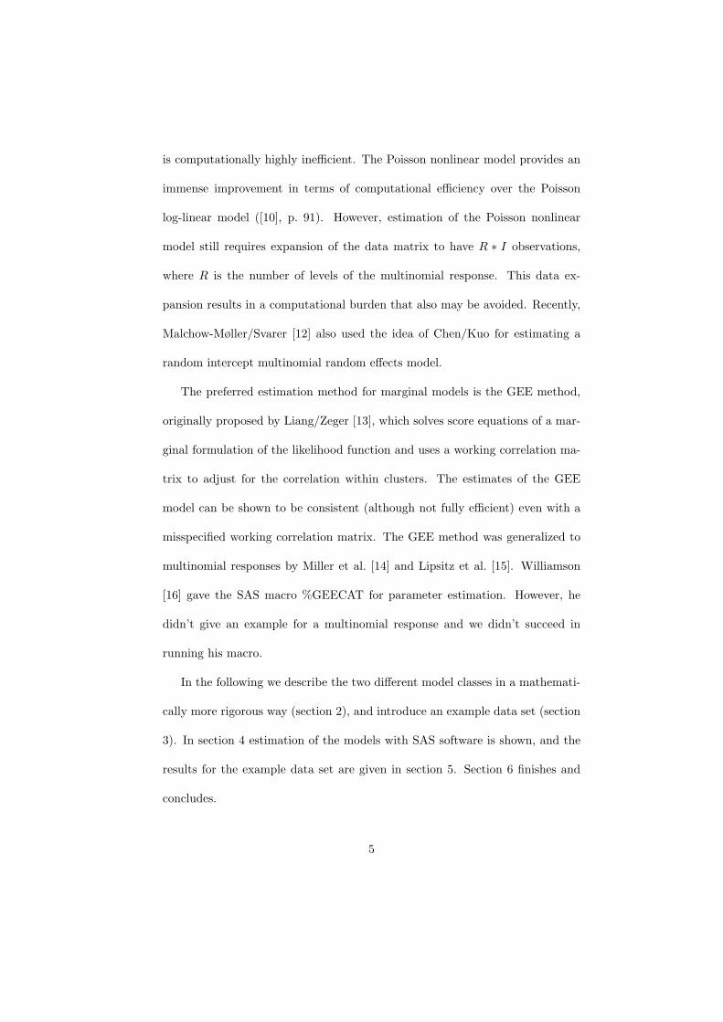
is computationally highly inefficient. The Poisson nonlinear model provides an

immense improvement in terms of computational efficiency over the Poisson

log-linear model ([10], p. 91). However, estimation of the Poisson nonlinear

model still requires expansion of the data matrix to have R ∗ I observations,

where R is the number of levels of the multinomial response. This data ex-

pansion results in a computational burden that also may be avoided. Recently,

Malchow-Møller/Svarer [12] also used the idea of Chen/Kuo for estimating a

random intercept multinomial random effects model.

The preferred estimation method for marginal models is the GEE method,

originally proposed by Liang/Zeger [13], which solves score equations of a mar-

ginal formulation of the likelihood function and uses a working correlation ma-

trix to adjust for the correlation within clusters. The estimates of the GEE

model can be shown to be consistent (although not fully efficient) even with a

misspecified working correlation matrix. The GEE method was generalized to

multinomial responses by Miller et al. [14] and Lipsitz et al. [15]. Williamson

[16] gave the SAS macro %GEECAT for parameter estimation. However, he

didn’t give an example for a multinomial response and we didn’t succeed in

running his macro.

In the following we describe the two different model classes in a mathemati-

cally more rigorous way (section 2), and introduce an example data set (section

3). In section 4 estimation of the models with SAS software is shown, and the

results for the example data set are given in section 5. Section 6 finishes and

concludes.

5

2 The Models

We assume that our data comprises a set of I (i = 1, . . . , I) independent clus-

ters where the i-th cluster consists of ni observations. Let Yij denote the j-

th response in cluster i (j = 1, . . . , ni), where this response is from one of r

(r = 1, . . . , R) distinct categories. Further, xij denotes a column vector of p

covariates for the j-th observation in the i-th cluster.

2.1 The random effects model

The model equation for a multinomial logistic model with random intercepts is

given by

log(

πijr

πij1

)= θr + x′ijβr + uir, r = 1, . . . , R (1)

where πijr = P (Yij = r) are response probabilities, the θr are constant terms

and the influences of covariates are assessed through the components of βr =

(β1r, . . . , βpr)′. The θr and the βr are considered to be fixed effects. For the ran-

dom intercepts uir we assume a multivariate normal distribution with zero ex-

pectation and unstructured covariance matrix Σ. That is, for ui = (ui1 . . . , uiR)′

we have ui ∼ N(0, Σ). For reasons of identification of parameters we restrict

θ1 = 0, β1 = 0, and u1 = 0, so that interpretation of parameters is with refer-

ence to the first category and Σ is actually a (R − 1) × (R − 1) matrix. The

likelihood contribution of the i-th cluster is

li(θr, βr, Σ) =∫ ∞

−∞

ni∏

j=1

[exp(θr + x′ijβr + uir)∑R

q=1 exp(θq + x′ijβq + uiq)

]I(Yij=r) fu(ui,Σ) dui

(2)

6

where fu(ui, Σ) is the multivariate normal density and I() the indicator function.

The overall likelihood function is the product of the contributions li from the

I clusters. Maximum likelihood estimation of the parameters is difficult due to

the fact that the likelihood function consists of a product of I integrals where

each of those cannot be solved in closed form. Thus, numerical or stochastic

integration are viable alternatives. Note that we restricted our attention to

multinomial models with random intercepts only. However, generalization to

models with random slope parameters is straightforward.

2.2 The marginal model

To specify a multinomial logistic model for correlated responses as a marginal

model we reorganise the response vector. We now write Yij as an ((R− 1)× 1)-

vector Y ∗ij of binary indicator variables Y ∗

ijr such that Yij = 2, . . . , R results in

Y ∗ij = 1 in column r and 0 anywhere else. In the case of Yij = 1 (reference cate-

gory), Y ∗ij = 0 in all R − 1 columns. This reorganisation of the response vector

can be interpreted as transforming the multinomial model into a multivariate

binary model. Hartzel et al. [1] use the term ’MGLMM’ (Multivariate General-

ized Linear Mixed Models) to describe these models. Let Y ∗i = (Y ∗′

i1 , . . . , Y ∗′ini

)′

denote the (ni(R− 1)× 1) response vector for the i-th cluster with expectation

π∗i and covariance matrix V ∗i . This covariance matrix V ∗

i is a ’double-block’

diagonal matrix where the (R−1)× (R−1)-block for (r, r′) on the ’inner’ block

of the main diagonal of V ∗i is a multinomial covariance matrix (see [11], Sect.

5.3.2) for the j-th observation in the i-th cluster and the remaining elements

7

on the ’outer’ block specify the covariance between two different observations

(j, j′) in the i-th cluster. Formally, this amounts to

V ∗i = cov(Y ∗

ijr, Y∗ij′r′) =

π∗ijr(1− π∗ijr) if j = j′, r = r′

−π∗ijrπ∗ijr′ if j = j′, r 6= r′

corr(Y ∗ijr,Y ∗ij′r′ )

[π∗ijr

(1−π∗ijr

)π∗ij′r′ (1−π∗

ij′r′ )]1/2 if j 6= j′

,

(3)

where the first two lines of (3) correspond to the ’inner’ block of V ∗i , the third

line to the ’outer’ block, and π∗ijr = E(Y ∗ijr = 1). It should be noted that the

third line does not constitute a circular definition. Instead, corr(Y ∗ijr, Y

∗ij′r′)

must be given a working correlation pattern in the analysis [14].

The model equation then is

log(

π∗ir1− π∗ir

)= θ∗r + x′ijβ

∗r , r = 2, . . . , R, (4)

where π∗ir denotes the expectation of all elements of Y ∗i belonging to response

category r. Note that there is no reference to a random effect in the model

equation.

Several choices are possible for the working form of the covariance matrix

V ∗i , ranging from the most simple assumption of independence within clusters

(corr(Y ∗ijr, Y

∗ij′r′) ≡ 0 if j 6= j′) to the most complex form, where all ((R−1)(R−

2)/2 ∗ ni(ni − 1)/2) parameters vary. Choosing V ∗i as closely as possible to the

true correlation matrix in general results in a gain of efficiency. However, O’Hara

Hines [17] and Lumley [18] note for the case of GEE estimation with ordinal

responses that careful modelling of the covariance structures is unnecessary and

in some cases even can be dangerous.

8

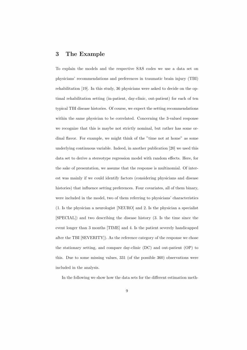
3 The Example

To explain the models and the respective SAS codes we use a data set on

physicians’ recommendations and preferences in traumatic brain injury (TBI)

rehabilitation [19]. In this study, 36 physicians were asked to decide on the op-

timal rehabilitation setting (in-patient, day-clinic, out-patient) for each of ten

typical TBI disease histories. Of course, we expect the setting recommendations

within the same physician to be correlated. Concerning the 3-valued response

we recognize that this is maybe not strictly nominal, but rather has some or-

dinal flavor. For example, we might think of the ”time not at home” as some

underlying continuous variable. Indeed, in another publication [20] we used this

data set to derive a stereotype regression model with random effects. Here, for

the sake of presentation, we assume that the response is multinomial. Of inter-

est was mainly if we could identify factors (considering physicians and disease

histories) that influence setting preferences. Four covariates, all of them binary,

were included in the model, two of them referring to physicians’ characteristics

(1. Is the physician a neurologist [NEURO] and 2. Is the physician a specialist

[SPECIAL]) and two describing the disease history (3. Is the time since the

event longer than 3 months [TIME] and 4. Is the patient severely handicapped

after the TBI [SEVERITY]). As the reference category of the response we chose

the stationary setting, and compare day-clinic (DC) and out-patient (OP) to

this. Due to some missing values, 331 (of the possible 360) observations were

included in the analysis.

In the following we show how the data sets for the different estimation meth-

9

ods should be set up in SAS.

The multinomial random effects model can be fitted to the data set tbisingle

which has one observation for each multinomial physician’s (physician) rec-

ommendation Yij (setting) and the four covariates neuro, special, time,

and severity. The response setting is coded as setting=1 for stationary,

setting=2 for day-clinic and setting=3 for out-patient rehabilitation settings.

DATA tbisingle;

INPUT physician setting neuro special time severity;

CARDS;

1 1 1 0 1 1

1 2 1 0 0 1

1 2 1 1 0 1

...

36 1 1 1 0 1

36 1 1 1 0 1

36 3 1 1 1 0

;

RUN;

The data set tbidouble which we employ to fit the marginal model is con-

structed with (R − 1) records for each observation in tbisingle. The r-th

observation Y ∗ijr, r = 1, 2 of tbidouble returned from each original observation

is coded 1 when Yij = r + 1 (as we employed Yij = 1 as the referent level). We

also construct an indicator NewIntercept of which response level is coded for

10

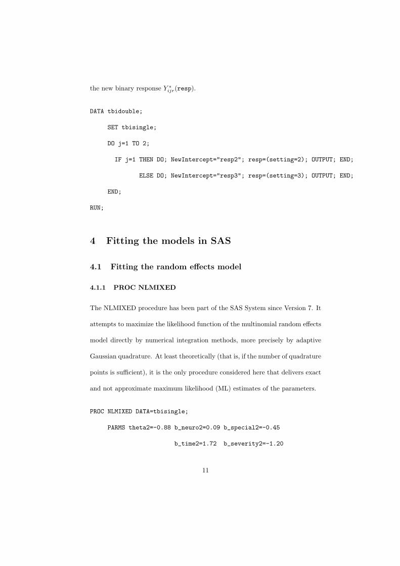
the new binary response Y ∗ijr(resp).

DATA tbidouble;

SET tbisingle;

DO j=1 TO 2;

IF j=1 THEN DO; NewIntercept="resp2"; resp=(setting=2); OUTPUT; END;

ELSE DO; NewIntercept="resp3"; resp=(setting=3); OUTPUT; END;

END;

RUN;

4 Fitting the models in SAS

4.1 Fitting the random effects model

4.1.1 PROC NLMIXED

The NLMIXED procedure has been part of the SAS System since Version 7. It

attempts to maximize the likelihood function of the multinomial random effects

model directly by numerical integration methods, more precisely by adaptive

Gaussian quadrature. At least theoretically (that is, if the number of quadrature

points is sufficient), it is the only procedure considered here that delivers exact

and not approximate maximum likelihood (ML) estimates of the parameters.

PROC NLMIXED DATA=tbisingle;

PARMS theta2=-0.88 b_neuro2=0.09 b_special2=-0.45

b_time2=1.72 b_severity2=-1.20

11

theta3=-2.43 b_neuro3=1.07 b_special3=0.30

b_time3=3.15 b_severity3=-2.02

logsu2=.5 logsu3=.5 z23=1;

eta1 = 0;

eta2 = theta2 + b_neuro2*neuro + b_special2*special +

b_time2*time + b_severity2*severity + u2;

eta3 = theta3 + b_neuro3*neuro + b_special3*special +

b_time3*time + b_severity3*severity + u3;

ARRAY exp_eta {3};

exp_eta1 = 1;

exp_eta2 = exp(eta2);

exp_eta3 = exp(eta3);

bot = exp_eta1 + exp_eta2 + exp_eta3;

p_setting = exp_eta{setting} / bot;

ll=log(p_setting);

su2 = exp(logsu2);

su3 = exp(logsu3);

rho23 = (exp(2*Z23) - 1) / (exp(2*Z23) + 1);

cov23 = rho23*su2*su3;

12

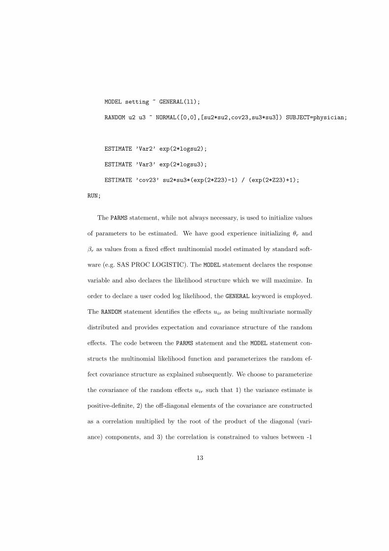
MODEL setting ~ GENERAL(ll);

RANDOM u2 u3 ~ NORMAL([0,0],[su2*su2,cov23,su3*su3]) SUBJECT=physician;

ESTIMATE ’Var2’ exp(2*logsu2);

ESTIMATE ’Var3’ exp(2*logsu3);

ESTIMATE ’cov23’ su2*su3*(exp(2*Z23)-1) / (exp(2*Z23)+1);

RUN;

The PARMS statement, while not always necessary, is used to initialize values

of parameters to be estimated. We have good experience initializing θr and

βr as values from a fixed effect multinomial model estimated by standard soft-

ware (e.g. SAS PROC LOGISTIC). The MODEL statement declares the response

variable and also declares the likelihood structure which we will maximize. In

order to declare a user coded log likelihood, the GENERAL keyword is employed.

The RANDOM statement identifies the effects uir as being multivariate normally

distributed and provides expectation and covariance structure of the random

effects. The code between the PARMS statement and the MODEL statement con-

structs the multinomial likelihood function and parameterizes the random ef-

fect covariance structure as explained subsequently. We choose to parameterize

the covariance of the random effects uir such that 1) the variance estimate is

positive-definite, 2) the off-diagonal elements of the covariance are constructed

as a correlation multiplied by the root of the product of the diagonal (vari-

ance) components, and 3) the correlation is constrained to values between -1

13

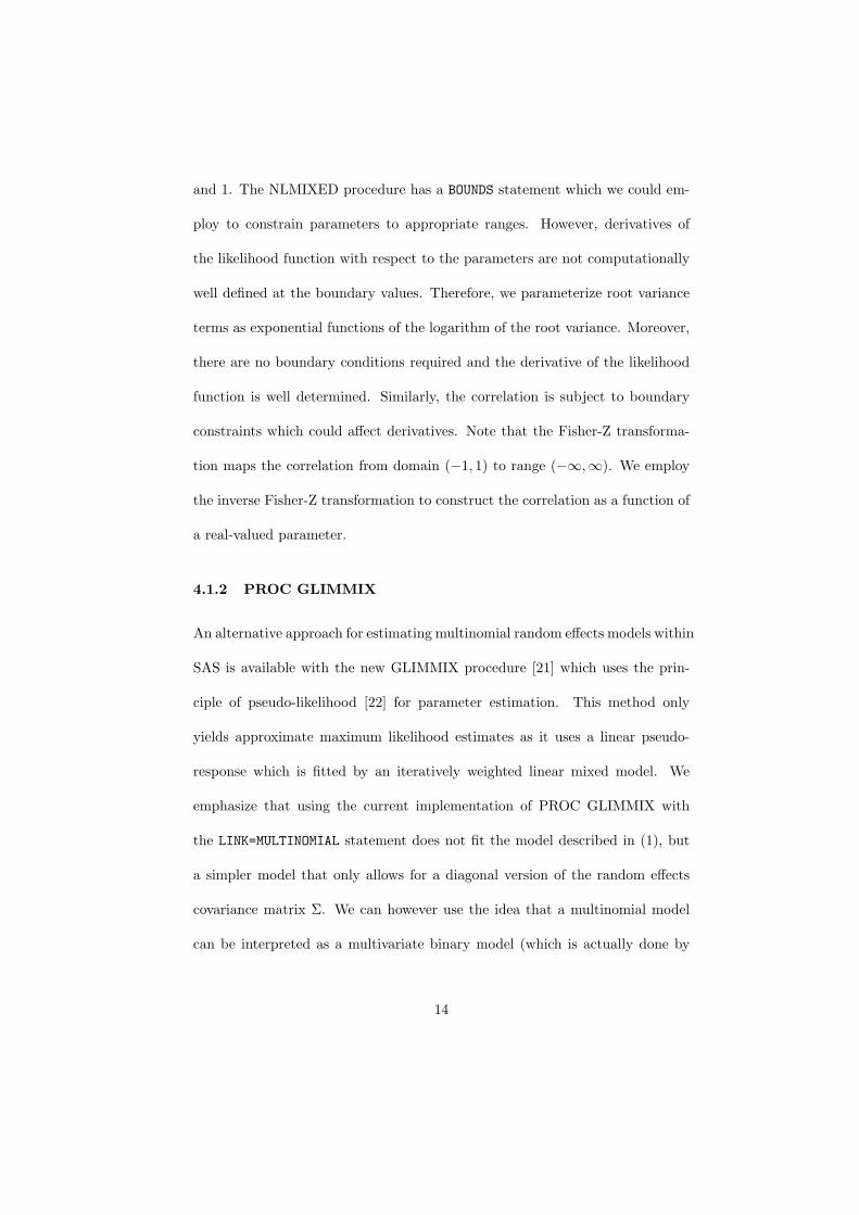
and 1. The NLMIXED procedure has a BOUNDS statement which we could em-

ploy to constrain parameters to appropriate ranges. However, derivatives of

the likelihood function with respect to the parameters are not computationally

well defined at the boundary values. Therefore, we parameterize root variance

terms as exponential functions of the logarithm of the root variance. Moreover,

there are no boundary conditions required and the derivative of the likelihood

function is well determined. Similarly, the correlation is subject to boundary

constraints which could affect derivatives. Note that the Fisher-Z transforma-

tion maps the correlation from domain (−1, 1) to range (−∞,∞). We employ

the inverse Fisher-Z transformation to construct the correlation as a function of

a real-valued parameter.

4.1.2 PROC GLIMMIX

An alternative approach for estimating multinomial random effects models within

SAS is available with the new GLIMMIX procedure [21] which uses the prin-

ciple of pseudo-likelihood [22] for parameter estimation. This method only

yields approximate maximum likelihood estimates as it uses a linear pseudo-

response which is fitted by an iteratively weighted linear mixed model. We

emphasize that using the current implementation of PROC GLIMMIX with

the LINK=MULTINOMIAL statement does not fit the model described in (1), but

a simpler model that only allows for a diagonal version of the random effects

covariance matrix Σ. We can however use the idea that a multinomial model

can be interpreted as a multivariate binary model (which is actually done by

14

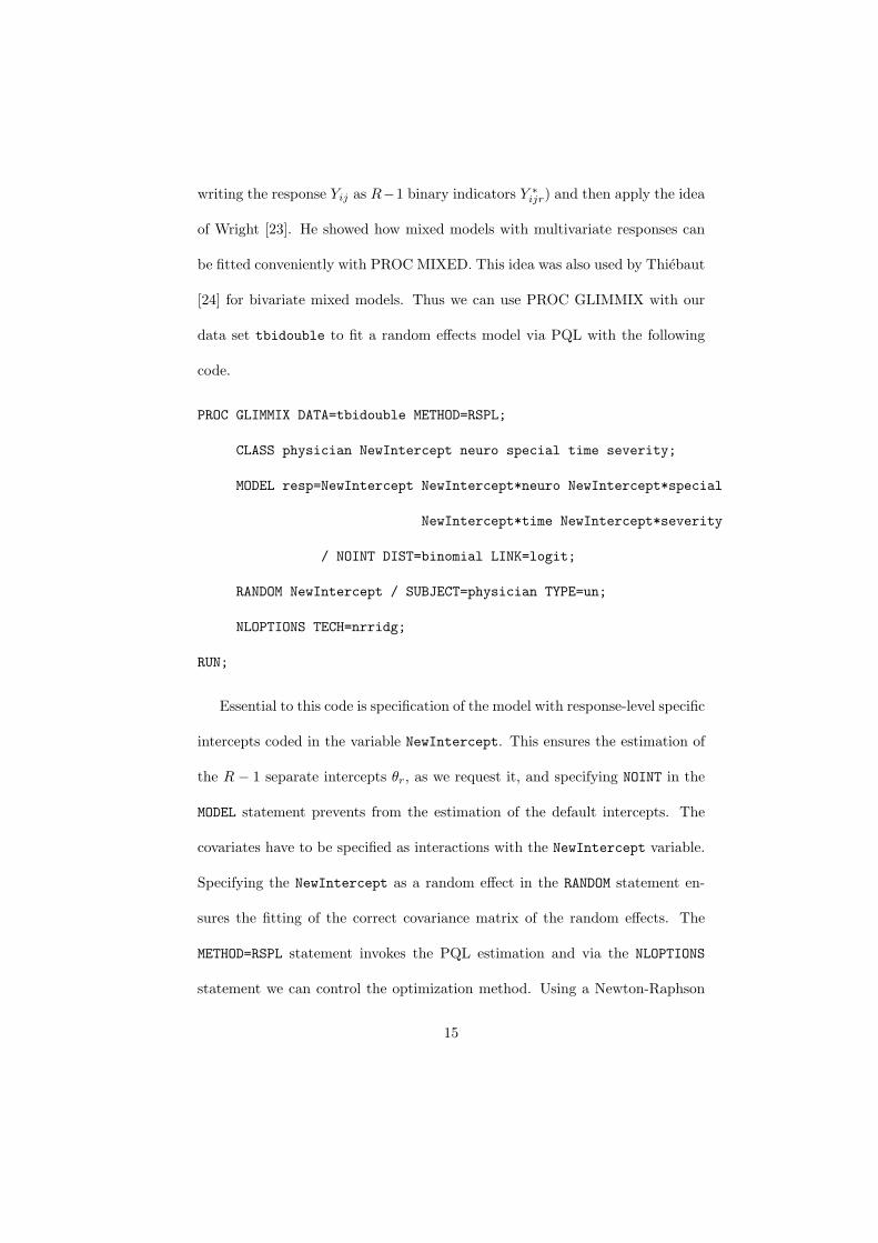
writing the response Yij as R−1 binary indicators Y ∗ijr) and then apply the idea

of Wright [23]. He showed how mixed models with multivariate responses can

be fitted conveniently with PROC MIXED. This idea was also used by Thiebaut

[24] for bivariate mixed models. Thus we can use PROC GLIMMIX with our

data set tbidouble to fit a random effects model via PQL with the following

code.

PROC GLIMMIX DATA=tbidouble METHOD=RSPL;

CLASS physician NewIntercept neuro special time severity;

MODEL resp=NewIntercept NewIntercept*neuro NewIntercept*special

NewIntercept*time NewIntercept*severity

/ NOINT DIST=binomial LINK=logit;

RANDOM NewIntercept / SUBJECT=physician TYPE=un;

NLOPTIONS TECH=nrridg;

RUN;

Essential to this code is specification of the model with response-level specific

intercepts coded in the variable NewIntercept. This ensures the estimation of

the R − 1 separate intercepts θr, as we request it, and specifying NOINT in the

MODEL statement prevents from the estimation of the default intercepts. The

covariates have to be specified as interactions with the NewIntercept variable.

Specifying the NewIntercept as a random effect in the RANDOM statement en-

sures the fitting of the correct covariance matrix of the random effects. The

METHOD=RSPL statement invokes the PQL estimation and via the NLOPTIONS

statement we can control the optimization method. Using a Newton-Raphson

15

technique with ridging (TECH=nrridg) proved to be very efficient.

4.2 Fitting the marginal effects model

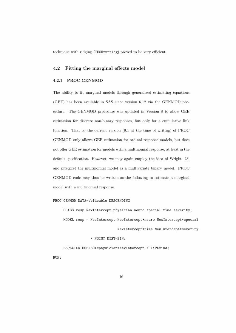
4.2.1 PROC GENMOD

The ability to fit marginal models through generalized estimating equations

(GEE) has been available in SAS since version 6.12 via the GENMOD pro-

cedure. The GENMOD procedure was updated in Version 8 to allow GEE

estimation for discrete non-binary responses, but only for a cumulative link

function. That is, the current version (9.1 at the time of writing) of PROC

GENMOD only allows GEE estimation for ordinal response models, but does

not offer GEE estimation for models with a multinomial response, at least in the

default specification. However, we may again employ the idea of Wright [23]

and interpret the multinomial model as a multivariate binary model. PROC

GENMOD code may thus be written as the following to estimate a marginal

model with a multinomial response.

PROC GENMOD DATA=tbidouble DESCENDING;

CLASS resp NewIntercept physician neuro special time severity;

MODEL resp = NewIntercept NewIntercept*neuro NewIntercept*special

NewIntercept*time NewIntercept*severity

/ NOINT DIST=BIN;

REPEATED SUBJECT=physician*NewIntercept / TYPE=ind;

RUN;

16

This code parallels the previous PROC GLIMMIX for the random effects

model in most relevant aspects. However, instead of using the RANDOM state-

ment to model the correlation of responses within subjects, we now have to

use the REPEATED statement. The subject effect is specified as an interaction of

the intercept indicator NewIntercept with the original subject variable. Un-

fortunately, the current implementation of PROC GENMOD only allows the

specification of an independent working correlation matrix TYPE=ind for the

case with interacting subject effects. This results in a working correlation ma-

trix that is a complete identity matrix (elements in the two last rows of (3) are

identically 0), and contradicts the idea of a multinomial covariance matrix for

the ’inner’ block.

4.2.2 PROC GLIMMIX

A partial solution to the problem of an a priori misspecified working correlation

matrix in PROC GENMOD is to use a different but closely connected estimation

method for marginal models, the so called marginal quasi-likelihood (MQL)

estimator [25]. This is actually an estimation method for the random effects

model, but it was shown [25] that this approach has an identical estimating

equation for the first moment as the standard GEE approach of Liang/Zeger [13].

However, it uses a more efficient estimating equation for the second moments

(see [26], p. 163f.). Thus, we expect similar estimates in real data applications.

MQL estimation can be realized within SAS by using PROC GLIMMIX with

the METHOD=MMPL option for parameter estimation.

17

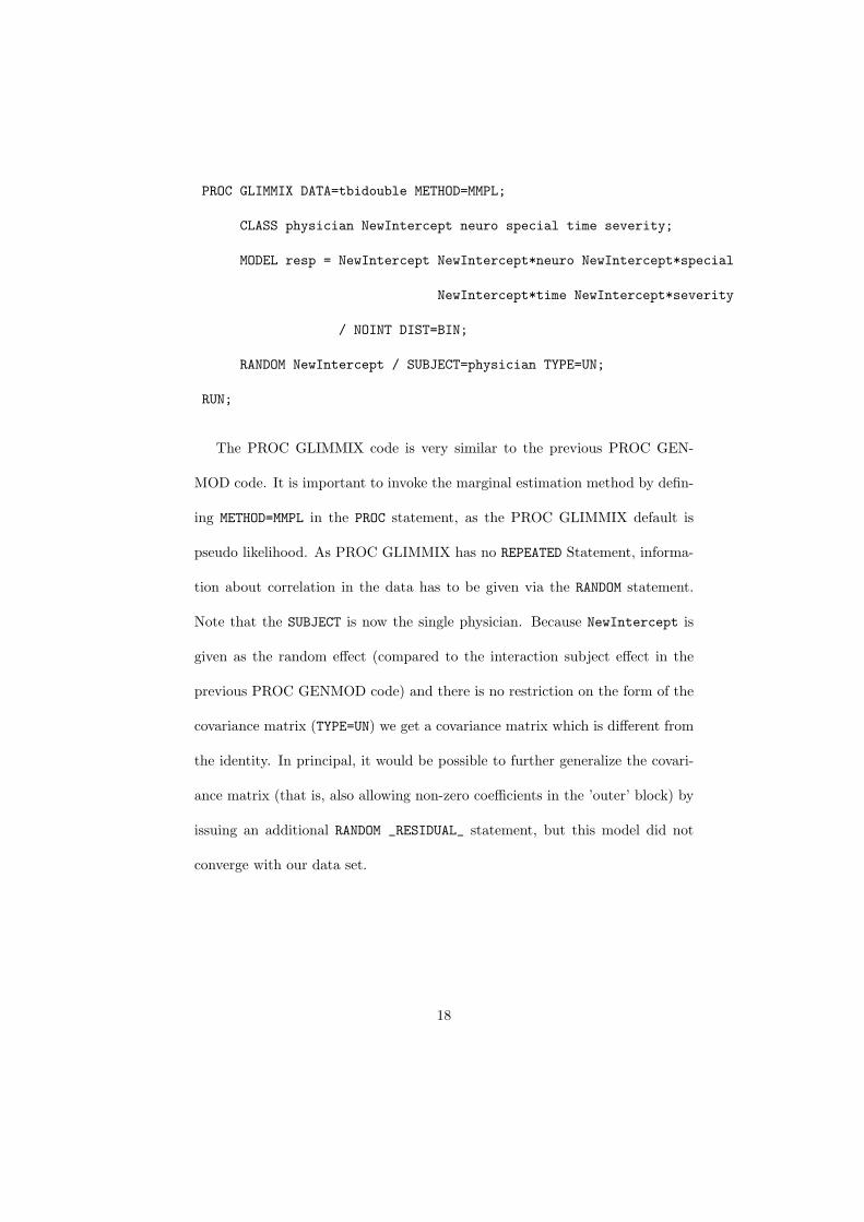
PROC GLIMMIX DATA=tbidouble METHOD=MMPL;

CLASS physician NewIntercept neuro special time severity;

MODEL resp = NewIntercept NewIntercept*neuro NewIntercept*special

NewIntercept*time NewIntercept*severity

/ NOINT DIST=BIN;

RANDOM NewIntercept / SUBJECT=physician TYPE=UN;

RUN;

The PROC GLIMMIX code is very similar to the previous PROC GEN-

MOD code. It is important to invoke the marginal estimation method by defin-

ing METHOD=MMPL in the PROC statement, as the PROC GLIMMIX default is

pseudo likelihood. As PROC GLIMMIX has no REPEATED Statement, informa-

tion about correlation in the data has to be given via the RANDOM statement.

Note that the SUBJECT is now the single physician. Because NewIntercept is

given as the random effect (compared to the interaction subject effect in the

previous PROC GENMOD code) and there is no restriction on the form of the

covariance matrix (TYPE=UN) we get a covariance matrix which is different from

the identity. In principal, it would be possible to further generalize the covari-

ance matrix (that is, also allowing non-zero coefficients in the ’outer’ block) by

issuing an additional RANDOM _RESIDUAL_ statement, but this model did not

converge with our data set.

18

5 Results

Table 1 provides parameter estimates and standard errors for our TBI data set

for the described models and estimation methods.

*** PLACE TABLE1 APPROXIMATELY HERE ***

Some remarks regarding the results can be made: As we expect (and maybe

hope as potential patients), physician characteristics (NEURO and SPECIAL)

have only small influence on their recommendations, estimates are rarely larger

than the corresponding standard errors. This is different for patient character-

istics. In all models we find positive and significant parameter estimates for

the TIME covariate, and this is true for the day-clinic (DC) as well as for the

out-patient (OP) category. That is, if the TBI occurred more than three months

ago, the physicians recommend the DC setting, and even stronger the OP set-

ting. Estimates for the SEVERITY covariate, on the contrary, are negative in

all models, that is, if the TBI patients are severely handicapped after the in-

cident, the physicians recommend more frequently the stationary setting. The

OP setting has larger negative estimates compared to the DC setting, which

means that the OP setting is the least recommended in severely handicapped

patients. As a rough summary, with more severe TBI and shorter time since

TBI, physicians are more likely to recommend stationary rehabilitation.

Comparing the various estimation methods, we find that GEE and MQL

estimates are very similar. This can be explained by the fact that MQL es-

timation is only a slightly improved GEE estimation. In contrast, estimates

from the two RE estimation methods (GQ and PQL) differ - sometimes sub-

19

stantially. This is most likely due to differences in estimation of the variance

components. It is well known that the PQL method underestimates the random

effects variances [27]. As expected, random effect variance estimates are largest

for Gaussian quadrature. Shrinkage of the variance component estimates has

led to heavy criticism of MQL and PQL methods and several proposals for their

improvement. We observe that the within-physician covariance for DC and OP

settings is positive only for the GQ results. If we were to regard the different

treatments for TBI as ordinal, then we would expect physician willingness for

a less controlled treatment environment to be positively correlated. That is, a

physician who is more likely to recommend a day-clinic treatment plan for a

patient who has had some time to recover from a moderately severe TBI would

also be more likely to recommend an out-patient treatment plan for a patient

who has had a less severe TBI or more time to recover.

There is, apparently, considerable between-physician variability (or, equiva-

lently, within-physician correlation) in rehabilitation setting recommendations.

Model likelihood can be obtained from both the fixed effect and random effect

model, allowing a likelihood ratio test for the contribution of the random effects.

With 3 df , the difference in −2LL of 31.7 is significant at p < 0.001.

6 Discussion

We have shown four different methods in SAS to estimate multinomial regres-

sion models for correlated responses. All methods proved to be very stable in

20

view of the complexity of the estimation process and the small data set. We like

to emphasize again that the current (Version 9.1 at the time of writing) imple-

mentations of PROC GENMOD and PROC GLIMMIX do not allow a direct

estimation of multinomial logistic regression with correlated responses. This is

only possible after reorganising the data and using the idea of Wright [23].

The main motivation for this paper was to caution against the idea of

Chen/Kuo [10] and Malchow-Møller/Svarer [12] to use the ’Poisson-trick’ for

the estimation of the random effects models. The two proposed Poisson models

of Chen/Kuo [10] are computationally inefficient as they use a larger than nec-

essary number of parameters (in the case of the Poisson log-linear model) or a

larger than necessary data set (in the case of the Poisson nonlinear model) to

set up the models.

To demonstrate the inefficiency of the Poisson models we compared com-

puting time between the different procedures for our data set. Our NLMIXED

code (from section 4.1.1) required 16 seconds to converge on an IBM desktop PC

(Pentium 4, 3 GHz, 2 GB RAM). The Poisson nonlinear model of Chen/Kuo [10]

took 5 Minutes 20 seconds to converge, computing time thus being enlarged to

the 20-fold. However, and as expected, parameter estimates and their standard

errors were identical for the two models.

Code for the Poisson nonlinear model is provided in an appendix so that the

reader may compare results for the different estimation methods in his/her own

computing environment or with his/her own data sets. It is obvious that the

achieved computational efficiency with our NLMIXED code is not paid for by

21

an increased programming time, the code for the Poisson nonlinear model dif-

fers only in some minor aspects. It is also worth noting that the log-likelihood

value for the Poisson nonlinear model is deflated by the number of observa-

tions employed. Employing the multinomial distribution returns the correct

log-likelihood.

The Poisson log-linear model also converged with our data but yielded only

nonsense results which is not unexpected as 349 parameters are estimated.

7 Acknowledgement

This work has been sponsored in part by the Bundesministerium fur Bildung und

Forschung (BMBF), Wilhelm-Roux-Programm zur Nachwuchs- und Forschungs-

forderung der Medizinischen Fakultat der Martin-Luther-Universitat Halle-Wit-

tenberg (Anschubantrag, FKZ: 5/08). We are grateful to Oliver Schabenberger

from SAS Institute who helped us to understand the new GLIMMIX procedure.

8 Appendix

As previously described, the data have to be reorganised for fitting the Poisson

nonlinear model. This reorganisation is very much like the one which is employed

for the marginal model with the difference that we have to build R records for

each observation in tbisingle.

DATA tbiPoisson;

SET tbisingle;

22

ARRAY resp {3};

DO level=1 to 3;

response = (resp{level}=1);

OUTPUT;

END;

RUN;

The NLMIXED code for parameter estimation is very similar to the one

used for the multinomial likelihood model in 4.1.1. The main difference is the

use of the Poisson likelihood in the MODEL statement. To be concrete, in our

NLMIXED code in 4.1.1 the line

• PROC NLMIXED DATA=tbisingle;

should be replaced by

PROC NLMIXED DATA=tbiPoisson;

• p_setting = exp_eta{setting} / bot;

ll=log(p_setting);

should be replaced by

lambda=exp_eta{level} / bot;

• MODEL setting ~ GENERAL(ll);

should be replaced by

MODEL response ~ POISSON(lambda);

23

References

[1] J. Hartzel, A. Agresti, B. Caffo, Multinomial Logit Random Effects Models,

Statistical Modelling 1 (2001) 81-102.

[2] D. Revelt, K. Train, Mixed Logit with Repeated Choices: Households’

Choices of Appliance Efficiency Level, The Review of Economics and Sta-

tistics 80 (1998) 647-657.

[3] D. Hedeker, A mixed-effects multinomial logistic regression model, Statis-

tics in Medicine 22 (2003) 1433-46.

[4] A. Skrondal, S. Rabe-Hesketh, Multilevel logistic regression for polytomous

data and rankings, Psychometrika 68 (2003) 267-287.

[5] M.J. Daniels, C. Gatsonis, Hierarchical polytomous regression models with

applications to health services research, Statistics in Medicine 16 (1997)

2311-2325.

[6] P.J. Diggle, K.Y. Liang, S.L. Zeger, Analysis of Longitudinal Data, Oxford

University Press, Oxford, 1994.

[7] D. Brownstone, K. Train, Forecasting New Product Penetration With Flex-

ible Substitution Patterns, Journal of Econometrics 89 (1998) 109-129.

[8] K. Train, http://elsa.berkeley.edu/ train/software.html, 2007.

[9] D. Hedeker, MIXNO: A computer program for mixed-effects nominal logis-

tic regression. Journal of Statistical Software 80 (1998) 647-657.

24

[10] Z. Chen, L. Kuo, A Note on the Estimation of the Multinomial Logit Model

With Random Effects, The American Statistician 55 (2000) 89-95.

[11] P. McCullagh, J.A. Nelder, Generalized Linear Models, Chapman & Hall,

London, 1989.

[12] N. Malchow-Møller, M. Svarer, Estimation of the Multinomial Logit Model

with Random Effects, Applied Economics Letters 10 (2003) 389-392.

[13] K.Y. Liang, S.L. Zeger, Longitudinal Data Analysis Using Generalized Lin-

ear Models, Biometrika 73 (1986) 13-22.

[14] M.E. Miller, C.C. Davis, J.R. Landis, The analysis of longitudinal poly-

tomous data: Generalized estimating equations and connections with

weighted least squares, Biometrics 49 (1993) 1033-1044.

[15] S.R. Lipsitz, K. Kim, L. Zhao, Analysis of repeated categorical data using

generalized estimating equations, Statistics in Medicine 13 (1994) 1149-

1163.

[16] J.M. Williamson, S.R. Lipsitz, K.M. Kim, GEECAT and GEEGOR: com-

puter programs for the analysis of correlated categorical response data,

Computer Methods and Programs in Biomedicine 58 (1999) 25-34.

[17] R.J. O’Hara Hines, Analysis of Clustered Polytomous Data Using General-

ized Estimating Equations and Working Covariance Structures, Biometrics

53 (1997) 1552-1556.

25

[18] T. Lumley, Generalized Estimating Equations for Ordinal Data: A Note

on Working Correlation Structures and Working Covariance Structures,

Biometrics 52 (1996) 354-361.

[19] U. Hasenbein, O. Kuss, M. Baumer, C. Schert, H. Schneider, C.W.

Wallesch, Physicians’ preferences and expectations in traumatic brain in-

jury rehabilitation - results of a case-based questionnaire survey, Disability

and Rehabilitation 25 (2003) 136-142.

[20] O. Kuss, Modelling Physicians’ Recommendations for Optimal Medical

Care by Random Effects Stereotype Regression, in Proceedings of the

18th International Workshop on Statistical Modelling, eds. G. Verbeke, G.

Molenberghs, M. Aerts, S. Fieuws, pp. 245-249. (Katholieke Universiteit

Leuven, Leuven, 2003).

[21] O. Schabenberger, Introducing the GLIMMIX Procedure for Generalized

Linear Mixed Models. Proceedings of the 30th Annual SAS Users Group

International (SUGI) Conference (2005) Paper 196-30.

[22] R. Wolfinger, M. O’Connell, Generalized Linear Mixed Models: a Pseudo-

Likelihood Approach, Journal of Statistical and Computational Simulation

48 (1993) 233243.

[23] S.P. Wright, Multivariate Analysis Using the MIXED Procedure, Proceed-

ings of the 23th Annual SAS Users Group (SUGI) International Conference

(1998) Paper 229-23.

26

[24] R. Thiebaut, H. Jacqmin-Gadda, G. Chene, C. Leport, D. Commenges,

Bivariate linear mixed models using SAS proc MIXED, Computer Methods

and Programs in Biomedicine 69 (2002) 249-256.

[25] N.E. Breslow, D.G. Clayton, Approximate Inference in Generalized Linear

Mixed Models, Journal of the American Statistical Association 88 (1993)

925.

[26] M. Davidian, D.M. Giltinan, Nonlinear Models for Repeated Measurement

Data, Chapman & Hall, London, 1995.

[27] G. Rodriguez, N. Goldman, An Assessment of Estimation Procedures for

Multilevel Models with Binary Responses, Journal of the Royal Statistical

Society, Series A 158 (1995) 73-89.

27

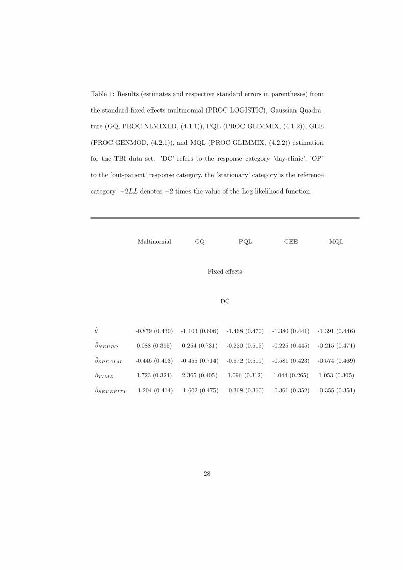
Table 1: Results (estimates and respective standard errors in parentheses) from

the standard fixed effects multinomial (PROC LOGISTIC), Gaussian Quadra-

ture (GQ, PROC NLMIXED, (4.1.1)), PQL (PROC GLIMMIX, (4.1.2)), GEE

(PROC GENMOD, (4.2.1)), and MQL (PROC GLIMMIX, (4.2.2)) estimation

for the TBI data set. ’DC’ refers to the response category ’day-clinic’, ’OP’

to the ’out-patient’ response category, the ’stationary’ category is the reference

category. −2LL denotes −2 times the value of the Log-likelihood function.

Multinomial GQ PQL GEE MQL

Fixed effects

DC

θ -0.879 (0.430) -1.103 (0.606) -1.468 (0.470) -1.380 (0.441) -1.391 (0.446)

βNEURO 0.088 (0.395) 0.254 (0.731) -0.220 (0.515) -0.225 (0.445) -0.215 (0.471)

βSPECIAL -0.446 (0.403) -0.455 (0.714) -0.572 (0.511) -0.581 (0.423) -0.574 (0.469)

βTIME 1.723 (0.324) 2.365 (0.405) 1.096 (0.312) 1.044 (0.265) 1.053 (0.305)

βSEV ERITY -1.204 (0.414) -1.602 (0.475) -0.368 (0.360) -0.361 (0.352) -0.355 (0.351)

28

OP

θ -2.429 (0.566) -3.009 (0.820) -3.267 (0.643) -3.034 (0.628) -3.046 (0.595)

βNEURO 1.073 (0.481) 1.329 (0.916) 1.085 (0.658) 1.054 (0.416) 1.050 (0.591)

βSPECIAL 0.296 (0.426) 0.281 (0.855) 0.447 (0.607) 0.466 (0.458) 0.435 (0.540)

βTIME 3.149 (0.456) 4.138 (0.588) 2.929 (0.469) 2.654 (0.483) 2.665 (0.441)

βSEV ERITY -2.022 (0.441) -2.591 (0.531) -1.589 (0.395) -1.485 (0.371) -1.470 (0.381)

Random effects

σ2DC – 1.650 (0.804) 0.590 (0.336) – 0.436 (0.273)

σ2OP – 2.611 (1.200) 1.032 (0.521) – 0.715 (0.369)

σ2DCOP – 1.888 (0.856) -0.119 (0.324) – -0.131 (0.244)

−2LL 492.9 461.2 – – –

No. ofparam. 10 13 – – –

29