A Novel Approach to Characterizing LiDAR Waveforms

Geoffrey M. HenebryEric Ariel L. SalasGeographic Information Science Center of ExcellenceSouth Dakota State University

and

Naikoa Aguilar-AmuchasteguiDepartment of Environmental StudiesUniversity of North Carolina-Wilmington[Forest Carbon Lead Scientist, World Wildlife Fund, as of 8/2010]

Research supported through the NASA Biodiversity program: NNX09AK23G. Thank you!

0

20

40

60

80

100

120

140

160

180

200

150 200 250 300 350

Pow

er

Waveform Location

La Selva Sample (275.98, 10.42)

1998

2005

Synergistic Analyses of Data from Active and Passive Sensors toAssess Relationships between Spatial Heterogeneity of TropicalForest Structure and Biodiversity Dynamics

Study site: Tropical forests on the Atlantic slope of Costa Rica, specifically, the stands under sustainable management by FUNDECOR, a Costa Rican NGO.

Project proposed: 6/2008Project funding received: 7/2009First field campaign: 6/2010

Focus today on a new approach that we very recently developed for characterizing LiDAR waveform data.

The Challenge of Analyzing LiDAR Waveforms - 1

LiDAR (Light Detection And Ranging) is an active remote sensing technology that

1.Uses laser light to illuminate the target area,2.Senses backscattering of the illuminating radiation, and3.Measures the time a laser pulse takes to travel back from regions of strong backscattering.

A LiDAR waveform sensor records the power of the backscattering signal at fine temporal resolution which can be converted to distance.

Thus, the term laser altimetry; LiDAR measures altitudes.

The Challenge of Analyzing LiDAR Waveforms - 2

But we are more interested in knowing elevations:

Terrain elevationabove or below the waterline

Vegetation height the crown of a specific tree or the nominal height of a canopy

Vertical profile through a multilayered canopy

resolving foliage densities to characterize habitat structure

The mapping from altitudes to elevations is complicated by many confounding factors.

0

20

40

60

80

100

120

140

160

180

200

150 200 250 300 350

Pow

er

Waveform Location

La Selva Sample (275.98, 10.42)

1998

2005

The Challenge of Analyzing LiDAR Waveforms - 3

Waveform data have been actively collected for more than 15 years.

Analyses of detected waveforms have been approached in three ways:

1.Multiple Gaussian curves fit to approximate the waveform;

2.Metrics relating the backscattering power to the cumulative distribution of backscattered illumination, such as HOME (height of median energy); and

3.Descriptive statistics on the waveform.I contend there is a richness in LiDAR waveforms that has yet to be exploited by conventional analyses.

EXAMPLE 1:

Duncanson LI, Neimann KO, Wulder MA. 2010. Estimating forest canopy height and terrain relief from GLAS waveform metrics. Remote Sensing of Environment 114:138-154.

EXAMPLE 2:

Falkowski J. Evans JS, Martinuzzi S, Gessler PE, Hudak AT. 2009. Characterizing forest succession with lidar data: an evaluation for the inland Northwest, USA. Remote Sensing of Environment 113:946-056.

EXAMPLE 3:

Nelson R, Ranson KJ, Sun G, Kimes DS, Kharuk V, Montesano P. 2009. Estimating Siberian timber volume using MODIS and ICESat/GLAS. Remote Sensing of Environment 113: 691-701.

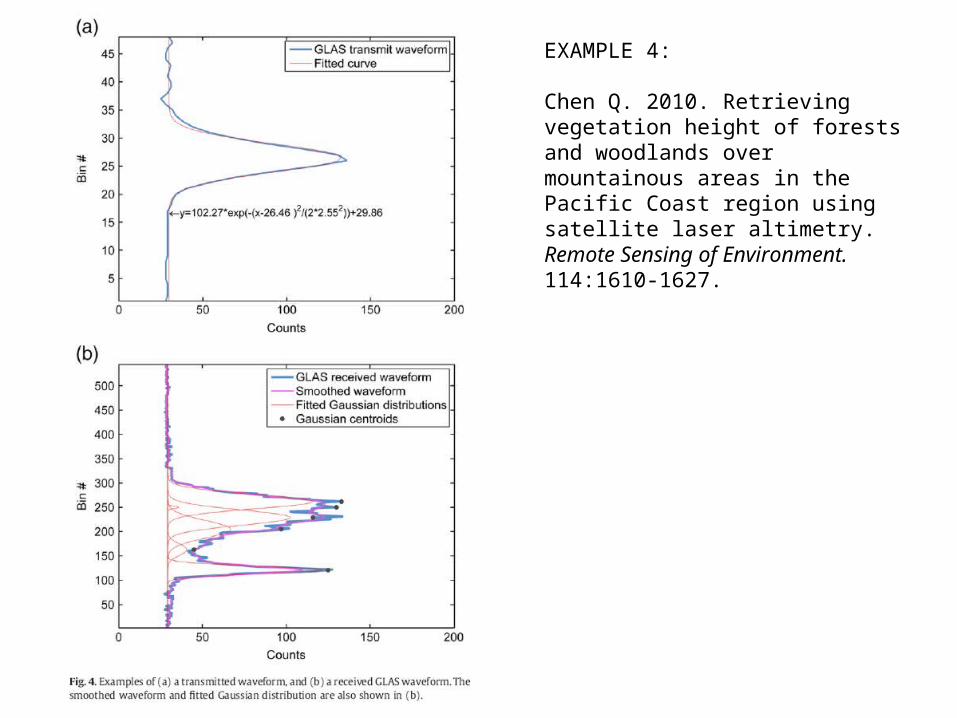
EXAMPLE 4:

Chen Q. 2010. Retrieving vegetation height of forests and woodlands over mountainous areas in the Pacific Coast region using satellite laser altimetry. Remote Sensing of Environment. 114:1610-1627.

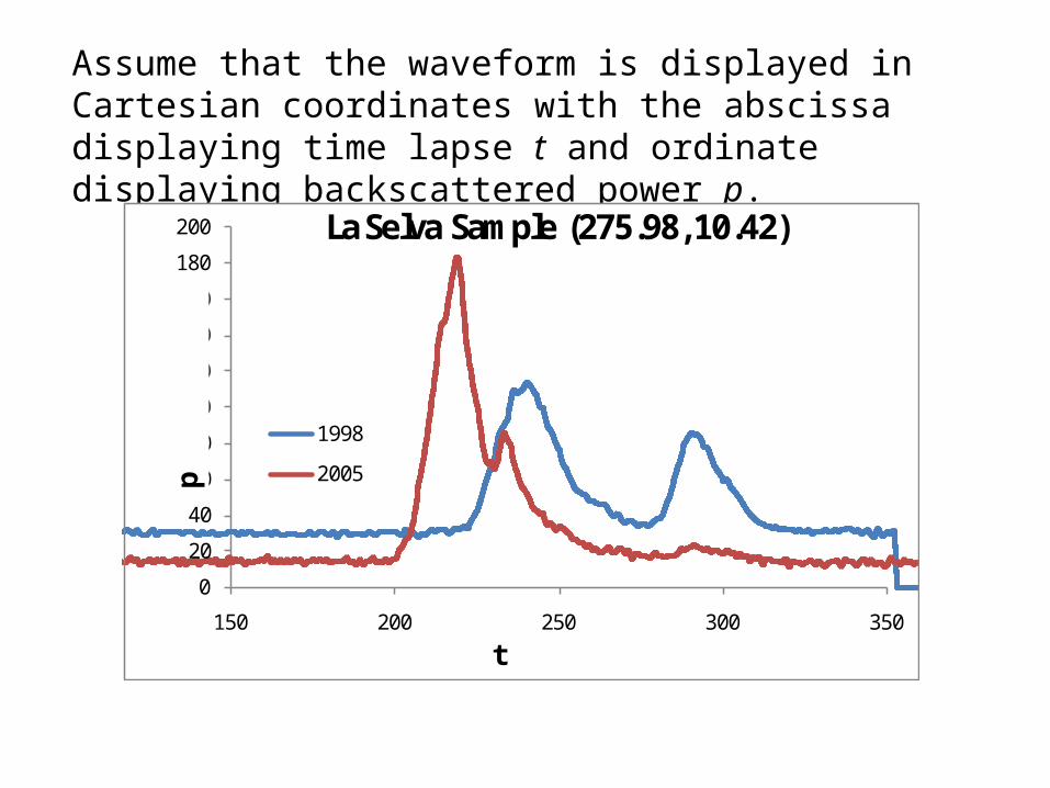
Assume that the waveform is displayed in Cartesian coordinates with the abscissa displaying time lapse t and ordinate displaying backscattered power p.

0

20

40

60

80

100

120

140

160

180

200

150 200 250 300 350

Pow

er

Waveform Location

La Selva Sample (275.98, 10.42)

1998

2005

t

p

0

20

40

60

80

100

120

140

150 200 250 300 350

Pow

er

Waveform Location (Time)

1998

P

Selected Pivots

Left Pivot Right Pivot

MDLP to 1st Max. PowerMDLP to DipMDLP to 2nd Max. Power

MD can be computed from RP.

MDLP to RP

MD can be computed from LP to any point on the curve. More points give better shape definition.

MDRP to 2nd Max. PowerMDRP to DipMDRP to 1st Max. PowerMDRP to LP

Moment Distance Method - 1Let the subscript LP denote the left pivot or earlier temporal reference point and subscript RP denote the right pivot or later temporal reference point.

t

Moment Distance Method - 2The MD framework is described in the following pair of equations:

The moment distance from the left pivot (MDLP) is the sum of the hypotenuses constructed from the left pivot to the power at successively later times (index i from tLP to tRP): one base of each triangle is the difference from the left pivot (i – tLP) along the abscissa and the other base is simply the power at i.

Similarly, the moment distance from the right pivot (MDRP) is the sum of the hypotenuses constructed from the right pivot to the power at successively earlier times (index i from tRP to tLP): one base of each triangle is the difference from the right pivot (tRP – i) along the abscissa and the other base is simply the power at i.

[1]

[2]

• In the 1998 La Selva waveform, there are 133 points on the curve between the LP and RP and the MDI = 749.93

• In the 2005 La Selva waveform, there are 153 points on the curve between the LP and RP and the MDI = 1538.18

Moment Distance Method - 3From this pair of moment distances, we form the Moment Distance Index (MDI) and the MDI Normalized (MDIN):

MDI = MDLP – MDRP [3]

MDIN = MDI / (MDLP + MDRP) [4]

We propose that MDI can be used to capture dynamics in canopy structure.

0

20

40

60

80

100

120

140

160

0 100 200 300 400 500

pow

er

bins

Figure 1b: Max Peak Late

0

20

40

60

80

100

120

140

160

0 100 200 300 400 500

pow

er

bins

Figure 1a: Max Peak Early

0

20

40

60

80

100

120

140

160

0 100 200 300 400 500

pow

er

bins

Figure 1c: Equal Peaks

Three waveform types found in LVIS data from La Selva

Max Peak Early

Max Peak Late

Equal Peaks

MDI vs. waveform landmarks

-200

-100

0

100

200

300

400

0 20 40 60 80 100

MD

I

Power of Early Max Peak

Figure 2bMax Peak Early

Equal Peaks

Max Peak Late

-200

-100

0

100

200

300

400

230 240 250 260 270 280

MD

I

Early Max Peak Bin Location

Figure 2aMax Peak Early

Equal Peaks

Max Peak Late

-200

-100

0

100

200

300

400

0 50 100 150 200

MD

I

Power of Late Max Peak

Figure 2c

Max Peak Early

Equal Peaks

Max Peak Late

Location of early max peak

Power of early max peak

Power of late max peak

0

40

80

120

160

-800

-600

-400

-200

0

200

0 20 40 60 80 100 120

Sim

ulat

ed W

ave

Retu

rn

MD

I

Time (years)

Figure 6b: first 120 years

MDI

First Peak

Mid Peak

Last Peak

0

40

80

120

160

-800

-600

-400

-200

0

200

0 100 200 300 400 500

Sim

ulat

ed W

ave

Retu

rn

MD

I

Time (years)

Figure 6a: 500 years

MDI

First Peak

Mid Peak

Last Peak

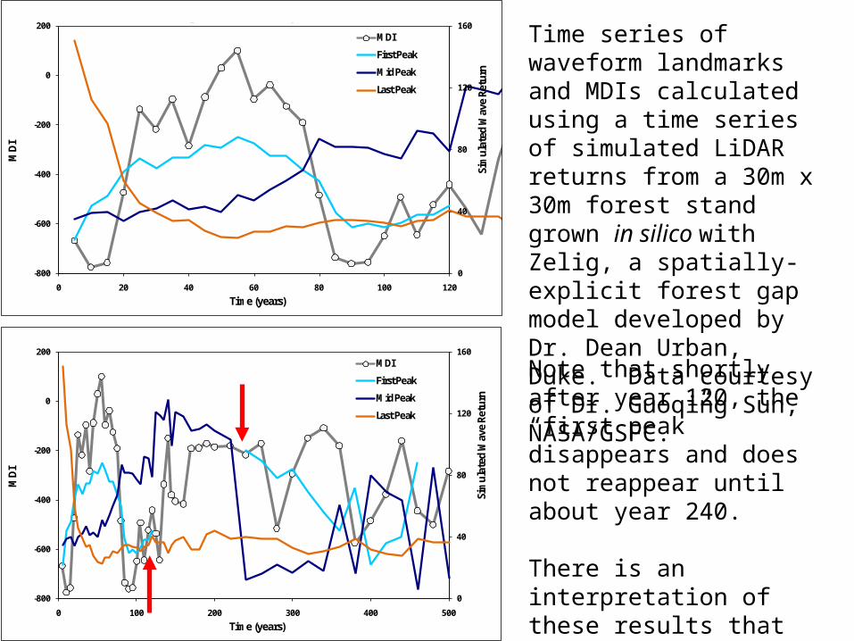
Time series of waveform landmarks and MDIs calculated using a time series of simulated LiDAR returns from a 30m x 30m forest stand grown in silico with Zelig, a spatially-explicit forest gap model developed by Dr. Dean Urban, Duke. Data courtesy of Dr. Guoqing Sun, NASA/GSFC.

Note that shortly after year 120, the “first peak” disappears and does not reappear until about year 240.

There is an interpretation of these results that links MDI to the succession of peaks.

Concluding Thoughts

•The Moment Distance framework and the Moment Distance metrics offer a new and simple approach to characterizing LiDAR waveforms.

•We are exploring several questions:• How to select the pivots? • How to select the range(s) of interest?• How to process the waveform before MD analysis?• When is MDIN or other MD metrics preferred to MDI?• What are the effects of noise? • What are the effects of sloping terrain? • What are the temporal phenomenologies of MD metrics?

Early days, but I will venture this approach will become very useful for mapping waveforms to habitat structure and linking with organismal occurrence/abundance data.