a novel approach to the design of an in-wheel semi
TRANSCRIPT

A Novel Approach to the Design of an In-WheelSemi-Anhysteretic Axial-Flux
Switched-Reluctance Motor Drive System forElectric Vehicles
by
Tim Lambert
A Thesis
presented to
The University of Guelph
In partial fulfilment of requirements
for the degree of
Master of Applied Science
in
Engineering
Guelph, Ontario, Canada
©Tim Lambert, May, 2013

ABSTRACT
A NOVEL APPROACH TO THE DESIGN OF AN IN-WHEELSEMI-ANHYSTERETIC AXIAL-FLUX
SWITCHED-RELUCTANCE MOTOR DRIVE SYSTEM FORELECTRIC VEHICLES
Tim Lambert Advisors:University of Guelph, 2013 Professor Shohel Mahmud
Professor Mohammad Biglarbegian
This thesis presents the development of an in-wheel drive system consist-
ing of an axial-flux switched-reluctance motor and a hub suspension. The
motor is designed using Maxwell’s stress tensor and numerical analysis tech-
niques, including FEA and transient numerical simulations. A new integral
inductance function is introduced that improves the accuracy of the motor
model, and a new in-phase current-shaping technique is implemented using
a fuzzy controller to extend the constant-power region of the motor.
The hub suspension system is simulated using a half-car model with 6
degrees of freedom, and the overall torque, power, and efficiency of the drive
system is calculated. A peak torque of 500[N ·m] is developed at the high
end of the drive system’s speed range, and the hub suspension system is
shown to eliminate the impact of the motor’s increased unsprung mass on
vehicle handling.

Acknowledgements
I would like to express my appreciation to both of my supervisors, Dr. ShohelMahmud and Dr. Mohammad Biglarbegian, for their advice, guidance, andfeedback during this process. Dr. Mahmud’s input regarding reluctancemotors and thermal modelling has been very useful, as has his mentorshipwith regard to Finite Element Analysis. Dr. Biglarbegian’s contribution tothe design of my fuzzy controller was critical to the success of my project,as was his assistance with my ASME paper, and his inexhaustible efforts toimprove the quality, impact, and presentation of my research have allowedme to produce much higher quality work than I have previously been capa-ble. In addition, I would like to thank my supervisors for sending me to theIDETC conference in Chicago, to present my research.
Other faculty at the University of Guelph have contributed to my work,including Dr. David Lubitz, Dr. Bernie Nickel, and Dr. Margaret Hundleby.Dr. Lubitz’s efforts to provide me with data for my presentation in Chicagoare very much appreciated. Dr. Nickel’s analytical clarity and precise inquis-itive methods were instrumental in producing my magnetic bearing analysis.Finally, Dr. Hundleby’s extensive review, reconstruction, and reduction ofmy writing has given my the ability to produce a far more condensed, so-phisticated piece of literature. I sincerely thank her for the sheer length oftime which she has contributed to my cause.
I would like to thank the School of Engineering, the Ontario govern-ment, and the National Sciences and Engineering Research Council for theircontributions to my academic career. The School of Engineering has pro-vided academic and financial support in many forms, not the least of whichhas been delivered by its fantastic administrative staff. Laurie Gallingerhas been an indispensable asset in her role as graduate secretary. Direc-tor Hussein Abdullah has been instrumental in providing a high qualityeducational experience during a time in which the School is experiencingexponential growth. I would also like to thank the School for my TeachingAssistantship.
The province has awarded me the Ontario Graduate Scholarship twice,and for that, I am extremely thankful. My research funding has allowed meto pursue my own ideas, and to reach my own goals. In my final year, Ideclined my OGS award in order to accept the NSERC Postgraduate Schol-arship, which has given me the ability to take my project to another level.
iii

I intend reciprocate by contributing to Canada’s growing body of industrialresearch.
I would also like to thank my family, colleagues, and friends for theirpatience and understanding. I would not have been able to complete thiswork without their input. Murray Lyons, a fellow graduate student, pro-vided many hours of his time to help develop the suspension model that Iused in my simulations. My family has likewise spent many hours listeningto me and talking with me about every aspect of my research.
Finally, I would like to thank Veronica Pike for her support, patience,and love.
iv

Dedication
I dedicate this thesis to my grandmothers, Molly Morgan and Kae Lambert,who have given me the opportunity to pursue my interests, dreams, andambitions.
v

List of Abbreviations
2D Two Dimensions2DOF Two Degrees of Freedom3D Three Dimensions3DOF Three Degrees of FreedomAC Alternating CurrentADD Acceleration-Driven DampingAFSRM Axial-Flux Switched-Reluctance MotorAFPM Axial-Flux Permanent-magnet MotorAISI American Iron and Steel InstituteAR Aspect RatioBH Magnetic PermeabilityBLDC Brushless Direct-CurrentC3 Cheap, Clean, and ConvenientDC Direct CurrentDOF Degree of FreedomECE Energy Conversion EfficiencyEMF Electro-motive ForceEV Electric VehicleFEA Finite-Element AnalysisGH GroundhookHEV Hybrid-Electric VehicleHWFET Highway Fuel-Efficiency TestICE Internal Combustion EngineIM Induction MotorIPMSM Internal Permanent-Magnet Synchronous MotorISO International Organization for StandardizationJA Jiles-AthertonLEI Leading-Efficiency In-wheelLSR Lift Sufficiency RatioMEC Magnetic Equivalent CircuitMF Membership FunctionMMF Magneto-motive ForceMPC Model-Predictive ControlNVH Noise, Vibration, and HarshnessPDD Power-Driven DampingPM Permanent MagnetPMM Permanent-Magnet MachinePSD Power Spectral DensityREB Rolling-Element BearingRM Reluctance Motor
vi

RMS Root-Mean-SquareRPM Revolutions per MinuteSAE Society of Automotive EngineersSH SkyhookSIM Shimizu In-wheel MotorSLSMC Sintered Lamellar Soft Magnetic CompositeSMC Soft Magnetic CompositeSPM Synchronous Permanent-magnet MotorSRM Switched-Reluctance MotorTEC Thermal Equivalent CircuitUDDS Urban Dynamometer Driving Schedule
vii

List of Symbols
βpitch Pole pitch [m]ε Permittivity [F/m]η Efficiencyλ Flux linkage [Wb · Turns]µ Magnetic permeability [H/m]µ0 Permeability of free space [H/m]µr Relative permeabilityω Angular speed of the motor [rad/s]←→T Maxwell’s stress tensor [F/m2]< Reluctance [A · Turns/Wb]<AregAL Reluctance of the aligned flux tube in the air [m]<BregAL Reluctance of the aligned flux tube in the backiron [m]ρ Resistivity [Ω ·m]ρc Resistivity of copper [Ω ·m]σ Conductivity [S/m]τ Torque [N ·m]τavg Average torque [N ·m]θ Chassis pitch angle [deg]θf Dynamic switch-off angle [deg]θs Stator pole pitch [deg]θactive Active mechanical angle [deg]θra Rotor pole angle [deg]θr Rotor pole arc [deg]℘ Permeance [Wb/A · Turn]ai Semi-major axis [m]Apole Cross-sectional area of the pole face [m2]awind Cross-sectional area of the winding [m2]B Magnetic flux density [T ]bi Semi-minor axis [m]Cd Coefficient of dragcp Specific heat capacity [J/K]ccf Damping of the main front suspension [Ns/m]ccr Damping of the main rear suspension [Ns/m]df Distance from the centre-of-mass to the front axle [m]dr Distance from the centre-of-mass to the rear axle [m]dcase Case thickness [m]dgap Gap thickness [m]E Electric field [V/m]F Force [N ]f Frequency [1/s]Fnormal Normal force [N ]Ftangent Tangential force [N ]H Magnetic field intensity [A/m]I Phase current [A]Ic Moment of inertia of the chassis [kg ·m2]kbf Stiffness of the in-wheel front suspension [N/m]
viii
kbr Stiffness of the in-wheel rear suspension [N/m]kcf Stiffness of the main front suspension [N/m]kcr Stiffness of the main rear suspension [N/m]ktherm Thermal conductivity [W/m ·K]kwf Stiffness of the front tires [N/m]kwr Stiffness of the rear tires [N/m]L Inductance [H]L1UN Unaligned inductance in region 1 [H]L2UN Unaligned inductance in region 2 [H]L3UN Unaligned inductance in region 3 [H]L4UN Unaligned inductance in region 4 [H]lA1UN Path length in the air for Region 1 [m]lA2UN Path length in the air for Region 2 [m]lA3UN Path length in the air for Region 3 [m]lA4UN Path length in the air for Region 4 [m]LAleakAL Inductance of the aligned leakage-flux tube in the air [m]lAleakAL Length of the aligned leakage-flux tube in the air [m]LAL Inductance of the aligned position [m]LAL Leakage inductance of the aligned position [m]lAregAL Length of the aligned airgap flux tube [m]laxial Axial length of the motor [m]lB1UN Path length in the backiron for Region 1 [m]lB2UN Path length in the backiron for Region 2 [m]lB3UN Path length in the backiron for Region 3 [m]lB4UN Path length in the backiron for Region 4 [m]LBleakAL Inductance of the aligned leakage-flux tube in the backiron [m]lBleakAL Length of the aligned leakage-flux tube in the backiron [m]lBregAL Length of the aligned backiron flux tube [m]linnerP Length of the flux path through the inner pole [m]LleakAL Inductance of the aligned leakage-flux tube [m]LleakUN Total leakage inductance [H]LregAL Regular inductance of the aligned position [m]LtotalUN Total unaligned inductance [H]lwind Length of the field winding [m]LSRb Lift Sufficiency Ratio for the in-wheel suspensionLSRc Lift Sufficiency Ratio for main suspensionmc Sprung mass of the chassis [kg]mbf Mass of the front stator [kg]mbr Mass of the rear stator [kg]mwf Mass of the front tire and rotor [kg]mwr Mass of the rear tire and rotor [kg]N Number of turns in the field windingNr Number of rotor polesNs Number of stator polesPin Input electrical power to the motor [W ]Pout Output mechanical power of the motor [W ]R Resistance [Ω]R Resistance [Ω]r Radius [m]r′ Radial integration variable [m]rbearing Bearing radius [m]
ix

rbearing Radius of the motor bearing [m]rIPLW Inner pole lower winding radial length [m]rIPUW Inner pole upper winding radial length [m]rIP Inner pole radial length [m]rOPLW Outer pole lower winding radial length [m]rOPUW Outer pole upper winding radial length [m]rOP Outer pole radial length [m]rsurf Radius of the rotor [m]rtireI Air gap radius [m]rtireI Tire inner radius [m]rwheel Radius of the wheel [m]T Temperature [C]t Time [s]Tref Reference temperature [C]V Voltage [V ]v Velocity [m/s]Waligned Aligned magnetic field energy [J ]wSTAT Stator width [m]Wunaligned Unaligned magnetic field energy [J ]yc Vertical height of the chassis [m]ybf Vertical height of the front stator [m]ybr Vertical height of the rear stator [m]ycf Vertical height of the front of the chassis [m]ycr Vertical height of the rear of the chassis [m]ywf Vertical height of the front tires [m]ywr Vertical height of the rear tires [m]
x
Contents
1 Introduction 11.1 Problem Statement . . . . . . . . . . . . . . . . . . . . . . . . 11.2 Motivation . . . . . . . . . . . . . . . . . . . . . . . . . . . . 11.3 Objectives . . . . . . . . . . . . . . . . . . . . . . . . . . . . . 2
2 Literature Review 42.1 Background . . . . . . . . . . . . . . . . . . . . . . . . . . . . 42.2 In-Wheel Electric Motors . . . . . . . . . . . . . . . . . . . . 9
2.2.1 Materials for Electromechanical Devices . . . . . . . . 112.3 In-Wheel Automotive Suspensions . . . . . . . . . . . . . . . 122.4 Conclusion . . . . . . . . . . . . . . . . . . . . . . . . . . . . 13
3 A Semi-Anhysteretic Axial-Flux SRM 153.1 Introduction . . . . . . . . . . . . . . . . . . . . . . . . . . . . 15
3.1.1 Context of the Motor Design . . . . . . . . . . . . . . 153.2 Selection of the Motor Topology . . . . . . . . . . . . . . . . 16
3.2.1 Selection of Design Geometry . . . . . . . . . . . . . . 203.2.2 Material Selection . . . . . . . . . . . . . . . . . . . . 24
3.3 Modelling of the AFSRM . . . . . . . . . . . . . . . . . . . . 273.3.1 Modelling for Optimal Design . . . . . . . . . . . . . . 273.3.2 Modelling of Losses in Electric Motors . . . . . . . . . 283.3.3 Electrical Losses . . . . . . . . . . . . . . . . . . . . . 293.3.4 Magnetic Losses . . . . . . . . . . . . . . . . . . . . . 313.3.5 Mechanical Losses . . . . . . . . . . . . . . . . . . . . 343.3.6 Modelling Techniques . . . . . . . . . . . . . . . . . . 373.3.7 Traditional Design Using Linear Circuits . . . . . . . . 383.3.8 Permeance Function . . . . . . . . . . . . . . . . . . . 383.3.9 Finite-Element Design Methods . . . . . . . . . . . . . 393.3.10 Analytic Vector-Field Design Methods . . . . . . . . . 393.3.11 Selection of the Optimal Design Methodology . . . . . 403.3.12 Evaluation and Comparison Of Designs . . . . . . . . 403.3.13 An Integral Inductance Model of the AFSRM . . . . . 423.3.14 Discretization of Motor Geometry . . . . . . . . . . . 483.3.15 Simplification of Motor Geometry . . . . . . . . . . . 49
3.4 Optimal AFSRM Design . . . . . . . . . . . . . . . . . . . . . 52
xi

3.4.1 Optimization Techniques . . . . . . . . . . . . . . . . 523.4.2 Considerations for the Optimal Design Process . . . . 533.4.3 Optimization Considerations for the AFSRM . . . . . 553.4.4 Identification of the Optimal Design . . . . . . . . . . 553.4.5 The Optimal AFSRM Design . . . . . . . . . . . . . . 56
3.5 Control of the AFSRM . . . . . . . . . . . . . . . . . . . . . . 563.5.1 Control Techniques . . . . . . . . . . . . . . . . . . . . 583.5.2 An Optimized AFSRM Control Technique . . . . . . . 60
3.6 Evaluation . . . . . . . . . . . . . . . . . . . . . . . . . . . . . 643.6.1 Dynamic Simulation Methods . . . . . . . . . . . . . . 673.6.2 Thermal Performance and Cooling . . . . . . . . . . . 673.6.3 Static Finite-Element Analysis of the AFSRM . . . . 683.6.4 Dynamic Performance of the AFSRM . . . . . . . . . 75
4 An Automotive Hub Suspension System 814.1 Introduction . . . . . . . . . . . . . . . . . . . . . . . . . . . . 81
4.1.1 Context of the Suspension Design . . . . . . . . . . . 814.1.2 Vibrations in Automotive Suspensions . . . . . . . . . 824.1.3 The Demand to Reduce Vibration . . . . . . . . . . . 864.1.4 Damage to Electrical Machines . . . . . . . . . . . . . 86
4.2 Design of the In-Wheel Suspension . . . . . . . . . . . . . . . 874.2.1 Development of the Suspension Model . . . . . . . . . 884.2.2 Parameter Identification . . . . . . . . . . . . . . . . . 91
4.3 Semi-Active Suspension Control . . . . . . . . . . . . . . . . . 944.3.1 Control Optimization . . . . . . . . . . . . . . . . . . 95
4.4 Evaluation of the In-Wheel Suspension System . . . . . . . . 98
5 Evaluation of the In-Wheel Drive System 1015.1 Introduction . . . . . . . . . . . . . . . . . . . . . . . . . . . . 1015.2 Configuration of the Simulation System . . . . . . . . . . . . 1025.3 Configuration of the Motor Simulation . . . . . . . . . . . . . 105
5.3.1 Reduction of Longitudinal Velocity due to Tire Slip . 1065.4 Configuration of the Suspension Simulation . . . . . . . . . . 1075.5 Configuration of the Handling Simulation . . . . . . . . . . . 107
5.5.1 The Vehicle Handling Model . . . . . . . . . . . . . . 1085.6 Results of the AFSRM Electric Vehicle Simulation . . . . . . 111
5.6.1 Inputs Delivered to the In-Wheel Drive System Model 1115.6.2 Outputs from each Subsystem of the Model . . . . . . 1135.6.3 Outputs of the Complete Vehicle Model . . . . . . . . 1135.6.4 Comparison to Other Drive Systems . . . . . . . . . . 119
xii

6 Conclusions and Future Work 1226.1 Conclusions . . . . . . . . . . . . . . . . . . . . . . . . . . . . 1226.2 Recommendations for Future Work . . . . . . . . . . . . . . . 124
A Electromagnetism 144A.1 Fundamental Electromagnetism . . . . . . . . . . . . . . . . . 144A.2 Stress Tensors . . . . . . . . . . . . . . . . . . . . . . . . . . . 145
B Mathematics 147B.1 Bessel Functions . . . . . . . . . . . . . . . . . . . . . . . . . 147
C Transient Performance Calculation 148
D Transient Thermal Circuit 155
E Optimization Code 156
F Simulink Models 163
G Vehicle Handling Models 171
xiii

List of Figures
2.1 The Lohner-Porsche Semper Vivus [18]. . . . . . . . . . . . . 52.2 The Protean Drive motor performance specifications [19]. . . 52.3 The Protean Drive [20]. . . . . . . . . . . . . . . . . . . . . . 62.4 The Michelin Active Wheel [21]. . . . . . . . . . . . . . . . . 72.5 The Frecc0 electric vehicle [22]. . . . . . . . . . . . . . . . . . 72.6 The Siemens E-Corner prototype [23]. . . . . . . . . . . . . . 82.7 The SIM-Drive electric vehicle [24]. . . . . . . . . . . . . . . . 8
3.1 Best physical alternative pole configuration. . . . . . . . . . . 193.2 Effect of saturation on flux density. . . . . . . . . . . . . . . . 193.3 Qualitative Motor Design Schematic. . . . . . . . . . . . . . . 243.4 Losses due to AC and DC resistance in an accelerating motor. 313.5 Bearing friction torque at lubricant viscosities from v =
5 [mm2/s] to v = 50 [mm2/s], in steps of 5 [mm2/s]. . . . . . 373.6 Motor torque optimization surface as a function of winding
dimensions. . . . . . . . . . . . . . . . . . . . . . . . . . . . . 573.7 Motor efficiency optimization Surface as a function of winding
dimensions, DC resistance (black) and AC resistance (gradient). 573.8 Phase activation strategy for the 8/6 AFSRM during a 60
mechanical rotation. (a) Ideal single-pulse single-pole acti-vation, (b) Trailing-pulse multipole activation, (c) Semi-idealmultipole activation, (d) Realistic multipole activation . . . . 58
3.9 Switching-angle tuning procedure. . . . . . . . . . . . . . . . 623.10 Active switch-off angle tuning procedure. . . . . . . . . . . . 623.11 Dynamic torque profiles used for switch-on angle tuning. . . . 633.12 Dynamic torque profiles used for switch-off angle tuning. . . . 633.13 Fuzzy membership functions for the in-phase voltage controller. 653.14 Membership function tuning. Offset Index ±30% of initial
value for width (blue), ±15% of input range for location (Red). 653.15 Shape of the phase current. . . . . . . . . . . . . . . . . . . . 663.16 Comsol Model Mesh . . . . . . . . . . . . . . . . . . . . . . . 693.17 Flux Streamlines Along the Axis . . . . . . . . . . . . . . . . 703.18 Static torque profile with varying winding current for linear
backiron permeability. . . . . . . . . . . . . . . . . . . . . . . 703.19 Interpolated-extrapolated multi-phase-excitation static
torque profile for linear backiron permeability. . . . . . . . . . 71
xiv

3.20 Sintered lamellar soft magnetic composite BH curve [124]. . . 723.21 Static torque profile with varying winding current for nonlin-
ear backiron permability. . . . . . . . . . . . . . . . . . . . . . 723.22 Interpolated-extrapolated multi-phase-excitation static
torque profile for nonlinear backiron permability. . . . . . . . 733.23 Input heat-flux normalization surface. . . . . . . . . . . . . . 743.24 Maximum temperature in the AFSRM. . . . . . . . . . . . . 753.25 Non-normalized differential inductance used to compute the
back-EMF. . . . . . . . . . . . . . . . . . . . . . . . . . . . . 763.26 Non-normalized vertical force without the effect of variable
winding current. . . . . . . . . . . . . . . . . . . . . . . . . . 773.27 Motor inductance used to compute the winding current from
the winding voltage. . . . . . . . . . . . . . . . . . . . . . . . 773.28 Vertical rotor forces due to displacement from the aligned
position, normalized to the linear force-displacement curve. . 783.29 Torque of the partially-unloaded motor. . . . . . . . . . . . . 793.30 Current of the partially-unloaded motor. . . . . . . . . . . . . 793.31 Speed of the partially-unloaded motor. . . . . . . . . . . . . . 803.32 Efficiency of the partially-unloaded motor. . . . . . . . . . . . 80
4.1 Discomfort experienced by passengers due to vibration ex-cited by road roughness and engine performance [154]. . . . . 86
4.2 Standard half-car suspension model [126]. . . . . . . . . . . . 894.3 Modified half-car suspension model. . . . . . . . . . . . . . . 894.4 Equivalent passive transfer functions of the 2DOF and 3DOF
suspension systems. . . . . . . . . . . . . . . . . . . . . . . . 924.5 Stiffness Selection using the Lift Sufficiency Ratio and the
Transient Inertial Force. . . . . . . . . . . . . . . . . . . . . . 934.6 Hybrid suspension control techniques [13]. . . . . . . . . . . . 964.7 Semi-periodic, semi-random road surface for suspension testing. 974.8 Internal suspension tuning for optimal comfort. . . . . . . . . 974.9 Tuned-suspension power spectrum from the semi-periodic,
semi-random road surface. . . . . . . . . . . . . . . . . . . . . 984.10 Unsprung mass power spectrum at several road disturbance
frequencies. . . . . . . . . . . . . . . . . . . . . . . . . . . . . 994.11 Contact forces at the road surface for the 3DOF and 2DOF
suspension models. . . . . . . . . . . . . . . . . . . . . . . . . 1004.12 Travel limits for the in-wheel suspension. . . . . . . . . . . . . 100
xv

5.1 Simulink diagram containing the vehicle subsystems, includ-ing the motor and suspension. . . . . . . . . . . . . . . . . . . 103
5.2 The optimal dynamic torque provided by the in-wheel AFSRM.1135.3 The optimal current delivered to the in-wheel AFSRM. . . . 1145.4 The rotational speed of the optimal in-wheel AFSRM. . . . . 1145.5 The vertical force produced by a single phase of the optimal
in-wheel AFSRM. . . . . . . . . . . . . . . . . . . . . . . . . . 1155.6 The vertical force produced by the optimal in-wheel AFSRM. 1155.7 Power spectrum of the vehicle suspension with switch-on an-
gle at −22.5 [deg], and switch-off angle at 22.5 [deg], for max-imum torque. . . . . . . . . . . . . . . . . . . . . . . . . . . . 116
5.8 Power spectrum of the vehicle suspension with switch-on an-gle at −12.5 [deg], and switch-off angle at 18.5 [deg], for min-imum torque ripple. . . . . . . . . . . . . . . . . . . . . . . . 116
5.9 The contact force of the vehicle tire with maximum torque,and with minimum ripple. . . . . . . . . . . . . . . . . . . . . 117
5.10 The yaw rate of the full vehicle model with 2DOF, and 3DOFsuspension systems. . . . . . . . . . . . . . . . . . . . . . . . 117
5.11 The path of vehicle models using both 2DOF, and 3DOFsuspension systems. . . . . . . . . . . . . . . . . . . . . . . . 118
5.12 Speed of the four-wheel-drive electric vehicle, over a rangeof switch-on angles from −22.5 [deg] at maximum torque, to−2.5 [deg] at minimum torque, in 1 [deg] increments. . . . . . 119
5.13 Coefficient of performance of the vehicle drive system. . . . . 120
D.1 Thermal equivalent circuit model. . . . . . . . . . . . . . . . . 155
F.1 Simulink model. . . . . . . . . . . . . . . . . . . . . . . . . . . 163F.2 Simulink model of the in-wheel motor. . . . . . . . . . . . . . 164F.3 Simulink model of a single in-wheel motor phase. . . . . . . . 165F.4 Simulink model of an in-wheel motor phase controller. . . . . 166F.5 Simulink model of the 3DOF in-wheel suspension system. . . 167F.6 Simulink model of the 2DOF traditional suspension system. . 168F.7 Simulink model of the EV handling subsystem for the 3DOF
suspension. . . . . . . . . . . . . . . . . . . . . . . . . . . . . 169F.8 Simulink model of the EV handling subsystem for the 2DOF
suspension. . . . . . . . . . . . . . . . . . . . . . . . . . . . . 170
xvi

List of Tables
3.2 Bearing Parameters . . . . . . . . . . . . . . . . . . . . . . . 363.3 Model Parameters . . . . . . . . . . . . . . . . . . . . . . . . 423.4 Parameters of the Thermal Model [106] . . . . . . . . . . . . 503.5 Volumes of Thermal Model Components . . . . . . . . . . . . 503.6 Thermal Node-to-Node Separation Distances . . . . . . . . . 513.7 Optimization Methods . . . . . . . . . . . . . . . . . . . . . . 533.8 Optimization Bounding Conditions . . . . . . . . . . . . . . . 543.9 Fuzzy Rulebase . . . . . . . . . . . . . . . . . . . . . . . . . . 643.10 Fuzzy Membership Functions . . . . . . . . . . . . . . . . . . 66
4.1 Sources of Vibration Excited by Road Roughness and EnginePerformance [154] . . . . . . . . . . . . . . . . . . . . . . . . . 83
4.2 Road Roughness Nomenclature . . . . . . . . . . . . . . . . . 844.3 Suspension Model Parameters . . . . . . . . . . . . . . . . . . 924.4 Nonlinear Control Concepts . . . . . . . . . . . . . . . . . . . 944.5 Skyhook and Groundhook Suspensions . . . . . . . . . . . . . 95
5.1 Inputs and Outputs of the Vehicle Model Subsystems . . . . 1045.2 Handling Model Parameters . . . . . . . . . . . . . . . . . . . 1125.3 Specifications of the Electric Drive System in the Toyota Prius
Plug-in Hybrid [164] . . . . . . . . . . . . . . . . . . . . . . . 1205.4 Comparison of Electric Drive Systems . . . . . . . . . . . . . 121
xvii

Chapter 1
Introduction
This thesis develops an electric drive system with an in-wheel suspensionfor the purpose of improving the marketability of electric vehicles (EVs).Marketability is derived from the actual performance, handling, and rangeof the vehicle. The current standard is set by the internal combustion engine(ICE).
1.1 Problem Statement
Modern passenger vehicles that use ICEs have problems in three main areas:the environment, the economy, and politics. ICEs generate 40%-50% of thetotal ozone, 80%-90% of the CO, and 50%-60% of the air toxins in urbanareas [1]. The refuelling costs of ICE vehicles are high in comparison to othertechnologies [2]. Additionally, a vast majority of the public holds the opinionthat clean technologies will be the way forward [3].
Two emission-free sources of propulsion energy are available, the fuel-celland the battery. Both technologies store electrical energy, and are thereforeused in electric vehicles. Such vehicles currently have limited performance,short range, and high cost. An electric drive system which can increaseperformance, extend range, and reduce cost would therefore be of greatbenefit.
1.2 Motivation
Electric drive systems are simpler and more efficient than ICE drive systems.They have a smaller number of components and experience fewer failurescompared to ICEs. Electric drives can also be powered using energy fromrenewable sources. The environmental impact of passenger vehicles usingelectric drives instead of ICEs is therefore reduced. The environmental im-pact of electric passenger vehicles can be reduced further by using an electricdrive system with optimal efficiency and high performance. The optimal ef-ficiency for an electric drive system can be achieved by using an in-wheelmotor configuration.
1

CHAPTER 1. INTRODUCTION
1.3 Objectives
This thesis provides evidence suggesting that electric vehicles possess sig-nificant advantages over other propulsion technologies, and that hub-motordrive systems are the best approach to electric drivetrains. Further moti-vation is then developed which indicates that the switched reluctance mo-tor (SRM) is superior to other motor topologies for in-wheel applications.Consideration of manufacturing limitations and materials cost in large-scaleproduction identifies a sintered lamellar soft-magnetic composite (SLSMC)[4] as the best backiron material available.
Fundamental motor design concepts based on physical principles directthe design toward a hysteresis-free configuration. The flux path choiceprompts the development of a novel closed-form analytical design approachbased on a new integral inductance function, similar to the permeance func-tion [5]. The inductance function provides a linear approach to modellingthat does not require mutual inductance, and permits a monotonic opti-mization of important design and control parameters, reducing the iterativecomputation time needed to identify the pareto-optimal set of design varia-tions [6].
The motor design concepts developed are used to acknowledge the su-periority of the Shark principle [7, 8] for pole surface modification, whileconcluding that relative displacement of the rotor and stator does not allowfor Shark-type poles. Such displacements are inherent to the split rotor-stator [9–11] SRM configuration, which has been proposed to reduce theeffective unsprung mass in a hub-motor-propelled vehicle.
The yaw-type handling problem [12] caused by increased unsprung massis shown to be eliminated using a semi-active single-sensor suspension system[13]. Prior usage of passive bushings for a similar purpose only shows a 2.55%reduction in vibration above the bushing compared to a rigid rotor-statorbearing [14]. The semi-active suspension shows an RMS improvement above10%, with a full order-of-magnitude improvement near the natural frequency.The impact of the semi-active suspension system on handling is evaluatedusing a novel approach to a standard vehicle handling model.
This thesis develops an electric drive system using an in-wheel motorwhich replaces the ICE used by modern passenger vehicles. The designchallenges presented by an in-wheel drive system include reduced ride com-fort, reduced handling, safety, durability, cost, and range. The objectives ofthis study are to
2

CHAPTER 1. INTRODUCTION
• design a durable, high-efficiency, torque-dense, fail-safe motor that canwithstand road-induced vibrations
• develop a suspension system which reduces the impact of in-wheelmotor mass on ride comfort and handling
• improve the range of electric vehicles by reducing the propulsion energyrequirement
• produce a locally-manufacturable drive system using cheap, widelyavailable materials
To meet the full set of challenges, motor design and material selection areperformed in parallel. A motor with an improved energy conversion effi-ciency (ECE) [15] will offer both extended range and increased performance.
The following chapters present the design, modelling, control, and test-ing of an in-wheel electric drive system. Chapter 2 discusses the historyof in-wheel propulsion technology, and outlines relevant modern research.Chapter 3 describes the in-wheel motor itself, while Chapter 4 describes thesuspension system. The complete system is then tested in Chapter 5. Fi-nally, conclusions regarding performance, comfort, and handling are statedin Chapter 6.
3

Chapter 2
Literature Review
This chapter presents a review of the important concepts, developments,and research that has been performed regarding in-wheel motors, vehiclesuspensions, and materials for electromechanical devices. A historical back-ground of in-wheel electric motors is followed by a discussion of in-wheelsuspension systems. A detailed investigation of electric motors and theirapplication to in-wheel drive systems is then concluded with a discussion ofrecent improvements in advanced materials used in motor design. Finally,modern approaches to the modelling and control of automotive suspensionsystems are described, and their application to in-wheel motor drive systemsis suggested.
2.1 Background
The first documented in-wheel electric motor was patented in 1884 byWellington Adams [16]. His design used annular permanent magnets (PMs),and was intended for use in railroad cars. A similar electric motor wasused by Ferdinand Porsche [17] in 1900 to propel the world’s first in-wheeldrive electric vehicle, the ‘Semper Vivus’, shown in Fig 2.1. Developmentof in-wheel motors has continued for over 100 years. Though modern in-dustrial interest is low, in-wheel motors are once again gaining popularitydue to recent improvements in electric drive technology and control systems.The leaders in today’s hub motor technology are Protean Electric, Michelin,Fraunhofer, Siemens, and Shimizu In-wheel Motor-Drive (SIM-Drive).
Protean Electric currently produces the Protean DriveTM in-wheel motorfor vehicle retrofit applications. The Protean DriveTM uses a brushlessdirect-current (BLDC) motor topology with redundant power electronics,and weighs 31 [kg]. The torque and power capabilities of the motor areshown in Fig. 2.2, and the motor itself is shown in Fig. 2.3. Volumeproduction is expected to begin in 2014.
Michelin has developed an in-wheel drive called the Michelin ActiveWheel which uses a wheel-mounted electric motor and an active suspen-sion system to protect the motor from road-induced vibration. The Active
4

CHAPTER 2. LITERATURE REVIEW
Figure 2.1: The Lohner-Porsche Semper Vivus [18].
Figure 2.2: The Protean Drive motor performance specifications [19].
Wheel weighs 43 [kg] and uses a ring gear to deliver torque to the outerwheel casing. It does not utilize a standard axle, and is mounted using asingle bracket. The Active Wheel is shown in Fig. 2.4.
Fraunhofer is in the process of building the ‘Frecc0’ electric concept car.The hub motor used by the Frecc0 is designed to operate in a 15-inch wheelrim. It utilizes winding optimization to increase the winding fill-factor toabove 90%. The Frecc0 is shown in Fig. 2.5.
Siemens has developed the ‘e-Corner’ in-wheel drive system, using anElectric Wedge Brake. There is very little technical discussion of this designavailable, which is likely due to the sale of Siemens VDO to the Continental
5

CHAPTER 2. LITERATURE REVIEW
Figure 2.3: The Protean Drive [20].
corporation on July 25, 2007. The e-Corner is shown in Fig. 2.6.The SIM-Drive in-wheel motor vehicle, shown in Fig. 2.7, was developed
in Japan and is referred to as the SIM-LEI (Leading Efficiency In-wheelmotor). The SIM-LEI claims a 333 [km] range and accelerates from 0 −62 [mph] in 4.8 [s]. The vehicle is powered by a Toyota lithium-ion batterypack, and uses an inverted rotor-stator motor configuration. The SIM-LEIis affiliated with Keio University, and is intended to be commercialized in2013. More recent SIM-Drive vehicles include the SIM-WIL, and the DS3Electrum.
None of the in-wheel drive systems developed by these companies havereached the mainstream. Barriers to consumer acceptance include confi-dence in the safety of the technology, refuelling convenience, personal im-age, and application flexibility. Consumer confidence in the safety of in-wheel motors is limited by the unsprung mass concern, which states that aheavy wheel will have reduced road holding on rough surfaces. Refuellingproblems include refuel duration, battery capacity, and a limited number ofrefuelling locations. Issues surrounding personal image include association
6

CHAPTER 2. LITERATURE REVIEW
Figure 2.4: The Michelin Active Wheel [21].
Figure 2.5: The Frecc0 electric vehicle [22].
with left-wing political ideals, vehicle performance, and the reduced visibil-ity of engine power. The flexibility of in-wheel motors is also limited bytheir power and torque density, durability, maintenance, and cooling.
In summary, these barriers present a convenience problem to everyoneexcept early-adopters. Convenience is the primary motivator of consumers,making sale of less convenient vehicles en-masse unachievable. The challenge
7

CHAPTER 2. LITERATURE REVIEW
Figure 2.6: The Siemens E-Corner prototype [23].
Figure 2.7: The SIM-Drive electric vehicle [24].
presented to the transportation industry is therefore to develop a cheap,clean, convenient (C3) solution that is both modern and desirable. Thisthesis proposes a unique approach to in-wheel motor design which will solvethe convenience problem using an optimal motor and an in-wheel suspensionsystem.
8
CHAPTER 2. LITERATURE REVIEW
2.2 In-Wheel Electric Motors
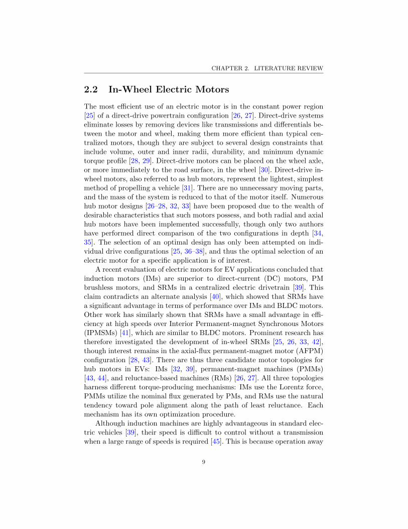
The most efficient use of an electric motor is in the constant power region[25] of a direct-drive powertrain configuration [26, 27]. Direct-drive systemseliminate losses by removing devices like transmissions and differentials be-tween the motor and wheel, making them more efficient than typical cen-tralized motors, though they are subject to several design constraints thatinclude volume, outer and inner radii, durability, and minimum dynamictorque profile [28, 29]. Direct-drive motors can be placed on the wheel axle,or more immediately to the road surface, in the wheel [30]. Direct-drive in-wheel motors, also referred to as hub motors, represent the lightest, simplestmethod of propelling a vehicle [31]. There are no unnecessary moving parts,and the mass of the system is reduced to that of the motor itself. Numeroushub motor designs [26–28, 32, 33] have been proposed due to the wealth ofdesirable characteristics that such motors possess, and both radial and axialhub motors have been implemented successfully, though only two authorshave performed direct comparison of the two configurations in depth [34,35]. The selection of an optimal design has only been attempted on indi-vidual drive configurations [25, 36–38], and thus the optimal selection of anelectric motor for a specific application is of interest.
A recent evaluation of electric motors for EV applications concluded thatinduction motors (IMs) are superior to direct-current (DC) motors, PMbrushless motors, and SRMs in a centralized electric drivetrain [39]. Thisclaim contradicts an alternate analysis [40], which showed that SRMs havea significant advantage in terms of performance over IMs and BLDC motors.Other work has similarly shown that SRMs have a small advantage in effi-ciency at high speeds over Interior Permanent-magnet Synchronous Motors(IPMSMs) [41], which are similar to BLDC motors. Prominent research hastherefore investigated the development of in-wheel SRMs [25, 26, 33, 42],though interest remains in the axial-flux permanent-magnet motor (AFPM)configuration [28, 43]. There are thus three candidate motor topologies forhub motors in EVs: IMs [32, 39], permanent-magnet machines (PMMs)[43, 44], and reluctance-based machines (RMs) [26, 27]. All three topologiesharness different torque-producing mechanisms: IMs use the Lorentz force,PMMs utilize the nominal flux generated by PMs, and RMs use the naturaltendency toward pole alignment along the path of least reluctance. Eachmechanism has its own optimization procedure.
Although induction machines are highly advantageous in standard elec-tric vehicles [39], their speed is difficult to control without a transmissionwhen a large range of speeds is required [45]. This is because operation away
9

CHAPTER 2. LITERATURE REVIEW
from the synchronous speed can decrease the efficiency of the machine [45].The synchronous speed is determined by the frequency of input three-phasepower. Thus, it is difficult to use a single power supply to drive an IMat both low (e.g. 5 [rpm]) and high (e.g. 5000 [rpm]) speeds due to themassive variation in supply frequency that would be necessary. Anotherdesign-related concern arises due to the fact that hub motors almost in-variably require an external-rotor configuration. External rotor IMs havean increased inertia, and are not as well investigated as the internal rotorconfiguration [46]. External-rotor IMs also face reduced airgap flux densitywhen compared to the identical configuration using an internal rotor, as insome other machines [47].
Permanent-magnet machines and RMs are both classified as flux-switching machines that share a common operating principle [37]. SwitchedReluctance Motors (SRMs) rely entirely on the variable reluctance of thealigned and unaligned positions of the rotor backiron [38], while BLDCs,Switched Permanent-magnet Motors (SPMs), IPMSMs, and AFPMs har-ness the nominal flux produced by embedded PMs to increase the active-pole flux density produced at each winding with minimal current [32, 37,41, 44]. Both types of flux-switching machine rely on the tangential compo-nent of pole flux density to generate torque, though they are separated by adistinct design choice between higher nominal pole flux and lower minimumpole flux. Torque is produced by the difference between the maximum andminimum flux levels, so both choices are valid, but have different results.PMMs tend to require lower driving currents, but they have to overcomethe negative torque produced by the PMs when the driving current is off.This is called cogging torque, and it arises between the PMs and the rotorteeth, reducing performance at low speed and generating unwanted noiseand vibration [48]. Cogging torque is difficult to mediate, but can be nearlyeliminated in PMMs through the use of anisotropic magnetized materials[49]. In contrast to PMMs, SRMs utilize cogging torque to generate rotation[50], eliminating it as a loss mechanism. Assuming that the motor’s con-troller successfully forces driving current to zero when demanded, there isno negative torque in an SRM.
The PM machine topology that is most commonly used by in-wheel mo-tors is the BLDC. Several BLDC motors have been designed for both hybrid-electric vehicles (HEVs) and EVs that meet or exceed minimum necessarytorque using 10− 15 [kW ] at 90-95% efficiency rated for 1000− 1200 [rpm][29, 51]. Commercial BLDC designs include safety considerations for mo-tor failure and vehicle handling due to increased unsprung mass [12, 28],while academic research has emphasized efficiency [52, 53] and thermal per-
10

CHAPTER 2. LITERATURE REVIEW
formance [54]. Few designers include mechanical durability analysis of anymotor topology [26], but several investigate control methodology, sizing, andperformance [26, 28, 32].
SRM hub motors are restricted to just five examples visible in the lit-erature [25, 26, 33, 42, 55], while there are over eight PM machines are tobe found [10, 27–29, 32, 51–53, 56]. Regardless, the SRM topology is moreuseful for volume production because of its inherent low cost, durability,ease of manufacture, and common material composition.
2.2.1 Materials for Electromechanical Devices
In-wheel motors utilize electrically-conductive, magnetically-permeable, andpolarized magnetic materials, each of which affect their efficiency and per-formance. Conductive materials represent the largest portion of the losses inmost motor topologies, and specifically in an SRM, since they make up thewindings on each pole of the motor. These windings may be composed ofcopper, or a superconductor. Copper is the most common winding material,and has a resistivity of 1.73 ·10−8 [Ω ·m]. In-wheel motors use winding opti-mization to maximize the density of copper windings, producing the highestpossible flux density with the least energy in the smallest volume.
Superconductors may be used as an alternative to copper, but theyhave an energy overhead due to their refrigeration requirement. Thereis not enough space in an in-wheel motor for a full refrigeration system.High-temperature superconductors can reduce the refrigeration requirement,but the 130K upper temperature limit of the most recent laboratory-gradeMercury-Barium-Calcium-Cuprate [57] is still in the range of liquid nitrogencooling. The highest-temperature commercial option is 344 YBCO, a three-ply Yttrium-Barium-Cuprate that can operate at 77K [58]. The cooling ofsuch a material, and the nitrogen supply problem, both represent significantissues that make superconductors for in-wheel motors unlikely.
Magnetically-permeable materials make up the motor backiron of anin-wheel motor, and determine hysteresis losses. Highly permeable mate-rials include grain-oriented silicon steel alloys, amorphous metal laminates,and sintered metallic powders. Silicon steel alloys are the original backironmaterial used in power transformers, and have since been replaced by amor-phous metal laminates in most high frequency applications. Silicon steelsare still used in some applications with low operating frequencies, but theynow have competition from sintered powder components, which are easier tomanufacture. Sintered metallic powders and composites have recently im-proved in performance [4], and now offer comparable performance to even
11

CHAPTER 2. LITERATURE REVIEW
the best laminates. Composites are cheaper than alloys, and can be used inthree-dimensional flux paths. The most common alloy materials used todayinclude iron-nickel and iron-cobalt metals, manufactured under the namesHiperco, Permendur, and Vacoflux.
Materials which retain a permanent magnetic polarization are called per-manent magnets. PMs include Ferrite, Samarium-Cobalt, Neodymium-Iron-Boron, and several other exotic materials. They can be used to reinforce thenominal flux or supply the reactive force in a motor and to suspend devicesand vehicles both actively and passively. Working with permanent magneticmaterials involves several challenges that range from cost and durability toperformance and mass. Aging, demagnetizing flux, vibration, and mount-ing difficulties can make working with PMs in industrial settings difficultwithout proper analysis. Permanent magnetic materials are most useful inisolated machines that operate at high frequencies, generate minimal de-magnetizing flux, and require high efficiency. A clever designer can use PMsto supply steady fields in situations where direct control is not necessary,reducing the electrical overhead of the device. Such applications includeelectrodynamic maglev and BLDC motors.
2.3 In-Wheel Automotive Suspensions
An in-wheel suspension system can be used to handle the unsprung massissue of in-wheel motors. Several novel systems have been suggested, includ-ing independent rotors and stators [10], additional motor bushings [14], andtraditional suspension tuning [59].
An independent rotor-stator machine is referred to as a split rotor-statormachine, given the division of the motor mass between the sprung and un-sprung segments of the vehicle. This approach to solving the hub motorhandling problem relies on sophisticated control of motor performance toensure safety and efficiency.
The addition of bushings to an in-wheel motor places the mass of themotor in parallel with that of the wheel. Bushings can be added between therotor and stator, or between the stator and outer casing. Bushings betweenthe rotor and stator will produce a variable airgap, reducing performanceand efficiency, while bushings between the stator and casing will increasethe fraction of the motor mass which is placed in parallel with the wheel.
Tuning of a traditional two degree-of-freedom (2DOF) suspension sys-tem to accommodate the increased unsprung mass of a hub motor suggests
12
CHAPTER 2. LITERATURE REVIEW
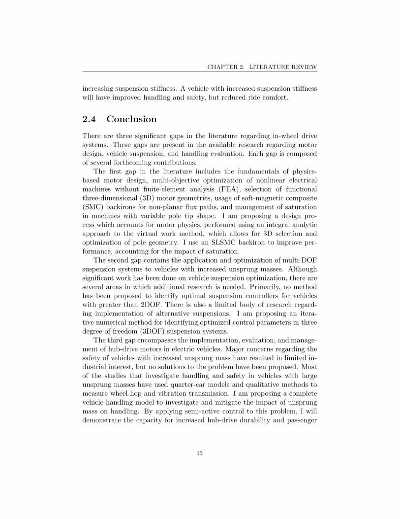
increasing suspension stiffness. A vehicle with increased suspension stiffnesswill have improved handling and safety, but reduced ride comfort.
2.4 Conclusion
There are three significant gaps in the literature regarding in-wheel drivesystems. These gaps are present in the available research regarding motordesign, vehicle suspension, and handling evaluation. Each gap is composedof several forthcoming contributions.
The first gap in the literature includes the fundamentals of physics-based motor design, multi-objective optimization of nonlinear electricalmachines without finite-element analysis (FEA), selection of functionalthree-dimensional (3D) motor geometries, usage of soft-magnetic composite(SMC) backirons for non-planar flux paths, and management of saturationin machines with variable pole tip shape. I am proposing a design pro-cess which accounts for motor physics, performed using an integral analyticapproach to the virtual work method, which allows for 3D selection andoptimization of pole geometry. I use an SLSMC backiron to improve per-formance, accounting for the impact of saturation.
The second gap contains the application and optimization of multi-DOFsuspension systems to vehicles with increased unsprung masses. Althoughsignificant work has been done on vehicle suspension optimization, there areseveral areas in which additional research is needed. Primarily, no methodhas been proposed to identify optimal suspension controllers for vehicleswith greater than 2DOF. There is also a limited body of research regard-ing implementation of alternative suspensions. I am proposing an itera-tive numerical method for identifying optimized control parameters in threedegree-of-freedom (3DOF) suspension systems.
The third gap encompasses the implementation, evaluation, and manage-ment of hub-drive motors in electric vehicles. Major concerns regarding thesafety of vehicles with increased unsprung mass have resulted in limited in-dustrial interest, but no solutions to the problem have been proposed. Mostof the studies that investigate handling and safety in vehicles with largeunsprung masses have used quarter-car models and qualitative methods tomeasure wheel-hop and vibration transmission. I am proposing a completevehicle handling model to investigate and mitigate the impact of unsprungmass on handling. By applying semi-active control to this problem, I willdemonstrate the capacity for increased hub-drive durability and passenger
13
CHAPTER 2. LITERATURE REVIEW
comfort. In summary, I am solving the problems presented by these gaps inresearch by providing the following:
• Evidence suggesting that a novel semi-anhysteretic in-wheel axial-fluxSRM with a split rotor-stator configuration using an SLSMC backironand a modified pole surface is the optimal electric propulsion systemfor passenger vehicles.
• A novel closed-form design approach based on a new integral induc-tance function, which can be mathematically optimized using themonotonicity principle.
• A 3DOF semi-active single-sensor suspension system which eliminatesthe yaw-type handling problem caused by increased unsprung mass.
14
Chapter 3
A Semi-AnhystereticAxial-Flux
Switched-Reluctance Motor
3.1 Introduction
This chapter presents a novel in-wheel SRM topology. The design is intendedto deliver high torque density and high efficiency to reduce the price of a widerange of electromechanical devices, including compressors, electric vehicles,turbines, and generators. We focus on the development of a motor whichwould improve the performance, range, and handling of electric vehicles.
3.1.1 Context of the Motor Design
Switched-reluctance motors are cheap, durable, and failsafe [60], but theydepend on high-accuracy sensors and controllers which have only recentlybeen developed [61]. Their simplicity, reliability, performance, and efficiencymake them highly competitive with other motor topologies for use in elec-tric vehicles [26, 27], while inviting creative design modifications to improveperformance further [15, 62–65].
The following sections will introduce the design, modelling, control, andperformance of the in-wheel SRM. The topology of the motor is first identi-fied using qualitative geometric and physical motivations, which also permitthe selection of motor materials. The nature and behaviour of the energyconversion process is then described by a set of models, which are used toprovide quantitative boundaries for the design process. A range of designtools and modelling techniques are compared, and the optimal technique isselected. Energy conversion models are then applied using the chosen tech-nique, and a quantitative set of design equations is produced. An iterativeprocess based on the same set of equations is used to optimize the design.Finally, a control strategy is developed, and the performance of the motoris evaluated using several static and dynamic criteria.
15

CHAPTER 3. A SEMI-ANH. AXIAL-FLUX SRM
3.2 Selection of the Motor Topology
This section describes the purpose and methodology of the qualitative motordesign process in the context of topology and material selection. Whilequantitative design considerations can be described by performance indices,qualitative design considerations do not have precise numerical equivalents.Qualitative design, performed prior to quantitative design, will identify thedesign parameters to be used in the quantitative design process.
The optimal SRM geometry can be identified using a qualitative ap-proach [66] to Maxwell’s Stress Tensor [67], or by examining the reluctance[68] and total flux linkage [69] of a MEC model. Airgap geometry determinesthe shape of the torque and radial force curves [62], as in permanent-magnetmachines [70]. Numerous airgap modifications including tooth-notching,tooth chamfering, teeth-pairing, and rotor skewing have been attempted[71], but most modifications lead to decreased average torque [62], thoughsome reduce torque ripple as well [36]. Teeth-pairing is the only torque pro-file shaping mechanism which has been shown to increase average torque influx-switching machines [71]. Other design techniques improve the availabletorque by reducing the size of the airgap [15] or by altering the stack length[72]. Rotor skewing is the simplest mechanism to cancel ripple harmonicswhile maintaining peak torque, but back-EMF-guided current shaping mustbe implemented to avoid creating more torque ripple due to the mutualinductance profile [73]. Static torque ripple can be reduced by up to 25%with optimal pole tip shaping [36, 62] or variation of the number of phases[42]. Motor harmonics can also be produced by unbalanced radial forces [65],which can be balanced by doubling the number of poles, forcing flux reversalin the stator [65], or by dual-stator pairing [15].
The variability of SRM geometry has resulted in a range of novel designs[15, 62–65] that include motors with segmental rotors [74], higher numbersof rotor poles [72, 75], shaped pole tips [36, 62, 76], rotor skew [73], multi-phase excitation [77], and 3D flux paths [78]. The difficulty in evaluating therelative performance of these designs, and in conceiving better ones, stemsfrom a lack of understanding of the energy conversion mechanisms in anSRM [75]. Some confusion is caused by claims that saturation will increaseperformance [79], without clarification that saturation requires more energy.Complete description of the effect of saturation on reluctance torque in MECmodels [80] is often necessary, but can be avoided in machines with lowerflux [77]. Saturation reduces the maximum inductance near the aligned posi-tion, decreasing the peak torque, and is usually avoided if possible [77]. Thequalitative design process is intended to clarify any confusion by providing
16

CHAPTER 3. A SEMI-ANH. AXIAL-FLUX SRM
a fundamental theory of SRM geometry that can be used to compare thefull range of novel motor configurations, and design parameter variations,without the need for a precise model.
The set of motor design parameters includes pole size, pole tip shape,pole configuration, phase length, phase alignment, phase voltage, stacklength, outer radius, winding thickness, and wire diameter. Qualitativemethods may be used to establish the range and boundaries of each pa-rameter using the saturation point, frequency dependence of eddy-current,rise-time of the winding current, material cost, winding-current heat produc-tion, and maximum machine size. The quantitative design process can thenidentify the optimal value of each parameter by evaluating the performanceof each design variation. The effect of each design parameter on the designcan be calculated using the performance index. The effect of each parameterwill be based on the model, which can be either linear or nonlinear. A linearmodel can be shown to produce a monotonic change in the performance in-dex for all design variations, while a nonlinear model may produce a changein any direction. If a nonlinear model produces a monotonic change, thena linear model will produce the same result. The qualitative design processcan therefore be used to speed up the optimization process if it determinesthat a set of design parameters is monotonic.
The qualitative design process may be approached using linear circuitanalysis and an energy functional, but this procedure is generally one-dimensional. Maxwell’s stress tensor, as derived in Appendix A, is moreaccurate, and inherently calculates forces in three-dimensions. The tensoris given by
←→T = ~E ~Em + ~Bm ~B −
1
2
←→I ( ~E · ~Em + ~Bm · ~B) (3.1)
where B is the magnetic field, E is the electric field,←→I is the identity tensor,
and the subscript m refers to the backiron. The stress tensor in a purelymagnetic system is equivalent to
←→T =
1
µ0
B2x −B2/2 BxBy BxBzByBx B2
y −B2/2 ByBzBzBx BzBy B2
z −B2/2
(3.2)
where x, y, and z refer to the coordinate axes, and B2 = B2x + B2
y + B2z .
The components of the normal force, as shown on the diagonal of (3.2),depend on the component of the magnetic field that is perpendicular to thesurface, while the components of the tangential force depend on at leastone factor of the field that is parallel to the surface. Since the backiron
17
CHAPTER 3. A SEMI-ANH. AXIAL-FLUX SRM
does not carry a significant surface current, the continuity relation requiresthat the tangential field is continuous across the backiron interface, butit also requires that the parallel field is discontinuous due to the higherrelative permeability of the backiron, µr . The condition on the parallel-field components occurs due to the continuity of the applied field, or fieldintensity, H :
H||,air =1
µ0B||,air = H||,backiron =
1
µ0µrB||,backiron (3.3)
B||,air =1
µrB||,backiron (3.4)
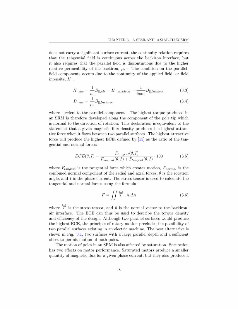
where || refers to the parallel component . The highest torque produced inan SRM is therefore developed along the component of the pole tip whichis normal to the direction of rotation. This declaration is equivalent to thestatement that a given magnetic flux density produces the highest attrac-tive force when it flows between two parallel surfaces. The highest attractiveforce will produce the highest ECE, defined by [15] as the ratio of the tan-gential and normal forces:
ECE(θ, I) =Ftangent(θ, I)
Fnormal(θ, I) + Ftangent(θ, I)· 100 (3.5)
where Ftangent is the tangential force which creates motion, Fnormal is thecombined normal component of the radial and axial forces, θ is the rotationangle, and I is the phase current. The stress tensor is used to calculate thetangential and normal forces using the formula
F =
∫∫ ←→T · n dA (3.6)
where←→T is the stress tensor, and n is the normal vector to the backiron-
air interface. The ECE can thus be used to describe the torque densityand efficiency of the design. Although two parallel surfaces would producethe highest ECE, the principle of rotary motion precludes the possibility oftwo parallel surfaces existing in an electric machine. The best alternative isshown in Fig. 3.1, two surfaces with a large parallel depth and a sufficientoffset to permit motion of both poles.
The motion of poles in an SRM is also affected by saturation. Saturationhas two effects on motor performance. Saturated motors produce a smallerquantity of magnetic flux for a given phase current, but they also produce a
18

CHAPTER 3. A SEMI-ANH. AXIAL-FLUX SRM
Figure 3.1: Best physical alternative pole configuration.
larger quantity of torque because saturation increases the fringing flux, as inFig. 3.2. There is a specific winding current which will produce the highestECE at each rotation angle for a given nonlinear backiron material, but thiscurrent can only be calculated during the quantitative design process. Insummary, the qualitative design process harnesses physical motivations tomake important design decisions, but cannot be used to define the values ofdesign parameters without the quantitative design process.
Figure 3.2: Effect of saturation on flux density.
19

CHAPTER 3. A SEMI-ANH. AXIAL-FLUX SRM
3.2.1 Selection of Design Geometry using Qualitative Phys-ical Motivations
Geometric design parameters can be described qualitatively using eitherempirical or physical equations. Empirical design equations are availablefor several standardized motors, but they are not sensitive to small designmodifications, though they may include the stack length, number of poles,outer radius, and backiron saturation point. The physical approach to motordesign responds to all design modifications, including pole shape, gap shape,winding geometry, driving current, and phase activation strategy, and canbe used to select the design itself. We design a novel split rotor-stator in-wheel motor using the physical approach for this reason. The considerationsinvolved in a qualitative physical design process for such a motor are asfollows:
1. Maximum Torque: torque is produced by the gradient of the effectiveinductance1 from unaligned to aligned positions. The unaligned po-sition must therefore have a minimum inductance, while the alignedposition must have a maximum inductance. The unaligned positionshould therefore have no overlap between rotor and stator poles, whilethe aligned position should correspond to complete overlap.
2. Torque Shape: average torque is a function of the aligned and un-aligned inductances. The total quantity of torque produced per phaseis therefore not a function of the pole shape, subject to the consider-ations of maximum torque and saturation. The shape of the torquecurve can be altered by changing the pole tip shape, without affectingthe torque density of the motor.
3. Backiron Material: saturation may improve performance in machineswith low ECE, but represents a limit on the inductance of the alignedposition. The backiron should be able to carry the total flux withoutreaching saturation, but should saturate near the pole tip to so as toincrease the fringing flux. A higher saturation point will improve per-formance if the permeability of the backiron is the limiting factor, butif the machine no longer reaches the saturation point it will experiencereduced ECE and lower torque density.
1Nonlinearity due to saturation obscures the precise definition of the inductance, butthe concept is useful during the design process.
20

CHAPTER 3. A SEMI-ANH. AXIAL-FLUX SRM
4. Pole Size: any motor with aligned and unaligned positions2 will pro-duce more torque given a larger pole size, assuming that the unalignedrotor position has no overlap with an active stator pole. The maxi-mum pole size possible in a specific motor volume is therefore optimal.This consideration is reinforced by a simple calculation of copper loss.The resistance of a winding is given by
R = ρclwindawind
= ρ2√πApole
awind(3.7)
where ρc is the resistivity of copper, lwind is the length of the winding,awind is the cross-section of the winding, and Apole is the cross-sectionalarea of the pole face. The average torque for two motors with identi-cal unaligned inductances will be a function of the magnitude of thealigned inductance. It will also be a function of the aligned field-energy 1
2φ2<, where φ is flux and < is reluctance. Given pole areas
A2 = 2A1, with A2 as the area of pole 2 and A1 as the area of pole1, equal aligned field-energies suggest that φ2 =
√2φ1. The magneto-
motive force (MMF) is given as F = ΦR = NI, where N is the numberof turns in a coil and I is the current in that coil. Solving for currentresults in
NI1 = Φ1<1 = Φ1lfluxµA1
(3.8)
NI2 = Φ2<2 = Φ2lfluxµA2
=√
2Φ1lfluxµ(2A1)
(3.9)
where lflux is the path length and µ is the permeability of the material.We see that I1 =
√2I2. The resulting power requirement is
P1 = I21ρ
2√π
a
√A1 (3.10)
P2 = I22ρ
2√π
a
√A2 =
1
2I2
1ρ2√π
a
√2A1. (3.11)
Therefore P2/P1 = 1/√
2 = 0.7071. As the area increases, power lossesdecrease.
5. Pole Tip Shape: pole tip shaping along the tangential direction typ-ically reduces the average torque produced by a motor, suggesting
2Induction motors and solenoids are therefore not affected by this design consideration.
21

CHAPTER 3. A SEMI-ANH. AXIAL-FLUX SRM
that shaping should only occur if motivated by a design requirement.Shaping along the radial and axial directions has not been investi-gated thoroughly to the best of our knowledge, yet it is important toconsider.
6. Pole Configuration: the motion of an activated pole produces the back-EMF, shapes the backiron’s magnetic hysteresis cycle, and prescribesthe optimal shape of the phase current. Back-EMF is produced by thechange in flux through a winding, and is therefore unavoidable. Theback-EMF does not guide the design process. The hysteresis cycle andassociated phase current will, however, have a direct affect on motorlosses. Reducing the frequency and magnitude of hysteresis will thusincrease the efficiency of the motor.
7. Phase Length: a longer backiron segment per phase will both reducethe inductance of the aligned position and increase hysteresis losses.The minimum backiron length is therefore desired.
8. Phase Number: a larger number of poles and phases will result in alarger average torque if the controller can achieve single-pulse control:
τavg =NsNr∆W
4π, (3.12)
where τavg is the average torque, Ns and Nr are the number of poleson the stator and rotor, and ∆W = Waligned−Wunaligned . The energydifferential ∆W is directly dependent on the number of windings oneach pole and on the reluctance of the motor as it moves from theunaligned to aligned position. The ECE for the energy contained inthe magnetic field is higher near the unaligned position, when thereis only a small overlap between the rotor and stator poles. The sizeof the overlap can be reduced by increasing the number of poles. Alarger number of poles will thus increase the amount of time that theactive phase spends near the overlap point, producing more torque.
9. Phase Alignment: a rotating machine can be either radial or axial.Machines can also be designed in the inner- and outer-rotor configura-tions. Displacement of the rotor and stator beyond the length of theairgap is only possible in an axial configuration, and an outer-rotorarrangement will maximize the available winding space3.
3The radial direction is more constrained than the axial direction in a hub motor, whichlimits the length of axial inner-rotor windings. A motor with a shorter stack length could
22

CHAPTER 3. A SEMI-ANH. AXIAL-FLUX SRM
Further evidence in support of the axial-flux configuration can befound in the motor geometry. For a constant motor volume, the ge-ometry of radial and axial flux machines can be described by
rradial =raxial
2=rvolume
2(3.13)
lradial = 3laxial = lvolume (3.14)
where r is the radius, l is the stack length, radial refers to the ra-dial motor configuration, axial to the axial motor configuration, andvolume to the outer boundary to both radial and axial configurations.The rotor-stator interface surface in a radial machine can be definedby
Aradial = 2πrradiallradial
= 2πrvolume
2lvolume. (3.15)
The rotor-stator interface surface in an axial machine can be definedby
Aradial = 2πr2axial = 2πr2
volume. (3.16)
Thus the axial configuration contains a larger interface surface forrvolume > 0.5lvolume, assuming a radial rotor-stator interface radius of0.5rvolume.
The design considerations that we have developed can be reduced to aset of conclusions:
1. Performance is proportional to the size of the rotor-stator interfacesurface. The interface surface is proportional to the motor volume fora given design.
2. The number of phases is chosen by optimizing the performance underthe Pole Size and Phase Number design considerations. A dynamicoptimization procedure is necessary to identify the optimal number ofphases that will produce the highest torque and efficiency.
3. Radial and axial pole tip shaping along the direction perpendicular tothe motion of the rotor may improve performance.
be designed using the inner rotor arrangement if the axial direction was more constrained,but it would still make poor use of the rotor-stator interface surface.
23

CHAPTER 3. A SEMI-ANH. AXIAL-FLUX SRM
We have used these conclusions to develop a qualitative design whichincludes:
1. A short flux path
2. An axial-flux motor configuration
3. An outer-rotor topology
4. No flux reversal
An example of a motor design which incorporates these characteristicsis shown in Fig. 3.3. Such a motor is referred to as an axial-flux switched-reluctance motor (AFSRM). Reversal occurs when current changes directionin a winding, or when windings from the same phase interact sequentiallyand in opposing directions on a single segment of backiron. This conditioncan be avoided by careful control with a large number of electrical cyclesper mechanical cycle.
Figure 3.3: Qualitative Motor Design Schematic.
24

CHAPTER 3. A SEMI-ANH. AXIAL-FLUX SRM
3.2.2 Material Selection
The materials chosen during the qualitative motor design process should notaffect the topology of the motor, and should be selected based on the Back-iron Material design consideration. A material’s performance is secondaryto its applicability to a given motor design. The optimal material choicewill therefore depend on the specific motor application.
Background
Electric motors use engineered materials to optimize the efficiency of fieldwindings. Several different options are available to designers that providecharacteristics for different applications. Typical motor topologies use fer-rous laminates that have low core losses, but alternative materials are avail-able that also maximize the saturation flux density.
Standard motor laminates are stacked with thin insulating layers thatmake up as much as 5% of the total mass of the back-iron. Thinner layersreduce eddy currents, but manufacturing limits make the current laminationdimensions difficult to improve. The adhesion of each layer is also depen-dent on the sintering technique used, which can affect the resistance of thecomposite device. Sintered edges can link two layers and make the effectivethickness double.
Steels used in each layer are designed to have minimum electrical con-ductivity, maximum magnetic permeability, and the highest saturation fluxdensity. Carbon steel is often augmented with 0.5-3.5% silicon content toreduce electrical conductivity. Anisotropic silicon steel is also annealed toensure quality. Several grades are available, typically described by the Amer-ican Iron and Steel Institute (AISI) system. Low grades like M45 and highgrades like M15 are all named using the losses caused by 1.5 T fields at 60Hz. M15 steel will thus have a loss of 1.5 W/lb. Commercially availableimprovements on traditional silicon steel include Arnon 5 and 7, which canhave less than half of the losses seen otherwise.
Components that require higher saturation flux densities use iron-cobaltalloys. These materials are more expensive due to the large amount of cobaltrequired to produce them. Standard alloys like Hiperco-50, as manufacturedby Carpenter, have a component breakdown of 49% Fe, 48.75% Co, 1.9%V, 0.05% Mn, 0.05% Nb, and 0.05% Si. Permendur, Permendur V, andVacoflux 50 are similar.
Soft magnetic composites can be used when the high two-dimensionsal(2D) performance of laminates is not required. SMCs are constructed using
25
CHAPTER 3. A SEMI-ANH. AXIAL-FLUX SRM
Fe powder that is mixed with epoxy resin, compacted, and then sintered.Core losses in SMCs are higher than in laminates, but they are cheaper,easier to work with, and may even be competitive when a 3D motor topologyis used. Magnetic flux can pass in any direction through an SMC core,expanding the range of optimizable geometric parameters. SLSMCs areparticularly close to reaching the effective permeability provided by highquality laminations. Accucore is the best commercially available SMC, andhas losses of 9 W/kg at 1 T and 100 Hz.
Amorphous ferromagnetic alloys, superconductors, and nanostructuredmaterials are the most advanced materials available. Amorphous alloys canbe produced that have losses between 0.125 and 0.28 W/kg at 1 T and 50 Hz.This is achieved by flash-freezing molten metals into nanocrystalline frozenliquid. Superconductors can be used to remove resistive losses from powertransmission components, but require extensive cooling measures. Nanos-tructured materials attempt to avoid the cooling requirement of supercon-ductors by utilizing the odd properties of graphene. Graphene nanotubeswith a thickness of 1-100 nm can be grown that conduct massive currents,but lengths of only a few millimeters are currently possible.
Materials for the In-Wheel AFSRM
The cost, availability, strength, and performance of materials are used toevaluate their applicability to a given design. Exotic materials are generallytoo costly to incorporate in machines that are intended for high productionvolumes, but the characteristics of laminates, SMCs, and amorphous metalsare an important part of the motor design process. Material selection shouldbe carried out in parallel with the choice of the motor topology, guideddirectly by the design methodology.
The methodology of the in-wheel AFSRM design process suggests thata 3D flux path is optimal. A 3D flux path is difficult to achieve with tradi-tional laminates, which become expensive in complicated geometries due tomanufacturing limitations. Materials without similar limits should be usedto reduce cost. Amorphous metals are expensive and difficult to produce,so SMCs will be considered.
Although SMCs are known to have higher core losses than other backironmaterials, they are low cost and can be manufactured easily for a variety ofgeometries. Given the geometric flexibility of SMCs, the important param-eter to consider for SMC selection is performance.
Backiron material performance can be summarized by the remanence,coercivity, and saturation point. The remanence represents the strength of
26

CHAPTER 3. A SEMI-ANH. AXIAL-FLUX SRM
the magnetic field which persists after the applied field has been removed.The coercivity represents the strength of the opposing applied field that isnecessary to remove the remanent magnetization. High performance mate-rials for motor backiron applications will have low remanence and coercivityto reduce the energy absorbed by the magnetic hysteresis cycle. The shapeof the hysteresis cycle is given by the saturation point. A material with ahigh saturation point is desired to produce a high-performance motor.
The SMC with the best performance, highest saturation point, and low-est core loss is found to be an SLSMC [4]. An SLSMC is developed usingsquare segments of thin, high performance magnetic steel, sintered togetherwith an electrically-insulating bonding agent. SLSMCs have similar per-formance to M19 electrical steel, but retain the low cost and geometricflexibility of other SMCs.
A modular, low cost motor design has thus been identified for the in-wheel AFSRM application using a set of qualitative design considerationsand material choices. The optimal AFSRM design can now be determined bydeveloping a detailed model of the motor’s electromagnetic characteristics.
3.3 Modelling of the AFSRM
3.3.1 Modelling for Optimal Design
This section presents a model that accurately describes the geometric, elec-tromagnetic, and thermal characteristics of the AFSRM topology, highlight-ing the effect of motor geometry on the energy conversion process. ModernSRM models are composed of a wide array of static, dynamic, and controlequations [69, 79] that have been unified for the purpose of optimal ma-chine design [38]. Modern models account for saturation [77], power factorand back-EMF [79], and may be developed using linear magnetic circuits[81], FEA [67], or permeance functions [5]. One highly useful modern ap-proach takes the form of an analytic set of equations based on an integralpermeance function [5]. The permeance function provides a higher degreeof accuracy compared to more traditional linear magnetic equivalent circuit(MEC) models [81, 82] and has similar geometric accuracy to the MaxwellStress Tensor [67]. Accuracy is also dependent on the model’s agreementwith the geometry of the machine [67], its torque-producing fringing flux[15], and the effect of magnetic saturation [82]. Verification of model accu-racy is commonly achieved using FEA [6, 62, 76], though a full electricalmodel and control system is needed to evaluate dynamic behaviour [31, 32,67].
27

CHAPTER 3. A SEMI-ANH. AXIAL-FLUX SRM
A performance index is used to measure the effect of each design parame-ter on the AFSRM model, and the full range of electrical, magnetic, thermal,and mechanical losses is considered. A comparison of linear magnetic equiva-lent circuits, permeance functions, FEA, and vector-fields is performed. Thecomparison is then used to select the tool which can best describe the effectof each loss on the energy conversion process in the AFSRM. The completemodel is finally adapted to produce both static and dynamic descriptions ofthe reluctance, inductance, torque, and heat generated by the motor.
3.3.2 Modelling of Losses in Electric Motors
The losses in an electric motor may originate from electrical, magnetic, ther-mal or mechanical sources. Electrical losses in hub motors can be brokeninto alternating current (AC) and DC components, caused by eddy-currents,resistivity, the skin effect, and the proximity effect. The primary loss isdue to the resistivity of stator windings, but secondary losses are also pro-duced by the proximity effect, which can have a significant impact on motorperformance. Thermal losses may occur due to increased resistivity as acomponent of the primary loss. Unexplained behaviours caused by externalmagnetic fields and material irregularities make up for the final fraction ofthe electrical losses.
Magnetic losses are broken into static and dynamic components, whichare caused by magnetization, hysteresis, saturation, and material irregular-ities. The primary magnetic loss is due to hysteresis, which is a dynamicform of magnetization seen in motors which change the polarity of theirfield windings. Saturation may be considered a secondary loss, but it canbe beneficial in specific cases.
Mechanical losses include windage and rolling friction. Windage lossesare produced by viscous friction and turbulence in the air surrounding therotor, while rolling friction losses are produced by lubricant and deformationat the contact points of each bearing. Both of these losses are typicallyminimal compared to the electrical and magnetic losses. A performanceindex can be used to calculate the precise impact of each loss on the motor.
Efficiency is selected as the main performance index because it is di-rectly influenced by the geometry, circuitry, and materials in the motor.Several other metrics can be included in multi-objective optimizations, butthis design will focus on efficiency, with weight and cost as secondary con-
28

CHAPTER 3. A SEMI-ANH. AXIAL-FLUX SRM
siderations. Efficiency is typically formulated as:
η =PoutPin
=Pout
Pout + Pohm + Physt + Peddy + Pfriction + Pwindage(3.17)
where Pout is the mechanical output power of the motor, Pin is the powerthat is delivered to the motor, Pohm is the power lost to linear resistivity,Physt is the power lost to magnetic hysteresis, Peddy is the power lost to eddycurrents, and Pfriction and Pwindage are the power lost due to dissipativemechanical forces . Power is defined by:
Pout = τω (3.18)
where τ is the torque, and ω is the angular speed of the motor. Efficiency istherefore a function of rotor velocity, which indicates that motor losses willbe as well. Identifying the dynamic behaviour of each loss will improve themodel.
3.3.3 Electrical Losses
Electrical losses can be broken into AC and DC components. The AC com-ponent is a function of winding size, wire diameter, and rotational frequency.The DC component is a function of wire length, wire cross-section, and re-sistivity. Additional losses can be produced by variations in the externalmagnetic field, or by imperfections in the motor components, and are re-ferred to as stray losses. The AC and stray losses are commonly referred totogether as eddy currents.
The modern use of the term ‘eddy currents’ refers to the sum of the skinand proximity effects, but it is not limited to those effects alone. Circulatingcurrents produced as part of the stray losses also contribute to the fraction ofthe winding losses known as ‘eddy currents’. For this reason, the sum totalof the AC losses calculated hereafter omits the term ‘eddy currents’, and isinstead made up of the DC resistance, skin effect, proximity effect, and straylosses. A fortunate orthogonality [83] allows the independent calculation ofthe contribution to the AC resistance by the skin and proximity effects.The electrical losses can therefore be determined using a known excitationfrequency, motor geometry, and material composition.
29

CHAPTER 3. A SEMI-ANH. AXIAL-FLUX SRM
3.3.3.1 DC Losses
DC losses are a function of the winding resistance:
R =ρlwindAwire
(3.19)
where ρ is the resistivity, lwind is the length of the wire, and Awire is thecross-sectional area of the wire . Resistivity is temperature dependent, andof the form
ρ(T ) = ρref (1 + γ(T − Tref )) (3.20)
where ρref is the reference resistivity at 20 [C], T is the temperature , Trefis the reference temperature at which the resistivity is known, and γ is thetemperature coefficient of the wire. The temperature coefficient of copperis approximately 0.004.
3.3.3.2 Skin Effect
The first component of the AC losses is the skin effect. Alternating currentresponds to the uneven magnetic field inside a wire, and is pressed toward theouter edges where the opposing field is weakest. The higher the frequencyof current reversal, the farther the current is pushed toward the edge of thewire. The skin effect can be derived from the complex plane-wave equationfor the electric and magnetic fields in matter, shown in Appendix B. Theskin depth of a conductor is found by inverting the complex component ofthe wave number, giving the depth to which the field amplitude reduces bya factor of 1/e:
δ =1
ω√
εµ2
√√1 + ( σεω )2 − 1
(3.21)
where µ is the permeability, ε is the permittivity, σ is the conductivity, andω is the angular frequency. Assuming a good conductor where σ εω,
δ =1
ω√
εµ2
√σεω
=1√
µ2
√ωσ
=1√
µ2
√2πfσ
=1√µσπf
(3.22)
where f is the frequency of rotation.
30

CHAPTER 3. A SEMI-ANH. AXIAL-FLUX SRM
3.3.3.3 Proximity Effect
The second component of the AC losses is the proximity effect, which hasbeen calculated using both precise and approximate methods for round andsquare conductors. A review of the proximity effect is performed by [84],but the most modern analytical approach is presented by Nan and Sullivan[85]. Nan summarizes the approaches used by Dowell [86], Stoll [87], andFerreira [83] but concludes that a slightly modified Dowell approach is boththe easiest and most accurate to apply. The combined result of the work byDowell and Ferreira is then presented as:
RACRDC
= ξ′[
sinh 2ξ′ + sin 2ξ′
cosh 2ξ′ − cos 2ξ′+ η2 2
3(m2 − 1)
sinh 2ξ′ − sin 2ξ′
cosh 2ξ′ + cos 2ξ′
](3.23)
where ξ′ = ξ√η, ξ =
√πd
2δ , η = Nlab , Nl is the number of conductors per layer,
a is the width of each conductor, b is the window width, and m is the numberof layers. The driving current is required to be sinusoidal for this method tobe valid [85]. Non-sinusoidal currents can be analyzed using Fourier seriesdecomposition, but the signal must be AC in order to produce a proximityeffect. The novel motor topology developed in this chapter does not usean AC current, though it does use a DC current with variable amplitude.The DC current is therefore broken into AC and DC components, which aretreated separately. The energy losses in a winding can be seen in Fig. 3.4for different treatments of the current and resistance.
3.3.4 Magnetic Losses
Magnetic losses in the backiron have static and dynamic terms similar tothe AC and DC components of electrical losses. Static backiron losses area function of the magnetization and saturation effects, while dynamic lossesare also functions of time. A dynamic loss calculation includes the loss thatwould be seen in a static calculation, but also considers transient physicalphenomena. Backiron losses are therefore dependent on material propertiesand excitation frequency, and are a direct function of the nonlinear magne-tization curve.
Nonlinear magnetic saturation has a strong effect on the performance ofelectrical machines. The effect can be described by a permeability function,and creates an upper limit on the magnetic flux density (B) in a nonlinearmaterial. The permeability can be derived from the flux density as a func-tion of the field intensity (H), creating a BH curve. BH curves contain thequasi-static magnetization behaviour of materials, but do not account for the
31

CHAPTER 3. A SEMI-ANH. AXIAL-FLUX SRM
Figure 3.4: Losses due to AC and DC resistance in an accelerating motor.
32

CHAPTER 3. A SEMI-ANH. AXIAL-FLUX SRM
dynamics involved in a magnetization cycle, also known as magnetic hystere-sis. Dynamic BH curves can be developed using semi-empirical models, astrue physical models are not yet available. The essential concept involved ina semi-empirical model is that it relies on numerical simulation. Such simu-lations can be implemented directly using FEA, or developed independentlyusing prescribed inputs.
The choice between direct and independent models is influenced by theshape of the dynamic BH curve. Curves with low remanence and coercivityare candidates for independent analysis because their dynamic magnetiza-tion behaviour is similar a static BH curve. Curves with high coercivityor remanence are poor candidates for independent analysis because theirdynamic permeability is strongly dependent on magnetization history. In-dependent models can be used to calculate transient losses quickly, but havelow accuracy. Direct FEA models have high accuracy, but also have a highcomputational overhead which can be prohibitive in transient simulations.Time-harmonic FEA can be used to reduce this overhead in specific situa-tions.
The empirical Stienmetz function is a popular alternative to dynamicmagnetization calculations, but it requires experimental data to be imple-mented. It is a non-physical model with two fit parameters
Physt = kBxf (3.24)
where k is the first fit parameter, x is the second fit parameter, B is thepeak magnetic flux density, and f is the frequency of the hysteresis cy-cle. The Stienmetz model requires a sinusoidal input frequency, thoughnon-sinusoidal inputs can be handled using Fourier decomposition. No con-sideration of minor or partial hysteresis loops is included. The Stienmetzapproach is therefore only useful for empirical modelling, and can be highlyinaccurate in specific situations. True dynamic models are preferred becausethey are more accurate, can be developed without experimental data, andhave some physical relevance.
The two most popular dynamic treatments of hysteresis are the Preisachand Jiles-Atherton (JA) models. The Preisach model is an entirely phe-nomenological approach, with no innate physical meaning, while the JAmodel is based on electrodynamic behaviours and the Langevin function.We adopt the JA model due to its more direct treatment of physical per-formance, and its efficient parameter selection process. A new algorithmfor the JA model is implemented using the combined work of Leite [88],Izydorczyk [89], Sadowski [90], and Zirka [91]:
33

CHAPTER 3. A SEMI-ANH. AXIAL-FLUX SRM
1. Global Parameters:
Magnetic permeability in vacuum: µ0
Magnetic permeability at B = 0: µZ
Resistivity: ρC
Coercivity: Hc
Remanent Magnetization: Mr
Backiron Density: ρSLSMC
Lamination Thickness: dlam
2. Model Parameters:
c = µZ−1Mr/Hc−µZ
k = Hc
Shape (fitting parameter): a
α = c(1+c)·(µZ−1)·(3a−1)
3. Model Inputs:
Flux Density: B
Flux Density Rate: dBdt
Initial Field Intensity: H0
Previous Field Intensity: H ′
Field Intensity: H = H0 on first iteration, H = H ′
afterward.
4. Model Expressions:
Excess Loss Parameter: kexc = k1(1 + k2B2)
Loop Direction Parameter: δ = 1 if dBdt ≥ 0, δ = −1 otherwise.
5. Magnetization Process:
Dynamic Field Intensity: Hdyn =d2lam12ρC
dBdt + kexcδ
dBdt
2
34
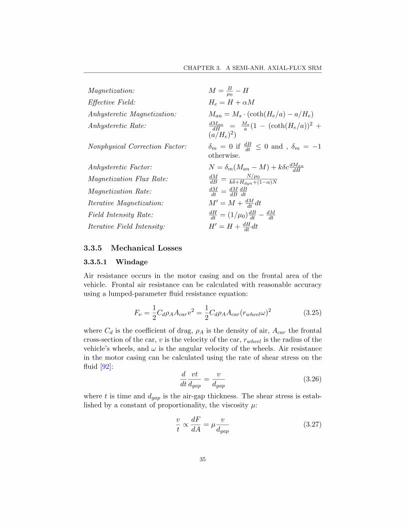
CHAPTER 3. A SEMI-ANH. AXIAL-FLUX SRM
Magnetization: M = Bµ0−H
Effective Field: He = H + αM
Anhysteretic Magnetization: Man = Ms · (coth(He/a)− a/He)
Anhysteretic Rate: dMandH = Ms
a (1 − (coth(He/a))2 +(a/He)
2)
Nonphysical Correction Factor: δm = 0 if dBdt ≤ 0 and , δm = −1
otherwise.
Anhysteretic Factor: N = δm(Man −M) + kδcdMandH
Magnetization Flux Rate: dMdB = N/µ0
kδ+Hdyn+(1−α)N
Magnetization Rate: dMdt = dM
dBdBdt
Iterative Magnetization: M ′ = M + dMdt dt
Field Intensity Rate: dHdt = (1/µ0)dBdt −
dMdt
Iterative Field Intensity: H ′ = H + dHdt dt
3.3.5 Mechanical Losses
3.3.5.1 Windage
Air resistance occurs in the motor casing and on the frontal area of thevehicle. Frontal air resistance can be calculated with reasonable accuracyusing a lumped-parameter fluid resistance equation:
Fν =1
2CdρAAcarv
2 =1
2CdρAAcar(rwheelω)2 (3.25)
where Cd is the coefficient of drag, ρA is the density of air, Acar the frontalcross-section of the car, v is the velocity of the car, rwheel is the radius of thevehicle’s wheels, and ω is the angular velocity of the wheels. Air resistancein the motor casing can be calculated using the rate of shear stress on thefluid [92]:
d
dt
vt
dgap=
v
dgap(3.26)
where t is time and dgap is the air-gap thickness. The shear stress is estab-lished by a constant of proportionality, the viscosity µ:
v
t∝ dF
dA= µ
v
dgap(3.27)
35

CHAPTER 3. A SEMI-ANH. AXIAL-FLUX SRM
where F is the shear force. If the area of the rotating surface is defined asA = 2πrsurf laxial and v = rsurfω, the above equation can be integrated toresult in
F =2πµr2
surfωlaxial
dgap(3.28)
where laxial is the axial length, and rsurf is the radius of the rotor. Definingthe power absorbed by rotating air to be Pair = Frsurfω, the expressionbecomes
Pair =2πµr3
surfω2laxial
dgap. (3.29)
This equation can be expressed using a Reynolds number, but the currentformat is more accessible. This equation ignores turbulence and does notaccount for surface irregularity. The equation should also be modified toaccount for the axial configuration of the motor. A second term is addedthat represents the shear resistance due to the sides of the rotor, wherethe previous expression only gave a value for the circumference. The finalexpression is therefore composed of two forces:
τ = τcirc + 2τside =2πµr3
surfωlaxial
dcirc+ 2
2πµr4surfω
4dside(3.30)
where τcirc is the torque produced by windage on the circumference of therotor, τside is the torque produced by windage one the top and bottom ofthe rotor, dcirc is the radial clearance of the rotor, and dside is the axialclearance of the rotor.
3.3.5.2 Bearing Losses
There are three primary bearing support mechanisms:
• Mechanical rolling elements
• Elastohydrodynamic fluid compression
• Electromagnetic suspension
The mechanical rolling-element bearing (REB) is the most common supportmechanism for both vehicle axles and motors. REB losses are primarilylinear as a function of load. The behaviour of a REB is complex, but it canbe summarized by a coefficient of friction in the following equation:
Ffriction = µbearingNload/rbearing, (3.31)
36

CHAPTER 3. A SEMI-ANH. AXIAL-FLUX SRM
where µbearing is the coefficient of rolling friction, Nload is the normal loadon the bearing, and rbearing is the radius of the bearing. The coefficient ofrolling friction is estimated for various types of REB in Table 3.2.
Table 3.2: Bearing Parameters
Bearing Type Coefficient of Friction
Self-Aligning Ball 0.0010
Cylindrical Roller 0.0011
Thrust Ball 0.0013
Single-Row, Deep-Groove Ball 0.0015
Tapered Spherical Roller 0.0018
Needle Roller 0.0045
The coefficient of friction is a function of bearing design and lubricantselection. The lubricant determines the response of the bearing to variationsin temperature, increased speed, and load. The response has been empiri-cally documented by [93] as the sum of the rolling, sliding, drag, and sealtorques. The seal is assumed to be of minimal effect to the final calculation,and the drag torque in greases is very small compared to the rolling andsliding moments. The expression of bearing torque is given as [93]:
Mtotal = φishφrsMrr +Msl = φishφrsGrr(vn)0.6 + µslGsl (3.32)
φish =1
1 + 1.84 · 10−9[(ndm)1.28v0.64](3.33)
φrs =1
e6·10−8vn(d+D)√
1.9(D − d)(3.34)
Grr = (1.03 · 10−6)(dm)1.83(Fa)0.54 (3.35)
Gsl = (1.6 · 10−2)(dm)0.05(Fa)4/3. (3.36)
In the above equations, n [m/s] is the rotational speed, v [mm2/s] is thekinematic viscosity of the lubricant at the operating temperature, dm [mm]is the bearing mean diameter, Fa [N ] is the axial load, since this modelis for a thrust bearing, µsl is the sliding friction coefficient, d [mm] is thebore diameter, and D [mm] is the outer diameter. The total resistance of thebearing can be calculated at a variety of speeds and viscosities if these valuesare known. Values from an approximate reference for an automotive wheel
37

CHAPTER 3. A SEMI-ANH. AXIAL-FLUX SRM
suggest v ≈ 50 [mm2/s], d ≈ 1.5 [mm], D ≈ 3 [mm], Fa ≈ 4900 [N ], andµsl ≈ 0.2. The order of magnitude of the frictional losses from a bearing inan automotive wheel is therefore < 0.1 [N ]. The behaviour of the resistancetorque as a function of viscosity and speed is shown in Fig. 3.5. Combiningthe electrical, magnetic, and mechanical losses into a single model will makethe optimization process simpler, improving the final motor design.
Figure 3.5: Bearing friction torque at lubricant viscosities from v =5 [mm2/s] to v = 50 [mm2/s], in steps of 5 [mm2/s].
3.3.6 Modelling Techniques
There are several techniques used to model electric motors. The three mostpopular techniques are empirical design relations, linear circuit analysis,and FEA. Empirical design relations are typically ignored because they arederived from other design procedures, and do not permit the designer tomodify the geometry of the motor beyond the aspect ratio and stack length.
Linear equivalent-circuit analyses of SRMs have been developed by sev-eral designers, most prominently by Krishnan [69] and Miller [38], thoughresearch involving linear circuit models and reluctance motors was carriedout as early as 1942 [94]. Publications including those by Hoft [95], Smith[96], Ray [97], and Lawrenson [98] also pre-date those of Krishan and Miller.The popularity and simplicity of Krishnan’s technique have, however, madeit the modern standard for SRM design.
FEA techniques have recently become accessible for the purpose of iter-ative machine design. 2D FEA is common, but 3D FEA will soon replace
38

CHAPTER 3. A SEMI-ANH. AXIAL-FLUX SRM
it. Examples of 3D FEA including coupled electromagnetic, thermal, andfluid dynamical effects are present in the literature [99, 100]. FEA can thusbe used to develop highly accurate physical models, but does not inher-ently possess any mechanism for optimal design. Although algorithmic op-timization can be applied to a FEA model [6], the computational overheadof such approaches is very high. Algorithmic optimization also does notpermit modification of motor design topology, as an analytic physics-basedapproach would.
An efficient combination of several design techniques which will allowfor transient simulation of motor dynamics without a loss of accuracy isdesired. The linear circuit and FEA approaches will be compared to alter-native methods, and the fastest, most accurate option will be used in designof the split rotor-stator AFSRM.
3.3.7 Traditional Design Using Linear Circuits
Krishnan’s SRM analysis technique involves iterative refinement of equiva-lent flux-path areas using prior knowledge of machine performance param-eters. Krishnan’s algorithm indicates that once the initial reluctances arecalculated, the field strength is evaluated at nodal locations in the backiron,and the equivalent area is adjusted based on the accuracy of the agreementwith known values, via over- or under-prediction of performance. The diffi-culty with the Krishnan model is that it cannot be used to design novel motorgeometries without prior knowledge of the device. Novel motor topologiesare therefore more easily modelled using an analytic approach. One ana-lytic technique for motor modelling utilizes an integral permeance functionto describe the effect of geometry on airgap permeability.
3.3.8 Permeance Function
Reference to an integral permeance function is made by Takemoto [5] duringhis analysis of the unsaturated region in bearingless SRMs. Takemoto usesthe integral permeance function to calculate the unsaturated radial force,and verifies the results experimentally. The integral permeance function ispresented as the inverse of the reluctance:
℘ =1
<=
s1∫s0
µ0s
lds (3.37)
39

CHAPTER 3. A SEMI-ANH. AXIAL-FLUX SRM
where ℘ is the permeance, < is the reluctance, s is a unit of cross-sectionalarea, µ0 is the permeability of free space, and l is the length of the flux path.
Alternate mention of permeance functions is restricted to lumped-parameter models [77], though saturation has been included in several in-stances [69]. A thorough investigation of recent improvements made to thepermeance function reveals that it has not been used in a 3D model to date.A 3D permeance function that considers the effect of saturation would bein direct competition with 3D FEA.
3.3.9 Finite-Element Design Methods
FEA is a computationally intensive process that is typically used to produceaccurate performance information about geometrically complex machines.FEA can be used to study coupled electromagnetic, thermal, and fluid dy-namical effects, and produces superior results compared to procedures thatconsider physical effects separately. The computational overhead involvedin FEA limits its use in optimization, since most optimization methods re-quire a large number of iterations. Final verification of design performanceby FEA is thus more common than design optimization. Iterative computa-tional overhead can, however, be reduced by using advanced techniques likethe Taguchi method [6].
If an optimization method using the Taguchi approach can be identifiedwhich guarantees avoidance of local minima in favour of the global minimum,FEA may become the standard for motor design. At present such a methoddoes not exist, and so FEA will be used in this paper primarily for thepurpose of design verification. An analytic optimization method is favouredover one requiring FEA.
3.3.10 Analytic Vector-Field Design Methods
Accurate analytic approaches to motor design and performance predictionare rare, primarily due to the mathematical difficulty involved in solvingsuch problems. Fourier decomposition of current [101], magnetization [102],and airgap [103] functions can be used to reduce the complex geometry ofthe motor airgap to a simpler equivalent form. Two similar Fourier-basedapproaches are used to develop inductance and torque profiles for salient-pole motors: conformal mapping of relative permeance and flux density,and direct computation of torque from airgap inductance using either thederivative of the stored field energy or Maxwell’s stress tensor. Analyticalderivations of airgap flux density are focused on PM machines, and the cal-
40

CHAPTER 3. A SEMI-ANH. AXIAL-FLUX SRM
culation of cogging torque. Most detailed analytical models do not considersaturation [103, 104], and therefore offer very little improvement over linearmagnetic equivalent circuit analyses. The limited generality and computa-tional complexity of analytical field-based motor analysis does not make itan attractive option for modelling or optimization.
3.3.11 Selection of the Optimal Design Methodology
Analytic linear circuits are still the best modelling tool for motor design in adiverse range of geometries. Calculations which involve numerous iterations,like the transient inductance profile, can be performed quickly using a dis-crete analytic technique. The inaccuracy of analytic circuit models can becompensated for with FEA design verification. FEA can be used for severalparts of the motor design process, including development of the torque andcurrent profiles.
Modern motor design is also evolving from 2D to 3D with the help offinite-element modelling. The SRM design procedure should therefore beexpanded to include 3D configurations and novel geometries. The agreementof such 3D models with experiment is not as critical as the behaviour ofthe models themselves. The design process does not need calculate finalperformance values, but it does need to converge to the optimal design. Theactual performance can then be calculated using finite-element models ormeasured using prototypes.
A hybrid analytic-FEA modelling and design technique is thus identi-fied which can perform both high-speed dynamic and high-accuracy staticcalculations. The following 3D modelling process will use analytic linear cir-cuits for transient calculations, and nonlinear FEA for static performancecalculations.
3.3.12 Evaluation and Comparison Of Designs
This section generates a closed-form linear model that is dependent on im-portant motor parameters, including the shape of the rotor-stator interfacesurface. The linear model is valid so long as single-parameter variationsyield monotonic changes in the performance index. Nonlinearities that arisedue to magnetic saturation are assumed to be monotonic. An integral in-ductance function, similar to the integral permeance function, is the mostdetailed approach to closed-form modelling of reluctance-based machines.
41

CHAPTER 3. A SEMI-ANH. AXIAL-FLUX SRM
The inductance function is based on the reluctance:
< =l
µA(3.38)
where l is the length of the path, µ is the permeability of that path, and Ais its effective cross-sectional area. The inductance of the same path can becalculated by
L =N2
<=N2µA
l(3.39)
where N is the number of turns in the winding producing the MMF. Thenthe inductance of one small flux path traced from source to sink can be givenby
dL =N2µ · dx · dy
l(3.40)
where dx and dy represent infinitely-small orthogonal vectors on the poletip surface. The inductance is therefore represented by
L =
∫N2µ
ldxdy. (3.41)
The geometry of the flux path is conveniently lumped into the path lengthl, such that this technique can be applied in 2D or 3D. Maxwell’s equationsprovide convenient boundary conditions for the integral which produce el-liptic flux paths that traverse material surfaces at 90 angles. Each ellipsecan be described by
x2
a2+y2
b2= 1 (3.42)
where a is the semi-major axis, and b is the semi-minor axis. Ramanujandeveloped a good approximation of the path length along the ellipse [105]:
Ci = π (ai + bi)
1 +3(ai−biai+bi
)2
10 +
√4− 3
(ai−biai+bi
)2
(3.43)
where ai is the semi-major axis, bi is the semi-minor axis, and i indicates theregion on the pole surface, where the semi-major and semi-minor axes mayvary between regions. The path length in the airgap between two surfaces
42

CHAPTER 3. A SEMI-ANH. AXIAL-FLUX SRM
can be calculated as a fraction of the total elliptic path,
li =φ
2πCi (3.44)
where φ is the angle between both surfaces. The inductance function maythen be integrated numerically.
3.3.13 An Integral Inductance Model of the AFSRM
The motor model is described by the geometric parameters in Table 3.3. Themodel is applied to the AFSRM motor topology to illustrate the flexibilityof the integral inductance function. The inductance calculations are dividedinto aligned and unaligned configurations, and the unaligned configurationis further divided into four integrable path groups. Both configurationsare broken into backiron and airgap segments. Finally, region division isachieved using a ratio of the leakage and backiron reluctances, and integra-tion is performed over the stator pole surface.
Table 3.3: Model Parameters
Parameter Symbol
Bearing Radius rbearing
Pole Pitch βpitch
Stator Width wSTAT
Case Thickness dcase
Tire Inner Radius rtireI
Air Gap Radius dgap
Inner Pole Radius rIP
Outer Pole Radius rOP
Inner-Pole Lower-Winding Radius rIPLW
Inner-Pole Upper-Winding Radius rIPUW
Outer-Pole Lower-Winding Radius rOPLW
Outer-Pole Upper-Winding Radius rOPUW
43

CHAPTER 3. A SEMI-ANH. AXIAL-FLUX SRM
Aligned Configuration
The integration is performed over the surface of the outer pole, with theinteraction at the inner pole prescribed by symmetry. The upper and lowerradii of each pole must be the bounds for equivalent rotationally-symmetricsegments of the total rotor-stator interface surface. These segments areradially separated by the thickness of both windings
2π
(rt + rb
2
)(rt − rb) = 2π
(r′t + r′b
2
)(r′t − r′b
)(3.45)
where rt is the outer radius of the inner segment, rb is the inner radius ofthe inner segment, r′t is the outer radius of the outer segment, and r′b is theinner radius of the outer segment. Solving for r′b in the above expressionand establishing the ratio of the thickness of each band, we find
r′t − r′brt − rb
=rt + rbr′t + r′b
=2rb + r′
r′t +√r′t
2 − (rb + r′)2 + rb2(3.46)
where r′ is the radial integration variable over the pole surface. Multiplyingthis ratio by r′, which is also the radius of curvature for the circular segmentnear each pole face, we can solve for the additional length of the flux paththrough the inner pole:
linnerP =2rb + r′
r′t +√r′t
2 − (rb + r′)2 + r2b
r′ − r′
rb = dcase + rIPLW + rIP
+ rIPUW + rOPLW
rt = dcase + rIPLW + rIP + rIPUW
+ rOPLW + r′
r′t = dcase + rIPLW + rIP .
The length of the aligned backiron flux tube is then given by
lBregAL = 2πr′ + 2wSTAT + 2(rIPUW + rOPLW )
+ 4linnerP − 4dgap (3.47)
and the length of the aligned airgap flux tube is
lAregAL = 4dgap. (3.48)
44

CHAPTER 3. A SEMI-ANH. AXIAL-FLUX SRM
The aligned leakage flux tubes are defined as an integrable group of pathsover a segment of the pole surface area proportional to the reluctance of theleakage airgap, <air, and the backiron <iron:
<back =πrOW + rIPUW + rOPLW
µironA
+rIP /2− rOW − 2dgap
µironA+
2dgapµairA
(3.49)
<air =2rOPLW − 2dgap
µironA+wSTAT + 2dgap
µairA(3.50)
where µiron is the permeability of the backiron, µair is the permeability ofthe airgap, and A is the area of the flux path. The total fraction of thepole’s surface area that contributes to flux leakage is then
aleakage = apoleξl (3.51)
ξl =<back
<back + <air. (3.52)
The above equation returns the fraction of the radial band of surface areaon the rotor-stator interface surface which is occupied by leakage flux. Theupper radius of that band is
ri =√ξlrt2 + (1− ξl) rb2. (3.53)
We can predict the additional length that the flux travels along thebackiron using
lcoil =rOPLWri − rb
r′ − r′
=rOPLW√
ξlrt2 + (1− ξl) rb2 − rbr′ − r′. (3.54)
The final path length of the aligned leakage-flux tube in the backiron is then
lBleakAL = 2πr′ + wSTAT + 2lcoil − 2dgap. (3.55)
The length of the aligned leakage-flux path in the air is
lAleakAL = 4dgap + wSTAT . (3.56)
45

CHAPTER 3. A SEMI-ANH. AXIAL-FLUX SRM
The inductance of the aligned position is the sum of the regular and leakageinductances:
LAL = LregAL + LleakAL (3.57)
with the regular aligned inductance given by
LregAL =
∫N2
d<BregAL + d<AregAL(3.58)
d<BregAL =lBregAL
µironβpitchdr′
d<AregAL =lAregAL
µairβpitchdr′
and the leakage aligned inductance given by
LleakAL =
∫N2
d<BleakAL + d<AleakAL(3.59)
d<BleakAL =lBleakAL
µironβpitchdr′
d<AleakAL =lAleakAL
µairβpitchdr′.
Unaligned Configuration
The unaligned configuration is far more difficult to model than the alignedconfiguration due to its inherent geometric complexity. The rotor-statorinterface at the pole tip is bridged by elliptic flux-paths instead of circularor linear ones. The integration has been divided into four integrable pathgroups over the pole surface. The elliptic paths in Region 1 are modelledusing the ellipses
x2(R+
(zm/rp)r2−Rrp
r2 sin θ)2 +
y2
(r2 sin θ +R)2 = 1 (3.60)
y2
(r2 sin θ +R)2+l2
r22
= 1 (3.61)
46
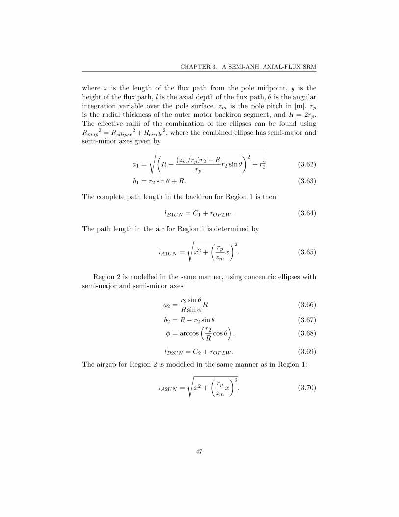
CHAPTER 3. A SEMI-ANH. AXIAL-FLUX SRM
where x is the length of the flux path from the pole midpoint, y is theheight of the flux path, l is the axial depth of the flux path, θ is the angularintegration variable over the pole surface, zm is the pole pitch in [m], rpis the radial thickness of the outer motor backiron segment, and R = 2rp.The effective radii of the combination of the ellipses can be found usingRmap
2 = Rellipse2 +Rcircle
2, where the combined ellipse has semi-major andsemi-minor axes given by
a1 =
√(R+
(zm/rp)r2 −Rrp
r2 sin θ
)2
+ r22 (3.62)
b1 = r2 sin θ +R. (3.63)
The complete path length in the backiron for Region 1 is then
lB1UN = C1 + rOPLW . (3.64)
The path length in the air for Region 1 is determined by
lA1UN =
√x2 +
(rpzm
x
)2
. (3.65)
Region 2 is modelled in the same manner, using concentric ellipses withsemi-major and semi-minor axes
a2 =r2 sin θ
R sinφR (3.66)
b2 = R− r2 sin θ (3.67)
φ = arccos(r2
Rcos θ
). (3.68)
lB2UN = C2 + rOPLW . (3.69)
The airgap for Region 2 is modelled in the same manner as in Region 1:
lA2UN =
√x2 +
(rpzm
x
)2
. (3.70)
47

CHAPTER 3. A SEMI-ANH. AXIAL-FLUX SRM
Region 3 is modelled similarly, but a partial linear segment is used tocircumvent the stator cavity
rsegment =θ
π/2
rpzm
x =θ
π/2(rp − r′). (3.71)
A circular segment follows the linear segment
Ccirc = θ
(rp +
θ
π/2(rp − r′)
). (3.72)
A final linear segment takes over past the pole face, with a length rp. Thecomplete path-length of Region 3 in the backiron is then
lB3UN = rsegment + Ccirc + rOP +(rOPLW −
rOP2
)(3.73)
and the airgap path in Region 3 is
lA3UN =
√(zmrp
(rp − r′))2
+ (r′)2. (3.74)
Region 4 is also modelling using elliptic and linear paths. The semi-major and semi-minor axes are
a4 =zm −Rzm
x+R− x (3.75)
b4 = rp + (rp − rp sin θ) . (3.76)
The path through the stator is given by
lSTAT =√
(r′)2 + (r′)2 +wSTAT
2. (3.77)
The complete path length in Region 4 through the backiron is then
lB4UN = lSTAT + C4. (3.78)
The airgap path length for Region 4 is
lA4UN =
√(zmrp
(rp − r′))2
+ (r′)2. (3.79)
48

CHAPTER 3. A SEMI-ANH. AXIAL-FLUX SRM
The unaligned leakage paths are modelled by elliptic paths across the wind-ing to the opposite pole face, where the semi-major and semi-minor axesare
al =wSTAT
2+ r′ sin θ (3.80)
bl = r′ + rOPLW . (3.81)
The inductance is then the sum of the integrated quantity determined bythe path lengths of Regions 1-4, the leakage inductance, and the permeabilityof the backiron, in a similar form to equations (3.57)-(3.59):
LtotalUN = L1UN + L2UN + L3UN + L4UN + LleakUN . (3.82)
The average torque of each design is computed via the field energy using
τavg =NsNr∆W
4π(3.83)
where Ns and Nr are the number of poles on the stator and rotor, while∆W = Waligned−Wunaligned. The energy differential ∆W is directly depen-dent on the number of windings in each pole, and on the reluctance of themotor as it moves from the minimum to maximum position. This model istherefore static, and does not account for the rotational speed of the motor.
3.3.14 Discretization of Motor Geometry for Transient Sim-ulation using Analytic Circuit Models
A dynamic model is derived which can describe transient motor performanceusing a MEC that is far simpler to implement than the static model devel-oped previously. The transient model can be normalized to agree with thestatic model, while reducing the complexity of variable airgap geometry.This is especially important in the case of the split rotor-stator AFSRM,which may experience simultaneous, independent rotations and displace-ments. The unique results for every combination of inputs are stored ina lookup table. The MEC used in this transient analysis is described bythe integral inductance function, but the backiron is ignored due to its highpermeability.
The parameters of the MEC can be derived from a simplified geometricmodel of the motor. While simple geometry typically reduces to closed-formexpressions, displacements and rotations produce complicated overlap seg-
49

CHAPTER 3. A SEMI-ANH. AXIAL-FLUX SRM
ments between the rotor and stator poles which are not easily described byclosed-form analysis. A numerical approach is therefore more appropriate.
A discrete numerical model of the motor can be generated using theoriginal geometry. The surfaces of the rotor and stator poles are discretizedin cylindrical coordinates, and overlap domains are integrated numerically.The flux path areas and lengths used by the numerical approach can beestablished directly, assuming minimal leakage. A vector-based coordinatesystem is therefore established with a rule-based filter that identifies theregions of each pole that are overlapped. The length of the flux paths thatfall within that area are then calculated for all rotational positions and alldisplacements.
The calculation performed by this technique is essentially flux path iden-tification. The primary quantities that can be drawn from the calculationare the path length and equivalent area. These values are critical to thelinear magnetic circuit model of the motor. The reluctance and inductancevalues are directly accessible with this information. The full calculation canbe seen in Appendix C. The treatment of the results from the calculationsis available at the end of the code.
3.3.15 Simplification of Motor Geometry for Transient Ther-mal Simulation using Analytic Circuit Models
A thermal model of the AFSRM may be developed using linear equivalentcircuits. A nodal structure is established which describes the location ofeach subcomponent of the motor. Nodes are connected by thermal resis-tances which represent conduction. Each node also contains a capacitiveelement which represents the heat capacity of that subcomponent. Addi-tional elements may be added to account for convection or radiation. Such acircuit model can provide dynamic thermal performance information, whichcan be combined with FEA to develop an understanding of hotspot forma-tion within motor windings.
The AFSRM model is symmetric about two axes, permitting a subsectionof the full motor to represent the complete machine. A half-segment of onepole, with structural material, is therefore modelled. Motor windings areassumed to have multiple sub-nodes, meaning that the winding is treatedas a single block of copper with dimensions equal to the thickness of theAFSRM winding. The magnitude of each thermal resistance element isaltered by the spacing of these nodes.
The elements of the thermal equivalent circuit (TEC) are described bytheir density, specific heat capacity, thermal conductivity, volume, conduc-
50

CHAPTER 3. A SEMI-ANH. AXIAL-FLUX SRM
tive path area, and node spacing. The density, specific heat capacity andthermal conductivities of the materials used in the AFSRM are shown inTable 3.4 and the volumes of each subcomponent are shown in Table 3.5,while the areas and node spacings between subcomponents and resultingthermal resistances are shown in Table 3.6. The equivalent thermal circuitfor the AFSRM is shown in Fig. D.1, Appendix D. Each resistive elementis given by using the expression
R =l
kthermA(3.84)
and each capacitive element is calculated by using the expression
C = ρV cp. (3.85)
Table 3.4: Parameters of the Thermal Model [106]
Density
Specific HeatCapacity
ThermalConductivity
ρ [kg/m3] cp [J/kgC] k [W/mC]
Backiron 7700 490 25
Casing 7850 450 52
Windings 8950 380 360
Epoxy Resin 1400 1700 0.5
Separators (7850+1400)/2 (450+1700)/2 (52+0.5)/2
Air 1.177 1005 0.0267
3.4 Optimal AFSRM Design
This section documents the implementation of the static AFSRM model forthe purpose of optimization, and examines the relationship between perfor-mance and geometry [64, 78] in the model. The wide range of achievablegeometric variations makes the AFSRM a prime example of optimal design[32, 38]. Winding configurations [78, 107], phase geometry [64], pole pitch
51

CHAPTER 3. A SEMI-ANH. AXIAL-FLUX SRM
Table 3.5: Volumes of Thermal Model Components
Component Volume, ρ [m3]
Previous Separator 3.2714e-4
Next Separator 3.2717e-4
Upper Casing 6.2832e-5
Lower Casing 1.0053e-5
Upper Winding 3.5523e-5
Lower Winding 3.6042e-5
Upper Core 6.8815e-5
Lower Core 9.6806e-5
and arc [33], flux path shape [63], phase and pole number [38] and windingcurrent waveforms [43] can all be optimized.
This section also describes alternate designs, optimization techniques,and several considerations which have impact on the optimization process.Optimization of SRMs is performed to improve both static and dynamic per-formance [36, 73, 76]. Traditional SRM optimization procedures increase theaverage torque [33] by modifying the pole pitch and arc [33], and the numberof rotor and stator poles [42]. The accuracy of both direct and indirect SRMoptimization procedures is improved by adapting AFPM optimization pro-cedures that investigate a larger number of motor parameters [32]. A directoptimization procedure uses a set of analytic design equations to define apareto-optimal set of design variations [6, 108], and an indirect optimiza-tion uses a multiobjective optimization function [33]. The pareto-optimalset is typically reduced to a smaller number of designs which describe themonotonic variation of orthogonal parameters [6]. The optimal design for aspecific application can then be selected from the reduced set.
In further discussion, the effect of important losses on the optimization ofthe AFSRM is considered, and the set of boundary conditions for the designis presented. Finally, the optimization algorithm implements the designequations developed as part of the static AFSRM model, and identifies theoptimal design.
52
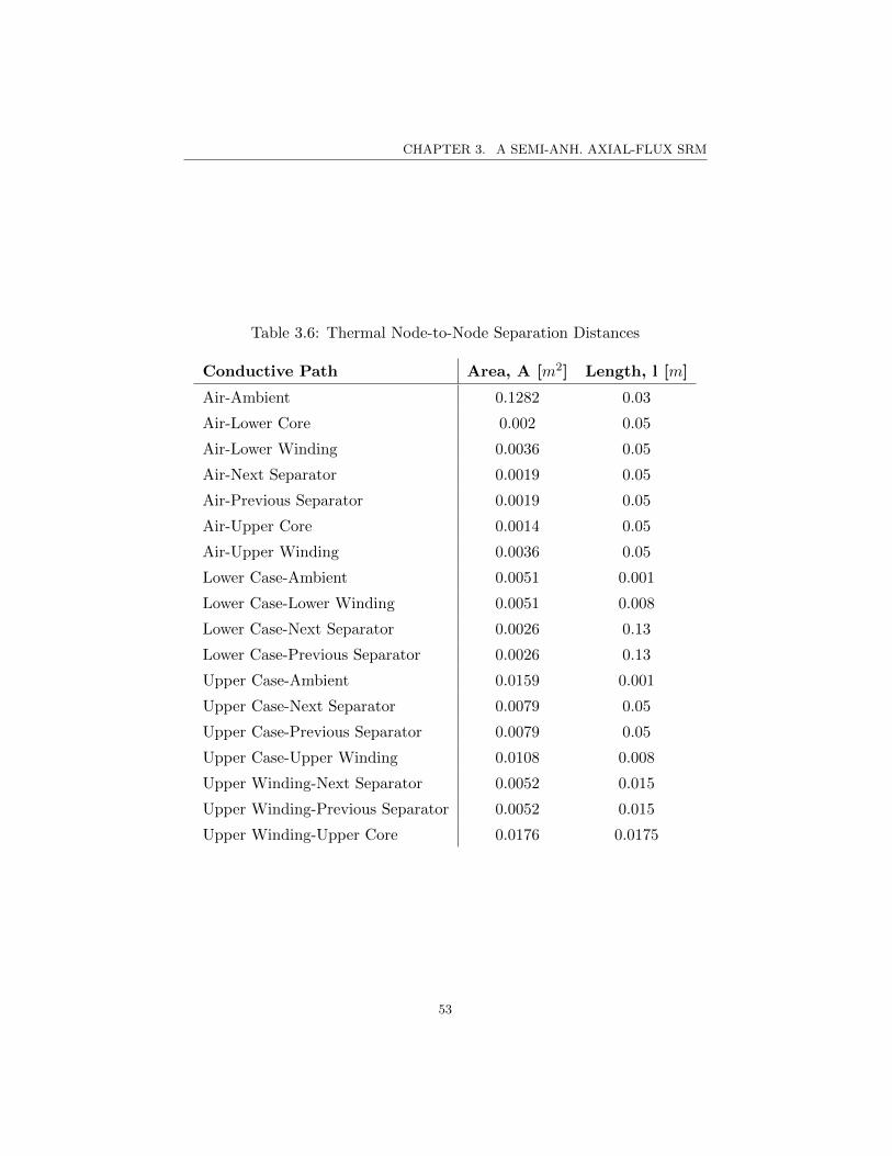
CHAPTER 3. A SEMI-ANH. AXIAL-FLUX SRM
Table 3.6: Thermal Node-to-Node Separation Distances
Conductive Path Area, A [m2] Length, l [m]
Air-Ambient 0.1282 0.03
Air-Lower Core 0.002 0.05
Air-Lower Winding 0.0036 0.05
Air-Next Separator 0.0019 0.05
Air-Previous Separator 0.0019 0.05
Air-Upper Core 0.0014 0.05
Air-Upper Winding 0.0036 0.05
Lower Case-Ambient 0.0051 0.001
Lower Case-Lower Winding 0.0051 0.008
Lower Case-Next Separator 0.0026 0.13
Lower Case-Previous Separator 0.0026 0.13
Upper Case-Ambient 0.0159 0.001
Upper Case-Next Separator 0.0079 0.05
Upper Case-Previous Separator 0.0079 0.05
Upper Case-Upper Winding 0.0108 0.008
Upper Winding-Next Separator 0.0052 0.015
Upper Winding-Previous Separator 0.0052 0.015
Upper Winding-Upper Core 0.0176 0.0175
53

CHAPTER 3. A SEMI-ANH. AXIAL-FLUX SRM
3.4.1 Optimization Techniques
Numerous techniques for optimization of machine designs exist, and areused commonly by both the industry and the research community. Eachoptimization technique has strengths and weaknesses that make it suitablefor specific problems, shown in Table 3.7.
Table 3.7: Optimization Methods
# Technique Effective Method
1. Multi-Objective Programming Multi-Variable Relative Cost Function
2. Genetic Algorithm Natural Selection
3. Bees Algorithm Random Search
4. Taguchi/Orthogonal Array Method Orthogonality of Control Parameters
5. Monotonicity Analysis Linearization of Variations in Parameters
6. FEA/Iterative Numerical Comparison Detailed Iteration for Complex Systems
7. Analytical Design Equations Simple, Continuous Optimization Surfaces
8. Iterative Analytical Comparison Simple, Discrete Optimization Surfaces
# Strengths Weaknesses
1. Complex systems, Cost, Safety Design bias, Prior knowledge
2. No analytical model necessary Slow, Can converge to local minima
3. Fast for simple systems Slow for complex systems
4. Large numbers of design variables Difficult nonlinearities, intensive computation
5. Very large numbers of design variables Does not account for local minima
6. Significant design insight Highly computationally intensive, Design bias
7. Functions in highly nonlinear systems Requires accurate system model
8. Simple implementation Computationally intensive
The goal of every optimization process is to develop a description ofthe pareto-optimal set. This set defines a boundary within which a designtradeoff is required to identify the optimal solution. All possible designswithin the boundary fulfil the optimal conditions equally. Pareto-optimalityis a condition defined by multi-objective optimization, and reduces to a singleoptimal design with only one performance variable. Suspension optimizationcontains a good example of a pareto-optimal set defined by the comfort-handling tradeoff.
3.4.2 Considerations for the Optimal Design Process
The success of the optimal design process is largely determined by themethodology behind its implementation. Several important considerations
54
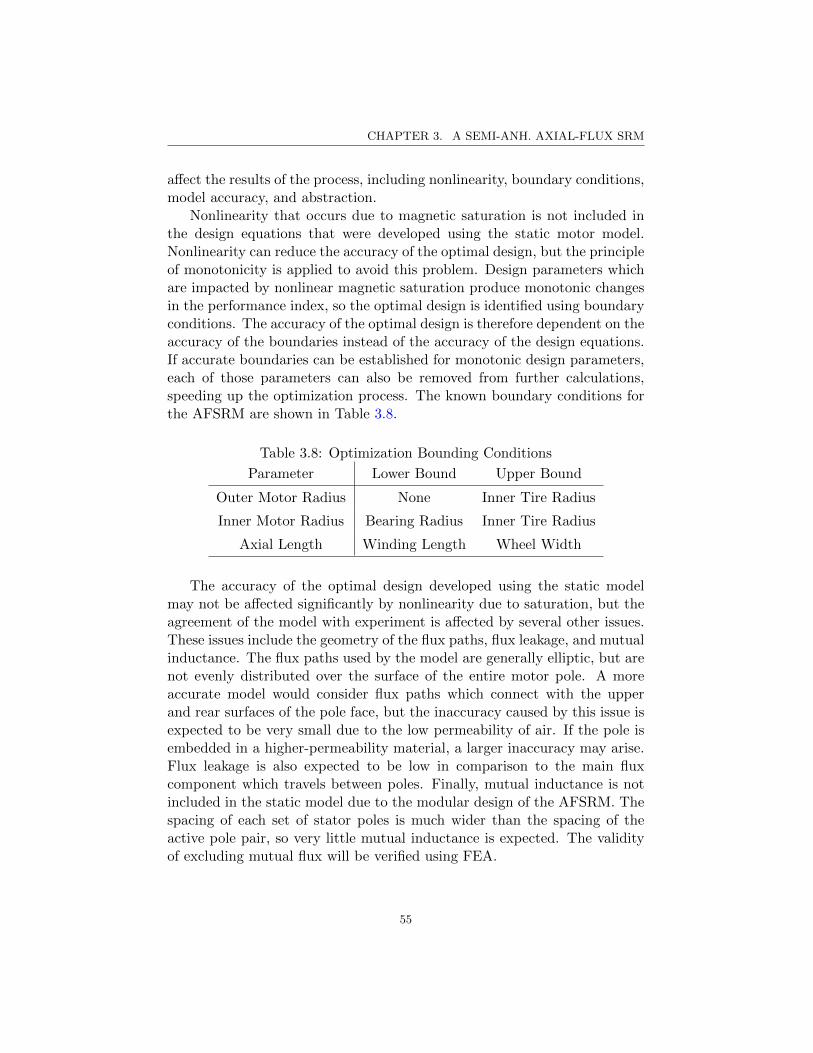
CHAPTER 3. A SEMI-ANH. AXIAL-FLUX SRM
affect the results of the process, including nonlinearity, boundary conditions,model accuracy, and abstraction.
Nonlinearity that occurs due to magnetic saturation is not included inthe design equations that were developed using the static motor model.Nonlinearity can reduce the accuracy of the optimal design, but the principleof monotonicity is applied to avoid this problem. Design parameters whichare impacted by nonlinear magnetic saturation produce monotonic changesin the performance index, so the optimal design is identified using boundaryconditions. The accuracy of the optimal design is therefore dependent on theaccuracy of the boundaries instead of the accuracy of the design equations.If accurate boundaries can be established for monotonic design parameters,each of those parameters can also be removed from further calculations,speeding up the optimization process. The known boundary conditions forthe AFSRM are shown in Table 3.8.
Table 3.8: Optimization Bounding Conditions
Parameter Lower Bound Upper Bound
Outer Motor Radius None Inner Tire Radius
Inner Motor Radius Bearing Radius Inner Tire Radius
Axial Length Winding Length Wheel Width
The accuracy of the optimal design developed using the static modelmay not be affected significantly by nonlinearity due to saturation, but theagreement of the model with experiment is affected by several other issues.These issues include the geometry of the flux paths, flux leakage, and mutualinductance. The flux paths used by the model are generally elliptic, but arenot evenly distributed over the surface of the entire motor pole. A moreaccurate model would consider flux paths which connect with the upperand rear surfaces of the pole face, but the inaccuracy caused by this issue isexpected to be very small due to the low permeability of air. If the pole isembedded in a higher-permeability material, a larger inaccuracy may arise.Flux leakage is also expected to be low in comparison to the main fluxcomponent which travels between poles. Finally, mutual inductance is notincluded in the static model due to the modular design of the AFSRM. Thespacing of each set of stator poles is much wider than the spacing of theactive pole pair, so very little mutual inductance is expected. The validityof excluding mutual flux will be verified using FEA.
55
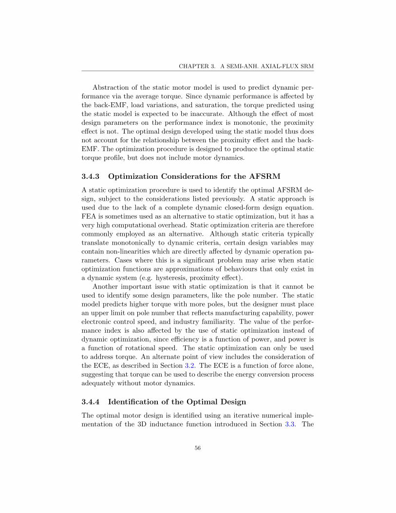
CHAPTER 3. A SEMI-ANH. AXIAL-FLUX SRM
Abstraction of the static motor model is used to predict dynamic per-formance via the average torque. Since dynamic performance is affected bythe back-EMF, load variations, and saturation, the torque predicted usingthe static model is expected to be inaccurate. Although the effect of mostdesign parameters on the performance index is monotonic, the proximityeffect is not. The optimal design developed using the static model thus doesnot account for the relationship between the proximity effect and the back-EMF. The optimization procedure is designed to produce the optimal statictorque profile, but does not include motor dynamics.
3.4.3 Optimization Considerations for the AFSRM
A static optimization procedure is used to identify the optimal AFSRM de-sign, subject to the considerations listed previously. A static approach isused due to the lack of a complete dynamic closed-form design equation.FEA is sometimes used as an alternative to static optimization, but it has avery high computational overhead. Static optimization criteria are thereforecommonly employed as an alternative. Although static criteria typicallytranslate monotonically to dynamic criteria, certain design variables maycontain non-linearities which are directly affected by dynamic operation pa-rameters. Cases where this is a significant problem may arise when staticoptimization functions are approximations of behaviours that only exist ina dynamic system (e.g. hysteresis, proximity effect).
Another important issue with static optimization is that it cannot beused to identify some design parameters, like the pole number. The staticmodel predicts higher torque with more poles, but the designer must placean upper limit on pole number that reflects manufacturing capability, powerelectronic control speed, and industry familiarity. The value of the perfor-mance index is also affected by the use of static optimization instead ofdynamic optimization, since efficiency is a function of power, and power isa function of rotational speed. The static optimization can only be usedto address torque. An alternate point of view includes the consideration ofthe ECE, as described in Section 3.2. The ECE is a function of force alone,suggesting that torque can be used to describe the energy conversion processadequately without motor dynamics.
3.4.4 Identification of the Optimal Design
The optimal motor design is identified using an iterative numerical imple-mentation of the 3D inductance function introduced in Section 3.3. The
56

CHAPTER 3. A SEMI-ANH. AXIAL-FLUX SRM
inductances of the aligned and unaligned positions are calculated, and theaverage torque is computed. There are two primary design parameters thatdrive the optimization process: the number of stator poles, and the widthof the phase windings.
The number of stator poles is selected as 8 and the number of rotor polesis selected as 6. These selections are not optimal due to the static natureof the optimization process. A dynamic optimization process is needed toevaluate the effect of increased electrical frequency due to a higher numberof poles. The 8/6 configuration is therefore used as an example. A config-uration with more poles could be chosen if the phase controller is shown tooperate at a sufficiently high frequency. More poles would produce higheraverage torque, but also greater electrical losses and a higher productioncost. Average torque for a fixed number of poles can be improved by opti-mizing the static torque profile instead.
Static optimization utilizes the integral permeance function to establishthe performance of the motor, and the loss models from Section 3.3 to es-tablish a consistent input power across designs. Power losses like mechanicaldissipative forces which effect all designs equally are ignored in the staticoptimization procedure. The procedure includes losses which do change, likeelectrical losses which are functions of the winding dimensions. The codeused for the procedure is shown in Appendix E. The final line of code definesthe ratio of the average torque to the input energy, which is used to repre-sent efficiency in the static model. The actual efficiency of the motor systemcan be calculated after the optimization process, via a dynamic simulationof motor performance where the dynamic torque curve is used to calculatepower.
3.4.5 The Optimal AFSRM Design
The optimal design exists at the maximum point on the optimization surface,represented in code by the variable T , as shown in Fig. 3.6. The efficiencycalculation using the proximity effect develops the alternate surface, repre-sented in code by motEFF , in Fig. 3.7. The two variables investigated arethe radial winding depth, and the thickness of each wire, where other motordimensions are functions of the winding depth. The arc and pitch of eachpole is determined by the number of poles, which is chosen as the common8/6 configuration.
57
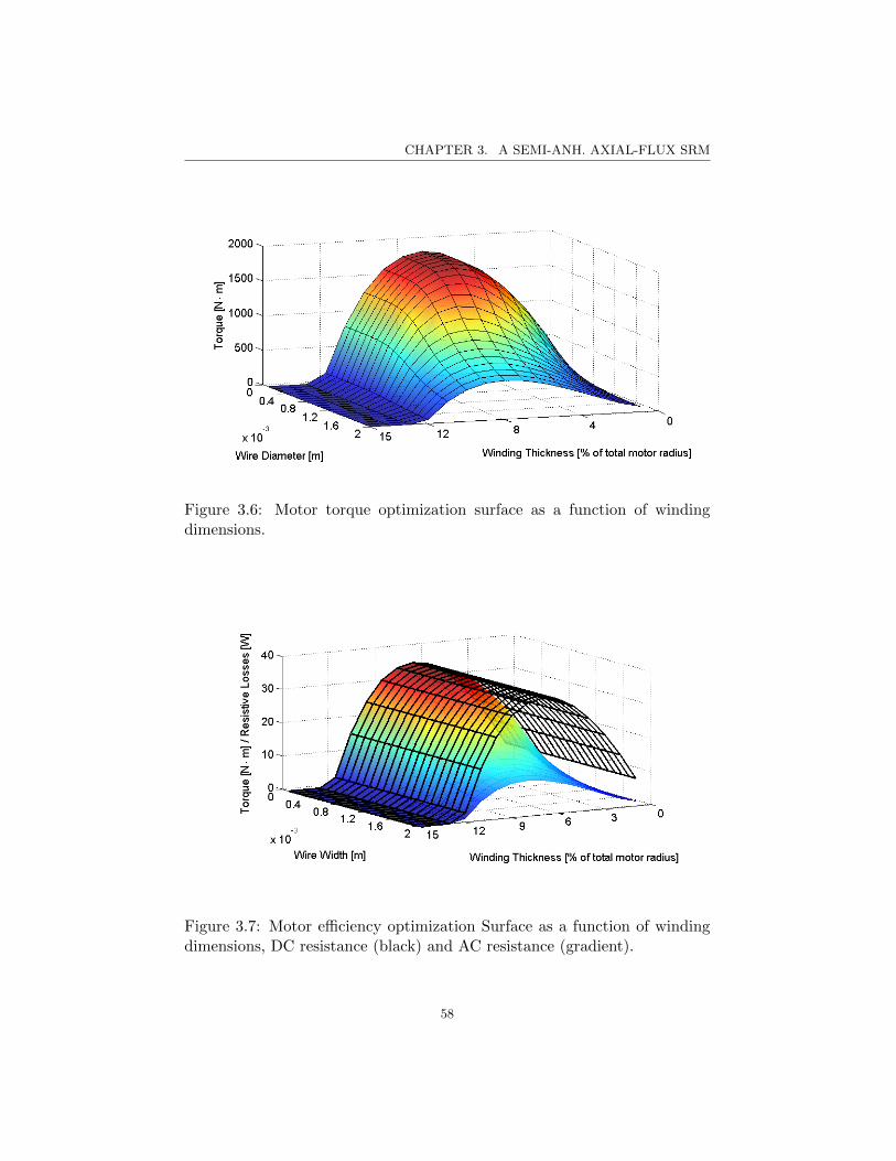
CHAPTER 3. A SEMI-ANH. AXIAL-FLUX SRM
Figure 3.6: Motor torque optimization surface as a function of windingdimensions.
Figure 3.7: Motor efficiency optimization Surface as a function of windingdimensions, DC resistance (black) and AC resistance (gradient).
58

CHAPTER 3. A SEMI-ANH. AXIAL-FLUX SRM
3.5 Control of the AFSRM
This section identifies an optimal analytic control technique which produceshigh performance at both high and low speeds. The ideal control techniqueis described in the context of several alternatives. Out of these, the optimaltechnique is selected based on its simplicity, speed, and performance. Thetechnique is then applied to the optimal AFSRM design, and optimizedusing a dynamic simulation model.
3.5.1 Control Techniques
SRM control techniques are designed to suit the pole activation sequences ofspecific designs. The activation sequence of an 8/6 SRM is shown in Fig. 3.8.The ideal control technique for the maximum power factor is theoreticallya square wave signal with maximum current over positive torque regions,and zero current over negative torque regions, but it is not realisticallyachievable. The choice between more realistic single-pole and multipoleactivation sequences will thus determine the type of current profile that thecontroller produces. Control of the current profile is achieved using switchingangles and in-phase current shaping.
Switching angles can be set statically or dynamically, but there is alwaysone value for each angle which will maximize the power factor. These opti-mal switching angles are dependent on speed, so static angles will only beoptimal at one speed. Static angles have the advantage of simplicity, butdo not maximize the performance of the controller or the motor. Dynamicswitching angles are more difficult to identify than static angles, but theycan be empirically selected based on a simulation, or analytically calculatedusing the inductance and resistance of each phase. A controller that onlyuses switching angles to influence the shape of the phase current will producea current profile similar to Fig. 3.8d.
Switching angles are used to define the width of each phase current pulse.When narrow angles produce individual current peaks separated by zero-current regions, the motor is operating in single-pulse mode, and when wideangles produce continuous current, the motor is operating in the continuous-current mode. Continuous current will increase the average torque, but canalso produce torque ripple. A motor with a larger number of phases willrequire a faster controller to achieve single-pulse control, and will be moreeasily controlled using continuous current. The speed of the controller willthus limit the number of phases in the motor, as performance is reducedwhen too much negative torque is produced. The speed of the controller
59

CHAPTER 3. A SEMI-ANH. AXIAL-FLUX SRM
Figure 3.8: Phase activation strategy for the 8/6 AFSRM during a 60 me-chanical rotation. (a) Ideal single-pulse single-pole activation, (b) Trailing-pulse multipole activation, (c) Semi-ideal multipole activation, (d) Realisticmultipole activation
60

CHAPTER 3. A SEMI-ANH. AXIAL-FLUX SRM
can be increased by increasing the phase voltage, which will also increasethe average torque.
In-phase current shaping is often referred to as instantaneous currentcontrol, and can be achieved using a range of analytical and empirical ap-proaches. The goal of current shaping is to minimize torque ripple dueto variations in the inductance profile of the active phase. The constantpower region and the speed range of the motor can be extended if torqueripple is ignored in favour of maximum torque [109], but ripple may pro-duce unwanted vibrations. Rotor inertia in the extended speed range candamp vibrations caused by torque ripple, but for stability purposes at lowspeed, ripple should be more important to the optimization criteria [110].Efficiency at high speeds is also improved by allowing torque ripple, thoughan instantaneous controller will have difficulty shaping current at high speed[110]. Accurate current shaping can be maintained if a separate controlleris used for switching angles, or if the resolution of the motor’s encoder isdecreased [111]. A robust sliding-mode controller has been designed whichwould permit current shaping at high speed [112], though a similar resultcould be given by a fuzzy controller.
The shape of the phase current in a split rotor-stator motor can also beaffected by road disturbances through the back-EMF [10]. Displacement ofthe rotor from the coaxial position alters the self-inductance of each phasedifferently [11], making the effect of road disturbances difficult to isolate.One solution has been proposed which uses a sliding-mode controller, theRMS back-EMF, and rotor displacement to reduce the impact of such roaddisturbances [113].
3.5.2 An Optimized AFSRM Control Technique
The AFSRM control strategy has two components: switching angles aredetermined analytically, and the phase current shape is managed using afuzzy controller.
Switching Angle Control
The switching angles can be analytically determined using the governingequation for the phase current, which is a function of six variables: themotor speed (ω), inductance (L), resistance (R), vertically-induced back-EMF (dL/dx), rotationally-induced back-EMF (dL/dθ), and control voltage
61

CHAPTER 3. A SEMI-ANH. AXIAL-FLUX SRM
(V ). These variables are directly apparent in the electrical phase equation:
V = IR+dλ
dt= IR+ I
dL
dt+ L
dI
dt
= IR+dL
dθ
dθ
dt+dL
dx
dx
dt+ L
dI
dt
= IR+dL
dθω +
dL
dxv + L
dI
dt. (3.86)
Re-arranging to solve for the rate of the phase current
dI
dt=
1
L
[V −
(IR+
dL
dθω +
dL
dxv
)]. (3.87)
Setting up the integral for the time interval needed to reduce the current tozero
0∫I(θ0)
L
V −(IR+ dL
dθ ω + dLdx v)dI =
toff∫t0
dt. (3.88)
Integrating, we find
− L
Rln
[V −
(IR+
dL
dθω +
dL
dxv
)]∣∣∣∣0I(θ0)
= ∆t. (3.89)
This evaluates to
L
R
(ln
[V −
(I(θ0)R+
dL
dθω +
dL
dxv
)]− ln
[V −
(dL
dθω +
dL
dxv
)])= ∆t.
(3.90)Simplifying, and using the fact that ∆θ = ∆t · ω we find
ωL
Rln
[V −
(I(θ0)R+ dL
dθ ω + dLdx v)
V −(dLdθ ω + dL
dx v) ]
= ∆θ. (3.91)
The desired switch-off angle is therefore
θoff = θf∆θ (3.92)
where θf is the angle at which the current is desired to reach zero. While(3.92) is useful to determine a dynamic switch-off angle, it does not addressthe issue of optimization. The optimal value of θf for maximum torque willdiffer from the optimal value of θf for minimum ripple. The assumption is
62

CHAPTER 3. A SEMI-ANH. AXIAL-FLUX SRM
also made in (3.92) that the motor should operate under single-pulse control.The value of θf will therefore be optimized in the same way that the optimalstatic switching angle will be determined. A dynamic switch-on angle hasyet to be defined, and will therefore also be calculated using a static tuningprocedure.
An iterative method is used to develop an optimization surface for thestatic switching angles. The angle optimization surface is shown in Fig. 3.9.The optimal static switch-off angle is chosen to be −22.5, and the switch-on angle is chosen to be 22.5, corresponding to continuous-current control.The equivalent optimization for θf is shown in Fig. 3.10, where a value of22.5 is once again found to be optimal. The dynamic torque profile withback-EMF, rotor-stator displacement, phase inductance, and DC resistance,given a constant input voltage over a range of switch-on angles is shown inFig. 3.11, and over a range of switch-off angles in Fig. 3.12.
Figure 3.9: Switching-angle tuning procedure.
Current Shaping
Current shaping is achieved using a fuzzy controller with the back-EMFand vertical displacement of the rotor as inputs, and the voltage offset asan output. The back-EMF is used to regulate the output of the controller,and to stabilize the torque profile by reducing ripple caused by vibration.The vertical displacement is used to adjust the voltage output set-pointto a value which provides optimal torque, and reduces ripple due to large
63

CHAPTER 3. A SEMI-ANH. AXIAL-FLUX SRM
Figure 3.10: Active switch-off angle tuning procedure.
Figure 3.11: Dynamic torque profiles used for switch-on angle tuning.
64
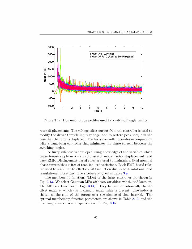
CHAPTER 3. A SEMI-ANH. AXIAL-FLUX SRM
Figure 3.12: Dynamic torque profiles used for switch-off angle tuning.
rotor displacements. The voltage offset output from the controller is used tomodify the driver throttle input voltage, and to restore peak torque in thecase that the rotor is displaced. The fuzzy controller operates in conjunctionwith a bang-bang controller that minimizes the phase current between theswitching angles.
The fuzzy rulebase is developed using knowledge of the variables whichcause torque ripple in a split rotor-stator motor: rotor displacement, andback-EMF. Displacement-based rules are used to maintain a fixed nominalphase current that is free of road-induced variations. Back-EMF-based rulesare used to stabilize the effects of AC induction due to both rotational andtranslational vibrations. The rulebase is given in Table 3.9.
The membership functions (MFs) of the fuzzy controller are shown inFig. 3.13. We select Gaussian MFs with two variables: width, and location.The MFs are tuned as in Fig. 3.14, if they behave monotonically, to theoffset index at which the maximum index value is present. The index ischosen as the sum of the torque over the simulated time interval. Theoptimal membership-function parameters are shown in Table 3.10, and theresulting phase current shape is shown in Fig. 3.15.
65

CHAPTER 3. A SEMI-ANH. AXIAL-FLUX SRM
Table 3.9: Fuzzy Rulebase
Displacement
Input Neg Zero Pos
Output Pos Zero Pos
Back-EMF
Input Neg Zero Pos
Output Pos Zero Neg
Figure 3.13: Fuzzy membership functions for the in-phase voltage controller.
66

CHAPTER 3. A SEMI-ANH. AXIAL-FLUX SRM
Figure 3.14: Membership function tuning. Offset Index ±30% of initialvalue for width (blue), ±15% of input range for location (Red).
Figure 3.15: Shape of the phase current.
67

CHAPTER 3. A SEMI-ANH. AXIAL-FLUX SRM
Table 3.10: Fuzzy Membership Functions
Set Name Location (x) Width (σ)
Input 1 Neg -0.007 0.0063
Zero 0 0.000966
Pos 0.007 0.0063
Input 2 Neg -100 42.46
Zero 0 7.864
Pos 70 29.72
Output Neg -600 254.8
Zero 0 254.8
Pos 600 254.8
3.6 Evaluation
This section presents an evaluation of the performance of the optimal AF-SRM design. The evaluation includes static, dynamic, and thermal analyses,with a discussion of thermal analysis in motors included to clarify the impor-tance of thermal design considerations. Static evaluation is performed usingFEA to identify the behaviour of the torque, radial force, and temperatureas functions of winding current, rotor displacement, and rotation. Dynamicevaluation is performed using a simulation model of a 4-phase, 8/6 SRM in-cluding electrical, magnetic, and mechanical losses developed in MATLABSimulink, and a MEC which produces lookup tables for the back-EMF inboth vertical and rotational directions. Finally, the dynamic motor torque,power, current, speed, and efficiency are calculated.
3.6.1 Dynamic Simulation Methods
Dynamic simulation methods are used to evaluate performance criteria [38]after a design has been optimized for a specific application [41, 74]. Dy-namic performance of current-controlled motors is typically evaluated us-ing Simulink [114], codes such as MRVSim [74], FEA [32, 67], or manualMATLAB codes [32]. Voltage-controlled motors have been modelled usingPSPICE [115], and simulated analytically [77]. Dynamic performance eval-uation has identified motors using hybrid current and voltage control with
68

CHAPTER 3. A SEMI-ANH. AXIAL-FLUX SRM
constant power regions as high as 12000 [rpm] [74], and machines with ef-ficiencies above 95% [42]. Dynamic evaluation is also important to identifythe shape of winding currents, the effect of both back-emf and pole geometryon torque, and in some cases the lateral stress [26].
3.6.2 Thermal Performance and Cooling
Thermal analysis is an integral component of the motor design process thatdescribes the effect of winding temperature on performance. Field windingshave increased resistivity at high temperature, which increases electricallosses and reduces performance. Thermally optimized designs improve cool-ing, and reduce the temperature of the field windings by maximizing theheat transfer coefficient at the exterior of the machine. Optimal design istypically achieved using FEA.
Modern optimal motor design involves coupled electrical, mechanical,thermal, and fluid dynamical analyses [99]. Coupled analysis [116] is use-ful to evaluate the actual operation of a machine with certain size, power,and efficiency requirements. FEA is typically used to treat problems withhighly-coupled physics in complicated geometric situations [116], while lin-ear circuit analysis can be used to reduce the computational load, or todevelop transient performance data [54, 99].
Although an analytical design procedure would allow for precise opti-mization of electric motors, thermal and fluid dynamical analyses have notbeen sufficiently generalized to permit reasonable analytic description [117].A limited understanding of fluid flow in a motor can be developed using thetheories of Taylor and Couette, but such an approach is largely restrictedto non-dimensional numerical trends [117]. Some degree of FEA is thereforepresent in many design procedures [118].
Thermal and fluid dynamical analysis is often performed separately fromelectromechanical analysis [118, 119] to reduce computational overhead, butsuch an approach does not permit inclusion of thermal effects in the opti-mization process. An alternate approach couples thermal and electrome-chanical analyses, but assumes a DC coil excitation which does not includeAC losses [99].
The thermal design of axial-flux in-wheel motors is driven by the totalpower dissipated as heat in the stator by the winding [120]. Air-cooled de-signs are preferred due to their intrinsic simplicity, where liquid cooling inhub motors leads to increased fragility [120]. Concentrated windings are like-wise preferred since they reduce the total quantity of copper needed by themotor, and subsequently reduce resistive losses in the windings [121]. Such
69

CHAPTER 3. A SEMI-ANH. AXIAL-FLUX SRM
windings can be implemented in a modular design, but structural supportof modular stator poles can be a challenge [121].
Axial-flux motor designs can vary widely in operating temperature [118,119], suggesting that cooling techniques have similarly variable success.Stead-state temperature in air-cooled machines can rise above 400[C] un-der high load, while water-cooled machines with similar loading stay below100[C] [122]. Most motors suitable for duty in EVs operate below 100[C][118], but some may reach temperatures above 200[C] [123]. The tempera-ture dependence of both resistivity and permeability can thus make coolingperformance a limiting factor in a motor design, and it is therefore critical todevelop a highly coupled analysis procedure [100]. Full FEA of all associatedphysics can be used [99], or equivalent thermal parameters can be updatedin a simpler FEA model using known lumped-parameter equations [100].
A combined lumped-parameter FEA-based thermal approach is used inthis thesis. The thermal limit of the machine is demonstrated using a nor-malized heat generation input, and a FEA-based generalized hotspot tem-perature output for the AFSRM. Such an approach can be extended to otherdesigns by FEA, and reuse of the normalized heat input. FEA is thus usedto produce both performance and thermal behaviour information.
3.6.3 Static Finite-Element Analysis of the AFSRM
This thesis utilizes COMSOL 4.3, a commercial FEA program.
Static Motor Performance for the Flat-Pole AFSRM
The motor is verified using COMSOL 4.3 and the AC/DC package in 3D.A high-density mesh is used to produce accurate results, and the torqueis calculated for a single pole. The mesh in Fig. 3.16 is applied using thebuilt-in COMSOL node-placement algorithm, and manually controlled usingthe available mesh parameters. The unaligned 3D flux pattern is shown inFig. 3.17. Torque is produced at the edge of the stator, in the region thatwould saturate for a non-linear backiron material. Two evaluations of motortorque are given, one for linear backiron permeability, and the other for themore realistic nonlinear backiron permeability determined by the BH curvefor an SLSMC.
Static Performance with Linear Permeability
The static torque profile of the optimal motor geometry with linear backironmaterial is given by Fig. 3.18. The full excitation strategy yields a periodic
70

CHAPTER 3. A SEMI-ANH. AXIAL-FLUX SRM
Figure 3.16: Comsol Model Mesh
Figure 3.17: Flux Streamlines Along the Axis
71

CHAPTER 3. A SEMI-ANH. AXIAL-FLUX SRM
static torque profile with a 60 wavelength, as shown in Fig. 3.19. Thesingle-pole static torque profile is reflected across the aligned position, tothe beginning- and end-points of the full wavelength, completing the fullmultipole excitation profile.
Figure 3.18: Static torque profile with varying winding current for linearbackiron permeability.
Static Performance with Nonlinear Permeability
The BH curve for an SLSMC, shown in Fig. 3.20, is now used to govern thebackiron permeability, given that the nonlinear backiron material will expe-rience saturation. Linear extrapolation is used on either end of the curve.The static torque profile of the optimal motor geometry with nonlinear back-iron material is then given by Fig. 3.21. The full excitation strategy for thenonlinear backiron material yields a periodic static torque profile with a 60
wavelength, as shown in Fig. 3.22. The single-pole static torque profile isreflected across the aligned position, and extrapolated to the beginning- andend-points of the full wavelength. The beginning of the static torque profileis then interpolated to the end of the reflected profile to complete the fullmultipole excitation profile.
72

CHAPTER 3. A SEMI-ANH. AXIAL-FLUX SRM
Figure 3.19: Interpolated-extrapolated multi-phase-excitation static torqueprofile for linear backiron permeability.
Figure 3.20: Sintered lamellar soft magnetic composite BH curve [124].
73

CHAPTER 3. A SEMI-ANH. AXIAL-FLUX SRM
Figure 3.21: Static torque profile with varying winding current for nonlinearbackiron permability.
Static Thermal Performance of the AFSRM
The thermal analysis procedure for the AFSRM requires the full geometryof the design to be present in the FEA model. The stator is symmetric, butthe relative positions of the rotor and stator are not, thus a single motorsegment would not reflect the thermal performance of the entire machine.The heat input to the machine is normalized to permit application to anydesign, at a fixed MMF (F ). The resulting current is given by:
I =F
N(3.93)
where N is the number of wires in the winding. The input heat density isthen:
74

CHAPTER 3. A SEMI-ANH. AXIAL-FLUX SRM
Figure 3.22: Interpolated-extrapolated multi-phase-excitation static torqueprofile for nonlinear backiron permability.
75

CHAPTER 3. A SEMI-ANH. AXIAL-FLUX SRM
P
V=
I2R
V=I2ρlWIND
AV=
F 2ρN lWINDN
N2A[lWIND · rWIND · lWINDN ]
(3.94)
=F 2ρ
NA[lWIND · rWIND](3.95)
=F 2ρ
l2WIND · r2WIND · (π(d/2)2)/d2
(3.96)
=4ρF 2
πA2WIND
(3.97)
where P is the thermal power, I is the current in the wire, ρ is the resistivityof the wire, A is the cross-sectional area of the wire, d is the diameter ofthe wire, R is the resistance of the winding, lWIND is the depth of thewinding, V is the volume of the winding, rWIND is the radial thickness ofthe winding, and AWIND is the total cross-sectional area of the winding.The normalization surface is given by Fig. 3.23.
Figure 3.23: Input heat-flux normalization surface.
The normalized heat input can be handled in several ways, includingpassive and active cooling measures. The measures used the thermal model
76

CHAPTER 3. A SEMI-ANH. AXIAL-FLUX SRM
of the AFSRM are generalized to a set of boundary conditions for passivecooling with air as a refrigerant. The actual mechanism by which heat istransferred to the refrigerant can be by convection, conduction, radiation, ora combination of all three. Heat flow will follow the path of least resistance,which for a uniform material will be linear. The linear flow will be set up tomatch the boundary conditions. Exposure of internal and external surfacesto convective environments with known heat transfer coefficients is termedthe Robin condition, while the assumption of fixed surface temperatures istermed the Dirichlet condition.
This thesis chooses the Dirichlet condition at a variable distance from theheat source. The distance from the source is a function of the effectivenessof the cooling system. If the system can maintain a constant-temperaturesurface closer to the windings, the system is more effective, and the tempera-ture of the windings will therefore be lower. More complicated fluid-dynamicanalysis is necessary to properly model the heat transfer coefficient and theconvection process at the surface of the machine.
The maximum winding temperature is given by the surface shown inFig. 3.24. The maximum temperature is well within the operating limits ofcopper wire, and significantly lower than the limits of the winding insulationand the SLSMC.
Figure 3.24: Maximum temperature in the AFSRM.
3.6.4 Dynamic Performance of the AFSRM
Dynamic performance is determined by placing the lookup tables and empir-ical relationships between each important performance parameter into the
77

CHAPTER 3. A SEMI-ANH. AXIAL-FLUX SRM
Simulink model.
Performance Parameters for the Simulink Model
The lookup tables for the back-EMF, vertical force, and inductance of themotor are shown in Figs. 3.25, 3.26, and 3.27, as developed by the MEC-type discretization technique in Section 3.3. The differential inductance inFig. 3.25 is used to calculate the back-EMF, as in (5.4). The non-normalizedvertical force in Fig. 3.26 is used to calculate the real vertical force usinga polynomial fit of the motor torque’s dependence on current. The verticalforce is directly proportional to the magnitude of the torque.
Figure 3.25: Non-normalized differential inductance used to compute theback-EMF.
The data used in the lookup table for the torque as a function of wind-ing current and rotor angle is developed using FEA in Section 3.6.3. Theempirical relationships between torque and vertical rotor displacement arepresented in Fig. 3.28 using a simplified linear approach with FEA verifica-tion.
Dynamic Performance of the AFSRM
The torque of the optimal AFSRM is given in Fig. 3.29, followed by currentin Fig. 3.30, and speed in Fig. 3.31. The efficiency of the motor systemincluding AC resistive losses and backiron hysteresis, subject only to themotor’s own inertial load, is shown in Fig. 3.32. The efficiency calculation isbased on a mechanical output and an electrical input, both of which contain
78

CHAPTER 3. A SEMI-ANH. AXIAL-FLUX SRM
Figure 3.26: Non-normalized vertical force without the effect of variablewinding current.
Figure 3.27: Motor inductance used to compute the winding current fromthe winding voltage.
79

CHAPTER 3. A SEMI-ANH. AXIAL-FLUX SRM
Figure 3.28: Vertical rotor forces due to displacement from the aligned po-sition, normalized to the linear force-displacement curve.
significant noise and are subject to a wide margin of error, though a linear fitof the data remains below unity. The performance of the motor presentedin this chapter is therefore shown to be very high, but a more detailedinvestigation of a larger system is needed to complete the evaluation of thisdesign. The motor model is thus placed in a larger vehicle model in Chapter5.
80
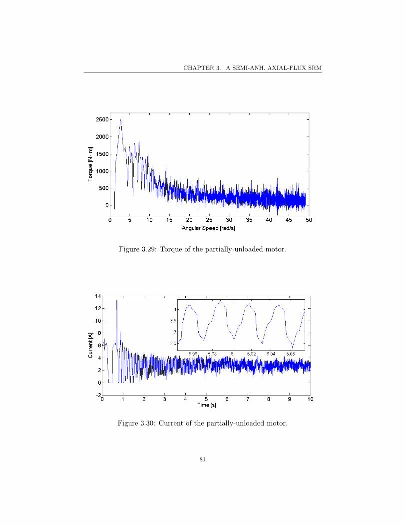
CHAPTER 3. A SEMI-ANH. AXIAL-FLUX SRM
Figure 3.29: Torque of the partially-unloaded motor.
Figure 3.30: Current of the partially-unloaded motor.
81

CHAPTER 3. A SEMI-ANH. AXIAL-FLUX SRM
Figure 3.31: Speed of the partially-unloaded motor.
Figure 3.32: Efficiency of the partially-unloaded motor.
82

Chapter 4
An Automotive HubSuspension System
4.1 Introduction
This chapter presents a novel suspension configuration for vehicles with largeunsprung masses. The suspension system is used to reduce the effect ofvibrations on vehicle handling, passenger comfort, and motor durability.The classification of vehicle vibrations is presented, and their sources aredescribed. Vibrations caused by the road surface and by the motor itselfare modelled. The result of unmitigated vibration on both passengers andvehicle systems is investigated. A half-vehicle model including the novelsuspension configuration is then developed. Finally, a control techniquewith optimized parameters is applied to the half-vehicle model, and testedusing both road- and motor-induced vibrations.
4.1.1 Context of the Suspension Design
Vehicle suspensions can be described using quarter [125], half [126], or full[127] vehicle models. Inputs to the suspension model include the longitudinalvelocity and road surface, but acceleration can be added to account forlongitudinal load transfer [126], and steering can be added to account forlateral load transfer [128, 129]. Longitudinal velocity profiles used for vehicletesting include the UDDS and HWFET drive cycles [130]. Road surfacemodels can be generated using a set of standardized functions, includingstep [131], sine [132, 133], and white noise distributions [134]. Road profilesgenerated using white noise are standardized by the ISO with a set of power-spectral densities (PSDs) for each surface [135].
Preliminary analysis of passive suspension systems can be performedusing invariant points [136] in the frequency spectrum, and the natural fre-quencies. Invariant points, however, rely on the assumption that tire damp-ing is negligible. Such assumptions can be misleading since tire damping
83

CHAPTER 4. AN AUTOMOTIVE HUB SUSPENSION SYSTEM
couples unsprung mass acceleration to the sprung mass [137], and thus hasa significant impact at the wheelhop frequency [138].
Suspension systems using passive [139], semi-active [140], and fully active[125, 141] components can be optimized to improve multiple performanceindices. Most designers focus on the ride comfort index, but some includeroad holding considerations [133, 142]. Passive suspension systems are tunedto a specific road roughness [139], while semi-active suspensions with slowresponse times can be used to adjust damping for specific surfaces [140], andsuspensions with fast response times can be used to dynamically improveperformance [13]. Dynamic performance is bounded at the theoretical up-per limit [125] defined by a fully active suspension with infinite bandwidth,where the system can both generate and dissipate energy. Suspension com-ponents with active damping ability include solenoid- and servo-valve hy-draulic [143], electro- and magneto-rheological [144, 145], piezoelectric [146],and eddy-current dampers, and linear-motor-type actuators [147, 148].
Designs have been suggested with a range of components that use linear-quadratic [148], model-predictive (MPC) [131], skyhook (SH) [149], modifiedSH [150], groundhook (GH) [151], acceleration-driven damping (ADD) [13],neural network [152], and fuzzy logic [141, 153] control to achieve improvedperformance. Control laws for active suspensions can also be used for semi-active devices in the clipped-optimal [131] configuration.
A semi-active planar suspension system is applied to the split rotor-stator in-wheel motor design in Chapter 3. The parameters of the suspen-sion system will be tuned using traditional methods, but unlike [14], theconfiguration of the system places the mass of the hub motor in series withthe mass of the wheel, reducing vibrations that are transmitted to the sta-tor of the in-wheel motor. The following sections describe vehicle vibrations,damage to electric motors caused by vibration, the modelling and controlof a suspension system which can reduce vibration damage to the in-wheelmotor, and the outcome of the testing process for that suspension.
4.1.2 Vibrations in Automotive Suspensions
Vibration in electric vehicles can be developed internally by motor operation,and externally by road roughness. Vehicle vibrations are separated into threecategories:
• Noise —Below 20 Hz
• Vibration —Above 20 Hz and Below 100 Hz
84

CHAPTER 4. AN AUTOMOTIVE HUB SUSPENSION SYSTEM
• Harshness —Above 100 Hz
All three categories of vibration can be referred to together as NVH. Thesources of NVH are shown in Table 4.1.
Table 4.1: Sources of Vibration Excited by Road Roughness and EnginePerformance [154]
Vibrations Caused by the Road Surface
Road-induced suspension disturbances are caused by road-surface irregu-larities including cracks, potholes, and the roughness of the actual roadmaterial. Road surface models can be generated using a set of standardizedfunctions, including step, ramp, sine, and white noise distributions. A realroad is typically described by a Gaussian white noise signal, but careful at-tention to the PSD of the signal is necessary to normalize its magnitude.The ISO maintains a standardized set of PSDs that can be used to generateroad models for any surface. The ISO approach is best described by [134],using the nomenclature given in Table 4.2. At a constant speed, the PSD isgiven by the expression
Gq(n) = Gq(n0)(n
n0)−w (4.1)
85

CHAPTER 4. AN AUTOMOTIVE HUB SUSPENSION SYSTEM
Table 4.2: Road Roughness Nomenclature
Parameter Description Parameter Description
Gq(n) Road PSD Gq(n0) Road roughness coeff.
n Spatial freq. n0 = 0.1 cyclem Ref. spatial freq.
Ω Spatial ang. freq. Ω0 = 2πn0 Ref. spatial ang. freq.
ω Angular velocity ω0 = 2πf Lowest cut-off ang. freq.
1.75 ≤ w ≤ 2.25 Waviness u Constant vehicle velocity
f Time frequency w(t) White noise with PSD=1
H(ω) Transfer function Sw(ω) = 1 PSD of white noise
zr(t) Road roughness
Gq(Ω) = Gq(Ω0)(Ω
Ω0)−w. (4.2)
If f = un
Gq(f) =Gq(n0)n0
2u
f2. (4.3)
then with ω = uΩ,
Gq(ω) =Gq(Ω)
u=Gq(Ω0)u
ω2. (4.4)
To avoid division by zero at ω = 0
Gq(ω) =Gq(Ω0)u
(ω2 + ω02). (4.5)
The theory of vibration states that
Gq(ω) = | H(ω) |2Sw(ω) (4.6)
which gives the transfer function to be
H(ω) =
√Gq(Ω0)u
ω0 + jω(4.7)
where under Laplace transform, H becomes
H(s) =
√Gq(Ω0)u
ω0 + s. (4.8)
86

CHAPTER 4. AN AUTOMOTIVE HUB SUSPENSION SYSTEM
This equation can be used to derive the differential form of the road rough-ness:
zr(t) + ω0zr(t) =√Gq(Ω0)uw(t). (4.9)
In a more useful form this becomes
zr(t) + 2πun0zr(t) =√Gq(Ω0)uw(t). (4.10)
As [134] proved, this equation can be used to design a Simulink diagramthat can inject a specific road roughness signal into a vehicle model throughthe tire. The frequency range of road-induced vibrations is dependent onboth the road surface and the vehicle speed, and may include the full rangeof NVH.
Vibrations Caused by Hub Motors
Internal vibration caused by motor operation occurs at frequencies which aretied to the rotational frequency of the device. The low, or possibly directgear ratio used in a hub motor translates to a low operational frequencyrange dictated by the rotational speed of the tire. The angular velocityis dependent on the size of the tire, which can vary from 14 − 17 [in] forpassenger vehicles. The Goodyear Assurance Fuelmax is a good exampleof a modern commercial tire, and will be used as a template for furtherdiscussion.
A driving vehicle moves at speeds between 0−120 [km/h] during normalduty cycles. A hub motor placed in each wheel will be required to matchthe angular velocity of the tire over this range. The overall diameter of thetire (dtot, [mm]) can be estimated using standard sidewall geometry stamps,which are recorded as ‘000/11R22’, where the first three numbers representthe section width (ls, [mm]), the second two numbers represent the aspectratio (AR), and the third set represents the interior diameter (di, [in]) ofthe tire:
2 ·AR · ls + di · 25.4 = dtot. (4.11)
The total diameter can be as low as 23.5 [in] and as high as 29.1 [in] for theFuelmax tire. At 120 [km/h], the angular velocity of the wheel is given by:
120[km/h] · 1000[m/km] · 13600 [s/hr]
π · dtot[in] · 25.4[mm/in] · 0.001[m/mm]= ω [rev/s] (4.12)
87

CHAPTER 4. AN AUTOMOTIVE HUB SUSPENSION SYSTEM
The range of angular velocities can stretch as high as 17.8 [rev/s] witha small tire to 14.4 [rev/s] with a large tire, or 111.6881 [rad/s] to90.1949 [rad/s]. The motor-induced frequency range is therefore between0 − 18 [Hz], or 0 − 144 [Hz] with consideration of 8 stator poles. Thisrange is far below the resonance zone for electric motors. Hub motors willtherefore be damaged primarily by road-induced vibration.
4.1.3 The Demand to Reduce Vibration
Passenger Discomfort and Human Resonance
Vehicle vibrations can cause a variety of discomforts in passengers, given inFig. 4.1. Avoidance of high amplitude vibrations at any frequency is there-fore desirable. The suspension system should aim to improve ride comfortwithin the handling and safety limits of the vehicle. A suspension for a hubmotor drive system should also reduce vibrations that are experienced bythe stator. These vibrations can cause significant damage and componentfailure.
Figure 4.1: Discomfort experienced by passengers due to vibration excitedby road roughness and engine performance [154].
4.1.4 Damage to Electrical Machines
There are four mechanisms through which damage can be caused to anelectric motor: Vibration Sparking, Partial Discharge, Mechanical Wear,
88

CHAPTER 4. AN AUTOMOTIVE HUB SUSPENSION SYSTEM
and REB Failure.
• Vibration Sparking occurs when parasitic currents are generated by vi-brations in magnetic systems. Small airgaps are conducive to electricalarcing, which can cause pitting in bar magnets [155].
• Partial Discharge is developed when high voltage stress is applied to adielectric material. Defects and voids within the material with a lowerrelative dielectric constant may reach the Corona Inception Voltage,thus producing sparking behaviour [156].
• Mechanical Wear can manifest as degradation of sleeve bearings, loos-ening of rotor bars, accumulation of debris in the oil guards betweenrotor and stator, changes in mounting conditions (deterioration ofgrouted base, changes in alignment/soft foot), and loosening of otherobjects mounted to the motor [157].
• REB Failure is generally a prolonged process, in which wear particlesbuild up in the lubricant, increasing viscosity and friction losses [93].Severe, immediate damage due to vibration is not common.
Suspension systems can be used to reduce motor- and road-induced vibra-tions that cause all four of these mechanisms. Avoidance of resonant frequen-cies which occur primarily between 1− 10[kHz] [158] should be emphasizedduring the design process for this reason.
4.2 Design of the In-Wheel Suspension
Since the main purpose of the suspension system is to maintain road holdingforces while minimizing transmission of vibrations from the road to thechassis, traditional suspension design relies on the trade-off between thesetwo elements. The suspension system model describes the ride comfort ofthe passengers, the road holding index, the durability of mechanisms in theunsprung mass, the wheel hop mode, and the cornering behaviour of thevehicle. The ride comfort of the passengers is measured by the frequencyresponse of the system in both displacement and acceleration domains, whilethe road holding index is calculated from the compression of the tire.
The optimization parameters are the durability, cornering behaviour,and wheel hop. Durability is a function of the damping forces between therotor and stator of the motor, and can be interpreted as the ‘ride comfort’ ofthe unsprung mass. Cornering behaviour is derived from the roll stiffness,
89

CHAPTER 4. AN AUTOMOTIVE HUB SUSPENSION SYSTEM
where increased stiffness reduces the roll rate. Wheel hop is a condition-specific problem, and is also improved with an increased effective stiffness.The combination of the stiffness and damping behaviours of the suspensionsystem determines the effect of road disturbances on the vehicle.
The semi-active suspension system identified in Section 2.3 is constrainedby the inner radius of the motor, the outer radius of the wheel bearings,and the mount needed to connect the axle to the wheel. The constraintssuggest a compact system is needed. The system is developed in a planarconfiguration next to the motor. The suspension system is not designed inthis thesis, but the stiffness and damping ratio parameters of the suspensionmodel will be investigated.
An optimal damping ratio can be determined for each road surface andvehicle speed, suggesting that a variable damping ratio is needed to traversevarying surfaces. The optimal stiffness can also be found using vehicle massand road surface parameters. An iterative approach to parameter identifi-cation for numerical simulation will therefore be applied to the suspensionmodel, as a component of the drive system developed in Chapter 3.
4.2.1 Development of the Suspension Model
A semi-active mechanical suspension system is implemented between therotor and stator of the split rotor-stator motor. Motors are placed in eachwheel of the proposed electric vehicle, resulting in four semi-independentdrive and suspension systems. A vehicle with four suspension systems maybe described by a full-car model, while two systems are described by a half-car, and a single system is described by a quarter-car.
A full-car is not used to model the in-wheel suspension system becausethe roll angle is assumed to remain small enough that it is not a large factorin the subjective ride comfort. A half-car model is chosen instead due tochassis pitch. Pitch is included in the model to account for sudden accel-eration and resulting longitudinal load transfer, which cannot be modelledusing a quarter-car. A typical half-car model is shown in Fig. 4.2.
The modified suspension model used in this section is shown in Fig. 4.3,where ff and fr represent the semi-active suspension forces. The values offf and fr are the sum of motor vertical forces and semi-active suspensioncontrol forces. The masses in the model are given by mc, which representsthe chassis, mbf , which represents the front stator, mbr, which represents therear stator, mwf , which represents the front wheel and rotor, and mwr, whichrepresents the rear wheel and rotor. A mathematical model is developedfor the modified half-car to measure suspension behaviour, using equations
90

CHAPTER 4. AN AUTOMOTIVE HUB SUSPENSION SYSTEM
Figure 4.2: Standard half-car suspension model [126].
(4.13), (4.14), (4.15), (4.16), (4.17), (4.18), (4.19), (4.22), and (4.23). Thevertical motion of the chassis is described by
mcyc − kcf (ycf − ybf )− ccf (ycf − ybf )
− kcr(ycr − ybr)− ccr(ycr − ybr) = 0 (4.13)
and the pitch motion of the chassis is described by
Icθ + df [kcf (ycf − ybf ) + ccf (ycf − ybf )]
− dr[kcr(ycr − ybr) + ccr(ycr − ybr)] = 0. (4.14)
The motion of the front stator mass is then given by
mbf ybf − kcf (ycf − ybf )− ccf (ycf − ybf )− kbf (ybf − ywf )− ff = 0 (4.15)
where ff = cbf (ybf − ywf )+ffm and the motion of the front rotor and wheelmass is given by
mwf ywf − kwf (ywf − y0f )− kbf (ybf − ywf )− ff = 0. (4.16)
91

CHAPTER 4. AN AUTOMOTIVE HUB SUSPENSION SYSTEM
Figure 4.3: Modified half-car suspension model.
92

CHAPTER 4. AN AUTOMOTIVE HUB SUSPENSION SYSTEM
Then the motion of the rear stator mass becomes
mbrybr − kcr(ycr − ybr)− ccr(ycr − ybr)− kbr(ybr − ywr)− fr = 0 (4.17)
where fr = cbr(ybr − ywr) + frm and the motion of the rear rotor and wheelmass becomes
mwrywr − kwr(ywr − y0r)− kbr(ybr − ywr)− fr = 0. (4.18)
To decouple the pitch motion term, reduction of θ to its component ycf andycr terms is necessary:
ycf = yc − dfθ (4.19)
ycr = yc + drθ (4.20)
θ =ycr − ycfdf + dr
. (4.21)
Substituting into equations 4.13 and 4.14 we obtain
ycf −
(1
mc+d2f
Ic
)[kcf (ycf − ybf ) + ccf (ycf − ybf )]
−(
1
mc+dfdrIc
)[kcr(ycr − ybr) + ccr(ycr − ybr)] = 0 (4.22)
ycr −(
1
mc+dfdrIc
)[kcf (ycf − ybf ) + ccf (ycf − ybf )]
−(
1
mc+df
2
Ic
)[kcr(ycr − ybr) + ccr(ycr − ybr)] = 0. (4.23)
These final equations encapsulate both the pitch and vertical motions of thefront and rear of the vehicle, where pitch arises from the relative motionof the two axles. The system can also be simplified using the state-spacerepresentation, where the pitch equations (4.22) and (4.23) couple two iden-tical state-space equations that describe the motion of the front and rearsuspensions. Each suspension is then described by
ddt
yc − ybyc
yb − ywyb
yw − y0
yw
=
0 1 0 −1 0 0
− kcmc
− ccmc
0 ccmc
0 0
0 0 0 1 0 −1kcmb
ccmb
− kbmb
− ccmb
0 0
0 0 0 0 0 1
0 0 kbmw
0 − kwmw
− cwmw
yc − ybyc
yb − ywyb
yw − y0
yw
+
0001mb0− 1mw
f+
0000−1cwmw
y0 .
93

CHAPTER 4. AN AUTOMOTIVE HUB SUSPENSION SYSTEM
Each state-space model describes a single 3DOF quarter-car suspension sys-tem. An equivalent 2DOF state-space model of the typical half-car can bedefined for the purpose of comparison to the 3DOF suspension system. The2DOF model is described by
ddt
yw − y0
ywyc − ywyc
=
0 1 0 0
− kcmw
(−cc+cw)mw
kcmw
ccmw
0 −1 0 1
0 ccmc
− kcmc
− ccmc
yw − y0
ywyc − ywyc
+
0− 1mw01mc
f +
−1cwmw00
y0.
A direct static comparison between the 2DOF and 3DOF suspension systemsis made using the equivalent passive transfer functions of both semi-activesystems, as in Fig. 4.4. A dynamic comparison is achieved by adding the2DOF and 3DOF suspensions to the Simulink model of the drive system,shown in Fig. F.5, Appendix F. The road surface input to the rear suspen-sion system is modified using a speed-dependent delay parameter to imitatea real vehicle. Infinite delay near zero longitudinal velocity is avoided usinga saturation condition with a maximum delay of 100 [s].
Figure 4.4: Equivalent passive transfer functions of the 2DOF and 3DOFsuspension systems.
4.2.2 Parameter Identification
The value of each parameter in the suspension model is chosen to agreewith [126], as in Table 4.3. The stiffness and damping ratio of the in-wheelsuspension system are then selected. The stiffness should be sufficient tosupport the mass of the vehicle during operation. The Lift Sufficiency Ratio
94

CHAPTER 4. AN AUTOMOTIVE HUB SUSPENSION SYSTEM
(LSR) is defined as the fraction of time during operation that the suspensionforce is sufficient to resist the inertial force experienced by the vehicle. Theratio can be defined using either the mass of the chassis or the mass of thestator. The chassis version is defined by
Table 4.3: Suspension Model Parameters
Parameter Value
Chassis Suspension Stiffness 17000 [N/m]
Chassis Suspension Damping 400 [N · s/m]
In-Wheel Suspension Stiffness 80000 [N/m]
Tire Stiffness 200000 [N/m]
Tire Damping 200 [N · s/m]
Chassis Mass 690 [N · s/m]
Chassis Moment of Inertia 1222 [kg/m2]
Centre-of-Mass to Front 1.3 [m]
Centre-of-Mass to Rear 1.5 [m]
Stator Mass 15 [kg]
Rotor Mass 15 [kg]
LSRc(kb) =1
T
T∫0
dt if
mcyckb(yb − yw)
> 1,
0 ifmcyc
kb(yb − yw)≤ 1.
(4.24)
where T is the total simulation time, mc is the mass of the chassis, yc is theacceleration of the chassis, yb is the position of the bearing and the stator,kb is the stiffness of the in-wheel suspension, and yw is the position of thewheel and the rotor. The unsprung mass version is defined by
LSRb(kb) =1
T
T∫0
dt if
mbybkb(yb − yw)
> 1,
0 ifmbyb
kb(yb − yw)≤ 1.
(4.25)
95

CHAPTER 4. AN AUTOMOTIVE HUB SUSPENSION SYSTEM
where mb is the mass of the bearing and the stator, and yb is the accelerationof the bearing and the stator. Both LSRs are shown in Fig. 4.5. A stiffnessof 80000 [N/m] is selected as the lowest value which has an LSR close to 1.The damping ratio will be selected as part of the optimization process forthe semi-active controller.
Figure 4.5: Stiffness Selection using the Lift Sufficiency Ratio and the Tran-sient Inertial Force.
4.3 Semi-Active Suspension Control
Non-linear control theory can be summarized in seven main concepts, de-scribed in Table 4.4. Each concept can be used independently, on in con-junction with any of the others to form a hybrid controller. Due to the smalltime-scales, and highly non-linear behaviour present in the model simula-tion, approximation methods are not useful to consider. Graphical andanalytical control techniques are also difficult to apply to a system whichdoes not have a direct closed-form solution, though its dynamic equationsare well described.
Adaptive control uses a set of criteria and on-line parameter estimationto ensure stability. By adjusting plant parameters, the behaviour of thesystem can be altered. In an entirely non-linear application, adaptive controlinfers results based on measurements of the system output. The bearing
96

CHAPTER 4. AN AUTOMOTIVE HUB SUSPENSION SYSTEM
Table 4.4: Nonlinear Control Concepts
Method Limitations
Describing Function Approximation Method
Phase-Plane Method Precise Method, Graphical,
Limited to 1st and 2nd order systems
Lyapunov Approach Must have a Lyapunov Function
Popov’s Method Similar to Lyapunov
Feedback Exact Linearization Linearize feedback, cancel non-linearity
Adaptive Control Requires dynamic model
Neural Networks Requires desired output or
and Fuzzy Logic expert knowledge of the system
model output parameters contain several local minima, however, makingidentification of a simple descent from the current plant to the optimal onechallenging.
Neural networks are simple learning algorithms that can map a plant’sparameters to a specified output function. When simplified inputs are se-lected to perturb the bearing, an optimal output can be identified for thecontroller. When the input changes faster than the settling time of the con-trolled system, or when any information is lost during transmission to thebearing’s upper race, selection of the optimal output is likely impossible.Techniques may be applied to converge to an acceptable solution, but theyare not generally robust.
Fuzzy logic is often applied to non-linear systems when other methodsfail. A fuzzy controller can be formulated with a minimal level of sys-tem knowledge. The rule-base of such a controller uses if-then logic, intandem with numerical rule-weights which exist in the set of optimizationvariables. Input ranges are often pre-defined by mechanical limits, leavingthe remaining optimization parameters to be the shapes and locations of themembership functions themselves.
Analytical semi-active suspension techniques include SH, GH,acceleration-driven damping, power-driven damping (PDD), and model-predictive control (MPC). Hybrid control techniques using multiple con-trol laws are also possible. Skyhook- and Groundhook-type suspensions are
97

CHAPTER 4. AN AUTOMOTIVE HUB SUSPENSION SYSTEM
compared in Table 4.5, while hybrid techniques are compared in Fig. 4.6.
Table 4.5: Skyhook and Groundhook Suspensions
System Purpose Configuration Applicability
Skyhook Comfort Chassis Damping Theoretical
Modified Skyhook Compromise Full Semi-active Realistic
Groundhook Durability Wheel Damping Theoretical
Hybrid Sky/Ground Compromise Full Semi-active Realistic
Passive - Passive Realistic
A single-sensor hybrid of the SH and ADD approaches is adopted in thissection, due to its advantageous combination of simplicity and performance.The control law [13] is given by
cb = cmax if z2 − α2x2 ≤ 0,
cb = cmin if z2 − α2x2 > 0.(4.26)
where cb is the internal suspension damping coefficient in [Ns/m].
4.3.1 Control Optimization
An iterative tuning procedure for the rotor-stator damping parameter cmaxand the frequency range selector α is shown in Fig. 4.8 over a range 0 ≤cmax ≤ 1600 and 0 ≤ α ≤ 90, where the values cmax = 1600 and α = 90 areoptimal. The road surface shown in Fig. 4.7 is used as an input.
4.4 Evaluation of the In-Wheel Suspension Sys-tem
The success of the in-wheel suspension system can be evaluated using theacceleration of the masses in the vehicle, compared to a standard half-carsuspension. The acceleration of the chassis is used to evaluate ride comfort,while the acceleration of the unsprung mass is used to evaluate the durabilityof the in-wheel drive system.
The power spectrum of the acceleration for each mass, due to the roadsurface shown in Fig. 4.7, is shown in Fig. 4.9, and the power spectrum forthe unsprung mass at several frequencies surrounding the natural frequency
98

CHAPTER 4. AN AUTOMOTIVE HUB SUSPENSION SYSTEM
Figure 4.6: Hybrid suspension control techniques [13].
99
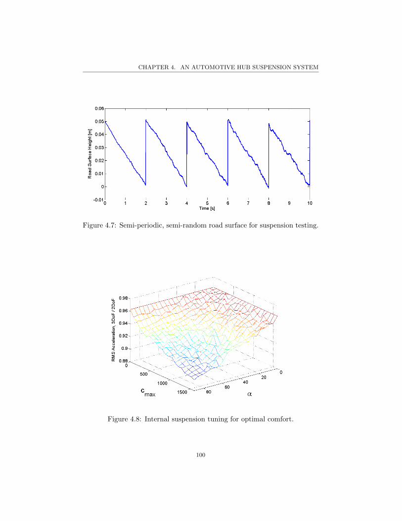
CHAPTER 4. AN AUTOMOTIVE HUB SUSPENSION SYSTEM
Figure 4.7: Semi-periodic, semi-random road surface for suspension testing.
Figure 4.8: Internal suspension tuning for optimal comfort.
100

CHAPTER 4. AN AUTOMOTIVE HUB SUSPENSION SYSTEM
is shown in Fig. 4.10. The power spectrum is a normalized representationof the magnitude of the frequency components in the vibration of the massabove the bearing. The 3DOF suspension with the semi-active controllerdoes not have the peak between 5 − 15 [Hz] normally associated with thenatural frequency. The spectrum peak is typically the primary vibrationmode that contributes to damage.
Figure 4.9: Tuned-suspension power spectrum from the semi-periodic, semi-random road surface.
Figure 4.10: Unsprung mass power spectrum at several road disturbancefrequencies.
101

CHAPTER 4. AN AUTOMOTIVE HUB SUSPENSION SYSTEM
Wheel hop occurs at the wheel hop frequency during significant distur-bances, and is generally not a large concern in automobile safety. The in-creased unsprung mass of a hub motor increases the magnitude and durationof wheel hop regardless. The effect of disturbances with small magnitudeis decreased, but the time taken to restore tire contact with the road is in-creased. Wheel hop is therefore only important to handling when contactwith the road is lost. A conditional statement can thus be implemented toutilize vertical motor forces to restore contact in emergency situations. Thecontact forces are shown in Fig. 4.11, where values above 0 represent lossof contact. The travel of the in-wheel suspension is likewise shown in Fig.4.12. The 3DOF suspension system does not exhibit wheelhop, though itdoes experience reduced contact force. The impact of the 3DOF and 2DOFsuspensions on handling can now be investigated.
Figure 4.11: Contact forces at the road surface for the 3DOF and 2DOFsuspension models.
102

CHAPTER 4. AN AUTOMOTIVE HUB SUSPENSION SYSTEM
Figure 4.12: Travel limits for the in-wheel suspension.
103

Chapter 5
Evaluation of the In-WheelDrive System
5.1 Introduction
This chapter evaluates the performance, comfort, and handling of the com-plete in-wheel drive system using coupled AFSRM, in-wheel suspension, andhalf-car handling models in Simulink. The complete system is described us-ing both static and dynamic analysis, with inclusion of electric, magnetic,and systemic factors. Electric and magnetic factors cause the majority ofthe dynamic effects in the drive system, while systemic factors define theboundary conditions for each of the evaluated criteria. These criteria in-clude acceleration, gradability, comfort, handling, and efficiency, of whichhandling is the limiting factor on safety. The major safety considerationfor an in-wheel-drive vehicle is wheel hop. Wheel hop can cause unstablehandling in two major ways: by increasing oversteer, and by interfering insteering response. A complete handling model is necessary to investigatesteering, and the variation of steering response with an increased unsprungmass. The vehicle path, yaw, and road holding can be drawn from such amodel, and can all be used to examine the effect of wheel hop on safety.
Previous studies on the handling and safety of vehicles with increasedunsprung mass have been performed both experimentally and empirically[12, 28, 59, 159]. Empirical studies have shown that the ‘feel’ of impacts tothe suspension, the pitch of the chassis, the yaw stability, and the steeringbehaviour are worse in vehicles with large unsprung masses [59]. The reduc-tion in comfort and handling is, however, less than the reduction caused byin increase in road surface roughness [59]. One cause of reduced handlingis suggested to be the overlap of the wheel hop frequency with the dampednatural frequency of the suspension [12]. The major application of thesehandling and safety studies has been the Protean in-wheel motor, a BLDCmachine weighing 31 kg. The Protean motor requires rare-earth magnetsto achieve a high enough torque density to fit inside a wheel well. The mo-tor can be used as a stand-alone drive system, or to assist an engine using
104

CHAPTER 5. EVAL. OF THE IN-WHEEL DRIVE SYSTEM
the through-the-road hybrid configuration. The handling performance of a30 [kg] hub motor will therefore be compared to that of the 30 [kg] splitrotor-stator hub motor developed in Chapter 3. The single 30 [kg] motoris placed in the wheel of the traditional half-car suspension model usingtwo coupled 2DOF suspension systems, while the split rotor-stator motoris placed in the wheel of the modified half-car suspension model using twocoupled 3DOF suspension systems. Each motor-suspension pair is placed inits own vehicle handling model. The handling model can thus be used toevaluate the combined performance of the motor and suspension systems inthe context of a vehicle.
The following sections provide a detailed investigation of the perfor-mance, comfort, and handling of the in-wheel drive system using coupledSimulink models. The inputs and outputs of each model subsystem are de-scribed in Section 5.2. The motor, suspension, and handling subsystemsare then presented in Sections 5.3, 5.4, and 5.5, respectively. Finally, theresults from the complete simulation of the in-wheel drive system includingeach subsystem are delivered in Section 5.6, along with a comparison anddiscussion of those results.
5.2 Configuration of the Simulation System
This section describes the inputs and outputs of each subsystem as theyrelate to the complete in-wheel-drive vehicle model, which is composed ofthree mechanical components. The first component is the electric motor,which supplies torque and moves the vehicle. The second component is thesuspension system, which interacts with the road and the motor to achievea safe, comfortable ride. The third component is the handling subsystem,which includes tires, steering, and safety mechanisms. Improvements tothe motor and suspension are measured using indices from the handingsubsystem.
A single motor model is simulated to standardize the behaviour of thedrive system. Two suspension models are included to contrast the effectsof modifications to the mechanical configuration of the suspension system.Two handling models are simulated in order to identify the impact of wheelhop on the handling characteristics of the vehicle. The complete modelincluding all five systems is shown in Fig. 5.1.
The inputs to the model are the desired vehicle speed and the given roadsurface. The road surface can also be broken into incline and roughness. Thevehicle speed is input to the model via a speed controller, which delivers a
105

CHAPTER 5. EVAL. OF THE IN-WHEEL DRIVE SYSTEM
Figure 5.1: Simulink diagram containing the vehicle subsystems, includingthe motor and suspension.
106

CHAPTER 5. EVAL. OF THE IN-WHEEL DRIVE SYSTEM
voltage output to the motor. The roughness is input to the model as apower spectral density, which is used to calculate the actual road surfaceanalytically as a random Gaussian noise signal. The incline is the onlydirect mechanical input to the model, and is delivered to the motor via anincreased loading condition.
The outputs of the model are the road holding index, vehicle path, motorperformance, ride comfort, and efficiency of the vehicle system. The roadholding index is evaluated using the variability in the contact force betweenthe tire and the road. The vehicle path is given by the handling model,just as the performance is given by the motor model. The ride comfort isthen calculated from the frequency response of the suspension system, andthe efficiency is determined by the total mechanical power delivered as afraction of the total electrical power used. The outputs of every subsysteminside the model are then used as the inputs to other subsystems, as shownin Table 5.1.
Table 5.1: Inputs and Outputs of the Vehicle Model Subsystems
107

CHAPTER 5. EVAL. OF THE IN-WHEEL DRIVE SYSTEM
5.3 Configuration of the Motor Simulation
The simulation model of the motor is composed of four phases, each of whichoperates on a 60 mechanical period. The active mechanical angle for eachpole is calculated from:
θs = 2π/(2Ns) = θr (5.1)
θra = (2π − θrNr)/Nr = 2π/Nr − θr (5.2)
θactive = θra − θs (5.3)
where θs is the stator pole angle, Ns is the stator pole number, θr is therotor pole angle, Nr is the rotor pole number, θra is the rotor pole arc, andθactive is the active mechanical angle. It is important to note that the rotorpole pitch is set to be equal to the stator pole pitch in order to maximizealigned inductance.
The active angle for an 8/6 single-phase activated SRM is therefore 15
when the stator and rotor pole pitches are 22.5. Multiphase activationwill extend the active angle depending on the controller. The governingequation for the phase current is a function of six variables: the motor speed(ω), inductance (L), resistance (R), vertically-induced back-EMF (dL/dx),rotationally-induced back-EMF (dL/dθ), and control voltage (V ). Thesevariables are directly apparent in the electrical phase equation:
V = IR+dλ
dt= IR+ I
dL
dt+ L
di
dt
= IR+dL
dθ
dθ
dt+dL
dx
dx
dt+ L
di
dt
= IR+dL
dθω +
dL
dxv + L
di
dt. (5.4)
A simulation can implement this equation to calculate the phase current byre-arranging:
dI
dt=
1
L
[V −
(IR+
dL
dθω +
dL
dxv
)]. (5.5)
The lookup tables used to generate the back-EMF, vertical force, and induc-tance of the motor are shown in Figs. 3.25, 3.26, and 3.27. The differentialinductance in Fig. 3.25 is used to calculate the back-EMF, as in (5.4). Thenon-normalized vertical force in Fig. 3.26 is used to calculate the real verti-cal force using a polynomial fit of the motor torque’s dependence on current.The vertical force is directly proportional to the magnitude of the torque.
108

CHAPTER 5. EVAL. OF THE IN-WHEEL DRIVE SYSTEM
The output rotational speed of the motor is translated to the longitudinalspeed of the vehicle through the tire slip condition.
5.3.1 Reduction of Longitudinal Velocity due to Tire Slip
Compression of a traditional pneumatic tire causes the effective radius ofthe wheel to decrease. A lower effective radius produces a lower longitu-dinal vehicle velocity for any given rotational frequency. Higher rotationalfrequencies generate a higher back-EMF, increased eddy current, and morehysteresis losses. A compressed tire also makes contact with the road inan elliptic patch, which produces the rolling resistance force. Rolling resis-tance creates a permanent resistive force at the radius of the contact patch.Tire compression is therefore the cause of two different losses. The rollingresistance force can be described by a lumped-parameter equation:
FRR = CRRMsprungg (5.6)
where CRR is the rolling-resistance coefficient, and g is the acceleration ofgravity. The coefficient is on the order of 10−2.
The radius of the contact patch can be computed using the mass of thevehicle. The compression caused by the sprung vehicle mass (Msprung) canbe described by an effective stiffness (ktire). The sprung force on each tireis then
Fsprung =1
4ktireδ (5.7)
where δ is the radial compression length, and a car with four tires is assumed.The radius of the ellipse (a) can then be found using
a =√R2tire − (Rtire − δ)2 =
√2Rtireδ − δ2 ≈
√2Rtireδ (5.8)
where Rtire is the actual radius of the wheel. Since δ is very small, thesquared term is removed, which simplifies the simulation by eliminating thepossibility of a negative value inside the square root. The angle throughwhich the motor rotates as the tire passes over the contact patch is given by
φ = arcsin a/Rtire. (5.9)
The effective radius can be derived as the radius at which a rotation of angleφ produces motion through an arc length equal to a:
reff =a
φ. (5.10)
109

CHAPTER 5. EVAL. OF THE IN-WHEEL DRIVE SYSTEM
The equivalent longitudinal speed of the vehicle due to tire compression,also known as slip, is given by
vvehicle = reffωmotor (5.11)
where ωmotor is the angular velocity of the rotor. The velocity of the vehicleinfluences handling, and also determined the speed at which road distur-bances are delivered to the suspension system.
5.4 Configuration of the Suspension Simulation
The suspension system is implemented in Chapter 4.1. The vehicle speedand road roughness inputs are delivered to the 2DOF and 3DOF suspensionmodels in an identical manner. The vertical motor forces are input to the3DOF suspension system between the masses of the stator and rotor. Theroad contact forces for the 2DOF and 3DOF suspensions are then input toindependent vehicle handling models.
5.5 Configuration of the Handling Simulation
A traditional passenger vehicle handling model is adapted in this section toinclude the effect of increased unsprung mass on road holding and cornering,due the presence of an in-wheel motor. The steering angle and longitudinalspeed are input to the model, which then outputs the vehicle path, yawrate, roll angle and rate, lateral velocity and acceleration, and tire sideslip.The model accounts for scrub-by-roll, camber-by-roll, steer-by-roll, the sus-pension damping and stiffness, roll damping and stiffness, and an anti-rollbar. The lateral and longitudinal load transfer, self-aligning moment, androll axis variations due to load transfer are ignored.
Each of the ignored parameters has a justification. Lateral load transferis removed from the model because hub-driven vehicles have a lower sprungmass, and therefore a smaller roll rate than a vehicle with an engine mountedon the chassis. During extreme turning maneuvers with significant lateralload transfer, the compression of the outer suspension will also ensure thatthe outer tires maintain road holding. Longitudinal load transfer is excludedfrom the model because it is seen primarily by passenger vehicles at lowspeeds, or during transitions from high speeds to low speeds or vice versa.Wheel hop at low speeds is not noticeable since the displacement from thetire’s lift point to the return point will be very small. The impulse of a given
110

CHAPTER 5. EVAL. OF THE IN-WHEEL DRIVE SYSTEM
bump at low speed will also be significantly lower than the impulse of thebump at high speed. The increased unsprung mass of a hub motor will thussee less lift than the tire of a vehicle without such motors. The roll axiscan therefore be fixed as parallel to the road surface given the exclusion ofload transfer, and the equivalent assumption that pitch and roll angles willbe small. The final exclusion of the tire’s self-aligning moment is justifiedby the mass of the in-wheel motor, which will reduce the tendency to self-alignment given a high moment of inertia. Responsive handling with sucha high moment of inertia can be achieved with an electronically-controlledsteering system.
Critical handling situations will occur primarily at high or mediumspeeds during cornering maneuvers, where the effects of a hub motor onlow speed handling have been presumed to be minimal. Wheel hop is theprimary mechanism by which the increased unsprung mass of a hub-motor-driven vehicle will impact handling. The effect of wheel hop will be a lossof traction in an affected tire. Each axle may lose traction independentlyof the other, as the road surface will reach the front tires before the reartires. The single-track half-car model used for the suspension system will,however, restrict the handling model to a single track. This means that theleft and right wheels must respond to the road surface simultaneously. Suchan assumption is valid in situations where bumps or obstacles are symmetricalong the width of the road surface.
Four traction conditions are possible in a single-track handling model:full contact by all tires, loss by the front tires, loss by the rear tires, andtotal loss by all tires. These conditions are characterized by the sign of thecontact force exerted on the front and rear sets of tires. Forces greater thanzero correspond to traction, and less than or equal to zero imply loss ornear-loss of traction. Each condition can be assigned a value of 0 or 1, andused to define the instantaneous version of the handling model.
5.5.1 The Vehicle Handling Model
Handling is a nonlinear function of vehicle velocity, road surface slope, roadholding index, and steering angle. A simplified ‘bicycle model’ uses a lin-earized treatment of handling which disregards the effect of roll. A meoreaccurate 3DOF linearized handling model includes roll dynamics [160, 161],and will be used here in the Society of Automotive Engineers (SAE) coor-dinate system with z defined along the vertical direction, y defined alongthe transverse direction, and x defined along the longitudinal direction. Thehorizontal force on each tire is the primary quantity which is linearized by
111
CHAPTER 5. EVAL. OF THE IN-WHEEL DRIVE SYSTEM
the 3DOF handling model, where the alternative nonlinear Magic Tire for-mula [162] is unnecessarily complex for this purpose. The linearized form ofthe horizontal force due to the tire slip angle is given by
Fy = Cαα (5.12)
where Cα is the cornering stiffness, and α is the slip angle. The 3DOF modelalso incorporates scrub-by-roll, camber-by-roll, and steer-by-roll. Scrub-by-roll is a linearized function of roll velocity, whereby the wheel scrub velocityis
V ′ = Kscbrφ (5.13)
where Kscbr is the scrub-by-roll coefficient, and φ is the roll velocity. Thevelocity of the wheel motion relative to the surface is then
vN = V + a′r + V ′ (5.14)
where vn is the lateral wheel velocity, V is the lateral vehicle velocity, V ′
is the lateral velocity of the wheel relative to the vehicle, and a′r is therotational yaw velocity around the vehicle’s vertical axis, given a′ is thedistance to the wheel from the axis. The slip angle is defined as
α = δ − vNuN
(5.15)
where δ is the steering angle of the driver, uN is the forward vehicle velocity,and vN is the horizontal vehicle velocity. Arranging terms in the previousequation,
Fy = Cα
(δ − V + a′r +Kscbrφ
uN
). (5.16)
Camber-by roll is a linear function of camber angle. The camber force is
Fγ = Cγγ (5.17)
where Cγ is the camber stiffness, and γ is the camber angle. The camberangle is
γ = Kcbrφ (5.18)
whereKcbr is the camber-by-roll coefficient, and φ is the roll angle. This formapplies only if the camber angle of each wheel is the same at equilibrium,i.e. both wheels are vertical when the roll angle is zero. The final effectconsidered is steer-by-roll. The effect of the steering angle can be amplified
112

CHAPTER 5. EVAL. OF THE IN-WHEEL DRIVE SYSTEM
by rollδtotal = δdriver +Ksbrφ (5.19)
where Ksbr is the steer-by-roll coefficient. The final equation considering alleffects is
Fy = Cα
((δdriver +Ksbrφ)− V + a′r +Kscbrφ
uN
)+ CγKcbrφ. (5.20)
The equation above can be used to calculate the lateral force on any tire,with the requirement that front wheels include δdriver and replace a′ with a,the distance from centre-of-mass to front axle, and that rear wheels excludeδdriver and replace a′ with b, the distance from centre-of-mass to rear axle.The sum of the lateral forces is then
Fy1 + Fy2 + Fy3 + Fy4 = M(v + ur) (5.21)
where M is the vehicle mass, v is the lateral acceleration, and ur is therotational acceleration around the centre-of-mass. A similar equation canbe derived from the moment of inertia,
a(Fy1 + Fy3)− b(Fy2 + Fy4) = Iz r (5.22)
where Iz is the moment of inertia of the vehicle around the vertical axisthrough the centre of mass, and r is the rotational acceleration about thesame axis. These two equations account for the motion of the vehicle as awhole, but there is another equation that describes the motion of the sprungmass above the suspension. This equation is what gives rise to the roll angle,
Ixxφ+ Ctφ+ (Kt −msgh′)φ = −msh
′(v + ur) (5.23)
where Ixx is the moment of inertia about the roll axis, φ is the roll accelera-tion, Ct is the suspension damping coefficient, Kt is the suspension stiffness,h′ is the distance from the sprung centre-of-mass to the roll axis, and ms isthe sprung mass. The third term is a torque derived from the small-angleapproximation for the roll angle. The damping coefficient and stiffness aregiven by
Ct =1
2Tcs
2csf +1
2Tcs
2csr (5.24)
Kt =1
2Ts
2ksf +1
2Ts
2ksr + kARBf + kARBr (5.25)
113
CHAPTER 5. EVAL. OF THE IN-WHEEL DRIVE SYSTEM
where Ts and Tcs are the span between the coils and dampers of the sus-pension, respectively, cs is the damping coefficient of a single suspensioncomponent, ks is the stiffness of the same, and kARB is the stiffness of ananti-roll bar, with f and r referring to front and rear axles. Stiffness anddamping expressions are both derived by using torque expressions. Givencompression length ∆ ≈ φTs/2, and moment Mt = FsTs = ktφ, withFs = ks∆ = ksφTs/2,
kt =Mt
φ=
1
2Ts
2ks. (5.26)
The state-space form of the vehicle model is given as X = AX + Bδ with astate vector
X =[v r φ φ
]T(5.27)
where v is the lateral speed of the vehicle, r is the yaw rate, and φ is theroll rate. Matrix A is given by (5.28).
A =
−2(Cαf+Cαr)
Mu −2aCαf−bCαr
Mu − u 2M (CαfKsbrf +CαrKsbrr +CγfKcbrf +CγrKcbrr)
2Mu(CαfKscbrf +CαrKscbrr)
−2(aCαf−bCαr)
Mu −2a2Cαf+b2Cαr
Izu2Iz
(aCαfKsbrf −bCαrKsbrr +aCγfKcbrf −bCγrKcbrr)
2Izu
(aCαfKscbrf −bCαrKscbrr)
0 0 0 1
2msh′
MIxxu(Cαf +Cαr)
2msh′
MIxx(aCαf−bCαr
u +
Mu)− msh′uIxx
−2msh′
MIxxu(CαfKsbrf+
CαrKsbrr +CγfKcbrf +CγrKcbrr) +msgh′−Kt
Ixx
2msh′
MIxxu(CαfKscbrf+
CαrKscbrr)− CtIxx
(5.28)
The input matrix B is given by (5.29).
B =[
2CαfM 2
aCαfIz
0 −msh′CαfMIz
]T(5.29)
Implementation of these state-space equations in Simulink results in Fig.F.7, Appendix F. The momentum, steering angle, yaw rate, and other phys-ical variables in the model are updated by integrating the state-space outputover the duration of the simulation. An embedded script, shown in Appendix
114

CHAPTER 5. EVAL. OF THE IN-WHEEL DRIVE SYSTEM
G, is used to calculate the parameters of the state-space representation ateach step. The compete list of model parameters is shown in Table 5.2.
Table 5.2: Handling Model Parameters
Parameter Symbol Parameter Symbol
Front LateralStiffness
Cαf Rear LateralStiffness
Cαr
Front CamberStiffness
Cγf Rear CamberStiffness
Cγr
FrontSteer-by-Roll
Ksbrf RearSteer-by-Roll
Ksbrr
FrontScrub-by-Roll
Kscbrf RearScrub-by-Roll
Kscbrr
FrontCamber-by-Roll
Kcbrf RearScrub-by-Roll
Kcbrr
Vehicle Mass M Sprung Mass ms
Centre-of-Massto Front Axle
a Centre-of-Massto Rear Axle
b
Yaw Moment Iz Roll Moment Ixx
Total Stiffness Kt Total Damping Ct
LongitudinalVelocity
u SprungCentre-of-Massto Roll-Centre
h′
5.6 Results of the AFSRM Electric Vehicle Simu-lation
5.6.1 Inputs Delivered to the In-Wheel Drive System Model
The complete vehicle model is tested using the road surface shown in Fig.4.7. The simulation starts with zero velocity and a constant steering anglesubject to maximum acceleration.
115

CHAPTER 5. EVAL. OF THE IN-WHEEL DRIVE SYSTEM
5.6.2 Outputs from each Subsystem of the Model
The behaviour of the vehicle model is due to the combined behaviours ofthe motor, suspension, and handling systems. The motor is described bythe profiles of the dynamic torque in Fig. 5.2, current in Fig. 5.3, rotationalspeed in Figs. 5.4 and vertical force in Fig. 5.5 and 5.6. The suspensionsystem is described by the acceleration of the chassis and bearing masses inFigs. 5.7 and 5.8, and the road holding in Fig. 5.9. The handling of thevehicle is described by the yaw rate in Fig. 5.10 and vehicle path in Fig.5.11.
Figure 5.2: The optimal dynamic torque provided by the in-wheel AFSRM.
5.6.3 Outputs of the Complete Vehicle Model
The performance of the vehicle is limited by the mass, size, and safety re-strictions of the chassis, and shall be evaluated using a modified version ofthe SAE Electric Vehicle Acceleration, Gradability and Deceleration TestProcedure, as provided by Electric Transportation Applications[163]. Theparameters from the Procedure that will be considered are the maximumgradability, time to 100 [km/h], and maximum speed on level ground. Effi-ciency is added to the Procedure due to its fundamental role in the motiva-tion of this research.
116
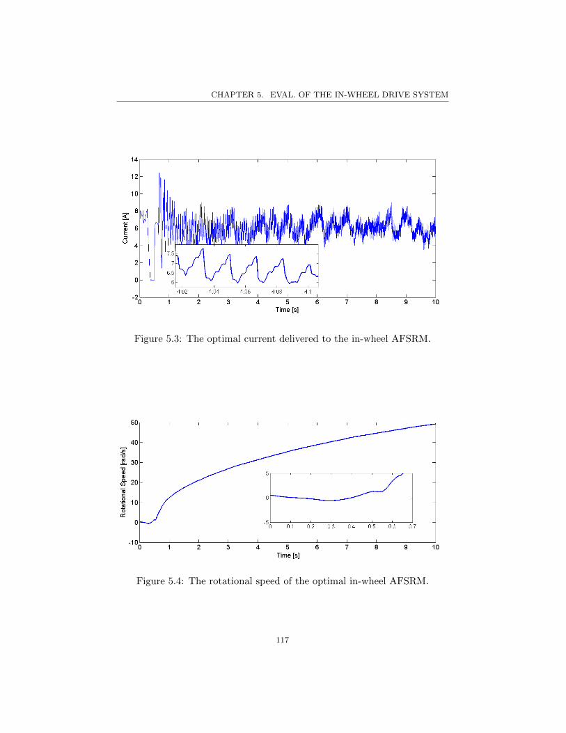
CHAPTER 5. EVAL. OF THE IN-WHEEL DRIVE SYSTEM
Figure 5.3: The optimal current delivered to the in-wheel AFSRM.
Figure 5.4: The rotational speed of the optimal in-wheel AFSRM.
117

CHAPTER 5. EVAL. OF THE IN-WHEEL DRIVE SYSTEM
Figure 5.5: The vertical force produced by a single phase of the optimalin-wheel AFSRM.
Figure 5.6: The vertical force produced by the optimal in-wheel AFSRM.
118

CHAPTER 5. EVAL. OF THE IN-WHEEL DRIVE SYSTEM
Figure 5.7: Power spectrum of the vehicle suspension with switch-on angleat −22.5 [deg], and switch-off angle at 22.5 [deg], for maximum torque.
Figure 5.8: Power spectrum of the vehicle suspension with switch-on angleat −12.5 [deg], and switch-off angle at 18.5 [deg], for minimum torque ripple.
119

CHAPTER 5. EVAL. OF THE IN-WHEEL DRIVE SYSTEM
Figure 5.9: The contact force of the vehicle tire with maximum torque, andwith minimum ripple.
Figure 5.10: The yaw rate of the full vehicle model with 2DOF, and 3DOFsuspension systems.
120

CHAPTER 5. EVAL. OF THE IN-WHEEL DRIVE SYSTEM
Figure 5.11: The path of vehicle models using both 2DOF, and 3DOF sus-pension systems.
Gradability
The gradability requirement is defined by
Gradability = 100 tan(sin−1(P/W )) (5.30)
where the total mass is equal to the curb mass plus two passengers weighinga total of 332 [lbs]. The weight is then W = 3497 [lbs], or 15556 [N ]. Thepropulsion force needed to overcome the weight of the vehicle on a 25% slopeis then
P = 15556 sin(tan−1(0.25)) = 3772.9 [N ]. (5.31)
In order to deliver that quantity of force at the outer edge of the tire(11.75 [in] radius, or 0.298 [m]), the motor must provide 1127 [N · m] oftorque. Distributing that amount between four wheels, we obtain a valueof 281.5 [N ·m] per wheel. The dynamic torque profile in Fig. 5.2 providesnearly 500 [N ·m] peak torque at full speed, which would be enough travelon a 47.8% grade.
121
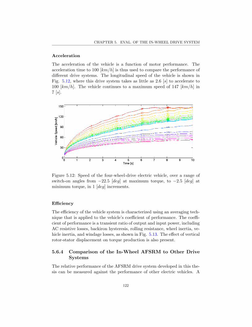
CHAPTER 5. EVAL. OF THE IN-WHEEL DRIVE SYSTEM
Acceleration
The acceleration of the vehicle is a function of motor performance. Theacceleration time to 100 [km/h] is thus used to compare the performance ofdifferent drive systems. The longitudinal speed of the vehicle is shown inFig. 5.12, where this drive system takes as little as 2.6 [s] to accelerate to100 [km/h]. The vehicle continues to a maximum speed of 147 [km/h] in7 [s].
Figure 5.12: Speed of the four-wheel-drive electric vehicle, over a range ofswitch-on angles from −22.5 [deg] at maximum torque, to −2.5 [deg] atminimum torque, in 1 [deg] increments.
Efficiency
The efficiency of the vehicle system is characterized using an averaging tech-nique that is applied to the vehicle’s coefficient of performance. The coeffi-cient of performance is a transient ratio of output and input power, includingAC resistive losses, backiron hysteresis, rolling resistance, wheel inertia, ve-hicle inertia, and windage losses, as shown in Fig. 5.13. The effect of verticalrotor-stator displacement on torque production is also present.
5.6.4 Comparison of the In-Wheel AFSRM to Other DriveSystems
The relative performance of the AFSRM drive system developed in this the-sis can be measured against the performance of other electric vehicles. A
122
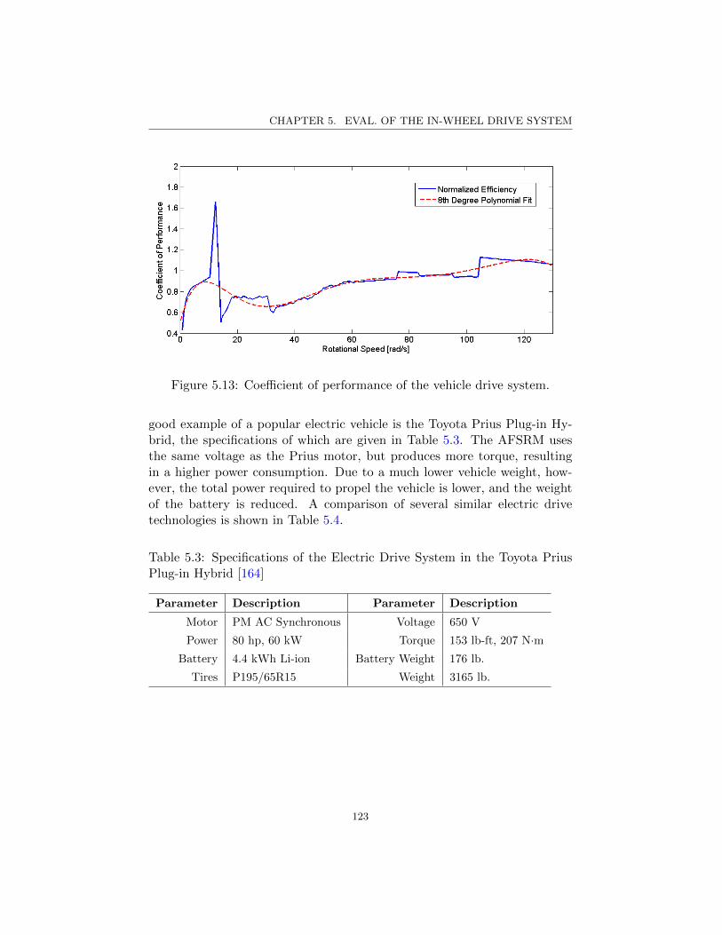
CHAPTER 5. EVAL. OF THE IN-WHEEL DRIVE SYSTEM
Figure 5.13: Coefficient of performance of the vehicle drive system.
good example of a popular electric vehicle is the Toyota Prius Plug-in Hy-brid, the specifications of which are given in Table 5.3. The AFSRM usesthe same voltage as the Prius motor, but produces more torque, resultingin a higher power consumption. Due to a much lower vehicle weight, how-ever, the total power required to propel the vehicle is lower, and the weightof the battery is reduced. A comparison of several similar electric drivetechnologies is shown in Table 5.4.
Table 5.3: Specifications of the Electric Drive System in the Toyota PriusPlug-in Hybrid [164]
Parameter Description Parameter Description
Motor PM AC Synchronous Voltage 650 V
Power 80 hp, 60 kW Torque 153 lb-ft, 207 N·mBattery 4.4 kWh Li-ion Battery Weight 176 lb.
Tires P195/65R15 Weight 3165 lb.
123

CHAPTER 5. EVAL. OF THE IN-WHEEL DRIVE SYSTEM
Table 5.4: Comparison of Electric Drive Systems
Parameter AFSRM Protean [28] AFPM [32] Prius [164]
Peak Torque, [N ·m] 2500 800 83.16 −Cont. Torque, [N ·m] ≈ 500 475 78.74 207
Voltage, [V ] 650 380 − 650
Efficiency > 95% − 82% −Weight, [kg] 40 31 10 −
124

Chapter 6
Conclusions and FutureWork
6.1 Conclusions
This thesis has developed a transient simulation model of a semi-anhystereticAFSRM using electromagnetic, mechanical, and thermal analysis. A sub-sequent evaluation of the in-wheel AFSRM drive system has proven thatit is useful for electric vehicle applications. A review of alternative motortopologies reinforces this claim, and provides evidence that the AFSRMis the best motor topology for in-wheel drive systems due to its low cost,material composition, durability, high efficiency, and simple construction.
The AFSRM geometry is selected based on a set of qualitative designconsiderations that are used to simplify the quantitative design process.These considerations are developed using fundamental physical motivationsdrawn from Maxwell’s stress tensor and a simple MEC model. Copper wasselected for the field windings and an SLSMC was selected for the backironbased on the geometry, application, and performance requirement of themachine.
The static AFSRM model is developed using a integral inductance func-tion and a comprehensive set of electric, magnetic, and mechanical lossmodels. The inductance function is developed by this thesis to fill a gap inthe analytic design process which has traditionally been occupied by FEA.The benefits and drawbacks of the inductance function are discussed in thecontext of several analytic and numerical alternatives to clarify its purpose.
The dynamic AFSRM model is developed using a linear MEC and a dis-cretized design geometry. Rotations and displacements are selected based ona predefined discrete resolution, and elliptic flux paths are used to calculatethe inductance and back-EMF of the motor. The dynamic model is usedto generate lookup tables for important motor parameters which are usedby the transient AFSRM model, and by the transient model of the in-wheeldrive system.
125

CHAPTER 6. CONCLUSIONS AND FUTURE WORK
The optimal AFSRM design is identified by integrating the set of lossmodels into the AFSRM model, and then translating the complete modelinto an iterative static optimization procedure. Some drawbacks of staticoptimization include the abstraction of the back-EMF, and the generalityof the performance index used to evaluate design variations at each step inthe optimization procedure. The optimal static design is produced, and isshown to develop a peak torque of approximately 3000 [N ·m] per phase.
The AFSRM controller is produced using a set of switching angles and aninstantaneous fuzzy current-shaping system. A static switch-on angle anda dynamic switch-off angle are selected based on a dynamic optimizationof the average torque. An optimal fuzzy controller is then applied to eachphase of the motor model in order to reduce variations in the torque causedby rotor-stator displacement. The accuracy of the controller is limited bythe accuracy of the dynamic AFSRM model due to its linear treatment ofmagnetic flux.
The performance of the AFSRM is evaluated by using the transientmodel to calculate the dynamic torque, current, and efficiency of the mo-tor. FEA is used to calculate a more accurate static torque profile for thetransient model, including the effect of saturation. The motor is simulatedconsidering only inertial loading, given that the full load will be developedwhen the motor is placed into the in-wheel drive system.
An integrated mechanical suspension is proposed as a component of thein-wheel AFSRM drive system. The parameters and performance of thesuspension system are identified and calculated. A semi-active control ap-proach is then suggested to improve ride comfort and handling for vehicleswith in-wheel drive systems. The road holding and ride comfort are eval-uated using a vehicle model composed of two coupled 3DOF quarter-carsuspension systems, including the semi-active controller. The suspensionsystem is shown to reduce automotive NVH.
The performance of the complete in-wheel AFSRM drive system is eval-uated using a transient vehicle model that includes handling, suspension,and propulsion dynamics. The effects of each subsystem on the other sub-systems are included to present the most comprehensive picture of the drivesystem. The handling model is used to show the improvement in steeringand road holding due to the semi-active suspension controller and the in-tegrated mechanical suspension system. The vehicle can accelerate from0 − 100 [km/h] in 2.6 [s], not considering wheel spin. The transient coeffi-cient of performance that characterizes the efficiency of the in-wheel drivesystem is > 95% in the ideal scenario.
126

CHAPTER 6. CONCLUSIONS AND FUTURE WORK
6.2 Recommendations for Future Work
There are three primary areas of improvement that could be completed infuture work. The first improvement is in regard to the optimization process.A dynamic optimization could be developed as a component of the transientSimulink model of the in-wheel drive system. This type of optimization isrestricted by its inherent computational overhead.
The second improvement involves the dynamic AFSRM model. A bettermodel that accounts for nonlinear magnetic saturation needs to be devel-oped. The back-EMF and inductance calculations from that model need tobe normalized to agree with the static torque curve produced using FEA.
The third improvement pertains to the phase current control system.The switch-on angle should be modified to include dynamic considerations,and the final control system needs to be re-optimized for the improved dy-namic AFSRM model. A more controllable motor is expected to result fromthis process.
127

Bibliography
[1] M. Ehsani, K. Rahman, and H. Toliyat, “Propulsion system designof electric and hybrid vehicles,” IEEE Transactions on IndustrialElectronics, vol. 44, no. 1, pp. 19–27, 1997. doi: 10.1109/41.557495(see p. 1).
[2] G. Offer, D. Howey, M. Contestabile, R. Clague, and N. Bran-don, “Comparative analysis of battery electric, hydrogen fuel celland hybrid vehicles in a future sustainable road transport sys-tem,” Energy Policy, vol. 38, no. 1, pp. 24–29, Jan. 2010. doi:10.1016/j.enpol.2009.08.040 (see p. 1).
[3] J. Jansson, “Consumer Eco-Innovation Adoption: Assessing Attitu-dinal Factors and Perceived Product Characteristics,” vol. 210, no.July 2010, pp. 192–210, 2011. doi: 10.1002/bse (see p. 1).
[4] P. Lemieux, R. Guthrie, and M. Isac, “Optimizing Soft MagneticComposites for Power Frequency Applications and Power-Trains,”Journal of the Minerals, Metals and Materials Society, vol. 64, no.3, pp. 374–387, Mar. 2012. doi: 10.1007/s11837-012-0262-z (seepp. 2, 11, 27).
[5] M. Takemoto, H. Suzuki, A. Chiba, T. Fukao, and M. Rahman, “Im-proved analysis of a bearingless switched reluctance motor,” IEEETransactions on Industry Applications, vol. 37, no. 1, pp. 26–34, 2001.doi: 10.1109/28.903123 (see pp. 2, 27, 38).
[6] A. Omekanda, “Robust torque and torque-per-inertia optimizationof a switched reluctance motor using the Taguchi methods,” IEEETransactions on Industry Applications, vol. 42, no. 2, pp. 473–478,Mar. 2006. doi: 10.1109/TIA.2006.870031 (see pp. 2, 27, 38, 39,52).
[7] P. Rasmussen, F Blaabjerg, J. Pedersen, and F Jensen, “Switchedreluctance-shark machines-more torque and less acoustic noise,” inConference Record of the 2000 IEEE Industry Applications Confer-ence. Thirty-Fifth IAS Annual Meeting and World Conference onIndustrial Applications of Electrical Energy (Cat. No.00CH37129),vol. 1, IEEE, 2000, pp. 93–98. doi: 10.1109/IAS.2000.881031 (seep. 2).
128

BIBLIOGRAPHY
[8] J Corda, A. Tataru, P. Rasmussen, and E Ritchie, “Analytical esti-mation of torque enhancement of the SR machine with saw-shaped(shark) pole surfaces,” IEE Proceedings - Electric Power Applica-tions, vol. 151, no. 2, p. 223, 2004. doi: 10.1049/ip-epa:20040018(see p. 2).
[9] J. Eastham, M. Balchin, T. Betzer, H. Lai, and S. Gair, “Disc motorwith reduced unsprung mass for direct EV wheel drive,” in Proceed-ings of the IEEE International Symposium on Industrial Electronics,vol. 2, IEEE, 1995, pp. 569–573. doi: 10.1109/ISIE.1995.497248(see p. 2).
[10] B Hredzak, S Gair, and J. Eastham, “Elimination of torque pulsationsin a direct drive EV wheel motor,” IEEE Transactions on Magnetics,vol. 32, no. 5, pp. 5010–5012, 1996. doi: 10.1109/20.539359 (seepp. 2, 11, 12, 59).
[11] B Hredzak, “Variable structure control of a disc motor with lateralrotor movement,” in 6th International Conference on Power Elec-tronics and Variable Speed Drives, vol. 1996, IEE, 1996, pp. 197–202.doi: 10.1049/cp:19960912 (see pp. 2, 59).
[12] D. van Schalkwyk and M. Kamper, “Effect of Hub Motor Masson Stability and Comfort of Electric Vehicles,” in 2006 IEEE Ve-hicle Power and Propulsion Conference, Department of Electricaland Electronic Engineering, University of Stellenbosch, Stellenbosch:IEEE, Sep. 2006, pp. 1–6. doi: 10.1109/VPPC.2006.364297 (seepp. 2, 10, 101).
[13] S. M. Savaresi and C. Spelta, “A Single-Sensor Control Strategy forSemi-Active Suspensions,” IEEE Transactions on Control SystemsTechnology, vol. 17, no. 1, pp. 143–152, Jan. 2009. doi: 10.1109/TCST.2008.906313 (see pp. 2, 82, 95, 96).
[14] Y. Luo and D. Tan, “Study on the Dynamics of the In-Wheel MotorSystem,” IEEE Transactions on Vehicular Technology, vol. 61, no.8, pp. 3510–3518, Oct. 2012. doi: 10.1109/TVT.2012.2207414 (seepp. 2, 12, 82).
[15] M. Abbasian, M. Moallem, and B. Fahimi, “Double-Stator SwitchedReluctance Machines (DSSRM): Fundamentals and Magnetic ForceAnalysis,” IEEE Transactions on Energy Conversion, vol. 25, no. 3,pp. 589–597, 2010 (see pp. 3, 15, 16, 18, 27).
[16] W. Adams, Electric Motor, 1884 (see p. 4).
129

BIBLIOGRAPHY
[17] F. Porsche, Improvements in or relating to Electrically Driven RoadVehicles, 1900 (see p. 4).
[18] Porsche, Prof. Ferdinand Porsche Created the First Functional Hy-brid Car, 2011 (see p. 5).
[19] Protean Electric, Protean Drive PD18 Performance Character, 2012(see p. 5).
[20] —, Technical Art: Front view of the Protean Drive in-wheel motorwith a cutaway displaying the integrated micro inverters, 2013 (seep. 6).
[21] Michelin, Michelin Active Wheel, 2008 (see p. 7).
[22] Fraunhofer IFAM, Radnabenmotor am Fraunhofer Demonstrator-fahrzeug Frecc0, 2013 (see p. 7).
[23] Siemens, Siemens VDO Engine, 2007 (see p. 8).
[24] H. Shimizu, Succeeded to achieve 333km of range per charge with theAdvanced Development Model, 2011 (see p. 8).
[25] R. Vandana and B. G. Fernandes, “Optimal sizing of motor Batterysystem for in wheel electric vehicles,” in IECON 2010 - 36th AnnualConference on IEEE Industrial Electronics Society, IEEE, Nov. 2010,pp. 2510–2515. doi: 10.1109/IECON.2010.5675157 (see pp. 9, 11).
[26] K. Cakir and A. Sabanovic, “In-wheel motor design for electric ve-hicles,” in 9th IEEE International Workshop on Advanced MotionControl, 2006., IEEE, 2006, pp. 613–618. doi: 10.1109/AMC.2006.1631730 (see pp. 9, 11, 15, 67).
[27] K. Rahman, N. Patel, T. Ward, J. Nagashima, F. Caricchi, andF. Crescimbini, “Application of Direct-Drive Wheel Motor for FuelCell Electric and Hybrid Electric Vehicle Propulsion System,” IEEETransactions on Industry Applications, vol. 42, no. 5, pp. 1185–1192,Sep. 2006. doi: 10.1109/TIA.2006.880886 (see pp. 9, 11, 15).
[28] C. Ifedi, B. Mecrow, S. Brockway, G. Boast, G. Atkinson, and D.Kostic-Perovic, “Fault tolerant in-wheel motor topologies for highperformance electric vehicles,” in 2011 IEEE International Elec-tric Machines & Drives Conference (IEMDC), IEEE, May 2011,pp. 1310–1315. doi: 10.1109/IEMDC.2011.5994794 (see pp. 9–11, 101, 121).
130

BIBLIOGRAPHY
[29] A. J. Rix and M. J. Kamper, “Radial-Flux Permanent-Magnet HubDrives: A Comparison Based on Stator and Rotor Topologies,” IEEETransactions on Industrial Electronics, vol. 59, no. 6, pp. 2475–2483,Jun. 2012. doi: 10.1109/TIE.2011.2161654 (see pp. 9–11).
[30] S. Rinderknecht and T. Meier, “Electric power train configurationsand their transmission systems,” Speedam 2010, pp. 1564–1568, Jun.2010. doi: 10.1109/SPEEDAM.2010.5542276 (see p. 9).
[31] A. Haddoun, M. Benbouzid, D. Diallo, R. Abdessemed, J. Ghouili,and K. Srairi, “Design and implementation of an Electric Differentialfor traction application,” in 2010 IEEE Vehicle Power and PropulsionConference, IEEE, Sep. 2010, pp. 1–6. doi: 10.1109/VPPC.2010.5729056 (see pp. 9, 27).
[32] Y.-P. Yang, Y.-P. Luh, and C.-H. Cheung, “Design and Control ofAxial-Flux Brushless DC Wheel Motors for Electric VehiclesPart I:Multiobjective Optimal Design and Analysis,” IEEE Transactionson Magnetics, vol. 40, no. 4, pp. 1873–1882, Jul. 2004. doi: 10.1109/TMAG.2004.828164 (see pp. 9–11, 27, 52, 67, 121).
[33] X. D. Xue, K. W. E. Cheng, T. W. Ng, and N. C. Cheung,“Multi-Objective Optimization Design of In-Wheel Switched Re-luctance Motors in Electric Vehicles,” IEEE Transactions on In-dustrial Electronics, vol. 57, no. 9, pp. 2980–2987, Sep. 2010. doi:10.1109/TIE.2010.2051390 (see pp. 9, 11, 52).
[34] C. Ciurtin, D. Ilea, F. Gillon, P. Brochet, and M. M. Radulescu,“Comparative Design of Radial-Flux and Axial-Flux Switched Re-luctance Motors,” in 2nd International Conference on Modern PowerSystems, Cluj-Napoca, Romania, 2008, pp. 12–14 (see p. 9).
[35] F. Profumo and A. Tenconi, “Axial flux machines drives: a new viablesolution for electric cars,” IEEE Transactions on Industrial Electron-ics, vol. 44, no. 1, pp. 39–45, 1997. doi: 10.1109/41.557497 (seep. 9).
[36] Y. Ozoglu, M. Garip, and E. Mese, “New pole tip shapes mitigatingtorque ripple in short pitched and fully pitched switched reluctancemotors,” in Conference Record of the 2002 IEEE Industry Applica-tions Conference. 37th IAS Annual Meeting (Cat. No.02CH37344),vol. 1, IEEE, 2002, pp. 43–50. doi: 10.1109/IAS.2002.1044065 (seepp. 9, 16, 52).
131

BIBLIOGRAPHY
[37] D Andessner and W Amrhein, “Current feed optimization for theswitched permanent magnet reluctance machine,” in 2008 18th Inter-national Conference on Electrical Machines, IEEE, Sep. 2008, pp. 1–6. doi: 10.1109/ICELMACH.2008.4799908 (see pp. 9, 10).
[38] T. Miller, “Optimal design of switched reluctance motors,” IEEETransactions on Industrial Electronics, vol. 49, no. 1, pp. 15–27, 2002.doi: 10.1109/41.982244 (see pp. 9, 10, 27, 37, 52, 67).
[39] M. Zeraoulia, M. E. H. Benbouzid, and D. Diallo, “Electric MotorDrive Selection Issues for HEV Propulsion Systems: A ComparativeStudy,” IEEE Transactions on Vehicular Technology, vol. 55, no. 6,pp. 1756–1764, Nov. 2006. doi: 10.1109/TVT.2006.878719 (seep. 9).
[40] K. Rahman, B. Fahimi, G. Suresh, a.V. Rajarathnam, and M. Ehsani,“Advantages of switched reluctance motor applications to EV andHEV: design and control issues,” Conference Record of 1998 IEEEIndustry Applications Conference. Thirty-Third IAS Annual Meeting(Cat. No.98CH36242), vol. 1, pp. 327–334, 1998. doi: 10.1109/IAS.1998.732314 (see p. 9).
[41] K. Kiyota, H. Sugimoto, and A. Chiba, “Comparison of energy con-sumption of SRM and IPMSM in automotive driving schedules,” in2012 IEEE Energy Conversion Congress and Exposition (ECCE),IEEE, Sep. 2012, pp. 853–860. doi: 10.1109/ECCE.2012.6342729(see pp. 9, 10, 67).
[42] V. Petrus, A. C. Pop, C. S. Martis, J. Gyselinck, and V. Iancu,“Design and comparison of different Switched Reluctance Machinetopologies for electric vehicle propulsion,” in The XIX InternationalConference on Electrical Machines - ICEM 2010, IEEE, Sep. 2010,pp. 1–6. doi: 10.1109/ICELMACH.2010.5608008 (see pp. 9, 11, 16,52, 67).
[43] Y.-P. Yang, J.-P. Wang, S.-W. Wu, and Y.-P. Luh, “Design andControl of Axial-Flux Brushless DC Wheel Motors for Electric Ve-hiclesPart II: Optimal Current Waveforms and Performance Test,”IEEE Transactions on Magnetics, vol. 40, no. 4, pp. 1883–1891, Jul.2004. doi: 10.1109/TMAG.2004.828165 (see pp. 9, 52).
[44] T. Miura, S. Chino, M. Takemoto, and S. Ogasawara, “A ferrite per-manent magnet axial gap motor with segmented rotor structure forthe next generation hybrid vehicle,” The XIX International Confer-
132

BIBLIOGRAPHY
ence on Electrical Machines - ICEM 2010, pp. 1–6, Sep. 2010. doi:10.1109/ICELMACH.2010.5607864 (see pp. 9, 10).
[45] B. Virlan, A. Simion, L. Livadaru, S. Benelghali, and R. Out-bib, “Analysis of a three phase induction motor with outer ro-tor for multi-speed applications,” 2012 XXth International Con-ference on Electrical Machines, pp. 411–417, Sep. 2012. doi:10.1109/ICElMach.2012.6349900 (see pp. 9, 10).
[46] M. Popescu, D. G. Dorrell, and P. Holik, “Improving the startingtorque in external-rotor induction motors using an outer can,” inThe 3rd IET International Conference on Power Electronics, vol. 2,2006, pp. 531–535 (see p. 10).
[47] I. Tarimer and C. Ocak, “Performance Comparision of Internal andExternal Rotor Structured Wind Generators Mounted from SamePermanent Magnets on Same Geometry,” Electronics and ElectricalEngineering, vol. 4, no. 92, pp. 65–70, 2009 (see p. 10).
[48] L. Zhu, S. Jiang, Z. Zhu, and C. Chan, “Analytical Methods forMinimizing Cogging Torque in Permanent-Magnet Machines,” IEEETransactions on Magnetics, vol. 45, no. 4, pp. 2023–2031, Apr. 2009.doi: 10.1109/TMAG.2008.2011363 (see p. 10).
[49] Z. Zhu and D. Howe, “Halbach permanent magnet machines and ap-plications: a review,” IEE Proceedings - Electric Power Applications,vol. 148, no. 4, p. 299, 2001. doi: 10.1049/ip-epa:20010479 (seep. 10).
[50] S.-M. Hwang, J.-B. Eom, G.-B. Hwang, W.-B. Jeong, and Y.-H. Jung,“Cogging torque and acoustic noise reduction in permanent magnetmotors by teeth pairing,” IEEE Transactions on Magnetics, vol. 36,no. 5, pp. 3144–3146, 2000. doi: 10.1109/20.908714 (see p. 10).
[51] R. N. Tuncay, O. Ustun, M. Yilmaz, C. Gokce, and U. Karakaya,“Design and implementation of an electric drive system for in-wheelmotor electric vehicle applications,” in 2011 IEEE Vehicle Powerand Propulsion Conference, IEEE, Sep. 2011, pp. 1–6. doi: 10.1109/VPPC.2011.6043070 (see pp. 10, 11).
[52] H. C. Lovatt, D. Elton, L. Cahill, A. Stumpf, A. Kulkarni, A. Kapoor,M. Ektesabi, H. Mazumder, T. Dittmar, and G. White, “Design pro-cedure for low cost, low mass, direct drive, in-wheel motor drivetrainsfor electric and hybrid vehicles,” in IECON 2011 - 37th Annual Con-
133
BIBLIOGRAPHY
ference of the IEEE Industrial Electronics Society, IEEE, Nov. 2011,pp. 4558–4562. doi: 10.1109/IECON.2011.6120061 (see pp. 10, 11).
[53] R. Wrobel, J. Goss, A. Mlot, and P. Mellor, “Design considerationsof a brushless open-slot radial-flux PM hub motor,” in 2012 IEEEEnergy Conversion Congress and Exposition (ECCE), IEEE, Sep.2012, pp. 3678–3685. doi: 10.1109/ECCE.2012.6342479 (see pp. 10,11).
[54] R. Wrobel, P. H. Mellor, N. McNeill, and D. a. Staton, “ThermalPerformance of an Open-Slot Modular-Wound Machine With Exter-nal Rotor,” IEEE Transactions on Energy Conversion, vol. 25, no.2, pp. 403–411, Jun. 2010. doi: 10.1109/TEC.2010.2047041 (seepp. 11, 67).
[55] R. Madhavan and B. G. Fernandes, “A novel axial flux segmentedSRM for electric vehicle application,” in The XIX International Con-ference on Electrical Machines - ICEM 2010, IEEE, Sep. 2010, pp. 1–6. doi: 10.1109/ICELMACH.2010.5608140 (see p. 11).
[56] S. A. Zulkifli, N. Saad, S. Mohd, and A. R. A. Aziz, “Split-parallel in-wheel-motor retrofit hybrid electric vehicle,” in 2012 IEEE Interna-tional Power Engineering and Optimization Conference, IEEE, Jun.2012, pp. 11–16. doi: 10.1109/PEOCO.2012.6230915 (see p. 11).
[57] D Larbalestier, A Gurevich, D. M. Feldmann, and A Polyan-skii, “High-Tc superconducting materials for electric power appli-cations.,” Nature, vol. 414, no. 6861, pp. 368–77, Nov. 2001. doi:10.1038/35104654 (see p. 11).
[58] A. P. Malozemoff, S Fleshler, M Rupich, C Thieme, X Li, W Zhang,A Otto, J Maguire, D Folts, J Yuan, H.-P. Kraemer, W Schmidt,M Wohlfart, and H.-W. Neumueller, “Progress in high temperaturesuperconductor coated conductors and their applications,” Supercon-ductor Science and Technology, vol. 21, no. 3, pp. 1–7, Mar. 2008. doi:10.1088/0953-2048/21/3/034005 (see p. 11).
[59] M. Anderson and D. Harty, “Unsprung Mass with In-Wheel Motors- Myths and Realities,” in AVEC 10, 2010, pp. 261–266 (see pp. 12,101).
[60] M. Takemoto, A. Chiba, H. Akagi, and T. Fukao, “Radial Force andTorque of a Bearingless Switched Reluctance Motor Operating ina Region of Magnetic Saturation,” IEEE Transactions on Industry
134

BIBLIOGRAPHY
Applications, vol. 40, no. 1, pp. 103–112, Jan. 2004. doi: 10.110
9/TIA.2003.821816 (see p. 15).
[61] K. Bienkowski, B. Bucki, A. Rogalski, and A. Pochanke, “Five phaseswitched reluctance motor with short flux path for low speed appli-cations and mechatronics,” Warsaw (see p. 15).
[62] X. Deng, Q. Yuan, J. Lu, and X. Li, “Study on the Reduction ofVibration and Acoustic Noise in the Switched Reluctance Motor,” in2009 Asia-Pacific Power and Energy Engineering Conference, IEEE,Mar. 2009, pp. 1–4. doi: 10.1109/APPEEC.2009.4918849 (see pp. 15,16, 27).
[63] M.-T. Khor, R. Sotudeh, and D. Lee, “Switched Reluctance MotorBased on Short Flux Path Control Method,” in Universities PowerEngineering Conference, University of Hertfordshire, Hertfordshire,United Kingdom, 2004, pp. 559–562 (see pp. 15, 16, 52).
[64] S.-H. Mao and M.-C. Tsai, “A novel switched reluctance motor withC-core stators,” IEEE Transactions on Magnetics, vol. 41, no. 12,pp. 4413–4420, Dec. 2005. doi: 10.1109/TMAG.2005.858372 (seepp. 15, 16, 52).
[65] E. Swint and R. Krishnan, “Two-Phase SR Drive with Flux-ReversalFree Stator and Balanced Normal Forces,” in 2008 IEEE IndustryApplications Society Annual Meeting, IEEE, Oct. 2008, pp. 1–6. doi:10.1109/08IAS.2008.70 (see pp. 15, 16).
[66] W. Jiang, M. Moallem, B. Fahimi, and S. Pekarek, “QualitativeInvestigation of Force Density Components in ElectromechanicalEnergy Conversion Process,” IECON 2006 - 32nd Annual Confer-ence on IEEE Industrial Electronics, pp. 1113–1118, Nov. 2006. doi:10.1109/IECON.2006.347809 (see p. 16).
[67] X. Cao, Z. Deng, G. Yang, and X. Wang, “Independent Con-trol of Average Torque and Radial Force in Bearingless Switched-Reluctance Motors With Hybrid Excitations,” IEEE Transactionson Power Electronics, vol. 24, no. 5, pp. 1376–1385, May 2009. doi:10.1109/TPEL.2009.2016568 (see pp. 16, 27, 67).
[68] P. Rafajdus and I. Zrak, “Analysis Of The Switched Reluctance Mo-tor (SRM) Parameters,” Journal of Electrical Engineering, vol. 55,no. 7, pp. 195–200, 2004 (see p. 16).
135

BIBLIOGRAPHY
[69] R. Krishnan and R. Bedingfield, “Dynamic analysis of an SRMdrive system,” in Conference Record of the 1991 IEEE Industry Ap-plications Society Annual Meeting, IEEE, 1991, pp. 265–271. doi:10.1109/IAS.1991.178165 (see pp. 16, 27, 37, 39).
[70] A. R. C. S. Babu and K. R. Rajagopal, “Slanted and saw-toothed sta-tor poles for improved performance of doubly salient permanent mag-net motor,” Journal of Applied Physics, vol. 97, no. 10, 10Q514(1–3),2005. doi: 10.1063/1.1860831 (see p. 16).
[71] Y. Wang, J. Shen, W. Fei, and Z. Fang, “Reduction of Cogging Torquein Permanent Magnet Flux-Switching Machines,” Journal of Electro-magnetic Analysis & Applications, no. 1, pp. 11–14, 2009 (see p. 16).
[72] B. Bilgin, A. Emadi, and M. Krishnamurthy, “Design Considerationsfor Switched Reluctance Machines With a Higher Number of RotorPoles,” IEEE Transactions on Industrial Electronics, vol. 59, no. 10,pp. 3745–3756, Oct. 2012. doi: 10.1109/TIE.2011.2141102 (seep. 16).
[73] D. Hanselman, “Effect of skew, pole count and slot count on brushlessmotor radial force, cogging torque and back EMF,” IEE Proceedings- Electric Power Applications, vol. 144, no. 5, p. 325, 1997. doi: 10.1049/ip-epa:19971205 (see pp. 16, 52).
[74] M. B Belhadi, A Kolli, G. Krebs, and C. Marchand, “Evaluation oftorque-speed curve of switched reluctance motor with segmental ro-tor,” in 2012 XXth International Conference on Electrical Machines,IEEE, Sep. 2012, pp. 250–255. doi: 10.1109/ICElMach.2012.6349873 (see pp. 16, 67).
[75] P. Desai, M. Krishnamurthy, N. Schofield, and A. Emadi, “NovelSwitched Reluctance Machine Configuration With Higher Number ofRotor Poles Than Stator Poles: Concept to Implementation,” IEEETransactions on Industrial Electronics, vol. 57, no. 2, pp. 649–659,Feb. 2010. doi: 10.1109/TIE.2009.2034678 (see p. 16).
[76] J. Lee, H. Kim, B. Kwon, and B. Kim, “New Rotor Shape Design forMinimum Torque Ripple of SRM Using FEM,” IEEE Transactionson Magnetics, vol. 40, no. 2, pp. 754–757, Mar. 2004. doi: 10.1109/TMAG.2004.824803 (see pp. 16, 27, 52).
136

BIBLIOGRAPHY
[77] A Deihimi, S Farhangi, and G Henneberger, “A general non-linear model of switched reluctance motor with mutual cou-pling and multiphase excitation,” Electrical Engineering (Archivfur Elektrotechnik), vol. 84, no. 3, pp. 143–158, Jul. 2002. doi:10.1007/s00202-001-0113-3 (see pp. 16, 27, 39, 67).
[78] J Cros and P Viarouge, “New Structures of Polyphase Claw-PoleMachines,” IEEE Transactions on Industry Applications, vol. 40, no.1, pp. 113–120, Jan. 2004. doi: 10.1109/TIA.2003.821648 (seepp. 16, 52).
[79] A. Radun, “Design considerations for the switched reluctance motor,”IEEE Transactions on Industry Applications, vol. 31, no. 5, pp. 1079–1087, 1995. doi: 10.1109/28.464522 (see pp. 16, 27).
[80] M. Moallem and G. Dawson, “An improved magnetic equivalent cir-cuit method for predicting the characteristics of highly saturated elec-tromagnetic devices,” IEEE Transactions on Magnetics, vol. 34, no.5, pp. 3632–3635, 1998. doi: 10.1109/20.717858 (see p. 16).
[81] C. Morrison, M. Siebert, and E. Ho, “Electromagnetic Forces in aHybrid Magnetic-Bearing Switched-Reluctance Motor,” IEEE Trans-actions on Magnetics, vol. 44, no. 12, pp. 4626–4638, Dec. 2008. doi:10.1109/TMAG.2008.2002891 (see p. 27).
[82] N. Fuengwarodsakul, B. Gu, S. Schroeder, R. De Do, and K Nam,“Simplified Unbalanced Force Calculation in Switched ReluctanceMachines Using Electromagnetic Circuit Model,” in IEEE Interna-tional Conference on Electric Machines and Drives, 2005., IEEE,2005, pp. 498–503. doi: 10.1109/IEMDC.2005.195769 (see p. 27).
[83] J. Ferreira, “Improved analytical modeling of conductive losses inmagnetic components,” IEEE Transactions on Power Electronics,vol. 9, no. 1, pp. 127–131, 1994. doi: 10 . 1109 / 63 . 285503 (seepp. 29, 30).
[84] A. Urling, V. Niemela, G. Skutt, and T. Wilson, “Characterizinghigh-frequency effects in transformer windings-a guide to several sig-nificant articles,” in Proceedings, Fourth Annual IEEE Applied PowerElectronics Conference and Exposition, IEEE, 1989, pp. 373–385. doi:10.1109/APEC.1989.36989 (see p. 30).
137

BIBLIOGRAPHY
[85] C. Sullivan, “An improved calculation of proximity-effect loss in high-frequency windings of round conductors,” in IEEE 34th Annual Con-ference on Power Electronics Specialist, 2003. PESC ’03., vol. 2,IEEE, 2003, pp. 853–860. doi: 10.1109/PESC.2003.1218168 (seepp. 30, 31).
[86] P. Dowell, “Effects of eddy currents in transformer windings,” Pro-ceedings of the Institution of Electrical Engineers, vol. 113, no. 8,p. 1387, 1966. doi: 10.1049/piee.1966.0236 (see p. 30).
[87] R. L. Stoll, D Ph, and C Eng, “Approximate formula for the eddy-current loss induced in a long conductor of rectangular cross- sectionby a transverse magnetic field,” vol. 116, no. 6, pp. 1003–1008, 1969(see p. 30).
[88] J. V. Leite, N Sadowski, N. J. Batistela, J. P. A. Bastos, A. A. D.Espındola, and A. O. J. A. Model, “Inverse Jiles Atherton VectorHysteresis Model,” vol. 40, no. 4, pp. 1769–1775, 2004 (see p. 33).
[89] J. Izydorczyk, “Simulation of soft magnetic materials by SPICE,”MELECON 2006 - 2006 IEEE Mediterranean Electrotechnical Con-ference, pp. 141–144, 2006. doi: 10.1109/MELCON.2006.1653056(see p. 33).
[90] N. Sadowski, N. Batistela, J. Bastos, and M. Lajoie-Mazenc, “Aninverse Jiles-Atherton model to take into account hysteresis in time-stepping finite-element calculations,” IEEE Transactions on Magnet-ics, vol. 38, no. 2, pp. 797–800, Mar. 2002. doi: 10.1109/20.996206(see p. 33).
[91] S. E. Zirka, Y. I. Moroz, R. G. Harrison, and K. Chwastek, “Onphysical aspects of the Jiles-Atherton hysteresis models,” Journal ofApplied Physics, vol. 112, no. 4, p. 043 916, 2012. doi: 10.1063/1.4747915 (see p. 33).
[92] J. E. Vrancik, “Prediction of Windage Power Loss in Alternators,”NASA, Washington, D.C., Tech. Rep. October, 1968 (see p. 35).
[93] T. Cousseau, B. Graca, A. Campos, and J. Seabra, “Friction torquein grease lubricated thrust ball bearings,” Tribology International,vol. 44, no. 5, pp. 523–531, May 2011. doi: 10.1016/j.triboint.2010.06.013 (see pp. 36, 87).
[94] G. Kron, “Equivalent Circuits for the Hunting of Electrical Machin-ery,” Electrical Engineering, vol. 61, no. 5, pp. 290–296, 1942. doi:10.1109/EE.1942.6436294 (see p. 38).
138

BIBLIOGRAPHY
[95] R. Hoft, “Liapunov Stability Analysis of Reluctance Motors,” IEEETransactions on Power Apparatus and Systems, vol. PAS-87, no. 6,pp. 1485–1491, Jun. 1968. doi: 10.1109/TPAS.1968.292118 (seep. 38).
[96] B. Smith, “Some characteristics of a class of parametric reluctancemachines,” Proceedings of the Institution of Electrical Engineers, vol.126, no. 2, p. 162, 1979. doi: 10.1049/piee.1979.0036 (see p. 38).
[97] W. F. Ray and R. M. Davis, “Its fundamental behaviour , linearanalysis and cost implications,” 1973 (see p. 38).
[98] P. J. Lawrenson, D Sc, I. E. E. E. Fel, C Eng, and J. M. Stephenson,“Variable-speed switched reluctance motors,” vol. 127, no. 4, pp. 253–265, 1980 (see p. 38).
[99] F. Marignetti, “Coupled Electro Magnetic Thermal and Fluid Dy-namical Simulation of Axial Flux PM Synchronous Machines,” inCOMSOL Users Conference 2007, Grenoble, 2007 (see pp. 38, 67,68).
[100] Y. Zhang, J. Ruan, T. Huang, X. Yang, H. Zhu, and G. Yang, “Calcu-lation of Temperature Rise in Air-cooled Induction Motors Through3-D Coupled Electromagnetic Fluid-Dynamical and Thermal Finite-Element Analysis,” IEEE Transactions on Magnetics, vol. 48, no. 2,pp. 1047–1050, Feb. 2012. doi: 10.1109/TMAG.2011.2174433 (seepp. 38, 68).
[101] T. Lubin, S. Mezani, and A. Rezzoug, “Exact Analytical Methodfor Magnetic Field Computation in the Air Gap of CylindricalElectrical Machines Considering Slotting Effects,” IEEE Transac-tions on Magnetics, vol. 46, no. 4, pp. 1092–1099, Apr. 2010. doi:10.1109/TMAG.2009.2036257 (see p. 39).
[102] T. Lubin, S. Mezani, and A. Rezzoug, “Simple Analytical Expres-sions for the Force and Torque of Axial Magnetic Couplings,” IEEETransactions on Energy Conversion, vol. 27, no. 2, pp. 536–546, Jun.2012. doi: 10.1109/TEC.2012.2183372 (see p. 39).
[103] J. Johnson, a.V. Rajarathnam, H. Toliyat, S. Gopalakrishnan, andB. Fahimi, “Torque optimization for a SRM using winding functiontheory with a gap-dividing surface,” IAS ’96. Conference Record ofthe 1996 IEEE Industry Applications Conference Thirty-First IASAnnual Meeting, vol. 2, pp. 753–760, 1996. doi: 10.1109/IAS.1996.560170 (see pp. 39, 40).
139

BIBLIOGRAPHY
[104] T. Lubin, S. Mezani, and A. Rezzoug, “2D Analytical Calculation ofMagnetic Field and Electromagnetic,” pp. 1–12, 2012. doi: 10.1109/TMAG.2011.218091 (see p. 40).
[105] M. B. Villarino, “Ramanujan’s Perimeter of an Ellipse,” vol. 3, p. 12,Jun. 2005. arXiv:0506384 [math] (see p. 41).
[106] J. F. Gieras, R.-J. Wang, and M. J. Kamper, “Axial Flux PermanentMagnet Brushless Machines,” 2008. doi: 10.1007/978-1-4020-8227-6 (see p. 50).
[107] M. Inoue, Y. Kuroda, S. Nishimura, and H. Akita, “An evaluationof concentrated and distributed windings in interior PM and clawpole motors,” in 8th International Conference on Power Electronics- ECCE Asia, Jeju, Korea: IEEE, May 2011, pp. 176–183. doi: 10.1109/ICPE.2011.5944572 (see p. 52).
[108] B. Loop and S. Sudhoff, “Switched reluctance machine model usinginverse inductance characterization,” IEEE Transactions on IndustryApplications, vol. 39, no. 3, pp. 743–751, May 2003. doi: 10.110
9/TIA.2003.811785 (see p. 52).
[109] N. Schofield, S. A. Long, D. Howe, and M. McClelland, “Design of aSwitched Reluctance Machine for Extended Speed Operation,” IEEETransactions on Industry Applications, vol. 45, no. 1, pp. 116–122,2009. doi: 10.1109/TIA.2008.2009506 (see p. 59).
[110] H. Hannoun, M. Hilairet, and C. Marchand, “Design of an SRMSpeed Control Strategy for a Wide Range of Operating Speeds,”IEEE Transactions on Industrial Electronics, vol. 57, no. 9, pp. 2911–2921, Sep. 2010. doi: 10.1109/TIE.2009.2038396 (see p. 59).
[111] H. K. M. Khoi, J.-W. Ahn, and D.-H. Lee, “Current Control Schemeof High Speed SRM Using Low Resolution Encoder,” Journal ofPower Electronics, vol. 11, no. 4, pp. 520–526, Jul. 2011. doi:10.6113/JPE.2011.11.4.520 (see p. 59).
[112] T.-S. Chuang and C. Pollock, “Robust speed control of a switchedreluctance vector drive using variable structure approach,” IEEETransactions on Industrial Electronics, vol. 44, no. 6, pp. 800–808,1997. doi: 10.1109/41.649941 (see p. 59).
[113] B. Hredzak, S Gair, and J. Eastham, “Control of an EV drive withreduced unsprung mass,” IEE Proceedings - Electric Power Applica-tions, vol. 145, no. 6, p. 600, 1998. doi: 10.1049/ip-epa:19982012(see p. 60).
140

BIBLIOGRAPHY
[114] H. Le-Huy and P. Brunelle, “A versatile nonlinear switched reluc-tance motor model in Simulink using realistic and analytical mag-netization characteristics,” 31st Annual Conference of IEEE Indus-trial Electronics Society, 2005. IECON 2005., no. c, 6 pp. 2005. doi:10.1109/IECON.2005.1569136 (see p. 67).
[115] O. Ichinokura, S. Suyama, T. Watanabe, and H. Guo, “A new calcu-lation model of switched reluctance motor for use on SPICE,” IEEETransactions on Magnetics, vol. 37, no. 4, pp. 2834–2836, Jul. 2001.doi: 10.1109/20.951321 (see p. 67).
[116] I.-C. Vese, F. Marignetti, and M. Radulescu, “Multiphysics Approachto Numerical Modeling of a Permanent-Magnet Tubular Linear Mo-tor,” IEEE Transactions on Industrial Electronics, vol. 57, no. 1,pp. 320–326, Jan. 2010. doi: 10.1109/TIE.2009.2030206 (see p. 67).
[117] M. Fenot, Y. Bertin, E. Dorignac, and G. Lalizel, “A review of heattransfer between concentric rotating cylinders with or without ax-ial flow,” International Journal of Thermal Sciences, vol. 50, no. 7,pp. 1138–1155, Jul. 2011. doi: 10.1016/j.ijthermalsci.2011.02.013 (see p. 67).
[118] K. Hruska, V. Kindl, and R. Pechanek, “Concept, design and cou-pled electro-thermal analysis of new hybrid drive vehicle for publictransport,” in Proceedings of 14th International Power Electronicsand Motion Control Conference EPE-PEMC 2010, IEEE, Sep. 2010,pp. 5–8. doi: 10.1109/EPEPEMC.2010.5606895 (see pp. 67, 68).
[119] E. V. Kazmin, E. A. Lomonova, and J. J. H. Paulides, “BrushlessTraction PM Machines Using Commercial Drive Technology , Part I :Design Methodology and Motor Design,” in International Conferenceon Electrical Machines and Systems, Wuhan, 2008, pp. 3801–3809(see pp. 67, 68).
[120] R. Camilleri, D. Howey, and M. McCulloch, “Thermal limitations inair-cooled axial flux in-wheel motors for urban mobility vehicles: Apreliminary analysis,” 2012 Electrical Systems for Aircraft, Railwayand Ship Propulsion, pp. 1–8, Oct. 2012. doi: 10.1109/ESARS.2012.6387494 (see p. 68).
[121] F. Giulii Capponi, G. De Donato, and F. Caricchi, “Recent Advancesin Axial-Flux Permanent-Magnet Machine Technology,” IEEE Trans-actions on Industry Applications, vol. 48, no. 6, pp. 2190–2205, Nov.2012. doi: 10.1109/TIA.2012.2226854 (see p. 68).
141

BIBLIOGRAPHY
[122] L. Ye, D. Li, Y. Ma, and B. Jiao, “Design and Performance ofa Water-cooled Permanent Magnet Retarder for Heavy Vehicles,”IEEE Transactions on Energy Conversion, vol. 26, no. 3, pp. 953–958, Sep. 2011. doi: 10.1109/TEC.2011.2157347 (see p. 68).
[123] D. Joo, J.-H. Cho, K. Woo, B.-T. Kim, and D.-K. Kim, “Electro-magnetic Field and Thermal Linked Analysis of Interior Permanent-Magnet Synchronous Motor for Agricultural Electric Vehicle,” IEEETransactions on Magnetics, vol. 47, no. 10, pp. 4242–4245, Oct. 2011.doi: 10.1109/TMAG.2011.2149504 (see p. 68).
[124] P. Lemieux, O. Jude Delma, M. R. Dubois, and R. Guthrie, “Softmagnetic composite with Lamellar particles - Application to theClawpole Transverse-Flux Machine with hybrid stator,” in 2008 18thInternational Conference on Electrical Machines, IEEE, Sep. 2008,pp. 1–6. doi: 10.1109/ICELMACH.2008.4800237 (see p. 72).
[125] E. Elbeheiry and D. Karnopp, “Optimal Control of Vehicle Ran-dom Vibration with Constrained Suspension Deflection,” Journal ofSound and Vibration, vol. 189, no. 5, pp. 547–564, Feb. 1996. doi:10.1006/jsvi.1996.0036 (see pp. 81, 82).
[126] J.-T. Cao, H.-H. Liu, P. Li, D. J. Brown, and G. Dimirovski,“A study of electric vehicle suspension control system based onan improved half-vehicle model,” International Journal of Automa-tion and Computing, vol. 4, no. 3, pp. 236–242, Jul. 2007. doi:10.1007/s11633-007-0236-8 (see pp. 81, 89, 91).
[127] A. Moradi, A. M. Nafchi, A. Ghanbarzadeh, and E. Sood-mand, “Optimization of linear and nonlinear full vehicle modelfor improving ride comfort vs. road holding with the Bees Al-gorithm,” in 2011 IEEE Colloquium on Humanities, Science andEngineering Research, Penang: IEEE, Dec. 2011, pp. 17–22. doi:10.1109/CHUSER.2011.6163712 (see p. 81).
[128] L. Segel, “Theoretical prediction and experimental substantiation ofthe response of the automobile to steering control,” Proceedings of theInstitution of Mechanical Engineers: Automobile Division, pp. 310–330, Jun. 1956. doi: 10.1243/PIME\_AUTO\_1956\_000\_032\_02(see p. 81).
[129] C. Yue, S. Wen-ku, and L. Wei, “Control of suspension and steer-ing systems for automotive ride comfort and handling stabilityoptimization,” 2011 IEEE 2nd International Conference on Soft-
142
BIBLIOGRAPHY
ware Engineering and Service Science, pp. 258–261, Jul. 2011. doi:10.1109/ICSESS.2011.5982303 (see p. 81).
[130] P Sharer, R Leydier, and A Rousseau, “Impact of Drive Cycle Aggres-siveness and Speed on HEVs Fuel Consumption Sensitivity,” in SAEWorld Congress & Exhibition, 2007. doi: 10.4271/2007-01-0281(see p. 81).
[131] N. Giorgetti, a. Bemporad, H. Tseng, and D. Hrovat, “Hybrid ModelPredictive Control Application Towards Optimal Semi-Active Sus-pension,” Proceedings of the IEEE International Symposium on In-dustrial Electronics, 2005. ISIE 2005., vol. 1, pp. 391–398, 2005. doi:10.1109/ISIE.2005.1528942 (see pp. 81, 82).
[132] C. Poussot-Vassal, S. Savaresi, C. Spelta, O. Sename, and L. Dugard,“A methodology for optimal semi-active suspension systems perfor-mance evaluation,” 49th IEEE Conference on Decision and Control(CDC), pp. 2892–2897, Dec. 2010. doi: 10.1109/CDC.2010.5718058(see p. 81).
[133] C. Poussot-Vassal, C. Spelta, O. Sename, S. Savaresi, and L. Dugard,“Survey and performance evaluation on some automotive semi-activesuspension control methods: A comparative study on a single-cornermodel,” Annual Reviews in Control, vol. 36, no. 1, pp. 148–160, Apr.2012. doi: 10.1016/j.arcontrol.2012.03.011 (see pp. 81, 82).
[134] L. He, G. Qin, Y. Zhang, and L. Chen, “Non-stationary Ran-dom Vibration Analysis of Vehicle with Fractional Damping,”2008 International Conference on Intelligent Computation Tech-nology and Automation (ICICTA), pp. 150–157, Oct. 2008. doi:10.1109/ICICTA.2008.348 (see pp. 81, 83, 85).
[135] C. Dodds and J. Robson, “The description of road surface roughness,”Journal of Sound and Vibration, vol. 31, no. 2, pp. 175–183, Jan.1973. doi: 10.1016/S0022-460X(73)80373-6 (see p. 81).
[136] J. K. Hedrick and T Butsuen, “Invariant properties of automotivesuspensions,” ARCHIVE: Proceedings of the Institution of Mechan-ical Engineers, Part D: Journal of Automobile Engineering 1989-1996 (vols 203-210), vol. 204, no. 14, pp. 21–27, Jun. 1990. doi:10.1243/PIME\_PROC\_1990\_204\_128\_02 (see p. 81).
[137] M. T. Thompson, “Inductance Calculation Techniques — Part II:Approximations and Handbook Methods,” in Power Control and In-telligent Motion, 1999 (see p. 82).
143

BIBLIOGRAPHY
[138] S. Turkay and H. Akcay, “Effect of tire damping on the rideperformance potential of active suspension systems,” in SICEAnnual Conference 2007, IEEE, Sep. 2007, pp. 1209–1216. doi:10.1109/SICE.2007.4421169 (see p. 82).
[139] M. Gobbi and G. Mastinu, “Analytical Description and Optimizationof the Dynamic Behaviour of Passively Suspended Road Vehicles,”Journal of Sound and Vibration, vol. 245, no. 3, pp. 457–481, Aug.2001. doi: 10.1006/jsvi.2001.3591 (see p. 82).
[140] L. BalaMurugan and J. Jancirani, “An investigation on semi-activesuspension damper and control strategies for vehicle ride comfortand road holding,” Proceedings of the Institution of Mechanical En-gineers, Part I: Journal of Systems and Control Engineering, vol. 226,no. 8, pp. 1119–1129, Jul. 2012. doi: 10.1177/0959651812447520(see p. 82).
[141] N. Yagiz, Y. Hacioglu, and Y. Taskin, “Fuzzy Sliding-Mode Controlof Active Suspensions,” IEEE Transactions on Industrial Electronics,vol. 55, no. 11, pp. 3883–3890, Nov. 2008. doi: 10.1109/TIE.2008.924912 (see p. 82).
[142] M. Gobbi, J. C. Botero, and G. Mastinu, “Improving the active safetyof road vehicles by sensing forces and moments at the wheels,” VehicleSystem Dynamics, vol. 46, no. sup1, pp. 957–968, Sep. 2008. doi:10.1080/00423110802037198 (see p. 82).
[143] X. Shen and H. Peng, “Analysis of Active Suspension Systems withHydraulic Actuators,” in 2003 IAVSD Conference, 2003, pp. 1–10(see p. 82).
[144] F. Tyan, “H¡inf¿¡/inf¿-PD controller for suspension systems with MRdampers,” in 2008 47th IEEE Conference on Decision and Control,IEEE, 2008, pp. 4408–4413. doi: 10.1109/CDC.2008.4738625 (seep. 82).
[145] Q. H. Nguyen, S. B. Choi, and Y. G. Park, “An analytical approachto optimally design of electrorheological fluid damper for vehicle sus-pension system,” Meccanica, vol. 47, no. 7, pp. 1633–1647, Mar. 2012.doi: 10.1007/s11012-012-9544-3 (see p. 82).
[146] S. Robinson, “Driving Piezoelectric Actuators,” Power ElectronicsTechnology, pp. 40–44, 2006 (see p. 82).
144

BIBLIOGRAPHY
[147] J. Paulides, L. Encica, E. Lomonova, and a.J.a. Vandenput, “DesignConsiderations for a Semi-Active Electromagnetic Suspension Sys-tem,” IEEE Transactions on Magnetics, vol. 42, no. 10, pp. 3446–3448, Oct. 2006. doi: 10.1109/TMAG.2006.879963 (see p. 82).
[148] S. Lee and W.-j. Kim, “Active Suspension Control With Direct-DriveTubular Linear Brushless Permanent-Magnet Motor,” IEEE Trans-actions on Control Systems Technology, vol. 18, no. 4, pp. 859–870,Jul. 2010. doi: 10.1109/TCST.2009.2030413 (see p. 82).
[149] G. Slaski and H. Pikosz, “The Influence of Damping Changes onVertical Dynamic Loads of Wheel - Experimental Investigations,”Archives of Transport, vol. 23, no. 2, Jan. 2011. doi: 10.2478/v10174-011-0016-7 (see p. 82).
[150] L. H. Nguyen, S. Park, A. Turnip, and K.-s. Hong, “Application ofLQR Control Theory to the Design of Modified Skyhook ControlGains for Semi-Active Suspension Systems,” in ICROS-SICE Inter-national Joint Conference, Fukuoka, 2009, pp. 4698–4703 (see p. 82).
[151] C. Spelta, D. Delvecchio, R. Cantoni, R. Lazzari, and S. M.Savaresi, “Analysis and design of handling-oriented control strate-gies for semi-active suspensions,” Proceedings of the 48h IEEE Con-ference on Decision and Control (CDC) held jointly with 200928th Chinese Control Conference, pp. 7633–7638, Dec. 2009. doi:10.1109/CDC.2009.5400604 (see p. 82).
[152] A. Yanting, Z. Fengling, and W. Zhi, “Study on Techniques for ActiveControl of an Engine-Vehicle Suspension System,” in Chinese Controland Decision Conference, 2008, pp. 2967–2970 (see p. 82).
[153] A. Barr and J. Ray, “Control of an active suspension using fuzzylogic,” in Proceedings of IEEE 5th International Fuzzy Systems,vol. 1, IEEE, 1996, pp. 42–48. doi: 10.1109/FUZZY.1996.551717(see p. 82).
[154] B. Heiß ing, Chassis Handbook, B. Heiß ing and M. Ersoy, Eds. Wies-baden: Vieweg+Teubner, 2011. doi: 10.1007/978-3-8348-9789-3(see pp. 83, 86).
[155] M. Liese, “Vibration sparking, an ignored damage mechanism of highvoltage windings,” 2008 18th International Conference on ElectricalMachines, pp. 1–6, Sep. 2008. doi: 10.1109/ICELMACH.2008.4799823 (see p. 87).
145
BIBLIOGRAPHY
[156] A. Bruning, D. Kasture, F. Campbell, and N. Turner, “Effect of cav-ity sub-corona current on polymer insulation life,” IEEE Transac-tions on Electrical Insulation, vol. 26, no. 4, pp. 826–836, 1991. doi:10.1109/14.83709 (see p. 87).
[157] W. Finley, M. Hodowanec, and W. Holter, “An analytical approachto solving motor vibration problems,” Industry Applications Society46th Annual Petroleum and Chemical Technical Conference (Cat.No.99CH37000), pp. 217–232, 1999. doi: 10.1109/PCICON.1999.806440(see p. 87).
[158] W. Cai, P. Pillay, and Z. Tang, “Impact of stator windings and end-bells on resonant frequencies and mode shapes of switched reluctancemotors,” IEEE Transactions on Industry Applications, vol. 38, no. 4,pp. 1027–1036, Jul. 2002. doi: 10.1109/TIA.2002.800594 (seep. 87).
[159] C. Ifedi, B. Mecrow, J. Widmer, G. Atkinson, S. Brockway, and D.Kostic-Perovic, “A high torque density, direct drive in-wheel motorfor electric vehicles,” in 6th IET International Conference on PowerElectronics, Machines and Drives (PEMD 2012), IET, 2012, B24–B24. doi: 10.1049/cp.2012.0254 (see p. 101).
[160] A. Goodarzi and E. Esmailzadeh, “Design of a VDC System for All-Wheel Independent Drive Vehicles,” IEEE/ASME Transactions onMechatronics, vol. 12, no. 6, pp. 632–639, Dec. 2007. doi: 10.1109/TMECH.2007.910075 (see p. 108).
[161] A. Goodarzi, ME 780 - Lecture Notes, Waterloo, ON, 2012 (seep. 108).
[162] A. Sorniotti and A. Vigliani, “Numerical models for tyres simula-tion,” in International Conference on Tribology, 2006 (see p. 108).
[163] “ETA-NTP002 Implementation of SAE Standard J1666 May93 Elec-tric Vehicle Acceleration , Gradeability , and Deceleration Test Pro-cedure,” Electric Transportation Applications, Tech. Rep., 2004 (seep. 113).
[164] T. A. Burress, S. L. Campbell, C. L. Coomer, C. W. Ayers, A. A.Wereszczak, J. P. Cunningham, L. D. Marlino, L. E. Seiber, and H.T. Lin, “Evaluation of the 2010 Toyota Prius Hybrid Synergy DriveSystem,” Oak Ridge National Laboratory, Washington, D.C., Tech.Rep. March, 2011 (see pp. 120, 121).
146

Appendix A
Electromagnetism
A.1 Fundamental Electromagnetism
Magnetic fields differ from electric fields when their sources are considered.Magnetic fields are due to assemblies of dipoles, while electric fields aregenerally due to monopoles. Higher-order moments in the fields from bothelectric charges and magnetic dipoles do occur, but simple configurationsare generally modelled using the monopole and dipole moments. The fieldsfrom these configurations are governed by Maxwell’s equations:
~∇ · ~E =ρ
ε0(A.1)
~∇ · ~B = 0 (A.2)
~∇× ~E = −∂~B
∂t(A.3)
~∇× ~B =1
ε0
~J
c2+
1
c2
∂ ~E
∂t. (A.4)
If the fields penetrate susceptible materials, these equations are modified:
~∇ · ~D = ~∇ · (ε0 ~E + ~P ) = ρ (A.5)
~∇ · ~B = ~∇ · (µ0( ~H + ~M)) = 0 (A.6)
~∇× ~E = −∂~B
∂t(A.7)
~∇× ~H = ~J +∂(ε0 ~E + ~P )
∂t. (A.8)
These equations describe the relationship between electric and magneticfields, but can also be used to define fields based on specific conditions.Their intrinsic complexity makes practical application to physical problemsdifficult beyond simple geometries unless numerical methods are introduced.
147

APPENDIX A. ELECTROMAGNETISM
A.2 Stress Tensors
These equations can also be combined to create the famous Maxwell stresstensor, which describes the force on objects in electromagnetic fields. Themore general form of the stress tensor is termed the Minkowski stress tensor,and expands the scope of the Maxwell stress tensor to susceptible materials.The Minkowski stress tensor can be derived by considering the Lorentz forcedensity:
f = ρ ~E + ~J × ~B. (A.9)
Replacing source terms using
~∇ · ~D = ρ (A.10)
~∇× ~H − ∂ ~D
∂t= ~J (A.11)
we get the form
f = ~E(~∇ · ~D) +
(~∇× ~H − ∂ ~D
∂t
)× ~B. (A.12)
Distributing and applying basic vector identities
f = ~E(~∇ · ~D) + ~B ×(~∇× ~H
)− ∂ ~D
∂t× ~B. (A.13)
Using
∂
∂t( ~D × ~B) =
∂ ~D
∂t× ~B + ~D × ∂ ~B
∂t(A.14)
the force density becomes
f = ~E(~∇ · ~D) + ~B ×(~∇× ~H
)+ ~D × ∂ ~B
∂t− ∂
∂t( ~D × ~B). (A.15)
Replacing the ∂B/∂t term with the curl of ~E,
f = ~E(~∇ · ~D) + ~B ×(~∇× ~H
)− ~D × ~∇× ~E − ∂
∂t( ~D × ~B). (A.16)
Using the fact that ~∇ · ~B = 0, we can add a term:
f = ~E(~∇· ~D)+ ~H(~∇· ~B)+ ~B×(~∇× ~H
)− ~D× ~∇× ~E− ∂
∂t( ~D× ~B). (A.17)
148

APPENDIX A. ELECTROMAGNETISM
Expanding the equation in terms of components, applying derivative oper-ators, and assuming symmetry of the tensor, we can say that
~E(~∇ · ~D)− ~D × ~∇× ~E = ∇ · ( ~E ~D − 1
2
←→I ( ~E · ~D)). (A.18)
This identity gives the force density as
f = ∇ · ( ~E ~D + ~H ~B − 1
2
←→I ( ~E · ~D + ~H · ~B))− ∂
∂t( ~D × ~B). (A.19)
We are already aware that the momentum of the electromagnetic fieldcan be expressed using the Poynting vector, and that the momentum densityis given by
pEM = ~D × ~B. (A.20)
Therefore, we define the Minkowski stress tensor to be
←→T = ~E ~D + ~H ~B − 1
2
←→I ( ~E · ~D + ~H · ~B). (A.21)
The Maxwell stress tensor is a common simplification of this tensor:
←→T = ~E ~Em + ~Bm ~B −
1
2
←→I ( ~E · ~Em + ~Bm · ~B). (A.22)
149

Appendix B
Mathematics
B.1 Bessel Functions
The Bessel function is a general solution to the differential equation of theform
x2 ∂2y
∂x2+ x
∂y
∂x+ (x2 − n2)y = 0 (B.1)
The solution is found using the method of Frobenius, where a series repre-sentation of the unknown function is employed to calculate the function(s)y(x). The specific diffusion equation that is solved is given by a modifiedversion of Faraday’s Law under the magnetoquasistationary approximation:
~∇× ~E = −∂~B
∂t(B.2)
where substitution using the curl of Ampere’s Law ~∇× ~H = ~J and Ohm’sLaw gives the diffusion equation:
∇2j − 1
κ
∂j
∂t. (B.3)
Focusing on only the radial coordinate in a spherical system, the diffusionequation reduces to
∂jz2
∂r2+
1
r
∂jz∂r
=1
κ
∂jz∂t. (B.4)
Standard methods for solving second-order differential equations can thenbe used to produce the plane-wave equation from (B.4).
150

Appendix C
Transient PerformanceCalculation
1 clear A1outer A1inner A2outer A2inner R1outer R1inner ...R2outer R2inner vectrig1 vectrig2
2
3 %e=1;4 %numtrig(1:4)=0;5 %numcnt(1:4)=0;6
7 dPHI=0.01; %differential ...quantity of angle
8 dR=0.001; %differential ...quantity of radius
9 dD=0.0001; %differential ...quantity of displacement
10 dispMAG=0.01;%displacement magnitude11
12 lGAP=0.001;13 mu0=4*pi*10ˆ(−7);14
15 rSTAToT=182/(2*1000); %top of outer ...stator pole
16 rSTAToB=161.60/(2*1000); %bottom of ...outer stator pole
17
18 rSTATiT=129.60/(2*1000); %top of inner ...stator pole
19 rSTATiB=82/(2*1000); %bottom of ...inner stator pole
20
21 rROTo=182/(2*1000); %top of rotor22 rROTi=82/(2*1000); %bottom of rotor23
24 thSTAT=2*pi/16; %beta stator ...(pitch)
25 gapSTAT=2*pi/16; %gamma stator (arc)26
151

APPENDIX C. TRANSIENT PERFORMANCE CALCULATION
27 thROT=2*pi/16; %beta rotor (pitch)28 gapROT=(2*pi−thSTAT*6)/6; %gamma rotor (arc)29
30 thACTIVE=gapROT−thSTAT; %active span31 NcoilSTAT=2*pi/thACTIVE; %number of ...
activations per rotation32
33 phi0=−thSTAT; %position of ...stator
34
35 ld=length(−dispMAG:dD:dispMAG);36 lROT=length(0:dPHI:2*pi);37 A1outer(1:lROT,1:ld)=0;38 A1inner(1:lROT,1:ld)=0;39 A2outer(1:lROT,1:ld)=0;40 A2inner(1:lROT,1:ld)=0;41 R1outer(1:lROT,1:ld)=0;42 R1inner(1:lROT,1:ld)=0;43 R2outer(1:lROT,1:ld)=0;44 R2inner(1:lROT,1:ld)=0;45
46 %index=1;47
48 for j=1:NcoilSTAT+1, %phase ...activation index
49
50 indSTAT=mod(j−1,4);51 indSTAT2=indSTAT+4;52
53 indROT=mod(j−1,3);54 indROT2=indROT+3;55
56 %trigger(j,1)=indSTAT;57 %trigger(j,2)=indROT;58
59 for ROT=((j−1)*thACTIVE):dPHI:(j*thACTIVE), %index ...angle range
60 ROT61
62 th=mod(indROT*(thROT+gapROT)−ROT,2*pi);63 th2=mod(indROT2*(thROT+gapROT)−ROT,2*pi);64
65 phi=mod(phi0+indSTAT*(thSTAT+gapSTAT),2*pi);66 phi2=mod(phi0+indSTAT2*(thSTAT+gapSTAT),2*pi);67
68 for d=−dispMAG:dD:dispMAG, %start of ...area integral
69
70 A1o=0;
152

APPENDIX C. TRANSIENT PERFORMANCE CALCULATION
71 A1i=0;72 A2o=0;73 A2i=0;74 for rROT=rROTi:dR:rROTo,75 for theta=th:dPHI:th+thROT,76 vecA1x=rROT*cos(theta);77 vecA1y=rROT*sin(theta)+d;78 vecA1r=sqrt(vecA1xˆ2+vecA1yˆ2);79 vecA1th=mod(atan2(vecA1y,vecA1x),2*pi);80 %vectrig1(j,v)=vecA1r;81 %v=v+1;82
83 thU=phi+thSTAT;84 thL=phi;85 thU2=phi2+thSTAT;86 thL2=phi2;87
88 if ((vecA1th≥thL && vecA1th≤thU) | |(vecA1th≥thL2 && ...vecA1th≤thU2)) && vecA1r≥rSTAToB && vecA1r≤rSTAToT,
89 A1o=A1o+vecA1r*dPHI*dR;90 %numtrig(j)=numtrig(j)+1;91 end92 if ((vecA1th≥thL && vecA1th≤thU) | |(vecA1th≥thL2 && ...
vecA1th≤thU2)) && vecA1r≥rSTATiB && vecA1r≤rSTATiT,93 A1i=A1i+vecA1r*dPHI*dR;94 %numtrig(j)=numtrig(j)+1;95 end96 end97
98 for theta2=th2:dPHI:th2+thROT,99 vecA2x=rROT*cos(theta2);
100 vecA2y=rROT*sin(theta2)+d;101 vecA2r=sqrt(vecA2xˆ2+vecA2yˆ2);102 vecA2th=mod(atan2(vecA2y,vecA2x),2*pi);103 %vectrig2(j,z)=vecA2r;104 %z=z+1;105
106 thU=phi+thSTAT;107 thL=phi;108 thU2=phi2+thSTAT;109 thL2=phi2;110
111 if ((vecA2th≥thL2 && vecA2th≤thU2) | |(vecA2th≥thL && ...vecA2th≤thU)) && vecA2r≥rSTAToB && vecA2r≤rSTAToT,
112 A2o=A2o+vecA2r*dPHI*dR;113 %numtrig(j)=numtrig(j)+1;114 end115 if ((vecA2th≥thL2 && vecA2th≤thU2) | |(vecA2th≥thL && ...
vecA2th≤thU)) && vecA2r≥rSTATiB && vecA2r≤rSTATiT,
153

APPENDIX C. TRANSIENT PERFORMANCE CALCULATION
116 A2i=A2i+vecA2r*dPHI*dR;117 %numtrig(j)=numtrig(j)+1;118 end119 end120 end121 %(j*thACTIVE−ROT)/dPHI122 %(floor((j*thACTIVE−ROT)/dPHI))123 %angINDEX=lROT−((j*thACTIVE−ROT)/dPHI);124 angINDEX=int64((((j−1)*thACTIVE+ROT−(j−1)*thACTIVE)/dPHI)+1);125 distINDEX=int64(ld−((dispMAG−d)/dD));126
127 %angIND(e)=angINDEX;128 %e=e+1;129
130 A1outer(angINDEX,distINDEX)=A1o;131 A1inner(angINDEX,distINDEX)=A1i;132 A2outer(angINDEX,distINDEX)=A2o;133 A2inner(angINDEX,distINDEX)=A2i;134
135 R1o=0;136 R1i=0;137 R2o=0;138 R2i=0;139
140 %if mod(th−phi,2*pi)<thACTIVE,141 % thd=phi+mod(th−phi,2*pi);142 %end143 %if mod(th2−phi,2*pi)<thACTIVE,144 % thd=phi+mod(th2−phi,2*pi);145 %end146
147 thd=phi+min(mod(th−phi,2*pi),mod(th2−phi,2*pi));148
149 %arcH(index)=mod(th−phi,2*pi);150 %arcD(index)=mod(th2−phi,2*pi);151 %arcT(index)=thd−phi;152 %index=index+1;153
154 for ang=phi:dPHI:thd,155 for rSTAT=rSTAToB:dR:rSTAToT,156 vecDx=rSTAT*(cos(ang)−cos(thd));157 vecDy=rSTAT*(sin(ang)−sin(thd))−d;158 vecDz=lGAP+((rSTAToT−rSTAToB)/(thd−phi))*(thd−ang);159 vecD1et=sqrt(vecDxˆ2+vecDyˆ2);160 vecD1t=(pi/4)*(vecD1et+vecDz) ...
*(1+(3*((vecD1et−vecDz) /(vecD1et+vecDz))ˆ2) .../(10+sqrt(4−(3*((vecD1et−vecDz) .../(vecD1et+vecDz))ˆ2))));
161 R1o=R1o+(mu0*rSTAT*dPHI*dR)/vecD1t;
154

APPENDIX C. TRANSIENT PERFORMANCE CALCULATION
162 end163
164 for rSTAT=rSTATiB:dR:rSTATiT,165 vecDx=rSTAT*(cos(ang)−cos(thd));166 vecDy=rSTAT*(sin(ang)−sin(thd))−d;167 vecDz=lGAP+((rSTATiT−rSTATiB)/(thd−phi))*(thd−ang);168 vecD1eb=sqrt(vecDxˆ2+vecDyˆ2);169 vecD1b=(pi/4)*(vecD1eb+vecDz) ...
*(1+(3*((vecD1eb−vecDz) /(vecD1eb+vecDz))ˆ2) .../(10+sqrt(4−(3*((vecD1eb−vecDz) .../(vecD1eb+vecDz))ˆ2))));
170
171 R1i=R1i+(mu0*rSTAT*dPHI*dR)/vecD1b;172 end173 end174
175 %if mod(th−phi2,2*pi)<thACTIVE,176 % thd=phi2+mod(th−phi2,2*pi);177 %end178 %if mod(th2−phi2,2*pi)<thACTIVE,179 % thd=phi2+mod(th2−phi2,2*pi);180 %end181
182 thD=phi2+min(mod(th−phi2,2*pi),mod(th2−phi2,2*pi));183
184 for ang2=phi2:dPHI:thD,185 for rSTAT2=rSTAToB:dR:rSTAToT,186 vecDx2=rSTAT2*(cos(ang2)−cos(thD));187 vecDy2=rSTAT2*(sin(ang2)−sin(thD))−d;188 vecDz2=lGAP+((rSTAToT−rSTAToB)/(thD−phi2))*(thD−ang2);189 vecD2et=sqrt(vecDx2ˆ2+vecDy2ˆ2);190 vecD2t=(pi/4)*(vecD2et+vecDz2) ...
*(1+(3*((vecD2et−vecDz2) /(vecD2et+vecDz2))ˆ2) .../(10+sqrt(4−(3*((vecD2et−vecDz2) .../(vecD2et+vecDz2))ˆ2))));
191
192 R2o=R2o+(mu0*rSTAT2*dPHI*dR)/vecD2t;193 end194
195 for rSTAT2=rSTATiB:dR:rSTATiT,196 vecDx2=rSTAT2*(cos(ang2)−cos(thD));197 vecDy2=rSTAT2*(sin(ang2)−sin(thD))−d;198 vecDz2=lGAP+((rSTATiT−rSTATiB)/(thD−phi2))*(thD−ang2);199 vecD2eb=sqrt(vecDx2ˆ2+vecDy2ˆ2);200 vecD2b=(pi/4)*(vecD2eb+vecDz2) ...
*(1+(3*((vecD2eb−vecDz2) /(vecD2eb+vecDz2))ˆ2) .../(10+sqrt(4−(3*((vecD2eb−vecDz2) .../(vecD2eb+vecDz2))ˆ2))));
201
155
APPENDIX C. TRANSIENT PERFORMANCE CALCULATION
202 R2i=R2i+(mu0*rSTAT2*dPHI*dR)/vecD2b;203 end204 end205
206 R1outer(angINDEX,distINDEX)=1/R1o;207 R1inner(angINDEX,distINDEX)=1/R1i;208 R2outer(angINDEX,distINDEX)=1/R2o;209 R2inner(angINDEX,distINDEX)=1/R2i;210
211 %for ang2=thd:dPHI:phi+thSTAT,212 % for rROT2=(rSTAToT−rSTAToB):dR:(rSTAToT−rSTAToB)+d,213 % vecDx=rSTAT*(sin(ang)−(sin(thd)+d));214 % vecDy=rSTAT*(sin(ang)−(sin(thd)+d));215 % vecDz=(rSTAT*(rSTAToT−rSTAToB)/d);216 % vecD2t=sqrt(vecDxˆ2+vecDyˆ2+vecDzˆ2);217 % end218 %219 % for rROT2=rSTATiB:dR:rSTATiT,220 % vecDx=rSTAT*(cos(ang)−cos(thd));221 % vecDy=rSTAT*(sin(ang)−(sin(thd)+d));222 % vecDz=(rSTAT*(rSTAToT−rSTAToB)/d);223 % vecD2b=sqrt(vecDxˆ2+vecDyˆ2+vecDzˆ2);224 % end225 %end226
227 end228 end229 end230
231 R1tot=R1outer+R1inner;232 R2tot=R2outer+R2inner;233
234 A1tot=A1outer+A1inner;235 A2tot=A2outer+A2inner;236
237 Rtot=R1tot+R2tot;238
239 Atot=A1tot+A2tot;240
241 %%%%%%%%%%%%%%%242
243 RGAP=1./((1./Rtot) + (1./(lGAP./(mu0.*Atot))));244 WGAP=0.5*(12ˆ2)*(4000ˆ2)./RGAP;245
246 TGAP(1:lROT,1:ld)=0;247 dRGAP(1:lROT,1:ld)=0;248 DRGAP(1:lROT,1:ld)=0;249
250 for i=2:628,
156

APPENDIX C. TRANSIENT PERFORMANCE CALCULATION
251 TGAP(i,:)=(WGAP(i+1,:)−WGAP(i−1,:))./0.01;252 end253 TGAP(1,:)=(WGAP(2,:)−WGAP(629,:))./0.01;254 TGAP(629,:)=(WGAP(1,:)−WGAP(628,:))./0.01;255
256 for j=2:628,257 dRGAP(j,:)=(RGAP(j+1,:)−RGAP(j−1,:))./0.01;258 end259 dRGAP(1,:)=(RGAP(2,:)−RGAP(629,:))./0.01;260 dRGAP(629,:)=(RGAP(1,:)−RGAP(628,:))./0.01;261
262 TGAP2=(0.5*(12ˆ2)*(4000ˆ2)./(RGAP.ˆ2)).*dRGAP;263
264 clear DRGAP265 for k=21:180,266 avdr=0;267 for kl=−20:20,268 avdr=avdr+(WGAP(:,k+kl+1)−WGAP(:,k+kl))/length(−20:20);269 end270 DRGAP(:,k)=avdr;271 end272
273 for kls=1:629,274 DRGAP(kls,:)=smooth(smooth(DRGAP(kls,:)));275 DRGAP(kls,1:20)=DRGAP(kls,21);276 DRGAP(kls,181:201)=DRGAP(kls,180);277 end278
279 clear TRGAP280 for r=21:608,281 tvdr=0;282 for tkl=−20:20,283 tvdr=tvdr+(WGAP(r+tkl+1,:)−WGAP(r+tkl,:)) ...
/length(−20:20);284 end285 TRGAP(r,:)=tvdr;286 end287
288 for tkls=1:201,289 TRGAP(:,tkls)=smooth(smooth(TRGAP(:,tkls)));290 TRGAP(1:20,tkls)=TRGAP(21,tkls);291 TRGAP(609:629,tkls)=TRGAP(608,tkls);292 end
157

Appendix D
Transient Thermal Circuit
Figure D.1: Thermal equivalent circuit model.
158

Appendix E
Optimization Code
1
2 %Parameters to Optimize3
4 %%%Bpitch has fixed values that correspond to the various SRM5 %configurations. 6s/4r, 12/8, 8/6, and 12/10. Enclosure ...
factor can vary6 %between 0.2 and 0.6. Pole arc is assumed equal from stator ...
to rotor.7 % 6/4 has 2*pi/12 for the arc and pitch8
9 %poles will result from the choice of pole pitch and arc.10
11 %%%rIPLW is the fraction of the motor that is used to wind ...wire. This value
12 %should be optimized.13
14 %rTot is given by the maximum radius of the motor. This ...value should remain
15 %constant at its maximum possible value to generate the ...maximum torque.
16
17 %dWIND to hold the same thermal losses, the ...resistance*current should be kept
18 %constant. I*R=I*l/mA, for A=pi*dWINDˆ2. If the radius of ...the wire
19 %decreases by 0.5, the area is 0.25, and the resistance is ...4 times what it
20 %was. Then the current must be 0.25. However, N is 4, ...making NI constant.
21 %Therefore the thickness of the wire does not have an ...affect on the model
22 %in the base case.23
24 clear T Tloss Tlost EEDDY EOHM save currST reddyST rohmST rNST;25
26 ty=2;27 for wit=1:20,28 for cl=1:15,
159

APPENDIX E. OPTIMIZATION CODE
29
30 muI=4000*4*pi*10ˆ(−7);31 muA=4*pi*10ˆ(−7);32
33 rhoC=1.6*10ˆ(−8);34
35 dr=0.0001;36 dth=0.01;37 rTot=0.20; %total radius of the machine: 16in¬20cm38 rTIRE=0.03; %radius of the tire beyond the rim39
40 vCAR=50; %speed of the car in km/h41 freqROT=(vCAR/3.6)/(2*pi*(rTot+rTIRE));42 omegaROT=2*pi*freqROT;43
44 rIPLW=0.01*cl*rTot;45 rIPUW=rIPLW;46
47 rOPLW=rIPLW;48 rOPUW=rIPLW;49 dCASE=0.002;50
51 dGAP=0.001; %airgap length52 dGAPt=0.01;53
54 wSTAT=0.1; %stator width55
56 %Calculate Winding Dimensions57 dWIND=0.0001*wit;58 wWIND=0.1;59 Nr=rIPLW/dWIND;60 Nw=wWIND/dWIND;61 N=Nw*Nr;62 %%%%%%%%%%63
64 %Calculate Pole Arc and Pitch65 polesStat=[6 8 12 12];66 polesRot=[4 6 8 10];67 polesS=polesStat(ty);68 polesR=polesRot(ty);69
70 rAXLE=(rIPLW/sin(2*pi/(4*polesS)))−rIPLW−dCASE;71 RAXLEs(ty,cl)=rAXLE;72
73 rREM=rTot−4*rIPLW−2*dCASE−rAXLE;74
75 rIP=rREM*0.7;76 rOP=rREM*0.3;77
160

APPENDIX E. OPTIMIZATION CODE
78 Bpitch=(rOP/2+rIP+rIPLW+rIPUW+rOPLW+dCASE+rAXLE)*pi/polesS; ...%12 poles = 24 equal sections, half poles, half gaps
79 thSTAT=pi/polesS;80 gapROT=(2*pi−thSTAT*polesR)/polesR;81 thACTIVE=gapROT−thSTAT;82 tACTIVE=thACTIVE/omegaROT;83 %%%%%%%%%%%84
85 %Equivalent Backiron Length86 dBACK=0.05;87
88 %%%%%%%%%%%%%Pre−sim Determination of Current89 PowerDrive=(12000); %kWh*1000*3600=Ws Ws/3600 = W for 1hr ...
duration90
91 %Resistance for top and bottom parts of active phase92 lWINDl=((rAXLE+rIPLW/2)*thSTAT)+((rIPLW+rIP)*2) ...
+((rAXLE+rIPLW+rIP+rIPUW/2)*thSTAT) ...+((rAXLE+2*rIPLW+rIP+rOPLW)*thSTAT) ...+((rOPLW+rOP)*2)+((rTot−rOPLW/2)*thSTAT);
93 RTOP=rhoC*N*lWINDl/(pi*(dWIND/2)ˆ2);94 ROHM=RTOP;95
96 %Eddy Current, Increased resistance97 eta=dWIND/rIPLW;98 m=Nr;99 skinD=1/sqrt(muI*pi*freqROT/rhoC);
100 xi=sqrt(pi)*dWIND/(2*skinD);101 xiP=xi*sqrt(eta);102
103 REDDY=ROHM*xiP*((sinh(2*xiP)+sin(2*xiP)) .../(cosh(2*xiP)−cos(2*xiP)) +(etaˆ2)*(2/3)*(mˆ2 ...−1)*(sinh(2*xiP)−sin(2*xiP)) /(cosh(2*xiP)+cos(2*xiP)))
104 %%%%%%%%%%%%%105
106 curr=sqrt(PowerDrive/REDDY); %current through each active pole107
108 EOHM(wit,cl)=(currˆ2)*ROHM*tACTIVE;109 EEDDY(wit,cl)=(currˆ2)*REDDY*tACTIVE;110 %%%%%%%%%%%%%111
112 %Determine Inductance of Regular Paths 1113 Lback1=0;114 for i=rOP/2:dr:rOP,115 for j=0:dth:pi/2,116 rp=rOP/2;117 zm=Bpitch;118 R=2*rp;119
161

APPENDIX E. OPTIMIZATION CODE
120 a1=sqrt((R + (zm*i/rp − R)*i*sin(j)/(rp))ˆ2+(i)ˆ2);121 b1=i*sin(j)+R;122
123 C1=pi*(a1+b1)*(1+(3*((a1−b1)/(a1+b1))ˆ2) .../(10+sqrt(4−(3*((a1−b1)/(a1+b1))ˆ2)))) ...+4*(rIPLW−rOP/2);
124
125 rSTAT=sqrt(((((zm−rp)/zm)*zm*i/rp+rp)−zm*i/rp)ˆ2 ...+(rp*(cos(j)))ˆ2);
126 dSTAT=wSTAT/2+rSTAT;127 duGAP=sqrt(iˆ2 + (rp*i/zm)ˆ2);128
129 dLback1=(Nˆ2)/((C1+4*dSTAT)/muI+(4*duGAP)/muA);130
131 Lback1=Lback1+dLback1*dr*dth;132 end133 end134
135 %Determine Inductance of Regular Paths 2136 Lback2=0;137 for i=rOP/2:dr:rOP,138 for j=0:dth:pi/2,139 rp=rOP/2;140 zm=Bpitch;141 R=2*rp;142 phi=acos(i*cos(j)/R);143
144 a2=i*sin(j)*R/(R*sin(phi));145 b2=R−i*sin(j);146
147 if isnan(a2)==1, a2=R/2; end148
149 C2=pi*(a2+b2)*(1+(3*((a2−b2)/(a2+b2))ˆ2) .../(10+sqrt(4−(3*((a2−b2)/(a2+b2))ˆ2)))) ...+4*(rIPLW−rOP/2);
150
151 rSTAT=sqrt(((((zm−rp)/zm)*zm*i/rp+rp)−zm*i/rp)ˆ2 ...+(rp*(cos(j)))ˆ2); %distance through stator pole end
152 dSTAT=wSTAT/2+rSTAT;153 duGAP=sqrt(iˆ2 + (rp*i/zm)ˆ2);154
155 dLback2=(Nˆ2)/((C2+4*dSTAT)/muI+(4*duGAP)/muA);156
157 Lback2=Lback2+dLback2*dr*dth;158 %if isnan(Lback2)==1, 'Lback2 Broken'; return; end159 end160 end161
162 %Determine Inductance of Regular Paths 3
162

APPENDIX E. OPTIMIZATION CODE
163 Lback3=0;164 for i=0:dr:rOP/2,165 for j=0:dth:pi/2,166 rp=rOP/2;167 zm=Bpitch;168 R=2*rp;169
170 xA=(zm/rp)*(rp − i);171 segA=sqrt(xAˆ2 + iˆ2);172
173 rSEG=(j/(pi/2))*(rp − i);174 Ccirc=j*(rp+(j/(pi/2))*(rp−i));175
176 dSTAT=sqrt(iˆ2+iˆ2)+wSTAT/2;177
178 dLback3=((Nˆ2)*Bpitch)/(4*(rSEG+Ccirc+R+dSTAT+4*dBACK) .../muI+4*(segA)/muA);
179
180 Lback3=Lback3+dLback3*dr*dth;181 end182 end183
184 %Determine Inductance of Regular Paths 4185 Lback4=0;186 for i=0:dr:rOP/2,187 for j=0:dth:pi/2,188 rp=rOP/2;189 zm=Bpitch;190 R=2*rp;191
192 xA4=(zm/rp)*(rp − i); %distance along interior of rotor ...cavity
193 segA4=sqrt(xA4ˆ2 + iˆ2); %length of airgap flux194
195 a4=(zm−R)*xA4/(zm)+R−xA4;196 b4=R−rp*sin(j);197
198 C4=pi*(a4+b4)*(1+(3*((a4−b4)/(a4+b4))ˆ2) .../(10+sqrt(4−(3*((a4−b4)/(a4+b4))ˆ2)))) ...+4*(rIPLW−rOP/2); %I THINK RIPLW
199
200 dSTAT=sqrt(iˆ2+iˆ2)+wSTAT/2;201
202 dLback4=(Nˆ2)/((C4+4*dSTAT)/muI+(4*segA4)/muA);203
204 Lback4=Lback4+dLback4*dr*dth;205 end206 end207
163

APPENDIX E. OPTIMIZATION CODE
208 Ltot=1/(1/Lback1+1/Lback2+1/Lback3+1/Lback4);209 %if (Ltot*curr/N)*Bpitch*rOP>1.3,210 % Ltot=1.3*N/(Bpitch*rOP*curr);211 %end212
213 %Determine Inductance of Leakage Paths214 LbackL=0;215 for i=0:dr:rOP/2,216 for j=0:dth:pi,217 rp=rOP/2;218 zm=Bpitch;219 R=2*rp;220
221 al=wSTAT/2 + i*sin(j);222 bl=i+rOPUW;223
224 Cl=pi*(al+bl)*(1+(3*((al−bl)/(al+bl))ˆ2) .../(10+sqrt(4−(3*((al−bl)/(al+bl))ˆ2))));
225
226 dLbackL=(Nˆ2)/((2*wSTAT)/muI+(Cl)/muA);227
228 LbackL=LbackL+dLbackL*dr*dth;229 end230 end231
232 %Determine Inductance of Aligned Regular Paths233 Lback=0;234 for i=0:dr:rOP,235 rb=dCASE+rIPLW+rIP+rIPUW+rOPLW;236 rt=dCASE+rIPLW+rIP+rIPUW+rOPLW+rOP;237 rtp=dCASE+rIPLW+rIP;238
239 %lINNERP = (2*rb + i)/(rtpˆ2 + sqrt(rtpˆ2 − (rb + i)ˆ2 ...+ rbˆ2));
240 lINNERP = (rb + rt)/(rtp + dCASE+rIPLW);241
242 lBACK = 2*pi*i + 2*wSTAT + 2*(rIPUW+rOPLW) + lINNERP*i ...− 4*dGAP;
243
244 lAIR = 4*dGAP;245
246 dLback=((Nˆ2)*Bpitch)/((lBACK)/muI+(lAIR)/muA);247
248 Lback=Lback+dLback*dr;249 end250
251 %Determine Inductance of Aligned Leakage Paths252
164

APPENDIX E. OPTIMIZATION CODE
253 Rback=(pi*rOP+rIPUW+rOPLW+rIP/2 − rOP −2*dGAP)/muI + ...2*dGAP/muA; %area in denominator factors and cancels in ...division
254 Rair=(2*rOPLW −2*dGAP)/muI + (wSTAT + 2*dGAP)/muA;255
256 rat=Rback/(Rback + Rair);257 rt=dCASE+rIPLW+rIP+rIPUW+rOPLW+rOP;258 rb=dCASE+rIPLW+rIP+rIPUW+rOPLW;259 ri=sqrt(rat*rtˆ2+(1−rat)*rbˆ2);260
261 a=(wSTAT−2*dGAP)/muI + (2*dGAP+wSTAT)/muI;262 b=(1/muI)*(2*pi + rOPLW)/(sqrt(rat*rtˆ2+(1−rat)*rbˆ2)−rb);263
264 Lleak=(Nˆ2)*Bpitch*log(a+b*ri)/b − (Nˆ2)*Bpitch*log(a+b*rb)/b;265
266 %Calculate Torque267
268 Waligned = 0.5*(1/(1/Lback)) * currˆ2;269 Wunaligned = 0.5*(1/(1/Ltot)) * currˆ2;270
271 T(wit,cl) = (polesS*polesR*(Waligned − Wunaligned)/(4*pi));272 %*273
274 end275 end276 %end277
278 motEFF = T./EOHM;
165

Appendix F
Simulink Models
Figure F.1: Simulink model.
166

APPENDIX F. SIMULINK MODELS
Figure F.2: Simulink model of the in-wheel motor.
167
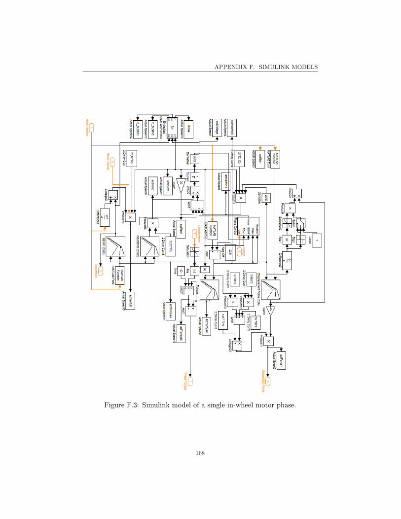
APPENDIX F. SIMULINK MODELS
Figure F.3: Simulink model of a single in-wheel motor phase.
168

APPENDIX F. SIMULINK MODELS
Figure F.4: Simulink model of an in-wheel motor phase controller.
169

APPENDIX F. SIMULINK MODELS
Figure F.5: Simulink model of the 3DOF in-wheel suspension system.
170

APPENDIX F. SIMULINK MODELS
Figure F.6: Simulink model of the 2DOF traditional suspension system.
171

APPENDIX F. SIMULINK MODELS
Figure F.7: Simulink model of the EV handling subsystem for the 3DOFsuspension.
172

APPENDIX F. SIMULINK MODELS
Figure F.8: Simulink model of the EV handling subsystem for the 2DOFsuspension.
173

Appendix G
Vehicle Handling Models
1 m curb=1000;2 m sprung=900;3 m wheel=25;4 I z=2000;5 Ixx=750; %sprung mass6
7 g=9.8;8
9 L=2.5; %wheelbase10 T track=1.4;11 T s=1.3; %spring to spring12 a=1.2; %CG to front13 b=1.3; %CG to rear14 h CG=0.6;15 h sCG=0.7;16 h RC=0.2;17
18 k tire=150000;19
20 c front=800;21 c rear=1000;22 c cornt=25000;23 c cornf=c cornt;24 c cornr=c cornt;25
26 u=20;27
28 k sbrf=0.1;29 k sbrr=0.1;30 k cbrf=1;31 k cbrr=0.1;32
33 c cambf=5000;34 c cambr=5000;35
36 roll gain=4*pi/(9.8*180); %deg/g37
38 c fsusp=800;
174

APPENDIX G. VEHICLE HANDLING MODELS
39 c rsusp=1000;40
41 hp=h sCG−h RC;42 kt=(m sprung*hp/roll gain)+(m sprung*hp*g);43 ct=0.5*((T s)ˆ2)*(c fsusp+c rsusp);44
45 %Unmodified 3DOF46
47 a3D(1,1)=−2*(c cornf+c cornr)/(m curb*u);48 a3D(2,1)=−2*(a*c cornf−b*c cornr)/(m curb*u);49 a3D(3,1)=0;50 a3D(4,1)=((2*m sprung*hp)/(m curb*Ixx*u))*(c cornf+c cornr);51
52 a3D(1,2)=−(2*(a*c cornf−b*c cornr)/(m curb*u)+u);53 a3D(2,2)=(−2)*(((aˆ2)*c cornf)+((bˆ2)*c cornr))/(I z*u);54 a3D(3,2)=0;55 a3D(4,2)=(m sprung*hp/(m curb*Ixx)) ...
*(2*(a*c cornf−b*c cornr) .../(u)+m curb*u)−(m sprung*hp*u/Ixx);
56
57 a3D(1,3)=(2/m curb)*(c cornf*k sbrf+c cornr*k sbrr ...+c cambf*k cbrf+c cambr*k cbrr);
58 a3D(2,3)=(2/I z)*(a*c cornf*k sbrf−b*c cornr*k sbrr ...+a*c cambf*k cbrf−b*c cambr*k cbrr);
59 a3D(3,3)=0;60 a3D(4,3)=((−2*m sprung*hp/(m curb*Ixx*u)) ...
*((c cornf*k sbrf) +(c cornr*k sbrr) ...+(c cambf*k cbrf)+(c cambr*k cbrr))) ...+((m sprung*g*hp−kt)/Ixx);
61
62 a3D(1,4)=0;63 a3D(2,4)=0;64 a3D(3,4)=1;65 a3D(4,4)=−ct/Ixx;66
67 b3D(1,1)=2*c cornf/m curb;68 b3D(2,1)=2*a*c cornf/I z;69 b3D(3,1)=0;70 b3D(4,1)=−m sprung*hp*c cornf/(m curb*Ixx);71
72 %Loss in Front73
74 c cornf=0;75 c cornr=c cornt;76 c cambf=0;77 c cambr=5000;78
79 a3Df(1,1)=−2*(c cornf+c cornr)/(m curb*u);80 a3Df(2,1)=−2*(a*c cornf−b*c cornr)/(m curb*u);
175

APPENDIX G. VEHICLE HANDLING MODELS
81 a3Df(3,1)=0;82 a3Df(4,1)=((2*m sprung*hp)/(m curb*Ixx*u))*(c cornf+c cornr);83
84 a3Df(1,2)=−(2*(a*c cornf−b*c cornr)/(m curb*u)+u);85 a3Df(2,2)=(−2)*(((aˆ2)*c cornf)+((bˆ2)*c cornr))/(I z*u);86 a3Df(3,2)=0;87 a3Df(4,2)=(m sprung*hp/(m curb*Ixx)) ...
*(2*(a*c cornf−b*c cornr) .../(u)+m curb*u)−(m sprung*hp*u/Ixx);
88
89 a3Df(1,3)=(2/m curb)*(c cornf*k sbrf+c cornr*k sbrr ...+c cambf*k cbrf+c cambr*k cbrr);
90 a3Df(2,3)=(2/I z)*(a*c cornf*k sbrf−b*c cornr*k sbrr ...+a*c cambf*k cbrf−b*c cambr*k cbrr);
91 a3Df(3,3)=0;92 a3Df(4,3)=((−2*m sprung*hp/(m curb*Ixx*u)) ...
*((c cornf*k sbrf) +(c cornr*k sbrr) ...+(c cambf*k cbrf)+(c cambr*k cbrr))) ...+((m sprung*g*hp−kt)/Ixx);
93
94 a3Df(1,4)=0;95 a3Df(2,4)=0;96 a3Df(3,4)=1;97 a3Df(4,4)=−ct/Ixx;98
99 b3Df(1,1)=2*c cornf/m curb;100 b3Df(2,1)=2*a*c cornf/I z;101 b3Df(3,1)=0;102 b3Df(4,1)=−m sprung*hp*c cornf/(m curb*Ixx);103
104 %Loss in Rear105
106 c cornf=c cornt;107 c cornr=0;108 c cambf=5000;109 c cambr=0;110
111 a3Dr(1,1)=−2*(c cornf+c cornr)/(m curb*u);112 a3Dr(2,1)=−2*(a*c cornf−b*c cornr)/(m curb*u);113 a3Dr(3,1)=0;114 a3Dr(4,1)=((2*m sprung*hp)/(m curb*Ixx*u))*(c cornf+c cornr);115
116 a3Dr(1,2)=−(2*(a*c cornf−b*c cornr)/(m curb*u)+u);117 a3Dr(2,2)=(−2)*(((aˆ2)*c cornf)+((bˆ2)*c cornr))/(I z*u);118 a3Dr(3,2)=0;119 a3Dr(4,2)=(m sprung*hp/(m curb*Ixx)) ...
*(2*(a*c cornf−b*c cornr) .../(u)+m curb*u)−(m sprung*hp*u/Ixx);
120
176

APPENDIX G. VEHICLE HANDLING MODELS
121 a3Dr(1,3)=(2/m curb)*(c cornf*k sbrf+c cornr*k sbrr ...+c cambf*k cbrf+c cambr*k cbrr);
122 a3Dr(2,3)=(2/I z)*(a*c cornf*k sbrf−b*c cornr*k sbrr ...+a*c cambf*k cbrf−b*c cambr*k cbrr);
123 a3Dr(3,3)=0;124 a3Dr(4,3)=((−2*m sprung*hp/(m curb*Ixx*u)) ...
*((c cornf*k sbrf) +(c cornr*k sbrr) ...+(c cambf*k cbrf)+(c cambr*k cbrr))) ...+((m sprung*g*hp−kt)/Ixx);
125
126 a3Dr(1,4)=0;127 a3Dr(2,4)=0;128 a3Dr(3,4)=1;129 a3Dr(4,4)=−ct/Ixx;130
131 b3Df(1,1)=2*c cornf/m curb;132 b3Df(2,1)=2*a*c cornf/I z;133 b3Df(3,1)=0;134 b3Df(4,1)=−m sprung*hp*c cornf/(m curb*Ixx);135
136 %Loss in Front and Rear137
138 c cornf=0;139 c cornr=0;140 c cambf=0;141 c cambr=0;142
143 a3Dfr(1,1)=−2*(c cornf+c cornr)/(m curb*u);144 a3Dfr(2,1)=−2*(a*c cornf−b*c cornr)/(m curb*u);145 a3Dfr(3,1)=0;146 a3Dfr(4,1)=((2*m sprung*hp)/(m curb*Ixx*u))*(c cornf+c cornr);147
148 a3Dfr(1,2)=−(2*(a*c cornf−b*c cornr)/(m curb*u)+u);149 a3Dfr(2,2)=(−2)*(((aˆ2)*c cornf)+((bˆ2)*c cornr))/(I z*u);150 a3Dfr(3,2)=0;151 a3Dfr(4,2)=(m sprung*hp/(m curb*Ixx)) ...
*(2*(a*c cornf−b*c cornr) .../(u)+m curb*u)−(m sprung*hp*u/Ixx);
152
153 a3Dfr(1,3)=(2/m curb)*(c cornf*k sbrf+c cornr*k sbrr ...+c cambf*k cbrf+c cambr*k cbrr);
154 a3Dfr(2,3)=(2/I z)*(a*c cornf*k sbrf−b*c cornr*k sbrr ...+a*c cambf*k cbrf−b*c cambr*k cbrr);
155 a3Dfr(3,3)=0;156 a3Dfr(4,3)=((−2*m sprung*hp/(m curb*Ixx*u)) ...
*((c cornf*k sbrf) +(c cornr*k sbrr) ...+(c cambf*k cbrf)+(c cambr*k cbrr))) ...+((m sprung*g*hp−kt)/Ixx);
157
177

APPENDIX G. VEHICLE HANDLING MODELS
158 a3Dfr(1,4)=0;159 a3Dfr(2,4)=0;160 a3Dfr(3,4)=1;161 a3Dfr(4,4)=−ct/Ixx;162
163 b3Dfr(1,1)=2*c cornf/m curb;164 b3Dfr(2,1)=2*a*c cornf/I z;165 b3Dfr(3,1)=0;166 b3Dfr(4,1)=−m sprung*hp*c cornf/(m curb*Ixx);
178