a novel decentralized voltage control method for direct current microgrids with sensitive loads

A novel decentralized voltage control method for direct currentmicrogrids with sensitive loads

Roozbeh Asad*,† and Ahad Kazemi

Center of Excellence for Power Systems Automation, Operation, Department of Electrical Engineering, Iran Universityof Science Technology, Tehran, Iran

SUMMARY

Low-voltage direct current (DC) microgrids will have a significant position in smart grids. Of course,currently, DC microgrids are mainly used in the areas with sensitive electrical loads. The main issue in thesemicrogrids is the voltage control. In this paper, a practical, reliable, modular, autonomous, and decentralizedvoltage control method, namely the voltage-based power-voltage (VbPV) control method, is proposed forthe most common type of DC microgrids, that is, the DC microgrids with sensitive loads. The proposedvoltage control method leads to the flattest voltage profile, which is essential for the DC microgrids.Besides, the presented method minimizes the power loss and maximizes the line capacity release. It isnoteworthy that the VbPV control method requires no telecommunication infrastructure. Furthermore,contrary to some other DC voltage control methods, it is applicable to different real DC microgrids. Here,some numerical examples are mentioned to discuss and clarify the remarkable achievements of the VbPVcontrol method. The analytic and simulation results confirm the successful performance of the VbPV controlmethod. Copyright © 2013 John Wiley & Sons, Ltd.

key words: decentralized voltage control; DC microgrids; DC bus signaling; voltage-power droop;distributed generation; smart grids

1. INTRODUCTION

Low-voltage direct current (DC) microgrids have promising future in smart grids. Currently, DC voltagesare internally applied by many electrical loads, especially in residential, administrative, and commercial re-gions. Some of these loads are advanced lighting systems, multimedia appliances, communication appli-ances, office supplies, home appliances equipped with drive systems, high efficiency DC (inverter) airconditioners, and electric vehicles. On the other hand, the initial output of most of growing power sources,including solar arrays, wind turbines, different micro turbines, and wave and tidal generators, is a DC volt-age or an alternating current (AC) voltage with different and sometimes varying frequencies and ampli-tudes comparing to the grid AC voltage. Also, while the application of storage systems, in parallel withrenewable sources, grows fast in electrical systems, some of the most important storage systems, such asdifferent batteries and fuel cells, inherently operate with DC voltage. Clearly, all the mentioned electricalcomponents are much more compatible with DC microgrids rather than AC microgrids [1–3]. In addition,whereas the reactive power and its control are one of the most important issues of AC microgrids, there isno reactive power in DC microgrids. In other words, the reactive power problems are completely elimi-nated at DC microgrids by the natural removal of the reactive power [4]. Considering all the earlier facts,DC microgrids will have an inevitable important position in future electrical systems, that is, smart grids.Of course, at the present time, DC microgrids are mostly applied to the regions with sensitive electricalloads including telecommunication centers and data centers [5].

*Correspondence to: Roozbeh Asad, Center of Excellence for Power Systems Automation and Operation, Department ofElectrical Engineering, Iran University of Science and Technology, Tehran, Iran.†E-mail: [email protected]

Copyright © 2013 John Wiley & Sons, Ltd.

INTERNATIONAL TRANSACTIONS ON ELECTRICAL ENERGY SYSTEMSInt. Trans. Electr. Energ. Syst. (2013)Published online in Wiley Online Library (wileyonlinelibrary.com). DOI: 10.1002/etep.1833

The voltage control is the most important issue in low-voltage DC microgrids. Because the voltage inthese microgrids is DC, no frequency and reactive power control are necessary. Furthermore, regardingthe firm correlation between active power and voltage control in DC microgrids, explained in Section 2,the active power should be regulated parallelly in the voltage control procedure.Comparing to the existing researches about the voltage control of AC microgrids and distribution sys-

tems, there are few literatures about the voltage control of DC microgrids. References [2,6–9] deal withthe voltage control of specific small DC microgrids. Also, [10] presents a voltage control method to regu-late the DC bus voltage of parallel-integrated permanent magnet wind generation systems. The voltagecontrol method is based on a master–slave hysteresis control scheme. In [11], using DC bus signaling, avoltage control method is introduced for modular photovoltaic generation systems with a battery energystorage. Besides, [12] deals with a control scheme to control different parameters, including the voltageof the terminal of DC loads, which are fed separately by different DC power sources. None of the voltagecontrol methods presented in the mentioned literatures is general and can be applied directly to the variousDC microgrids with different scales and miscellaneous DC power sources. Moreover, another voltage con-trol method presented in [13] is concentrated on only the DC loads. It is merely useful to compensate DCvoltage fluctuations in short term. In [13], no control strategy is introduced for power sources.References [14,15] introduce more general voltage control methods, but they utilize telecommunication.

Thus, the proposed voltage control methods suffer more expensive and complex implementation and lessreliability. Reference [16] presents a general voltage control method that needs no telecommunication atthe expense of the increase of complexities of the introduced voltage control method.Many researches applydroop technique [17–22] or DC bus signaling [23–25] to control the voltage ofDCmicrogrids. These generalvoltage control methods utilize the DC voltage of DC microgrids, instead of telecommunication, to do theirjob. These voltage control methods are simple, inexpensive, and reliable, but they have an important demerit.They are not compatible with the DC microgrids with considerable voltage drops [22,24,26], that is, a largeportion of real DCmicrogrids. For this reason, most of the literatures apply these voltage control methods toonly imaginary superconducting DC microgrids or small microgrids with very short electrical lines.In this paper, a practical, modular, highly reliable, and autonomous distributed voltage control method,

namely the voltage-based power-voltage (VbPV) control method, is presented for the most usual type ofDC microgrids, that is, the DC microgrids with sensitive loads. The proposed voltage control method pro-vides the flattest and approximately nominal voltage profile, which is necessary for sensitive loads, for theDCmicrogrids. Also, it is compatible with the various real microgrids containing ordinary resistive electricallines with different lengths. In Section 3, the remarkable characteristics of the proposed voltage controlmethod will be explained more.The remainder of this paper is arranged as follows. First, the principles of the DC voltage control and the

firm correlation of the voltage control and the power control in DCmicrogrids are derived. Then, the VbPVcontrol method and the proper amounts of the parameters of the voltage control method are explained. Fivenumerical examples are mentioned to discuss the capabilities of the VbPV control method more. Finally,the successful performances of the VbPV control method are verified by the simulation results.

2. PRINCIPLES OF THE VOLTAGE CONTROL IN DIRECT CURRENT MICROGRIDS

There is a firm correlation between the active power control and the voltage control in DC microgrids.At this juncture, the correlation is described in a simple DC microgrid shown in Figure 1. A T model, acapacitor, two inductors, and two resistors are considered for the line. Because the variation of thevoltage is studied in this section, the capacitors and the inductors of the lines of the DC microgridshould be considered. In fact, the capacitors and the inductors of the lines can be ignored in steady-state analyses only. The load in Figure 1 is modeled as constant power.If the voltages of the microgrid in Figure 1 are constant, the subsequent equation is valid:

ΔuC tð Þ ¼ 1C∫t

t0iC tð Þdt ¼ 0 (1)

where ΔuC(t) is the variation of the capacitor voltage between t and t0. Also, iC(t) is the consumedcurrent of the capacitor. C is the capacitance of the capacitor. Therefore,

R. ASAD AND A. KAZEMI

Copyright © 2013 John Wiley & Sons, Ltd. Int. Trans. Electr. Energ. Syst. (2013)DOI: 10.1002/etep

iC tð Þ ¼ 0 (2)

iS tð Þ ¼ iD tð Þ (3)

uD tð Þ ¼ uS tð Þ � RiD tð Þ � L diD tð Þ=dtð Þ (4)

iS(t) and iD(t) are respectively the injected current of the source and the consumed current of the load.Besides, uS(t) and uD(t) are the voltage of the source and the load, respectively. R and L arerespectively the resistance and the inductance of the electrical line. On the other hand, the consumedpower of the load, pD(t), and the generated power of the source, pS(t), are

pD tð Þ ¼ uD tð Þ iD tð Þ (5)

pS tð Þ ¼ uS tð Þ iS tð Þ (6)

Because uD(t) and pD(t) are constant, regarding Equation (5), iD(t) is constant too. Therefore,Equation (4) can be rewritten as follows:

uD tð Þ ¼ uS tð Þ � RiD tð Þ (7)

Substituting uD(t), in Equation (5), by Equation (7) gives

pD tð Þ ¼ uS tð Þ iD tð Þ � RiD2 tð Þ (8)

Considering Equations (3), (6), and (8), the generated power of the source is

pS tð Þ ¼ pD tð Þ þ ploss tð Þ (9)

where ploss(t) is the line power loss. Thus, the necessary condition for stable and constant volt-age in DC microgrids is the fulfillment of the power balance in the microgrids. Now, if thepower balance in the microgrid in Figure 1 is satisfied, in other words, if the generated poweris equal to the sum of the consumed power of the load and the electrical line power loss, thefollowing equation is valid:

pS tð Þ ¼ pD tð Þ þ ploss tð Þ (10)

Therefore,

pC tð Þ ¼ uC tð ÞiC tð Þ ¼ 0 (11)

pL tð Þ ¼ uL tð ÞiD tð Þ ¼ 0 (12)

where pC(t) and pL(t) are respectively the consumed power of the capacitor and the inductors. Besides,uL(t) is the voltage of the inductors. Regarding uC(t)≠ 0 and Equation (11),

iC tð Þ ¼ C duC tð Þ=dtð Þ ¼ 0 (13)

Consequently,

iS tð Þ ¼ iD tð Þ (14)

ΔuC tð Þ ¼ 0 (15)

Also, considering iD(t)≠ 0 and Equation (12),

uL tð Þ ¼ L diD tð Þ=dtð Þ ¼ 0 (16)

ΔiD tð Þ ¼ 0 (17)

Figure 1. A simple direct current microgrid.

A NOVEL VOLTAGE CONTROL METHOD


On the other hand,

uS tð Þ ¼ uC tð Þ þ R=2ð Þ iD tð Þ (18)

uD tð Þ ¼ uC tð Þ � R=2ð Þ iD tð Þ (19)

Therefore, according to Equations (15), (17), (18), and (19),

ΔuS tð Þ ¼ 0 (20)

ΔuD tð Þ ¼ 0 (21)

Therefore, when the power balance of a DC microgrid is fulfilled, the voltages of the microgrid willbe stable and constant. The prevenient study implies that the necessary and sufficient condition to keepthe voltage of a DC microgrid stable and constant is the continual power balance in the microgrid.Besides, it can be demonstrated that the increasing or decreasing of the voltage of DC microgridsrepresents respectively the excess or lack of the generated power in the microgrid. Thus, the voltagecontrol of DC microgrids is satisfied by the active power control. On the other hand, the DC voltagecan be utilized as the feedback signal in the procedure of the active power control.Therefore, a proper DC voltage control method must control the active power too. For this

purpose, each source must be informed the amount of power to generate by the voltage controlmethod. Some of the voltage control methods utilize telecommunication systems to inform thesources their share of power. These voltage control methods necessitate suitable telecommunica-tion infrastructures and embedded communication modules in sources. Thus, they suffer fromlow reliability and high cost. Another solution is the application of the voltage of DC microgrids[17–25]. By this solution, using a predetermined power-voltage curve for each source, all sourcesknow their exact share of power per each voltage of the DC microgrid. Therefore, no telecommu-nication is necessary. Of course, unfortunately, almost all of existing researches using the voltageof DC microgrids [17–19,22,24,25] require an approximately uniform voltage amount all aroundthe microgrid. Hence, they are only applicable in microgrids with negligible voltage drops, thatis, microgrids with superconducting conductors or very small microgrids with very short electricallines [22,24,26]. But most of DC microgrids are not very small and contain no superconductor.The voltage of each node of these microgrids is dependent on the voltage drops of the microgrids.Besides, the voltage drops are not constant. They change continuously by different occurrences,including the variations of the power consumption, the reconfiguration of the microgrid, and theoutage of sources or electrical lines. Consequently, the voltages of different nodes of themicrogrids are not the same. In fact, there is no DC voltage control method using the voltage ofmicrogrids for the ordinary DC microgrids, which are not very small and contain no superconduc-tor, that is, in the majority of DC microgrids.

3. THE VOLTAGE-BASED POWER-VOLTAGE CONTROL METHOD

Although the application of DC microgrids will promisingly develop in future, currently, DCmicrogrids are mostly applied to the regions containing sensitive loads. Obviously, the first priorityin such regions is the provision of voltage amounts with the lowest deviation from nominal voltageto the sensitive loads. This implies that the permitted voltage domain is very narrow in DC microgridswith sensitive loads, and accordingly, the voltage profile should be as flat as possible. Consequently,despite the resistive characteristics of electrical lines, the voltage that drops through the conductorshave to be minimized. Here, a practical VbPV control method is presented to provide the DCmicrogrids with sensitive loads with the flattest and approximately nominal voltage profile. The VbPVcontrol method is compatible with the various real microgrids containing ordinary resistive electricallines with different lengths. To express more clearly, the proposed voltage control method has thefollowing characteristics, which make it considerable for the DC microgrids with sensitive loads:

(1) Providing the flattest and approximately nominal voltage profile: this feature is satisfiedthrough the minimization of the inter-area voltage drops by the VbPV control method inthe whole DC microgrid.



(2) The power loss minimization and maximization of the line capacity release: Because the VbPVcontrol method minimizes the inter-area currents, the power loss minimization and the maximiza-tion of the line capacity release are the two other remarkable achievements of the proposed method.

(3) Simplicity, inexpensiveness, and high reliability: the VbPV control method benefits from anuncomplicated control system. Besides, this control method is a distributed and not centralizedcontrol method that utilizes the DC voltage of DC microgrids instead of telecommunication.These properties improve the simplicity and reliability and reduce the cost of implementationof the proposed control method impressively.

(4) Modularity and scalability: the VbPV control method intelligently and automatically adaptsitself to different types and lengths of electrical lines. In other words, different sizes of DCmicrogrids cannot disturb the success of the VbPV control method. Furthermore, in the DCmicrogrids equipped with the proposed control method, different power sources can be easilyadded, eliminated, or substituted without any necessary changes applied to the other existingpower sources.

The mentioned characteristics of the VbPV control method will be demonstrated through theanalyses and simulation results.In the proposed control method, a voltage–current curve, as shown in Figure 2, is assigned for each

source. The vertical and horizontal axes represent respectively the terminal voltage and the injectedcurrent of the source. There are five important parameters in the voltage–current curve of each source,that is, UThreshold, Kd (the droop slope), UMaxPower, Imax, and UFault. According to Figure 2, the sourcestarts generating power when its terminal voltage becomes less than the UThreshold. Decreasing theterminal voltage, the generated power of the source increases until the source reaches its maximumgenerated power (Pmax) at UMaxPower. In this operational domain, the injected current of the source,Isource, is calculated by Equation (22).

Isource ¼ UTerminal � UThresholdð ÞKd

(22)

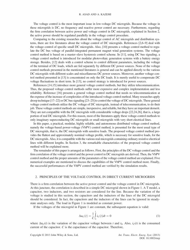
where UTerminal, Kd, and UThreshold are the terminal voltage, the droop slope, and the UThreshold of thesource, respectively. The injected current of the source remains constant and equals the maximumcurrent of the source, Imax, when the terminal voltage is between UMaxPower and UFault. If the terminalvoltage of the source becomes less than the UFault, the source is switched off. The block diagram of theVbPV control system is described in Figure 3. The simple control system is one of the merits of theVbPV control method. This makes the proposed method a reliable, inexpensive, and practical voltagecontrol method.It is noteworthy that the amount of UFault depends on the DC microgrid characteristics including the

lower limit of the permitted voltage domain and the beginning voltage of the voltage collapse.Obviously, UFault of all the sources of a DC microgrid is the same. In continuance, the proper amounts

Figure 2. The voltage–current curve of the voltage-based power-voltage control method.



of UThreshold and Kd will be discussed. Assigning the value of UThreshold and Kd of sources, UMaxPower

and Imax, as the two remaining parameters of the voltage–current curves of the sources, is determinedby the subsequent equations:

I max ¼ Pmax

UMaxPower(23)

UMaxPower ¼ UThreshold � Kd I max (24)

where Imax and Pmax are respectively the maximum current and the maximum power of the source.Also, as shown in Figure 2, UMaxPower is the terminal voltage of the source in which the source reachesits maximum current, Imax. Therefore,

U2MaxPower � UThresholdUMaxPower þ Kd Pmax ¼ 0 (25)

3.1. The proper amount of UThreshold

As mentioned before, the first priority of DC microgrids with sensitive loads is the provision of voltageamounts in the proximity of the nominal voltage to the loads. To guarantee to deliver such voltageamounts to the sensitive loads locating on the furthest nodes from the sources, the voltage–currentcurves of all the sources have to be placed as high as possible in Figure 2. Consequently, the UThreshold

of all the sources of the microgrids should be equal to the upper limit of the permitted voltage domain.

3.2. The proper amount of Kd

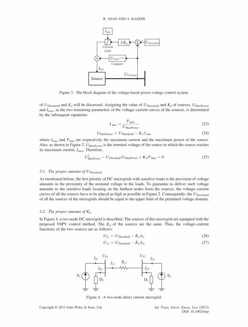
In Figure 4, a two-node DC microgrid is described. The sources of this microgrid are equipped with theproposed VbPV control method. The Kd of the sources are the same. Thus, the voltage–currentfunctions of the two sources are as follows:

US1 ¼ UThreshold � Kd IS1 (26)

US2 ¼ UThreshold � Kd IS2 (27)

Figure 3. The block diagram of the voltage-based power-voltage control system.

Figure 4. A two-node direct current microgrid.



whereUS1 andUS2 are the terminal voltage of sources 1 and 2. Also, IS1 and IS2 are the injected currentof sources 1 and 2. Combining Equations (26) and (27) gives

IS1 ¼ IS2 þUS2 � US1

Kd(28)

On the other hand,

IS1 þ IS2 ¼PD1

US1þ PD2

US2(29)

where PD1 and PD2 are the consumed powers of loads 1 and 2, respectively. If IS1, in Equation (29), issubstituted by Equation (28),

IS2 ¼12

PD1

US1þ PD2

US2

� �þ 12Kd

US1 � US2ð Þ (30)

According to Figure 4,

US1 � US2 ¼ R12I12 (31)

where R12 and I12 are the resistance and the current of the electrical line, respectively. Therefore,

IS2 ¼12

PD1

US1þ PD2

US2

� �þ 12Kd

R12I12 (32)

Similarly, the two subsequent equations are achieved:

IS1 ¼12

PD1

US1þ PD2

US2

� �� 12Kd

US1 � US2ð Þ (33)

IS1 ¼12

PD1

US1þ PD2

US2

� �� 12Kd

R12I12 (34)

Also, I12 is equal to

I12 ¼ IS1 �PD1

US1(35)

Substituting IS1 , in Equation (35), by Equation (34) gives

I12 ¼PD2US2

� PD1US1

� �

2 1þ R122Kd

� � (36)

It is noteworthy that if the electrical line of the microgrid in Figure 4 is superconductive, Equations(30), (32), (33), and (34), all can be rewritten as follows:

IS1 ¼ IS2 ¼12

PD1 þ PD2

UGrid

� �(37)

where UGrid is the voltage of the whole microgrid. Therefore, the main difference between the currentequations of the sources in superconducting microgrids and non-superconducting microgrids is thecommon second sentences of Equations (30), (32), (33), and (34).If a portion of the consumed current of an area, for instance area 1, is provided by the other one, I12

enlarges and, in conformity with Equations (32) and (34), the source of the fed area (area 1) will injectmore current comparing to the other source. As a result, more consumed current of the fed area isprovided locally, and the inter-area current, that is, I12, decreases. In other words, the proposed VbPVcontrol method causes the sources of the fed areas to oppose against and restrict the inter-area currentsby increase of their shares of the total injected current. On the other hand, as demonstrated by Equation(31), the inter-area voltage drops are directly proportional to the inter-area currents. Therefore,restricting the inter-area currents, the VbPV control method, make the inter-area voltage drops berestricted too.Generally, the distributed sources of a microgrid may feed the loads nearby the other distributed

sources, which are not full-loaded. As a result, some of the advantages of the distributed generation



are not necessarily attained perfectly. But, based on Equations (31) and (33), the loads in the DCmicrogrids with the VbPV control method are fed by the nearest distributed sources unless they arefull-loaded. Consequently, the ultimate voltage drop reduction, voltage profile improvement, powerloss reduction, lines capacity release, and transmission expansion cost reduction caused by thedistributed generation can be reached.Equations (30), (32), (33), (34), and (36) imply that the sensitivity of the sources to inter-area

currents and inter-area voltage drops can be regulated by Kd (the droop slope) of the VbPV controlmethod. Equation (36) demonstrates that if a very small value is assigned to Kd, inter-area currentsare intensively minimized and become approximately zero. Obviously, regarding Equation (31), theminimization of inter-area currents leads to the minimum inter-area voltage drops. In other words,assigning a very small value to Kd, the sensitivity of the sources to inter-area currents and inter-areavoltage drops increases largely and correspondingly; inter-area currents and inter-area voltage dropsare minimized. It is noteworthy that Kd should not be zero. The sources with zero droop slope donot tolerate even slight deviations of their terminal voltage from UThreshold. Thus, a simple voltagevariation in the DCmicrogrid causes all the sources of the DCmicrogrid to try simultaneously to eliminatethe voltage error by the ceaseless increase and decrease of their generated power. Consequently, thesources disturb the voltage control process of each other, and the DC microgrid gets unstable soon.Therefore, a very small value rather than zero is assigned to the Kd of all the sources of DC microgrids.In this manner, the proposed VbPV control method effectively minimizes the inter-area voltage dropsand currents in DC microgrids. Accordingly, the flattest and approximately nominal voltage profile isrealized in the DC microgrids with sensitive loads by the VbPV control method. Because the VbPVcontrol method minimizes the inter-area currents, the power loss minimization and the maximizationof the line capacity release are the two other remarkable achievements of the proposed control method.If a very small value is assigned to Kd, the following approximation is satisfied:

2 1þ R12

2Kd

� �≅R12

Kd(38)

Combining Equations (36) and (38) gives

I12≅Kd

R12

PD2

US2� PD1

US1

� �(39)

Equation (39) implies that in the VbPV control method, the inter-area current is inversely proportionalto R12, that is, the inter-area line resistance. That is, the proposed control method intelligently andautomatically tunes the inter-area currents inversely proportional to the line resistances or, in otherwords, lengths. In this manner, regarding Equation (31), the VbPV control method preserves theinter-area voltage drops from increasing in the long inter-area lines.It is noteworthy that all the mentioned achievements of the VbPV control method are reachable with

no telecommunication. This fact improves the simplicity and reliability and reduces the cost ofimplementation of the proposed control method impressively. Another interesting advantage of theVbPV control method is its modularity. That is, in the DC microgrids with the VbPV control method,different sources can be easily added, substituted, or eliminated without any necessary changes appliedto the other existing sources. The only point is that the newly added source should have the sameUThreshold and Kd as the other sources.Considering the earlier discussions, the VbPV control method is a practical, modular, highly

reliable, and autonomous distributed control method that provides the flattest and approximatelynominal voltage profile and minimizes the inter-area voltage drops, currents, and power loss andmaximizes the line capacity release effectively.

4. NUMERICAL EXAMPLES AND SIMULATION RESULTS

In this section, first, five numerical examples are mentioned to discuss the capabilities of the VbPVcontrol method more. Then, the successful performances of the VbPV control method are verifiedby the simulation results.



4.1. Numerical examples

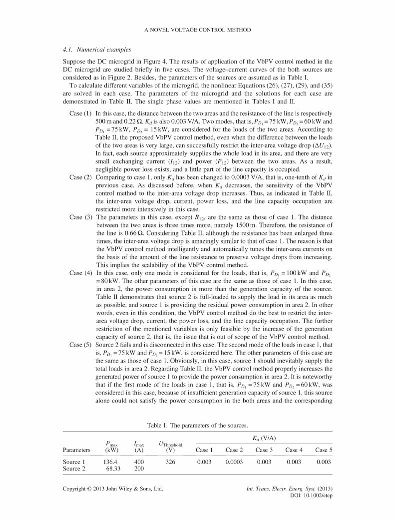
Suppose the DC microgrid in Figure 4. The results of application of the VbPV control method in theDC microgrid are studied briefly in five cases. The voltage–current curves of the both sources areconsidered as in Figure 2. Besides, the parameters of the sources are assumed as in Table I.To calculate different variables of the microgrid, the nonlinear Equations (26), (27), (29), and (35)

are solved in each case. The parameters of the microgrid and the solutions for each case aredemonstrated in Table II. The single phase values are mentioned in Tables I and II.

Case (1) In this case, the distance between the two areas and the resistance of the line is respectively500m and 0.22Ω. Kd is also 0.003V/A. Two modes, that is,PD1 = 75 kW,PD2 = 60 kW andPD1 = 75 kW, PD2 = 15 kW, are considered for the loads of the two areas. According toTable II, the proposed VbPV control method, even when the difference between the loadsof the two areas is very large, can successfully restrict the inter-area voltage drop (ΔU12).In fact, each source approximately supplies the whole load in its area, and there are verysmall exchanging current (I12) and power (P12) between the two areas. As a result,negligible power loss exists, and a little part of the line capacity is occupied.

Case (2) Comparing to case 1, only Kd has been changed to 0.0003V/A, that is, one-tenth of Kd inprevious case. As discussed before, when Kd decreases, the sensitivity of the VbPVcontrol method to the inter-area voltage drop increases. Thus, as indicated in Table II,the inter-area voltage drop, current, power loss, and the line capacity occupation arerestricted more intensively in this case.

Case (3) The parameters in this case, except R12, are the same as those of case 1. The distancebetween the two areas is three times more, namely 1500m. Therefore, the resistance ofthe line is 0.66Ω. Considering Table II, although the resistance has been enlarged threetimes, the inter-area voltage drop is amazingly similar to that of case 1. The reason is thatthe VbPV control method intelligently and automatically tunes the inter-area currents onthe basis of the amount of the line resistance to preserve voltage drops from increasing.This implies the scalability of the VbPV control method.

Case (4) In this case, only one mode is considered for the loads, that is, PD1 = 100 kW and PD2

= 80 kW. The other parameters of this case are the same as those of case 1. In this case,in area 2, the power consumption is more than the generation capacity of the source.Table II demonstrates that source 2 is full-loaded to supply the load in its area as muchas possible, and source 1 is providing the residual power consumption in area 2. In otherwords, even in this condition, the VbPV control method do the best to restrict the inter-area voltage drop, current, the power loss, and the line capacity occupation. The furtherrestriction of the mentioned variables is only feasible by the increase of the generationcapacity of source 2, that is, the issue that is out of scope of the VbPV control method.

Case (5) Source 2 fails and is disconnected in this case. The second mode of the loads in case 1, thatis, PD1 = 75 kW and PD2 = 15 kW, is considered here. The other parameters of this case arethe same as those of case 1. Obviously, in this case, source 1 should inevitably supply thetotal loads in area 2. Regarding Table II, the VbPV control method properly increases thegenerated power of source 1 to provide the power consumption in area 2. It is noteworthythat if the first mode of the loads in case 1, that is, PD1 = 75 kW and PD2 = 60 kW, wasconsidered in this case, because of insufficient generation capacity of source 1, this sourcealone could not satisfy the power consumption in the both areas and the corresponding

Table I. The parameters of the sources.

ParametersPmax(kW)

Imax(A)

UThreshold(V)

Kd (V/A)

Case 1 Case 2 Case 3 Case 4 Case 5

Source 1 136.4 400 326 0.003 0.0003 0.003 0.003 0.003Source 2 68.33 200



Table

II.The

parametersof

thedirect

currentmicrogrid

andthesolutio

nsforeach

case.

Cases

Param

eters

Solutions

Source1

Source2

The

direct

currentmicrogrid

R12(Ω

)PD1(kW)

PD2(kW)

I S(A

)US(V

)PS(kW)

I S(A

)US(V

)PS(kW)

I 12(A

)ΔU12(V

)P12(kW)

Ploss(kW)

Case1

0.22

7560

229.9360

325.310

74.800

184.976

325.445

60.199

�0.6131

�0.135

�0.199

0.00008

7515

228.0950

325.315

74.203

48.482

325.854

15.798

�2.4492

�0.538

�0.796

0.0013

Case2

0.22

7560

230.0470

325.930

74.979

184.142

325.944

60.020

�0.0625

�0.013

�0.020

0.0000008

7515

229.8590

325.931

74.918

46.264

325.986

15.081

�0.2503

�0.055

�0.081

0.000013

Case3

0.66

7560

230.3410

325.308

74.932

184.570

325.446

60.067

�0.2080

�0.137

�0.067

0.00002

7515

229.7170

325.310

74.729

46.863

325.859

15.270

�0.8311

�0.548

�0.270

0.0004

Case4

0.22

100

80363.6890

324.908

118.166

200

312.608

62.521

55.911

12.300

18.166

0.6877

Case5

0.22

7515

278.3199

325.165

90.499

——

—47.6678

10.487

15.499

0.4999



power loss. In other words, in this condition, the power balance of the DC microgrid inFigure 4 cannot be fulfilled and, as demonstrated in Section 2, the microgrid will becomeunstable. To solve this problem, the generation capacity of source 2 should increase.

4.2. Simulation results and discussions

To verify the proposed control method, the VbPV control method is applied to the low-voltage DCmicrogrid in Figure 5. The DC microgrid is an adapted version of the IEEE 34 node test feeder [27,28].In accordance with [3], the nominal voltage and the maximum permitted voltage are considered 326 and334.15V, respectively. Furthermore, the microgrid uses a two-phase (+326 V, �326V, and neutral) DCdistribution system. The resistance of the conductors is considered 0.44Ω/km. The microgrid in Figure 5includes four distributed sources and a substation connected to a transmission system by an AC–DCconverter. All the sources, including the substation, are equipped with the VbPV control method. Theirvoltage–current curves are similar to Figure 2. As mentioned in Section 3, the sources possess identicalUThreshold, Kd, and UFault. Besides, the UMaxPower and Imax of each source are calculated by Equations (23)and (25). Also, the DCmicrogrid includes sensitive constant-power two-phase loads. Themore detailed dataof the microgrid, including the branch and the load data, are presented in Tables III and IV, respectively. It isnoteworthy that the single phase values are mentioned in this section. Here, four cases are considered:

Case (1) The amounts of all the parameters of the sources in case 1 are demonstrated in Table V.Table V implies that the total installed generation capacity of the DCmicrogrid is 1005.8 kW.

Table VI demonstrates the amounts of the variables of the sources, including the generated power,the injected current, and the terminal voltage. According to Tables V and VI, source 3 is full-loaded.The reason is that the VbPV control method restricts the inter-area voltage drops and currents byautomatically forcing the sources to generate power approximately equal to the total power consump-tion of nearby loads. On the other hand, the generation capacity of source 3, which is selected in theplanning stage, is less than the total power consumption of the neighboring loads. Consequently, theVbPV control method does the best job to restrict the inter-area voltage drops as much as possible.That is, the control method forces source 3 to generate its maximum power and let the residualconsumed power of the loads be provided by the other sources. In fact, the lack of enough generatedpower in the area of source 3 inhibits the VbPV control method from presenting its entire capabilities.Despite this issue and while the total length of branches and the total two-phase load of the low-voltageDC microgrid are respectively 2056.6m and 1000.016 kW, the VbPV control method causes a propervoltage profile as shown in Figure 6. Considering Figure 6, the difference between the maximum andminimum node voltages is less than 4.2% of the nominal voltage.As stated before, to reach such a voltage profile, the VbPV control method restricts the inter-area voltage

drops and currents. Figures 7 and 8 respectively depict the voltage drops and currents of the branches of theDC microgrid. The sign of the current flowing toward node 0 is considered negative. The currents of

Figure 5. The low-voltage direct current microgrid diagram.



branches 8 and 9 are �2.36 and +0.52A, respectively. The negligible current amounts of these branchesexpectedly imply that sources 5 and 1 supply the neighboring loads merely and provide insignificant powerfor the other areas of the microgrid. Besides, the currents of branches 18 and 23 equal respectively +51.28and �387.43A. That is, sources 2 and 4, as the nearer sources to source 3, in addition to supplying theirnearby loads, expectedly compensate the power shortage in the area of source 3. As a result, the inter-areavoltage drops around source 3 increase slightly. It is interesting that source 4, as the nearest source to thearea of source 3, provides the area with much more power. Furthermore, regarding the very small current ofbranch 12, that is, �2.88 A, source 1, which is remoter to source 3 than source 2, does not supply anypower to the area of source 3. All these occurrences, which make the inter-area voltage drops remain assmall as possible, are automatically satisfied by the VbPV control method.In this case, the total generated power of the DC microgrid is 507.62 kW. Also, the total power loss

of the low-voltage DC microgrid is very small, namely 7.65 kW or 1.51% of the total generated powerof the microgrid.In fact, regarding the simulation results and the description of the VbPV control method in Section 3, in

every situation, the proposed control method does the best job in the operation stage to reach the best pos-sible voltage profile. On the other hand, the best possible voltage profile is dependent on the number, theplacement, and the capacity allocation of distributed sources, which are determined in the planning stage.In other words, the more the number of distributed sources is and the better the placement and the capacityallocation of distributed sources are done in the planning stage, the more superior is the best possiblevoltage profile, which is fulfilled by the VbPV control method in the operation stage.

Table III. The branch data of the low-voltage direct current microgrid.

Branch number From node To node Length (m)

1 0 1 17.222 1 2 11.553 2 3 215.124 3 4 38.745 3 5 250.36 5 6 198.447 6 7 0.078 7 8 2.079 8 9 11.4112 8 12 68.1510 9 10 321.3911 10 11 91.7113 12 13 20.2214 12 14 5.6115 14 15 136.4316 15 16 3.4717 16 17 155.7218 16 18 245.8319 18 19 0.0720 19 20 32.7132 19 32 021 20 21 10.8122 20 22 38.9123 22 23 13.4828 22 28 1.8724 23 24 17.8925 24 25 5.7426 24 26 1.8727 26 27 32.4429 28 29 9.0130 29 30 24.331 30 31 3.5433 32 33 70.48Total length of branches 2056.6



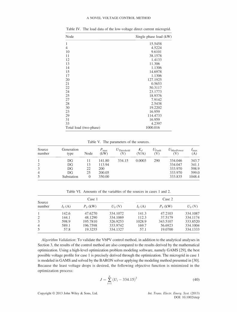
Algorithm Validation: To validate the VbPV control method, in addition to the analytical analyses inSection 3, the results of the control method are also compared to the results derived by the mathematicaloptimization. Using a high-level optimization problem modeling software, namely GAMS [29], the bestpossible voltage profile for case 1 is precisely derived through the optimization. The microgrid in case 1is modeled in GAMS and solved by the BARON solver applying the modeling method presented in [30].Because the least voltage drops is desired, the following objective function is minimized in theoptimization process:

J ¼ ∑n

i¼1Ui � 334:15ð Þ2 (40)

Table IV. The load data of the low-voltage direct current microgrid.

Node Single phase load (kW)

1 15.54584 4.522410 9.610111 38.157812 1.413313 11.30614 1.130615 14.697817 1.130620 127.192521 0.565322 50.311724 23.177325 18.937627 7.914228 2.543830 19.220223 16.95929 114.473331 16.95933 4.2397Total load (two-phase) 1000.016

Table V. The parameters of the sources.

Sourcenumber

Generationtype Node

Pmax(kW)

UThreshold(V)

Kd(V/A)

UFault(V)

UMaxPower(V)

Imax(A)

1 DG 11 141.80 334.15 0.0003 290 334.046 343.72 DG 13 113.94 334.047 341.13 DG 22 200 333.970 598.94 DG 25 200.05 333.970 599.05 Substation 0 350.00 333.835 1048.4

Table VI. Amounts of the variables of the sources in cases 1 and 2.

Sourcenumber

Case 1 Case 2

IS (A) PS (kW) US (V) IS (A) PS (kW) US (V)

1 142.6 47.6270 334.1072 141.3 47.2103 334.10872 144.1 48.1290 334.1069 112.3 37.5179 334.11743 598.9 195.7810 326.9253 1028.9 343.5107 333.85204 589.1 196.7598 333.9742 169.7 56.6923 334.10045 57.8 19.3255 334.1327 57.1 19.0700 334.1333



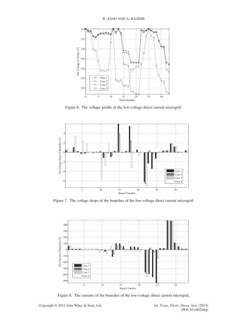
Figure 6. The voltage profile of the low-voltage direct current microgrid.

Figure 7. The voltage drops of the branches of the low-voltage direct current microgrid.

Figure 8. The currents of the branches of the low-voltage direct current microgrid.



where Ui is the voltage of node i. Also, n is the total number of the nodes of the DC microgrid. Table VIIdemonstrates the voltage of the nodes and ΔUmax in case 1 computed by the VbPV control method, andthe mathematical optimization. ΔUmax in each method is the difference between the maximum andminimum node voltages derived through the method. According to Table VII, the difference betweenthe two voltages of each node and, as a result, the voltage profiles derived by the two methods isnegligible (less than 0.12%). Moreover, the difference between ΔUmax in the two methods is0.0938%. That is, as shown analytically in Section 3, the VbPV control method could minimize thevoltage drops and, as a result, satisfy the best possible voltage profile in the DC microgrid in case 1.It is noteworthy that the VbPV control method reached such a remarkable achievement with neithercentralized heavy mathematical computations nor telecommunication.Case (2) If the generation capacity (Pmax) of source 3 is determined more than the total power

consumption of the neighboring loads, for instance 400 kW, the voltage profile ofthe DC microgrid improves as expected. In this case, Imax and UMaxPower of source3 change to 1198.4 A and 333.790V, respectively. Table VI implies that source 3 isno longer full-loaded. According to Figure 6, the difference between the maximumand minimum node voltages decreases to less than 2.21% of the nominal voltage.Also, Figures 7 and 8 show that, comparing to case 1, the inter-area voltage drops and

Table VII. The voltage of nodes and ΔUmax in case 1.

Nodenumber

The voltage of nodes (V)Difference

(%)Optimization method (GAMS) VbPV control method

0 334.1500 334.1326 0.00521 333.7126 333.6944 0.00552 333.6560 333.6372 0.00563 332.6016 332.5723 0.00884 332.3697 332.3403 0.00885 332.8733 332.8318 0.01256 333.0887 333.0376 0.01547 333.0888 333.0376 0.01548 333.0910 333.0398 0.01549 333.0882 333.0372 0.015310 333.0083 332.9636 0.013411 334.1500 334.1072 0.012812 333.1820 333.1260 0.016813 334.1500 334.1068 0.012914 332.9315 332.8717 0.018015 327.0417 326.8869 0.047316 326.9605 326.8033 0.048117 326.7234 326.5661 0.048118 321.5832 321.2570 0.101519 321.5818 321.2555 0.101520 321.0561 320.7077 0.108521 321.0477 320.6993 0.108522 327.2440 326.8752 0.112723 329.4728 329.1736 0.090824 332.8351 332.6285 0.062125 334.1500 333.9733 0.052926 332.8155 332.6089 0.062127 332.4757 332.2689 0.062228 326.8560 326.4869 0.112929 325.0166 324.6457 0.114130 323.8221 323.4500 0.114931 323.7406 323.3684 0.115032 321.5818 321.2555 0.101533 321.1729 320.8457 0.1019ΔUmax (%) 4.0191 4.1129 0.0938



currents lessen mostly. The negligible current amount of branches 8, 9, 12, and 18implies that sources 1, 2, 3, and 5 supply their nearby loads only, and insignificantpower is exchanged between the areas of the sources. Although the current of branch23 decreases to less than one-twelfth, that is, 30.98A, it still possesses a considerableamount. The reason is the very short distance between the areas of sources 3 and 4.As a result, the inter-area current between the two areas causes very small voltagedrop. For instance, the voltage drop of branch 23 is just 0.184 V in this case.Therefore, the VbPV control method wisely and automatically does not restrict theinter-area current in branch 23 further. In this case, the total generated power ofthe DC microgrid decreases to 504.00 kW. The reason is the reduction of the totalpower loss to 4.16 kW or 0.82%.

Case (3) Comparing to case 2, the distances among the areas of the sources are increased. Ten percent of the total branch length of the low-voltage DC microgrid, that is, 206m, is added tothe length of branches 8, 9, 18, and 23. In case 2, the currents of branches 8, 9, 18, and 23are respectively �3.11, 1.76, 17.9 and 30.98A. But, in this case, the currents of branches8, 9, 18, and 23 change to �2.61, 1.48, 12.58, and 4.87A, respectively. In other words, torestrict the voltage drops, the VbPV control method intelligently and automaticallydecreases the amount of inter-area currents while the inter-area resistances increase.Consequently, as depicted in Figure 6, despite the considerable increase in the distancesamong the areas of the sources, the voltage profile in this case is amazingly similar to thatof case 2. Besides, regarding Figure 6, the difference between the maximum and minimumnode voltages is 2.26%, that is, only 0.05% greater than that of case 2.

In this case, the total generated power and the total power loss of the DC microgrid are respectively504.05 and 4.20 kW (0.83%). The amounts of all the parameters of the sources in case 3 aredemonstrated in Table VIII.

Case (4) If source 2 fails and is disconnected in the DC microgrid in case 2, the amounts ofthe parameters of the other sources change as listed in Table VIII. In this case, thepower demand at the area of source 2 should be provided by the other sourcesinevitably. Comparing to case 2, sources 1, 3, and 5, as the neighboring sources tothe area of source 2, increase their generated powers by 13.88, 16.24, and 8.499 kW,respectively. In other words, after the disconnection of source 2, sources 3, 1, and 5provide respectively more power to the area of source 2. On the other hand, accordingto Figure 5 and Table III, the distances between source 2 and the three sources, that is,source 3, 1, and 5, are respectively 483.25, 512.88, and 783.14m. That is, the VbPVcontrol method wisely and automatically shares the provision of the power demand ofthe area of source 2 among the neighboring sources inversely proportional to thedistances of the sources from the area. In this manner, the VbPV control methodrestricts the inter-area voltage drops as much as possible. As a result, despite thedisconnection of source 2, the VbPV control method leads to a proper voltage profileas demonstrated in Figure 6. Figure 6 shows that the difference between the maximumand minimum node voltages is less than 3.63%.

Table VIII. Amounts of the variables of the sources in cases 3 and 4.

Sourcenumber

Case 3 Case 4

IS (A) PS (kW) US (V) IS (A) PS (kW) US (V)

1 106.1 35.4561 334.1192 182.9 61.0925 334.09522 141.6 47.3057 334.1086 — — —3 1008.2 336.6049 333.8581 1077.6 359.7461 333.82694 195.9 65.4380 334.0927 170.6 56.9872 334.09885 57.6 19.2406 334.1332 82.5 27.5685 334.1253



In this case, because the inter-area currents to the area of source 2 increases inevitably, the total powerloss of the DC microgrid is slightly greater than case 2. The VbPV control method restricts the total powerloss to 5.39 kW or 1.07%. Also, the total generated power of the DC microgrid is 505.39 kW in this case. Itis remarkable that the earlier achievements are reached with no telecommunication.

5. CONCLUSION

In this paper, a distributed voltage control method namely the VbPV control method was presented forthe most usual type of DC microgrids, that is, the DC microgrids with sensitive loads. The proposedvoltage control method is compatible with the various real microgrids containing ordinary resistiveelectrical lines with different lengths. Regarding analyses, discussions, and simulation results of thispaper, the VbPV control method effectively minimizes the inter-area voltage drops and currents inDC microgrids even when some of the sources are full-loaded. In other words, the VbPV controlmethod causes the loads in DC microgrids to be fed by the nearest distributed sources as much as pos-sible. Consequently, the advantages of distributed generation are attained perfectly by the controlmethod. Besides, the flattest and approximately nominal voltage profile is realized in the DCmicrogrids with sensitive loads by the proposed VbPV control method. It minimizes the power lossand maximizes of the line capacity release too. The VbPV control method benefits from an uncompli-cated control system. In addition, it utilizes no telecommunication. Also, applying the VbPV controlmethod to a DC microgrid, different sources can be easily added, eliminated, or substituted. Thus,the VbPV control method is a practical, simple, inexpensive, scalable, modular, highly reliable, andautonomous distributed control method.

6. LIST OF SYMBOLS AND ACRONYMS

6.1. ParametersC capacitance of the lineImax maximum current of the sourceKd droop slopeL inductance of the linePDi consumed power of load iPmax generation capacity of the sourceR resistance of the lineUFault terminal voltage of the source below which the source is switched offUMaxPower terminal voltage of the source at which the source reaches its maximum currentUThreshold terminal voltage of the source above which the source is switched off

6.2. Variables

ΔU12 voltage drop between areas 1 and 2ΔUmax difference between the maximum and minimum node voltageI12 exchanging current between areas 1 and 2iC(t) instantaneous consumed current of the line capacitoriD(t) instantaneous consumed current of the loadiS(t) instantaneous injected current of the sourceISi injected current of source iIsource injected current of the sourceP12 exchanging power between areas 1 and 2pC(t) consumed power of the line capacitorpD(t) consumed power of the loadpL(t) consumed power of the line inductors



pS(t) generated power of the sourceuC(t) voltage of the line capacitoruD(t) voltage of the loadUGrid voltage of the microgrid with superconductive electrical linesuL(t) voltage of the line inductorsUTerminal terminal voltage of the sourceuS(t) instantaneous terminal voltage of the sourceUSi terminal voltage of source i

6.3. Abbreviations

AC alternating currentD demand (load)DC direct currentDG distributed generatorS sourceSS substationVbPV voltage-based power-voltage

REFERENCES

1. Nguyen MY, Nguyen VT, Yoon YT. Three-wire network: a new distribution system approach considering bothdistributed generation and load requirements. International Transactions on Electrical Energy Systems 2013.DOI: 10.1002/etep.1749

2. Salomonsson D, Sannino A. Low-voltage dc distribution system for commercial power systems with sensitiveelectronic loads. IEEE Transactions on Power Delivery 2007; 22(3):1620–1627.

3. Sannino A, Postiglione G, Bollen MHJ. Feasibility of a dc network for commercial facilities. IEEE Transactions onIndustry Applications 2003; 39:1409–1507.

4. Asad R, Kazemi A. Quantitative analysis of power loss changes in load, generation, storage and distributionsections of different microgrids due to the dc transition. International Review of Electrical Engineering2012; 7(5):5754–5768.

5. Ton M, Fortenbery B, Tschudi EW. DC power for improved data center efficiency. Lawrence Berkeley NationalLaboratory Report 2008 [Online]. Available: http://hightech.lbl.gov/dc-powering/documents.html

6. Kurohane K, Uehara A, Senjyu T, et al. Control strategy for a distributed dc power system with renewable energy.Renewable Energy 2011; 36(1):42–49.

7. Serban E, Serban H. A control strategy for a distributed power generation microgrid application with voltage andcurrent-controlled source converter. IEEE Transactions on Power Electronics 2010; 25(12):2981–2992.

8. Salomonsson D, Söder L, Sannino A. An adaptive control system for a dc microgrid for data centers. IEEETransactions on Industry Applications 2008; 44(6):1910–1917.

9. Kakigano H, Miura Y, Ise T, Uchida R. DC micro-grid for super high quality distribution—system configurationand control of distributed generations and energy storage devices. Proceedings in 37th IEEE Power ElectronicsSpecialists Conference 2006; 3148–3154.

10. Amin MMN, Mohammed OA. DC-bus voltage control technique for parallel-integrated permanent magnet windgeneration systems. IEEE Transactions on Energy Conversion 2011; 26(4):1140–1150.

11. Sun K, Zhang L, Xing Y, Guerrero JM. A distributed control strategy based on dc bus signalling for modularphotovoltaic generation systems with battery energy storage. IEEE Transactions on Power Electronics 2011;26(10):3032–3045.

12. Balog RS, Krein PT. Bus selection in multibus dc microgrids. IEEE Transactions on Power Electronics 2011;26(3):860–867.

13. Balog RS, Weaver WW, Krein PT. The load as an energy asset in a distributed dc smartgrid architecture. IEEETransactions on Smart Grid 2012; 3(1):253–260.

14. Guerrero JM, Vasquez JC, Matas J, Vicuña LG, Castilla M. Hierarchical control of droop-controlled ac anddc microgrids—a general approach toward standardization. IEEE Transactions on Industrial Electronics2011; 58(1):158–172.

15. Cheung TK, Cheng KWE, Sutanto D, Lee YS, Ho YL. Application of ASK modulation for dc/dc converters controlin dc distribution power system. Proceedings in 1th International Conference on Power Electronics Systems andApplications 2004; 268–272.

16. Weaver WW, Krein PT. Game-theoretic control of small-scale power systems. IEEE Transactions on PowerDelivery 2009; 24(3):1560–1567.



http://hightech.lbl.gov/dc-powering/documents.html

17. Chen D, Xu L. Autonomous dc voltage control of a dc microgrid with multiple slack terminals. IEEE Transactionson Power Systems 2012; 27(4):1897–1905.

18. Xu L, Chen D. Control and operation of a dc microgrid with variable generation and energy storage. IEEETransactions on Power Delivery 2011; 26(4):2513–2522.

19. Chen J, Chen J, Chen R, Zhang X, Gong C. Decoupling control of the non-grid-connected wind power system withthe droop strategy based on a dc micro-grid.World Non-Grid-Connected Wind Power and Energy Conference 2009;1:1–6.

20. Ito Y, Zhongqing Y, Akagi H. DC microgrid based distribution power generation system. Proceedings in 4thInternational Power Electronics and Motion Control Conference 2004; 3:1740–1745.

21. Karlsson P, Svensson J. DC bus voltage control for a distributed power system. IEEE Transactions on PowerElectronics 2003; 18:1405–1412.

22. Tang W, Lasseter RH. An LVDC industrial power distribution system without central control unit. Proceedings inIEEE 31st Annual Power Electronics Specialists 2000; 2:979–984.

23. Sun X, Lian Z, Wang B, Li X. A hybrid renewable dc microgrid voltage control. Proceedings in IEEE 6thInternational Power Electronics and Motion Control Conference 2009; 725–729.

24. Schonberger J, Duke R, Round SD. DC-bus signaling: a distributed control strategy for a hybrid renewablenanogrid. IEEE Transactions on Industrial Electronics 2006; 53:1453–1460.

25. Bryan J, Duke R, Round S. Decentralized generator scheduling in a nanogrid using dc bus signaling. Proceedings inIEEE Power Engineering Society General Meeting 2004; 1:977–982.

26. Johnson BK, Lasseter RH, Alvarado FL, Adapa R. Expandable multiterminal DC systems based on voltage droop.IEEE Transactions on Power Delivery 1993; 8:1926–1932.

27. IEEE 34 Node Test Feeder. IEEE PES Distribution System Analysis Subcommittee Reports [Online]. Available:http://www.ewh.ieee.org/soc/pes/dsacom/testfeeders/feeder34.zip

28. Kersting WH. Radial distribution test feeders. Proceedings in IEEE Power Engineering Society Winter Meeting2001; 2:908–912.

29. Brooke A, Kendrick D, Meeraus A. GAMS Release 2.25, A Users Guide. GAMS Development Corporation:Washington, 1998.

30. Paudyal S, Canizares CA, Bhattacharya K. Optimal operation of distribution feeders in smart grids. IEEETransactions on Industrial Electronics 2011; 58(10):4495–4503.



http://www.ewh.ieee.org/soc/pes/dsacom/testfeeders/feeder34.zip

a novel decentralized voltage control method for direct current microgrids with sensitive loads

Documents