a novel fault-tolerant scheduling algorithm for precedence
TRANSCRIPT
Parallel Computing, vol. 32, no. 5-6, pp. 331-356, June 2006.
A Novel Fault-tolerant Scheduling Algorithm for Precedence Constrained Tasks in Real-Time Heterogeneous Systems
Xiao Qin Department of Computer Science,
New Mexico Institute of Mining and Technology, 801 Leroy Place, Socorro, New Mexico 87801-4796
http://www.cs.nmt.edu/~xqin/ [email protected]
Hong Jiang Department of Computer Science and Engineering
University of Nebraska-Lincoln Lincoln, NE 68588-0115
Address for Manuscript correspondence:
Xiao Qin Department of Computer Science, New Mexico Institute of Mining and Technology, 801 Leroy Place, Socorro, New Mexico 87801-4796 Phone: (505) 835-5902 E-mail: [email protected] http://www.cs.nmt.edu/~xqin/
1

Parallel Computing, vol. 32, no. 5-6, pp. 331-356, June 2006.
Abstract
Fault tolerance is an essential requirement for real-time systems, due to the potentially
catastrophic consequences of faults. In this paper, we investigate an efficient off-line scheduling
algorithm in which real-time tasks with precedence constraints can tolerate one processor's permanent
failure in a heterogeneous system with fully connected network. The tasks are assumed to be non-
preemptable, and each task has two copies that are scheduled on different processors and mutually
excluded in time. In the literature in recent years, the quality of a schedule has been previously
improved by allowing a backup copy to overlap with other backup copies on the same processor.
However, this approach assumes that tasks are independent of one other. To meet the needs of real-
time systems where tasks have precedence constraints, a new overlapping scheme is proposed. We
show that, given two tasks, the necessary conditions for their backup copies to safely overlap in time
with each other are, (1) their corresponding primary copies are scheduled on two different processors,
(2) they are independent tasks, and (3) the execution of their backup copies implies the failures of the
processors on which their primary copies are scheduled. For tasks with precedence constraints, the
new overlapping scheme allows the backup copy of a task to overlap with its successors’ primary
copies, thereby further reducing schedule length. Based on a proposed reliability model, tasks are
judiciously allocated to processors so as to maximize the reliability of heterogeneous systems.
Additionally, times for detecting and handling of a permanent fault are incorporated into the
scheduling scheme. We have performed experiments using synthetic workloads as well as a real
world application. Simulation results show that compared with existing scheduling algorithms in the
literature, our scheduling algorithm improves the reliability by up to 22.4% (with an average of
16.4%) and achieves an improvement in performability, a measure that combines reliability and
schedulability, by up to 421.9% (with an average of 49.3%).
Keywords: Real-time tasks, off-line scheduling, fault-tolerance, heterogeneous systems, precedence constraints, reliability, performability
1 INTRODUCTION Heterogeneous systems have been increasingly used for scientific and commercial applications,
including real-time safety-critical applications, in which the system depends not only on the results of a computation, but also on the time instants at which these results become available. Examples of such applications include aircraft control systems, transportation systems and medical electronics. To obtain high performance for real-time heterogeneous systems, scheduling algorithms play an important role. While a scheduling algorithm maps real-time tasks to processors in a system such that
2

Parallel Computing, vol. 32, no. 5-6, pp. 331-356, June 2006.
deadlines and response time requirements are met [29], the system must also guarantee its functional and timing correctness even in the presence of hardware and software faults, especially when the application is safety-critical. To address this important issue and to improve on some existing
solutions in the literature, this study investigates a scheduling algorithm with which real-time tasks with precedence constraints can be statically scheduled to tolerate the failure of one processor in a heterogeneous system.
In this paper we comprehensively address the issues of fault-tolerance, reliability, real-time, task precedence constraints, and heterogeneity. We propose an algorithm, referred to as eFRD (efficient Fault-tolerant Reliability Driven Algorithm), can tolerate one processor’s failures in a heterogeneous system with fully connected network. Failures considered in our study are of the fail-silent type, and the failures are detected after a fixed amount of time. To tolerate any one processor’s permanent failure, the algorithm uses a Primary/Backup technique [9][10][11][17][21] to allocate two copies of each task to different processors. Thus, the backup copy of a task executes if its primary copy fails due to the failure of its assigned processor. To improve the quality of the schedule, a backup copy is allowed to overlap with other backup copies on the same processor, as long as their corresponding primary copies are allocated to different processors [9][21]. As an added measure of fault-tolerance, the proposed algorithm also takes the reliability of the processors into account. Tasks are judiciously allocated to processors not only to reduce the schedule length, but also to improve the reliability as well. In addition, the time for detecting and handling of a permanent fault is incorporated into the scheduling scheme, thus making the algorithm more practical. Computational, communication and reliability heterogeneities are also taken into account in the algorithm, as explained in detail in later sections. Various algorithms studied in [1-11][13-29] share one or two features with eFRD, in terms of the assumed operational conditions, as explained in Section 2. However, eFRD is arguably the most comprehensive, in terms of the number of different scheduling issues addressed, and outperforms several quantitatively comparable algorithms in the literature. More specifically, extensive simulation studies carried out by the authors showed that the proposed algorithm significantly outperforms all three relevant and quantitatively comparable algorithms found in the literature, namely, FRCD [24], the one in [10][11], which we call FGLS (fault-tolerant greedy list scheduling), and the one in [21], called OV by the original authors of that paper.
In the section that follows, related work in the literature is briefly reviewed to present a background for the proposed algorithm and to contrast eFRD with other algorithms to show its relevance, similarity, and uniqueness. The rest of the paper is organized as follows. Section 3 presents the system characteristics and quantitatively analyzes the reliability of a heterogeneous system. Section 4 describes the eFRD algorithm and the main principles behind it, including theorems used for presenting the algorithm. Performance evaluation is given in Section 5 where three main measures
3
Parallel Computing, vol. 32, no. 5-6, pp. 331-356, June 2006.
of performance, namely, schedulability, reliability, and performability are described and used for performance assessment of eFRD in comparison with three relevant and quantitatively comparable algorithms. Finally, Section 6 concludes the paper by summarizing the main contributions of this
paper and by commenting on future directions for this work.
2 RELATED WORK Fault-tolerance must be considered in the design of scheduling algorithms, because occurrences of
faults are often unpredictable in computer systems [15][18]. Ahn et al. studied a delayed scheduling algorithm using a passive replica method [2]. Liberato et al. proposed a necessary and sufficient feasibility-check algorithm for fault-tolerant scheduling [16]. Bertossi et al. extended the well-known Rate-Monotonic First-Fit assignment algorithm. In their new algorithm, all task copies were considered by Rate-Monotonic priority order and assigned to the first processor in which they fit. Caccamo and Buttazzo developed an algorithm to schedule hybrid task sets consisting of firm and hard periodic tasks [6]. Both of the above algorithms assumed that the underlying system either is homogeneous or consists of a single processor.
Scheduling algorithms fall into two major camps: static and dynamic scheduling. Static scheduling algorithms know task sets and their constraints a priori [37]. Ramaritham proposed a static algorithm for allocating and scheduling periodic tasks running in distributed systems [37]. Dynamic scheduling algorithms heavily rely on system current sate at the time of scheduling. Therefore, it is imperative for dynamic scheduling to leverage mechanisms to collect and analyze system states, which in turn exhibit extra overheads. Static scheduling algorithms, by contrast, can make scheduling decisions in a fast and efficient way. Although static scheduling algorithms may make poor decisions in dynamic environments, static algorithms are appealing for computing environments where task sets and constraints are known beforehand.
The issue of scheduling on heterogeneous systems has been studied and reported in the literature in recent years. These studies addressed various aspects of a complicated problem. Ranaweera and Agrawal developed a scalable scheduling scheme for heterogeneous systems [25]. In [8] and [28], reliability cost, defined to be the product of processor failure rate and task execution time, was incorporated into scheduling algorithms for tasks with precedence constraints. However, these algorithms neither provide fault-tolerance nor support real-time applications.
Previous work has been done to facilitate real-time computing in heterogeneous systems. Huh et al. proposed a solution for the dynamic resource management problem in real-time heterogeneous systems. A probabilistic model for a client/server heterogeneous multimedia system was presented in [26]. These algorithms, however, also could not tolerate any permanent processor failures.
While eFRD tolerates any one processor's permanent failure, the algorithm presented in [1], also a
4
Parallel Computing, vol. 32, no. 5-6, pp. 331-356, June 2006.
real-time scheduling algorithm for tasks with precedence constraint, does not support fault-tolerance. eFRD schedules the backup copy to start after its primary copy’s scheduled execution time, thus avoiding unnecessary execution of the backup copy if the primary copy completes successfully.
Dima et al. also devised an offline real-time and fault-tolerant scheduling algorithm to handle both processor and communication link failures [7]. However, this algorithm must execute the backup copy of a task simultaneously with its primary copy.
Tasks considered in eFRD can either be confined by precedence constraints or be independent, and eFRD may be generalized to consider heterogeneous systems, where homogeneity is just a special case. Manimaran et al. [17] and Mosse et al. [9] have proposed dynamic algorithms to schedule real-time tasks with resource and fault-tolerance requirements on multiprocessor systems, but the tasks scheduled in their algorithms are independent of one another and are scheduled on-line. Martin [19] has devised an algorithm that assumed the same system and task model as in [9]. Oh and Son also studied a real-time and fault-tolerant scheduling algorithm that statically schedules a set of independent tasks, and can tolerate one processor’s permanent failure [21]. Two common features among these algorithms [9][16][18][20][21] are that (1) tasks considered are independent from one another and (2) they are designed only for homogeneous systems. Although heterogeneous systems are considered in both [28] and eFRD, the latter considers fault-tolerance and real-time tasks while the former does not consider either.
There exist excellent studies in the arena of multi-criteria scheduling [41]. Fohler studied an adaptive fault-tolerate scheduling for real-time systems [38]. Dogan and Özgüner developed matching and scheduling algorithms for heterogeneous systems. Their algorithms account for execution time and reliability of applications [39]. Dynamic scheduling algorithms, however, have no complete knowledge pertinent to task sets and constraints. Girault et al. designed a static scheduling algorithm to automatically obtain distributed and fault-tolerant schedules [40]. Assayad et al. developed heuristic scheduling algorithm for distributed embedded systems. Their algorithm takes both reliability and real-time constraints into account [41]. In addition to the issue of multi-criteria, this study is focused on a novel overlapping scheme.
Very recently, Girault et al. [10][11] have proposed a real-time scheduling algorithm (referred to as FGLS) for heterogeneous systems that considers fault-tolerance and tasks with precedence constraints. This study is by far the closest to eFRD that the authors have found in the literature. The main distinction between FGLS [10][11] and eFRD is four-fold. First, the former does not consider task deadlines explicitly, thus implying soft real-time systems, while eFRD considers hard real-time systems. Second, eFRD considers heterogeneity in computation, communication, and reliability while the former only considers computational heterogeneity. Third, the former does not consider reliability when scheduling tasks while eFRD is reliability-driven. Forth, the former allows the concurrent
5
Parallel Computing, vol. 32, no. 5-6, pp. 331-356, June 2006.
execution of primary and backup copies of a task while eFRD allows backup copies of tasks whose primary copies are scheduled on different processors to overlap one another. Last, FGLS handles several failures, whereas eFRD tolerates only one processor’s failure at a time.
In the authors’ previous work, both static [23][24] and dynamic [22] real-time scheduling schemes for heterogeneous systems were developed. One similarity among these algorithms is that the Reliability Driven Scheme is applied to the algorithms to enhance the reliability of the heterogeneous systems. With the exception of the FRCD (Fault-tolerant Reliability Cost Driven) algorithm [24], other algorithms proposed in [22] and [23] cannot tolerate any failure. In this paper, the FRCD algorithm [24] is extended by relaxing the requirement that backup copies of tasks be prohibited to overlap with one another.
3 SYSTEM MODEL FOR RELIABILITY 3.1. System Model
In parallel and systems, real-time jobs with dependent tasks can be modelled by Directed Acyclic Graphs (DAGs). In this paper, a DAG is defined as T = {V, E}, where V = {v1, v2,...,vn} represents a set of real-time tasks that are assumed to be non-preemptable, and a set of weighted and directed edges E represents communication among tasks. (vi, vj)∈ E indicates a message transmitted from task vi to vj.
When one processor in a system fails, it takes a certain amount of time, denoted δ, to detect and handle the fault. To tolerate permanent faults in one processor, a primary-backup (PB) technique is applied in the proposed scheduling scheme. Thus, two copies of any task, denoted vP and vB, are executed sequentially on two different processors. Without loss of generality, we assume that primary and backup copies of a task are identical. It is worth noting that the proposed approach can also be used tolerate transient processor failures, because it is sufficient to deal with transient failures using the same fault-tolerant mechanism.
A heterogeneous system considered in this study consists of a set P = {p1, p2,..., pm} of heterogeneous processors connected by a network. The network in our model provides full connectivity through either a physical link or a virtual link. This assumption is arguably reasonable for modern interconnection networks (e.g. Myrinet [35] and InfiniBand [36]) that are commonly used in heterogeneous systems. A processor communicates with other processors through message passing, and the communication time between two tasks assigned to the same processor is assumed to be zero. Note that the aspect of fault tolerance in networks is out the scope of this study.
A measure of computational heterogeneity is modeled by a function, C:V×P→Z+, which represents the execution time of each task on each processor in the system. Thus, cij denotes the execution time of task vi on processor pj. A measure of communication heterogeneity is modeled by a function Γ: E×P×P→ Z+. Communication time for sending a message (vi, vj) ∈ E from task vi on pk to task vj on
6

Parallel Computing, vol. 32, no. 5-6, pp. 331-356, June 2006.
pb is determined by wkb × eij, where eij is the volume of data and wkb is the weight on the edge between pk and pb, with wkb representing the delay involved in transmitting a message of unit length between the two processors. Given a task vi ∈ V, di, si and fi denote the deadline, scheduled start time, and
finish time (fi = si + cij) of vi’s primary copy, whereas diB, si
B and fiB (fi
B = si
B + cij) represent those of vi’s backup copy, respectively. p(vi) denotes the processor to which vi is allocated. These parameters are subject to constraints: (1) si ≤ di - cij, where p(vi
P) = j, and (2) siB
≤ diB
- cik, where p(viB) = k. A
real-time job has a feasible schedule if for all v ∈ V, the above two constraints are satisfied. Let X be an m by n binary matrix corresponding to a schedule, in which the primary copies of n
tasks are assigned to m processors. Element xij equals 1 if and only if vi’s primary copy has been assigned to processor pj; otherwise xij = 0. Likewise, let XB denote an m by n binary allocation matrix of backup copies, in which an element xB
ij is 1 if and only if the backup copy of vi has been assigned to pj; otherwise xB
ij equals 0. Therefore, we have and . 1)( =⇔= ijPi xjvp 1)( =⇔= B
ijBi xjvp
EXAMPLE 1. Fig. 1 shows a task graph that consists of 6 tasks and a system with three processors. Two allocation matrices, X for primary copies and BX for backup copies, are given below. Note that cij can be estimated by code profiling and statistical prediction [34]. p1 p2 p3 p1 p2 p3 0 1 0 v1 0 0 1 v1 1 0 0 v2 0 0 1 v2
X = 0 0 1 v3 BX = 1 0 0 v3 1 0 0 v4 0 0 1 v4 0 1 0 v5 0 0 1 v5 0 0 1 v6 1 0 0 v6
((20,8,10),55)
((10,22,7),70)((6,18,8),72)
((9,12,10),80)
((12,24,10),115)
e12 = 2 v1
v2 v3
v4 v5
e56 = 1
e36 = 1
e46 = 2
e24 = 1 e25 = 2
e15 = 1
((12,8,10),75) w23 = w32=3
w13 = w31=3 w12 = w21= 1
e13 = 2
p3 p2
p1
v6
Fig. 1 DAG task graph. Assume a 3-processor system and each real-time task is denoted byvi = ((ci1, ci2, ci3,), di), where cij is the execution time of vi on pj, and di is the deadline. eij and wij
depict data volume and communication weight, respectively. 1 ≤ i ≤ 6, 1 ≤ j ≤ 3.
3.2. Reliability Analysis
7

Parallel Computing, vol. 32, no. 5-6, pp. 331-356, June 2006.
Since many of the real-time systems operate in environments that are non-deterministic and even hazardous, it is necessary and important for systems to be fault-tolerant. To quantitatively evaluate the system’s level of fault-tolerance, a reliability model needs to be addressed, assuming that fault
arrival rate is constant and the distribution of the fault-count for any fixed time interval is approximated using a Poisson probability distribution [12][27][28]. It is to be noted that the reliability function, derived below, helps in evaluating the performance of our scheduling in Section 5.
Though the derivation of reliability is similar to that of the reliability function presented in [12][27][28], we relax one unrealistic assumption imposed on the reliability models in [12][27][28]. The models in [12][27][28] assume that the processors in a system are fault-free, implying that the reliability of the system when one processor fails is not considered. A major reason behind this assumption is that these models do not tolerate processor failures. To further enhance the reliability of the real-time system, we propose a model, on which the proposed eFRD algorithm is based.
A k-timely-fault-tolerant (k-TFT) schedule [21] is defined as the schedule in which no task deadlines are missed, despite k arbitrary processor failures. In this paper, the scheduling goal is to achieve 1-TFT for processor failure by incorporating processor and task redundancy into the scheduling algorithm.
The reliability of a processor in time interval t is ip )exp( tiλ− , where iλ (1 ≤ i ≤ m) is 's failure rate in a vector of failure rates Λ= (λ
ip1, λ2, …, λm), with m being the number of processors in the
system [27]. Likewise, the reliability of a link between pi and pj during the time interval t is )exp( tijµ− , where ijµ is an element of Μ, an m by m matrix of failure rates for links. A processor
might fail during an idle time, but it is assumed that processors’ failures during an idle time interval are not considered in our reliability model. The reason for this assumption is two-fold [12][27][28]. First, instead of affecting the system reliability, failures during an idle time merely affect the completion time of tasks. Second, a processor’s failure during an idle period can be fixed by replacing the failed processor with a spare unit, meaning that such failures are not critical for reliability analysis.
The state of the system is represented by a random variable K which takes value in {0, 1, 2, …, m}. More precisely, K = 0 means that no processor permanently fails, and K = i (1 ≤ i ≤ m) signifies that the ith processor encounters permanent failures. The probability for K is determined by equation (1), where iτ is the schedule length of processor i, or in other words, the latest of finish times among all primary copies of tasks assigned to processor i,
Pr[K = k] =
for k = 0 (1)
[ ]∏≠=
−−−m
kiiiikk
,1
)exp()exp(1 τλτλ
∏=
−m
iii
1
)exp( τλ
otherwise
8
Parallel Computing, vol. 32, no. 5-6, pp. 331-356, June 2006.
It should be noted that the notion of reliability heterogeneity is implied in the variation of computation time and failure rate. Let R(Λ, Μ, X, XB, T) denote the system reliability for a given schedule X and XB, a set Λ of processors’ failure rates, a matrix Μ of failure rates for links, and a job
T. The system reliability equals the probability that all tasks can be successfully completed even in the presence of one processor’s hardware and software faults. Under the assumption that no more
than one processor permanently fails in the current system, that is, ∑ , it calls for the
derivations of two kinds of reliabilities, namely: (1) , the reliability when every processor is operational, and (2) the reliability when exactly the kth
processor fails. Thus, the system reliability R(Λ,Μ, X, X
=
==m
iik
01)Pr(
),,,(0 TXR ΜΛ,0),,,,,( ≠ΜΛ kTXXR Bk
B, T) can be expressed as below:
[ ]∑=
ΜΛ×=+ΜΛ×==ΜΛm
k
BkB TXXRkKTXRKTXXR1
0 ),,,,()Pr(),,,()0Pr(),,,,( , (2)
where is a product of processor reliability and link reliability . Hence, the system reliability when the kth processor fails can be
written as:
),,,,( TXXR Bk ΜΛ ),,,( TXXR BkPN Λ
),,,( TXXR BkLINK Μ
. (3) mkTXXRTXXRTXXR BkLINK
BkPN
Bk ≤≤Μ×Λ=ΜΛ 0),,,,(),,,(),,,,(
Before proceeding to derive the expression of the link reliability, we first consider the expressions for two reliability functions and , which are defined to be the
product of all processors' reliabilities. Since the reliability of each processor p
),,,(0 TXXR BPN Λ ),,,( TXXR Bk
PN Λ
j can be evaluated as:
, 1 ≤ j ≤ m, the reliability and are then determined by Equation (4) and (5) ∏=
−n
iijijj cx
1
)exp( λ 0PNR k
PNR
as follows,
∏∏= =
−=Λm
j
n
iijijjPN cxTXR
1 1
0 )exp(),,( λ , (4)
⎭⎬⎫
⎩⎨⎧
−×⎭⎬⎫
⎩⎨⎧
−=Λ ∏ ∏∏ ∏≠= =≠= =
m
kjj
n
iij
Bijikj
m
kjj
n
iijijj
BkPN cxxcxTXXR
,1 1,1 1
)exp()exp(),,,( λλ
[ ]∏ ∏≠= =
−×−=m
kjj
n
iij
Bijikjijijj cxxcx
,1 1
)exp()exp( λλ
[ ]∏ ∏≠= =
+−=m
kjj
n
i
Bijikijijj xxxc
,1 1
)(exp λ , where 1 ≤ k ≤ m. (5)
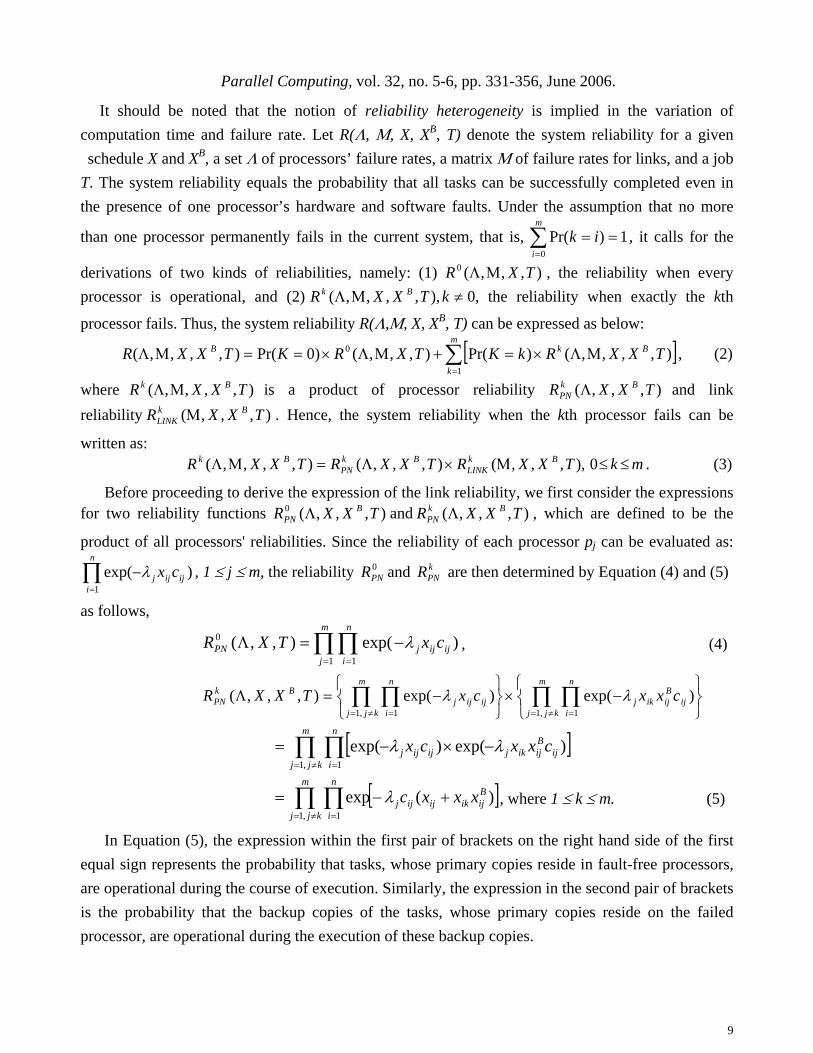
In Equation (5), the expression within the first pair of brackets on the right hand side of the first equal sign represents the probability that tasks, whose primary copies reside in fault-free processors, are operational during the course of execution. Similarly, the expression in the second pair of brackets is the probability that the backup copies of the tasks, whose primary copies reside on the failed processor, are operational during the execution of these backup copies.
9

Parallel Computing, vol. 32, no. 5-6, pp. 331-356, June 2006.
EXAMPLE 2. Consider the task and processor graphs shown in Figure 1 as an example, where the schedule result is represented by X and XB illustrated in Example 1. Thus, we have: 1635241332112 ====== xxxxxx , , and, 1615343312313 ====== BBBBBB xxxxxx
( ) ( ) ( ))(exp)(exp)(exp),,( 6333352122412110 ccccccTXRPN +−×+−×+−=Λ λλλ ,
( ) ( ))(exp)(exp),,,( 432363333521221 ccccccTXXR BPN +++−×+−=Λ λλ ,
( ) ( ))(exp)(exp),,,( 531363333412112 ccccccTXXR BPN +++−×+−=Λ λλ ,
( ) ( ))(exp)(exp),,,( 521226131412113 ccccccTXXR BPN +−×+++−=Λ λλ .
Before determining , a link reliability when every processor is operational, we derive a probability that the link between p
),,(0 TXRLINK Μ),,( TXRkb Μ k and pb is operational during the transmission
of messages through this link. The set of all messages transmitted from pk to pb is defined as below: { }110),( =∧=∧>= jbikijjikb xxevvE , ∀1 ≤ k, b, q ≤ m: k ≠ b, k ≠ q, and b ≠ q.
where eij > 0 signifies that a message is sent from vi to vj, xik = 1 means that the primary copy of vi is assigned to pk, and xjb = 1 indicates that the primary copy of vj is assigned to pb. The reliability of the message (vi, vj) ∈ Ekb is the probability that the link connecting pk and pb is operational during the time interval when the message is being transmitted. Hence, message (vijkbew i, vj)’s reliability can be calculated as: )exp( ijkbjbikkb ewxxµ− )exp( ijkbkb ewµ−= . Based on the definition of message reliability, ),,( TXRkb Μ can be expressed as the product of the reliabilities of all messages that belong to set Ekb. More precisely, ),,( TXRkb Μ is obtained as:
[ ]∏ ∏ ∏= ≠= ∈
−=−=Μn
i
n
ijj Evvijkbkbijkbjbikkbkb
kbj
ewewxxTXR1 ,1 ),( ,
)exp()(exp),,( µµ . (6)
) is determined as a product of all links’ reliabilities, and therefore we have, ,,(0 TXRLINK Μ
∏ ∏= ≠=
Μ=Μm
k
m
kbbkbLINK TXRTXR
1 ,1
0 ),,(),,( . (7)
EXAMPLE 3. Again, given a heterogenous system illustrated in Example 1, where ,12112 == ww and , we have 33113 == ww 33223 == ww === 1321215212 )},,{()},,{( EvvEvvE ),,{()},,{( 312364 vvEvv =
and, . )},( 65 vv ( ))(3exp)3exp()exp()exp(),,( 5613234613122125120 eeeeeTXRLINK +−×−×−×−=Μ µµµµ
Similar to the reliability function of calls for the derivation of link reliability , which is a probability that the link between p
0LINKR , q
LINKR),,( TXRq
kb Μ k and pb is operational when exactly the qth processor fails under a schedule X. Before proceeding to derive the expression of , we
define two sets of messages that have to be transmitted if p
),,( TXRqkb Μ
q encounters permament failures: { }1110),( =∧=∧=∧>= B
jbjqikijjiqkb xxxevvE ,
{ }11110),( =∧=∧=∧=∧>=′ Bjbjq
Bikiqijji
qkb xxxxevvE ,
∀1 ≤ k, b, q ≤ m: k ≠ b, k ≠ q, and b ≠ q. qkbE implies that, if , the primary copy of vq
kbji Evv ∈),( i is assigned to pk, the primary and backup
10

Parallel Computing, vol. 32, no. 5-6, pp. 331-356, June 2006.
copies of vj are assigned to pq and pb respectively, then this message must be shipped from vi’s primary copy to vj’s backup copy due to pq’s failure. Similarly, indicates that, if ,
the primary copies of v
qkbE ′ q
kbji Evv ′∈),(
i and vj are both assigned to pq, whereas the backup copies of vi and vj are assigned to pk and pb, respectively, forcing the message to be sent from the backup copy of vi to that of vj (i.e., through the link between pk and pb).
Thus, is defined to be a product of the reliabilities of all messages that belong to
the three message sets: E
),,,( TXXR Bqkb Μ
kb, , and . Therefore, we have: qkbE q
kbE′
[ ]∏ ∏= ≠=
×−=Μn
i
n
ijjijkbjbikkb
Bqkb ewxxTXXR
1 ,1
)(exp),,,( µ
[ ] ×⎭⎬⎫
⎩⎨⎧
−∏ ∏= ≠=
n
i
n
ijjijkb
Bjbjqikkb ewxxx
1 ,1
))((exp µ
[ ]⎭⎬⎫
⎩⎨⎧
−∏ ∏= ≠=
n
i
n
ijjijkb
Bjbjq
Bikiqkb ewxxxx
1 ,1
))()((exp µ
∏∏∏′∈∈∈
−×−×−=q
kbjiqkbjikbji Evv
ijkbkbEvv
ijkbkbEvv
ijkbkb ewewew),(),(),(
)exp()exp()exp( µµµ . (8)
Since denotes the reliability of all links when processor p),,,( TXXR BqLINK Μ q encounters
permanent failures, it can be written as the following expression:
. (9) ∏ ∏≠= ≠≠=
Μ=Μm
qkk
m
qbkbb
Bqkb
BqLINK TXXRTXXR
,1 ,,1
),,,(),,,(
EXAMPLE 4. Consider again the system from Example 1, and suppose p1 is not operational. We
have , ∏ ∏≠= ≠≠=
×Μ=Μ=Μ3
1,1
3
1,,1
123
11 ),,,(),,,(),,,(kk bkbb
BBkb
BLINK TXXRTXXRTXXR ),,,(1
32 TXXR BΜ
)},(),,{( 653123 vvvvE = , and)},,(),,{( 5121132 vvvvE = =′===′ 1
3213232
123 EEEE ∅ . Thus,
. Similary, we have ( ))(3exp),,,( 15125613231 eeeeTXXRLINK +++−=′Μ µ == 212112 )},,{( EvvE
. Hence, )},,{( 52 vv )},(),,{()},,{( 65313316413 vvvvEvvE ==
( ) ( )(3exp3exp),,,(),,,(),,,( 5613314613231
213
2 eeeTXXRTXXRTXXR BBBLINK +−×−=Μ×Μ=Μ µµ ) , and
( ) ( 25211212221
312
3 expexp),,,(),,,(),,,( eeTXXRTXXRTXXR BBBLINK µµ −×−=Μ×Μ=Μ ).
We are now in a position to derive the expression for the system reliability R(Λ, Μ, X, XB, T) by substituting (4), (5), (7) and (9) into (2). Thus, the system reliability can be caculated as:
+⎥⎦
⎤⎢⎣
⎡Μ⎥
⎦
⎤⎢⎣
⎡−×==ΜΛ ∏ ∏∏∏
= ≠== =
m
k
n
kbbkb
m
jijij
n
ij
B TXRcxKTXXR1 ,11 1
),,()exp()0Pr(),,,,( λ
. (10) ∑ ∏ ∏∏ ∏= ≠= ≠≠=≠= ⎪⎭
⎪⎬⎫
⎪⎩
⎪⎨⎧
⎥⎦
⎤⎢⎣
⎡Μ⎥
⎦
⎤⎢⎣
⎡+−×=
m
q
m
qkk
m
qbkbb
Bqkb
m
kjj
n
i
Bijikijijj TXXRxxxcqK
1 ,1 ,,1,1
),,,()(exp()Pr( λ
11

Parallel Computing, vol. 32, no. 5-6, pp. 331-356, June 2006.
4 SCHEDULING ALGORITHMS
In this section, we present eFRD, an efficient fault-tolerant, reliability-cost driven scheduling algorithm for real-time tasks with precedence constraints in a heterogeneous system.
This algorithm schedules real-time jobs with dependent tasks at compile time, by allocating primary and backup copies of tasks to processors in such a way that: (1) Total schedule length is reduced so that more tasks can complete before their deadlines; (2) Permanent failures in one processor can be tolerated; and (3) The system reliability is enhanced by assigning tasks to processors that provide high reliability.
4.1 An Outline It is assumed in the system model (Section 3) that at most one processor encounters permanent
failures. The key for tolerating permanent failures in a single processor is to allocate the primary and backup copies of a task to two different processors such that the backup copy subsequently executes if the primary copy fails to complete. This approach referred to as Primary/Backup technique has been extensively studied in the literature [9,10,21]. The Primary/Backup techniques presented in [9][10][21] are developed for real-time systems where tasks are independent from one another, meaning that there are no precedence constraints and the backup copy of a task executes if and only if its primary copy fails. However, the above condition for backup copies’ execution has to be extended to meet the needs of tasks with precedence constraints. More precisely, given a task vj, then there are two cases in which vj
P may fail to execute: (1) a fault occurs on p(vjP) before time finish fj, and (2)
p(vjP) is operational before fj, but vj
P fails to receive messages from all its predecessors. Case (2) is illustrated by a simple example in Fig. 2 where dotted lines denote messages sent from predecessors to successors. Let vi be a predecessor of vj, and p(vi) ≠ p(vj). Suppose p(vi
P) fails before fi, then viB
should execute. Since vjP cannot receive a message from vi
B, vjP still can not execute even if p(vj
P) is operational. The primary copy of a task that never encounters case (2) is referred to as a strong primary copy, as formally defined in Def. 1. Thus, a task v has a strong primary if the primary and backup tasks of all v’s predecessors are scheduled to finish earlier than the start time of vP (accounting for communication time) and thus the vP can receive all the messages of its predecessors.
DEFINITION 1. Given a task v, vP is a strong primary copy, if and only if the execution of vB implies the failure of p(vP) before time f.
It is of critical importance to determine whether a task has a strong primary copy. It is straightforward to prove that a task without any predecessor has a strong primary copy. Based on this
viB
vjP
vjB
viP
Fig. 2 Since processor p1 fails, viB executes.
Because vjP can not receive message from vi
B,vj
B must execute instead of vjP.
time
p3
p2
p4
p1
12

Parallel Computing, vol. 32, no. 5-6, pp. 331-356, June 2006.
fact, Theorem 1, below, suggests an approach to determine whether a task with predecessors has a strong primary copy. In this approach, we assume that we already know if all the predecessors have strong primary copies or not. By using this approach recursively, starting from tasks with no
predecessors, we are able to determine whether a given task has a strong primary copy. To facilitate the description and proof of Theorem 1-5, which are used in the eFRD algorithm, we need to further introduce the following definitions. DEFINITION 2. vi is schedule-preceding vj, if and only if sj ≥ fi. DEFINITION 3. vi is message-preceding vj, if and only if vi sends a message to vj. Note that vi is message-preceding vj implies that vi is schedule-preceding vj, but not inversely. DEFINITION 4. vi is execution-preceding vj, if and only if both tasks execute and vi is message-preceding vj. Note that vi is execution-preceding vj implies that vi is both message-preceding and schedule-preceding vj, but not inversely. THEOREM 1. (a) A task with no predecessors has a strong primary copy. (b) Given a task vi and any of its predecessors vj , if they are allocated to the same processor and vj has a strong primary copy, or, if they are allocated on two different processors and the backup copy of vj is schedule-preceding the primary copy of vi , then vi has a strong primary copy. That is, ∀vj∈V, (vj, vi) ∈ E’: ((p(vi
P) = p(vjP) ∧
(vjP
is a strong primary copy)) ∨ (p(viP) ≠ p(vj
P) ∧ (vjB is message-preceding vi
P)) ⇒ (viP is a strong
primary copy). PROOF. As the proof of (a) is straightforward from the definition, it is omitted here. We only prove (b). Suppose p(vi
P) is operational before fi. There are two possibilities: (1) p(viP) = p(vj
P), we have fj < fi, implying that p(vj
P) does not fail before fj. Because vjP is a strong primary copy, vj
P must execute. (2) p(vi
P) ≠ p(vjP) and vj
B is message-preceding viP , implying that even if one processor fails, vi
P can still receive message from task vj. Based on (1) and (2), we have proven that vi
P can receive messages from all its predecessors. In other words, vi
P must execute since p(vjP) is operational by time fi.
Therefore, according to Definition 1, viP is a strong primary copy. �
In the eFRD algorithm, if the backup copies of task vi and vj are allowed to overlap with each other on the same processor, then three conditions are held, namely, (1) the corresponding primary copies are allocated to the different processors; (2) vi and vj are independent with each other; and (3) the primary copies of vi and vj are strong primary copies. This argument is formally described as the following proposition, Proposition 1. ( ) ( ) ( )( ) ⇒<≤∨<≤∧=∈∀ B
jBi
Bj
Bi
Bj
Bi
Bj
Biji fssfssvpvpVvv )()(:, ∧≠ )()( P
jPi vpvp
copyprimarystrongaisvcopyprimarystrongaisvEvvEvv Pj
Piijji ∧∧′∉∧′∉ ),(),( , where E ′ is a
set of precedence constraints, which is defined as: given two tasks and , then iv jv Evv ji ′∈),( if and only if: (1) , or (2) there exists a task , such that and Evv ji ∈),( kv Evv ki ′∈),( Evv jk ′∈),( . Therefore, and are independent (or concurrent), if and only if neither iv jv Evv ji ′∉),( , nor
13

Parallel Computing, vol. 32, no. 5-6, pp. 331-356, June 2006.
Evv ij ′∉),(
14
.
Fig. 3 shows an example illustrating this case. In this example, we assume that vi and vj are independent, vi
P and vjP are strong primary copies, and vi and vj, are allocated to p1 and p3,
respectively. The two backup copies of these two tasks can be overlapped with each other on p2 because at most one of them will ever execute in the single-processor failure model.
However, if vi and vj in the above example are dependent upon one another, the overlapping between vi
B and vjB will be prohibited. More strictly, even though vi
B and vjB are scheduled on
different processors, they still are not allowed to overlap in time with each other. This statement is formalized in Proposition 2.
PROPOSITION 2. If vi and vj are dependent upon one another, the overlapping between viB and vj
B are prohibited. Thus, ( ) ( )B
jBi
Bj
Bi
Bj
Bijiji fssfssEvvVvv <≤¬∧<≤¬⇒′∈∈∀ ),(:, .
PROOF. Assume and can be overlapped in time with one another, which means will not
execute if begins running, because the message cannot be transferred from to . If a fault
occurs on before , has to execute, implying that will not execute. Neither can
successfully execute, since it is incapable of obtaining the message from either or . Therefore, task is unable to be successfully completed. This means that the assumption is incorrect, which
completes the proof for this proposition. �
Biv B
jv Bjv
Biv B
iv Bjv
)( Pivp if B
iv Bjv P
jvPiv B
iv
iv
The above proposition shows that the positive effects yielded from the backup-overlapping scheme (BOV) are lessened by the vast majority of tasks that have precedence constraints. To eliminate this limitation, we propose an alternative overlapping scheme for tasks with precedence constraints. The overlapping scheme is formally presented as Proposition 3 (Fig. 4 shows this scenario). Please note that the backup of vj should not be scheduled on p1, and the proof can be found in Theorem 3. Proposition 3. Given two tasks and , if iv jv Evv ji ′∈),( , then vi
B and vjP are allowed to overlap with
each other on the same processor. Thus, ⇒′∈∈∀ EvvVvv jiji ),(:, B
iv and are allowed to overlap with each other on the same processor. Pjv
PROOF. This argument is proved by considering the following three cases in which a failure occurs: (1) p1 has failed before . In this case, vif i
B and vjB will be guaranteed to complete on p2 and p3,
viP
vjP
vjBvj
B
time
overlap p3
p2
p1
Fig. 3 Primary copies of vi and vj are allocated top1 and p3, respectively, and backup copies of viand vj are both allocated to p2. These two backupcopies can be overlapped with each other.
p1
p2
p3
viBvj
P
vjB
overlap
timeviP
Fig. 4 (vi, vj) ∈ E’, then viB and vj
P are allowedto overlap with each other on the sameprocessor.

Parallel Computing, vol. 32, no. 5-6, pp. 331-356, June 2006.
respectively. (2) A fault occurs on p2 before . In this case, vjf iP and vj
B will successfully execute on
p1 and p3, respectively. (3) A fault occurs on p3 at an arbitrary time. In this case, the failure of p3 presents no adverse effects on vi
P and vjP, which will be successfully executing on p1 and p2. All
cases ensure that at most one of viB and vj
P will execute in the presence of a fault, implying that these two copies can be overlapped with each other on the same processor. �
The algorithm schedules tasks in the following three main steps. First, real-time tasks are ordered by their deadlines in non-decreasing order, such that tasks with tighter deadlines have higher priorities. Second, the primary copies are scheduled to satisfy the precedence constraints, to reduce the schedule length, and to improve the overall reliability. Finally, the backup copies are scheduled in a similar manner as the primary copies, except that they may be overlapped on the same processors to further reduce schedule length. More specifically, in the second and third steps, the scheduling of each task must satisfy the following three conditions: (1) its deadline should be met; (2) the processor allocation should lead to the maximum increase in overall reliability among all processors satisfying condition (1); and (3) it should be able to receive messages from all its predecessors. In addition to these conditions, each backup copy has two extra conditions to satisfy, namely, (i) it is allocated on the processor that is different than the one assigned for its primary copy, and (ii) it is allowed to overlap with other backup copies on the same processor if their primary copies are allocated to different processors. Condition (i) and (ii) can also be formally described by Proposition 4, where δ is the fault detection time measured by the time interval between the moment a failure occurs and the moment the failure is detected. Individual processor’s failure can be detected by various mechanisms including adoption of suitable self-checking [32] and periodic testing [33].
PROPOSITION 4. A schedule is 1-TFT → ( ) ( )δ+≥∧≠∈∀ iBi
BPi fsvpvpVv )()(: ∧ vi
B can overlap with other backup copies on the same processor if their primary copies are allocated to different processors.
Table 1. Definitions of Notation NOTATION DEFINITION D(v) Set of predecessors of task v. D(v) = {vi | (vi, v) ∈ E} S(v) Set of successors of task v, S(v) = {vi | (v, vi) ∈ E} F(v) Set of feasible processors to which vB can be allocated, determined in part by Theorem 3. B(v) Set of predecessors of v’s backup copy, determined by Expression (14). VQi VQi = {v1, v2, …, vq} is a queue in which all tasks are scheduled to pi, sq+1 = ∞, and f0 = 0 VQi’(v) Queue in which all tasks are scheduled to pi, and cannot overlap with the backup copy of task v,
where sq+1 = ∞, and f0 = 0 EATi(v, vj) Earliest available time for the primary or backup copy of task v if message e sent from vj∈ D(v)
represents the only precedence constraint. EATi
P(v) Earliest EATi time of v’s primary copy on pi EATi
B(v) Earliest EATi time of v’s backup copy on piESTi
P(v) Earliest start time for the primary copy of v on processor pi. ESTi
B(v) Earliest start time for the backup copy of v on processor pi. ESTP(v) Earliest EST time of v’s primary copy ESTB(v) Earliest EST time of v’s backup copy MSTik(e) Start time of message e sent from pi to pk.
15

Parallel Computing, vol. 32, no. 5-6, pp. 331-356, June 2006.
In the subsection that follows, the eFRD algorithm is presented, along with some key properties of and relationships between tasks and their primary and backup copies. 4.2 The eFRD Algorithm
To facilitate the presentation of the algorithm, some of the conditions listed above, (1)-(3) and (i)-(ii), and other necessary notations and properties are listed in Table 1.
In Table 1, EATiP(v) is the earliest available time on processor pi for the primary copy of task v,
taking into account the time for it to receive messages from all its predecessors. Similarly, EATiB(v)
denotes the earliest available time on processor Pi for the backup copy of task v. ESTP(v), determined by the minimal value of ESTi
P(v) for all pi ∈ P, is the earliest start time for the primary copy of task v. ESTB(v) is the earliest start time for the backup copy of task v, and is equal to the minimal value of ESTi
B(v) over all Pi ∈ P . Formulas for computing these values for a given DAG and heterogeneous system are given among expressions (11) through (16), presented later in the section. F(v) can be determined based on the restriction that primary and backup copies of a task cannot be allocated to the same processor and on Theorem 3 which is presented later in this section.
A detailed pseudocode of the eFRD algorithm, accompanied by explanations, is presented below. The eFRD Algorithm: 1. Sort tasks by the deadlines in non-decreasing order, subject to precedence constraints, and put them in a list OL; for each processor pi do VQi ← ∅; 2. for each task vk in OL, following the order, schedule the primary copy vk
P do /* Schedule primary copies */ 2.1 s(vk
P) ← ∞; r ← 0; 2.2 for each processor pi do /* Determine whether task v should be allocated to processor pi */ 2.2.1 Calculate EATP
i(vk), the earliest available time of vkP on pi;
2.2.2 Compute ESTPi(v), the earliest start time of vP on pi;
2.2.3 if vkP starts executing at ESTP
i(vk) and can be completed before dk then /* Determine the earliest ESTi */ Determine rk, processor and link reliability of vk
P on pi; if ((ri > r) or (ri = r and ESTP
i(vk)< s(vkP))) then Assign start time and reliability;
end for 2.3 if no proper processor is available for vk
P, then return(FAIL); 2.4 Assign p to vk, where the reliability of vP on p is the maximal; VQp ← VQp + vk
P;
2.5 Update information of messages; end for 3. for each task vk in the ordered list OL, schedule the backup copy vk
B do /*Schedule backup copies of tasks */ 3.1 s(vk
B) ← ∞; r ← 0; /* Determine whether the backup copy of task vk should be allocated to processor pi */ 3.2 for each feasible processor pi ∈ F(vk) , subject to Proposition 4 and Theorem 3, do
3.2.1 Calculate EATBi(vk), the earliest available time of vk
B on pi; 3.2.2 Identify backup copies already scheduled on pi that can overlap with vk
B, subject to Proposition 1, 2 and 3; 3.2.3 Determine whether vk
P is a strong primary copy (using Theorem 1); 3.2.4 for (all vj in task queue VQi’(vk)) do /*check if the unoccupied time intervals, interspersed by currently */ scheduled tasks, and time slots occupied by backup copies that can overlap with vB ; 3.2.5 if vk starts executing at ESTB
i(vk) and can be completed before dk then /* Determine the earliest ESTi */ Determine rk, processor and link reliability of vk
B on pi; if ((ri > r) or (ri = r and ESTB
i(vk) < s’k)) then Assign start time and reliability; end for 3.3 if no proper processor is available vk
B, then return(FAIL); 3.4 Find and assign p∈ F(vk) to vk, where the reliability of vk
B on p is the maximal; VQp ← VQp + vkB;
3.5 Update information of messages;
16

Parallel Computing, vol. 32, no. 5-6, pp. 331-356, June 2006.
3.6 Based on Theorem 2, 4, and 5, redundant messages are avoided; end for return (SUCCEED);
Step 1 takes O(|V|log|V|) time to sort tasks in non-decreasing order of deadlines. It takes O(|E|) time in Step 2.2.1 to compute EATi
P(v), and it also takes O(|V|) time in Step 2.2.2 to compute ESTi
P(v). Since there are O(|V|) tasks in the ordered list and O(m) candidate processors, the time complexity of Step 2 is bounded by O(|V|m(|E|+|V|)). Similarly, Step 3 also takes O(|V|m(|E|+|V|)) to schedule the backup copies of the task graph. Therefore, the time complexity associated with the eFRD algorithm is O(|V|m(|E|+|V|)), indicating that eFRD is a polynomial algorithm.
4.3 The Principles The above algorithm relies on the values of two important parameters, namely, EST(v), the earliest start time for task v, and EAT(v), the earliest available time for task v, to determine a proper schedule for the primary and backup copies of a given task v. The difference between EAT and EST is that while both indicate a time when task v’s precedence constraint has been met (i.e. all messages from v’s predecessors have arrived), EST additionally signifies that the processor p(v) (to which v is allocated) is now available for v to start execution. In other words, EST(v) ≥ EAT(v), since at time EAT(v) processor p(v) may not be available for v to execute. In the following, we present a series of derivations that lead to the final expressions for EAT(v) and EST(v). If task v had only one predecessor task vj
P/B, then the earliest available time EATi(vP/B, vjP/B) for the
primary/backup copy of task v depends on the finish time f(vjP/B) of vj ∈D(v), the message start time,
MSTik(e), and the transmission time, wik*|e|, for message e sent from vj to v, where pk is the processor to which task vj has been allocated. Thus, EATi(v, vj) is given by the following expression, where MSTik(e) is determined by an algorithm presented later in this section. Note that if both the tasks are scheduled on the same node, then the communication cost is negligible.
EATi(vP/B, vjP/B) = f(vj
P/B) if pi = pk
MSTik(e) + wik*|e| otherwise. (11) Now consider all predecessors of v. Clearly v must wait until the last message from all its
predecessors has arrived. Thus the earliest available time for the primary copy of v, EATiP(v) is the
maximum of EATi(vP, vjP) over all its predecessors.
. (12) )},({)( )(P
jP
ivDvP
i vvEATMAXvEATj∈
=
Based on expression (12), the earliest start time ESTiP(v) on pi can be computed by checking the
queue VQi to find out if the processor has an idle time slot that starts later than task’s EATiP(v) and is
large enough to accommodate the task. This procedure is described in Step 2.2.2 in the algorithm. ESTi
P(v) is an important parameter used to derive ESTP(v), which denotes the earliest start time for the primary copy of task v on any processor. An expression for ESTP(v) is given below.
. (13) )}({)( vESTMINvEST PiPp
Pi∈
=
17
Parallel Computing, vol. 32, no. 5-6, pp. 331-356, June 2006.
ESTB(v), the earliest start time for the backup copy of task v, is computed in a more complex way than ESTP(v). For EATi
B(v), the earliest available time for the backup copy of v, the derivation for its expression is more involved than that of EATi
B(v). This is because the set of predecessors of v’s primary copy, DP(v), contains exclusively the primary copies of v’s predecessor tasks, whereas the set of predecessors of v’s backup copy, B(v), may contain a certain combination of the primary and backup copies of v’s predecessor tasks.
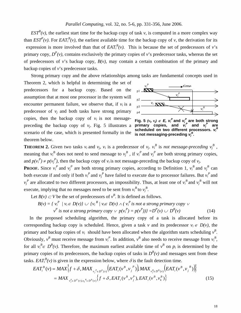
Strong primary copy and the above relationships among tasks are fundamental concepts used in Theorem 2, which is helpful in determining the set of predecessors for a backup copy. Based on the assumption that at most one processor in the system will encounter permanent failure, we observe that, if vi is a predecessor of vj and both tasks have strong primary copies, then the backup copy of vi is not message-preceding the backup copy of vj. Fig. 5 illustrates a scenario of the case, which is presented formally in the theorem below. THEOREM 2. Given two tasks vi and vj, vi is a predecessor of vj. vi
B is not message-preceding vjB ,
meaning that viB does not need to send message to vj
B , if viP and vj
P are both strong primary copies, and p(vi
P) ≠ p(vjP), then the backup copy of vi is not message-preceding the backup copy of vj.
PROOF. Since viP and vj
P are both strong primary copies, according to Definition 1, viB and vj
B can both execute if and only if both vi
P and vjP have failed to execute due to processor failures. But vi
P and vj
P are allocated to two different processors, an impossibility. Thus, at least one of viB and vj
B will not execute, implying that no messages need to be sent from vi
B to vjB. �
Let B(v) ⊂ V be the set of predecessors of vB. It is defined as follows. B(v) = { vi
P | vi ∈ D(v)} ∪ {vi B | vi∈ D(v) ∧ ( vi
P is not a strong primary copy ∨ vP is not a strong primary copy ∨ p(vi
P) = p(vP))} =DP(v) ∪ DB(v) (14) In the proposed scheduling algorithm, the primary copy of a task is allocated before its
corresponding backup copy is scheduled. Hence, given a task v and its predecessor vi ∈ D(v), the primary and backup copies of vi should have been allocated when the algorithm starts scheduling vB. Obviously, vB must receive message from vi
P. In addition, vB also needs to receive message from viB,
for all viB∈ DB(v). Therefore, the maximum earliest available time of vB on pi is determined by the
primary copies of its predecessors, the backup copies of tasks in DB(v) and messages sent from these tasks. EATi
B(v) is given in the expression below, where δ is the fault detection time.
( ) ( ){ }),(,),(,)( )()(B
jB
ivDvP
jB
ivDvB
i vvEATMAXvvEATMAXfMAXvEAT BBj
PPj ∈∈
+= δ
{ }),(),,(,)(),(
Bk
Bi
Pj
BivDvvDv
vvEATvvEATfMAX BBk
PPj
δ+=∈∈
(15)
p1
p4
p2
time
vjB
vi
vjP
viP
p3
Fig. 5 (vi, vj) ∈ E, viP and vj
P are both strongprimary copies, and vi
P and vjP are
scheduled on two different processors. viB
is not messaging-preceding vjB.
18

Parallel Computing, vol. 32, no. 5-6, pp. 331-356, June 2006.
ESTiB(v) and ESTB(v) denote the earliest start time for the backup copy of v on pi, and the earliest
start time for the backup copy of task v on any processor, respectively. The computation of ESTiB(v) is
more complex than that of ESTiP(v), due to the need to judiciously overlap some backup copies on
the same processor. The computation of ESTiB(v) can be found from step 3.2.4 in the above algorithm.
In the eFRD algorithm, the BOV scheme is implemented in step 3.2, which attempts to reduce schedule length by selectively overlapping backup copies of tasks. The expression for ESTB(v) is given below,
{ })()( )( vESTMINvEST BivFp
Bi∈
= (16)
Unlike expression (13) for ESTP(v), the candidate processor pi in (16) is not chosen directly from the set P. Instead, it is selected from F(v), a set of feasible processors to which the backup copy of v can be allocated. Obviously, p(vP) is not an element of F(v). Furthermore, given a task v, it is observed that under some special circumstances described below, vB cannot be scheduled on the processor where the primary copy of v's predecessor vi
P is scheduled (Fig. 6 illustrates this scenario). The set F(v) can be generated with help of Theorem 3. Theorem 3. Given two tasks vi and vj, (vi, vj)∈ E, if vi
B is not schedule-preceding vjP, then vj
B and viP
can not be allocated to the same processor. PROOF. Suppose p(vi
P) has failed before time fi, and viB executes instead of vi
P. Thus, either viB is
execution-preceding vjP or vi
B is execution-preceding vjB. But vi
B cannot be execution-preceding vjP,
since viB is not schedule-preceding vj
P. Hence, viB must be execution-preceding vj
B. This implies that vj
B executes on a processor, which is operational before fjB. Since a fault occurs on p(vi
P) before fjB,
vjB is not scheduled on p(vi
P), thus, p(vjB) ≠ p(vi
P). � Recall that EATi(v, vj) in expression (11) is a basic parameter used to derive EATi
P(v) in expression (12) and EATi
B(v) in expression (12). EATi(v, vj) is determined by the start time MSTik(e) of message e sent from pi = p(v) to pk = p(vj). MSTik(e) depends on how the message is routed and scheduled on the links. Thus, a message is allocated to a link if the link has an idle time slot that is later than the sender’s finish time and is large enough to accommodate the message. MSTik(e) is computed by the following procedure, where e = (vj, v), MST(er+1) = ∞, MST(e0) = 0, |e0| = 0, and
viB
vjB
p1
p2
timeviP
vjP
p3
Fig. 7 vi is the predecessor of vj, viP and vj
P arescheduled on the same processor, and vi
P isthe strong primary copy. In this case, vi
B is notexecution-preceding vj
P.
p1
p2
p3
time vjB
vjB
vjP vi
B
viP
Fig. 6 (vi, vj) ∈ E, viB,is not schedule-preceding
vjP and vi
P is a strong primary copy. vjB can
not be scheduled on the processor on whichvi
P is scheduled.
19

Parallel Computing, vol. 32, no. 5-6, pp. 331-356, June 2006.
MQi = {e1, e2, …, er} is the message queue containing all messages scheduled to the link from pi to pk. This procedure behaves in a similar manner as the previous procedure for computing the earliest start time of a task.
Computation of MSTik(e): 1. for (g = 0 to r + 1) do /* Check whether the idle time slots */ 2. if MSTik(eg+1) - MAX{MSTik(eg) + wik*|eg|, f(vj)} ≥ wik*|e| then /* If the idle time slots 3. return MSTik(eg) + wik*|eg|, f(vj); /* can accommodate v, return the value */ 4. end for5. return ∞; /* No such idle time slots is found, MST is set to be ∞ */
In scheduling messages, the proposed algorithm tries to avoid sending redundant messages in step 3.6, which is based on the following theorem. This scheme enhances the performance by consuming less communication resources. Suppose vj
P has successfully executed, either viP is execution-
preceding vjP or vi
B is execution-preceding vjP. We observe that, in a special case illustrated in Fig 7,
viB will never be execution-preceding vj
P. This statement is described and proved in Theorem 4. THEOREM 4. Given two tasks vi and vj, (vi, vj)∈ E, if the primary copies of vi and vj are allocated to the same processor and vi
P is a strong primary copy, then viB is not execution-preceding vj
P, meaning that sending a message from vi
B to vjP would be redundant.
PROOF. By contradiction: Assume viB is execution-preceding vj
P, thus, both viB and vj
P must execute (Def. 4). Since vi
P is a strong primary copy, processor p(viP) must have failed before time fi (Def. 1).
But viP and vj
P are allocated to the same processor and viP is schedule-preceding vj
P, implying that vjP
also could not execute. A contradiction. � Additionally, we identify another enlightening
principle, based on which redundant messages can be eliminated. Fig. 8 shows a scenario that there is no need for a message to be delivered from vi
P to vjB.
The rationale behind this case is proved in the following theorem. It is assumed that if p1 fails during the execution of vj
P, viB will have to be
executed to send a message to vjB.
THEOREM 5 Given two tasks vi and vj, (vi, vj)∈ E, if the primary copies of vi and vj are allocated to the same processor, vj
P is a strong primary copy, and vjP is schedule-preceding vi
B, then viP is not
message-preceding vjB, indicating that a message from vi
P to vjB is not required.
PROOF. Suppose vjB is executed. We know that processor p(vj
P) must have failed before fj due to the nature of strong primary copy of vj (Def. 1). Since vi
P is assigned to p(vjP), vi
P is unable to successfully execute if p(vj
P) has failed before fj, otherwise viP might have been completed. In this
case, viB takes an opportunity to start executing, because vi
B’s start time is later than the finish time of
viB
vjB
Fig. 8 vi is the predecessor of vj, viP and vj
P arescheduled on the same processor, vi
P is thestrong primary copy, vj
P is schedule-precedingvi
B. Hence, viB is not message-preceding vj
P.
p1
p2
viP vj
P time
p3
20
Parallel Computing, vol. 32, no. 5-6, pp. 331-356, June 2006.
viP and vj
P (vjP is schedule-preceding vi
B). Thus, it is guaranteed that vjB can receive a message from vi
B when p(vj
P) fails, making a message sent from viP to vj
B redundant. �
5 PERFORMANCE EVALUATION In this section, we compare the performance of the proposed algorithm with three existing real-
time fault-tolerant scheduling algorithms in the literature, namely, OV [21], FGLS [10][11], and FRCD[24] by extensive simulations. For the purpose of comparison, we also simulated a non fault-tolerant real-time scheduling algorithm (referred to as NFT hereafter) that is unable to tolerate any failure. In this study, we considered a real world application in addition to synthetic workloads.
Three performance measures are used to capture three important but different aspects of real-time and fault-tolerant scheduling. The first measure is schedulability (SC), defined to be the percentage of parallel real-time jobs that have been successfully scheduled among all submitted jobs, which measures an algorithm’s ability to find a feasible schedule. The second is reliability, defined in expression (2), which describes the reliability of a feasible schedule. Reflecting the combined performance of the first two measures, the third measure, performability (PF), is defined to be a product of schedulability and reliability. Formally,
SC = Number of jobs with feasible schedules /Total number of submitted jobs (17) PF(Λ, Μ, X, XB,T) = R(Λ, Μ, X,XB,T) × SC (18)
In the following discussions, performability serves as a single scalar metric that measures the overall performance of a real-time heterogeneous system.
Recall that while the four algorithms to be compared share some features such as being fault-tolerant and static, they differ in some other aspects such as task dependence and heterogeneity. OV assumes independent tasks and homogeneous systems, whereas FRCD, eFRD and FGLS consider tasks with precedence constraints that execute on heterogeneous systems. Since FGLS is developed for systems where the communication link is single bus, the communication heterogeneity is not considered in FGLS. Additionally, while FRCD and eFRD incorporate computational, communication and reliability heterogeneities into the scheduling, FGLS considers only computational heterogeneity. In order to make the comparison fair and meaningful, some adjustments have to be made to the algorithms. More specifically, when comparing all four algorithms in Sections 5.2 and 5.3, both FGLS, FRCD and eFRD are downgraded to handle only independent tasks that execute on homogeneous systems, by removing precedence constraints from tasks, making the underlying system homogeneous, and assuming fixed deadlines for all tasks.
Similarly, when comparisons are made between eFRD and FGLS in Sections 5.4 and 5.5, the eFRD algorithm is downgraded by assuming communication homogeneity, while the FGLS algorithm is adapted to include reliability heterogeneity. Furthermore, the FGLS algorithm does not explicitly show how deadlines are considered, implying that FGLS might be designed for soft real-time systems.
21

Parallel Computing, vol. 32, no. 5-6, pp. 331-356, June 2006.
Therefore, SC cannot be directly measured in FGLS. In order for the comparison to be meaningful, we made minor modifications to FGLS so that deadlines are explicitly considered in scheduling tasks, thereby making SC measurable.
5.1 Workload and System Parameters Workload parameters are chosen in such a way that they are either based on those used in the
literature or represent reasonably realistic workload and provide some stress tests for the algorithms. We studied three types of task graphs (DAGs): binary tree, lattice and DAGs with random precedence constraints, ones that have been frequently used by researchers in the past [23][27][28].
In each simulation experiment, 100,000 real-time DAGs were generated independently for the scheduling algorithm as follows: First, for each DAG, determine the number of real-time tasks N, the number of processors m and their failure rates R = {λ1, λ2, …, λm}. Then, the computation time in the execution time vector C is randomly chosen from a uniformly range EX = [5, 50]. The scale of this range approximates the level of computational heterogeneity. Data communication among real-time tasks and communication weights are randomly selected from uniformly ranges V =[1, 10]. Finally, the fault detection time δ is randomly computed according to a uniform distribution in the range between 1 and 10, because the fault detection time on average is approximately 3 ms [31]. Real-time deadlines can be defined in two ways: 1. A single deadline is associated with a real-time job, which is a set of tasks with or without
precedence constraints. Such a deadline is referred to as a common deadline in the literature [19][20]. Common deadlines were used in simulation studies reported in Sections 5.2 and 5.3.
2. Individual deadlines are associated with tasks within a real-time job. This deadline definition is often used for the dynamic scheduling of independent real-time tasks [9][16]. In simulation studies reported in Sections 5.4 and 5.5, this deadline definition was adapted for tasks of a real-time job with precedence constraints. More specifically, given vi ∈V, if vi is on pk and vj is on pl, then vi’s deadline is determined by: di = MAX{dj + eij×wlk} + MAX{cik} + t, (19) where t is a constant chosen uniformly from a given range H that represents individual relative deadlines.
A DAG with random precedence constraints is generated in four steps: First, the number of tasks N and the number of messages U are chosen. In this simulation study, it is assumed that U = 4N. Second, the execution time for each task is chosen randomly. Third, the communication time for each message is generated randomly and its sender and receiver selected randomly, subject to the condition that such selection does not generate any circle in the graph. Finally, a relative deadline t for each task is selected uniformly from a given H.
5.2 Schedulability This experiment evaluates performance in terms of schedulability among the five algorithms
using the schedulability measure. The workload consists of sets of independent real-time tasks
22

Parallel Computing, vol. 32, no. 5-6, pp. 331-356, June 2006.
23
0.5
0.6
0.7
0.8
0.9
3.5 4 4.5 5 5.5 6 6.5 7 7.5
OV eFRDFGLS FRCD
MAX_F(10 -6)
Reliability
running on a homogeneous system. The size of the task set is fixed at 100 tasks and the size of the homogeneous system is fixed at 20. A common deadline of 100 is selected. SC is first measured as a function of task execution time in the range between 19 and 29 with increments of 1 (see Fig. 9), and
then measured as a function of task set size (see Fig. 10). Figs. 9 and 10 show that the schedulabilities of the OV and eFRD algorithms are almost identical,
and so are the FGLS and FRCD algorithms. Considering that the eFRD algorithm has to be downgraded for comparability, this result should imply that eFRD is more powerful than OV, because eFRD can also schedule tasks with precedence constraints to be executed on heterogeneous systems, which OV is not capable of. The results indicate that high reliabilities are made possible by eFRD at the cost of schedulability, because the average SC value of NFT is approximately 7% higher than that of eFRD.
The results further reveal that both OV and eFRD significantly outperform FGLS and FRCD in SC, suggesting that both FGLS and FRCD are not suitable for scheduling independent tasks. The reason for FGLS’s poor performance can be explained by the fact that, like FRCD, it does not employ the overlapping scheme for backup copies. The consequence is twofold. First, FGLS and FRCD require more computing resources than eFRD, which is likely to lead to a relatively low SC when the number of processors is fixed. Second, unlike eFRD, the backup copies in FGLS and FRCD cannot overlap with one another on the same processor, and this may result in a much longer schedule length.
0
0.2
0.4
0.6
0.8
1
7 8 9 10 11 12 13
NFT OV eFRDFGLS FRCD
Number of task (x10)
Scheduability
0
0.2
0.4
0.6
0.8
1
19 20 21 22 23 24 25 26 27 28 29
NFT OV eFRDFGLS FRCD
Execution time
Schedulability
Fig. 10. Schedulability as a function of N. Common deadline = 100, m = 16, MIN_F = 0.5*10-6, MAX_F = 3.0*10-6, EX = [1, 20].
Fig. 9. Schedulability of independent tasks as a function of execution time. Common deadline = 100, N = 100, m = 20.
Fig. 11 Reliability as function of MAX_F. N = 50, m = 20, MIN_F = 1*10-6, EX = [500, 1500].
Parallel Computing, vol. 32, no. 5-6, pp. 331-356, June 2006.
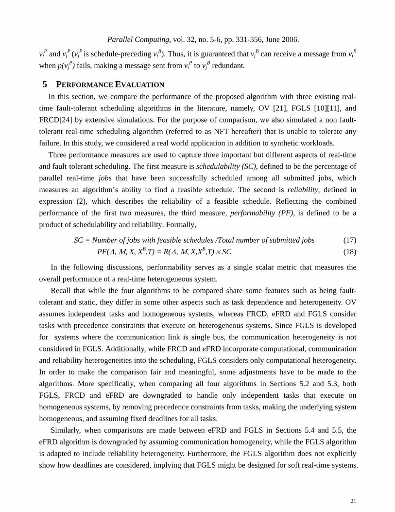
5.3 Reliability Performance In this experiment, the reliability of the OV, FGLS, FRCD and eFRD algorithms are evaluated as
a function of maximum processor failure rate, shown in Fig. 11. To stress the reliability performance, schedulabilities of all the four algorithms are assumed to be
1.0 by assigning extremely loose deadlines for tasks. The task set size and system sizes are 200 and 20, respectively. Execution time of each task is chosen uniformly from the range between 500 and 1500, and the failure rates were uniformly selected from the range between MIN_F and MAX_F. In this experiment, MIN_F is 1.0*10-6 per hour and MAX_F varies from 3.5*10-6 to 7.5*10-6 per hour with increments of 0.5*10-6. The link failure rates are taken uniformly in the range from 0.65×10⁻⁶ to 0.95×10⁻⁶ per hour.
We observed from Fig. 11 that the reliability of OV and FGLS are very close, and so are those of FRCD and eFRD. FRCD and eFRD perform considerably better than both OV and FGLS, with R values being approximately from 10.5% to 22.3% higher than those of OV and FGLS. The FRCD and eFRD algorithms have much better reliability simply because OV and FGLS do not consider reliability in their scheduling schemes while both FRCD and eFRD take reliability into account. This experimental result validates the use of FRCD and eFRD to enhance the reliability, especially when tasks either have loose deadlines or no deadlines (non-real-time systems).
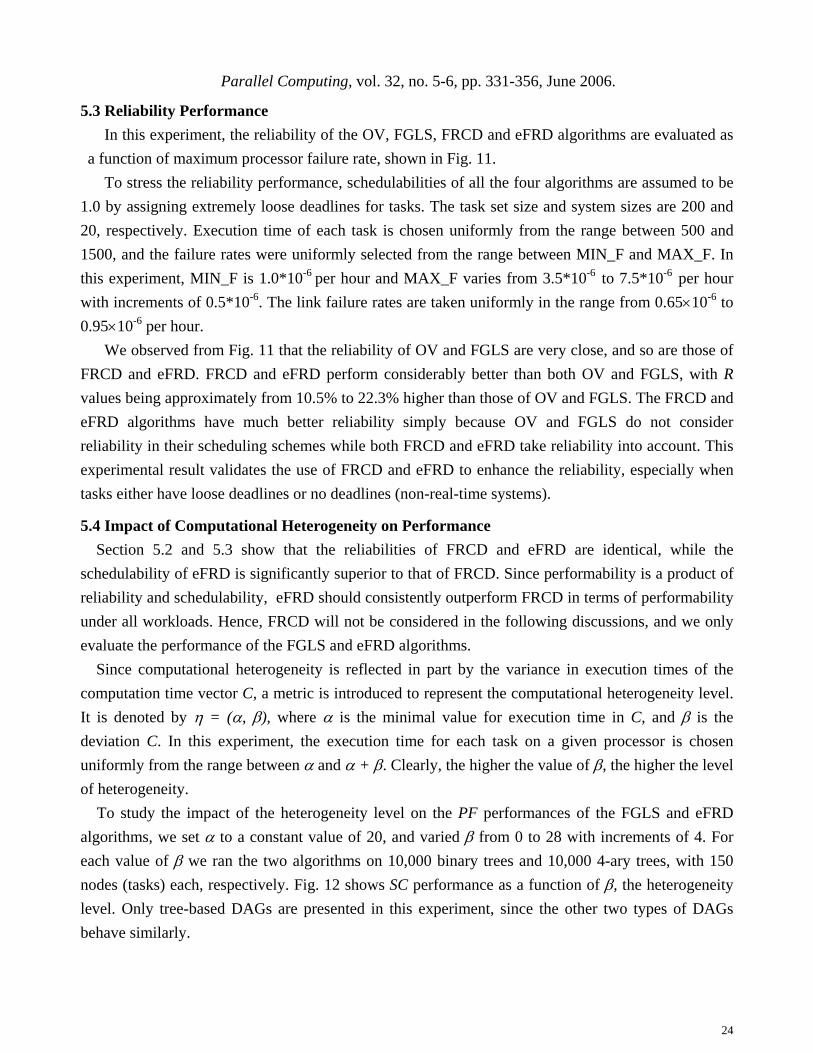
5.4 Impact of Computational Heterogeneity on Performance Section 5.2 and 5.3 show that the reliabilities of FRCD and eFRD are identical, while the
schedulability of eFRD is significantly superior to that of FRCD. Since performability is a product of reliability and schedulability, eFRD should consistently outperform FRCD in terms of performability under all workloads. Hence, FRCD will not be considered in the following discussions, and we only evaluate the performance of the FGLS and eFRD algorithms.
Since computational heterogeneity is reflected in part by the variance in execution times of the computation time vector C, a metric is introduced to represent the computational heterogeneity level. It is denoted by η = (α, β), where α is the minimal value for execution time in C, and β is the deviation C. In this experiment, the execution time for each task on a given processor is chosen uniformly from the range between α and α + β. Clearly, the higher the value of β, the higher the level of heterogeneity.
To study the impact of the heterogeneity level on the PF performances of the FGLS and eFRD algorithms, we set α to a constant value of 20, and varied β from 0 to 28 with increments of 4. For each value of β we ran the two algorithms on 10,000 binary trees and 10,000 4-ary trees, with 150 nodes (tasks) each, respectively. Fig. 12 shows SC performance as a function of β, the heterogeneity level. Only tree-based DAGs are presented in this experiment, since the other two types of DAGs behave similarly.
24

Parallel Computing, vol. 32, no. 5-6, pp. 331-356, June 2006.
The first observation from Fig. 12 is that the value of PF increases with the heterogeneity level. This is because PF is a product of SC and R, and both SC and R become higher when the heterogeneity level increases. These results can be further explained by the following reasons. First,
though the individual relative deadlines (i.e. t in expression (19)) are not affected by the change in computational heterogeneity, high variance in task execution times does affect the absolute deadlines (i.e. d(vi) in expression (19)), making the deadlines looser and the SC higher. Second, high variance in task execution times also provides opportunities for more tasks to be packed in with the fixed number of processors, giving rise to a higher SC. Third, RC decreases as the heterogeneity level increases, implying an increasing R. This is because high variance in execution times will lead to a low minimum execution time in C. Given the greedy nature of both algorithms, processors with minimum execution time in C are most likely to be chosen for task execution, giving rise to high reliability as a function of processor execution time and processor failure rates.
The second interesting observation is that eFRD outperforms FGLS with respect to PF at low
heterogeneity levels while the opposite is true for high heterogeneity levels. This is because when heterogeneity levels are low, both SC and R of eFRD are considerably higher than those of FGLS (Reliabilites are depicted in Fig. 13). On the other hand, eFRD’s SC is lower than that of FGLS at a high heterogeneity level, and Rs of two algorithms becomes similar (eFRD is slightly better than FGLS) when heterogeneity level increases. Therefore, eFRD’s PF, the product of SC and R, is lower than that of FGLS at high heterogeneity levels.
This result suggests that, if schedulability is the only objective in scheduling, FGLS is more suitable for systems with relatively high levels of heterogeneity, whereas eFRD is more suitable for scheduling tasks with relatively low levels of heterogeneity. In contrast, if R is the sole objective, eFRD is consistently better than FGLS.
0
0.15
0.3
0.45
0.6
0.75
0 4 8 12 16 20 24 28
FGLS(btree) eFRD(btree)FGLS(4-ary tree) eFRCD(4-ary tree)
Beta
Reliability
00.10.20.30.40.50.60.70.8
0 4 8 12 16 20 24 28
FGLS(btree) eFRCD(btree)FGLS(4-ary tree) eFRCD(4-ary tree)
Beta
Performability
Fig. 13 Reliability of btrees and 4-ary treesas a function of heterogeneity level. H = [1,100], N = 150, m=20, alpha = 20
Fig. 12 Performability of btrees and 4-ary trees as a function of heterogeneity level. H = [1, 100], N = 150, m=20, alpha = 20
25

Parallel Computing, vol. 32, no. 5-6, pp. 331-356, June 2006.
In addition, Fig. 12 indicates that performability of FGLS increases much more rapidly with heterogeneity level than that of eFRD, implying that FGLS is more sensitive to the change in computational heterogeneity than eFRD. This is because both SC and R (See Fig.13) of FGLS
continuously increase more sharply with the increasing heterogeneity level than those of eFRD. Fig. 13 depicts the R as a function of computational heterogeneity level. The simulation parameters
are the same as the above experiment. Fig. 13 reveals that R increases as the heterogeneity level increases. This is because high variance in execution times will lead to a low minimum execution time in C. Given the greedy nature of both algorithms, processors with minimum execution time in C are most likely to be chosen for task execution, giving rise to high reliability as R is a function of processor execution time and processor failure rate. Fig.13 shows that R of eFRD is consistently higher than that of FGLS, suggesting that eFRD is superior to FGLS in terms of reliability.
5.5 Impact of Task Parallelism on Schedulability One interesting observation from the previous experiments (Figures 12 and 13) is that task
parallelism, implied by the width of the tree in the DAGs (binary vs. 4-ary trees), has a significant impact on the SC performance while the R performance is insensitive to such task parallelism. In this section we present simulation results that substantiate this observation and establish the relationship between task parallelism and SC performance.
Fig. 14 shows an indirect relationship between SC and task parallelism of random task graphs
containing a fix number of tasks, by plotting SC as a function of the number of messages in the task graph. For a task graph with a fixed number of tasks, the more messages there are among tasks, the more precedence constraints that are imposed on the tasks, implying that fewer tasks may execute concurrently. In other words, task parallelism decreases as the number of messages increases.
Fig. 14 plainly shows that the schedulabilities of FGLS and eFRD are very close when the number of messages is greater than 260, with FGLS outperforming eFRD slightly. As the number of messages
0
0.2
0.4
0.6
0.8
320 260 280 260 240 220 200 180 160 140
1 FGLSeFRD
Number of messages
Schedulability
0
0.2
0.4
0.6
0.8
1
2 3 4 5 6 7 8 9
FGLS
eFRCD
Degrees
Schedulability
Fig. 15. Schedulability of trees as a function ofthe number of branches. H = [1, 100], N = 200,m = 10, EX = [1, 20], COM = [1, 10].
Fig. 14. Schedulability of random graphs as afunction of the number of messages. H = [1, 10], N= 100, m = 16, EX = [1, 20], COM = [1, 10].
26
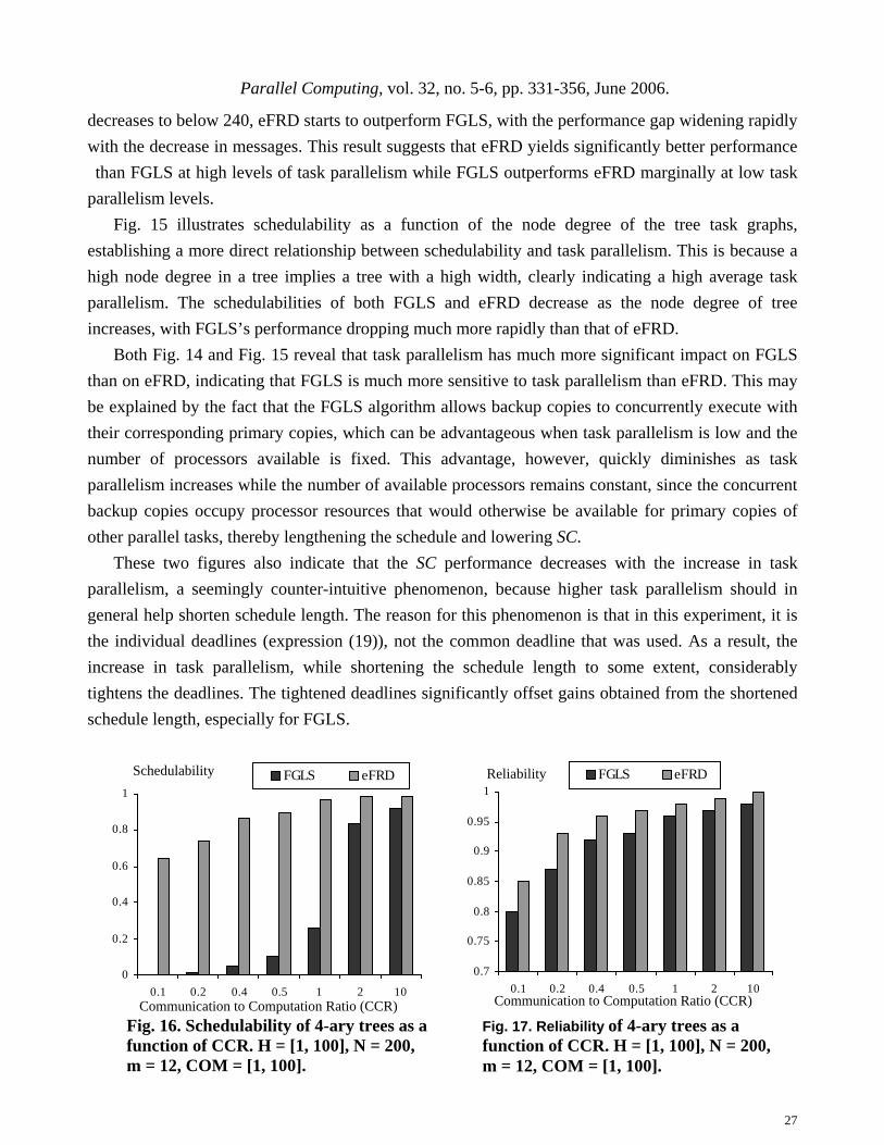
Parallel Computing, vol. 32, no. 5-6, pp. 331-356, June 2006.
decreases to below 240, eFRD starts to outperform FGLS, with the performance gap widening rapidly with the decrease in messages. This result suggests that eFRD yields significantly better performance than FGLS at high levels of task parallelism while FGLS outperforms eFRD marginally at low task
parallelism levels. Fig. 15 illustrates schedulability as a function of the node degree of the tree task graphs,
establishing a more direct relationship between schedulability and task parallelism. This is because a high node degree in a tree implies a tree with a high width, clearly indicating a high average task parallelism. The schedulabilities of both FGLS and eFRD decrease as the node degree of tree increases, with FGLS’s performance dropping much more rapidly than that of eFRD.
Both Fig. 14 and Fig. 15 reveal that task parallelism has much more significant impact on FGLS than on eFRD, indicating that FGLS is much more sensitive to task parallelism than eFRD. This may be explained by the fact that the FGLS algorithm allows backup copies to concurrently execute with their corresponding primary copies, which can be advantageous when task parallelism is low and the number of processors available is fixed. This advantage, however, quickly diminishes as task parallelism increases while the number of available processors remains constant, since the concurrent backup copies occupy processor resources that would otherwise be available for primary copies of other parallel tasks, thereby lengthening the schedule and lowering SC.
These two figures also indicate that the SC performance decreases with the increase in task parallelism, a seemingly counter-intuitive phenomenon, because higher task parallelism should in general help shorten schedule length. The reason for this phenomenon is that in this experiment, it is the individual deadlines (expression (19)), not the common deadline that was used. As a result, the increase in task parallelism, while shortening the schedule length to some extent, considerably tightens the deadlines. The tightened deadlines significantly offset gains obtained from the shortened schedule length, especially for FGLS.
27
0
0.2
0.4
0.6
0.8
1
0.1 0.2 0.4 0.5 1 2 10
FGLS eFRD
Communication to Computation Ratio (CCR)
Schedulability
0.7
0.75
0.8
0.85
0.9
0.95
1
0.1 0.2 0.4 0.5 1 2 10
FGLS eFRD
Communication to Computation Ratio (CCR)
Reliability
Fig. 17. Reliability of 4-ary trees as a function of CCR. H = [1, 100], N = 200, m = 12, COM = [1, 100].
Fig. 16. Schedulability of 4-ary trees as a function of CCR. H = [1, 100], N = 200, m = 12, COM = [1, 100].

Parallel Computing, vol. 32, no. 5-6, pp. 331-356, June 2006.
5.6 Impact of Communication to Computation Ratio on Performance In this section we evaluate the impact of communication to computation ratio (CCR), which
indicates the ratio of the average execution time of communication activities to that of computation activities. A large value of CCR means a relatively high communication load compared with computation load. In this experiment we varied CCR within [0.1, 10]. First, the communication cost of each message is randomly chosen from a uniform distribution. Next, the execution cost of each task is randomly generated according to the given CCR value.
Fig. 16 reveals that when the CCR value is small (less than or equal to 1), the schedulability of eFRD is significantly higher than that of FGLS. The SC performance improvement of eFRD over FGLS decreases as the CCR value increases. This result implies that eFRD performs substantially better than FGLS with small values of CCR while FGLS. outperforms eFRD marginally at low task parallelism levels.
Fig. 17 clearly shows that CCR has noticeable impacts on both FGLS and eFRD. It is observed from Fig. 17 that the reliabilities yielded by FGLS and eFRD increase with the increasing values of CCR, indicating that a large CCR value leads to high reliabilities. These results can be explained by the way of choosing execution times. Specifically, larger CCR values result in smaller execution times of tasks, which in turn induce higher reliabilities. Similar to the schedulability performance, the reliability improvement of eFRD over FGLS is pronounced when the CCR value is small. However, this advantage gradually diminishes as the CCR value goes up. This is mainly because execution times become a whole lot shorter with large CCR values. The shortened execution times cause relatively higher reliabilities, leaving limited room for further improvement in reliability.
5.7 Performance on a Real Application
The goal of this experiment is three-fold: First, to validate the results from the synthetic
application cases; second, to evaluate the impact of processor numbers on the performance of the
proposed algorithm; and third, to test the scalability of our algorithm. To do so, we evaluate the
performance of eFRD with very large task graphs generated from a real application: a digital signal
processing (DSP) system with 119 tasks in the task graph [30]. Since OV assumes independent tasks
and homogeneous systems, we only compare eFRD against FRCD and FGLS, which can handle tasks
with precedence constraints executing on heterogeneous systems.
The number of processors of a simulated heterogeneous system is varied from 9 to 16. The failure
rates of the processors, which are fully connected with one another, are chosen randomly between
1×10⁻⁶ and 7.5×10⁻⁶. Similarly, the link failure rates of the system are uniformly in the range from
28

Parallel Computing, vol. 32, no. 5-6, pp. 331-356, June 2006.
0.65×10⁻⁶ to 0.95×10⁻⁶ per hour [28]. We performed the experiment with ranges for generating
deadlines set to 500ms. From Fig. 18, it can be seen that the increase in number of processors
increases the schedulability for all the three algorithms. Importantly, eFRD improves the
performance in schedulability over FGLS and FRCD by up to 1823% and 127% (with average of
374% and 64%), respectively. Furthermore, the advantage of eFRD over FGLS and FRCD becomes
more pronounced when the number of processors is small, and the performance improvement in
schedulability decreases as the number of processors increases. This is because when the number of
processors is large, there is less likelihood that the processors are the bottleneck of in performance.
The results indicate that the proposed algorithm can substantially improve system schedulability over
the existing algorithms under circumstances where processors are critical resources in heterogeneous
systems.
The reliabilities of the three alternatives are presented in Fig. 19. We find that the eFRD algorithm
improves the reliability of FGLS by more than 15.7% while maintaining the same level of reliability
as that of FRCD. This is because eFRD leverages the reliability-cost driven technique to achieve the
high reliability. From Figures 18 and 19 we conclude that the proposed algorithm can provide reliable
allocations for both small- and large-scale applications while significantly improving resource
utilization.
6. CONCLUSION In this paper we propose an efficient fault-tolerant scheduling algorithm (eFRD), in which real-
time tasks with precedence constraints can tolerate one processor’s failures in a heterogeneous system
with fully connected network. The fault-tolerant capability is incorporated in the algorithm by using a
0
0.2
0.4
0.6
0.8
1
9 10 11 12 13 14 15 16
FGLS FRCD eFRD
Number of Processors
Schedulability
0
0.2
0.4
0.6
0.8
1
9 10 11 12 13 14 15 16
eFRD FGLS FRCD
Number of Processors
Reliability
Fig. 19. Reliability results for a real world application: a digital signal processing system.
Fig. 18. Schedulability results for a real world application: a digital signal processing system.
29

Parallel Computing, vol. 32, no. 5-6, pp. 331-356, June 2006.
Primary/Backup (PB) model, where failures are detected after a fixed amount of time. In this PB
model, each task is associated with a primary copy and a backup copy that are allocated to two
different processors and the backup copy is executed only if the primary copy fails due to the
permanent failure of one processor. Unlike FRCD [24], the eFRD algorithm relaxes the requirement
in FRCD that forbids the overlapping of any backup copies to allow such overlapping on the same
processor if their corresponding primary copies are allocated to different processors. The system
reliability is further enhanced by assigning tasks to processors that are able to yield high reliability.
Moreover, the algorithm takes system and workload heterogeneity into consideration by explicitly
accounting for computational, communication, and reliability heterogeneity.
To the best of our knowledge, the proposed algorithm is the first of its kind reported in the
literature, in that it most comprehensively addresses the issues of fault-tolerance, reliability, real-time,
task precedence constraints, and heterogeneity. To assess the performance of eFRD, extensive
simulation studies were conducted to quantitatively compare it with the three most relevant existing
scheduling algorithms in the literature, OV [21], FGLS [10][11], and FRCD [24]. The simulation
results indicate that the eFRD algorithm is considerably superior to the three algorithms in the vast
majority of cases. There are two exceptions, however. First, the FGLS outperforms eFRD marginally
when task parallelism is low. Second, when computational heterogeneity is high, the eFRD algorithm
becomes inferior to the FGLS algorithm.
The experimental results also indicate that both computational heterogeneity and task parallelism
have a significant impact on the schedulability. In particular, the FGLS algorithm is much more
sensitive to computational heterogeneity and task parallelism than the eFRD algorithm.
Acknowledgments This is a substantially revised and improved version of a preliminary paper [23] appeared in the Proceeding of the International Conference on Parallel Processing (ICPP2002), pages 360-368, August 2002. The revisions include a detailed reliability analysis, an improved overlapping scheme, consideration of more workload and system parameters, and performance evaluation with a real application. This work was partially supported by NSF under Grant EPS-0091900, New Mexico Institute of Mining and Technology under Grant 103295, Intel Corporation under Grant 2005-04-070, and University of Nebraska-Lincoln under Grant 26-0511-0019.
REFERENCES [1] T.F. Abdelzaher and K.G. Shin., “Combined Task and Message Scheduling in Real-Time Systems,” IEEE
Trans. on Parallel and Systems, Vol. 10, No. 11, Nov. 1999. [2] K. Ahn, J. Kim, S. Hong, “Fault-Tolerant Real-Time Scheduling using Passive Replicas,” Proc. Pacific
Rim Int’l Symposium on Fault-Tolerant Systems, December 15-16, 1997.
30

Parallel Computing, vol. 32, no. 5-6, pp. 331-356, June 2006.
[3] R. Al-Omari, A.K. Somani, and G. Manimaran, “A new fault-tolerant technique for improving the schedulability in multiprocessor real-time systems,” Proc. Int’l Parallel and Processing Symposium, San
Francisco, USA, Apr. 2001. [4] N.M. Amato, P. An, “Task Scheduling and Parallel Mesh-Sweeps in Transport Computations,” Technical
Report TR00-009, Department of Computer Science, Texas A&M University, January 2000. [5] A. A. Bertossi, L. V. Mancini, F. Rossini, “Fault-Tolerant Rate-Monotonic First-Fit Scheduling in Hard-
Real-Time Systems,” IEEE Trans. Parallel and Systems, 10(9), pp. 934-945, 1999. [6] M. Caccamo and G. Buttazzo, “Optimal Scheduling for Fault-Tolerant and Firm Real-Time Systems,”
Proc. Int’l Conf. on Real-Time Computing Systems and Applications, Hiroshima, Japan, Oct. 27-29, 1998. [7] C. Dima, A. Girault, C. Lavarenne, and Y. Sorel, “Off-Line Real-Time Fault-Tolerant Scheduling,” Proc.
Euromicro Workshop on Parallel and Processing, pp. 410-417, Mantova, Italy, Feb. 2001. [8] A. Dogan, F. Ozguner, “Reliable matching and scheduling of precedence-constrained tasks in
heterogeneous computing,” Proc. Int’l Conf. on Parallel Processing, pp. 307-314, 2000. [9] S. Ghosh, R. Melhem and D. Mosse, “Fault-Tolerance through Scheduling of Aperiodic Tasks in Hard
Real-Time Multiprocessor Systems”, IEEE Trans. on Parallel and System, Vol 8, No 3, pp. 272-284, 1997 [10] A. Girault, C. Lavarenne, M. Sighireanu and Y. Sorel, “Fault-Tolerant Static Scheduling for Real-Time
Embedded Systems,” Proc. Int’l Conf. Computing Systems, April 2001. [11] A. Girault, C. Lavarenne, M. Sighireanu, and Y. Sorel, “Generation of Fault-Tolerant Static Scheduling
for Real-Time Embedded Systems with Multi-Point Links”, IEEE Workshop on Fault-Tolerant Parallel and Systems, San Francisco, USA, April 2001.
[12] C.J. Hou and K.G. Shin, “Allocation of Periodic Task Modules with Precedence and Deadline Constraints in Real-Time Systems”, IEEE Trans. on Computers, Vol.46, No.12, pp. 1338-1356, 1997.
[13] E.N. Huh, L.R. Welch, B.A. Shirazi and C.D. Cavanaugh, “Heterogeneous Resource Management for Dynamic Real-Time Systems,” Proc. the 9th Heterogeneous Computing Workshop, 287-296, 2000.
[14] Y.K. Kwok and I. Ahmad, “Static scheduling algorithms for allocating directed task graphs to multiprocessors,” ACM Computing Surveys, Vol.31 , No. 4, 1999, pp.406-471.
[15] F. Liberato, S. Lauzac, R. Melhem and D. Mosse, “Fault Tolerant Real-Time Global Scheduling on Multiprocessors,” Proc. of Euromicro Workshop in Real-Time Systems, 1999.
[16] F. Liberato, R. Melhem, and D. Mossé, “Tolerance to Multiple Transient Faults for Aperiodic Tasks in Hard Real-Time Systems,” IEEE Transactions on Computers, Vol. 49, No. 9, September 2000.
[17] G. Manimaran and C. Siva Ram Murthy, “A Fault-Tolerant Dynamic Scheduling Algorithm for Multiprocessor Real-Time Systems and Its Analysis,” IEEE Trans. on Parallel and Systems, Vol.9, No.11, November 1998.
[18] P. Mejia Alvarez and D. Mosse, “A Responsiveness Approach for Scheduling Fault Recovery in Real-Time Systems,” Proc. IEEE Real-Time Technology and Applications Symp., Canada, pp.1-10, June 1999.
[19] M. Naedele, “Fault-Tolerant Real-Time Scheduling under Execution Time Constraints,” Proc. Int’l Conf. on Real-Time Computing Systems and Applications, Hong Kong, China, Dec. 13 - 15, 1999.
[20] Y.Oh and S.H.Son, “An algorithm for real-time fault-tolerant scheduling in multiprocessor systems,” Proc. Euromicro Workshop on Real-Time Systems, Greece, 1992, pp.190-195.
[21]Y. Oh and S. H. Son, “Scheduling Real-Time Tasks for Dependability,” Journal of Operational Research Society, vol. 48, no. 6, pp 629-639, June 1997.
[22] X. Qin, and H. Jiang, “Dynamic, Reliability-driven Scheduling of Parallel Real-time Jobs in Heterogeneous Systems,” Proc. Int’l Conf. on Parallel Processing, Valencia, Spain, pp.113-122, 2001.
31

Parallel Computing, vol. 32, no. 5-6, pp. 331-356, June 2006.
[23] X. Qin, H. Jiang, D. R. Swanson, "An Efficient Fault-tolerant Scheduling Algorithm for Real-time Tasks with Precedence Constraints in Heterogeneous Systems," Proc. Int’l Conf. on Parallel Processing, British
Columbia, Canada, pp.360-368, Aug. 2002. [24] X. Qin, H. Jiang, and D. R. Swanson, “A Fault-tolerant Real-time Scheduling Algorithm for Precedence-
Constrained Tasks in Heterogeneous Systems,” Technical Report TR-UNL-CSE 2001-1003, Department of Computer Science and Engineering, University of Nebraska-Lincoln, September 2001.
[25] S. Ranaweera, and D.P. Agrawal, “Scheduling of Periodic Time Critical Applications for Pipelined Execution on Heterogeneous Systems,” Proc. Int’l Conf. on Parallel Processing, pp. 131-138, Sept. 2001.
[26] R.M. Santos, J. Santos, and J. Orozco, “Scheduling heterogeneous multimedia servers: different QoS for hard, soft and non real-time clients,” Proc. Euromicro Conf. on Real-Time Systems, pp.247-253, 2000.
[27]S.M. Shatz, J.P. Wang, and M. Goto, “Task Allocation for Maximizing Reliability of Computer Systems,” IEEE Trans. Computers, Vol.41, No.9, pp.1156-1168, Sept. 1992.
[28] S. Srinivasan, and N.K. Jha, “Safty and Reliability Driven Task Allocation in Systems,” IEEE Trans. Parallel and Systems, Vol.10, No.3, pp. 238-251, 1999.
[29] J. Stankovic, M. Spuri, K. Ramamritham and G.C. Buttazzo, “Deadline Scheduling for Real-time systems: EDF and Related Algorithms,” Kluwer Academic Publishers, 1998.
[30] C.M. Woodside and G.G. Monforton, “Fast Allocation of Processes in and Parallel Systems,” IEEE Trans. Parallel and Systems, Vol.4, No.2, pp.164-174, Feb. 1993.
[31] W. Zhao, L.E. Moser, and P.M. Melliar-Smith, “Unification of transactions and replication in three-tier architectures based on CORBA,” IEEE Trans. Dependable and Secure Computing, Vol. 2, No.1, pp.20 – 33, 2005.
[32] G. Buonanno, M. Pugassi, MG Sami, P. di Milano, “A High-Level Synthesis Approach to Design of Fault-Tolerant Systems,” Proc. IEEE VLSI Test Symposium, 1997.
[33] S. Hariri, A. Choudhary, and B. Sarikaya, “Architectural support for designing fault-tolerant open systems,” Computer, Vol. 25, No. 6, pp. 50 – 62, June 1992.
[34] T. D. Braun et al., “A comparison study of static mapping heuristics for a class of meta-tasks on heterogeneous computing systems,” Proc. Workshop on Heterogeneous Computing, pp.15-29, Apr. 1999.
[35] N.J. Boden, D. Cohen, and W.K. Su., “Myrinet: A Gigabit-per-second Local Area Network,” IEEE Micro, Vo. 15, No. 1, February 1995.
[36] J. Wu, P. Wyckoff, and D. K. Panda, “High Performance Implementation of MPI Datatype Communication over InfiniBand,” Proc. Int'l Parallel and Distributed Processing Symposium, April, 2004.
[37] K. Ramamritham, “Allocation and Scheduling of Precedence-Related Periodic Tasks,” IEEE Trans. Parallel and Distributed Systems, Vol. 6, No. 4, pp.412-420, 1995.
[38] G. Fohler, “Adaptive Fault-Tolerance with Statically Scheduled Real-Time Systems,” Proc. Euromicro Workshop on Real-Time Systems, June 1997.
[39] A. Dogan and F. Özgüner, “Matching and Scheduling Algorithms for Minimizing Execution Time and Failure Probability of Applications in Heterogeneous Computing,” IEEE Trans. Parallel and Distributed Systems, Vol. 13, No. 3, pp.308-323, 2002.
[40] A. Girault and H. Kalla and M. Sighireanu and Y. Sorel, “An Algorithm for Automatically Obtaining Distributed and Fault-Tolerant Static Schedules,” Proc. Int’l Conf. Dependable Systems and Networks, June 2003.
[41] I. Assayad and A. Girault and H. Kalla, “A Bi-Criteria Scheduling Heuristics for Distributed Embedded Systems Under Reliability and Real-Time Constraints,” Proc. Int’l Conf. Dependable Systems and Networks, June 2004.
32