a novel integrated modelling approach to design cost
TRANSCRIPT
A Novel Integrated Modelling Approach to Design Cost-effective Agri-Environment Schemes to Prevent Water Pollution and Soil Erosion from Cropland
— A Case Study of Baishahe Watershed in Shanxi Province, China
Zhengzheng Hao
Coauthors: Dr. Astrid Sturm, Prof. Frank Wätzold
Chair of Environmental Economics
2
Outline
Introduction
Study region
Methodology
Results
Discussion
Conclusion
Chair of Environmental Economics

3
Introduction — background and motivation
Intensive agricultural system has resulted in severe environmental risks,including soil erosion and water pollution in many regions (Evans et al., 2019)
A key policy instrument are agri-environment schemes (AES), payments tofarmers to address environmental problems, have been widely applied indeveloped countries (Wunder & Wertz, 2009)
Problems of AES include huge expense without adequate planning and designfor cost-effective measures, like Sloping Land Conversion Programme in China(Li & Liu, 2010)
To contribute the gap, a novel integrated modeling procedure can be apromising way to improve both:• Effectiveness of AES, with the intended environmental goals (reducing soil
erosion and water pollution) being actually achieved• Cost-effectiveness of AES, with maximized environmental goals under certain
budget, or minimized budget for given goals (Wätzold et al., 2016)
Chair of Environmental Economics
4
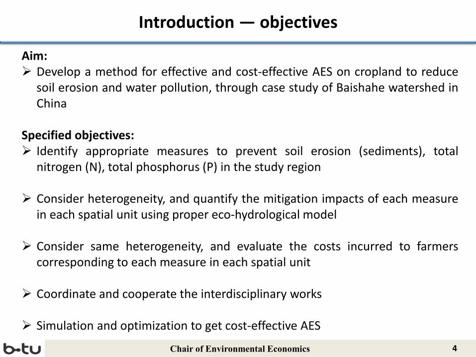
Introduction — objectives
Aim: Develop a method for effective and cost-effective AES on cropland to reduce
soil erosion and water pollution, through case study of Baishahe watershed inChina
Specified objectives: Identify appropriate measures to prevent soil erosion (sediments), total
nitrogen (N), total phosphorus (P) in the study region
Consider heterogeneity, and quantify the mitigation impacts of each measurein each spatial unit using proper eco-hydrological model
Consider same heterogeneity, and evaluate the costs incurred to farmerscorresponding to each measure in each spatial unit
Coordinate and cooperate the interdisciplinary works
Simulation and optimization to get cost-effective AES
Chair of Environmental Economics

5
(Source: Own results with ArcGIS, with data source of RESDC, 2015.)
Study region
Chair of Environmental Economics
Baishahe watershed
Area: 56 km2
Going through: Eight villagesMain activities: Small holder crop-livestock systemsLand-cover: Woodland, grassland, arable landMain crops: Winter wheat, corn
(Source: Material from Water Conservancy Bureau and Environment Protection Agency in Xia county.)

6
Methodology — framework
1. Cropland management measures
2. Input data collection
4. Agri-economic cost assessment
3. Mitigation impact assessment(SWAT model)
5. Simulation and optimization
6. Output: Mitigation impact and cost-effectiveness analysis
(Source: Modified based on Wätzold et al., 2016.)
Design AES: contract of five years (2018~2022), considering spatial heterogeneity

7(Source: USDA-NRCS, n.d., and materials from the Agricultural Bureau in Xia county.)
type measures code
structural measures
vegetative filter strip: 5 meters M1
vegetative filter strip: 10 meters M2
vegetative filter strip: 15 meters M3
tillage activities no-till M4
nutrient management
chemical fertilizer: 25% ↓ M5
chemical fertilizer: 40% ↓ M6
chemical fertilizer: 50% ↓ +swine manure 1000kg/ha
M7
chemical fertilizer: 50% ↓ +sheep manure 1000kg/ha
M8
crop planting cover crop: Soybean M9
cover crop: Corn M10
compounded chemical fertilizer: 25% ↓ + no till M11
chemical fertilizer: 40% ↓ + no till M12
Measure identification — selected measures

8
SWAT: Soil and Water Assessment Tool
Mitigation impact simulation — SWAT model
Channel/Flood PlainProcesses
Upland Processes
Channel/Flood PlainProcesses
(Source: Modified based on a presentation of Jeff Arnold.)
9
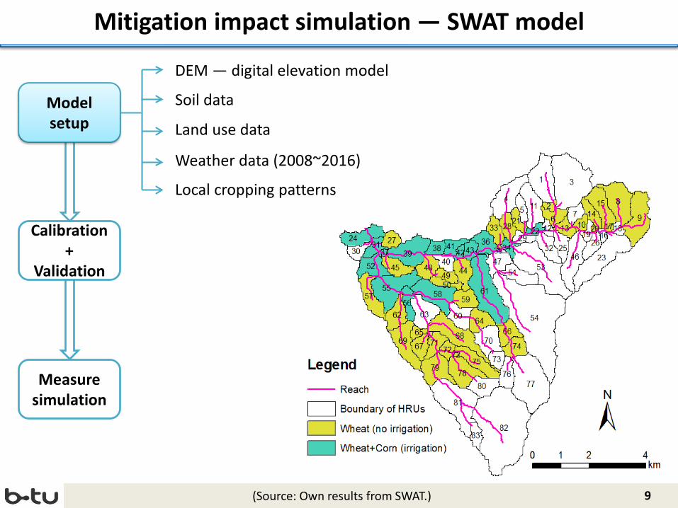
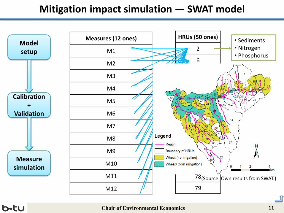
Mitigation impact simulation — SWAT model
Model setup
Calibration +
Validation
Measure simulation
Model setup
DEM — digital elevation model
Soil data
(Source: Own results from SWAT.)
Weather data (2008~2016)
Local cropping patterns
Land use data

10
Mitigation impact simulation — SWAT model
Model setup
Calibration +
Validation
Measure simulation
Model setup
Calibration +
Validation
Streamflow
Sediments
Nitrogen
Phosphorus
Crop yield
Chair of Environmental Economics
11
Mitigation impact simulation — SWAT model
Model setup
Calibration +
Validation
Measure simulation
Model setup
Calibration +
Validation
Measure simulation
Measures (12 ones)
M1
M2
M3
M4
M5
M6
M7
M8
M9
M10
M11
M12
HRUs (50 ones)
2
6
8
9
10…
……
……
……
.
78
79
• Sediments• Nitrogen• Phosphorus
Chair of Environmental Economics
(Source: Own results from SWAT.)

12
Cost assessment — cost categories
Measures
Structural measures:
M1, M2, M3
Non-structural measures:
M4, M5, M6, M7, M8, M9,
M10, M11, M12
Establishment costs
Maintenance costs
Foregone profits
Production costs
(Source: Based on Mettepenningen et al., 2017.)
𝑐𝑐𝑒𝑒𝑚𝑚
𝑐𝑐𝑚𝑚𝑚𝑚
𝑐𝑐𝑓𝑓𝑓𝑓
13
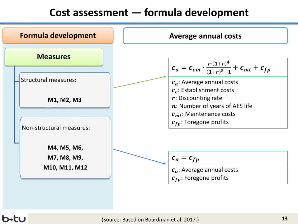
Cost assessment — formula development
Formula development Average annual costs
𝒄𝒄𝒂𝒂 = 𝒄𝒄𝒆𝒆𝒆𝒆 � 𝒓𝒓� 𝟏𝟏+𝒓𝒓𝟒𝟒
𝟏𝟏+𝒓𝒓 𝟓𝟓−𝟏𝟏+ 𝒄𝒄𝒆𝒆𝒎𝒎 + 𝒄𝒄𝒇𝒇𝒇𝒇
𝒄𝒄𝒂𝒂: Average annual costs𝒄𝒄𝒆𝒆: Establishment costs𝒓𝒓: Discounting rate𝒏𝒏: Number of years of AES life 𝒄𝒄𝒆𝒆𝒎𝒎: Maintenance costs 𝒄𝒄𝒇𝒇𝒇𝒇: Foregone profits
𝒄𝒄𝒂𝒂 = 𝒄𝒄𝒇𝒇𝒇𝒇𝒄𝒄𝒂𝒂: Average annual costs𝒄𝒄𝒇𝒇𝒇𝒇: Foregone profits
Measures
Structural measures:
M1, M2, M3
Non-structural measures:
M4, M5, M6, M7, M8, M9,
M10, M11, M12
(Source: Based on Boardman et al. 2017.)
14
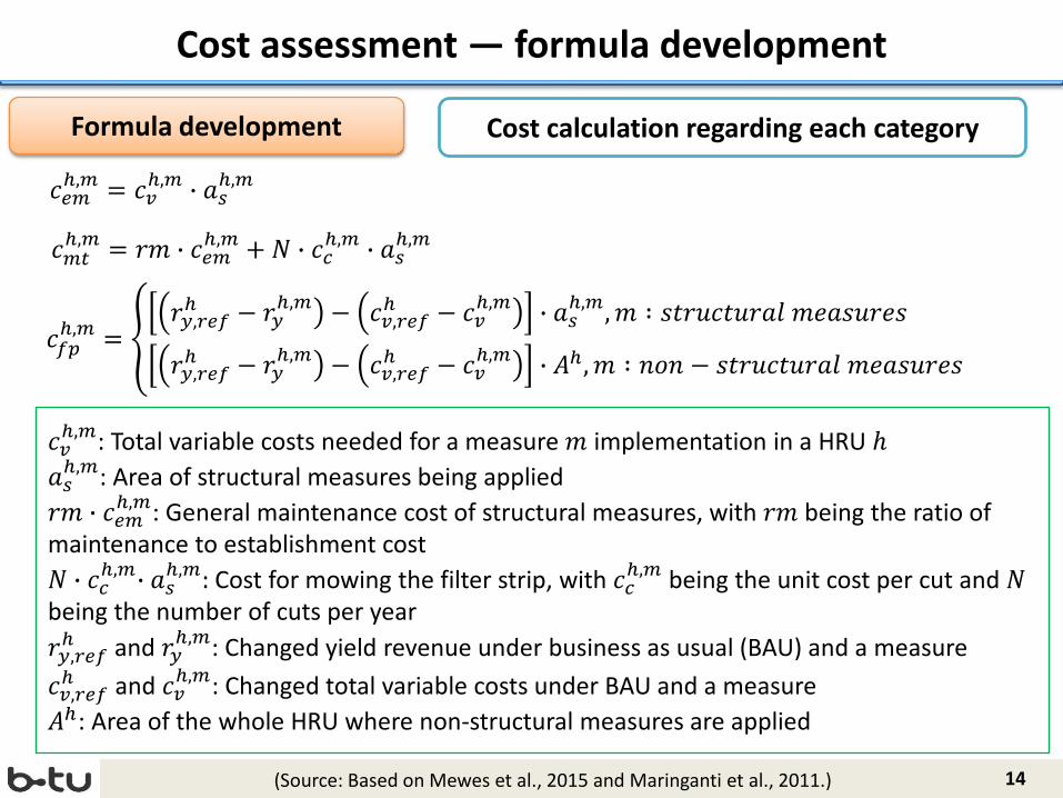
Cost assessment — formula development
Formula development Cost calculation regarding each category
𝑐𝑐𝑒𝑒𝑚𝑚ℎ,𝑚𝑚 = 𝑐𝑐𝑣𝑣
ℎ,𝑚𝑚 � 𝑎𝑎𝑠𝑠ℎ,𝑚𝑚
𝑐𝑐𝑚𝑚𝑚𝑚ℎ,𝑚𝑚 = 𝑟𝑟𝑟𝑟 � 𝑐𝑐𝑒𝑒𝑚𝑚
ℎ,𝑚𝑚 + 𝑁𝑁 � 𝑐𝑐𝑐𝑐ℎ,𝑚𝑚 � 𝑎𝑎𝑠𝑠
ℎ,𝑚𝑚
𝑐𝑐𝑓𝑓𝑓𝑓ℎ,𝑚𝑚 = �
�𝑟𝑟𝑦𝑦,𝑟𝑟𝑒𝑒𝑓𝑓ℎ − �𝑟𝑟𝑦𝑦
ℎ,𝑚𝑚 − �𝑐𝑐𝑣𝑣,𝑟𝑟𝑒𝑒𝑓𝑓ℎ − �𝑐𝑐𝑣𝑣
ℎ,𝑚𝑚 � 𝑎𝑎𝑠𝑠ℎ,𝑚𝑚,𝑟𝑟 ∶ 𝑠𝑠𝑠𝑠𝑟𝑟𝑠𝑠𝑐𝑐𝑠𝑠𝑠𝑠𝑟𝑟𝑎𝑎𝑠𝑠 𝑟𝑟𝑚𝑚𝑎𝑎𝑠𝑠𝑠𝑠𝑟𝑟𝑚𝑚𝑠𝑠
�𝑟𝑟𝑦𝑦,𝑟𝑟𝑒𝑒𝑓𝑓ℎ − �𝑟𝑟𝑦𝑦
ℎ,𝑚𝑚 − �𝑐𝑐𝑣𝑣,𝑟𝑟𝑒𝑒𝑓𝑓ℎ − �𝑐𝑐𝑣𝑣
ℎ,𝑚𝑚 � 𝐴𝐴ℎ,𝑟𝑟 ∶ 𝑛𝑛𝑛𝑛𝑛𝑛 − 𝑠𝑠𝑠𝑠𝑟𝑟𝑠𝑠𝑐𝑐𝑠𝑠𝑠𝑠𝑟𝑟𝑎𝑎𝑠𝑠 𝑟𝑟𝑚𝑚𝑎𝑎𝑠𝑠𝑠𝑠𝑟𝑟𝑚𝑚𝑠𝑠
𝑐𝑐𝑣𝑣ℎ,𝑚𝑚: Total variable costs needed for a measure 𝑟𝑟 implementation in a HRU ℎ𝑎𝑎𝑠𝑠ℎ,𝑚𝑚: Area of structural measures being applied 𝑟𝑟𝑟𝑟 � 𝑐𝑐𝑒𝑒𝑚𝑚
ℎ,𝑚𝑚: General maintenance cost of structural measures, with 𝑟𝑟𝑟𝑟 being the ratio of maintenance to establishment cost𝑁𝑁 � 𝑐𝑐𝑐𝑐
ℎ,𝑚𝑚� 𝑎𝑎𝑠𝑠ℎ,𝑚𝑚: Cost for mowing the filter strip, with 𝑐𝑐𝑐𝑐
ℎ,𝑚𝑚 being the unit cost per cut and 𝑁𝑁being the number of cuts per year𝑟𝑟𝑦𝑦,𝑟𝑟𝑒𝑒𝑓𝑓ℎ and 𝑟𝑟𝑦𝑦
ℎ,𝑚𝑚: Changed yield revenue under business as usual (BAU) and a measure𝑐𝑐𝑣𝑣,𝑟𝑟𝑒𝑒𝑓𝑓ℎ and 𝑐𝑐𝑣𝑣
ℎ,𝑚𝑚: Changed total variable costs under BAU and a measure𝐴𝐴ℎ: Area of the whole HRU where non-structural measures are applied
(Source: Based on Mewes et al., 2015 and Maringanti et al., 2011.)

15Chair of Environmental Economics
Cost assessment — Data source
Data sources
Questionnaire
SWAT model • Crop yield• Area• Distance
Internet search
(Source: Own results from SWAT.)
16
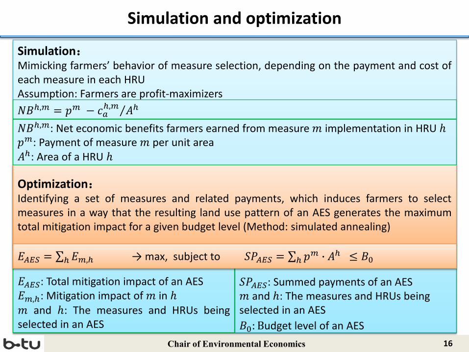
Simulation and optimization
Chair of Environmental Economics
Simulation:Mimicking farmers’ behavior of measure selection, depending on the payment and cost ofeach measure in each HRUAssumption: Farmers are profit-maximizers
Optimization:Identifying a set of measures and related payments, which induces farmers to selectmeasures in a way that the resulting land use pattern of an AES generates the maximumtotal mitigation impact for a given budget level (Method: simulated annealing)
𝐵𝐵0: Budget level of an AES
𝐸𝐸𝐴𝐴𝐴𝐴𝐴𝐴: Total mitigation impact of an AES𝐸𝐸𝑚𝑚,ℎ: Mitigation impact of 𝑟𝑟 in ℎ𝑟𝑟 and ℎ: The measures and HRUs beingselected in an AES
𝐸𝐸𝐴𝐴𝐴𝐴𝐴𝐴 = ∑ℎ𝐸𝐸𝑚𝑚,ℎ
𝑆𝑆𝑆𝑆𝐴𝐴𝐴𝐴𝐴𝐴: Summed payments of an AES𝑟𝑟 and ℎ: The measures and HRUs being selected in an AES
𝑆𝑆𝑆𝑆𝐴𝐴𝐴𝐴𝐴𝐴 = ∑ℎ 𝑝𝑝𝑚𝑚 � 𝐴𝐴ℎ𝐸𝐸𝐴𝐴𝐴𝐴𝐴𝐴 = ∑ℎ𝐸𝐸𝑚𝑚,ℎ → max, subject to 𝑆𝑆𝑆𝑆𝐴𝐴𝐴𝐴𝐴𝐴 = ∑ℎ 𝑝𝑝𝑚𝑚 � 𝐴𝐴ℎ ≤ 𝐵𝐵0
𝑁𝑁𝐵𝐵ℎ,𝑚𝑚 = 𝑝𝑝𝑚𝑚 − ⁄𝑐𝑐𝑎𝑎ℎ,𝑚𝑚 𝐴𝐴ℎ
𝑁𝑁𝐵𝐵ℎ,𝑚𝑚: Net economic benefits farmers earned from measure 𝑟𝑟 implementation in HRU ℎ𝑝𝑝𝑚𝑚: Payment of measure 𝑟𝑟 per unit area𝐴𝐴ℎ: Area of a HRU ℎ

17
Optimization modelling procedure
(Programmed by Dr. Astrid Sturm.)
18
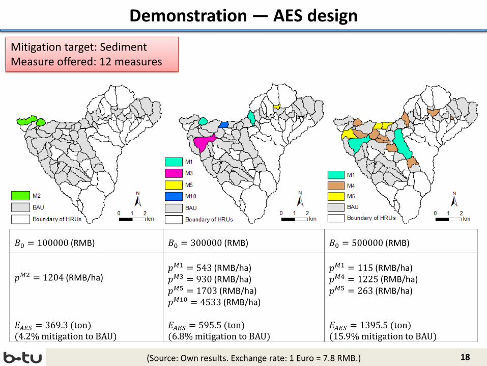
Demonstration — AES design
𝐵𝐵0 = 100000 (RMB)
Mitigation target: SedimentMeasure offered: 12 measures
𝑝𝑝𝑀𝑀2 = 1204 (RMB/ha)
𝐸𝐸𝐴𝐴𝐴𝐴𝐴𝐴 = 369.3 (ton)(4.2% mitigation to BAU)
𝐵𝐵0 = 300000 (RMB)
𝑝𝑝𝑀𝑀1 = 543 (RMB/ha)𝑝𝑝𝑀𝑀3 = 930 (RMB/ha)𝑝𝑝𝑀𝑀5 = 1703 (RMB/ha)𝑝𝑝𝑀𝑀10 = 4533 (RMB/ha)
𝐸𝐸𝐴𝐴𝐴𝐴𝐴𝐴 = 595.5 (ton)(6.8% mitigation to BAU)
𝐵𝐵0 = 500000 (RMB)
𝑝𝑝𝑀𝑀1 = 115 (RMB/ha)𝑝𝑝𝑀𝑀4 = 1225 (RMB/ha)𝑝𝑝𝑀𝑀5 = 263 (RMB/ha)
𝐸𝐸𝐴𝐴𝐴𝐴𝐴𝐴 = 1395.5 (ton)(15.9% mitigation to BAU)
(Source: Own results. Exchange rate: 1 Euro = 7.8 RMB.)

19Chair of Environmental Economics
Discussion and conclusion
Data limitation (SWAT model; cost assessment)
Cost components of measures (transaction costs; uncertainty costs)
Assumptions (HRUs are farms)
Developing a novel generic method
Considering spatial heterogeneity for both mitigation impacts and costs atthe same heterogeneous level
Designing the cost-effective measures allocation from perspective of AESdesign instead of top-down planning
Building an interdisciplinary research
Applying high technical and quantified research
20
Reference
• Boardman, A. E., Greenberg, D. H., Vining, A. R., & Weimer, D. L. (2017). Cost-benefit analysis: concepts and practice. Cambridge University Press.
• Mettepenningen, E., Verspecht, A., & Van Huylenbroeck, G. (2009). Measuring private transaction costs of European agri-environmental schemes. Journal of Environmental Planning and Management, 52(5), 649-667.
• Mewes, M., Drechsler, M., Johst, K., Sturm, A. and Wätzold, F. (2015), “A systematic approach for assessing spatially and temporally differentiated opportunity costs of biodiversity conservation measures in grasslands”, Agricultural Systems, Vol. 137, pp. 76–88.
• Wätzold, F., Drechsler, M., Johst, K., Mewes, M., & Sturm, A. (2016). A Novel, Spatiotemporally Explicit Ecological-economic Modeling Procedure for the Design of Cost-effective Agri-environment Schemes to Conserve Biodiversity. American Journal of Agricultural Economics, aav058.
• Wunder, S., & Wertz-Kanounnikoff, S. (2009). Payments for ecosystem services: a new way of conserving biodiversity in forests. Journal of Sustainable Forestry, 28(3-5), 576-596.
Chair of Environmental Economics
Chair of Environmental Economics