a novel method for intelligent fault diagnosis of bearing
TRANSCRIPT

Research ArticleA Novel Method for Intelligent Fault Diagnosis of Bearing Basedon Capsule Neural Network
Zhijian Wang 12 Likang Zheng 3 Wenhua Du 1 Wenan Cai 4 Jie Zhou 1
Jingtai Wang 1 Xiaofeng Han1 and Gaofeng He 1
1 School of Mechanical Engineering North University of China Taiyuan Shanxi 030051 China2School of Mechanical Engineering Xirsquoan Jiaotong University Shanxi 030619 China3School of Energy and Power Engineering North University of China Taiyuan Shanxi 030051 China4School of Mechanical Engineering Jinzhong University Jinzhong Shanxi 030600 China
Correspondence should be addressed to Wenhua Du dwhnuceducn andWenan Cai caiwenan0008linktyuteducn
Received 8 April 2019 Revised 17 May 2019 Accepted 3 June 2019 Published 20 June 2019
Academic Editor Diego R Amancio
Copyright copy 2019 Zhijian Wang et al This is an open access article distributed under the Creative Commons Attribution Licensewhich permits unrestricted use distribution and reproduction in any medium provided the original work is properly cited
In the era of big data data-driven methods mainly based on deep learning have been widely used in the field of intelligent faultdiagnosis Traditional neural networks tend to be more subjective when classifying fault time-frequency graphs such as poolinglayer and ignore the location relationship of features The newly proposed neural network named capsules network takes intoaccount the size and location of the image Inspired by this capsules network combined with the Xception module (XCN) isapplied in intelligent fault diagnosis so as to improve the classification accuracy of intelligent fault diagnosis Firstly the faulttime-frequency graphs are obtained by wavelet time-frequency analysis Then the time-frequency graphs data which are adjustedthe pixel size are input into XCN for training In order to accelerate the learning rate the parameters which have bigger changeare punished by cost function in the process of training After the operation of dynamic routing the length of the capsule is usedto classify the types of faults and get the classification of loss Then the longest capsule is used to reconstruct fault time-frequencygraphs which are used to measure the reconstruction of loss In order to determine the convergence condition the three losses arecombined through the weight coefficient Finally the proposed model and the traditional methods are respectively trained andtested under laboratory conditions and actual wind turbine gearbox conditions to verify the classification ability and reliable ability
1 Introduction
The rolling bearing is the most commonly used part inmechanical equipment In the working process the bearingmay be damaged due to improper assembly poor lubricationwater and foreign body invasion corrosion overload etc [1]Due to the processing technology working environment andother reasons the fault signal is nonlinear and nonstationarywhichmakes the dynamic mutation of the fault signal unableto be detected effectively So it is difficult to identify the faulttype of bearing accurately and stably Compared with othermachine parts the rolling bearing works badly which causesthe probability of failure to be high and the unpredictabilitystrong Therefore the fault diagnosis of rolling bearings is ofgreat significance to ensure the safety of equipment personalproperty and maintenance cost [2]
In recent years methods based on signal processing [3]or deep learning [4 5] are widely used to solve practi-cal engineering problems [6ndash9] Moreover in the field ofcompound fault diagnosis of rotating machinery with thecontinuous exploration of many researchers novel intelligentfault diagnosis methods emerge in an endless flow Forexample the methods based on the entropy [10 11] ofsignal processing includemaximumkurtosis spectral entropydeconvolution (MKSED) [12] multipoint optimal minimumentropy deconvolution adjusted (MOMEDA) [13] modifiedmultiscale symbolic dynamic entropy (MMSDE) [14] andminimum entropy deconvolution [15] In addition thereare other ways such as improved ensemble local meandecomposition (IELMD) [16 17] kernel regression residual[18] and modified variable modal decomposition (MVMD)[19 20] Methods based on big data and machine learning or
HindawiComplexityVolume 2019 Article ID 6943234 17 pageshttpsdoiorg10115520196943234
2 Complexity
deep learning include support vectormachine (SVM) [21 22]extreme learning machine (ELM) [23] kernel extreme learn-ing machine (KELM) [24] deep belief network (DBN) [25]and convolutional neural network (CNN) [26 27] In generalthese methods can solve most classification problems wellBut for composite fault diagnosis their fault test accuracyrate is not too high Moreover this kind of algorithm alwaysfails when there is not enough data to meet the convergencecondition or causes overfitting phenomenon which will leadto low test accuracy [28]
For example the traditional convolution neural networkrequires a lot of training samples to meet the convergencecondition Moreover people may subjectively reduce thedimension of filter [29] on the pooling of convolution neuralnetwork layer which can result in a substantial loss on thepooling layer information and even causes a phenomenonthat the input has a small change but the output is hardlychanged However as for time-frequency graphs a very smallchange may be the different type of bearing fault type orthe large change of fault size To summarize the traditionalconvolutional neural network is difficult to achieve a highfault test accuracy
Based on these disadvantages of traditional convolu-tional neural network the capsule neural network (CapsNet)architecture was proposed by Hinton and his assistants inNovember 2017 [30] which can retain the exact positioninclination size and other parameters of the feature inthe time-frequency graphs when training the deep learningmethod so as to make the slight changes in the input alsobring about slight changes in the output In the famoushandwritten digital image data set (Minst) CapsNet hasreached the most advanced performance of the current deeplearning algorithms CapsNeth architecture is made up ofcapsules rather than neurons A capsule is a small groupof neurons that can learn to examine a particular objectin an area of an image Its output is a vector the lengthof each vector represents the estimated probability of theexistence of the feature and its direction records the objectof attitude parameters such as accurate position inclinationand size If the feature changes slightly the capsule will outputa vector with the same length but slightly different directionwhich is helpful to improve the test accuracy of bearing faultdiagnosis
The input of the deep learning algorithm in the faultdiagnosis is fault time-frequency graphs and the two com-mon time-frequency analysis methods are short-time Fouriertime-frequency analysis and wavelet time-frequency anal-ysis Short-time Fourier transform (STFT) used to play adominant role in the field of signals and is an indispensableanalysis method [31] However due to its own limitations it isunable to deal with the nonstationary signals in real life andthere is a contradiction between noise suppression and signalprotection in the process of signal denoising After the ideaof wavelet transform the wavelet transform replaces the posi-tion of Fourier transform in signal processing Firstly wavelethas very good time-frequency characteristics and can decom-pose many different frequency signals in nonstationary sig-nals into nonoverlapping frequency bands which can solvethe problems encountered in signal filtering signal-noise
separation and feature extraction well [32] Secondly due tothe time-frequency characteristic of localization the choiceof wavelet basis is flexible and the calculation speed is veryfast whichmakeswavelet transformapowerful tool for signaldenoising Wavelet denoising can effectively remove noiseand retain the original signal thus improving the signal-to-noise ratio of the signal Therefore the continuous wavelettransform can effectively separate the effective part of thesignal from the noise greatly improve the feature extractionperformance of fault diagnosis [33] and finally improve thefault recognition rate
In addition improving the network structure canimprove the learning ability and reliable ability of the neuralnetwork For example using the Inception of modules andconvolution in GoogLeNet can help neural network indifferent areas to capture more target-oriented characteristicaccelerate the calculation speed and increase the depth ofthe neural network [34 35] Besides Xception module isthe extreme version of Inception [36] Xception modulecompletely decoupled across the channel correlation andspatial correlation and has achieved the classificationaccuracy of 945 in the classification of ImageNet database[37]
In terms of the convergence condition of the deep learn-ing algorithm most of them only consider the classificationloss as the only index of convergence and do not consider theinfluence on the model when the parameters change a lot orthe reconstruction loss which may make the model difficultto converge or require a lot of time to converge [38]Howevermost samples are collected under ideal working conditionsin the laboratory which may lead to the contingency whenverifying the feasibility of the deep learning method In otherwords this deep learning method can only diagnose thegearbox under the specificworking conditions [39 40] whichmeans that the reliably is very poor
Based on the above a novel intelligent fault diagnosismethod of capsules network combined with the Xceptionmodule was proposed and the weight coefficient of loss wastaken into account in order to improve the convergencespeed of the neural network classification robustness andlearning ability In order to verify XCNmodel of classificationability and reliable ability the ideal laboratory conditionof samples and the actual work condition of samples werechosen to train and test respectively and compare with otherdeep learning methods
2 The Basic Theory of the Model
21 Wavelet Transform and Time-Frequency TransformCompared with the short-time Fourier transform (STFT)method the wavelet basis of continuous wavelet transformis no longer a trig function of infinite length but a waveletbasis function of finite length that will decay The waveletbasis can be stretched which solves the problem that thetime resolution and the frequency resolution cannot be both[41] so it can better and effectively extract the effectiveinformation in the bearing fault time domain signal
Assuming the function 120593(119905) isin 1198712(119877) its Fourier trans-form 120593(120596) satisfies the condition
Complexity 3
119862120593 = intinfin0
1003816100381610038161003816120593 (120596)10038161003816100381610038162120596 119889120596 lt infin (1)
where the function 120593(119905) is called the parent wavelet or waveletbasis After scaling and shifting the parent wavelet a waveletfunction cluster can be generated whose expression is asfollows
120593119886119887 (119905) = 1radic119886120593(119905 minus 119887119886 ) (2)
where 119886 is the scale factor and 119887 is the translation factor Thescale factor 119886 is used to scale the wavelet basis while the scalefactor 119887 is used to change the position of the window on thetime axis
The continuous wavelet transform of the signal 119909(119905) isdefined as
119862119882119879 (119886 119887) = 1radic119886 intinfin
minusinfin119909 (119905) 120593 (119905 minus 119887119886 )119889119905 (3)
However most of the fault signals of the rolling bearingsare impulse fault signals whose time-domain waveform isdamped and freely attenuated vibration while the time-domain waveform feature of Morlet wavelet is vibrationattenuation from the central position to both sides Andtheir signals are similar [42 43] Therefore the Morlet ofcontinuous wavelet transform is selected as a wavelet basisand its function is as follows
120593 (119905) = 119890minus119905221198901198941205960119905 (4)
After determining the wavelet base and scale the actualfrequency sequence 119891 is combined with the time series todraw the wavelet time-frequency graphs
22 The Principle of Capsule Network Capsule network is anovel type of neural network proposed by Hinton and hisassistant in October 2017 which uses the module length ofthe activation vector of the capsule to describe the probabilityof the existence of the feature and uses the direction of theactivation vector of the capsule to represent the parametersof the corresponding instance [30]
Unlike previous neural networks which are composedof nerve neurons capsule neural networks are composedof many capsules with specific meanings and directionsActivation of neuronal activity within the capsule representsvarious properties of a specific feature presented in theimage These properties can include many different typesof instantiation parameters such as posture (position sizeand direction) deformation velocity reflectivity tone andtexture
At the network level the capsule neural network iscomposed of many layersThe lowest level capsules are calledvector capsules and they use only a small portion of theimage as input respectively The small area is called theperceptual domain and it attempted to detect whether aparticular pattern exists and how it is posed At higher levelscapsules called routing capsules are used to detect larger andmore complex objects
The output of the capsule is a vector the length of eachvector represents the estimated probability of the existenceof the object and its direction records the object of attitudeparameters If the object changes slightly the capsule will alsooutput a vector with the same length but slightly differentdirection So the capsules are isotropic For example ifthe capsule neural network outputs an eight-dimensionalcapsule its vector length represents the estimated probabilityof the existence of the object and its direction in the eight-dimensional space represents its various parameters such asthe exact position of the object or the number of rotationangles Then when the object rotates by a certain angle ormoves by a certain distance it only changes the directionof the output vector not its length so it has little effect onthe recognition rate of capsule neural network Moreoverthis phenomenon is not found in traditional neural networkssuch as convolutional neural networks
Convolution neural network such as the traditionalneural network mostly through pooling mechanisms whichchoose the maximum value of the region or in a fixed areaaverage extracts main features to next layers which makesthe neural network of subjectivity much bigger Thereforethe pooling operation may reduce the recognition rate of theneural network greatly The capsule neural network proposeda very significant mechanism called the dynamic routingmechanism In the capsule neural network the output ofthe capsule is set as a vector which makes it possible to usea powerful dynamic routing mechanism to ensure that theoutput of the capsule is sent to the appropriate parent nodein the above layer Initially the output is routed to all possibleparent nodes after the coupling sum is reduced by a factor of1 For each possible parent node the capsule calculates theprediction vector by multiplying its own output by a weightmatrix If the scalar product of this prediction vector andthe output of a possible parent node are larger than othersthere is top-down feedback which has the effect of increasingthe coupling coefficient of this parent node and reducing thecoupling coefficient of other parent nodes This increases thecontribution of the capsule to that parent node and furtherincreases the scalar product of the capsule prediction vectorand the output of that parent node So this operation is moreefficient than the primitive form of routing implementedthrough pooling where all feature detectors in the next layerare ignored except for the most active feature detectors inthe local layer In Hintons paper he demonstrated that [30]Then he imported the images inMinst into the capsule neuralnetwork with dynamic routing and the convolution neuralnetwork with pooling respectively finally finding the capsuleneural network in the digital recognition accuracy comparedto convolution neural network and capsule neural network issignificantly higher than the convolutional neural network onthe highly overlapping digital image recognition So dynamicrouting mechanism is a very effective way
Take a three-layer capsule neural network architecturefor identifying digital images in Minst which is shownin Figure 1 The architecture can be simply represented asconsisting of only two convolutional layers and one fullyconnected layer Conv1 is activated by 256 9times9 convolutionkernels stride 1 and ReLU function The layer converted the
4 Complexity
9times9
20
9times9
ReLU Conv1
6
Primary Caps
16
DigitCaps
10 10256
8
32
L2
WCD = [8 times 16]
Figure 1 Three-layer capsule neural network
Input
Concat
1times1Convolution
3times3Convolution
5times5Convolution
3times3Convolution
Figure 2 Inception module
pixel intensity into a matrix Then the matrix is used as theactivated part of the local feature detector input by the basiccapsuleThe length of the activation vector for each capsule inthe DigitCaps layer represents the probability of the specificobject and is used to calculate the classification loss119882119894119895 is a weight matrix for each input in the PrimaryCapsule and 1198712 is the length of the longest capsule
23 Xception Module In order to obtain a deeper featuregraph the traditional neural network tends to increase thenumber of layers of convolution which will bring too manyparameters and make it difficult to train More importantlyit increases the time and space consumption Moreover theconvolution kernel of the same layer in the traditional convo-lutional neural network is single but the correlation betweendifferent channels in the time-frequency graphs is not verymuch which requires the use of different convolution kernelfor different channels
To solve these problems Inception provides a differentway to extract deeper feature maps By using convolutionkernels of different sizes in the same layer different sizes ofsensing fields can be obtained to improve the classificationeffect Its architecture is shown in Figure 2
An input feature graph is processed by the convolutionkernel of 1times1 3times3 and 5times5 at the same time and theobtained features are combined which can extract manykinds of features and obtain better results However thereis a serious problem with this structure that the numberof parameters is much larger than that of using a single
convolution kernel and such a huge amount of calculationwill make the model inefficient This was inspired by the 1times1convolution kernel in the Network In Network 1times1 convolu-tion kernel is added to Inception Its architecture is shown inFigure 3
To take an example which is shown in Figure 4 assumingthat the dimension of the input feature graph is 256 theoutput dimension is also 256 There are two operations
The first is that the 256-dimensional input goes througha convolution layer of 3times3times256 directly And the output is a256-dimensional feature graph so the number of parametersis 256times3times3times256=589824
The second is that firstly the 256-dimensional inputpasses through a convolution layer of 1times1times64 then througha convolution layer of 3times3times64 and finally through aconvolution layer of 1times1times256 The output dimension is256 but the number of parameters is 256times1times1times64+64times3times3times64+64times1times1times256=69632 That reduces the number ofparameters for the first operation to one in nine
For convolution the convolution kernel can be viewedas a three-dimensional filter channel dimension and spatialdimension (width and height of the feature graph) Theconventional convolution operation is actually the joint map-ping of channel correlation and spatial correlation Incep-tion module is based on the assumption that the channelcorrelation and spatial correlation between the channels inthe convolutional layer can be decoupled So mapping thechannel correlation and spatial correlation can get betterresults separately
Complexity 5
Input
1times1Convolution
Concat
1times1Convolution
1times1Convolution
1times1Convolution
3times3Convolution
5times5Convolution
3times3Convolution
Figure 3 Inception module with 1times1 convolution
Output 256dim3times3times256Input
256 dim
Output 256 dim1times1times2563times3times641times1times64Input
256 dim
SecondProcess
First process
Figure 4 Comparison of the convolution process with and without 1times1 convolutionBased on the Inception hypothesis it can be found that
when the number of channels increases it is more reasonableto assume that cross-channel correlation and spatial correla-tion mapping are completely separated
Based on the above findings and assumptions the Xcep-tion module was proposed Firstly it uses 1x1 convolutionmap to map cross-channel correlation and then there isan independent spatial convolution on each output channelof 1times1 convolution to map spatial correlation The channelcorrelation convolution of 1times1 is carried out and the numberof convolution kernels with different types of subsequentconvolving is the same as the number of output channelsof 1times1 convolution Various feature maps are output duringthe whole Xcepiton module process and each output can berepresented by the following function
119909119897119895 = 119891 (119906119897119895) (5)
119906119897119895 = sum119894
119909119897minus1119894 times 119908119897119894119895 + 119887119897119895 (6)
where 119909119897119895 is the output of the convolution channel 119897 of theconvolution layer 119895 119906119897119895 is the net activation of the convolutionchannel 119897 of the convolution layer 119895 119908119897119894119895 is the weightcoefficients between the layer 119894 and the layer 119895 and 119887119897119895 is thethreshold offset term of the channel 119897 of the convolution layer119895
Then all outputs are connected together through a fullconnection operation its function is as follows
119909119897 = 119891 (119906119897) (7)
119906119897 = 119908119897119909119897minus1 + 119887119897 (8)
And the gradient descent method is used to reduce the errorof the whole process its function is as follows
nabla120593 (119906119897) = 120597120593120597119906119897 (9)
where nabla120593(119906119897) is the error 120593(119906119897) with the changing of 119906119897Although the architecture of the Xception module is
basically the same as Inception the improvement of Xceptionmodule performance is not due to the increase of modelcapacity but due to the more efficient use of model param-eters
Because the parts of the image with a long distance do notmatter much different convolution kernels are adopted in theXception module Inspired by convolution decompositionit is used for different convolution kernels For examplethe 7times7 convolution kernels are decomposed into two one-dimensional convolution kernels 1times7 and 7times1 And the3times3 convolution kernel is same for two one-dimensionalconvolution kernels 1times3 and 3times1 Such operation can notonly accelerate the calculation but also further increase thenetwork depth which is helpful to improve the learningability of the neural network This is because what is usefulis the homology of the information not the invariance andthe sorting of the information rather than the discardingof the information In addition it also routes every part ofthe input into neurons that know how to process it whichmeans finding the best path However pooling operationdetermined by human factors performs poorly in handlingdynamic routing so it is not good for the establishment ofneural network
6 Complexity
Concat
1times1Convolution
Input
1times1Convolution
Output Channel
1times3Convolution
1times5Convolution
1times7Convolution
1times3Convolution
3times1Convolution
5times1Convolution
7times1Convolution
3times1Convolution
Figure 5 Xception module
Building an improved Xcepiton module without poolinglayer is shown in Figure 5
3 Establishment of a Novel Capsule NeuralNetwork with Xception Module (XCN)
31 Input and Dynamic Routing of Capsule Neural NetworkWhen the time-frequency graphs of bearing fault are rec-ognized by the capsule neural network the selection of thestructure parameters of the capsule neural network has asignificant influence on the recognition results Thereforeonly when the appropriate parameters are selected can theclassification and recognition performance of the capsuleneural network for bearing faults be truly reflected Theinput of the capsule neural network is time-frequency graphswhose size can be chosen as a variety of sizes In this paperfor the sake of simplicity the pixel size of all time-frequencygraphs was chosen as 256times256 Then multiple normal time-frequency graphs and failure time-frequency graphs wereimported into the XCN model
The length of the output vector of the capsule was usedto represent the probability that the entity represented by thecapsule exists in the current input In addition a nonlinearsquashing function was used to ensure that the short vectoris compressed to nearly 0 and the long vector is compressedto slightly less than 1
V119895 =1003816100381610038161003816100381610038161003816100381610038161003816119904119895100381610038161003816100381610038161003816100381610038161003816100381621 + 100381610038161003816100381610038161003816100381610038161003816100381611990411989510038161003816100381610038161003816100381610038161003816100381610038162
11990411989510038161003816100381610038161003816100381610038161003816100381610038161199041198951003816100381610038161003816100381610038161003816100381610038161003816 (10)
where V119895 is the vector output of the capsule 119895 and 119904119895 is its totalinput
In addition to the first layer of the capsule body the totalinput 119904119895 of the capsule is a weighted sum of the predictionvector 119906119895|119894 of all the capsules from the next layer which isgenerated by multiplying the output 119906119894 of the following layerof capsules by the weight matrix119882119894119895
119904119895 = sum119894
119888119894119895 and119906119895|119894 (11)
119888119894119895 = exp (119887119894119895)sum119896 exp (119887119894119896) (12)
and119906119895|119894 = 119882119894119895119906119894 (13)
where 119888119894119895 is the coupling coefficient determined by theiterative dynamic routing process The sum of couplingcoefficients between the capsule 119894 and all capsules in thehigher layer is 1 which is determined by routing softmaxTheinitial logic 119887 119894119895 of routing softmax is the logarithmic priorprobability that is the capsule 119894 should be coupled with thecapsule 119895 The logarithmic prior probability of the same timecan be used as the discriminant learning of all other weightsThey depend on the location and type of the two capsulesnot on the current input image Then the initial couplingcoefficient achieves iterative refinement by measuring theconsistency between the current output V 119895 of each capsule119895 in the higher layer and the predicted 119906119895|119894 of the capsule 119894Consistency is the index dot product 119886 119894119895 = V 119895 times 119906119895|119894 Thisconsistency is considered to be a logarithmic likelihood ratioand is added to the initial logic 119887 119894119895 before new values arecalculated for all coupling coefficients between capsule 119894 andhigher level capsules
In the convolutional capsule layers each capsule outputsa vector local network to each type of capsule in the higherlayer and uses a different transformation matrix for each partof the network and each type of capsule
This operation which Hinton calls dynamic routingbetween capsules is used in the propagation of Primary capslayer toDigital caps layer Figure 6 shows the dynamic routingmechanism
Details of dynamic routing algorithm are shown in Pro-cedure 1
32 Output Vector Processing Method The time-frequencygraphs are imported into the XCN model Finally capsulevectors with many different meanings are obtained Themodules of all capsule vectors are calculated and the corre-sponding fault type of the capsule vector with the maximummodule value is obtained
Complexity 7
(1) procedure Routing (and119906119895|119894rl)(2) for all capsule i in layer l and capsule j in layer(l+1) 119887ij larr997888 0(3) for r iterations do(4) for all capsule i in layer l 119888i larr997888 119904119900119891119905119898119886119909(119887119894)(5) for all capsule j in layer(l+1) 119904119895 larr997888 sum119894 119888119894119895 and119906119895|119894(6) for all capsule j in layer(l+1) V119895 larr997888 119904119902119906119886119904ℎ(119904119895)(7) for all capsule i in layer l and capsule j in layer(l+1) 119887ij larr997888 119887ij + and119906119895|119894V119895return V119895
Procedure 1 Routing algorithm
Capsule i Capsule j
Upper layersPrevious layers
Wij cij
Figure 6 Dynamic routing mechanism
In order to know the fault identification rate of XCNmodel intuitively the specific capsules are generated faulttime-frequency graphs through reconstruction In the pro-cess of training all the vectors in the Digital Caps layer exceptthe correct capsule vector are shielded that is only the correctcapsule is kept and the other capsules are set to zeroThen theDigital Caps layer is used to reconstruct the input graph Theoutput of the digital capsule is fed into a decoder composedof three inverse routing iterations which are formed of thefull connection layer and the linear unit activation function isadded in each layer of the full connection layer to ensure thatthe feature graph of the output of each layer is positive Thenthe original fault time-frequency graph and the reconstructedfault time-frequency graph are fused into a 256times256 targetgraph The reconstructed flow chart is shown in Figure 7
In order to measure the difference between reconstructedgraph and truth graph in texture details and structure andminimize the loss of texture details and structure informationof reconstructed graph in this paper the reconstruction lossfunction of XCNmodel uses1198712 norm tomeasure the distancebetween reconstructed graph and truth graphThe formula is
119897120574 = 119889 (119866 (119885) minus 119885)119885 = 119866 (119885) minus 1198852119885 (14)
where119885 represents the input original graph 119866(119885) representsthe reconstructed graph and 119897120574 represents the reconstructionloss
33 Adjustment of Capsule Neural Network Cross entropymeasures the difference information between two probability
distributions by describing the distance between them Themethod of capsule neural network to solve the multiclassi-fication problem is to set output capsules 119899 where 119899 is thenumber of categories and each capsule represents a differentcategory For each sample an n-dimensional array formedof the length of each output capsule can be obtained bythe capsule neural network Each dimension in the arraycorresponds to a category Ideally if a sample belongs to thecategory 119896 the output value of the output node correspondingto that category should be 1 while the output value of all othernodes should be 0
Take an example of identifying handwritten Numbers inMinst which fall into 10 categories from 0 to 9 When thenumber 1 is recognized the closer the output 10-dimensionalarray of the capsule neural network [0 1 0 0 0 0 0 0 0]the better The ideal probability distribution on handwrittennumber classification is defined as 119901(119909) and the probabilitydistribution of the output of the capsule neural network as119902(119909) Then the cross entropy of this sample classification is
119867(119901 119902) = minussum119901 (119909) times log10 119902 (119909) (15)
The cross entropy represents the uncertainty of the randomvariable or the whole system The higher the entropy isthe greater the uncertainty of the random variable or thewhole system will be However cross entropy describes thedistance between two probability distributions While theoutput length of the capsule neural network is not necessarilya probability distribution nor is necessarily between 0 and1 softmax regression is a very useful way to transform theresults of the forward propagation of the capsule neuralnetwork into a probability distribution
Assuming the output of the neural network is 1199101 1199102 1199103sdot sdot sdot 119910119899 the output after softmax regression processing is
119904119900119891119905119898119886119909 (119910)119894 = 1199101015840119894 = 119890119910119894sum119899119895=1 119890119910119895 (16)
Softmax transformed the output of the capsule neuralnetwork into a probability distribution In thisway the outputof the capsule neural network is also turned into a proba-bility distribution and the distance between the predictedprobability distribution and the actual answer probabilitydistribution can be calculated by cross entropy
8 Complexity
DigitCaps10 9times9
9times9
ReLu ReLu Somax
16
Figure 7 Reconstruction mechanism
Then the cross entropy loss function of the capsule neuralnetwork is
119867(119901 119910) = minus 119899sum119894
119901 (119909119894) times log10 119910119894 (17)
where 119909119894 is its correct output 119901(119909119894) is its probability and 119910119894 isthe actual probability
In the neural network the minimal fluctuation of someparameters of weights will often lead to the change of thevalue of the loss function which will lead to the overfittingof the model or the long convergence time which will affectthe prediction performance In order to improve this phe-nomenon the 1198712 norm is introduced as the punishment forthe parameters whose weight changes greatly each time thestructure of the capsule neural network is adjusted 1198712normrefers to the sum of squares of the weight of ownershipdivided by the number of samples The expression is asfollows
1205792 = radic 119896sum119896=1
119897sum119897=1
1205792119896119897 (18)
where 120579119896119897 is the weight of the parameter 119897 in the layer 119896Then combine the loss function penalty function of the
XCN model and the reconstruction loss in the reconstruc-tion through the regularization term coefficient 120572 and 120573 sothat when the gradient of the adjustment function 119871 reachesthe minimum value it can be considered that the capsuleneural network has been convergent The expression of theadjustment function 119871 of the capsule neural network is asfollows
119871 = 119867(119901 119910) + 120572 12057922 + 120573119897120574 (19)
where 119871 is the adjustment function of the capsule neuralnetwork119867(119901 119910) is the loss function 120572 and 120573 are the weightcoefficients 12057922 is the square of the penalty function and 119897120574is the reconstruction loss
In order to ensure the accuracy of the classificationand avoid over-fitting during training 120572 and 120573 should beappropriately selected For example the size of 119867(119901 119910) and12057922 is between 0 and 1 If the loss function is set in a largeproportion it will lead to the nonconvergence of the trainingprocess of the capsule neural network If the penalty functionis set in a large proportion it will lead to the low accuracy
of classification Therefore the weight coefficient 120572 must beset a series of values and then test its performance andadjust through experiments Similarly the selection of theweight coefficient 120573 also needs to go through the appropriateselection
The flowchart of XCN model is shown in Figure 8
34 Feasibility Discussion of XCN Model When the XCNmodel is used to identify bearing fault signals the time-domain signals collected by the sensor need to be convertedinto time-frequency graphs In the process of fault time-frequency graphs processing the signal noise reduction andfeature extraction are carried out firstly And then the time-frequency graphs with pixel adjustment are taken as theinput of the capsule neural network In this paper a capsuleneural network was established with a convolutional layera dynamic routing layer a full connection layer and areconstructed decoder In order to improve the depth anddimension of the neural network the Xception module wasadded to the neural network to improve the fault classificationaccuracyWhen using XCNmodel to identify time-frequencygraphs different parameter settings have a great impacton the identification results of the capsule neural networkincluding the number of iterations batch size size andnumber of convolution kernels the number of layers ofXception module the selection of convolution parametersand the weight coefficient In order to discuss the feasibilityof the XCN model the bearing failure data set provided byCase Western Reserve University was used to train and testthe XCN model Figure 9 shows the experimental station ofCase Western Reserve University All the algorithm programcode was written in and run on a computer with CPUi7-4790K400GHz RAM 1600G GPU Nvidia GeforceGTX960 and operating systemWin7
The experiment was carried out with a 2 HP motor andfan end bearing data was all collected at 12000 samples persecond and the acceleration data were measured near andaway from the motor bearing In this data set all the dataare from the bearings damaged by the test bench In otherwords the load of each bearing is the same (in this papertest bearing data under no-load condition was selected)but the health condition of the bearing is different For theacquisition of faulty bearings three different kinds of damagewere caused to the outer ring inner ring or balls of thebearing by electrical discharge machining and their failurediameter was selected for a class of test bearing data sets of
Complexity 9
Training XCN
Testng XCN
Increase the number of training samples
Map to Xception calculation
Calculate the adjustment function gradient
Input sample completed
Meet the iteration termination condition
Classification amp reconstruction
Map to the convolution layer
Dynamic routing amp fully connecting
Data acquisition
Rolling bearing test
Fetch initial data
Time-frequency transformation
XCN aer training
Fault diagnosis Result amp analysis
Test sampleIntelligent fault diagnosis
Y
N
Y
N
8
6
4
2
0
minus2
minus4
minus60 02
005 01501 02
04 06 08 1 12 14 16 18 2
5
6
4
3
2
1
5
4
3
2
1
00
005 01501 02
5
6
4
3
2
1
5
4
3
2
1
00
Figure 8 Intelligent fault diagnosis flow chart based on XCN
0007 inches Therefore there are 4 types of time-frequencygraphs of bearings including the healthy bearings
In view of the rich information contained in the time-frequency graphs and the fact that the input of the cap-sule neural network must be a two-dimensional matrixwhen studying the fault identification performance of theXCN model time-frequency conversion processing of time-domain signals is required firstly In this paper the time-frequency conversion method is chosen as the continuouswavelet transform and thewavelet basis is theMorletwavelet
One sample of four different types in the data set is takenout for continuous wavelet transform respectively and theresults are shown in Figure 10
In order to reduce the influence of noise the zero meannormalization method was adopted which not only ensuresthe distribution of the original signal but also eliminates theinfluence of dimension and converts the data into the samedistribution The formula is as follows
119909lowast = 119909 minus 120583120590 (20)
10 Complexity
Figure 9 Experimental station of CaseWestern Reserve University
where 119909 is the input 119909lowast is the output of the time-frequencygraph and 120583 and 120590 are the mean and variance of 119909respectively
The input time-frequency graphs pixel size of bearingfailure was selected as 256times256 The selection of capsulevector should be carried out first when the time-frequencygraphs with appropriate pixel adjustment are imported intothe capsule neural network for training In this paper thetonal distribution of time-frequency graphs and its changespeed and direction are selected to transform the character-istics Eighty percent of the samples from bearing data setprovided by CaseWestern Reserve University were randomlyselected for training to select parameters and twenty percentof the samples were tested to verify the reliability of theselected parameters
(1) Selection of Batch Size Batch size refers to the processof training the neural network in which a certain numberof samples are randomly selected for batch training eachtime Then the parameters of weight are adjusted once untilall training samples are input This process is called thecompletion of an iteration If a larger batch size value isselected the memory utilization can be improved throughparallelization so as to improve the running speed Inother words the convergence speed will be faster but thetimes of adjusting the weight will be less thus reducing theclassification accuracy While choosing a smaller batch sizecan improve classification accuracy it will lead to longercomputing time Therefore in the case of limited memorycapacity when selecting the batch size the requirementsof classification accuracy and computing time should beweighed to ensure that the time cost can be reduced asmuch as possible under the premise of sufficient classificationaccuracy The selection principle of batch size number mustfirst meet the requirement that the number of trainingsamples can be dividedTherefore the selected batch sizes are2 4 5 8 10 20 25 30 and 50 respectively When discussingthe influence of batch size on classification results in orderto simplify the complexity of the discussion the preliminaryassumption of the number of iterations is 10 the preliminaryassumption of the convolution kernel is 3times3 5times5 and 7times7whose number is 1 respectively and the weight coefficientis 04 and 06 respectively The experiment was repeated forten times and the average value of the classification resultsof ten times was taken as the final classification accuracyThen the relationship between the classification accuracy and
batch size was shown in Figure 11 As can be seen fromFigure 11 when the batch size is within 10 the change of thebatch size has little influence on the classification accuracywhile when the batch size is larger than 10 the classificationaccuracy obviously decreases with the increase of the batchsize As a result the total sample batch size mustmeet the firstcondition that it can be divided exactly by the training samplein certain cases Secondly choosing the smaller batch size canincrease the recognition rate of fault which contributes to thefailure of judgment Such as the trial when the batch size isselected as 5 8 10 or 20 the classification accuracy is thehighest Combined with the time cost factor the batch sizewas selected as 20
(2) Selection of Iteration Times In essence iteration isa process of continuous approximation and fitting If thenumber of iterations is too small the fitting effect will benot ideal When the number of iterations increases to acertain degree the fitting error will no longer decreasebut the time cost will increase with the increase of thenumber of iterations Therefore it is necessary to selectan appropriate number of iterations which can achieve arelatively low time cost under the condition of satisfying acertain recognition rate When discussing the influence ofiteration times on classification results in order to simplifythe complexity of discussion the batch size is selected as 20according to the previous section the convolution kernel ispreliminarily assumed to be 3times3 5times5 and 7times7 whose numberis 1 respectively and the weight coefficients are 04 and 06respectively The experiment was repeated for five times andthe average of the five classification results was taken as thefinal classification accuracy And the relationship betweenthe classification accuracy and the number of iterations isshown in Figure 12 As can be seen from Figure 12 withthe increase of iteration times the classification accuracyincreases gradually When the number of iterations reached6 the classification accuracy was more than 96 when thenumber of iterations was more than 10 the classificationaccuracy was more than 985 and with the increase of thenumber of iterations the classification accuracy tended tobe stable Therefore under the conditions of the number ofsamples and the size of graphs in this paper the selectionof 10 iterations can not only meet the requirements of highclassification accuracy but also reduce the time cost
(3) Selection of the Size and Quantity of Convolution KernelThe larger the size of the convolution kernel is the largerthe representable feature space of the network will be andthe stronger the learning ability will be However there willbe more parameters to be trained and the calculation willbe more complex which will lead to the phenomenon ofoverfitting easily Meanwhile the training time will be greatlyincreased 1times1 convolution can increase across the channelcorrelation to improve the utilization rate of XCN modelparameters which can be used in the Xception module butdoes not make sense in the feature extraction As the size ofan even number of convolution kernels even symmetricallyfor zero padding operations there is no guarantee that theinput graph size and output characteristics graph size remain
Complexity 11
0 5 10 15 20Time t (s)
100
200
300
400
500
600
700
Freq
uenc
y f (
Hz)
(a) Inner ring fault
5 10 15 20Time t (s)
100
200
300
400
500
600
700
Freq
uenc
y f (
Hz)
(b) Outer ring fault
0 5 10 15 20Time t (s)
100
200
300
400
500
600
700
Freq
uenc
y f (
Hz)
(c) Ball fault
0 5 10 15 20Time t (s)
100
200
300
400
500
600
700
Freq
uenc
y f (
Hz)
(d) Health
Figure 10 Signal time-frequency graphs of the experimental station of CaseWestern Reserve University
2 4 5 8 10 20 25 30 50Batch size
89
90
91
92
93
94
95
96
97
Clas
sifica
tion
accu
racy
()
Relationship between classification accuracy and batch size
Figure 11 Relationship between classification accuracy and batch size
12 Complexity
0 5 10 15 200
20
40
60
80
100
Clas
sifica
tion
accu
racy
()
Relationship between classification accuracy and iteration times
Iteration times
Figure 12 Relationship between classification accuracy and itera-tion times
the same In order to ensure that the size of the input andoutput characteristics graph is changeless the convolutionkernel size is chosen as the positive odd except 1 In the caseof reaching the same receptive field the smaller the size ofthe convolution kernel the faster the operation To simplifythe complexity of the discussion the maximum convolutionkernel is selected as 9times9 the number of different convolutionkernels is selected as 3 and the number of a single convo-lution kernels is no more than 2 The size and number ofconvolution kernels of each convolution layer constitute a setof parameters in which the optimal combination will largelydetermine the performance of the neural network The batchsize is selected as 20 according to the previous section thenumber of iterations is 10 and the weight coefficient is 04and 06 respectively The experiment was repeated for fivetimes and the average value of the five classification resultswas taken as the final classification accuracyThe relationshipbetween the classification accuracy and the size and quantityof the convolution kernel is shown in Figure 13 In Figure 13357 represents the convolution kernel combination of 3times35times5 and 7times7 And label 1-2-1 indicates that in the convolutionkernel combination the number of the first convolutionkernel is 1 the number of the second convolution kernel is2 and the number of the third convolution kernel is 1 Andthe same is true for other labels According to Figure 13when the combination of convolution kernels is 357 overallclassification accuracy is higher than other combination Inaddition in the combination of 357 and label is 2-2-1the classification accuracy reaches 989 which shows thatthe 3times3 5times5 and 7times7 convolution kernels are better thanother combinations to extract features Furthermore in theconvolution kernels combination of 3times3 and 5times5 is able toextract features more than 7 x 7 convolution kernels
(4) Selection of Weight Coefficients 120572 and 120573 The weight valueof the weight coefficient 120572 represents the size of the degreeof punishment on the XCN model when the parametersare adjusted every time And choosing the appropriateweight coefficient 120572 can enhance the robustness of the XCN
357 379 359 579e number of convolution kernels and the number of dimensional iterations
70
75
80
85
90
95
100
Clas
sifica
tion
accu
racy
()
Relationship between classification accuracy and the numberof convolution kernels and the number of dimensional iterations
1-1-12-1-11-2-11-1-22-2-12-1-21-2-22-2-2
Figure 13 Relationship between classification accuracy and thenumber of convolution kernels and the number of dimensionaliterations
model The weight of the weight coefficient 120573 indicates theproportion of reconstruction loss And choosing the appro-priate weight coefficient 120573 can enhance the classificationaccuracy of XCN model The loss function 119867(119901 119910) thepenalty function 12057922 and the reconstruction loss 119897120574 are allfrom 0 to 1 because it reduces the impact of dimensionalityso the range of the weight coefficients 120572 and 120573 is selectedto be from 0 to 1 In order to simplify the complexity of thediscussion the weight coefficients 120572 and 120573 are reserved as onedecimal place According to the above section the batch sizeis selected as 20 the number of iterations is selected as 10the convolution kernel combination is selected as 357 andthe quantity allocation is selected as 2-2-1 The experimentwas repeated for five times and the average value of theclassification results of five times was taken as the finalclassification accuracy Then the relationship between theclassification accuracy and the weight coefficient is shown inFigure 14 It can be seen from Figure 14 that with the increaseof 120572 the classification accuracy tends to increase With theincrease of 120573 the classification accuracy first increases andthen decreases When the selection 120572 is 07 and 120573 is 06 theclassification accuracy reaches 985 while the classificationaccuracy of XCN is the highest
In order to verify the reliability of the selected parametersthe parameters of the XCN model are selected accordingto the above conclusions as follows batch size 20 iterationnumber 10 convolution kernel combination 357 quantityallocation 2-2-1 and weight coefficients 07 and 06 respec-tively The test was repeated for ten times and the test resultsare shown in Table 1
As can be seen from Table 1 under the selected XCNmodel parameters when the time-frequency graphs of three
Complexity 13
Table 1 Training accuracy and test accuracy of each type of fault
The fault types Average accuracy of training sample set () Average accuracy of test sample set ()Inner ring fault 998 992Outer ring fault 100 997Ball fault 985 963
201 09
40
08 1
60
07 09
Clas
sifica
tion
accu
racy
()
06 08
Relationship between classification accuracy and weight coefficients and
80
0705 0604 05
100
03 040302 0201 010
is 07 is 06
8 07 0 6 0 80 7
is 07 is
Figure 14 Relationship between classification accuracy and weight coefficients 120572 and 120573kinds of fault signal were identified the test accuracy andthe training accuracy are similar And the diagnosis accuracyis 963 in the diagnosis of outer ring fault which may berelated to time-frequency methods samples or other issuesand the rest were over 99 which shows the reliability ofparameter selection and XCN feasibility of the model
35 Reliably of the XCN Model
Experiment 1 (the test bearing data set of Western ReserveUniversity) In order to verify the superiority of the pro-posed method the XCN model proposed in the previoussection is compared with other deep learning algorithmsfor nearly three years DWAE+ELM [23] which is based ondeep wavelet autoencoder with extreme learning machineCapsNet which is based on standard capsule neural net-work MPE+ISVM+BT [22] which is based on multiscalepermutation entropy and improved support vector machinebased binary tree AE+ES+CNN [26] which is based onan acoustic emission analysis-based bearing fault diagno-sis invariant under fluctuations of rotational speeds usingenvelope spectrums and a convolutional neural network andDBN [25] which is based on the standard deep belief networkFinally the test accuracy of each algorithm is shown inTable 2and Figure 15
As can be seen from Table 2 and Figure 15 the faultdiagnosis accuracy of these six models in the bearing data settested by the Western Reserve University is generally higherthan 90 and the diagnostic accuracy of XCN model issignificantly higher than the other models The recognitionrates of XCN model in outer ring fault inner ring faultand ball fault are 992 997 and 963 respectivelyBy comparing XCN model with CapsNet it can be seen
that the former has higher diagnostic accuracy than thelatter in the three fault types which proves that Xceptioncan help improve the classification accuracy of CapsNet Bycomparing XCN model with the other four models exceptin the outer ring fault diagnosis the classification accuracyof SVM is 100 higher than XCN and the classificationaccuracy of XCN is all higher than other methodsThereforeit can be preliminarily concluded that XCN has certainadvantages over other methods in bearing fault diagnosis
Experiment 2 (the test bearing data set of wind turbine gear-box in actual working conditions) For gearbox under theactual working conditions there are always somemechanicalworking changes such as speed and load Due to the lackof reliable ability these deep learning methods can only beeffective under conditions similar to training data In otherwords these methods may fail if the working condition of thegearbox changes
In order to discuss the reliability of the XCN modeland compare it with other deep learning methods theywere imported to the samples obtained from the windturbine gearbox under actual working conditions to trainand testTable 3 is the parameters of a wind turbine gearboxunder actual working conditions
Figure 16 is a real picture of three faults of a wind powergearbox The sampling frequency is 5333Hz and the gearboxtransmission ratio is 1134 The three fault types of windturbine gearbox are shown in Figure 16
Firstly the collected time-domain signals were trans-formed into time-frequency graphs through continuouswavelet time-frequency transformation Secondly the time-frequency graphs were imported into the XCN model afteradjusting the pixel size Finally the same input was imported
14 Complexity
Inner ring fault Outer ring fault Ball fault85
90
95
100
XCNDWAE+ELMCapsNetMPE+ISVM+BTAE+ES+CNNDBN
Figure 15 Average classification accuracy of different algorithms based on the test bearing data set of Western Reserve University
Table 2 Average classification accuracy of different algorithms
Average accuracy oftest sample set () XCN DWAE+ELM CapsNet MPE+ISVM+BT AE+ES+CNN DBN
Inner ring fault 992 952 956 964 954 931Outer ring fault 997 952 953 100 926 943Ball fault 963 952 919 964 922 893
Table 3 Parameters of wind power gearbox under a certain actual working condition
Parameters of a wind power gearbox (including three planetary wheels)Part name Number of teeth Rotate speed (rmin)Wind turbines 92The ring gear 92 0The planets gear 37 -2378The sun gear 16 108Intermediate gear 91 108Intermediate gear shaft 20 4914Final big gear 96 4914Output gear shaft 26 18144
into other algorithms such as DWAE+ELM [23] CapsNetMPE+ISVM+BT [22] AE+ES+CNN [26] and DBN [25] andtested the failure diagnosis performance of these methods
In this experiment sixty percent of the adjusted time-frequency graphs were used for algorithm training and fortypercent were used for testing The experiment was repeatedfive timesTable 4 and Figure 17 show the fault identificationrates of the three algorithms
It can be seen from Table 4 and Figure 17 that XCNmodel in these kinds of fault identification is obviouslybetter than the other methods In addition XCN model inthe recognition rate of outer ring fault and inner ring faultreached 987 and 972 respectively but the recognitionrate of tapered roller fault is only 945 which may bebecause the noise is too large and the time-frequency method
is poor By comparing the fault identification rates of thesealgorithms it can be seen that the XCN model has greatadvantages in the fault identification of the wind turbinegearbox Moreover combined with the experiment in theprevious section it can be shown that the XCN model hasa certain reliable ability rather than being limited to theworking environment of the laboratory
4 Conclusion
This paper takes the intelligent diagnosis of bearing faultsas the research object combines the capsule neural networkwhich belongs to the category of deep learning with theXception module and then applies it to the fault identifica-tion of the wind turbine gearbox Firstly the time-domain
Complexity 15
Table 4 Average classification accuracy of different algorithms
Average accuracy of testsample set () XCN DWAE+ELM CapsNet MPE+ISVM+BT AE+ES+CNN DBN
Inner ring fault 972 886 956 876 904 891Outer ring fault 987 913 943 903 926 913Tapered roller fault 945 886 919 923 872 843
(a) Inner ring fault (b) Outer ring fault (c) Tapered roller fault
Figure 16 Fault types of wind turbine gearbox under actual working condition
Inner ring fault Outer ring fault Tapered roller fault80828486889092949698
100
XCNDWAE+ELMCapsNetMPE+ISVM+BTAE+ES+CNNDBN
Figure 17 Average classification accuracy of different algorithmsbased on the test bearing data set of wind turbine gearbox in actualworking conditions
signals of faulty bearings provided by Case Western ReserveUniversity were transformed into time-frequency graphsthrough a continuous wavelet transform of Morlet waveletbasis Then the pixel size of the time-frequency graphs wasnormalized and adjusted Secondly XCN model was trainedto select better model parameters Then the trained XCNmodel was tested to study its classification effect As can beseen from the above the average classification accuracy isover 96 Thirdly the classification effect of XCN model onthe fault of the wind turbine gearbox under actual workingconditions was studied And the average classification accu-racy is over 94 which shows the reliability of XCN modeland provides a novel method for the fault diagnosis of the
gearbox Finally other fault diagnosis algorithms based onbig data were applied to the fault diagnosis of wind turbinegearbox It can be seen from the experimental results that theclassification accuracy of XCN model is significantly higherthan other algorithms on the three fault types By comparingCapsNet and CNN it can be seen that except for rollingfault diagnosis CapsNet is obviously better than CNN inthe other two types of fault diagnosis which also indicatesthe inadequacy of such subjective operation as pooling Bycomparing XCN and CapsNet it can be seen that among thethree fault diagnoses XCN is obviously better than CapsNetwhich indicates that the Xception module is of great helpto improve the classification accuracy However it can alsobe seen that in terms of ball fault diagnosis and taperedroller fault the classification accuracy of all algorithms islow which may be related to the high noise caused by theharsh working environment of wind turbine gearbox or theweak ability of time-frequency conversion method to extracteffective features And it also points out the direction offuture research In the era of big data there will be a greatdemand for intelligent fault diagnosis methods based ondeep learning With the development of deep learning itwill become the main method to solve the gearbox faultdiagnosisHowever there are stillmany problems to be solvedto improve the recognition rate and reliable ability of thesealgorithms In future work this topic is still a research focus
Data Availability
The data used to support the findings of this study areavailable from the corresponding author upon request
Conflicts of Interest
The authors declare that they have no conflicts of interest
16 Complexity
Acknowledgments
This work was supported in part by the Shanxi Provin-cial Natural Science Foundation of China under Grants201801D221237 201801D121186 and 201801D121187 and inpart by the Science Foundation of the North University ofChina under Grant XJJ201802 At the same time we wouldlike to thank Professor Wang Junyuan fromNorth Universityof China for his guidance in the experimental section
References
[1] B R Randall and A Jerome ldquoBall bearing diagnostics - atutorialrdquoMechanical Systems amp Signal Processing vol 25 no 2pp 485ndash520 2011
[2] Y G Lei J Lin M J Zuo and Z J He ldquoCondition monitoringand fault diagnosis of planetary gearboxesrdquo Measurement vol48 no 2 pp 292ndash305 2014
[3] C Shen J Yang J Tang J Liu and H Cao ldquoParallel pro-cessing algorithm of temperature and noise error for micro-electro-mechanical system gyroscope based on variationalmode decomposition and augmented nonlinear differentiatorrdquoReview of Scientific Instruments vol 89 no 7 Article ID 0761072018
[4] S Chong S Rui L Jie et al ldquoTemperature drift modeling ofMEMS gyroscope based on genetic-Elman neural networkrdquoMechanical Systems and Signal Processing vol 72-73 pp 897ndash905 2016
[5] H Cao Y Zhang C Shen Y Liu and X Wang ldquoTemperatureenergy influence compensation for MEMS vibration gyroscopebased on RBF NN-GA-KF methodrdquo Shock and Vibration vol2018 Article ID 2830686 10 pages 2018
[6] X Guo J Tang J Li C Shen and J Liu ldquoAttitude measurementbased on imaging ray tracking model and orthographic projec-tion with iteration algorithmrdquo ISA Transactions 2019
[7] X Guo J Tang J Li C Wang C Shen and J Liu ldquoDetermineturntable coordinate system considering its non-orthogonalityrdquoReview of Scientific Instruments vol 90 no 3 Article ID 0337042019
[8] C Shen X Liu H Cao et al ldquoBrain-like navigation schemebased on MEMS-INS and place recognitionrdquo Applied Sciencesvol 9 no 8 p 1708 2019
[9] H Cao Y Zhang Z Han et al ldquoPole-zero-temperature com-pensation circuit design and experiment for dual-mass memsgyroscope bandwidth expansionrdquo IEEEASME Transactions onMechatronics vol 24 2019
[10] Y Li X Wang Z Liu X Liang and S Si ldquoThe entropyalgorithm and its variants in the fault diagnosis of rotatingmachinery a reviewrdquo IEEEAccess vol 6 pp 66723ndash66741 2018
[11] Y Li X Wang S Si and S Huang ldquoEntropy based faultclassification using the case western reserve university data abenchmark studyrdquo IEEE Transactions on Reliability pp 1ndash142019
[12] ZWang J Zhou JWang et al ldquoA novel fault diagnosis methodof gearbox based onmaximumkurtosis spectral entropy decon-volutionrdquo IEEE Access vol 7 pp 29520ndash29532 2019
[13] Z Wang W Du J Wang et al ldquoResearch and applicationof improved adaptive MOMEDA fault diagnosis methodrdquoMeasurement vol 140 pp 63ndash75 2019
[14] Y Li Y Yang G Li M Xu and W Huang ldquoA fault diag-nosis scheme for planetary gearboxes using modified multi-scale symbolic dynamic entropy and mRMR feature selectionrdquo
Mechanical Systems and Signal Processing vol 91 pp 295ndash3122017
[15] S Wang J Xiang H Tang X Liu and Y Zhong ldquoMinimumentropy deconvolution based on simulation-determined bandpass filter to detect faults in axial piston pump bearingsrdquo ISATransactions vol 88 pp 186ndash198 2019
[16] Z Wang J Wang W Cai et al ldquoApplication of an improvedensemble local mean decomposition method for gearbox com-posite fault diagnosisrdquoComplexity vol 2019Article ID 156424317 pages 2019
[17] Y Gao F Villecco M Li and W Song ldquoMulti-scale Permuta-tion entropy based on improved LMD and HMM for rollingbearing diagnosisrdquo Entropy vol 19 no 4 article 176 2017
[18] H Liu and J Xiang ldquoKernel regression residual decomposition-based synchroextracting transform to detect faults in mechani-cal systemsrdquo ISA Transactions vol 87 pp 251ndash263 2019
[19] Z Wang G He W Du et al ldquoApplication of parameteroptimized variational mode decomposition method in faultdiagnosis of gearboxrdquo IEEEAccess vol 7 pp 44871ndash44882 2019
[20] Z Wang J Wang and W Du ldquoResearch on fault diagnosisof gearbox with improved variational mode decompositionrdquoSensors vol 10 p 3510 2018
[21] Y Li Y Yang X Wang B Liu and X Liang ldquoEarly faultdiagnosis of rolling bearings based on hierarchical symboldynamic entropy and binary tree support vector machinerdquoJournal of Sound and Vibration vol 428 pp 72ndash86 2018
[22] Y B Li M Q Xu Y Wei and W H Huang ldquoA newrolling bearing fault diagnosis method based on multiscalepermutation entropy and improved support vector machinebased binary treerdquoMeasurement vol 77 pp 80ndash94 2016
[23] S Haidong J Hongkai L Xingqiu and W Shuaipeng ldquoIntelli-gent fault diagnosis of rolling bearing using deep wavelet auto-encoder with extreme learning machinerdquo Knowledge-BasedSystems vol 140 pp 1ndash14 2018
[24] K Li L Su JWuHWang and P Chen ldquoA rolling bearing faultdiagnosis method based on variational mode decompositionand an improved kernel extreme learning machinerdquo AppliedSciences (Switzerland) vol 7 no 10 Article ID 1004 2017
[25] Z Shang X Liao R Geng M Gao and X Liu ldquoFault diagnosismethod of rolling bearing based on deep belief networkrdquoJournal of Mechanical Science and Technology vol 32 no 11 pp5139ndash5145 2018
[26] D K Appana A Prosvirin and J-M Kim ldquoReliable faultdiagnosis of bearings with varying rotational speeds usingenvelope spectrum and convolution neural networksrdquo SoftComputing vol 22 no 20 pp 6719ndash6729 2018
[27] L Jing M Zhao P Li and X Xu ldquoA convolutional neuralnetwork based feature learning and fault diagnosis method forthe conditionmonitoring of gearboxrdquoMeasurement vol 111 pp1ndash10 2017
[28] Z Tao H Muzhou and L Chunhui ldquoForecasting stock indexwith multi-objective optimization model based on optimizedneural network architecture avoiding overfittingrdquo ComputerScience and Information Systems vol 15 no 1 pp 211ndash236 2018
[29] X Liu Y Yang and J Zhang ldquoResultant vibration signal modelbased fault diagnosis of a single stage planetary gear train withan incipient tooth crack on the sun gearrdquo Journal of RenewableEnergy vol 122 pp 65ndash79 2018
[30] S Sabour N Frosst and G E Hinton ldquoDynamic routingbetween capsulesrdquo in Proceedings of the 31st Annual Conferenceon Neural Information Processing Systems NIPS 2017 pp 3857ndash3867 USA December 2017
Complexity 17
[31] S Meignen and D-H Pham ldquoRetrieval of the modes ofmulticomponent signals fromdownsampled short-time Fouriertransformrdquo IEEE Transactions on Signal Processing vol 66 no23 pp 6204ndash6215 2018
[32] T Abuhamdia S Taheri and J Burns ldquoLaplace wavelet trans-form theory and applicationsrdquo Journal of Vibration and Controlvol 24 no 9 pp 1600ndash1620 2018
[33] A Cardinali andG P Nason ldquoLocally stationary wavelet packetprocesses basis selection and model fittingrdquo Journal of TimeSeries Analysis vol 38 no 2 pp 151ndash174 2017
[34] M Haris M R Widyanto and H Nobuhara ldquoInceptionlearning super-resolutionrdquo Applied Optics vol 56 no 22 pp6043ndash6048 2017
[35] M FHaque andDKang ldquoMulti scale object detection based onsingle shot multibox detector with feature fusion and inceptionnetworkrdquo The Journal of Korean Institute of Information Tech-nology vol 16 no 10 pp 93ndash100 2018
[36] M Mahdianpari B Salehi M Rezaee F Mohammadimaneshand Y Zhang ldquoVery deep convolutional neural networksfor complex land cover mapping using multispectral remotesensing imageryrdquo Remote Sensing vol 10 no 7 p 1119 2018
[37] L Bai Y Zhao and X Huang ldquoA CNN accelerator on FPGAusing depthwise separable convolutionrdquo IEEE Transactions onCircuits and Systems II Express Briefs vol 65 no 10 pp 1415ndash1419 2018
[38] R Giryes Y C Eldar AM Bronstein andG Sapiro ldquoTradeoffsbetween convergence speed and reconstruction accuracy ininverse problemsrdquo IEEE Transactions on Signal Processing vol66 no 7 pp 1676ndash1690 2018
[39] Z Chen F Han L Wu et al ldquoRandom forest based intelligentfault diagnosis for PV arrays using array voltage and stringcurrentsrdquo Energy Conversion and Management vol 178 pp250ndash264 2018
[40] R Paul R Shandilya and R K Sharma ldquoComparative studyand analysis of pulse rate measurement by vowel speech andEVMrdquo in Proceedings of the International Conference on ISMACin Computational Vision and Bio-Engineering 2018 (ISMAC-CVB) pp 137ndash146 2019
[41] H Yang and H Pan ldquoThe adaptive analysis of shock signalson the basis of improved morlet wavelet clustersrdquo Shock andVibration vol 2018 Article ID 9892713 13 pages 2018
[42] KDeak TMankovits and I Kocsis ldquoOptimal wavelet selectionfor the size estimation ofmanufacturing defects of tapered rollerbearings with vibration measurement using Shannon EntropyCriteriardquo Strojniski Vestnik Journal of Mechanical Engineeringvol 63 no 1 pp 3ndash14 2017
[43] S H Khan M Hayat M Bennamoun F A Sohel and RTogneri ldquoCost-sensitive learning of deep feature representa-tions from imbalanced datardquo IEEE Transactions on NeuralNetworks and Learning Systems vol 29 no 8 pp 3573ndash35872018
Hindawiwwwhindawicom Volume 2018
MathematicsJournal of
Hindawiwwwhindawicom Volume 2018
Mathematical Problems in Engineering
Applied MathematicsJournal of
Hindawiwwwhindawicom Volume 2018
Probability and StatisticsHindawiwwwhindawicom Volume 2018
Journal of
Hindawiwwwhindawicom Volume 2018
Mathematical PhysicsAdvances in
Complex AnalysisJournal of
Hindawiwwwhindawicom Volume 2018
OptimizationJournal of
Hindawiwwwhindawicom Volume 2018
Hindawiwwwhindawicom Volume 2018
Engineering Mathematics
International Journal of
Hindawiwwwhindawicom Volume 2018
Operations ResearchAdvances in
Journal of
Hindawiwwwhindawicom Volume 2018
Function SpacesAbstract and Applied AnalysisHindawiwwwhindawicom Volume 2018
International Journal of Mathematics and Mathematical Sciences
Hindawiwwwhindawicom Volume 2018
Hindawi Publishing Corporation httpwwwhindawicom Volume 2013Hindawiwwwhindawicom
The Scientific World Journal
Volume 2018
Hindawiwwwhindawicom Volume 2018Volume 2018
Numerical AnalysisNumerical AnalysisNumerical AnalysisNumerical AnalysisNumerical AnalysisNumerical AnalysisNumerical AnalysisNumerical AnalysisNumerical AnalysisNumerical AnalysisNumerical AnalysisNumerical AnalysisAdvances inAdvances in Discrete Dynamics in
Nature and SocietyHindawiwwwhindawicom Volume 2018
Hindawiwwwhindawicom
Dierential EquationsInternational Journal of
Volume 2018
Hindawiwwwhindawicom Volume 2018
Decision SciencesAdvances in
Hindawiwwwhindawicom Volume 2018
AnalysisInternational Journal of
Hindawiwwwhindawicom Volume 2018
Stochastic AnalysisInternational Journal of
Submit your manuscripts atwwwhindawicom
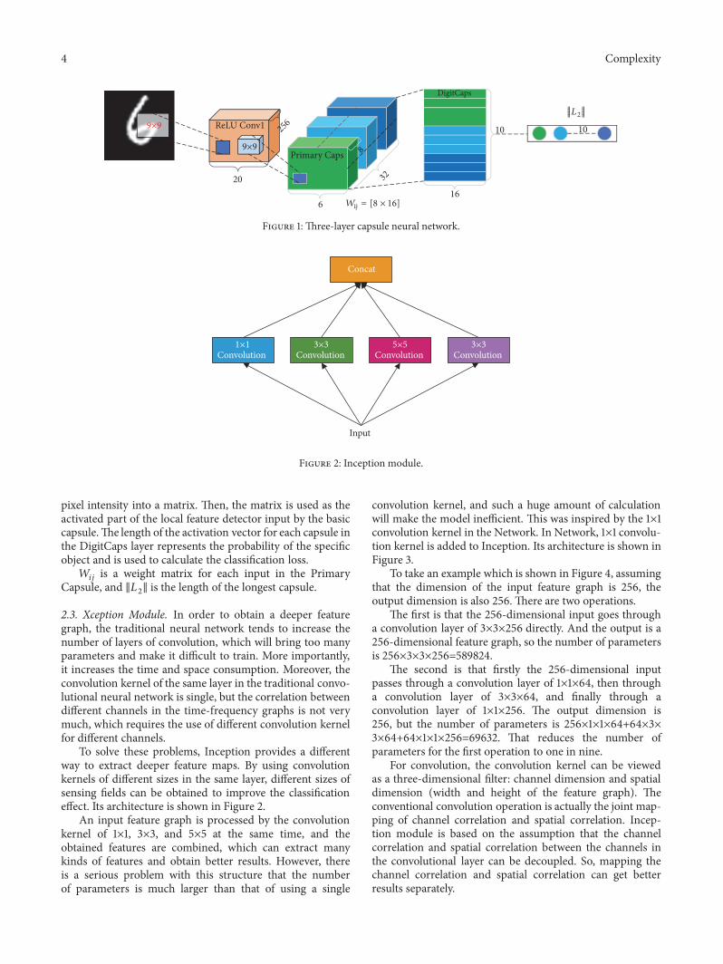
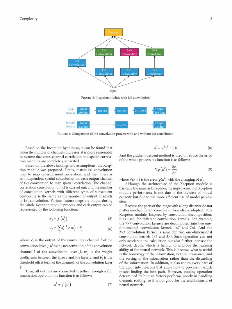
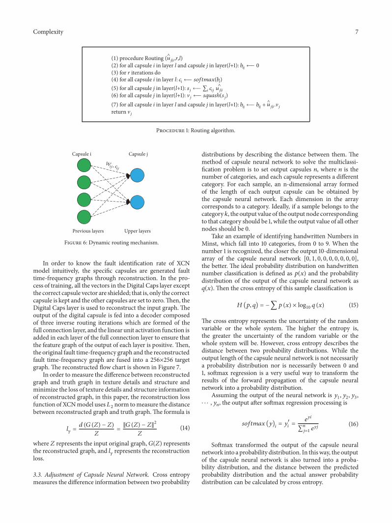
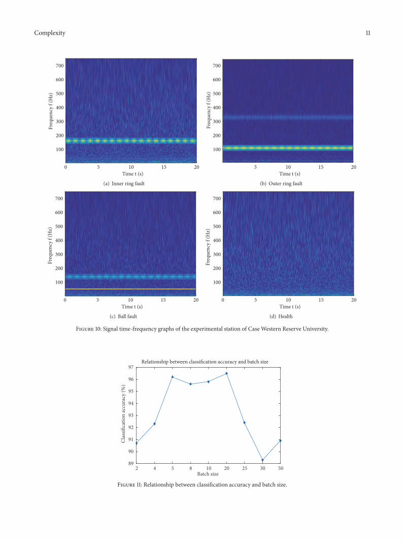
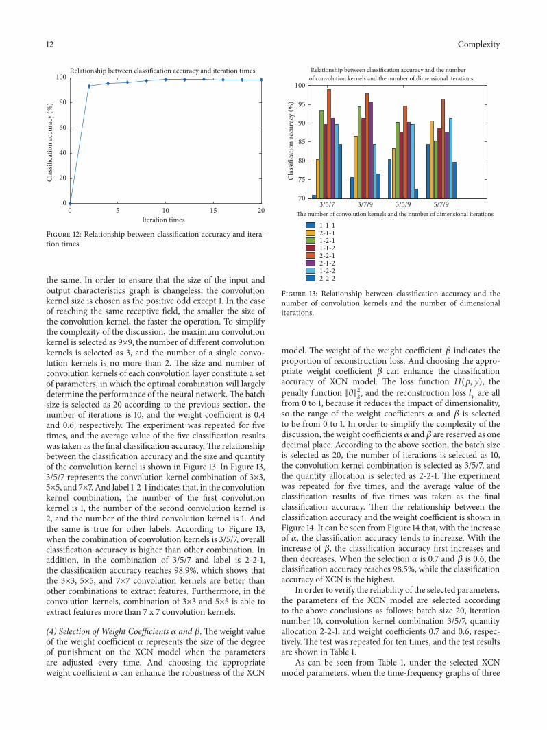
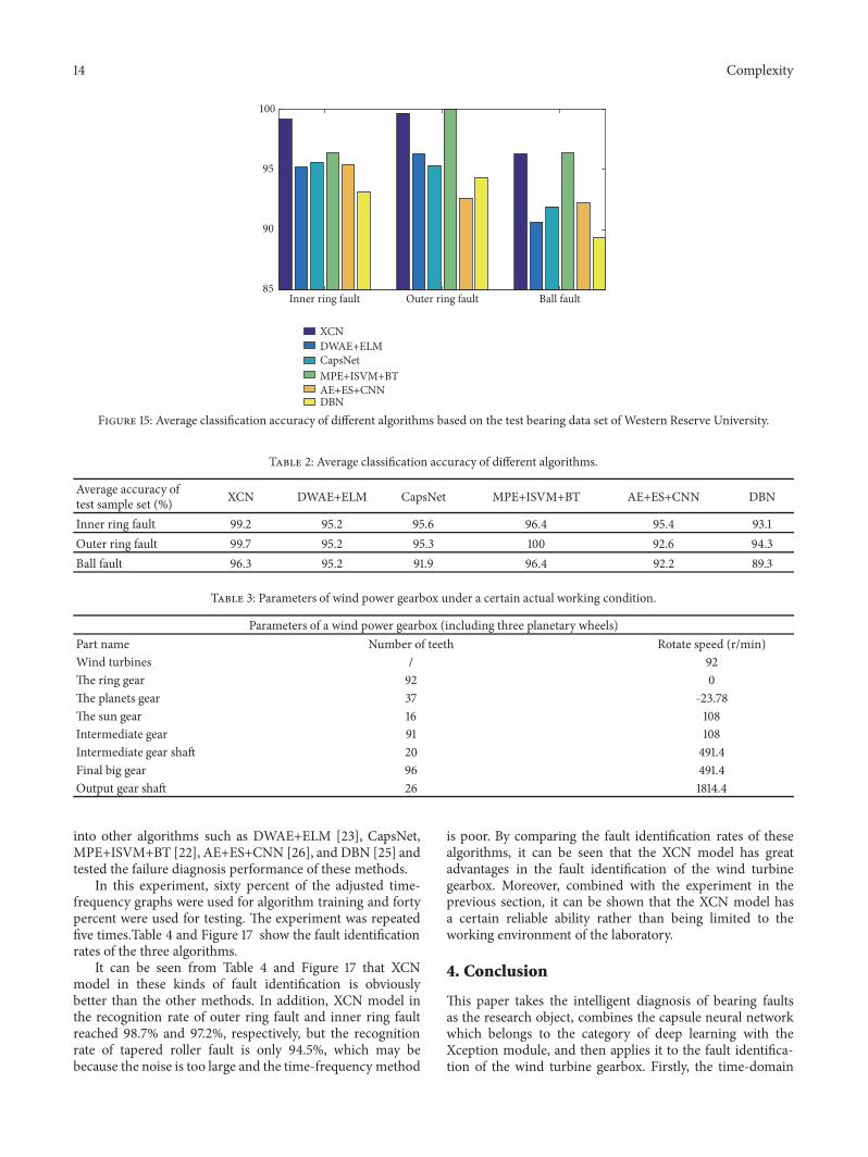
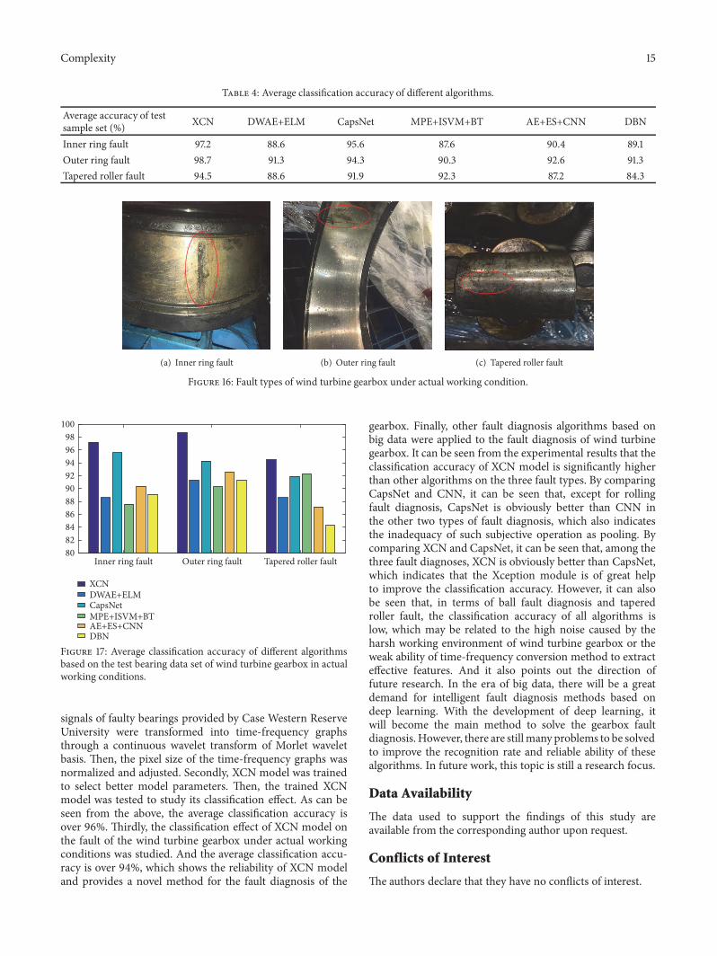

Hindawiwwwhindawicom Volume 2018
MathematicsJournal of
Hindawiwwwhindawicom Volume 2018
Mathematical Problems in Engineering
Applied MathematicsJournal of
Hindawiwwwhindawicom Volume 2018
Probability and StatisticsHindawiwwwhindawicom Volume 2018
Journal of
Hindawiwwwhindawicom Volume 2018
Mathematical PhysicsAdvances in
Complex AnalysisJournal of
Hindawiwwwhindawicom Volume 2018
OptimizationJournal of
Hindawiwwwhindawicom Volume 2018
Hindawiwwwhindawicom Volume 2018
Engineering Mathematics
International Journal of
Hindawiwwwhindawicom Volume 2018
Operations ResearchAdvances in
Journal of
Hindawiwwwhindawicom Volume 2018
Function SpacesAbstract and Applied AnalysisHindawiwwwhindawicom Volume 2018
International Journal of Mathematics and Mathematical Sciences
Hindawiwwwhindawicom Volume 2018
Hindawi Publishing Corporation httpwwwhindawicom Volume 2013Hindawiwwwhindawicom
The Scientific World Journal
Volume 2018
Hindawiwwwhindawicom Volume 2018Volume 2018
Numerical AnalysisNumerical AnalysisNumerical AnalysisNumerical AnalysisNumerical AnalysisNumerical AnalysisNumerical AnalysisNumerical AnalysisNumerical AnalysisNumerical AnalysisNumerical AnalysisNumerical AnalysisAdvances inAdvances in Discrete Dynamics in
Nature and SocietyHindawiwwwhindawicom Volume 2018
Hindawiwwwhindawicom
Dierential EquationsInternational Journal of
Volume 2018
Hindawiwwwhindawicom Volume 2018
Decision SciencesAdvances in
Hindawiwwwhindawicom Volume 2018
AnalysisInternational Journal of
Hindawiwwwhindawicom Volume 2018
Stochastic AnalysisInternational Journal of
Submit your manuscripts atwwwhindawicom