a novel rc-fdtd algorithm for the drude dispersion analysis

Progress In Electromagnetics Research M, Vol. 24, 251–264, 2012

A NOVEL RC-FDTD ALGORITHM FOR THE DRUDEDISPERSION ANALYSIS

A. Cala’ Lesina*, A. Vaccari, and A. Bozzoli

Renewable Energies and Environmental Technologies (REET), Fon-dazione Bruno Kessler (FBK-irst), I-38123 Trento, Italy

Abstract—One of the main techniques for the Finite-DifferenceTime-Domain (FDTD) analysis of dispersive media is the RecursiveConvolution (RC) method. The idea here proposed for calculating theupdating FDTD equation is based on the Laplace transform and isapplied to the Drude dispersion case. A novel RC-FDTD algorithm,that we call modified, is then deduced. We test our algorithm bysimulating gold and silver nanospheres exposed to an optical planewave and by comparing the results with the analytical solution. Themodified algorithm guarantees a better overall accuracy of the solution,in particular at the plasmonic resonance frequencies.

1. INTRODUCTION

We focus here on the explicit Finite-Difference Time-Domain (FDTD)numerical solution method of the Maxwell’s equations [1, 2], with theConvolutional Perfectly Matched Layer (CPML) boundary conditionsformulation [3]. Although some other approaches for the simulation ofDrude dispersive media already exist [4–16], we consider the RecursiveConvolution (RC) algorithm [17], that we call standard, as reference.It time-discretizes directly the convolution integral expressing thetemporal non-locality between the D and E fields. In order to minimizethe truncation error, we propose here to find a closed form solutionof the Ampere-Maxwell equation, and only after to proceed with thetime discretization. We calculate explicitly the kernel of such a closedform solution in the case of Drude media deducing the modified RCalgorithm, and show how it can be updated recursively with the samememory requirements than the standard RC scheme. The evaluation ofsome error parameters and the comparison of the electromagnetic fields

Received 19 April 2012, Accepted 23 May 2012, Scheduled 7 June 2012* Corresponding author: Antonino Cala’ Lesina ([email protected]).

252 Cala’ Lesina, Vaccari, and Bozzoli

highlight the better accuracy of the proposed modified RC algorithmwith respect to the standard one. The test has been done for Auand Ag noble metals [18] nanospheres, in the optical frequency range,and makes the modified RC algorithm suitable for the simulationof plasmonic resonant nanostructures and optical antennas, as forexample proposed in [19, 20].

2. THEORETICAL APPROACH

The temporal non-locality relation between the D and E fields indispersive media is expressed by means of the convolution integral

D(t) = ε0ε∞E(t) + ε0

∫ t

0E(t− τ)χ(τ)dτ (1)

which exhibits a Dirac-delta contribution representing the instanta-neous response at the infinite frequency through the (relative) permit-tivity ε∞ term. In (1) χ (τ) is the inverse Fourier transform of theelectric susceptibility χ (ω). This measures the media polarization andenters the complex permittivity ε (ω) in

D(ω) = ε0 [ε∞ + χ(ω)]E(ω) = ε(ω)E(ω), (2)i.e., the proportionality coefficient between D and E in the angularfrequency domain ω after a Fourier transform with respect to the timevariable. In (2) the same letters are used to denote the fields both in thetime and frequency domain and the space dependence is understood.The Ampere-Maxwell equation which is time stepped in the FDTDmethod, along with the Faraday-Maxwell curl equation for the E andB fields, is

∇×H =∂D∂t

+ σE, (3)

where σ is the static conductivity contribution. Before discretizing (3)for time stepping however, we analytically solve it with respect to thetime variable by the Laplace transform method, to get a closed formsolution for the electric field E at a given time instant t. If we denote bys the dual of the time variable t, omit an understood space dependenceas before, and now use a tilde for a Laplace transformed quantity, wehave from (1)

D(s) = ε0 [ε∞ + χ(s)] E(s) (4)

and from (3)

∇× H(s) = sD(s)−D(0) + σE(s), (5)where we assumed that the curl operator ∇×, acting on the spacevariables, commutes with the Laplace transform operator. By solving

Progress In Electromagnetics Research M, Vol. 24, 2012 253

for D (s) the first of the two previous equations, inserting the resultin the second one, where an initial time zero-field condition has beenassumed, and then solving for E (s) we have

E(s) = G(s) ·∇× H(s), (6)

where G (s) stands for

G(s) =1

sε0 [ε∞ + χ(s)] + σ. (7)

Note that χ(s = −iω) = χ(ω) where i =√−1 is the imaginary unit.

By returning to the time domain through an inverse Laplace transform,we get the aforementioned closed form exact solution for the electricfield

E(t) =∫ t

0G(t− τ) ·∇×H(τ)dτ, (8)

where the convolutional kernel G (τ) depends on the medium dispersioncharacteristic. Note that if in (1) χ (τ) were identically zero, we wouldrecover the usual non-dispersive behavior with the absolute dielectricconstant ε = ε0ε∞. This would imply an identically zero χ in (7) too.For the corresponding original G we would then get

G(τ) =1εe−

σετ , (9)

where a Heaviside step function factor of argument is understood.Using this result in (8) and, as is usual in FDTD, sampling at discretetimes nδt, where δt is the time-step, with ∇ ×H and H temporallysampled halfway at (n + 1/2)δt, one gets an updating equation for Ewith exponential coefficients

En+1 = e−σδtε En +

(1− e−

σδtε

)

σ∇×Hn+ 1

2 , (10)

where superscripts denote time levels. By Taylor expanding to firstorder the coefficients in (10) with respect to the small quantity σδt/ε,they equal their FDTD discrete counterparts expanded to the sameorder. With this in mind we think that our approach based on (8)is less prone to time truncation errors, mainly for highly absorptivemedia with rapidly time decaying fields, than the standard methodbased on an early discretization of the convolution integral (1).

We now calculate explicitly the convolutional kernel G (s) shownin (7) in the case of Drude dispersion. This is formulated by the singleterm electric susceptibility

χ(s) =ω2

D

s(s + γ), (11)


where ωD and γ are the plasma frequency and the damping coefficient.This gives

G(s) =s + γ

ε0ε∞(s− s+)(s− s−), (12)

wheres± = −P ± iQ (13)

and

P =12

(γ +

σ

ε0ε∞

), Q =

√ε0ω2

D + σγ

ε0ε∞− P 2 . (14)

After returning to the time-domain we get

G(τ) =1

ε0ε∞

[es+τ (s+ + γ)

s+ − s−+

es−τ (s− + γ)s− − s+

](15)

which, putting

S =12

(γ − σ

ε0ε∞

), (16)

has the following form

G(τ) = ={

Ke−Wτ+iΦ}

, (17)

where

K =1

ε0ε∞

√1 +

(S

Q

)2

, (18)

W = P − iQ, (19)

Φ = arctanQ

S, (20)

with K and Φ real quantities. < and = denote the real and imaginaryparts of a complex quantity. By defining the complex vector

Ψ(t) =∫ t

0Ke−W (t−τ)+iΦ ·∇×H(τ)dτ (21)

one sees that, according with (8) and (17), the electric field E resultsto be

E(t) = ={Ψ(t)} =∫ t

0=

{Ke−W (t−τ)+iΦ

}·∇×H(τ)dτ. (22)

Sampling (21) at the discrete times nδt (n = 1, 2, . . .) we have

Ψn+1 =∫ (n+1)δt

0Ke−W ((n+1)δt−τ)+iΦ ·∇×H(τ)dτ. (23)


Separating the integration interval we obtain

Ψn+1 = e−Wδt

∫ nδt

0Ke−W (nδt−τ)+iΦ ·∇×H(τ)dτ

+∇×Hn+ 12 ·

∫ (n+1)δt

nδtKe−W ((n+1)δt−τ)+iΦdτ (24)

and thenΨn+1 = e−Wδt ·Ψn + A ·∇×Hn+ 1

2 , (25)

where the complex coefficient A is given by

A =∫ (n+1)δt

nδtKe−W ((n+1)δt−τ)+iΦdτ = K

eiΦ(1− e−Wδt

)

W. (26)

Thus storing, as in the RC traditional scheme [17], one extra complexvariable for each sampling point and each electric field component,updating it according to (25), and using its imaginary part as a newelectric field value, allows us to include dispersive media in a simplerand more accurate recursive procedure. By expanding the exponentialfactor according to the Euler formula

e−Wδt = e−Pδt · [cos(Qδt) + i sin(Qδt)] (27)

and taking the imaginary part of both sides of (25) we have themodified form of the electric field updating equation

En+1 = e−Pδt sin(Qδt) · < {Ψn}+e−Pδt cos(Qδt) ·En + ={A} ·∇×Hn+ 1

2 . (28)

For completeness we report the updating equation of the standardmethod [17]:

En+1 = C1 ·Φn + C2 ·En + C3 ·∇×Hn+ 12 , (29)

whereΦn = C4 ·En−1 + e−γδt ·Φn−1 (30)

and

C1 =1

ε0 + χ0, (31)

C2 = (ε∞ + ∆χ0)C1, (32)

C3 =δt

ε0C1, (33)

C4 = e−γδt∆χ0, (34)

χ0 =∫ δt

0χ(τ)dτ, (35)


∆χ0 = −ω2D

γ

[1− e−γδt

]2. (36)

3. SIMULATIONS

To test the modified RC algorithm previously proposed, we apply it toa 96 nm radius nanosphere, made of gold or silver, in a monochromaticlight beam. The static conductivity is assumed null. We have testedour modified algorithm in particular for Au at λ = 480 nm and for Ag atλ = 336 nm and λ = 380 nm, i.e., the resonance wavelengths evidencedin Fig. 1 through the extinction coefficient Cext defined in [21]. Thiscoefficient is an efficiency parameter defined as the ratio of the particlecross section over a surface which is the geometrical projection of theparticle on a plane perpendicular to the incoming field. The extinction,scattering and absorption coefficients for a spherical particle are:

Cext =2

r2k2

∞∑

m=1

(2m + 1)<(am + bm), (37)

Csca =2

r2k2

∞∑

m=1

(2m + 1)(|am|2 + |bm|2

), (38)

Figure 1. Analytical Cext for Au and Ag nanospheres (r = 96 nm)modeled by Drude dispersion.


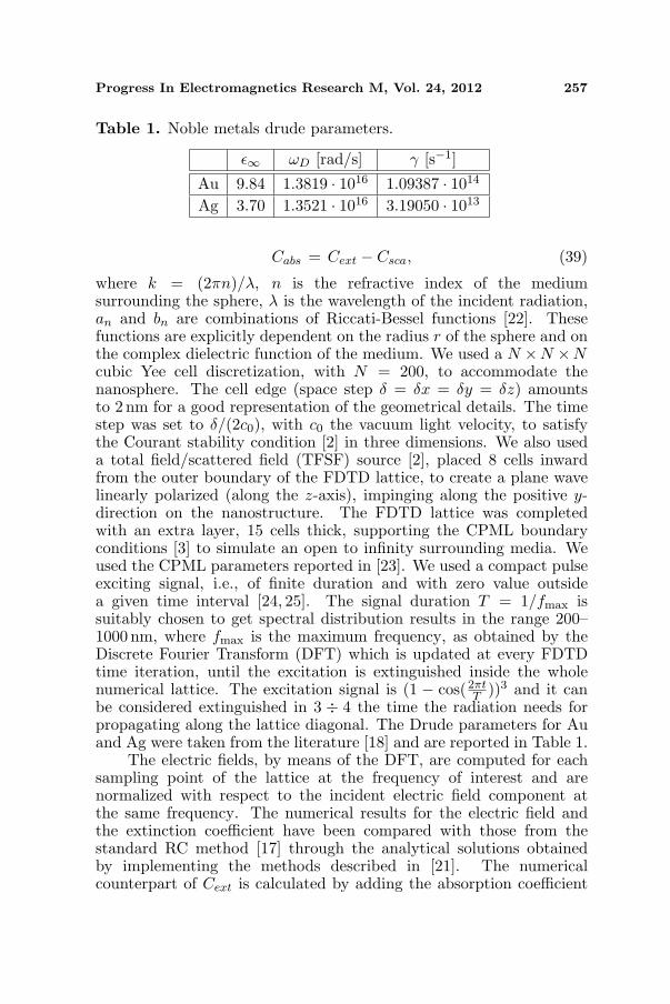
Table 1. Noble metals drude parameters.

ε∞ ωD [rad/s] γ [s−1]

Au 9.84 1.3819 · 1016 1.09387 · 1014

Ag 3.70 1.3521 · 1016 3.19050 · 1013

Cabs = Cext − Csca, (39)

where k = (2πn)/λ, n is the refractive index of the mediumsurrounding the sphere, λ is the wavelength of the incident radiation,an and bn are combinations of Riccati-Bessel functions [22]. Thesefunctions are explicitly dependent on the radius r of the sphere and onthe complex dielectric function of the medium. We used a N ×N ×Ncubic Yee cell discretization, with N = 200, to accommodate thenanosphere. The cell edge (space step δ = δx = δy = δz) amountsto 2 nm for a good representation of the geometrical details. The timestep was set to δ/(2c0), with c0 the vacuum light velocity, to satisfythe Courant stability condition [2] in three dimensions. We also useda total field/scattered field (TFSF) source [2], placed 8 cells inwardfrom the outer boundary of the FDTD lattice, to create a plane wavelinearly polarized (along the z-axis), impinging along the positive y-direction on the nanostructure. The FDTD lattice was completedwith an extra layer, 15 cells thick, supporting the CPML boundaryconditions [3] to simulate an open to infinity surrounding media. Weused the CPML parameters reported in [23]. We used a compact pulseexciting signal, i.e., of finite duration and with zero value outsidea given time interval [24, 25]. The signal duration T = 1/fmax issuitably chosen to get spectral distribution results in the range 200–1000 nm, where fmax is the maximum frequency, as obtained by theDiscrete Fourier Transform (DFT) which is updated at every FDTDtime iteration, until the excitation is extinguished inside the wholenumerical lattice. The excitation signal is (1 − cos(2πt

T ))3 and it canbe considered extinguished in 3 ÷ 4 the time the radiation needs forpropagating along the lattice diagonal. The Drude parameters for Auand Ag were taken from the literature [18] and are reported in Table 1.

The electric fields, by means of the DFT, are computed for eachsampling point of the lattice at the frequency of interest and arenormalized with respect to the incident electric field component atthe same frequency. The numerical results for the electric field andthe extinction coefficient have been compared with those from thestandard RC method [17] through the analytical solutions obtainedby implementing the methods described in [21]. The numericalcounterpart of Cext is calculated by adding the absorption coefficient


Figure 2. Error parameters Lξ,η and Lξ comparison for Au (DFT atλ = 480 nm).

Table 2. Error evaluation at the resonance frequencies.

Au (480 nm) Ag (336 nm) Ag (380 nm)

Lm,x (Ls,x) 0.0386 (0.0548) 0.1275 (0.1533) 0.0374 (0.0421)Lm,y (Ls,y) 0.0592 (0.0872) 0.2085 (0.2485) 0.0585 (0.0687)Lm,z (Ls,z) 0.0440 (0.0633) 0.1718 (0.2024) 0.0430 (0.0478)Lm (Ls) 0.0693 (0.1011) 0.2670 (0.3282) 0.0594 (0.0684)

LCm (LCs) 0.2216 (0.3376) 0.3265 (0.3646) 0.4579 (0.5052)

Cabs to the scattering coefficient Csca, indeed only these two areevaluable through a numerical approach. The first is the Poyntingvector flux through a closed surface containing the sphere in thetotal field domain, the second is calculated by means of the sameflux through a closed surface located in the scattered field region.In order to evaluate the deviation of the numerical results from theexact solution we considered the average error for each electric fieldcomponent

Lξ,η =1

N3

N∑

i,j,k=1

∣∣∣Eξη(i, j, k)− Ea

η (i, j, k)∣∣∣ , (40)


Table 3. LCξ over the total frequency range.

Au Ag

LCm (LCs) 0.0515 (0.0747) 0.0926 (0.1019)

Figure 3. Total field Ex, Ey, Ez for Au nanosphere (DFT atλ = 480 nm) along the x axis (y = 170, z = 120).

the average error for the electric field module

Lξ =1

N3

N∑

i,j,k=1

∣∣∣∣∣∣Eξ(i, j, k)

∣∣∣−∣∣∣Ea(i, j, k)

∣∣∣∣∣∣ (41)

and the average error for Cext

LCξ =1

Nλ

Nλ∑

i=1

∣∣∣Cξexti

− Caexti

∣∣∣ , (42)

where η = {x, y, z} indicates the cartesian component, ξ = {s, m}, theletters s, m, a denote standard, modified and analytical solution, andNλ is the number of wavelengths at which Cext has been evaluated. Thevalues in Table 2 were obtained with 12000 time iterations simulations.For the gold resonance the error parameters (40) and (41) are reportedas a function of the number of FDTD iterations (Fig. 2). We canobserve that the convergence is reached after the same number ofFDTD time iterations than in the standard case and in all the cases


Figure 4. Total field Ex, Ey, Ez for Au nanosphere (DFT atλ = 480 nm) along the y axis (x = 150, z = 150).

Figure 5. Total field Ex, Ey, Ez for Au nanosphere (DFT atλ = 480 nm) along the z axis (x = 150, y = 170).


Wavelength [nm]

Cext

0

1

2

3

4

5

6

7

8

200 300 400 500 600 700 800

Figure 6. Cext for a gold nanosphere (r = 96 nm) modeled by Drudedispersion.

Figure 7. LCξ comparison for gold in the total frequency range, andin the region of Cext minimum and maximum.


the level of accuracy is better. The better numerical accuracy is alsoevidenced with a comparison of the total electric field extracted fromthe lattice along one direction in x, y and z (Figs. 3–5). In each figurethe three components of the electric field (Ex on the left, Ey in themiddle and Ez on the right) are represented. The sharp peaks are dueto the field inside the sphere, that is very low (metallic sphere), and tosome symmetry planes where the field is zero. For gold and silver theextinction coefficient has been calculated and the error parameter (42)at the resonance frequencies (Table 2) and over the total frequencyrange are reported (Table 3). For gold moreover the Cext comparisonis shown in Fig. 6, while in Fig. 7 the error parameter (42) is evaluatedfor the total frequency range and in the peak regions (λ = 400 nm andλ = 480 nm) varying the number of time iterations.

4. CONCLUSION

We proposed a modified Recursive Convolution algorithm for theFDTD analysis of Drude dispersive media. The algorithm has beentested by comparing the electric field and the extinction coefficientdeviation from the analytical solution for gold and silver nanospheres.It evidences an accuracy improvement with respect to the standardRC method. The better precision is observable in particular at theplasmonic resonance frequencies and makes the modified algorithmsuitable for plasmonic simulations.

REFERENCES

1. Yee, K. S., “Numerical solution of initial boundary value problemsinvolving Maxwell’s equations in isotropic media,” IEEE Trans. onAntennas and Propagat., Vol. 14, No. 3, 302–307, 1966.

2. Taflove, A. and S. C. Hagness, Computational Electrodynamics:The Finite-difference Time-domain Method, 3rd Edition, ArtechHouse, Norwood, MA, 2005.

3. Roden, J. A. and S. D. Gedney, “Convolution PML (CPML):An efficient FDTF implementation of the CFS-PML for arbitrarymedia,” Microwave and Optical Technology Letters, Vol. 27, No. 5,334–339, 2000.

4. Sullivan, D. M., “Frequency-dependent FDTD methods using Ztransforms,” IEEE Trans. on Antennas and Propagat., Vol. 40,1223–1230, 1992.

5. Gandhi, O. P., B.-H. Gao, and J.-Y. Chen, “A frequency-dependent finite-difference time-domain formulation for general


dispersive media,” IEEE Trans. on Microwave Theory and Tech.,Vol. 41, 658–665, 1993.

6. Young, J. L., “Propagation in linear dispersive media: Finitedifference time-domain methodologies,” IEEE Trans. on Antennasand Propagat., Vol. 43, 422–426, 1995.

7. Pereda, J. A., L. A. Vielva, A. Vegas, and A. Prieto, “Statespaceapproach to the FDTD formulation for dispersive media,” IEEETrans. on Magn., Vol. 31, 1602–1605, 1995.

8. Kelly, D. F. and R. J. Luebbers, “Piecewise linear recursiveconvolution for dispersive media using FDTD,” IEEE Trans. onAntennas and Propagat., Vol. 44, 792–797, 1996.

9. Okoniewski, M., M. Mrozowski, and M. A. Stuchly, “Simpletreatment of multi-term dispersion in FDTD,” IEEE MicrowaveGuided Wave Lett., Vol. 7, 121–123, 1997.

10. Chen, Q., M. Katsuari, and P. H. Aoyagi, “An FDTD formulationfor dispersive media using a current density,” IEEE Trans. onAntennas and Propagat., Vol. 46, 1739–1746, 1998.

11. Pereda, J. A., A. Vegas, and A. Prieto, “FDTD modelingof wave propagation in dispersive media by using the Mobiustransformation technique,” IEEE Trans. on Microwave Theoryand Tech., Vol. 50, 1689–1695, 2002.

12. Okoniewski, M. and E. Okoniewska, “Drude dispersion in ADEFDTD revisited,” Electronics Letters, Vol. 42, No. 9, 503–504,2006.

13. Kong, S., J. J. Simpson, and V. Backman, “ADE-FDTDscattered-field formulation for dispersive materials,” IEEEMicrowave and Wireless Components Lett., Vol. 18, No. 1, 4–6,Jan. 1, 2008.

14. Shibayama, J., et al., “Simple trapezoidal recursive convolutiontechnique for the frequency-dependent FDTD analysis of a drude-lorentz model,” IEEE Photonics Technology Letters, Vol. 21,No. 2, 100–102, Jan. 15, 2009.

15. Alsunaidi, M. A. and A. A. Al-Jabr, “A general ADE-FDTD algorithm for the simulation of dispersive structures,”IEEE Photonics Technology Letters, Vol. 21, No. 12, 817–819,Jun. 15, 2009.

16. Zhang, Y.-Q. and D.-B. Ge, “A unified FDTD approachfor electromagnetic analysis of dispersive objects,” Progress InElectromagnetics Research, Vol. 96, 155–172, 2009.

17. Luebbers, R. J., F. Hunsberger, and K.S. Kunz, “A frequency-dependent finite-difference time-domain formulation for transient


propagation in plasma,” IEEE Trans. on Antennas and Propagat.,Vol. 39, No. 1, 29–34, 1991.

18. Kolwas, K., A. Derkachova, and M. Shopa, “Size characteristics ofsurface plasmons and their manifestation in scattering propertiesof metal particles,” Journal of Quantitative Spectroscopy &Radiative Transfer, Vol. 110, 1490–1501, 2009.

19. Lee, K. H., I. Ahmed, R. S. M. Goh, E. H. Khoo, E. P. Li,and T. G. G. Hung, “Implementation of the FDTD methodbased on Lorentz-Drude dispersive model on GPU for plasmonicsapplication,” Progress In Electromagnetics Research, Vol. 116,441–456, 2011.

20. Paris, A., A. Vaccari, A. Cala’ Lesina, E. Serra, and L. Calliari,“Plasmonic scattering by metal nanoparticles for solar cells,”Plasmonics, 1–10, March 8, 2012.

21. Stratton, J. A., Electromagnetic Theory, McGraw-Hill, New Yorkand London, 1941.

22. Bohren, C. F. and D. R. Huffman, Absorption and Scattering ofLight by Small Particles, Wiley, New York, 1998.

23. Laakso, I., S. Ilvonen, and T. Uusitupa, “Performance ofconvolutional PML absorbing boundary conditions in finite-difference time-domain SAR calculations,” Phys. Med. Biol.,Vol. 52, 7183–7192, 2007.

24. Pontalti, R., L. Cristoforetti, and L. Cescatti, “The frequency de-pendent FD-TD method for multi-frequency results in microwavehyperthermia treatment simulation,” Phys. Med. Biol., Vol. 38,1283–1298, 1993.

25. Vaccari, A., R. Pontalti, C. Malacarne, and L. Cristoforetti,“A robust and efficient subgridding algorithm for finite-differencetime-domain simulations of Maxwell’s equations,” J. Comput.Phys., Vol. 194, 117–139, 2003.

a novel rc-fdtd algorithm for the drude dispersion analysis

Documents