March 2004

NASA/CR-2004-212669

A Novel, Real-Valued Genetic Algorithm forOptimizing Radar Absorbing Materials

John Michael HallLockheed Martin Space Operations, Hampton, Virginia

The NASA STI Program Office . . . in Profile

Since its founding, NASA has been dedicated to theadvancement of aeronautics and space science. TheNASA Scientific and Technical Information (STI)Program Office plays a key part in helping NASAmaintain this important role.

The NASA STI Program Office is operated byLangley Research Center, the lead center for NASA’sscientific and technical information. The NASA STIProgram Office provides access to the NASA STIDatabase, the largest collection of aeronautical andspace science STI in the world. The Program Office isalso NASA’s institutional mechanism fordisseminating the results of its research anddevelopment activities. These results are published byNASA in the NASA STI Report Series, whichincludes the following report types:

• TECHNICAL PUBLICATION. Reports of

completed research or a major significant phaseof research that present the results of NASAprograms and include extensive data ortheoretical analysis. Includes compilations ofsignificant scientific and technical data andinformation deemed to be of continuingreference value. NASA counterpart of peer-reviewed formal professional papers, but havingless stringent limitations on manuscript lengthand extent of graphic presentations.

• TECHNICAL MEMORANDUM. Scientific

and technical findings that are preliminary or ofspecialized interest, e.g., quick release reports,working papers, and bibliographies that containminimal annotation. Does not contain extensiveanalysis.

• CONTRACTOR REPORT. Scientific and

technical findings by NASA-sponsoredcontractors and grantees.

• CONFERENCE PUBLICATION. Collected

papers from scientific and technicalconferences, symposia, seminars, or othermeetings sponsored or co-sponsored by NASA.

• SPECIAL PUBLICATION. Scientific,

technical, or historical information from NASAprograms, projects, and missions, oftenconcerned with subjects having substantialpublic interest.

• TECHNICAL TRANSLATION. English-

language translations of foreign scientific andtechnical material pertinent to NASA’s mission.

Specialized services that complement the STIProgram Office’s diverse offerings include creatingcustom thesauri, building customized databases,organizing and publishing research results ... evenproviding videos.

For more information about the NASA STI ProgramOffice, see the following:

• Access the NASA STI Program Home Page athttp://www.sti.nasa.gov

• E-mail your question via the Internet to

help@sti.nasa.gov • Fax your question to the NASA STI Help Desk

at (301) 621-0134 • Phone the NASA STI Help Desk at

(301) 621-0390 • Write to:

NASA STI Help Desk NASA Center for AeroSpace Information 7121 Standard Drive Hanover, MD 21076-1320

National Aeronautics andSpace Administration

Langley Research Center Prepared for Langley Research CenterHampton, Virginia 23681-2199 under Contract NAS1-00135

March 2004

NASA/CR-2004-212669

A Novel, Real-Valued Genetic Algorithm forOptimizing Radar Absorbing Materials

John Michael HallLockheed Martin Space Operations, Hampton, Virginia

Available from:

NASA Center for AeroSpace Information (CASI) National Technical Information Service (NTIS)7121 Standard Drive 5285 Port Royal RoadHanover, MD 21076-1320 Springfield, VA 22161-2171(301) 621-0390 (703) 605-6000

- 1 -

Contents

Abstract 2

I. Introduction 3 II. The Problem 4 III. The Chromosomal Representation 5 IV. The Genesis Population 7 V. Pseudo-Random Number Generation 8 VI. Determining Fitness by Mode Matching 8 VII. Survival of the Most Diverse 12 VIII. Total Score and Extinction 13 IX. Propagation of the Species 15 X. Hybridization 18 XI. Mutation 18 XII. Results – Fictitious absorbers 22 XIII. Results – Real absorbers 25 XIV. Conclusion 28 XV. Acknowledgments 28 XVI. References 29 XVII. Appendix – Flowchart 30

- 2 -

Abstract

A novel, real-valued Genetic Algorithm (GA) was designed and implemented to

minimize the reflectivity and/or transmissivity of an arbitrary number of homogeneous, lossy

dielectric or magnetic layers of arbitrary thickness positioned at either the center of an infinitely

long rectangular waveguide, or adjacent to the perfectly conducting backplate of a semi-infinite,

shorted-out rectangular waveguide. Input is specified as the number of layers, their locations and

thicknesses, the frequency band of interest, and the upper and lower bounds on the physioelectric

constants to be obtained. Scattering is then minimized over the frequency band of interest using

optimization strategies based upon principles of Artificial Intelligence (AI). Evolutionary

processes extract the optimal physioelectric constants falling within specified constraints which

minimize reflection and/or transmission over the frequency band of interest. Output in the form

of the physiolectric constants of the layers and the scattering parameters of the entire stack is

provided. This GA extracted the unphysical dielectric and magnetic constants of three layers of

fictitious material placed adjacent to the conducting backplate of a shorted-out waveguide such

that the reflectivity of the configuration was –55 dB or less over the entire X-band. This numeric

Absorbing Boundary Condition (ABC) was validated by showing that the reflectivity of test

cases backed with the ABC was identical to the reflectivity of those test cases backed by free

space, to within 0.23% relative difference. This ABC could be used to numerically truncate

open-region boundaries in Finite Element (FEM) waveguide problems, thereby eliminating the

need to use the Method of Moments (MoM). Although this GA was specifically designed for

creating “fictitious absorber” type ABCs to truncate FEM meshes, it can also be used to design

real Radar Absorbing Materials (RAM). Examples of the optimization of realistic multi-layer

absorbers will also be reported. Although typical Genetic Algorithms require populations of

many thousands in order to function properly and obtain correct results, verified correct results

were obtained for all test cases using this GA with a population of only four.

- 3 -

I. Introduction - Artificial Intelligence (AI) is the study of computations which make it possible to

perceive, reason, and act. Although the scientific goal of AI is to understand various sorts of

natural intelligence, the engineering goal is to solve real-world problems. Since the inception of

automated computation, conventional wisdom has held that computers can only do what they are

told to do, and nothing more. However, contemporary applications of AI demonstrate that under

certain circumstances, computers can acquire the ability to solve ambiguous problems which

programmers generally have no clue how to solve, through the modeling of biological cognition

and natural selection processes. The application of AI to real-world problems provides an

ingenious avenue for technological advancement, which through its application sheds new light

on questions traditionally asked by psychologists, linguists, and philosophers. The answers to

these questions may help us become more intelligent, ourselves.

In his magnum opus, “The Origin of the Species” [1], Charles Darwin described the

principle of evolution through natural selection, which after much heated debate, became

generally accepted among scientists. Darwin’s principle states that:

¾�Each individual tends to pass on its traits to its offspring.

¾�Nevertheless, nature produces individuals with differing traits.

¾�The fittest individuals – those with more favorable traits – tend to have more

offspring than do those with unfavorable traits, thus driving the population as a whole

toward favorable traits.

¾�Over long periods, variation can accumulate, producing entirely new species whose

traits make them especially suited to particular ecological niches.

From a molecular-biological standpoint, Darwin’s natural selection is enabled by

variation in the species arising from mutation, which produces new genes previously unseen in

the population, and crossover, which is the random recombination of genetic material that occurs

during reproduction.

According to Darwin, successful evolutionary processes are neither purposeful nor

directed. They require no foreknowledge of their final destination in order to eventually get

there. For example, there is no scientific evidence to support the assertion that the purpose of

evolution in nature is to produce Humankind. Instead, the success of the process seems to boil

- 4 -

down to a handful of simple principles operating in the context of individuals competing for

resources in their environment. This unique capacity for improvement without foreknowledge of

the eventual result offers a powerful way to solve ambiguous problems which may be otherwise

insoluble using canonical formalism.

The Genetic Algorithm (GA), first introduced by John Holland in 1975 [2], is a model

of machine learning which derives its behavior from a metaphor of evolution in Nature. Genetic

Algorithms are used for a number of different applications, including multidimensional

optimization problems where each chromosome in the population is a vector of numeric values

which encodes the different parameters being optimized. The machine creates an initially

random population of individuals represented by these chromosomes, and then subjects those

individuals to selection pressure within an evolutionary simulation.

A GA is generally implemented using the following basic cycle of operations [3]:

¾� Evaluate the fitness of all individuals within the population.

¾� Individuals not meeting or exceeding the extinction criterion die; only the fittest

survive. The empty spaces leave room for progeny.

¾� Create new progeny to replace extinguished individuals through fitness-proportionate

reproduction (and subsequent genetic recombination) of the survivors.

¾� Account for the possibility of mutation (i.e., random environmental perturbations of

chromosomal values) in the progeny who were just created.

¾� Repeat using the new population. Each iteration is known as a generation.

A more detailed flowchart illustrating the sequence of operations implemented in this GA

is provided in the Appendix to this report, with each step explained sequentially in the text.

Although simplistic from a biologist’s viewpoint, these algorithms are sufficiently complex to

provide robust and powerful mechanisms for adaptive search.

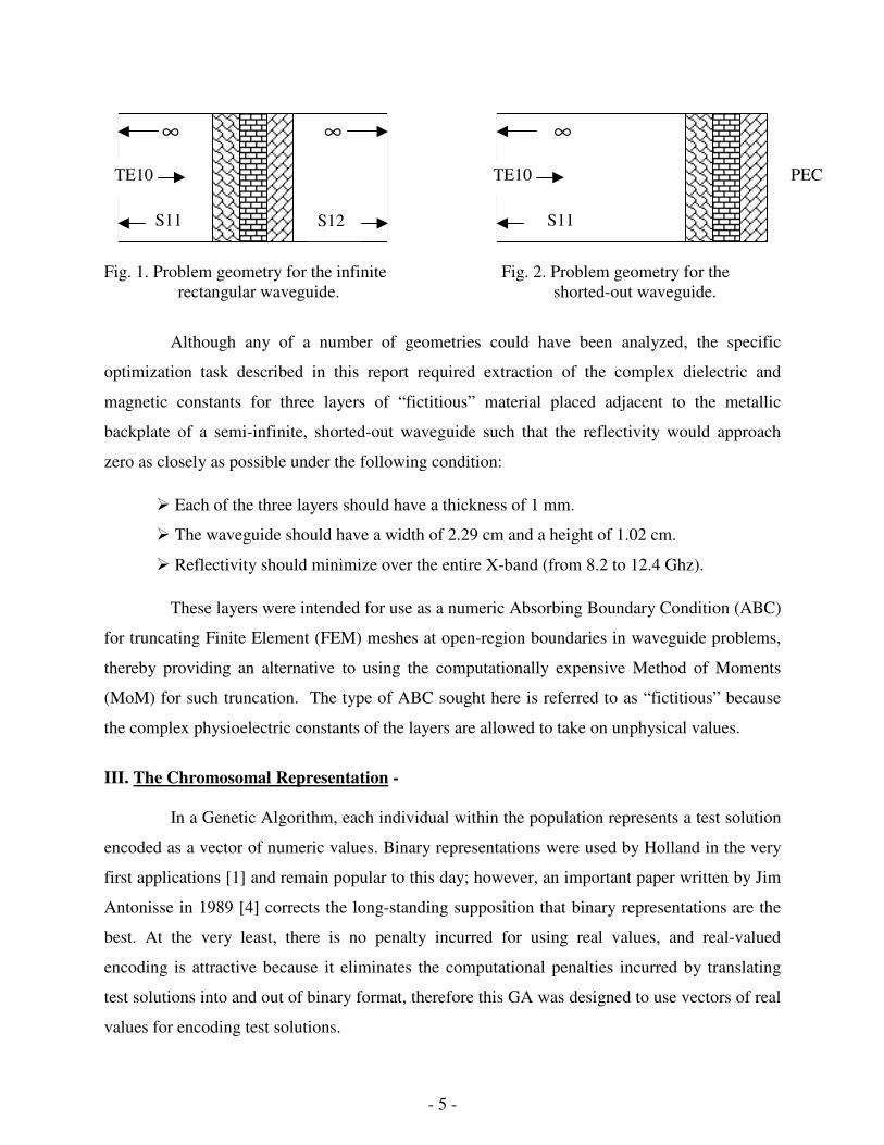
II. The Problem - Consider a finite number of lossy magnetic and/or dielectric layers stacked at the center

of an infinite rectangular waveguide, as shown in Fig. 1, or stacked against the metallic backplate

of a shorted-out, semi-infinite waveguide, as shown in Fig. 2. Each layer is homogeneous, and

will be characterized by its thickness, location, complex relative dielectric permittivity

’ ’’r jε ε ε= − ⋅ , and complex relative magnetic permeability ’ ’’r jµ µ µ= − ⋅ .

- 5 -

Fig. 1. Problem geometry for the infinite Fig. 2. Problem geometry for the rectangular waveguide. shorted-out waveguide.

Although any of a number of geometries could have been analyzed, the specific

optimization task described in this report required extraction of the complex dielectric and

magnetic constants for three layers of “fictitious” material placed adjacent to the metallic

backplate of a semi-infinite, shorted-out waveguide such that the reflectivity would approach

zero as closely as possible under the following condition:

¾� Each of the three layers should have a thickness of 1 mm.

¾� The waveguide should have a width of 2.29 cm and a height of 1.02 cm.

¾� Reflectivity should minimize over the entire X-band (from 8.2 to 12.4 Ghz).

These layers were intended for use as a numeric Absorbing Boundary Condition (ABC)

for truncating Finite Element (FEM) meshes at open-region boundaries in waveguide problems,

thereby providing an alternative to using the computationally expensive Method of Moments

(MoM) for such truncation. The type of ABC sought here is referred to as “fictitious” because

the complex physioelectric constants of the layers are allowed to take on unphysical values.

III. The Chromosomal Representation - In a Genetic Algorithm, each individual within the population represents a test solution

encoded as a vector of numeric values. Binary representations were used by Holland in the very

first applications [1] and remain popular to this day; however, an important paper written by Jim

Antonisse in 1989 [4] corrects the long-standing supposition that binary representations are the

best. At the very least, there is no penalty incurred for using real values, and real-valued

encoding is attractive because it eliminates the computational penalties incurred by translating

test solutions into and out of binary format, therefore this GA was designed to use vectors of real

values for encoding test solutions.

PEC

∞ ∞ ∞

TE10

S11

TE10

S11 S12

- 6 -

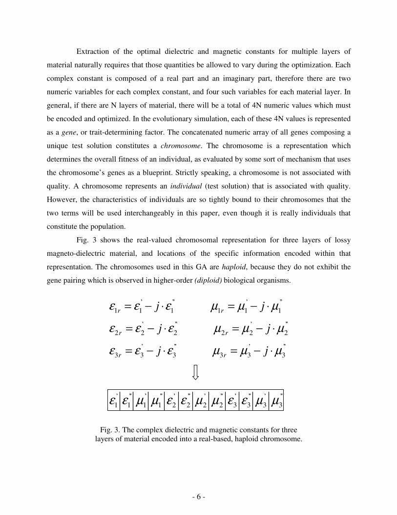
Extraction of the optimal dielectric and magnetic constants for multiple layers of

material naturally requires that those quantities be allowed to vary during the optimization. Each

complex constant is composed of a real part and an imaginary part, therefore there are two

numeric variables for each complex constant, and four such variables for each material layer. In

general, if there are N layers of material, there will be a total of 4N numeric values which must

be encoded and optimized. In the evolutionary simulation, each of these 4N values is represented

as a gene, or trait-determining factor. The concatenated numeric array of all genes composing a

unique test solution constitutes a chromosome. The chromosome is a representation which

determines the overall fitness of an individual, as evaluated by some sort of mechanism that uses

the chromosome’ s genes as a blueprint. Strictly speaking, a chromosome is not associated with

quality. A chromosome represents an individual (test solution) that is associated with quality.

However, the characteristics of individuals are so tightly bound to their chromosomes that the

two terms will be used interchangeably in this paper, even though it is really individuals that

constitute the population.

Fig. 3 shows the real-valued chromosomal representation for three layers of lossy

magneto-dielectric material, and locations of the specific information encoded within that

representation. The chromosomes used in this GA are haploid, because they do not exhibit the

gene pairing which is observed in higher-order (diploid) biological organisms.

Fig. 3. The complex dielectric and magnetic constants for three layers of material encoded into a real-based, haploid chromosome.

’ ’’ ’ ’’1 1 1 1 1 1

’ ’’ ’ ’’2 2 2 2 2 2

’ ’’ ’ ’’3 3 3 3 3 3

r r

r r

r r

j j

j j

j j

ε ε ε µ µ µ

ε ε ε µ µ µ

ε ε ε µ µ µ

= − ⋅ = − ⋅

= − ⋅ = − ⋅

= − ⋅ = − ⋅

’ ’’ ’ ’’ ’ ’’ ’ ’’ ’ ’’ ’ ’’1 1 1 1 2 2 2 2 3 3 3 3ε ε µ µ ε ε µ µ ε ε µ µ

- 7 -

IV. The Genesis Population - This GA operates using a fixed population size specified by keyboard input. If the

population is too small, individuals will soon develop identical traits, and genetic recombination

will become ineffectual. If the population is too large, computation time will be excessive. In

most Genetic Algorithms, the population size is chosen to be quite large, sometimes requiring

many thousands of individuals to prevent genetic stagnation. The conventional need to use such

large populations to ensure proper functionality incurs an enormous penalty in increased

computation time. As a pleasant surprise, this GA significantly relaxes the requirement that

populations be very large, thereby increasing solution speed.

The genetic values of the first generation of individuals, or genesis population, are

determined at random, subject to constraints specified by the input file. These constraints also

extend to all chromosomes which come into being later in the simulation, thereby placing a hard

upper and lower limit on genetic values which may be expressed in progeny as the result of

mutation and/or genetic recombination. Fig. 4 shows the input file for the fictitious ABC

optimization, which specifies that all chromosomes must have gene values falling between -10

and 10 at all times during the evolutionary simulation.

*************************************************************** A = 2.29 ! X-dimension of waveguide (in cm). B = 1.02 ! Y-dimension of waveguide (in cm). NLAYERS = 3 ! Number of layers. FSTART = 8.2 ! Starting frequency (in Ghz). FEND = 12.4 ! Ending frequency (in Ghz). FSTEP = 0.1 ! Frequency step (in Ghz). *************************************************************** EMIN’ = -10 ! Epsilon prime min (relative). EMAX’ = 10 ! Epsilon prime max (relative). EMIN’’ = -10 ! Epsilon double prime min (relative). EMAX’’ = 10 ! Epsilon double prime max (relative). MMIN’ = -10 ! Epsilon prime min (relative). MMAX’ = 10 ! Epsilon prime max (relative). MMIN’’ = -10 ! Epsilon double prime min (relative). MMAX’’ = 10 ! Epsilon double prime max (relative). *************************************************************** Z1 = 0.0 ! Reference plane 1 (along Z, in cm). Z2 = 0.1 ! Reference plane 2 (along Z, in cm). Z3 = 0.2 ! Reference plane 3 (along Z, in cm). Z4 = 0.3 ! Reference plane 4 (along Z, in cm). ***************************************************************

Fig. 4. Sample input file for the fictitious ABC optimization. Any desired values could have been chosen here.

- 8 -

V. Pseudo-Random Number Generation - Generating the genesis population is the first “ random” event that occurs during the

course of a given evolutionary simulation but it will certainly not be the last, therefore the

subject of random number generation should be addressed just briefly at this point.

It is important to emphasize that a Genetic Algorithm is not a random search for the

solution to a problem. It is an evolutionary simulation which depends heavily upon certain

random processes in order to function properly, but the results should be distinctly non-random

(i.e., hopefully much better than random). Having said that, it is also fair to say that the overall

quality of the evolutionary simulation, and consequently the rapidity of convergence, can only be

as good as the randomness of the pseudo-random number generator (PRNG) used to simulate the

random processes upon which the GA depends. Therefore it pays to use a strong PRNG. The

pretext “ pseudo” is used here because computers are deterministic by nature, therefore incapable

of generating truly random numbers. There is some doubt as to the adequacy of the routines

provided in the NAG library, therefore this GA uses a collection of FORTRAN functions and

subroutines written by Richard Chandler and Paul Northrop [5], of Oxford University’ s

Department of Statistics in the U.K., to produce pseudo-random numbers from a variety of

distributions. The superiority of Chandler and Northrop’ s routines arises from their versatile

implementation of a novel algorithm developed by Marsaglia and Zaman (1991) [6] which

produces pseudo-random numbers uniformly distributed on the interval (0,1) using a “ subtract

with borrow” generator. This algorithm has a period of 2^(1376) compared to 2^(57) for the

NAG generator, and is suitable for use whenever very long runs of data are required.

VI. Determining Fitness by Mode Matching - Many Genetic Algorithms actually require a priori knowledge of the function to be

optimized in order to function properly, which is merely a variation of the principle that it is

always nice to know the answer before you work the problem. However, there is no such

objective function for this GA, nor can there be any prior knowledge of the topology of the

multidimensional space to be searched during optimization, because it is determined by the

complex interdependence of Maxwell’ s Equations within the unique system being investigated.

Instead, there is a small, fast fitness evaluation code which takes the place of an objective

function, calculating the reflectivity and/or transmissivity of a given test solution, and using

- 9 -

those values as a metric for determining the relative fitness of individuals within the population.

Ostensibly, any such fitness evaluator could be used with this GA for other applications.

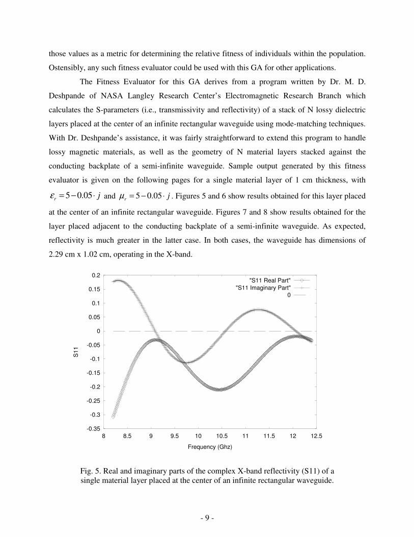
The Fitness Evaluator for this GA derives from a program written by Dr. M. D.

Deshpande of NASA Langley Research Center’ s Electromagnetic Research Branch which

calculates the S-parameters (i.e., transmissivity and reflectivity) of a stack of N lossy dielectric

layers placed at the center of an infinite rectangular waveguide using mode-matching techniques.

With Dr. Deshpande’ s assistance, it was fairly straightforward to extend this program to handle

lossy magnetic materials, as well as the geometry of N material layers stacked against the

conducting backplate of a semi-infinite waveguide. Sample output generated by this fitness

evaluator is given on the following pages for a single material layer of 1 cm thickness, with

5 0.05r jε = − ⋅ and 5 0.05r jµ = − ⋅ . Figures 5 and 6 show results obtained for this layer placed

at the center of an infinite rectangular waveguide. Figures 7 and 8 show results obtained for the

layer placed adjacent to the conducting backplate of a semi-infinite waveguide. As expected,

reflectivity is much greater in the latter case. In both cases, the waveguide has dimensions of

2.29 cm x 1.02 cm, operating in the X-band.

Fig. 5. Real and imaginary parts of the complex X-band reflectivity (S11) of a single material layer placed at the center of an infinite rectangular waveguide.

-0.35

-0.3

-0.25

-0.2

-0.15

-0.1

-0.05

0

0.05

0.1

0.15

0.2

8 8.5 9 9.5 10 10.5 11 11.5 12 12.5

S11

Frequency (Ghz)

"S11 Real Part""S11 Imaginary Part"

0

- 10 -

Fig. 6. Magnitude of the complex X-band reflectivity (in dB) of a single material layer placed at the center of an infinite rectangular waveguide.

Fig. 7. Real and imaginary parts of the complex X-band reflectivity (S11) of a single material layer placed adjacent to the conducting backplate of a semi-infinite, shorted-out waveguide.

-35

-30

-25

-20

-15

-10

-5

8 8.5 9 9.5 10 10.5 11 11.5 12 12.5

S11

(dB

)

Frequency (Ghz)

"S11"

-1

-0.8

-0.6

-0.4

-0.2

0

0.2

0.4

0.6

0.8

1

8 8.5 9 9.5 10 10.5 11 11.5 12 12.5

S11

Frequency (Ghz)

"S11 Real Part""S11 Imaginary Part"

0

- 11 -

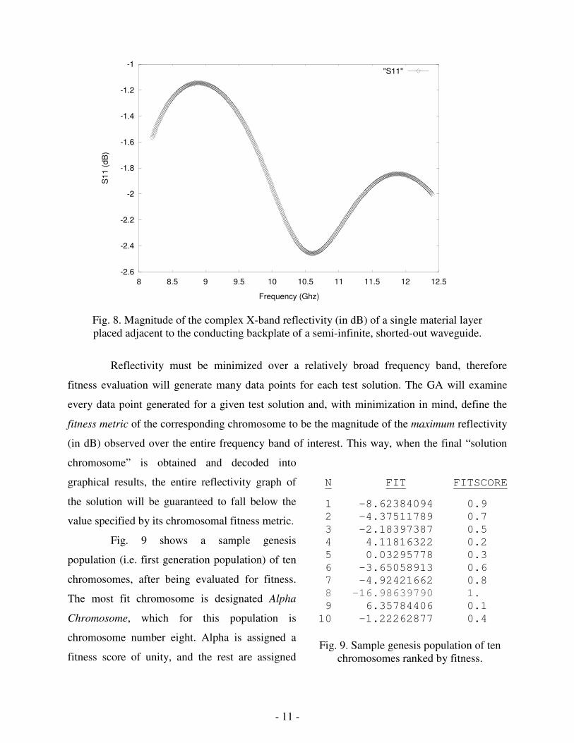
Fig. 8. Magnitude of the complex X-band reflectivity (in dB) of a single material layer placed adjacent to the conducting backplate of a semi-infinite, shorted-out waveguide.

Reflectivity must be minimized over a relatively broad frequency band, therefore

fitness evaluation will generate many data points for each test solution. The GA will examine

every data point generated for a given test solution and, with minimization in mind, define the

fitness metric of the corresponding chromosome to be the magnitude of the maximum reflectivity

(in dB) observed over the entire frequency band of interest. This way, when the final “ solution

chromosome” is obtained and decoded into

graphical results, the entire reflectivity graph of

the solution will be guaranteed to fall below the

value specified by its chromosomal fitness metric.

Fig. 9 shows a sample genesis

population (i.e. first generation population) of ten

chromosomes, after being evaluated for fitness.

The most fit chromosome is designated Alpha

Chromosome, which for this population is

chromosome number eight. Alpha is assigned a

fitness score of unity, and the rest are assigned

-2.6

-2.4

-2.2

-2

-1.8

-1.6

-1.4

-1.2

-1

8 8.5 9 9.5 10 10.5 11 11.5 12 12.5

S11

(dB

)

Frequency (Ghz)

"S11"

N FIT FITSCORE

1 -8.62384094 0.9 2 -4.37511789 0.7 3 -2.18397387 0.5 4 4.11816322 0.2 5 0.03295778 0.3 6 -3.65058913 0.6 7 -4.92421662 0.8 8 -16.98639790 1. 9 6.35784406 0.1 10 -1.22262877 0.4

Fig. 9. Sample genesis population of ten chromosomes ranked by fitness.

- 12 -

fitness scores normalized relative to unity according to their relative fitness rank, as opposed to

their fitness metric. This prevents whatever scale is used for the fitness metric from impacting

the process of natural selection in any way.

It is interesting to note that there is gain associated with some of the chromosomes in

the sample population of Fig. 9. This is a spurious effect arising solely from the fact that the

complex dielectric and magnetic constants of the materials were allowed to take on unphysical

values for the purpose of obtaining the “ fictitious absorber” type ABCs.

VII. Survival of the Most Diverse - Judging quality by fitness alone completely ignores the issue of diversity, which is

defined as the degree to which chromosomes in a population exhibit different genes. Sometimes

in Nature, very unfit-looking individuals and species survive quite well in ecological niches

which lie outside the view of other, more fit-looking individuals and species. The diversity

principle states that it can be just as good to be different as it is to be fit [3]. Equating quality

with fitness alone encourages instances where extremely diverse individuals, which might be

able to contribute greatly to the gene pool, can be completely eliminated just because they have a

fitness metric slightly lower than other individuals who look very much like the rest of the

population. Such termination of unique individuals results in genetic uniformity, thereby

impeding the evolutionary process.

This GA implements a unique method for preserving diversity in populations. Once a

population has been ranked by fitness and the Alpha Chromosome has been identified, the GA

calculates the multidimensional genetic “ distance” between each of the remaining chromosomes

and Alpha. This genetic distance is calculated in exactly the same way as one might calculate the

distance between two points in Euclidean three-space, except there are as many dimensions in

the diversity calculation as there are genes in each chromosome (i.e., 4N for N layers). This

quantity then becomes the diversity metric for each chromosome. Alpha is assigned a diversity

score of unity, since it is the standard against which all others are judged, and the rest of the

chromosomes are assigned diversity scores normalized relative to unity according to their

diversity rank as opposed to their diversity metric, to prevent arbitrary scale issues from

impacting the process of natural selection, as before. Fig. 10 shows the sample population from

Fig. 9 after being evaluated and ranked by fitness and diversity.

- 13 -

VIII. Total Score and Extinction - The initial approach to modeling natural selection was to define each individual’ s total

score, which is the score used for natural selection purposes, as the average of its normalized

fitness and diversity scores, ostensibly incorporating the influence of both criteria when exerting

selection pressure. However, instead of incorporating the influence of the additional selection

criterion (i.e., diversity), empirical investigation demonstrated that the averaging operation

effectively diluted the influence of both selection criteria, slowing down the evolutionary

process, as a whole. Computing total scores as the average of fitness and diversity scores

produced worse convergence than using fitness alone, therefore, another approach was

developed to more robustly incorporate the influence of both.

After much trial-and-error, the best convergence was obtained when each generation was

randomly evaluated for extinction using either fitness or diversity as a selection criterion, but not

both. A “ digital coin toss” for each generation uniquely determines with equal probability

whether fitness or diversity will be used as the selection criterion for that generation’ s

population. Once the determination is made, each individual’ s total score is set equal to either its

fitness score or its diversity score. Then, all individuals having total scores which do not meet or

exceed the extinction criterion, which is the minimum total score necessary for survival, are

extinguished. The effects of both selection criteria are preserved, and much swifter convergence

is obtained compared to that obtained by repetitively using either criterion alone or both criteria

simultaneously, generation after generation.

N FIT FITSCORE DIV DIVSCORE

1 -8.62384094 0.9 21.8770694 0.5 2 -4.37511789 0.7 21.4814842 0.4 3 -2.18397387 0.5 19.539844 0.2 4 4.11816322 0.2 25.7370131 0.8 5 0.03295778 0.3 22.2742858 0.7 6 -3.65058913 0.6 25.7379826 0.9 7 -4.92421662 0.8 19.4708345 0.1 8 -16.98639790 1. 1.e+100 1. 9 6.35784406 0.1 19.6973937 0.3 10 -1.22262877 0.4 22.2196678 0.6

Fig. 10. Sample population of ten chromosomes ranked by fitness and diversity.

- 14 -

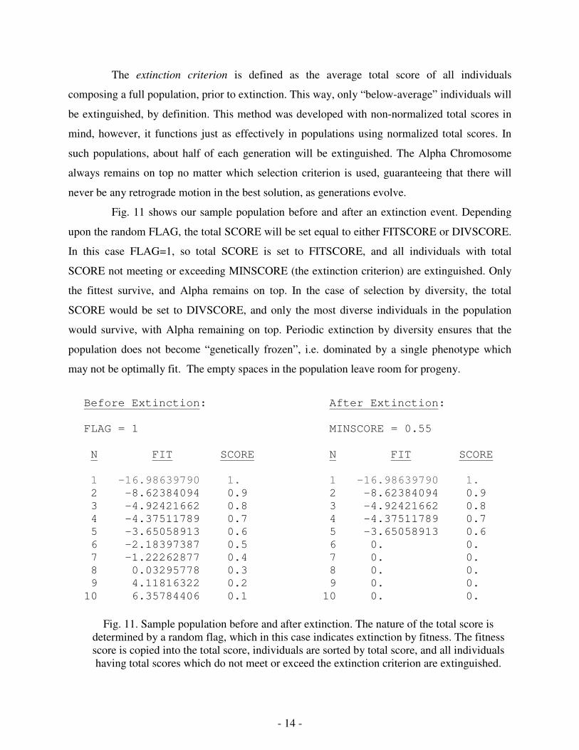
The extinction criterion is defined as the average total score of all individuals

composing a full population, prior to extinction. This way, only “ below-average” individuals will

be extinguished, by definition. This method was developed with non-normalized total scores in

mind, however, it functions just as effectively in populations using normalized total scores. In

such populations, about half of each generation will be extinguished. The Alpha Chromosome

always remains on top no matter which selection criterion is used, guaranteeing that there will

never be any retrograde motion in the best solution, as generations evolve.

Fig. 11 shows our sample population before and after an extinction event. Depending

upon the random FLAG, the total SCORE will be set equal to either FITSCORE or DIVSCORE.

In this case FLAG=1, so total SCORE is set to FITSCORE, and all individuals with total

SCORE not meeting or exceeding MINSCORE (the extinction criterion) are extinguished. Only

the fittest survive, and Alpha remains on top. In the case of selection by diversity, the total

SCORE would be set to DIVSCORE, and only the most diverse individuals in the population

would survive, with Alpha remaining on top. Periodic extinction by diversity ensures that the

population does not become “ genetically frozen” , i.e. dominated by a single phenotype which

may not be optimally fit. The empty spaces in the population leave room for progeny.

Before Extinction: After Extinction: FLAG = 1 MINSCORE = 0.55 N FIT SCORE N FIT SCORE 1 -16.98639790 1. 1 -16.98639790 1. 2 -8.62384094 0.9 2 -8.62384094 0.9 3 -4.92421662 0.8 3 -4.92421662 0.8 4 -4.37511789 0.7 4 -4.37511789 0.7 5 -3.65058913 0.6 5 -3.65058913 0.6 6 -2.18397387 0.5 6 0. 0. 7 -1.22262877 0.4 7 0. 0. 8 0.03295778 0.3 8 0. 0. 9 4.11816322 0.2 9 0. 0. 10 6.35784406 0.1 10 0. 0.

Fig. 11. Sample population before and after extinction. The nature of the total score is determined by a random flag, which in this case indicates extinction by fitness. The fitness score is copied into the total score, individuals are sorted by total score, and all individuals having total scores which do not meet or exceed the extinction criterion are extinguished.

- 15 -

A A

B B

C E

D D

E C

F F

Fig. 13. Mitosis with chain reversal.

IX. Propagation of the Species - The process of extinction leaves vacancies in the population which must be filled.

These vacancies are filled using numerical analogues of reproduction, providing mechanisms for

genetic recombination whereby new individuals (i.e. “ children” ) are created that have a chance

to be more fit than their parents. Since total scores are normalized, half of the population will be

killed off during each extinction, requiring creation of exactly as many replacements as there are

individuals left in the population after each extinction. This uniquely symmetric result

guarantees every survivor a chance to produce a child for the next generation, therefore every

survivor reproduces at least once, in this GA. Reproduction may be asexual or sexual, and if

reproduction is sexual, then the survivor’ s mate is chosen randomly from the other survivors,

with probability of selection weighted by total score. Reproduction can occur in any of four

possible ways, with equal probability:

¾�Mitosis -

Mitosis is an asexual cell division process in

which the nucleus divides, normally resulting in two

new cells, each of which contains a complete copy

of the parental chromosomes. Essentially, the

individual selected for mitosis creates a clone of

itself in the population. The clone will be subject to

the possibility of mutation during the next phase of

the evolutionary process, but the parent will not.

¾�Mitosis with Chain Reversal -

An asexual cell division process similar to

mitosis, with one major difference. Chain reversal

is a chromosomal aberration which occurs during

replication when a subdomain of the original

chromosome detaches, reverses polarity, and

reattaches at opposite ends, forming a new

chromosome.

A A

B B

C C

D D

E E

F F

Fig. 12. Mitosis.

- 16 -

Chain reversal can occur on a chromosomal subdomain as small as a single pair of

genes or as large as the entire chromosome, and it always produces a child which is

uniquely different from the parent. Like the mitotic clone before, this child will also be

subject to the possibility of mutation during the next phase of the evolutionary process,

but its parent will not.

¾�N-Point Crossing Over -

Crossing over is genetic recombination arising from the sexual reproduction of two

parents. When parent chromosomes come together during the process of reproduction,

genetic material is exchanged between them in the vicinity of one or more points of

contact. One such point, known as the centromere, is that place where the midpoints of

two parent haploid chromosomes join so that the pair looks like the letter “ X” . There

may also be other points of contact along the chromosomal chain known as chiasma. In

this GA, the minimum number of crossover points is one (always at the centromere), and

the maximum number of crossover points cannot exceed one-half the total number of

genes in each chromosome. Chiasma may be located anywhere along the chromosomal

chain, and the locations of these points in conjunction with the centromere are used to

define distinct chromosomal subdomains, on which genetic information is exchanged

between parents to form the blueprint of a new individual.

A 1 A 1 A 1

B 2 B 2 B 2

C 3 C 3 3 C

D 4 D 4 4 D

E 5 E 5 E 5

F 6 F 6 F 6

G 7 G 7 G 7

H 8 H 8 H 8

Fig. 14. 2-Point crossing over involving the centromere and one chiasm. Genes within one subdomain are exchanged between parents.

- 17 -

The source of genetic material alternates on each subdomain, with Parent 1 contributing

to all odd subdomains and Parent 2 contributing to all even subdomains. Although two

children could be created using this method, in this GA only one child is created and

propagated to the next generation. The question of which child to propagate is arbitrary,

depending solely upon which chromosomes are defined as Parent 1 and Parent 2.

¾�“ Channeled” Crossing Over -

Channeled crossover is also the result of sexual reproduction between two parents. This

recombination strategy exploits the specific chromosomal encoding pattern unique to this

application. Examination of section III. above shows that the primed and double-primed

values of all variables encoded within each chromosome alternate regularly along the

chromosomal chain. The process of “ channeled” crossover randomly selects two

breakpoints on the chromosomal chain and exchanges every other gene along this

subdomain between parents, to beget progeny. It is reasonable to assume that real

problems may impose very different constraints upon primed and unprimed quantities.

This type of crossover offers a unique opportunity for individuals doing well in the

primed dimensions to unite with individuals doing well in the unprimed dimensions. As

before, only one child is created and propagated to the next generation. The question of

which child to propagate is completely arbitrary, depending on the definition of parents.

A 1 A 1 A 1

B 2 B 2 B 2

C 3 C 3 C 3

D 4 D 4 4 D

E 5 E 5 E 5

F 6 F 6 6 F

G 7 G 7 G 7

H 8 H 8 H 8

Fig. 15. Channeled crossover between two parents on a chromosomal subdomain of length four.

- 18 -

X. Hybridization - Once the population has been replenished through reproduction, there exists the

possibility that one or more offspring may contain gene values lying outside constraints specified

by the input file. One particular reproduction operation that could produce this effect is mitosis

with chain-reversal. Such genetic defects are relatively infrequent in this GA, occurring in only

eight percent of genes expressed in offspring, on average. Nevertheless, that is frequent enough

to necessitate that some method be implemented to correct these defects within progeny after

reproduction, once they have already been written into the population.

After all children are born, this GA examines each child for genetic defects (i.e. gene

values which lie outside specified constraints). If one is found, the GA will excise that gene from

the chromosome in question and artificially replace it with the corresponding gene from the

current Alpha Chromosome, creating a transgenic hybrid. This process, which is analogous to

recombinant genetic engineering (as might be implemented within a biological laboratory),

ensures that all genes in the new population fall within constraints specified by the input file

before being propagated to the next generation for fitness evaluation. The rationale underlying

this operation is that Alpha should always donate the very best gene available, because it is the

fittest individual in the population. Although it would seem reasonable that this practice might

promote crippling uniformity in the population, the consistent inclusion of diversity as a

selection criterion, as well as the infrequent necessity of such artificial recombinations seems to

successfully offset any tendency toward uniformity.

It should be noted that other potential strategies for handling this situation include

random generation of a new gene whenever an outlier is found, or simply omitting reproductive

processes which give rise to such defects in the first place. However, correction by hybridization

using genetic material donated by Alpha consistently produced significantly faster convergence.

XI. Mutation -

Mutation is the random environmental perturbation of one or more genes within the

chromosomal chain of an individual which may alter its phenotype, thereby giving it a greater or

lesser advantage in the process of natural selection. The vast majority of mutations are

unfavorable, however, the occasional mutant may actually be more fit than the species from

whence it arose, enabling its propagation and subsequent introduction of new genetic material

- 19 -

into the population. This process drives variation of the species in nature. In an evolutionary

simulation, mutation operators provide analogous numerical mechanisms for introducing new

“ genetic material” into the population, thereby enabling full exploration of the search space.

Naturally, it is a good idea to protect the fittest individuals (i.e. solutions) in the

population from the damaging effects of mutation, therefore mutation isn’ t allowed to affect the

parents of a given generation; it can only affect their children. Once children are checked for

mutations, the newly-created population becomes a new generation of its own, starting another

iteration of the evolutionary process beginning with fitness evaluation.

The mutation probability determines the frequency with which gene values will be

changed. If the mutation rate is too low, then new traits will appear too slowly in the population

to obtain convergence in any reasonable number of generations. Conversely, if the mutation rate

is too high, then each generation of children will bear little or no resemblance to their parents,

and the entire algorithm will degenerate into a crude random search. In this GA, the mutation

probability is calculated as unity minus the average total score of all individuals surviving

extinction (i.e., the parents only). This way, if the average fitness of survivors is high, then

mutation rate will be low, and if the average fitness of survivors is low, then the mutation rate

will be high. This tends to stimulate variation in the species when necessary, and tends to

suppress the potentially damaging effects of mutation on the children of a very fit group of

survivors. Although this formula for the mutation probability was originally developed with non-

normalized total scores in mind, it functions properly when total scores are normalized, as well.

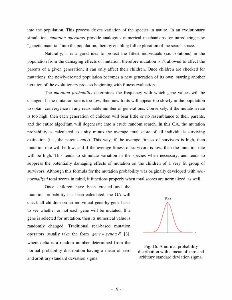
Once children have been created and the

mutation probability has been calculated, the GA will

check all children on an individual gene-by-gene basis

to see whether or not each gene will be mutated. If a

gene is selected for mutation, then its numerical value is

randomly changed. Traditional real-based mutation

operators usually take the form gene gene δ= ± [3],

where delta is a random number determined from the

normal probability distribution having a mean of zero

and arbitrary standard deviation sigma.

Fig. 16. A normal probability

distribution with a mean of zero and arbitrary standard deviation sigma.

- 20 -

This particular algorithm foregoes the additive mutation operator in favor of two other

mutation operators, each having a unique mathematical form and method of determining sigma.

A proper choice of sigma, the standard deviation of the normal distribution, is critical for

successful mutation. Sigma determines the width of the normal distribution, thereby constraining

the most likely order of magnitude of the random numbers generated. In theory, sigma should be

large at the start of the algorithm and then decrease as the algorithm converges, so variability

will be favored during the early stages of evolution but the damaging effects of mutation on

nearly optimal solutions will be mitigated. Certainly, different choices of sigma produce

radically different evolutionary behaviors, and fine-tuning sigma to adapt properly to the

progress of the evolutionary simulation can be extremely difficult. When this GA determines that

a gene must be mutated, it will randomly select one of the following operators, with equal

probability of each. If a mutation would carry a gene outside specified constraints, the mutation

is ignored as if it never happened:

¾�Mutiplicative Operator -

This mutation operator has the form gene gene δ= ∗ where delta is a random multiplier

determined from the normal probability distribution having a mean of 1.0, and sigma

GHWHUPLQHG� DV�� � � ��� – (Current Best Fitness) / (Target Fitness). This way, delta will

randomly fluctuate around unity, presenting mutated genes with an equal probability of

increasing or decreasing, on average. The magnitude of that increase or decrease will be

determined by a value of sigma which adapts to the progress of the algorithm. Sigma begins

as unity at the first generation and then decreases linearly, approaching zero as the “ current

best fitness” (i.e., the fitness metric of the current Alpha Chromosome) approaches the

desired target fitness. Since the target fitness is specified by keyboard input, it is easy to

change the slope of linear decrease in sigma by simply specifying a different target fitness.

¾�Perturbative Operator -

This operator perturbs genetic values by replacing the original gene with a slightly

different value, determined from the normal probability distribution having a mean equal to

the original gene value, and an adaptive value of sigma. The distribution now randomly

fluctuates around the original gene value relatively tightly, and the influence of sigma is

more absolute. The adaptive value of sigma is determined as follows:

- 21 -

Whenever a newer, fitter Alpha Chromosome replaces an older, less fit one, an integer

FRXQWHU� �FDOO� LW� «�� LV� VHW� HTXDO� WKH� FXUUHQW� JHQHUDWLRQ�QXPEHU��$V� WKH� JHQHUDWLRQ�QXPEHU�increases, the value of each generation is successively adGHG�WR� ��DQG�VLJPD�LV�FDOFXODWHG�DV�WKH�FXUUHQW�JHQHUDWLRQ�QXPEHU�GLYLGHG�E\� �� To see how this works, consider two generations with no improvement in the solution.

2Q�JHQHUDWLRQ���� � ����DQG�WKHUHIRUH� � ����2Q�JHQHUDWLRQ���� � ��������DQG� � ��������, or

�������1RZ��RQ�JHQHUDWLRQ����OHW�D�QHZ�$OSKD�&KURPRVRPH�EH�IRXQG��$V�D�FRQVHTXHQFH�� �LV�VHW�HTXDO�WR�WKUHH��DQG� � ������RU����2Q�JHQHUDWLRQ����WKHUH�LV�QR�FKDQJH��WKHUHIRUH� � ��������DQG� � ����������RU�������7KLV�PHWKRG�RI�FDOFXODWLQJ�VLJPD�LQVXUHs that it always begins as

unity whenever a new Alpha Chromosome is found, and asymptotically decreases to zero

more and more quickly after each replacement of the Alpha Chromosome.

Essentially, the algorithm attempts progressively smaller perturbations of the genetic

values selected for mutation as generations progress, until one is found (almost by “ brute

force” ) which yields a better solution. As generations increase, the asymptotic dropoff

becomes steeper and steeper, so that less effort is expended using larger values of sigma in

the late stages of evolution without having to abandon the use of large values entirely. Sigma

now determines an absolute magnitude of perturbation, and it may be scaled to a range

appropriate for each specific application by using a multiplier, if desired. Fig. 17 shows the

progression of sigma over 20 generations using this method (without scaling), assuming that

a new Alpha Chromosome is discovered at the tenth generation.

Fig. 17. Standard Deviation of the Perturbative Mutator.

0

0.2

0.4

0.6

0.8

1

2 4 6 8 10 12 14 16 18 20

Sig

ma

Generation

"SigData"0.1820.129

- 22 -

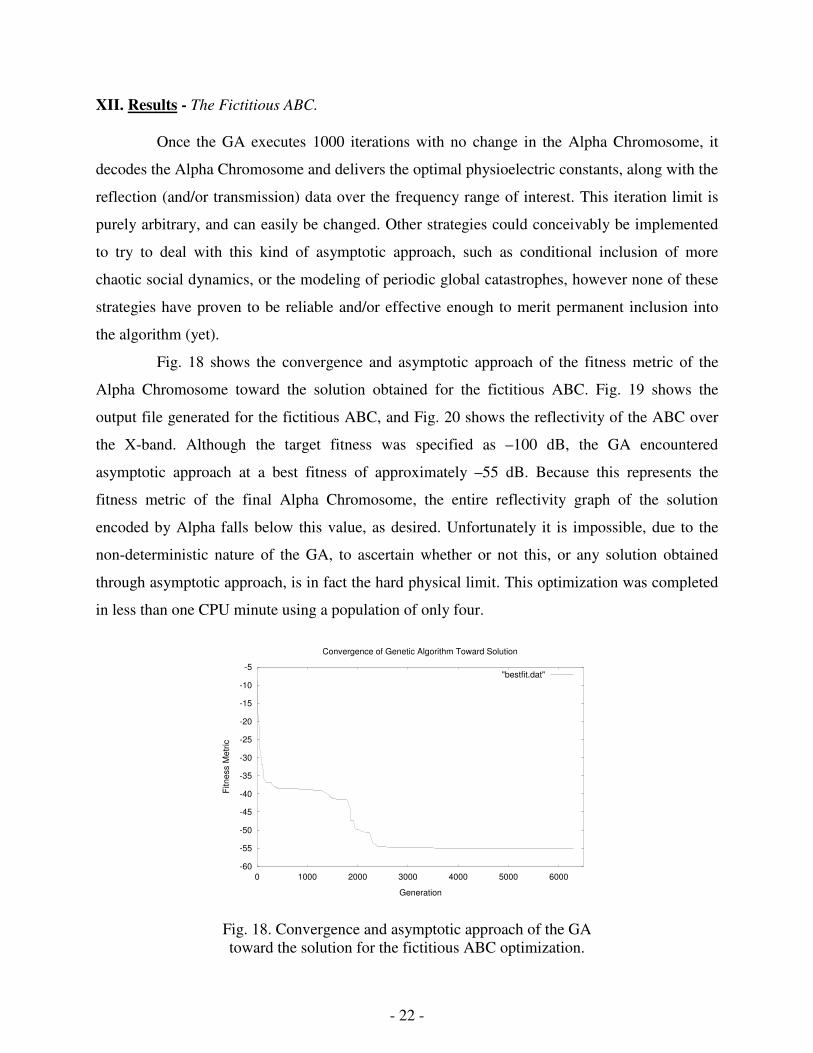
XII. Results - The Fictitious ABC. Once the GA executes 1000 iterations with no change in the Alpha Chromosome, it

decodes the Alpha Chromosome and delivers the optimal physioelectric constants, along with the

reflection (and/or transmission) data over the frequency range of interest. This iteration limit is

purely arbitrary, and can easily be changed. Other strategies could conceivably be implemented

to try to deal with this kind of asymptotic approach, such as conditional inclusion of more

chaotic social dynamics, or the modeling of periodic global catastrophes, however none of these

strategies have proven to be reliable and/or effective enough to merit permanent inclusion into

the algorithm (yet).

Fig. 18 shows the convergence and asymptotic approach of the fitness metric of the

Alpha Chromosome toward the solution obtained for the fictitious ABC. Fig. 19 shows the

output file generated for the fictitious ABC, and Fig. 20 shows the reflectivity of the ABC over

the X-band. Although the target fitness was specified as –100 dB, the GA encountered

asymptotic approach at a best fitness of approximately –55 dB. Because this represents the

fitness metric of the final Alpha Chromosome, the entire reflectivity graph of the solution

encoded by Alpha falls below this value, as desired. Unfortunately it is impossible, due to the

non-deterministic nature of the GA, to ascertain whether or not this, or any solution obtained

through asymptotic approach, is in fact the hard physical limit. This optimization was completed

in less than one CPU minute using a population of only four.

Fig. 18. Convergence and asymptotic approach of the GA toward the solution for the fictitious ABC optimization.

-60

-55

-50

-45

-40

-35

-30

-25

-20

-15

-10

-5

0 1000 2000 3000 4000 5000 6000

Fitn

ess

Met

ric

Generation

Convergence of Genetic Algorithm Toward Solution

"bestfit.dat"

- 23 -

******** PARAMETERS ********** ***************************** A = 2.29 B = 1.02 Population = 4 NLAYERS = 3 Generations = 7284 FSTART = 8.2 Bestfit = -55.1051287 FEND = 12.4 CPU Time = 0.891666667 minutes. FSTEP = 0.1 ********* LAYER 1 ************ ********* LAYER 3************ Z = 0. Z = 0.2 E’ = -5.81435204 E’ = 1.24189401 E’’ = 7.9716177 E’’ = 1.19435549 M’ = -8.3258419 M’ = 8.84083939 M’’ = 9.08495998 M’’ = 2.78866553 ********* LAYER 2************ ********* LAYER 4************ Z = 0.1 Z = 0.3 E’ = 7.82274437 E’ = 0. E’’ = -8.25729847 E’’ = 0. M’ = 3.17915225 M’ = 0. M’’ = -3.83381701 M’’ = 0. ***************************** *****************************

Fig. 19. Output file for the fictitious 3-layer ABC. Physioelectric constants take the form of (primed value) – j * (double primed value). For example, epsilon for layer 2 is (7.82 + j * 8.26). It is interesting to note that the first layer is composed of a double-negative, or meta-material.

Fig. 20. Magnitude of the X-band reflectivity (in dB) of the fictitious 3-layer ABC.

-80

-75

-70

-65

-60

-55

-50

8 8.5 9 9.5 10 10.5 11 11.5 12 12.5

S11

(dB

)

Frequency (Ghz)

X-Band Reflectivity of Fictitious 3-Layer Absorbing Boundary Conditions

-55.1051287"s11db.out"

- 24 -

The fictitious 3-layer ABC was validated using multiple test cases. As an example, Fig.

21 shows the performance of the fictitious ABC used in conjunction with the single magneto-

dielectric slab of 1 cm thickness having 5 0.05r jε = − ⋅ and 5 0.05r jµ = − ⋅ , which was

analyzed in section VI. The performance of the fictitious ABC used in conjunction with this

dielectric slab is compared to the reflectivity of the slab backed by free space. The “ Slab Open”

case, indicated by the solid black line, shows the reflectivity of the dielectric slab placed at the

center of an infinitely long waveguide, as shown in Fig. 6. The “ Slab Shorted” case, indicated by

the dashed line, shows the reflectivity of the same slab placed against the perfectly conducting

backplate of a semi-infinite, shorted-out waveguide, as shown in Fig. 8. As expected, reflectivity

is much higher in this case. The “ Slab Shorted With ABC” case, indicated by large diamonds,

shows the reflectivity of the slab backed by the fictitious 3-layer absorber, clearly demonstrating

that backing the slab with the 3-layer ABC is numerically equivalent to backing it with free

space, even though the ABC includes a PEC enclosure. The average error produced by backing

the test case with the ABC relative to backing the test case with free space was 0.23%.

Fig. 21. Efficacy of fictitious ABCs obtained using the GA.

-35

-30

-25

-20

-15

-10

-5

0

5

8 8.5 9 9.5 10 10.5 11 11.5 12 12.5

S11

(dB

)

Frequency (Ghz)

Efficacy of Fictitious Absorbing Boundary Conditions

"Slab Open""Slab Shorted"

"Slab Shorted With ABC"

- 25 -

Fig. 22. Using fictitious ABCs within a complete PEC enclosure could be useful for terminating open-region FEM meshes. This conjecture has not yet been tested using FEM.

XIII. Results - Real Absorbers. Satisfactory performance of Radar Absorbing Materials (RAM) requires getting the

maximum amount of radiofrequency energy into the RAM as possible, and then providing a

sufficient amount of loss to absorb that energy within the allowed thickness. Unfortunately, very

lossy materials usually have impedances that are very different than free space, producing high

reflection at the free space boundary. This issue complicates deterministic RAM design.

Although intended for development of fictitious absorbers, this GA can also be used to

design real Radar Absorbing Materials by specifying realistic constraints corresponding to

whatever materials will be used to fabricate the multilayered structure. The problem then reduces

to minimization of the reflectivity of an arbitrary number of homogeneous, lossy dielectric or

magnetic layers of arbitrary thickness positioned adjacent to the perfectly conducting backplate

of a semi-infinite, shorted-out rectangular waveguide.

The performance of this GA was analyzed over a broad range of realistic absorber

design problems. The initial study attempted to minimize reflection using up to ten layers of

1mm-thick non-magnetic dielectric material, with each layer subject to the following constraints: ’1 10rε≤ ≤ and ’’0 10rε≤ ≤ . Fig. 23 shows the maximum X-band reflectivity as a function of the

number of layers used. The X-band reflectivity curve for a given stack will fall entirely below the

value indicated in Fig. 23. Asymptotic behavior is clearly observed. Fig. 24 extends this analysis

to permit the dielectric materials to become magnetic as well, subject to the same dielectric

constraints as above, plus: ’1 10rµ≤ ≤ , and ’’0 10rµ≤ ≤ . A quasi-odd-even effect is observed.

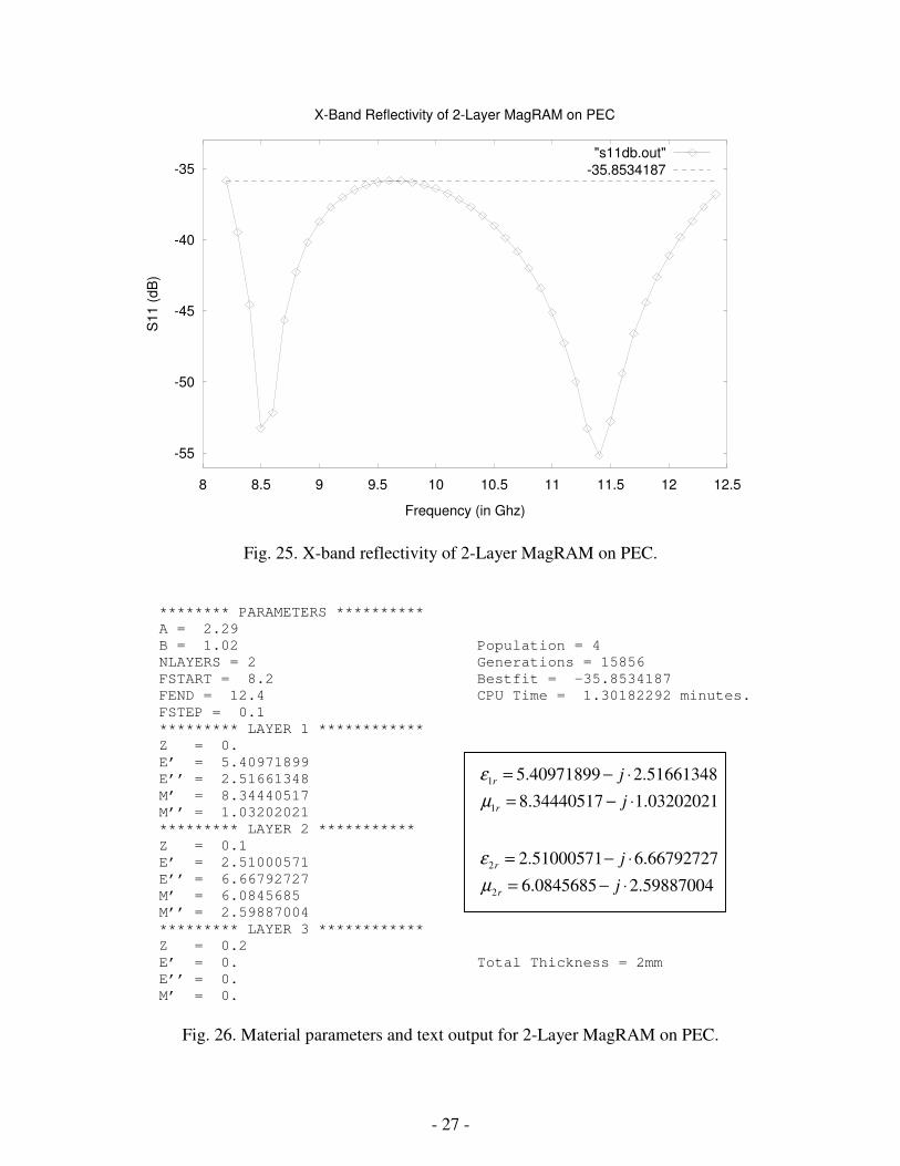
Figures 25 and 26 show results obtained for 2-layer MagRAM on PEC consisting of

two layers of custom material bonded to metal, having a total thickness of two millimeters and

providing a minimum X-band RCSR of approximately 36 “ dB down” within the waveguide.

Free Free Space Space

Test Case

∞ ∞

Test Case

- 26 -

Fig. 23. Maximum X-band reflectivities of realistic multilayer dielectric absorbers.

Fig. 24. Maximum X-band reflectivities of realistic multilayer magneto-dielectric absorbers.

-30

-25

-20

-15

-10

-5

0

5

0 2 4 6 8 10

S11

Max

(dB

)

Number of Layers

Maximum X-Band Reflectivities of Realistic Multilayer Lossy Dielectric Absorbing Material

"Fitness Metric"

-44

-42

-40

-38

-36

-34

-32

-30

-28

-26

-24

0 2 4 6 8 10

S11

Max

(dB

)

Number of Layers

Maximum X-Band Reflectivities of Realistic Multilayer Lossy Magneto-Dielectric Absorber

"Fitness Metric"

This looks promising.

- 27 -

Fig. 25. X-band reflectivity of 2-Layer MagRAM on PEC.

******** PARAMETERS ********** A = 2.29 B = 1.02 Population = 4 NLAYERS = 2 Generations = 15856 FSTART = 8.2 Bestfit = -35.8534187 FEND = 12.4 CPU Time = 1.30182292 minutes. FSTEP = 0.1 ********* LAYER 1 ************ Z = 0. E’ = 5.40971899 E’’ = 2.51661348 M’ = 8.34440517 M’’ = 1.03202021 ********* LAYER 2 *********** Z = 0.1 E’ = 2.51000571 E’’ = 6.66792727 M’ = 6.0845685 M’’ = 2.59887004 ********* LAYER 3 ************ Z = 0.2 E’ = 0. Total Thickness = 2mm E’’ = 0. M’ = 0.

Fig. 26. Material parameters and text output for 2-Layer MagRAM on PEC.

-55

-50

-45

-40

-35

8 8.5 9 9.5 10 10.5 11 11.5 12 12.5

S11

(dB

)

Frequency (in Ghz)

X-Band Reflectivity of 2-Layer MagRAM on PEC

"s11db.out"-35.8534187

1

1

5.40971899 2.51661348

8.34440517 1.03202021r

r

j

j

εµ

= − ⋅= − ⋅

2

2

2.51000571 6.66792727

6.0845685 2.59887004r

r

j

j

εµ

= − ⋅= − ⋅

- 28 -

XIV. Conclusion - Traditionally, successful RAM design requires familiarity with the types of materials

available, good engineering judgment, and thorough knowledge of RAM performance. In this

work, elements of Darwin’ s Theory of Evolution were modeled algorithmically to implement a

novel, real-based Genetic Algorithm for the non-deterministic optimization and design of Radar

Absorbing Materials. Although typical Genetic Algorithms require populations of many

thousands in order to function properly and obtain correct results, verified correct results were

obtained within a reasonable time interval using this GA with a population of only four.

Although the algorithm described herein was designed optimize, it is by no means

optimal. Obtaining the most favorable combination of operators and their associated probabilities

requires extensive trial-and-error, which is an extremely time-consuming process. This work

merely represents the current best draft obtainable within the time allocated for its development

and is still a work in progress, not unlike any given generation of the organisms it models. This

GA could probably be vastly improved and even better results obtained if the work were

extended. In conclusion, it is, perhaps, most important to point out that although this report

describes one particular application of the GA, any fitness evaluator could be used with this GA

for different applications.

XV. Acknowledgements – The author would like to gratefully acknowledge Dr. Patrick Henry Winston, whose

instructive text “ Artificial Intelligence” [3] served as the foundation of the AI work reported

herein. There is no adequate way to reference how much this text contributed to the completion

of this work. The author would also like to gratefully acknowledge Dr. M. D. Deshpande of the

NASA Langley Research Center for providing his mode-matching code, and Dr. Gregory

Wilkins of Morgan State University for his illuminating discourse on the electromagnetic theory

of waveguides.

- 29 -

XVI. References -

1. Darwin, Charles Robert. The Origin of Species. Vol. XI. The Harvard Classics. New

York: P.F. Collier & Son, 2001.

2. Holland, John H. Adaptation in Natural and Artificial Systems. Ann Arbor, MI.: The

University of Michigan Press, 1975.

3. Winston, Patrick H. Artificial Intelligence. 3rd ed. Addison Wesley, 1993.

4. Antonisse, J. A new interpretation of schema notation that overturns the binary encoding

constraint. In Proceedings of the Third International Conference on Genetic Algorithms,

1989.

5. Chandler, R. and Northrop, P. http://www.ucl.ac.uk/~ucakarc/work/randgen.html.

6. Marsaglia, G. & Zaman, A. A new class of random number generators. Annals of

Applied Probability, vol. 1, pp.462-480, 1991.

- 30 -

XVII. Appendix – Genetic Algorithm Flowchart.

Create “ Genesis” Population

Determine the Normalized Fitness Score of Each Individual

Determine the Normalized Diversity Score of Each Individual

With P = 0.5 for each:

Sort by Fitness OR Sort by Diversity

Extinguish Below-Average Individuals

Force Each Parent to Produce a Child

With P = 0.25 for each: Mitosis without OR Mitosis with OR N-Point OR Channeled Chain-Reversal Chain-Reversal Crossover Crossover

Hybridize to Correct Genetic Defects in Children

Check Each Child for Mutation

Has the Target Fitness Been Reached?

No Yes

Terminate

REPORT DOCUMENTATION PAGE Form ApprovedOMB No. 0704-0188

2. REPORT TYPE

Contractor Report 4. TITLE AND SUBTITLE

A Novel, Real-Valued Genetic Algorithm for Optimizing Radar Absorbing Materials

5a. CONTRACT NUMBER

NAS1-00135

6. AUTHOR(S)

Hall, John Michael

7. PERFORMING ORGANIZATION NAME(S) AND ADDRESS(ES)

NASA Langley Research Center Lockheed Martin Space OperationsHampton, VA 23681-2199 Hampton, VA 23681-2199

9. SPONSORING/MONITORING AGENCY NAME(S) AND ADDRESS(ES)

National Aeronautics and Space AdministrationWashington, DC 20546-0001

8. PERFORMING ORGANIZATION REPORT NUMBER

10. SPONSOR/MONITOR'S ACRONYM(S)

NASA

13. SUPPLEMENTARY NOTESLangley Technical Monitor: M. D. DeshpandeAn electronic version can be found at http://techreports.larc.nasa.gov/ltrs/ or http://ntrs.nasa.gov

12. DISTRIBUTION/AVAILABILITY STATEMENTUnclassified - Un�imitedSubject Cate�ory 33Availability� NASA CASI (301) 6�1-0390 Dist�ibution: Standard

19a. NAME OF RESPONSIBLE PERSON

STI Help Desk (email: help@sti.nasa.gov)

14. ABSTRACT

A novel, real�-valued Genetic Algorithm (GA) was designed and implemented to minimize the reflectivity and/or transmissivity of an arbitrary number of homogeneous, lossy dielectric or magnetic layers of arbitrary thickness positioned at either the center of an infinitely long rectangular waveguide, or adjacent to the perfectly conducting backplate of a semi-infinite, shorted-out rectangular waveguide. Evolutionary processes extract the optimal physioelectric constants falling within specified constraints which minimize reflection and/or transmission over the frequency band of interest. This GA extracted the unphysical dielectric and magnetic constants of three layers of fictitious material placed adjacent to the conducting backplate of a shorted-out waveguide such that the reflectivity of the configuration was –55 dB or less over the entire X-band. Examples of the optimization of realistic multi-layer absorbers are also presented. Although typical Genetic Algorithms require populations of many thousands in order to function properly and obtain correct results, verified correct results were obtained for all test cases using this GA with a population of only four.

15. SUBJECT TERMS

Artificial Intelligence, Genetic Algorithms, Radar Abosrbing Materials

18. NUMBER OF PAGES

35

19b. TELEPHONE NUMBER (Include area code)

(301) 621-0390

a. REPORT

U

c. THIS PAGE

U

b. ABSTRACT

U

17. LIMITATION OF ABSTRACT

UU

Prescribed by ANSI Std. Z39.18Standard Form 298 (Rev. 8-98)

3. DATES COVERED (From - To)

5b. GRANT NUMBER

5c. PROGRAM ELEMENT NUMBER

5d. PROJECT NUMBER

5e. TASK NUMBER

5f. WORK UNIT NUMBER

706-31-41-01

11. SPONSOR/MONITOR'S REPORT NUMBER(S)

NASA/CR-2004-212669

16. SECURITY CLASSIFICATION OF:

The public reporting burden for this collection of information is estimated to average 1 hour per response, including the time for reviewing instructions, searching existing data sources, gathering and maintaining the data needed, and completing and reviewing the collection of information. Send comments regarding this burden estimate or any other aspect of this collection of information, including suggestions for reducing this burden, to Department of Defense, Washington Headquarters Services, Directorate for Information Operations and Reports (0704-0188), 1215 Jefferson Davis Highway, Suite 1204, Arlington, VA 22202-4302. Respondents should be aware that notwithstanding any other provision of law, no person shall be subject to any penalty for failing to comply with a collection of information if it does not display a currently valid OMB control number.PLEASE DO NOT RETURN YOUR FORM TO THE ABOVE ADDRESS.

1. REPORT DATE (DD-MM-YYYY)

03 - 200401-