JOURNAL OF CCXAPUlAlIONAl. AND APPLIED MATHEMATICS

Journal of Computational and Applied Mathematics 94 (1998) 55-67

A numerical algorithm for the solution of Signorini problems

J.M. Aitchison*, M.W. Poole Applied Mathematics and Operational Research Group, Cranjeld University, RMCS Shrivenham, Swindon,

SN6 8LA, UK

Received 2 October 1996; received in revised form 3 December 1997

Abstract

In this paper we propose a new iterative algorithm for the solution of a certain class of Signorini problems. Such problems arise in the modelling of a variety of physical phenomena and usually involve the determination of an unknown free boundary. Here we describe a way of locating the free boundary directly and provide a proof that the algorithm converges when used with analytic methods. The advantage of this algorithm is that it can be used in conjunction with any numerical method with minimal development of extra code. We demonstrate its application with the boundary element method to some physical problems in both two and three dimensions. @ 1998 Elsevier Science B.V. All rights reserved.

AMS classification: 65N38, 35R35

Keywords: Signorini; Free boundary problems; Boundary element methods; Complementarity relations

1. Introduction

A Signorini-type problem is one in which the boundary conditions for a governing partial dif- ferential equation are in the form of inequalities involving the unknown function and its derivative together with a complementarity relation. Such boundary conditions are often referred to as being unilateral. In 1933, Signorini [ 151 studied a contact problem in elasticity with unilateral boundary conditions from which the term Signorini problem was coined. (For a more recent reference consult Glowinski [6]. )

Not surprisingly, most Signorini problems occur in contact problems where we have two or more objects colliding. Typically, boundary conditions are of the form

24” - s < 0, r, < 0, Z,(U, - s) = 0

* Corresponding author.

0377~0427/98/$19.00 @ 1998 Elsevier Science B.V. All rights reserved Z’ZZ SO377-0427(98)00030-2

56 J.M. Aitchison, M. W. Poole1 Journal of Computational and Applied Mathematics 94 (1998) 5567

applying on the contact part of the boundary. Here u, is the displacement in the direction of the outward normal to the contact surface and r, is the component of the Cauchy stress tensor in the normal direction. The distance between the contact surface and the obstacle (possibly another moving body) is given by s, which may be a given positive function. The case

u,=s and r,<O

represents the two objects being in the contact whilst the case

u,<s and r,=O

occurs when the two objects are not in contact. Such boundary conditions problems are often referred to as nonpenetration conditions. Examples of found in [9, 10, 121.

in the context of contact contact problems can be

More general Signorini problems are sometimes referred to as thin-obstacle problems [4], where the conditions on the boundary are, for example,

where 4 is the unknown function to be determined and where f and g may be given functions of position and are known as thin obstacles. Problems of this type studied in the literature include the electropaint problem ([2], the shallow dam problem [ 11) and some optimal shape design problems considered by Neittaanmaki [ 111 and Haslinger [7].

It is known (for example, see [6]) that Signorini problems such as these can be recast as variational inequalities and hence can be solved directly by the finite element method (FEM). Its ease in dealing with the problems posed by the inequality boundary conditions has made the FEM the most popular numerical method for solving Signorini problems and is the basis of the numerical methods used by all of the authors mentioned above. However, in these problems the primary interest is in some or all of the boundary making them ideal candidates for solution by the boundary element method (BEM). However, methods such as the BEM cannot incorporate the inequality boundary conditions directly and so require some method of dealing with them. As an example, Karageorghis [S] considers the BEM as a solution method for the shallow dam problem and obtains results which agree with those of Aitchison et al. [I], but finds it necessary to impose certain restrictions on the form of the surface profile to obtain a solution.

Here we propose an algorithm which handles the boundary conditions in an iterative man- ner. It can be used with the FEM, the BEM or any other numerical method with minimum ex- tra development. The mechanics of the algorithm as applied to a model problem are detailed in Section 2. In Section 3 we present a proof that the iterative algorithm used in conjunction with analytic methods will converge. The implementation of the algorithm in conjunction with numerical methods is then discussed in Section 4. In Section 5 we apply the algorithm implemented using the BEM to problems of electropainting and flow through a shallow dam both of which involve a free boundary. We demonstrate that the free boundary is calculated automatically.

J.M. Aitchison, M. W PoolelJournal of Computational and Applied Mathematics 94 (1998) 55-67 57

2. The switching algorithm

Consider the solution for the following Signorini problem in an n-dimensional domain Q with boundary iK?o u X& u a&:

L[#] = 0 in s2,

$=v(x> on aaD, a4 --W(X) on asz, an

(1)

with the following boundary conditions applying on the remainder of the boundary a&: On aas

4 2 f(x), ad+n 2 g(x), (4 - f)(a+/an - g)=O. (2)

Here &xi,xz,. . . , x,) satisfies the equation

in a domain Q in which L is a uniformly elliptic operator with aij = aii(xl,x2,. . . ,xn), bi = bi(xl, x2,. . . ,x,) and aij = aii without loss of generality. We recall that the operator L is uniformly elliptic if and only if the operator

n

c a2

i j=l ai%$%j

is elliptic at each point in the domain G?. In matrix notation the ellipticity condition asserts that the symmetric matrix given by the elements aii is positive definite at each point in the domain. The functions f, g, u and w in Eqs. ( 1) and (2) are prescribed functions of space only.

The ultimate aim of this paper is to produce a method for the numerical solution of Eqs. ( 1) and (2), but difficulties arise in the imposition of the inequality boundary conditions of Eq. (2). We therefore propose a sequence of problems with straightforward boundary conditions and show that the corresponding sequence of exact solutions to these problems converges to the solution of Eqs. (1) and (2). The modifications which are necessary when the numerical method is used to find an approximate solution of each of the sequence are discussed in Section 4.

Assume initially that the boundary condition on X& is

c)=~(x> on af2+ (3)

Eqs. ( 1) and (3) provide a well-posed problem with solution 4 = #‘)(x1 ,x2,. . . ,x,). At this point we check the normal derivative of 4(O) on a!& to see if it satisfies the inequality given in Eq. (2). That is, we check to see if

a4/an>g(x) on aos. (4)

58 J.M. Aitchison, M. W. Poole/ Journal of Computational and Applied Mathematics 94 (1998) 55-67

For those sections of a!& where inequality (4) is true, the boundary condition (3) is retained for the next iteration. For those sections of a!& where inequality (4) is false, the boundary condition for the next iteration is switched to

&p/an = g(x). (5) We now solve Eq. (1) with the appropriate new boundary conditions. This has a well-determined solution 4 = #l)(xr, x2 , . . . ,x,). We now check to see if the inequalities of Eq. (2) are satisfied, and perform appropriate switches as below:

If the boundary condition was 4 = f(x): Check if &j/an >g(x). If true, retain the Dirichlet boundary condition for the next iteration. If false, switch to the Neumann condition given by Eq. (5). If the boundary condition was @/an= g(x): Check if 4>f(x). If true, retain the Neumann boundary condition for the next iteration. If false, switch to the Dirichlet condition given by Eq. (3).

The lack of symmetry in the use of inequality signs in the above allows us to deal with the special case where 4 = f(x) and @/art = g(x). If this occurs then the Neumann condition is used in the next iteration.

This iterative process continues until none of the switches in boundary conditions described above occurs. The algorithm has then converged. We term this algorithm the switching algorithm due to the way in which it switches boundary conditions at each iteration.

3. Proof of convergence

In this section we prove that the switching algorithm will converge when applied to the problem defined by Eqs. (1) and (2) provided that at each stage of the process the resulting well-posed boundary value problem is solved exactly. In practice we will actually use a numerical method to solve each of the sequence of problems. The effects of this are discussed later.

To prove convergence, we will need the following theorem.

Theorem 1. Let u(x1,x2,.. .,x,) satisfy the equation

L[u]&z,aztl+@L, i jz l axiaxj i=, 'axi

in u domain Q in which L is u untformly elliptic operator with CZ~ =uij(xl,x2,.. .,x,), bi = bi(xl, ~2,. . . ,x,,) and aij = aji without 10~s of generality.

Suppose that u BM in Sz and that u =h4 at a boundary point p. Assume that p lies on the boundary of a bull contained entirely in 52. If u is continuous in SzUp and an outward normal exists at p, then either auf&i <Q at p or u ~44 in Sz.

Proof. See Protter and Weinberger [14, p. 641. 0

We are now able to prove the following.

J. M. Aitchison, M. W Poole1 Journal of Computational and Applied Mathematics 94 (1998) 5567 59

Theorem 2. Let s1 be a domain with boundary aa= &?o u a& u a&. Further, let a&! be SZ.@- ciently smooth so that each point p E aa lies on the boundary of a ball which is entirely in a.

Consider the use of the switching algorithm for the solution of the problem de$ned by Eqs. (1) and (2). If the Dirichlet condition 4 = f (x) is initially applied to the whole of aQs then the switching algorithm will converge.

Proof. We prove by induction that the above hypothesis is true. We show in particular that in each iteration 4 2 f(x) on a&. Therefore once the boundary condition switches from Dirichlet to Neumann it will never switch back.

Consider the kth iteration of the switching algorithm. Denote the sections of a& which have the Dirichlet condition 4 = f (x) imposed as a boundary condition at the kth iteration by a&, and the sections which have the Neumann condition by asl,,. Therefore XI, = i3!&, u a&. Define Pk to be the problem for the kth iteration with solution $J@) satisfying:

L[&Q] = 0 in Q 9 #Q = V(X) on afzD ,

@) = f (x> on asz,,, af#P/an = W(X) on aaN,

a@/an = g(x) on aQsN.

Assume that @) 2 f(n) on aL&. After solving problem Pk we identify those sections Z?k+l c LK& where a#k)/an <g(x). Following the algorithm described in Section 2 we switch the boundary conditions on the sections a&+, from the Dirichlet condition

+Q)= f(x)

to the Neumann condition

a+(k+l)/an = g(x)

for the next iteration, and we note that there no switches to the Dirichlet condition since @) 2 f(x) on a&,,. Then the next problem in the sequence, Pk+l, is

L[@+‘)] = 0 in 52, f#P+l) = v(x) on asz,,

$ ck+l) = f (x) on ai2sDjaf2k+1, a#k+*)/an = W(X) on afiN,

ap+l)/an=g(x) on aasNu ask+, .

Now define a new function u = #k+‘) - 4Q). Then u satisfies

L[u]=O in Sz, u=O on aaD,

u = 0 on asl,,/asz,+,, au/an = 0 on aaN,

au/an = 0 on asz,,, au/an 20 on aszk+l.

The minimum value of u must occur on the boundary of Sz, but by Theorem 1 a minimum cannot exist on aaN,aszsN or aGk+,. Therefore the minimum of u occurs on a& or &2s~/aQ~+1 and this must be the value u = 0. Thus u 3 0 on all of X? and in particular on a&.

60 J.M. Aitchison, M. W. PoolelJournal of Computational and Applied Mathematics 94 (1998) 55-67

Now u = +ck+‘) - C$(~) > 0 on 6X& and therefore

+(k+‘) 2 C$(~) > f(x) on X&.

Now consider the initial problem, PO, when the Dirichlet condition 4(O) = f(x) is applied on the whole of CC&. Then trivially @‘) af(x) on X&.

Therefore if the solution of problem Pk satisfies 4(k) af(x) on asks then the solution of problem Pk+l satisfies 4 ck+‘) >f(x) on a& and 4(O) >f(x) on X& trivially. Hence +ck) >f(x) on LX& for all k.

Thus at each stage of the switching algorithm, either all the conditions (2) are satisfied and the algorithm terminates, or the section of LX& on which the Neumann condition will be applied is increased. Since X& is of finite length the algorithm must terminate eventually. This completes the proof. 0

We note that the theorem needs the restriction of sufficiently smooth surfaces so that an outward normal exists on the whole of the boundary. This means that it does not account for comers in the domain. These are not expected to stop convergence although tight comers may well reduce the rate of convergence.

4. Numerical implementation

The algorithm described in Sections 2 and 3 generates a sequence of well-posed boundary value problems. The proof of Section 3 assumes that each of these problems is solved exactly. In practice a numerical method will be used to produce approximate values of c$(~). Therefore the proof of convergence will not be formally valid, although no problems have been encountered in practice.

In principle, any numerical scheme (FEM, BEM, finite difference) may be used in conjunction with this algorithm. The design of the algorithm is such that the numerical method used at each iteration to solve the boundary value problem is incidental to the checking and updating of the inequalities.

The checking of the inequalities is performed point-wise, the points being the nodes on the bound- ary necessary for the implementation of the numerical method. For a sufficiently refined discretisation this checking provides a good approximation to the algorithm described in Sections 2 and 3.

Since the primary interest is in the boundary of the domain, the algorithm has been implemented in conjunction with the Boundary Element Method (BEM) [3]. In particular we have used piecewise constant approximations for 4 and &$/an in both two and three dimensions. The inequality checks are then made on an element by element basis. Following the check, an element clearly falls into either the Dirichlet or the Neumann section of X& for the next iteration. The algorithm stops when no switches of boundary condition are needed, and the points of separation lie on element boundaries.

As a worst case, the switching algorithm will take N iterations to converge where N is the number of elements on the boundary section LX&. However, in practice, it converges in many iterations less than this as large numbers of nodes can be switched in one iteration, especially in the first few iterations.

The interpretation of the pointwise checking of the inequalities becomes more complicated for higher-order approximations. For BEM solutions using piecewise linear approximations for 4 and

J.M. Aitchison, M. W. Poole/ Journal of Computational and Applied Mathematics 94 (1998) 5547 61

84/&z, the points of separation can be found by linear interpolation between two adjacent nodes. For higher-order approximations with non-monotonic basis functions it would be possible to have inequalities satisfied at nodes but not at intermediate points. The same difficulties could arise with finite difference solutions. In practice this is only expected to be a problem for an insufficiently refined grid. However all the computations described here use piecewise constant approximations for C$ and &$/an where there is no risk of such ambiguity.

To illustrate the switching algorithm linked with the BEM to Signorini problems, we will consider its application to the shallow dam problem and the electropaint problem, both of which require the determination of a free boundary.

5. Numerical examples

5.1. The shallow dam problem

This concerns flow through a porous medium (such as sand) where the free boundary between the saturated and dry parts of the medium is everywhere very close to the upper surface of the medium, which is assumed to be nearly horizontal. Thus we may linearise the free boundary onto this upper surface. We are then concerned with the location of the separation points between the saturated and dry parts of the medium on the upper surface.

A full description of the modelling of this problem can be found in Aitchison et al. [I]. We assume that the surface profile can be written as

y= 1 +/iG(x)

and the free boundary as

Y = 1+ lax),

where p is small and F<G. This allows us to linearise the free boundary onto the upper surface of the beach which itself is nearly horizontal. Taking an asymptotic expansion and considering the leading order terms in p leads to the following problem for the pressure p in a rectangular region defined by Odx<Z and O<y<l.

V2p=0 in 52, p=O on x=0,

p=G(I) on x= 1, aplay= on y=o, (6)

together with the following Signorini boundary conditions. Ony=l

p d G(X), aplay d 0, (P - G(x))aPiaY = 0. (7)

The problem is almost of the same class as that described by Eqs. (1) and (2). If the independent variable were taken to be (-p) then the forms would be identical. However we prefer to work with p and reverse the inequality signs in the switching algorithm.

62 J.M. Aitchison, M. W. Poolei Journal of Computational and Applied Mathematics 94 (1998) 5567

The boundary conditions on x = 0 and x = 1 arise from the leading order terms in the hydrostatic boundary conditions of the full problem. The bottom of the dam y = 0 is impermeable, so we have a no-flow Neumann condition there. The conditions

P < ‘3x), @lay = 0, (8)

on y = 1 correspond to an unsaturated part of the upper surface where the free boundary lies below the surface and is to be determined, whilst the conditions

p= G(x), aplay< (9)

on y = 1 correspond to a saturated part of the upper surface where the free boundary is coincident with the upper surface. Such a saturated section is known as a seepage face. Thus in the terminology of Section 1 the free boundary is constrained to lie beneath the “thin” obstacle p = G(x) on y = 1.

Aitchison et al. [l] considered the solution of this problem using the FEM for various choices of G(x). Following this paper, Karageorghis [8] applied the BEM to the same problem using lin- ear elements. His method consisted of first obtaining a good approximation to the position of the points of separation on the boundary y = 1 by graphical considerations. Having determined these, the boundary is discretised in the usual manner. Within the bounds of each separation point there will be some nodes. He then assumes one of the nodes in each set is a separation point and ap- plies the BEM, taking as boundary conditions the appropriate equalities in Eqs. (8) and (9). If the numerical results satisfy the inequalities in Eq. (7) then the separation points have been determined to within an element length. If not, another combination of nodes is tried until the inequalities are satisfied.

There are a number of restrictions associated with this method. Most notably, there are restrictions on the form of the surface profile given by y = G(x). The most important ones are that G(0) >O and that it is only possible to determine a maximum of four separation points. Aslo, if the initial approximation of the positions of the points of separation is poor and a large number of nodes is being used on AD, then there could be a large number of combinations of nodes to try using the BEM before getting the correct solution which satisfies all the inequalities in Eq. (7).

We now consider the application of our switching algorithm to this shallow dam problem. The boundary is divided into straight-line elements and we use the BEM with piecewise constant ap- proximations for p and ap/an.

We consider two cases of surface profile given by Karageorghis [8]. For the numerical computa- tions, we follow Karageorghis [8] and take I= 1 so that the dam is a square and take 20 elements per side of the square. The first surface profile is

G(x)=(; -x)(1 -x)-x.

This yields just one separation point and the results are shown in Fig. 1. The second surface profile is given by

G(x)=(; - ;x)(l - $x)(1 -x)-x

which yields two separation points, shown in Fig. 2. Although constant elements were used, we have shown the graphs as interpolated by a straight line between each node to show more clearly where

J. M. Aitchison, M. W. Poole/ Journal of Computational and Applied Mathematics 94 (1998) 5567 63

xi-

O-

I.5 -

-l- 0

0.4

I I I I I , I

0.1 0.2 0.3 0.4 0.5 0.6 0.7 0.6 0.9 X

1

Fig. 1. The shallow dam problem with G(x) = ( f - x)( 1 - x) - x.

-0.6 -

-0.8 -

-1 L I I 0 ti I , I I . 0 0.1 0.2 0.3 0.4 0.5 0.6 0.7 0.8 0.9 1

X

Fig. 2. The shallow dam problem with G(x) = ($ - $x)( 1 - ix)< 1 - X) - X.

64 J.M. Aitchison, h4. W. PoolelJournal of Computational and Applied Mathematics 94 (1998) 55-67

-1.6 -

-..,

-2-

-2.2 -

-2.4-

-2.6 -

-2.8-

Fig. 3. The shallow dam problem with G(x) = sin( 12x) - 2.

the separation points are. These graphs are indistinguishable from those given in Karageorghis [8]. As a final example we take the surface profile

G(x) = sin( 12x) - 2

which violates the restriction for Karageorghis’ method [8] that G(0) >O. This particular surface profile yields 4 separation points. A plot of the results is shown in Fig. 3, where here we have used 40 nodes on each side of the square for clarity.

The switching algorithm has been shown to be applicable and effective on this problem in con- junction with the BEM. It overcomes any restrictions imposed by Karageorghis [8] and calculates the points of separation automatically.

5.2. The electropaint problem

Electropainting refers to the industrial process by which metal surfaces are coated with paint. It plays an important role in the application of corrosion-protection paints to vehicle bodies in the motor manufacturing industry. The object to be painted is immersed in a bath containing an electrolyte paint solution with charged ions. A potential difference is set up between the workpiece and another electrode, which may be the edge of the bath, causing a current to flow through the paint solution and paint to be deposited on the workpiece.

It is observed experimentally that objects with recessed areas or box sections may have some areas of metal uncoated at the end of the process. These are then prime areas for corrosion. The

J.M. Aitchkon, M. W. Poole/ Journal of Computational and Applied Mathematics 94 (1998) 5567 65

location of these coated and uncoated metal surfaces can be described using Signorini boundary conditions.

A mathematical model of the electropaint process was first proposed by Aitchison et al. [2]. Subsequent variations of the model are considered in Poole and Aitchison [ 131. Since the paint layer is very thin compared with the dimensions of the metal object to be coated, we may linearize the free boundary which is the paint coating onto the metal object. Considering a model of the electric potential we arrive at the following steady-state model:

0’4 = 0 in Sz,, 4 = 1 on X&, &#@n = 0 on a&,

with the following boundary conditions applying on all of the boundary of the workpiece: On LQ&

(10)

(11)

The solution domain consists of the electrolyte solution, as, the anodes, LX&, any insulated sections, LX&, and the boundary of the metal object to be painted, aD w. All variables have been scaled. The dimensionless parameter E is a scaled version of the critical current, which is the minimum current needed for paint deposition to begin. Using the terminology of Section 1 we can consider the critical current E as begin the “thin” obstacle the current must overcome for paint deposition to occur.

The cases 4 2 0 and @/an =--E correspond to the workpiece being painted, whilst (b = 0 and @/an > --E correspond to the workpiece being unpainted. We note that the problem defined by Eqs. (10) and (11) is of the class described by Eqs. ( 1) and (2). We therefore consider the solution of the electropaint problem by the switching algorithm.

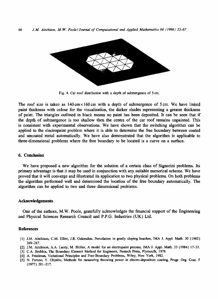
As an example we consider the paint distribution obtained on the roof of a car. Physically, the car body shells are attached to a large joist which lowers them into the bath containing the electrolyte solution. It is observed in practice that the depth of the solution above the car roof is critical in obtaining an even distribution over the whole roof. The effect of different submergence depths can only be modelled by utilizing a three-dimensional numerical algorithm. We model the car roof and the volume of electrolyte above it using a parallelopiped. We take the bottom face to be the car roof. This means that we are approximating the car roof by a flat rectangle. This is valid since the curvature of a typical car roof is slight, particularly towards the centre of the roof which is our primary area of interest. The top face is the surface of the electrolyte solution with insulating air above it (and so we take the boundary condition to be &$/an = 0 here). To simplify the computations, we do not directly model the bath but note the observations of Furuno and Ohyabu [5] that the potential drop from the anodes situated on the side of the bath to the workpiece is negligible. Instead we take the other four sides of the parallelopiped as forming a boundary to this area and take the anodic potential as applying at these four sides.

Since the primary area of interest is on the car roof we will again use the Boundary Element Method. All the surfaces which form the boundary of the three-dimensional region are divided into triangular elements on which we take piecewise constant approximations for 4 and 84/&z. Following the discussion in Section 4, the interface between the areas of coated and uncoated metal then lies along element edges.

Fig. 4 shows the effect of having a submergence depth which is too shallow. For this we used a value of E = 0.006 obtained from matching numerical results with experimental observations [ 131.

66 J.M. Aitchison, M. W. Poole/ Journal of Computational and Applied Mathematics 94 (1998) 55-47

Fig. 4. Car roof distribution with a depth of submergence of 5 cm.

The roof size is taken as 140 cmx 160 cm with a depth of submergence of 5 cm. We have linked paint thickness with colour for the visualisation, the darker shades representing a greater thickness of paint. The triangles outlined in black means no paint has been deposited. It can be seen that if the depth of submergence is too shallow then the centre of the car roof remains unpainted. This is consistent with experimental observations. We have shown that the switching algorithm can be applied to the electropaint problem where it is able to determine the free boundary between coated and uncoated metal automatically. We have also demonstrated that the algorithm is applicable to three-dimensional problems where the free boundary to be located is a curve on a surface.

6. Conclusion

We have proposed a new algorithm for the solution of a certain class of Signorini problems. Its primary advantage is that it may be used in conjunction with any suitable numerical scheme. We have proved that it will converge and illustrated its application to two physical problems. On both problems the algorithm performed well and determined the location of the free boundary automatically. The algorithm can be applied to two and three dimensional problems.

Acknowledgements

One of the authors, M.W. Poole, gratefully acknowledges the financial support of the Engineering and Physical Sciences Research Council and P.P.G. Industries (UK) Ltd.

References

Ill

I21 [31 141 PI

J.M. Aitchison, C.M. Elliot, J.R. Ockendon, Percolation in gently sloping beaches, IMA J. Appl. Math. 30 (1983) 269-287. J.M. Aitchison, A.A. Lacey, M. Shillor, A model for an electropaint process, IMA J. Appl. Math. 33 (1984) 17-31. C.A. Brebbia, The Boundary Element Method for Engineers, Pentech Press, Plymouth, 1978. A. Friedman, Variational Principles and Free-Boundary Problems, Wiley, New York, 1982. N. Furuno, Y. Ohyabu, Methods for measuring throwing power in electro-deposition coating, Progr. Org. Coat. 5 (1977) 201-217.

J.M. Aitchison, M. W. PoolelJoumal of Computational and Applied Mathematics 94 (1998) 5567 67

[6] R. Glowinski, Numerical Methods for Nonlinear Variational Problems, Springer, New York, 1982. [7] J. Haslinger, Signorini problem with Coulomb’s law of friction. Shape optimization in contact problems, Internat.

J. Numer. Methods Eng. 34 (1992) 223-23 1. [8] A. Karageorghis, Numerical solution of a shallow dam problem by a boundary element method, Comput. Methods

Appl. Mech. Eng. 61 (1987) 265-276. [9] F. Lebon, M. Raous, Multibody contact problem including friction in structure assembly, Comput. and Struct. 43

(1992) 925-934. [lo] J. Nedoma, Finite element analysis of contact problems in thermoelasticity. The semicoercive case, J. Comput. Appl.

Math. 50 (1994) 411-423. [1 l] P. Neittaamn&i, Design sensitivity analysis for state-constrained structural design problems, Mech. Struct. and Mach.

20 (1992) 433-458. [12] K. Petrov, N. Petrov, M. Mikrenska, A computer program for solving Signorini’s contact problem with friction, Adv.

Eng. Software 19 (1994) 97-108. [ 131 M.W. Poole, J.M. Aitchison, Numerical model of an electropaint process with applications to the automotive industry,

IMA J. Math. Appl. Bus. Ind. 8 (1997) 347-360. [14] M.H. Protter, H.F. Weinberger, Maximum Principles in Differential Equations, Springer, Berlin, 1984. [ 151 A. Signorini, Sopra alcune questioni di elastostatica, Atti della Societa per il Progress0 della Scienza (1993).