a numerical approach to the contract theory: the … numerical approach to the contract theory: the...
TRANSCRIPT

GRIPS Discussion Paper 11-27
A Numerical Approach to the Contract Theory:
the Case of Adverse Selection
Hideo Hashimoto
Kojun Hamada
Nobuhiro Hosoe
March 2012
National Graduate Institute for Policy Studies
7-22-1 Roppongi, Minato-ku,
Tokyo, Japan 106-8677

Page 1
A Numerical Approach to the Contract Theory: the Case
of Adverse Selection
Hideo Hashimoto*, Kojun Hamada†, Nobuhiro Hosoe‡
Abstract:
By building and solving numerical models of the parts supply problems (an
example of the adverse selection problems), and analyzing various issues of the contract
theory, we demonstrate the benefits of the numerical approach. First, this approach
facilitates the understanding of the contract theory by beginners, who find it difficult to
comprehend the theoretical and general models. Second, this approach could extend the
analysis areas beyond those of the theoretical models, which are limited by the simplifying
assumptions imposed in order to make their analysis possible. The expansion of the number
of the supplier types is one example.
Keywords:
Numerical approach; principal-agent problem; adverse selection; numerical and
computational model; Spence-Mirrlees single crossing property; monotonicity
* Professor Emeritus of Osaka University
† Faculty of Economics, Niigata University
‡ Corresponding author. National Graduate Institute for Policy Studies, 7-22-1 Roppongi, Minato,
Tokyo 106-8677. E-mail: [email protected].
GRIPS Policy Research Center Discussion Paper : 11-27

Page 2
1. A Numerical Approach
In this paper, we build and solve various numerical models of the “parts supply
problems” as an example of the adverse selection problems for the following two purposes.
First, the paper aims to facilitate beginners of the contract theory to understand it with the
numerical models. Since many earlier studies have developed the contract theory models in
a theoretical and general manner, the beginners often encounter difficulties of
understanding them. Second, we demonstrate some advantages of the numerical approach
over that theoretical approach. For example, we can easily assume a larger number of the
supplier’s types than two or three, which is often assumed in theoretical studies.
Furthermore, we can extend the analysis area that is limited by some simplifying
assumptions used in those theoretical studies. In addition by applying the Monte Carlo
simulation method, we can investigate the likelihood that those assumptions hold. To
understand the numerical models fully, the readers must know the computer programs,
which will be explained in details in the earlier part of this paper.
To analyze the parts supply problems, we formulate the models as non-linear
programming problems. Then, by specifying functional forms and feeding some numbers
into parameters, we build and solve the numerical computer models. In this numerical
approach, we obtain not only the optimal values of the primal variables, such as the parts
quality and the price to be paid to the supplier, but also the optimal values of the Lagrange
multipliers of the imposed constraints. The information rent, which is the most important
variable in problems with asymmetric information, can be derived directly from the solved
values of some Lagrange multipliers. Furthermore, we can easily conduct comparative
statics by changing the values of some parameters.
To build and solve the numerical models, we use GAMS (General Algebraic
GRIPS Policy Research Center Discussion Paper : 11-27

Page 3
Modeling System) as computation software.1 While in this paper we explain the essential
GAMS syntax, refer to Hosoe et al. (2010, Chapter 3) for more detailed explanation. The
readers can realize the contract theory well, by playing around with the models presented in
this paper, i.e., changing the values of some parameters in our sample programs with use of
the trial version of GAMS.
On one hand, of course, we must be careful in deriving any general conclusions
from numerical models which are based on specific functional forms and assumed
parameters. In addition, it is not an easy job to master a new computer language to deal
with numerical models freely. On the other hand, our approach to develop numerical models,
which depict the essence of the theoretical models, will afford the readers ease in
comprehending the contract theory. The authors hope the readers find the heuristic
usefulness in this paper.
This paper originates from our previous paper by Hashimoto et al. (2011) written in
Japanese where various numerical models of the parts supply problems are developed,
based on the theoretical models by Itoh (2003). We also use the analytical frameworks
demonstrated by Itoh (2003) when we develop our numerical examples.
2. Adverse Selection: the Parts Supply Problem
The parts supply problems are the basic problems of adverse selection. A maker (a
principal, called with a female pronoun), making a unit of a final product, purchases its
parts from a supplier (an agent, called with a male pronoun) for her production. There are
several technical types (efficient or inefficient, etc.) of the supplier. Only the supplier knows
about his type (i.e., private information). Under these circumstances, the maker is supposed
1 GAMS is commercial software; however, its trial version can be downloaded from the website of
GAMS Development Corporation (http://www.gams.com/dowmload/) and used without charge. The
numerical models presented in this paper are so small that they can be solved with the trial version.
GRIPS Policy Research Center Discussion Paper : 11-27

Page 4
to offer a contract that maximizes her utility.
The contract that the maker offers is the mechanism to determine the quality of
the parts ix to be produced by the i -th type supplier and the price iw to be paid to him,
in such a way as to maximize the maker’s utility, based on the supplier’s report about his
type. If, hypothetically, the maker knew the supplier’s type (symmetric information), there
were no possibility that the supplier would report his type falsely; thus, the first-best would
be realized. However, in reality, the maker does not know the supplier’s type (asymmetric
information) and, thus, must offer a contract in such a way as to make the supplier obtain no
extra gain, even if he should report his type falsely. Such a contract is the second-best
optimal in the sense that it minimizes the inefficiency resulted from asymmetric
information. As the maker must be compromised with the supplier exploiting his
asymmetric information, her second-best utility level is lower than the first-best one.
The supplier’s type in our models is a discrete variable. In Section 2.1, we consider
the cases with two supplier types (efficient and inefficient). We solve the first-best
equilibrium by assuming no asymmetric information as the benchmark case. Next, we
present the second-best model, where the (global) incentive compatibility conditions are
needed to prevent the supplier from reporting his type falsely. Subsequently, we consider the
cases with three supplier types in Sections 2.2 and 2.3. When the number of types increases–
from two to N in general, the incentive compatibility conditions become complicated.
Because the number of possible combinations that the i -th type supplier reports his type
truly or falsely as “type j” increases, that of incentive compatibility conditions to prevent his
false reporting increases rapidly. Additional assumptions–the Spence-Mirrlees single
crossing property (SCP) and monotonicity (MN)–are introduced to simplify these conditions.
(The SCP and monotonicity will be explained in details in Section 2.2.3.) These simplifying
assumptions make the analysis of the theoretical contract models possible.
In Section 2.2, we examine the simplest models with these two assumptions. In
Section 2.3, we extend the models in two directions. First, we increase the number of
GRIPS Policy Research Center Discussion Paper : 11-27

Page 5
supplier types. It can be done easily without complicated programming techniques. Second,
we deal with the models where these assumptions of the SCP and MN do not hold. This also
can be done without causing technical difficulties. Finally, in Section 2.4, applying the
Monte Carlo simulation method, we “estimate” the likelihood that such assumptions as the
SCP and MN hold, and discuss the importance of these assumptions in a contract theory
analysis.
2.1 The 2-type Models
We consider two supplier types (efficient and inefficient). In the former part of this
subsection, we develop the first-best models, where the maker knows the supplier’s type, i.e.,
his marginal cost of the parts production. For benefits of those unfamiliar to GAMS
computer models, we first present the model only with the efficient supplier; then, the one
only with the inefficient supplier separately. Next, we combine these two models into one
model that includes both types.
In the latter part, we present the second-best model, where the maker does not
know the supplier’s type. Then, we develop one model that includes both the first-best and
the second-best. Finally, we compare the second-best solutions with the first-best solutions.
2.1.1 The First-best Model with Only One Supplier Type
The first-best model (or, the benchmark model) of the parts supply problem is for
the maker to offer a contract that determines the parts quality ix to be produced by the
supplier and the price iw to be paid to him, knowing the supplier’s marginal cost i ,
theta(i). In the first, we build a model of the case that the maker knows the supplier is
efficient, and in the second a model of the case that the maker knows the supplier is
inefficient. These models are built separately. The models are to simply maximize the
maker’s utility under non-negativity constraints on the decision variable ix .
GRIPS Policy Research Center Discussion Paper : 11-27

Page 6
2.1.2 The Fist-Best Model with the Efficient Supplier (PS2_F_eff.gms)2
Let us go through the input file of the first-best model with the efficient supplier
(List 2.1). The first-best model when the supplier type is known to be efficient is expressed
as the following maker's utility maximization problem:
i
iii xcxbUtilmax (2.1)
subject to
5.0ii xxb i (2.2)
0 iiii xxc i (2.3)
List 2.1: The First-best Model with the Efficient Supplier (PS2_F_eff.gms) ...
7 * Definition of Set 8 Set i type of supplier /eff/; 9 * Definition of Parameters 10 Parameter 11 theta(i) efficiency /eff 0.2/; 12 * Definition of Primal/Dual Variables 13 Positive Variable 14 x(i) quality 15 b(i) maker's revenue 16 c(i) cost; 17 Variable 18 Util maker's utility; 19 Equation 20 obj maker's utility function 21 rev(i) maker's revenue function 22 pc(i) participation constraint; 23 * Specification of Equations 24 obj.. Util =e= sum(i, (b(i)-c(i))); 25 rev(i)..b(i) =e= x(i)**(0.5); 26 pc(i).. c(i)-theta(i)*x(i) =e= 0; 27
2 Those in the parentheses after the section titles show GAMS input file names shown in the following
part.
GRIPS Policy Research Center Discussion Paper : 11-27

Page 7
28 * Setting Lower Bounds on Variables to Avoid Division by Zero 29 x.lo(i)=0.0001;; 30 31 * Defining and Solving the Model 32 Model FB1 /all/; 33 Solve FB1 maximizing Util using NLP; 34 35 Parameter 36 db(i) derivative of b 37 w(i) price 38 ; 39 db(i) =0.5*x.l(i)**(-0.5); 40 w(i) =c.l(i); 41 42 Display x.l, b.l, c.l, util.l, db, w; 43 * End of Model
In Line 8, the supplier’s type is expressed right after the Set directive as an index
i (i.e., the suffix i in ordinary algebraic equations), such as i =eff (the efficient supplier)
and i =inf (the inefficient supplier). As this model has only the efficient supplier, the index
i can be omitted. However, the index i is kept because the same model is used later as the
model with an inefficient supplier by replacing eff with inf. The efficiency of each supplier
type, denoted by his marginal cost of the parts theta(i) ( i in the mathematical model) is
shown in Line 11.
In Lines 13–18, the decision (endogenous) variables are declared. The decision
variables are the quality of supplier i ’s parts x(i), the maker’s revenue received from
supplier i ’s parts b(i), and supplier i ’s cost c(i). And, as these variables must be
non-negative, they are declared with the Positive Variable directive. 3 The other
endogenous variable is the value of the objective function, whose name is defined as Util.
As the sign of the value of Util is not known before solving the model, it must be declared
with the Variable directive so that its value can be either positive or negative. Lines 19–22
show the names of the objective function (i.e., the maker’s utility function) and the
3 In GAMS, Positive Variable means non-negative variable; thus, it can be zero.
GRIPS Policy Research Center Discussion Paper : 11-27

Page 8
constraints or the equations (i.e., revenue function and cost function). In GAMS programs,
names must be given to all equations (including the objective function).4 The names of the
objective function (2.1), revenue function (2.2), and cost function (2.3) are named as obj,
rev(i), and pc(i)in the program, respectively.
Lines 24–26 define the equations (including the objective function), which
constitute the maximization problem presented above. Line 24 shows the objective function.5
Line 25 expresses the maker’s revenue b , which is assumed to be a simple concave
function 5.0ii xxb . Line 26 shows the supplier’s cost ic as a linear function of ix
with the constant marginal cost i . In GAMS, “=e=” means strict equality, “*”(unless it
appears in the first column in a line) is multiplication, and “**” means power.
In Line 29, an arbitrary very small positive value is assigned as the lower bound of
x(i) so as to avoid computational problems (e.g., division by zero). If a solution matches this
lower bound, we must reconsider the lower bound, because this solution may be affected by
this artificially-set lower bound. Line 32 gives the model name FB1 to the model consisting
of all the equations including the objective function. Line 33 is a statement to solve the
model FB1 maximizing Util by using a non-linear programming problem (NLP) solver.
The lines after Line 34 are added for further analyses. The symbol db(i) means
the value of the first-order derivative of b(i) with respect to x(i) evaluated at the solution
of x(i). Although the contract must include not only the parts quality x(i) but also the
4 While we often use mechanical equation names, such as Equation 1, Equation 2, etc. in
mathematical expressions, we can freely make names that suggest the meanings of the equations in
GAMS.
5 The objective function is the weighted sum of the difference between revenues and costs for all i .
The sum in algebraic equations ...i is expressed as “sum(i, …)” in GAMS. The summation,
however, does not carry any significance here because we consider only one supplier type for i .
GRIPS Policy Research Center Discussion Paper : 11-27
price
maxi
being
has t
(Whe
“x.l(
solve
Whil
ordin
Disp
multi
maxi
unde
(As t
stron
GAM
the in
the n
in th
List 2 ...
6 As f
(2010
e w(i) to b
imization pr
g simply equ
the full barg
en the solved
(i)”. Note t
ed values of t
e the equali
nary equality
play statem
ipliers and t
Finally,
imization or
erstand the m
ime passes,
ngly recomm
When y
MS IDE, click
nput file an
numbers in t
e input file.
2.2: Output (PS2_F_
for GAMS an
0), and McCar
be paid to t
roblem speci
uated to c(i
gaining powe
d values are
that “l” in th
the Lagrang
ty symbol “=
y symbol “=
ment in Line
the compute
lines start
r any compu
model conten
the modele
mended to wr
you make a
k the o
d generates
the furtherm
Those numb
File for the _eff.lst)
nd GAMS IDE
rl (2009).
the i -th typ
ified above.
), following
er at the tim
e used for com
he suffix is n
ge multiplier
=e=” is used
=” is used for
e 42 is to p
ed values of t
ing with “*”
utation. The
nts but also
rs themselv
rite as much
a computer
on the menu
the output
most left colu
bers should
First-best M
E, refer to Ho
pe supplier
Thus, the v
the “take-it
me of the con
mputation, “
not a numer
rs of constra
d for equation
r equations
print the sol
the equation
” (asterisk)
ese memos n
could help t
ves often can
h detailed me
program st
u bar; then,
file.6 The ou
umn are put
not be put i
Model for th
osoe et al. (20
, the latter
value of w(i
t-or-leave-it
ntract negoti
“.l” is attac
ral “1” but a
aints, “.m” is
ns within th
outside the
lutions inclu
ns specified
are simply
not only wou
the modelers
nnot recall w
emos as pos
tated above
GAMS com
utput file is
only for exp
in the input
e Efficient S
010, Chapter
is not to b
i) is comput
offer” assum
iation in the
ched to the v
Roman lette
attached as
he maximiza
e maximizat
uding those
in the lines
memos, wh
uld facilitat
s recall their
what they ha
sible.
by using a
mputes the m
shown in L
planation an
file, when y
Supplier
3 and Appen
be shown i
ted in Line
mption–the m
e first-best m
variables, su
er “el”. To u
s, say, “pc.m
ation problem
tion problem
of the Lag
after Line 3
hich do not
te other peo
r thought pr
ave written.
a software
models writt
List 2.2. Note
nd are the sa
you write it.
ndix C), Brook
Page 9
n the
40 by
maker
model.
uch as
se the
m(i)”.
m, the
m. The
grange
34.
affect
ple to
ocess.
.) It is
called
ten in
e that
me as
k et al.
GRIPS Policy Research Center Discussion Paper : 11-27

Page 10
2 7 * Definition of Set 3 8 Set i type of supplier /eff/; 4 9 * Definition of Parameters 5 10 Parameter 6 11 theta(i) efficiency /eff 0.2/; 7 12 * Definition of Primal/Dual Variables 8 13 Positive Variable 9 14 x(i) quality
... 11 S O L V E S U M M A R Y 12 13 MODEL FB1 OBJECTIVE Util 14 TYPE NLP DIRECTION MAXIMIZE 15 SOLVER CONOPT FROM LINE 33 16 17 **** SOLVER STATUS 1 NORMAL COMPLETION 18 **** MODEL STATUS 2 LOCALLY OPTIMAL 19 **** OBJECTIVE VALUE 1.2500
... 21 ** Optimal solution. Reduced gradient less than tolerance.
... 23 LOWER LEVEL UPPER MARGINAL 24 25 ---- EQU obj . . . 1.000 26 27 obj total surplus function 28 29 ---- EQU rev maker's revenue function 30 31 LOWER LEVEL UPPER MARGINAL 32 33 eff . . . 1.000 34 35 ---- EQU pc participation constraint 36 37 LOWER LEVEL UPPER MARGINAL 38 39 eff . . . -1.000 40 41 ---- VAR x quality 42 43 LOWER LEVEL UPPER MARGINAL 44 45 eff 1.0000E-7 6.250 +INF EPS 46 47 ---- VAR b maker's revenue 48 49 LOWER LEVEL UPPER MARGINAL
GRIPS Policy Research Center Discussion Paper : 11-27

Page 11
50 51 eff . 2.500 +INF . 52 53 ---- VAR c cost 54 55 LOWER LEVEL UPPER MARGINAL 56 57 eff . 1.250 +INF . 58 59 LOWER LEVEL UPPER MARGINAL 60 61 ---- VAR Util -INF 1.250 +INF .
... 63 ---- 42 VARIABLE x.L quality 64 65 eff 6.250 66 67 68 ---- 42 VARIABLE b.L maker's revenue 69 70 eff 2.500 71 72 73 ---- 42 VARIABLE c.L cost 74 75 eff 1.250 76 77 78 ---- 42 VARIABLE Util.L = 1.250 total surplus79 80 ---- 42 PARAMETER db derivative of b 81 82 eff 0.200 83 84 85 ---- 42 PARAMETER w price 86 87 eff 1.250
...
In the first part of the output file, the codes originally put in the input file appear
with their line numbers (i.e., echo print). Make sure that “**optimal solution” appears
in the SOLVE SUMMARY part after this echo print as shown in Line 21 of List 2.2. (If not,
whatever results are meaningless as solutions.) Then, there are two types of solutions; EQU
GRIPS Policy Research Center Discussion Paper : 11-27
Page 12
(mainly, expressing the Lagrange multipliers of the constraints) and VAR (mainly, the solved
values of the decision or endogenous variables). The EQU block comes first. In the EQU block,
the Lagrange multipliers are shown in the column under MARGINAL.7 For example, the
Lagrange multiplier of constraint rev(i) is 1.000. (Incidentally, in any maximization
problem, the Lagrange multiplier of the objective function is always unity.)
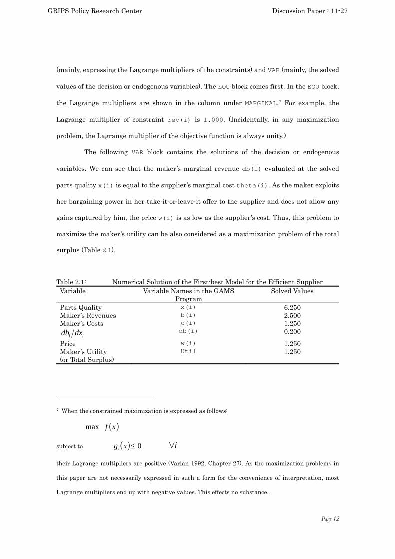
The following VAR block contains the solutions of the decision or endogenous
variables. We can see that the maker’s marginal revenue db(i) evaluated at the solved
parts quality x(i) is equal to the supplier’s marginal cost theta(i). As the maker exploits
her bargaining power in her take-it-or-leave-it offer to the supplier and does not allow any
gains captured by him, the price w(i) is as low as the supplier’s cost. Thus, this problem to
maximize the maker’s utility can be also considered as a maximization problem of the total
surplus (Table 2.1).
Table 2.1: Numerical Solution of the First-best Model for the Efficient Supplier Variable Variable Names in the GAMS
Program Solved Values
Parts Quality x(i) 6.250 Maker’s Revenues b(i) 2.500 Maker’s Costs c(i) 1.250
ii dxdb db(i) 0.200
Price w(i) 1.250 Maker’s Utility (or Total Surplus)
Util 1.250
7 When the constrained maximization is expressed as follows:
xfmax
subject to 0xgi i
their Lagrange multipliers are positive (Varian 1992, Chapter 27). As the maximization problems in
this paper are not necessarily expressed in such a form for the convenience of interpretation, most
Lagrange multipliers end up with negative values. This effects no substance.
GRIPS Policy Research Center Discussion Paper : 11-27

Page 13
2.1.3 The First-best Model with the Inefficient Supplier (PS2_F_inf.gms)
The first-best model with the inefficient supplier can be built by making the
following two changes in the original input file of PS2_F_eff.gms:
in Line 8, replace eff appearing as the element of set i by inf
in Line 11, put the marginal cost of the inefficient supplier for theta(i)
The solutions of the maximization problem and the values computed from the
solutions are in Table 2.2. As pointed out in Section 2.1.2, the maker’s marginal revenue
db(i) evaluated at the solved parts quality x(i) is equal to the supplier’s marginal cost
theta(i), and this utility maximization coincides with the maximization of the total
surplus.
Table 2.2: Numerical Solution of the First-best Model for an Inefficient Supplier Variable Variable Names in the GAMS
Program Solved Values
Parts Quality x(i) 2.778 Maker’s Revenues b(i) 1.667 Maker’s Costs c(i) 0.833
ii dxdb db(i) 0.300
Price w(i) 0.833 Maker’s Utility (or Total Surplus)
Util 0.833
2.1.4 The First-Best Model with Both Supplier Types (PS2_F.gms)
Now that we deal with a model that includes both supplier types, we introduce an
ex-ante probability ip which indicates the i -th type exists. We assume that the maker
knows this probability (common knowledge). The maximization problem of the first-best
model is written in the following:
i
iii wxbpUtilmax (2.1’)
subject to
GRIPS Policy Research Center Discussion Paper : 11-27

Page 14
5.0ii xxb i (2.2)
ruxw iii i (2.3’)
In comparison with the maximization problem consisting of (1.1)-(1.3), there are two
changes made. The first change is made in the objective function (2.1’). Now, the maker’s
utility weighted with the probability is maximized. The second change is made in (2.3’). In
the previous model, by assuming the take-it-or-leave-it offer on an a priori basis, no surplus
is given to the supplier; thus, ic is solved first. Then, ic is equated to iw . In the present
model, we explicitly use iw as a decision variable. Then, we introduce the participation
constraint that the supplier’s (net) utility, i.e., his receipt from the maker w(i) minus the
production cost theta(i)*x(i), must be greater than or equal to the reservation utility
ru–the minimum utility with which the supplier participates in the contract. If this
condition is not satisfied, the supplier does not accept the contract offered by the maker.
The explanation on the input file of the computer model in the following will be
centered on the differences from the previous models (List 2.3). In Line 8, both supplier
types eff and inf are put as the elements of Set i. In Lines 11–16, the marginal costs
theta(i) and the probability p(i) of both supplier types are put. In Line 17, the
reservation utility ru is given. Although ru is set to be zero in this numerical example, it can
be any number.
In Lines 20–25, the decision variables are defined. Differently from the previous
models, w(i) is defined as a decision variable in this model. In Lines 26–29, the names of
the objective functions and the equations are shown. Lines 32–34 contain the equations of
the maximization problem. Line 32 shows the objective function. The maker’s utility is the
sum of net revenues (i.e., the profit margin between b(i) and w(i)) weighted with the
probability. Line 33 is the revenue function, defined as 5.0
ii xb as in the previous models.
Line 34 represents the participation constraint. The inequality symbol is expressed as
“=g=” in GAMS programs. Line 40 defines the model that consists of all the equations, and
GRIPS Policy Research Center Discussion Paper : 11-27

Page 15
Line 41 is a directive to solve the model by maximizing the maker’s utility Util.
List 2.3: The Integrated First-best Model for Two Supplier Types (PS2_F.gms) ...
7 * Definition of Set 8 Set i type of supplier /eff, inf/; 9 10 * Definition of Parameters 11 Parameter 12 theta(i) efficiency /eff 0.2 13 inf 0.3/ 14 prob(i) probability of type 15 /eff 0.2 16 inf 0.8/; 17 Scalar ru reservation utility /0/; 18 19 * Definition of Primal/Dual Variables 20 Positive Variable 21 x(i) quality 22 b(i) maker's revenue 23 w(i) price; 24 Variable 25 Util total surplus; 26 Equation 27 obj supplier's profit function 28 rev(i) maker's revenue function 29 pc(i) participation constraint; 30 31 * Specification of Equations 32 obj.. Util =e= sum(i, prob(i)*(b(i)-w(i))); 33 rev(i)..b(i) =e= x(i)**(0.5); 34 pc(i).. w(i)-theta(i)*x(i) =e= 0; 35 36 * Setting Lower Bounds on Variables to Avoid Division by Zero 37 x.lo(i)=0.0000001; 38 39 * Defining and Solving the Model 40 model FB1 /all/; 41 solve FB1 maximizing Util using NLP; 42 43 * End of Model
The Lagrange multipliers of the participation constraints pc(i) are binding for both
supplier types (Lines 128-133, of List 2.4). This means that the maker, who knows the
GRIPS Policy Research Center Discussion Paper : 11-27

Page 16
supplier type, offers him the price, depending upon his type, with which his utility is
indifferent from the reservation level ru. The solved values of the parts quality x(i), the
maker’s revenue b(i), and the maker’s utility Util are shown in the VAR block.
List 2.4: Output File of the Integrated First-best Model (PS2_F.lst) 74 S O L V E S U M M A R Y 75 76 MODEL FB1 OBJECTIVE Util 77 TYPE NLP DIRECTION MAXIMIZE 78 SOLVER CONOPT FROM LINE 41 79 80 **** SOLVER STATUS 1 NORMAL COMPLETION 81 **** MODEL STATUS 2 LOCALLY OPTIMAL 82 **** OBJECTIVE VALUE 0.9167 ... 117 ---- EQU obj . . . 1.000 118 119 obj supplier's profit function 120 121 ---- EQU rev maker's revenue function 122 123 LOWER LEVEL UPPER MARGINAL 124 125 eff . . . 0.200 126 inf . . . 0.800 127 128 ---- EQU pc participation constraint 129 130 LOWER LEVEL UPPER MARGINAL 131 132 eff . . . -0.200 133 inf . . . -0.800 134 135 ---- VAR x quality 136 137 LOWER LEVEL UPPER MARGINAL 138 139 eff 1.0000E-7 6.250 +INF 2.0951E-9 140 inf 1.0000E-7 2.778 +INF EPS 141 142 ---- VAR b maker's revenue 143 144 LOWER LEVEL UPPER MARGINAL 145 146 eff . 2.500 +INF .
GRIPS Policy Research Center Discussion Paper : 11-27
Page 17
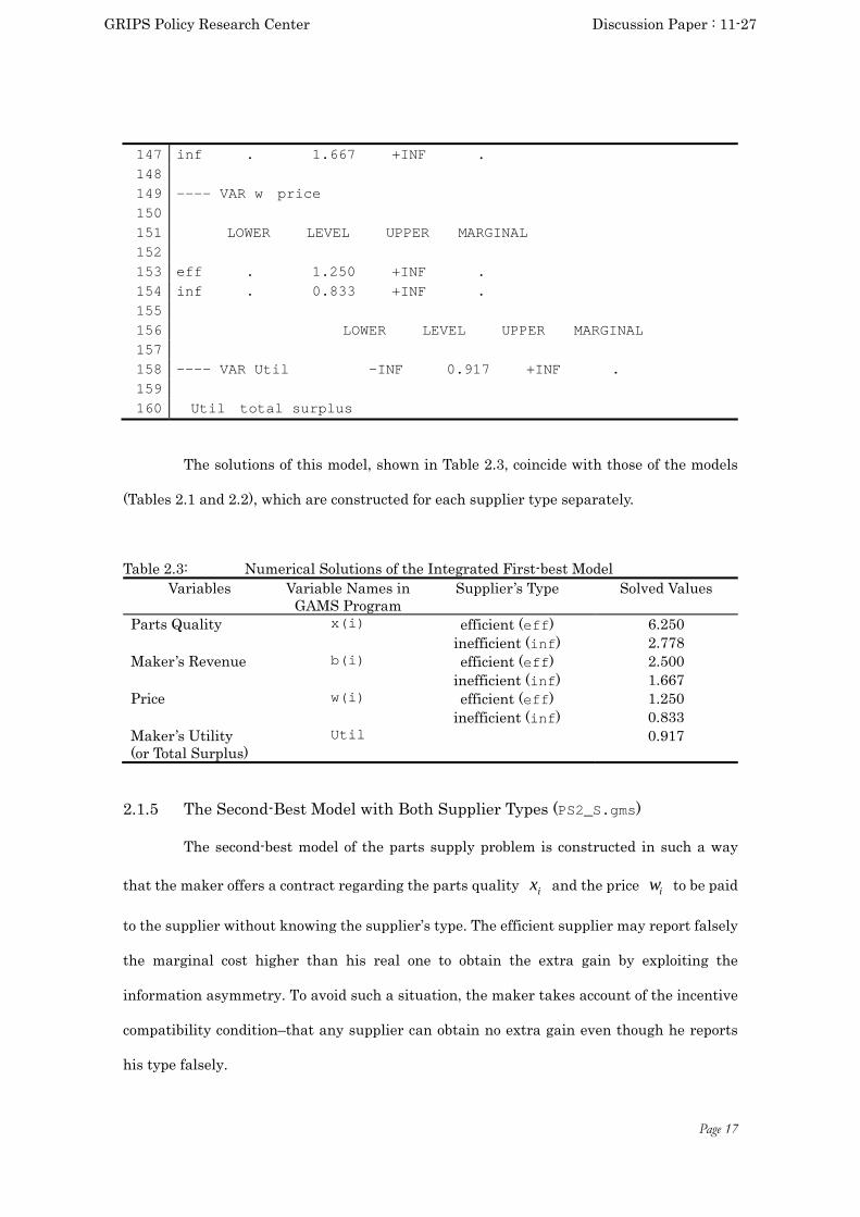
147 inf . 1.667 +INF . 148 149 ---- VAR w price 150 151 LOWER LEVEL UPPER MARGINAL 152 153 eff . 1.250 +INF . 154 inf . 0.833 +INF . 155 156 LOWER LEVEL UPPER MARGINAL 157 158 ---- VAR Util -INF 0.917 +INF . 159 160 Util total surplus
The solutions of this model, shown in Table 2.3, coincide with those of the models
(Tables 2.1 and 2.2), which are constructed for each supplier type separately.
Table 2.3: Numerical Solutions of the Integrated First-best Model Variables Variable Names in
GAMS Program Supplier’s Type Solved Values
Parts Quality x(i) efficient (eff) 6.250 inefficient (inf) 2.778 Maker’s Revenue b(i) efficient (eff) 2.500 inefficient (inf) 1.667 Price w(i) efficient (eff) 1.250
inefficient (inf) 0.833 Maker’s Utility (or Total Surplus)
Util 0.917
2.1.5 The Second-Best Model with Both Supplier Types (PS2_S.gms)
The second-best model of the parts supply problem is constructed in such a way
that the maker offers a contract regarding the parts quality ix and the price iw to be paid
to the supplier without knowing the supplier’s type. The efficient supplier may report falsely
the marginal cost higher than his real one to obtain the extra gain by exploiting the
information asymmetry. To avoid such a situation, the maker takes account of the incentive
compatibility condition–that any supplier can obtain no extra gain even though he reports
his type falsely.
GRIPS Policy Research Center Discussion Paper : 11-27
Page 18
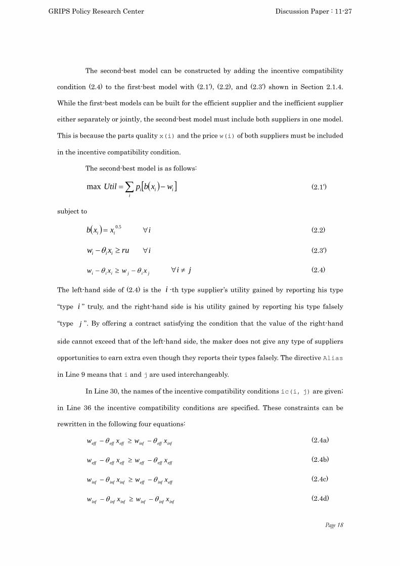
The second-best model can be constructed by adding the incentive compatibility
condition (2.4) to the first-best model with (2.1’), (2.2), and (2.3’) shown in Section 2.1.4.
While the first-best models can be built for the efficient supplier and the inefficient supplier
either separately or jointly, the second-best model must include both suppliers in one model.
This is because the parts quality x(i) and the price w(i) of both suppliers must be included
in the incentive compatibility condition.
The second-best model is as follows:
i
iii wxbpUtilmax (2.1’)
subject to
5.0ii xxb i (2.2)
ruxw iii i (2.3’)
jijiii xwxw ji (2.4)
The left-hand side of (2.4) is the i -th type supplier’s utility gained by reporting his type
“type i ” truly, and the right-hand side is his utility gained by reporting his type falsely
“type j ”. By offering a contract satisfying the condition that the value of the right-hand
side cannot exceed that of the left-hand side, the maker does not give any type of suppliers
opportunities to earn extra even though they reports their types falsely. The directive Alias
in Line 9 means that i and j are used interchangeably.
In Line 30, the names of the incentive compatibility conditions ic(i, j) are given;
in Line 36 the incentive compatibility conditions are specified. These constraints can be
rewritten in the following four equations:
infeffinfeffeffeff xwxw (2.4a)
effeffeffeffeffeff xwxw (2.4b)
effinfeffinfinfinf xwxw (2.4c)
infinfinfinfinfinf xwxw (2.4d)
GRIPS Policy Research Center Discussion Paper : 11-27

Page 19
The new model system includes the above four equations, compared with two equations of
the original system (2.4).8 Equations (2.4b) and (2.4d) trivially holds with strict equality and,
thus, are redundant in light of the original constraint (2.4). Consequently, there is no
difference between the system stated above and the original system of (2.4).
List 2.5: Input File of the Second-best Model (PS2_S.gms) ...
7 * Definition of Set 8 Set i type of supplier /eff, inf/; 9 Alias (i,j); 10 * Definition of Parameters 11 Parameter 12 theta(i) efficiency /eff 0.2 13 inf 0.3/ 14 prob(i) probability of type 15 /eff 0.2 16 inf 0.8/; 17 Scalar ru reservation utility /0/; 18 19 * Definition of Primal/Dual Variables 20 Positive Variable 21 x(i) quality 22 b(i) maker's revenue 23 w(i) price; 24 Variable 25 Util maker's utility; 26 Equation 27 obj total surplus function 28 rev(i) maker's revenue function 29 pc(i) participation constraint 30 ic(i,j) incentive compatibility constraint; 31 32 * Specification of Equations 33 obj.. Util =e= sum(i, prob(i)*(b(i)-w(i))); 34 rev(i)..b(i) =e= x(i)**(0.5); 35 pc(i).. w(i)-theta(i)*x(i) =g= ru;
8 If you feel uneasy with this redundancy, you can rewrite Line 36 as:
ic(i,j)$(ord(i) ne ord(j))..w(i)-theta(i)*x(i) =g= w(j)-theta(i)*x(j);
where “$(…)” means a dummy variable expressing a condition that the relation inside the parenthesis
holds. And, ”ord(i)” means the order of index i in the defined set, and “ne” means “not equal.”
GRIPS Policy Research Center Discussion Paper : 11-27

Page 20
36 ic(i,j)..w(i)-theta(i)*x(i) =g= w(j)-theta(i)*x(j); 37 38 * Setting Lower Bounds on Variables to Avoid Division by Zero 39 x.lo(i)=0.0000001; 40 41 * Defining and Solving the Model 42 model SB1 /all/; 43 solve SB1 maximizing Util using NLP; 44 45 * End of Model
The input file is shown in List 2.5: its solution is printed in the output file (List
2.6).
List 2.6: Output File of the Second-best Model (PS2_S.lst) ... 123 ---- EQU rev maker's revenue function 124 125 LOWER LEVEL UPPER MARGINAL 126 127 eff . . . 0.200 128 inf . . . 0.800 129 130 ---- EQU pc participation constraint 131 132 LOWER LEVEL UPPER MARGINAL 133 134 eff . 0.237 +INF . 135 inf . . +INF -1.000 136 137 ---- EQU ic incentive compatibility constraint 138 139 LOWER LEVEL UPPER MARGINAL 140 141 eff.inf . . +INF -0.200 142 inf.eff . 0.388 +INF EPS 143 144 ---- VAR x quality 145 146 LOWER LEVEL UPPER MARGINAL 147 148 eff 1.0000E-7 6.250 +INF 6.7551E-8 149 inf 1.0000E-7 2.367 +INF . 150 151 ---- VAR b maker's revenue
GRIPS Policy Research Center Discussion Paper : 11-27

Page 21
152 153 LOWER LEVEL UPPER MARGINAL 154 155 eff . 2.500 +INF . 156 inf . 1.538 +INF . 157 158 ---- VAR w price 159 160 LOWER LEVEL UPPER MARGINAL 161 162 eff . 1.487 +INF . 163 inf . 0.710 +INF . 164 165 LOWER LEVEL UPPER MARGINAL 166 167 ---- VAR Util -INF 0.865 +INF . ...
2.1.6 The First-Best and the Second-Best Integrated Models (PS2_F&S.gms)
In the previous sections, we built and solved the first-best and second-best models
individually. Now we present a program to solve both models as one model. Note that the
difference between both the first-best and second-best models is found only in the use of the
incentive compatibility conditions. The codes up to Line 39 in the new model (List 2.7) are
identical to those in the second-best model (List 2.5). Line 42 defines the first-best model as
FB1, which consists of three equations, obj, rev(i), and pc(i), and Line 43 directs the
computer to solve the model FB1 by maximizing Util. Similarly, Line 45 defines the
second-best model as SB1, which consists of four equations, obj, rev(i), pc(i), and
ic(i,j). The equation ic(i,j) is the incentive compatibility conditions. Line 46 directs
to solve the model SB1 by maximizing Util.
There are two technical points in the programming. First, in the previous models,
when we define the model, we include “all” the equations described in the preceding lines;
so we express the model contents as:
Model model-name /all/; Alternatively, we can express more explicitly like:
GRIPS Policy Research Center Discussion Paper : 11-27

Page 22
Model model-name /obj, rev, pc/; In other words, inside of “/…/”, we exactly place the equation names used for the model.
Note that the indices such as “(i)” are not used in “/…/”.
List 2.7: The First-best and the Second-best Integrated Model (PS2_F&S.gms) ...
7 * Definition of Set 8 Set i type of supplier /eff, inf/; 9 Alias (i,j); 10 * Definition of Parameters 11 Parameter 12 theta(i) efficiency /eff 0.2 13 inf 0.3/ 14 p(i) probability of type 15 /eff 0.2 16 inf 0.8/; 17 Scalar ru reservation utility /0/; 18 19 * Definition of Primal/Dual Variables 20 Positive Variable 21 x(i) quality 22 b(i) maker's revenue 23 w(i) price; 24 Variable 25 Util maker's utility; 26 Equation 27 obj maker’s utility function 28 rev(i) maker's revenue function 29 pc(i) participation constraint 30 ic(i,j) incentive compatibility constraint; 31 32 * Specification of Equations 33 obj.. Util =e= sum(i, p(i)*(b(i)-w(i))); 34 rev(i)..b(i) =e= x(i)**(0.5); 35 pc(i).. w(i)-theta(i)*x(i) =g= ru; 36 ic(i,j)..w(i)-theta(i)*x(i) =g= w(j)-theta(i)*x(j); 37 38 * Setting Lower Bounds on Variables to Avoid Division by Zero 39 x.lo(i)=0.0001;; 40 41 * Defining and Solving the Model 42 Model FB1 /obj,rev,pc/; 43 Solve FB1 maximizing Util using NLP; 44 45 Model SB1 /obj,rev,pc,ic/;
GRIPS Policy Research Center Discussion Paper : 11-27

Page 23
46 Solve SB1 maximizing Util using NLP; 47 48 * End of Model
Second, as we now solve multiple models in one computer program using the Solve
directive for several times, the same number of SOLVE SUMMARY’s appear in the output file.
At the top of each of SOLVE SUMMARY, the model name such as FB1 appears in Line 81 and
SB1 in Line 197 (List 2.8). You will find the output files of this new model encompassing the
solutions of the first-best and the second-best models.
List 2.8: Output File of the First-best and the Second-best Integrated Model (PS2_F&S.lst) ... 79 S O L V E S U M M A R Y 80 81 MODEL FB1 OBJECTIVE Util 82 TYPE NLP DIRECTION MAXIMIZE 83 SOLVER CONOPT FROM LINE 43 84 85 **** SOLVER STATUS 1 NORMAL COMPLETION 86 **** MODEL STATUS 2 LOCALLY OPTIMAL 87 **** OBJECTIVE VALUE 0.9167
... 195 S O L V E S U M M A R Y 196 197 MODEL SB1 OBJECTIVE Util 198 TYPE NLP DIRECTION MAXIMIZE 199 SOLVER CONOPT FROM LINE 46 200 201 **** SOLVER STATUS 1 NORMAL COMPLETION 202 **** MODEL STATUS 2 LOCALLY OPTIMAL 203 **** OBJECTIVE VALUE 0.8654 ...
2.1.7 Comparison of the Solutions between the First-best and the Second-best
Models
The comparison of the solutions between the first-best and the second-best models
are summarized in Table 2.4. The incentive compatibility condition is binding only for the
efficient supplier (i.e., the Lagrange multiplier for the efficient supplier is non-zero). In other
GRIPS Policy Research Center Discussion Paper : 11-27
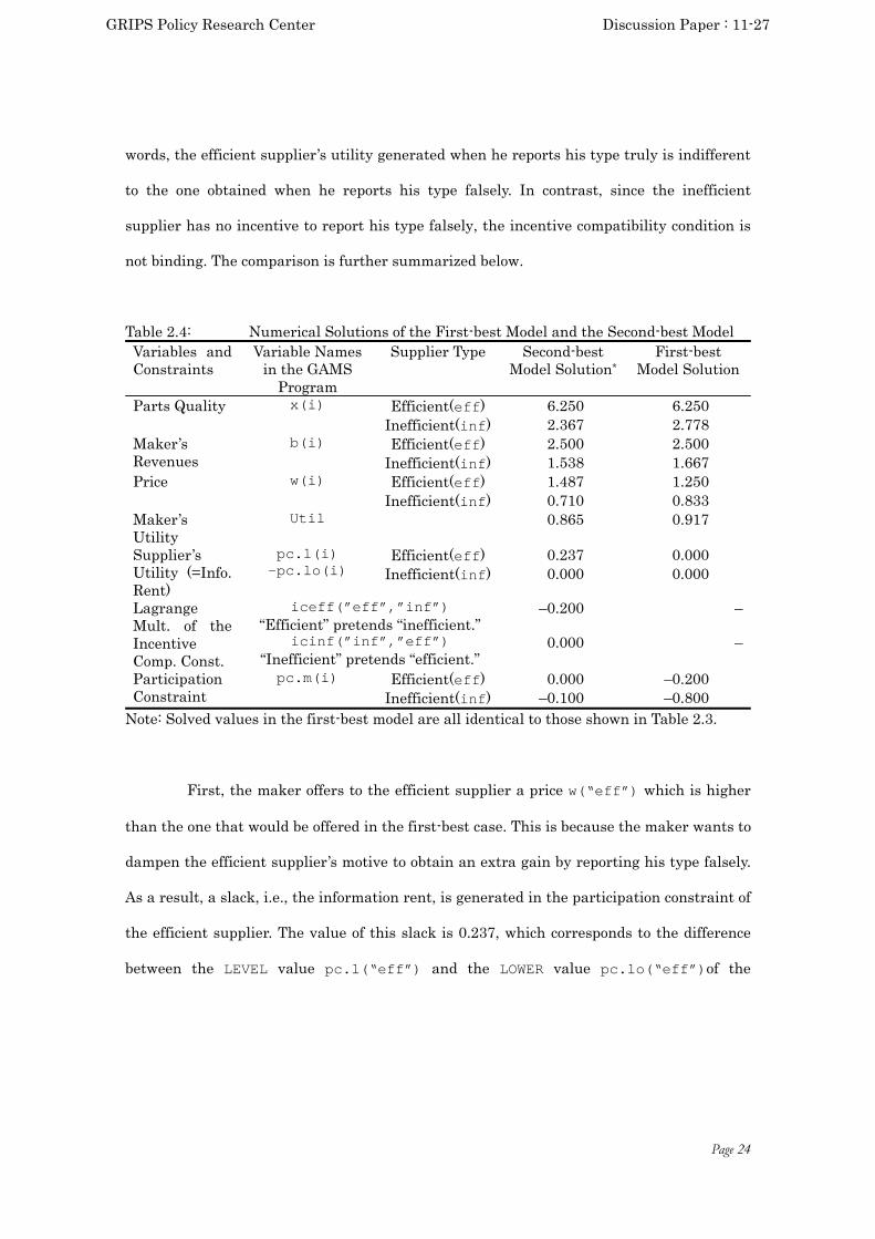
Page 24
words, the efficient supplier’s utility generated when he reports his type truly is indifferent
to the one obtained when he reports his type falsely. In contrast, since the inefficient
supplier has no incentive to report his type falsely, the incentive compatibility condition is
not binding. The comparison is further summarized below.
Table 2.4: Numerical Solutions of the First-best Model and the Second-best Model Variables and Constraints
Variable Names in the GAMS
Program
Supplier Type Second-best Model Solution*
First-best Model Solution
Parts Quality x(i) Efficient(eff) 6.250 6.250 Inefficient(inf) 2.367 2.778 Maker’s Revenues
b(i) Efficient(eff) 2.500 2.500 Inefficient(inf) 1.538 1.667
Price w(i) Efficient(eff) 1.487 1.250 Inefficient(inf) 0.710 0.833
Maker’s Utility
Util 0.865 0.917
Supplier’s Utility (=Info. Rent)
pc.l(i) -pc.lo(i)
Efficient(eff) 0.237 0.000 Inefficient(inf) 0.000 0.000
Lagrange Mult. of the Incentive Comp. Const.
iceff(”eff”,”inf”) “Efficient” pretends “inefficient.”
–0.200 –
icinf(”inf”,”eff”) “Inefficient” pretends “efficient.”
0.000 –
Participation Constraint
pc.m(i) Efficient(eff) 0.000 –0.200 Inefficient(inf) –0.100 –0.800
Note: Solved values in the first-best model are all identical to those shown in Table 2.3.
First, the maker offers to the efficient supplier a price w(“eff”) which is higher
than the one that would be offered in the first-best case. This is because the maker wants to
dampen the efficient supplier’s motive to obtain an extra gain by reporting his type falsely.
As a result, a slack, i.e., the information rent, is generated in the participation constraint of
the efficient supplier. The value of this slack is 0.237, which corresponds to the difference
between the LEVEL value pc.l(“eff”) and the LOWER value pc.lo(“eff”)of the
GRIPS Policy Research Center Discussion Paper : 11-27

Page 25
pc(“eff”).9 Because the reservation utility ru is assumed to be zero in the present model,
the information rent matches the efficient supplier’s utility. Even though the efficient
supplier enjoys a higher price, his parts quality remains as the same level in the first-best
case. His higher price results solely from his information rent.
Second, while in the second-best case the efficient supplier earns the information
rent, the maker does not allow the inefficient supplier to earn any information rent. The
maker offers the inefficient supplier a price w(“inf”), which is lower than the one in the
first-best case, in order not to make the efficient supplier’s information rent too liberal. As a
result, the inefficient supplier ends up with the lower quality. Third, the maker’s utility
decreases partly because of the information rent (0.237), which the maker must pay to the
efficient supplier and partly because of the loss resulted from the degraded parts quality
(0.411) made by the inefficient supplier.
2.2 The 3-Type Models
2.2.1 Outline of the 3-Type Models
In this section, we present the models distinguishing three supplier types (0, 1, 2;
the smaller number indicates the higher efficiency). The key difference of the N-type
( 3N ) models from the 2-type models lies in the complexity regarding the incentive
compatibility conditions of the second-best models. The 2-type models need incentive
compatibility conditions to prevent a false-reporting only for two cases. The one is the case
that the efficient supplier falsely reports “inefficient”, while the other is the case that the
inefficient supplier falsely reports “efficient”. In general as we must concern all the
combinations of each supplier against all the other suppliers, NN 1 incentive
9 As for the meanings on the values under LOWER, LEVEL, and UPPER in the EQU, refer to McCarl
(2009, §2.4.5.2). If “Option solslack=1;” is put at any place before the SOLVE statement in the
program; then, SLACK appears instead of LEVEL in the output file.
GRIPS Policy Research Center Discussion Paper : 11-27
Page 26
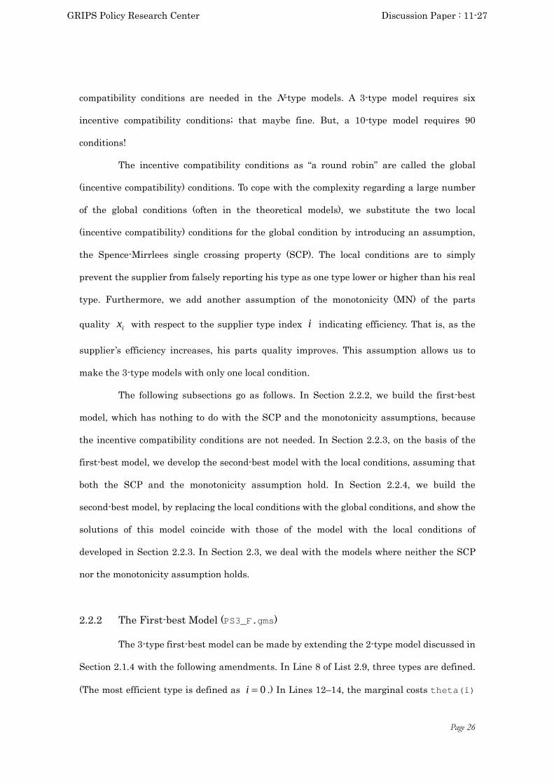
compatibility conditions are needed in the N-type models. A 3-type model requires six
incentive compatibility conditions; that maybe fine. But, a 10-type model requires 90
conditions!
The incentive compatibility conditions as “a round robin” are called the global
(incentive compatibility) conditions. To cope with the complexity regarding a large number
of the global conditions (often in the theoretical models), we substitute the two local
(incentive compatibility) conditions for the global condition by introducing an assumption,
the Spence-Mirrlees single crossing property (SCP). The local conditions are to simply
prevent the supplier from falsely reporting his type as one type lower or higher than his real
type. Furthermore, we add another assumption of the monotonicity (MN) of the parts
quality ix with respect to the supplier type index i indicating efficiency. That is, as the
supplier’s efficiency increases, his parts quality improves. This assumption allows us to
make the 3-type models with only one local condition.
The following subsections go as follows. In Section 2.2.2, we build the first-best
model, which has nothing to do with the SCP and the monotonicity assumptions, because
the incentive compatibility conditions are not needed. In Section 2.2.3, on the basis of the
first-best model, we develop the second-best model with the local conditions, assuming that
both the SCP and the monotonicity assumption hold. In Section 2.2.4, we build the
second-best model, by replacing the local conditions with the global conditions, and show the
solutions of this model coincide with those of the model with the local conditions of
developed in Section 2.2.3. In Section 2.3, we deal with the models where neither the SCP
nor the monotonicity assumption holds.
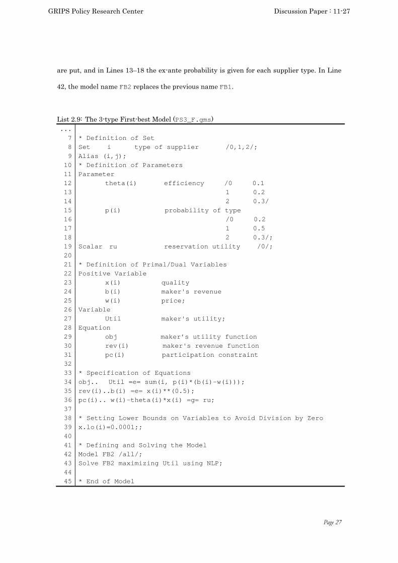
2.2.2 The First-best Model (PS3_F.gms)
The 3-type first-best model can be made by extending the 2-type model discussed in
Section 2.1.4 with the following amendments. In Line 8 of List 2.9, three types are defined.
(The most efficient type is defined as 0i .) In Lines 12–14, the marginal costs theta(i)
GRIPS Policy Research Center Discussion Paper : 11-27
Page 27
are put, and in Lines 13–18 the ex-ante probability is given for each supplier type. In Line
42, the model name FB2 replaces the previous name FB1.
List 2.9: The 3-type First-best Model (PS3_F.gms) ...
7 * Definition of Set 8 Set i type of supplier /0,1,2/; 9 Alias (i,j); 10 * Definition of Parameters 11 Parameter 12 theta(i) efficiency /0 0.1 13 1 0.2 14 2 0.3/ 15 p(i) probability of type 16 /0 0.2 17 1 0.5 18 2 0.3/; 19 Scalar ru reservation utility /0/; 20 21 * Definition of Primal/Dual Variables 22 Positive Variable 23 x(i) quality 24 b(i) maker's revenue 25 w(i) price; 26 Variable 27 Util maker's utility; 28 Equation 29 obj maker’s utility function 30 rev(i) maker's revenue function 31 pc(i) participation constraint 32 33 * Specification of Equations 34 obj.. Util =e= sum(i, p(i)*(b(i)-w(i))); 35 rev(i)..b(i) =e= x(i)**(0.5); 36 pc(i).. w(i)-theta(i)*x(i) =g= ru; 37 38 * Setting Lower Bounds on Variables to Avoid Division by Zero 39 x.lo(i)=0.0001;; 40 41 * Defining and Solving the Model 42 Model FB2 /all/; 43 Solve FB2 maximizing Util using NLP; 44 45 * End of Model
GRIPS Policy Research Center Discussion Paper : 11-27

Page 28
2.2.3 The Second-best Model with the Local Incentive Compatibility Conditions
(PS3_S.gms)
The second-best model must have the incentive compatibility condition, which is
the only difference from the first-best model. As stated before, the complexity of the
second-best model is centered on the incentive compatibility condition.
Before moving into the second-best model, we explain the relationships between
the global and local incentive conditions in a matrix format (Table 2.5). In that table all the
types that the i -th type supplier can report truly and falsely are shown as dark and light
grey areas.
Table 2.5: Global and Local Incentive Compatibility Conditions Reported Supplier Type
0 … 1i i 1i … 1N
Tru
e S
upp
lier
Typ
e
0 00 |U … 01 | iU 0|iU 01 | iU … 01 | NU… …
1i 1| iiU
i iU |0 … iiU |1 iiU | iiU |1… iNU |1
1i 1| iiU
… … 1N 1| NiU
For the sake of the explanation below, we define the i -th supplier’s utility
generated when he reports his type as the j -th supplier as ijU | . The global incentive
compatibility conditions to discourage him from false reporting can be written as follows:
ijii UU || j
This is equivalent to:
iii UU || 0
iii UU || 1
iii UU || 2
GRIPS Policy Research Center Discussion Paper : 11-27

Page 29
…
iiii UU || 1
iiii UU || (Note that this is a trivial one.)
iiii UU || 1
…
iNii UU || 1
One can see that the number of the global conditions increases rapidly, as the
number of types increases. There are two methods to cope with this difficulty. The first
method is to introduce the SCP assumption and to substitute the local conditions for the
global ones. If the SCP assumption holds, only two conditions are needed for each supplier
among these many. The one condition, denoted as LICD, is to discourage a supplier from
reporting his type as one type lower than his real type. The other condition, denoted as
LICU, is to discourage him from reporting one type higher:
iiii UU || 1 i (LICU)
iiii UU || 1 i (LICD)
These conditions are imposed for the cases shown in the dark grey areas in Table 2.5.
The second method to cope with the difficulty is to add the condition of the
monotonicity (MN) regarding the parts quality ix as:
Nxx ...0
If the monotonicity condition is added, either LICD or LICU is sufficient for the local
conditions.
The commonly used approach to the second method is to build and solve the model
without imposing MN, and ascertain that the solutions do satisfy MN. If the solutions
satisfy MN, the omission of MN in the model is justified. Conversely, if MN is not satisfied in
the solutions, one must rewrite the model in such a way as to add either MN or LICD (or
GRIPS Policy Research Center Discussion Paper : 11-27

Page 30
LICU) explicitly. (More detailed explanation will be given in Section 2.3.3.) We follow this
approach here.
In our assumed supplier’s utility iiii xuwU , and iiii xxu , , the first
derivative of u with respect to ix , i.e., xu is a decreasing function with respect to i ;
therefore, the SCP is satisfied. Accordingly, we can simplify the model by replacing the
global conditions with the local conditions.
In the following, we develop the model with LICD but without MN as:.
i
iii wxbpUtilmax (2.1’)
subject to
5.0ii xxb i (2.2)
ruxw iii i (2.3’)
11 iiiiii xwxw i (2.5)
In the model (PS3_S.gms), LICD (2.5) appears in Line 38. The supplier who is by one type
less efficient than the i -th type supplier can be written as 1i , as intuition tells you.
The participation constraint is set for all the suppliers as in the first-best model to
compute the information rent earned by each supplier, which is indicated as the solved
slacks of the constraints (Line 37 of List 2.10). As this constraint is not binding for other
than the supplier 2i (i.e., the most inefficient supplier), none of these extra constraints
does not distort the solutions at all.
List 2.10: The 3-type Second-best Model (PS3_S.gms) ...
7 * Definition of Set 8 Set i type of supplier /0,1,2/; 9 Alias (i,j); 10 * Definition of Parameters 11 Parameter 12 Theta(i) efficiency /0 0.1
GRIPS Policy Research Center Discussion Paper : 11-27

Page 31
13 1 0.2 14 2 0.3/ 15 p(i) probability of type 16 /0 0.2 17 1 0.5 18 2 0.3/; 19 Scalar ru reservation utility /0/; 20 21 * Definition of Primal/Dual Variables 22 Positive Variable 23 x(i) quality 24 b(i) maker's revenue 25 w(i) price; 26 Variable 27 Util maker's utility; 28 Equation 29 obj maker’s utility function 30 rev(i) maker's revenue function 31 pc(i) participation constraint 32 licd(i) incentive compatibility constraint; 33 34 * Specification of Equations 35 obj.. Util =e= sum(i, p(i)*(b(i)-w(i))); 36 rev(i)..b(i) =e= x(i)**(0.5); 37 pc(i).. w(i)-theta(i)*x(i) =g= ru; 38 licd(i)..w(i)-theta(i)*x(i) =g= w(i+1)-theta(i)*x(i+1); 39 40 * Setting Lower Bounds on Variables to Avoid Division by Zero 41 x.lo(i)=0.0001;; 42 43 * Defining and Solving the Model 44 Model SB3 /all/; 45 Solve SB3 maximizing Util using NLP; 46 47 * End of Model
The solution of the model is shown in its output file shown in List 2.11.
List 2.11: Output File of the 3-type Second-best Model (PS3_S.lst) ... 125 ---- EQU rev maker's revenue function 126 127 LOWER LEVEL UPPER MARGINAL 128 129 0 . . . 0.200
GRIPS Policy Research Center Discussion Paper : 11-27

Page 32
130 1 . . . 0.500 131 2 . . . 0.300 132 133 ---- EQU pc participation constraint 134 135 LOWER LEVEL UPPER MARGINAL 136 137 0 . 0.522 +INF . 138 1 . 0.088 +INF . 139 2 . . +INF -1.000 140 141 ---- EQU licd incentive compatibility constraint 142 143 LOWER LEVEL UPPER MARGINAL 144 145 0 . . +INF -0.200 146 1 . . +INF -0.700 147 2 . . +INF . 148 149 ---- VAR x quality 150 151 LOWER LEVEL UPPER MARGINAL 152 153 0 1.0000E-7 25.000 +INF 5.7724E-8 154 1 1.0000E-7 4.340 +INF EPS 155 2 1.0000E-7 0.879 +INF EPS 156 157 ---- VAR b maker's revenue 158 159 LOWER LEVEL UPPER MARGINAL 160 161 0 . 5.000 +INF . 162 1 . 2.083 +INF . 163 2 . 0.937 +INF . 164 165 ---- VAR w price 166 167 LOWER LEVEL UPPER MARGINAL 168 169 0 . 3.022 +INF . 170 1 . 0.956 +INF . 171 2 . 0.264 +INF . 172 173 LOWER LEVEL UPPER MARGINAL 174 175 ---- VAR Util -INF 1.161 +INF . ...
GRIPS Policy Research Center Discussion Paper : 11-27

Page 33
2.2.4 Comparison of the First-best and the Second-best Solutions
The comparison of the first-best (PS3_F.lst) and second-best solutions
(PS3_S.lst) is shown in Table 2.6.
Table 2.6: Solutions of the 3-type First-best and Second-best Models
Variable Variable
Name in the Program
Supplier Type
Second-best Solution
First-best Solution Gap
Parts Quality x(i) 0 25.00 25.00 0.00 1 4.34 6.25 –1.91 2 0.88 2.78 –1.90
Maker’s Revenue
b(i) 0 5.00 5.00 –0.00 1 2.08 2.50 –0.42 2 0.94 1.67 –0.73
Price w(i) 0 3.02 2.50 0.52
1 0.96 1.25 –0.29 2 0.26 0.83 –0.57
Maker’s Utility Util 1.16 1.37 –0.21 Supplier’s Utility (=Info. Rent)
pc.l(i) -pc.lo(i)
0 0.52 0.00 0.52 1 0.09 0.00 0.09
2 0.00 0.00 0.00 Lag. Mult. of Incentive Comp. Const.
licd.m(i) 0 –0.20 – – 1 –0.70 – – 2 0.00 – –
Lag. Mult. of Participation Constraint
pc.m(i) 0 0.00 0.00 – 1 0.00 0.00 – 2 –1.00 –1.00 –
Compared with the first-best solutions, the parts quality x(i) in the second-best
solutions is the same only for the most efficient supplier; the quality is lower for all the other
suppliers. This corresponds to the fact that the price w(i) net of the information rent
remains the same for the most efficient supplier increases, while that of all the others
decreases.
In order to prevent the (not-the-least efficient) suppliers from reporting the less
efficient suppliers’ types, the maker must make a liberal offer to these suppliers in the
GRIPS Policy Research Center Discussion Paper : 11-27

Page 34
second-best case than the one in the first-best case. The maker need not be too liberal; this
liberality is determined at such a level that these suppliers can receive no extra gain even
though they report their types falsely. The incentive compatibility conditions are binding
only for 0i and 1i . Those conditions are not binding for the least efficient supplier
2i , because he has no less-efficient supplier to pretend for an extra gain. Therefore, his
participation constraint is binding; he can obtain just as much as his reservation utility
level.
The information rents gained by the more efficient suppliers ( 0i and 1i ) are
shown as the slacks in their respective participation constrains (Lines 137 and 138 of List
2.11). As the reservation utility is set at zero, their rents immediately indicate their utility
levels. The price of the intermediately efficient supplier ( 1i ) becomes lower than that in
the first-best case, but he obtains strictly positive utility generated by his information rents
offsetting the losses from the lower price. Needless to say, the utility of the most efficient
supplier ( 0i ) increases.
The maker’s utility decreases for two reasons. The first is the loss resulted from the
degraded parts quality supplied by those but the most efficient one. The second is the
information rents exploited by those but the least efficient one.
The solutions show the monotonicity of the parts quality ix . In other words, the
more efficient the supplier is, the higher his parts quality is. Thus, the omission of MN in
the models can be justified.
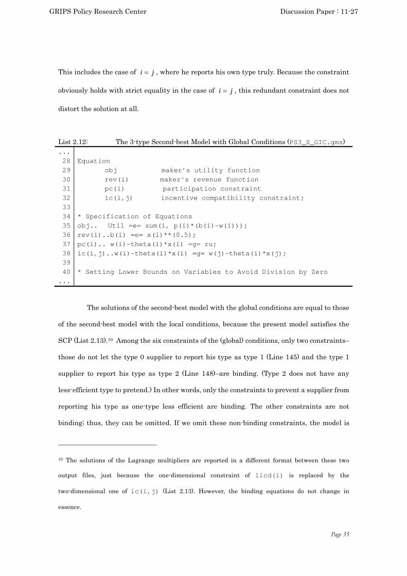
2.2.5 The Second-best Model with the Global Conditions (PS3_S_GIC.gms)
In this subsection, we develop the second-best model by replacing the local
conditions in the previous model with the global conditions, and analyze the solutions. Line
38 of List 2.12 shows the conditions of (2.4). Note that the constraint ic carries two suffixes:
i and j, and “,” is inserted between i and j. The incentive compatibility constraint
ic(i,j) prevents the i -th type supplier from gaining extra by reporting his type as “j”.
GRIPS Policy Research Center Discussion Paper : 11-27
Page 35
This includes the case of ji , where he reports his own type truly. Because the constraint
obviously holds with strict equality in the case of ji , this redundant constraint does not
distort the solution at all.
List 2.12: The 3-type Second-best Model with Global Conditions (PS3_S_GIC.gms) ... 28 Equation 29 obj maker’s utility function 30 rev(i) maker's revenue function 31 pc(i) participation constraint 32 ic(i,j) incentive compatibility constraint; 33 34 * Specification of Equations 35 obj.. Util =e= sum(i, p(i)*(b(i)-w(i))); 36 rev(i)..b(i) =e= x(i)**(0.5); 37 pc(i).. w(i)-theta(i)*x(i) =g= ru; 38 ic(i,j)..w(i)-theta(i)*x(i) =g= w(j)-theta(i)*x(j); 39 40 * Setting Lower Bounds on Variables to Avoid Division by Zero
...
The solutions of the second-best model with the global conditions are equal to those
of the second-best model with the local conditions, because the present model satisfies the
SCP (List 2.13).10 Among the six constraints of the (global) conditions, only two constraints–
those do not let the type 0 supplier to report his type as type 1 (Line 145) and the type 1
supplier to report his type as type 2 (Line 148)–are binding. (Type 2 does not have any
less-efficient type to pretend.) In other words, only the constraints to prevent a supplier from
reporting his type as one-type less efficient are binding. The other constraints are not
binding; thus, they can be omitted. If we omit these non-binding constraints, the model is
10 The solutions of the Lagrange multipliers are reported in a different format between these two
output files, just because the one-dimensional constraint of licd(i) is replaced by the
two-dimensional one of ic(i,j) (List 2.13). However, the binding equations do not change in
essence.
GRIPS Policy Research Center Discussion Paper : 11-27

Page 36
boiled down into the model with the local conditions of LICD (2.5). Therefore, the solutions
of the two models are naturally identical (Lists 2.10 and 2.11).
List 2.13: Output File of the 3-type Second-best Model with the Global Condition (PS3_S_GIC.lst)
... 133 ---- EQU pc participation constraint 134 135 LOWER LEVEL UPPER MARGINAL 136 137 0 . 0.522 +INF . 138 1 . 0.088 +INF . 139 2 . . +INF -1.000 140
141 ---- EQU ic incentive compatibility constraint
142
143 LOWER LEVEL UPPER MARGINAL
144
145 0.1 . . +INF -0.200
146 0.2 . 0.346 +INF .
147 1.0 . 2.066 +INF EPS
148 1.2 . . +INF -0.700
149 2.0 . 4.478 +INF .
150 2.1 . 0.346 +INF .
...
2.3 The Extensions of the Models
In this section, the models developed so far will be extended in the following two
directions. The first one is to increase the number of supplier types. In Section 2.3.1, we
present the model with 10 types. The second one is to develop models without the
simplifying assumptions, such as the SCP and MN. In Section 2.3.2, we develop the model
where the SCP does not hold. In Section 2.3.3, we deal with the model where the sufficient
condition of monotonicity does not hold, while the SCP is satisfied.
2.3.1 The Models with a Large number of Supplier Types (PS10_S.gms)
When the number of types increases, the theoretical models become difficult in
conducting analyses. However, only minimal adjustments are required for our numerical
GRIPS Policy Research Center Discussion Paper : 11-27

Page 37
models with a large number of supplier types. For example, to prepare a 10-type model
( 9...,,2,1,0i ), it is sufficient to rewrite the Set statement for the supplier types as follows
(List 2.14):
Set i type of supplier /0*9/;
The symbol “*” (asterisk) simplifies the expression of the indices as consecutive
numbers. The program stated above equivalently can be written as follows:
Set i type of supplier /0,1,2,3,4,5,6,7,8,9/;
List 2.14: The 10-type Model (PS10_S.gms) ...
7 * Definition of Set
8 Set i type of supplier /0*9/;
9 Alias (i,j);
10 * Definition of Parameters
11 Parameter
12 theta(i) efficiency
13 p(i) probability of type;
14 theta(i)=ord(i)/card(i);
15 p(i)=1/card(i);
...
(In a 100-type model, it is sufficient to replace “9” by “99” though the trial version of GAMS,
however, cannot solve the 100-type model because of the model size limitation.) Lines 14–15
of List 2.14 compute the value of efficiency parameter i with the same intervals for all i ’s
and the ex-ante probability ip over all i ’s with random draws from a uniform distribution.
Instead, specific numbers can be given, if one wishes.
2.3.2 The Second-best Models where the SCP does not Hold (PS3_SCP.gms)
When the SCP does not hold, we must use the global conditions, instead of the local
GRIPS Policy Research Center Discussion Paper : 11-27

Page 38
conditions. The structure of the model is the same as the model with the global conditions
shown in Section 2.2.5. As an example, let us consider the i -th type supplier’s utility
function: iiiiii xxu 21, ,where 10 ix , 10 i , in place of the
original one: iiii xxu , . With this alternative u function, the value of its cross
partial derivative with respect to ix and i (i.e., ixu 21 ) is positive if 5.0i
but negative if 5.0i . Thus, this u does not satisfy the SCP assumption.
The maker’s utility maximization problem is as follows:
i
iii wxbpUtilmax (2.1’)
subject to
5.0ii xxb i (2.2)
ruxw iiiii 21 i (2.3’’)
jiiijiiiii xwxw 22 11 ji (2.4’)
In List 2.15, the participation constraints (2.3”) is declared as pc(i), and the
global conditions as ic(i,j). The function sqr(…) means square. Line 52 defines the
second-best model with the global conditions as SB_gic_wo_SCP.
Just for the sake of comparison, in the same program, we use the local conditions
(LICD, LICU) although the model must be solved with the global conditions for the correct
solution. In Lines 43–46, these local conditions are shown as licd(i) and licu(i). In Line
53, the model with the local conditions is defined as SB_lic_wo_SCP.
List 2.15: The Second-best Model that Does not Satisfy the SCP (PS3_S_SCP.gms) ... 10 * Definition of Parameters 11 Parameter 12 theta(i) efficiency /0 0.1 13 1 0.4
GRIPS Policy Research Center Discussion Paper : 11-27

Page 39
14 2 0.9/ 15 p(i) probability of type 16 /0 0.2 17 1 0.5 18 2 0.3/;
... 28 Equation
... 32 ic(i,j) incentive compatibility constraint 33 licd(i) incentive compatibility constraint 34 licu(i) incentive compatibility constraint; 35 36 * Specification of Equations 37 obj.. Util =e= sum(i, p(i)*(b(i)-w(i))); 38 rev(i)..b(i) =e= x(i)**(0.5); 39 pc(i).. w(i) -(theta(i)+(1-theta(i)+sqr(theta(i)))*x(i)) 40 =g= ru; 41 ic(i,j)..w(i) -(theta(i)+(1-theta(i)+sqr(theta(i)))*x(i)) 42 =g= w(j) -(theta(i)+(1-theta(i)+sqr(theta(i)))*x(j)); 43 licd(i)..w(i) -(theta(i)+(1-theta(i)+sqr(theta(i)))*x(i)) 44 =g= w(i+1)-(theta(i)+(1-theta(i)+sqr(theta(i)))*x(i+1)); 45 licu(i)..w(i) -(theta(i)+(1-theta(i)+sqr(theta(i)))*x(i)) 46 =g= w(i-1)-(theta(i)+(1-theta(i)+sqr(theta(i)))*x(i-1)); 47 48 * Setting Lower Bounds on Variables to Avoid Division by Zero 49 x.lo(i)=0.0001; 50 51 * Defining and Solving the Model 52 Model SB_gic_wo_SCP /obj, rev, pc, ic/; 53 Model SB_lic_wo_SCP /obj, rev, pc, licd, licu/; 54 55 Solve SB_gic_wo_SCP maximizing Util using NLP; 56 Solve SB_lic_wo_SCP maximizing Util using NLP; 57 * End of Model
In the second-best model with the global conditions, the solutions of the parts
quality do not satisfy the monotonicity (Table 2.7). However, because the local conditions are
not used, the monotonicity is not required; thus, the solutions are correct.
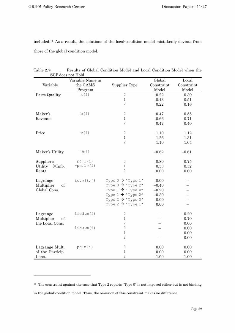
The Lagrange multipliers of three cases (Type 0 reports “Type 2”, Type 1 does “Type
0”, and Type 1 does “Type 2”) are non-zero in the global-condition model; thus, the conditions
for these three cases cannot be omitted. However, in the local-condition model, among these
three global conditions, the condition to prevent Type 0 from reporting “Type 2” is not
GRIPS Policy Research Center Discussion Paper : 11-27
Page 40
included.11 As a result, the solutions of the local-condition model mistakenly deviate from
those of the global-condition model.
Table 2.7: Results of Global Condition Model and Local Condition Model when the SCP does not Hold
Variable Variable Name in
the GAMS Program
Supplier Type Global
Constraint Model
Local Constraint
Model Parts Quality x(i) 0 0.22 0.30 1 0.43 0.51 2 0.22 0.16 Maker’s Revenue
b(i) 0 0.47 0.55 1 0.66 0.71 2 0.47 0.40
Price
w(i) 0 1.10 1.12 1 1.26 1.31 2 1.10 1.04
Maker’s Utility Util –0.62 –0.61 Supplier’s Utility (=Info. Rent)
pc.l(i) -pc.lo(i)
0 0.80 0.75 1 0.53 0.52 2 0.00 0.00
Lagrange Multiplier of Global Cons.
ic.m(i,j) Type 0 ”Type 1” 0.00 – Type 0 ”Type 2” –0.40 – Type 1 ”Type 0” –0.20 – Type 1 ”Type 2” –0.30 – Type 2 ”Type 0” 0.00 – Type 2 ”Type 1” 0.00 –
Lagrange Multiplier of the Local Cons.
licd.m(i) 0 – –0.20 1 – –0.70 2 – 0.00
licu.m(i) 0 – 0.00 1 – 0.00 2 – 0.00
Lagrange Mult. of the Particip. Cons.
pc.m(i) 0 0.00 0.00 1 0.00 0.00 2 –1.00 –1.00
11 The constraint against the case that Type 2 reports “Type 0” is not imposed either but is not binding
in the global-condition model. Thus, the omission of this constraint makes no difference.
GRIPS Policy Research Center Discussion Paper : 11-27
Page 41
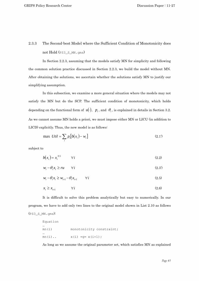
2.3.3 The Second-best Model where the Sufficient Condition of Monotonicity does
not Hold (PS3_S_MN.gms)
In Section 2.2.3, assuming that the models satisfy MN for simplicity and following
the common solution practice discussed in Section 2.2.3, we build the model without MN.
After obtaining the solutions, we ascertain whether the solutions satisfy MN to justify our
simplifying assumption.
In this subsection, we examine a more general situation where the models may not
satisfy the MN but do the SCP. The sufficient condition of monotonicity, which holds
depending on the functional form of u , ip , and i , is explained in details in Section 3.2.
As we cannot assume MN holds a priori, we must impose either MN or LICU (in addition to
LICD) explicitly. Thus, the new model is as follows:
i
iii wxbpUtilmax (2.1’)
subject to
5.0ii xxb i (2.2)
ruxw iii i (2.3’)
11 iiiiii xwxw i (2.5)
1 ii xx i (2.6)
It is difficult to solve this problem analytically but easy to numerically. In our
program, we have to add only two lines to the original model shown in List 2.10 as follows
(PS3_S_MN.gms):
Equation … mn(i) monotonicity constraint; … mn(i).. x(i) =g= x(i+1); As long as we assume the original parameter set, which satisfies MN as explained
GRIPS Policy Research Center Discussion Paper : 11-27

Page 42
in Section 3.1, the solutions of the new model with MN perfectly match those of the original
model without MN. The output file shows (PS3_S_MN.lst) that the newly introduced
constraint mn(i) is not binding.
In contrast, let us consider the following two cases where the parameter sets are
modified regarding with the modified ex-ante probability ip (Case A) and regarding the
modified efficiency i (Case B) so that their solutions do not satisfy MN. We solve these
models with MN (correctly) and without MN (incorrectly) (Table 2.8).
Table 2.8: Solutions of Models that do not Satisfy Monotonicity Case A Case B
w/ MN w/o MN w/ MN w/o MN
0x 25.000 25.000 25.000 25.000
1x 1.680 1.000 1.902 1.731
2x 1.680 1.860 1.902 2.250
In these numerical examples, we can obtain the correct solutions only when MN (or
LICU) is imposed. The correct solutions show step-wise monotonicity of the parts quality ix .
(We can verify that these solutions are correct, by comparing them with those computed by
the global-condition models.) Note, however, that we are discussing the sufficient condition;
thus, we may obtain the correct solutions even if neither MN nor LICU is imposed. This is to
be discussed in the next section.
3. The Monotonicity Conditions
In Section 2, we build the model where the sufficient condition of monotonicity of
the parts quality holds and the one where it does not hold, and discuss the differences in
their solutions. The natural question would be twofold. The first is to what extent the
GRIPS Policy Research Center Discussion Paper : 11-27
Page 43
sufficient condition of monotonicity holds. The second is how much likely we can get correct
solutions even without imposing MN. In this section, by fully exploiting the advantages of
the numerical approach in combination with a Mote Carlo simulation method, we try to
obtain some idea about these questions.
We first formulate of the sufficient condition in our model framework. Then, we
directly focus on the question stated above by computing two kinds of probabilities. That is,
we derive (A) the probability that the sufficient condition of the monotonicity holds and (B)
the probability that monotonicity occurs, whether the sufficient condition holds or not.
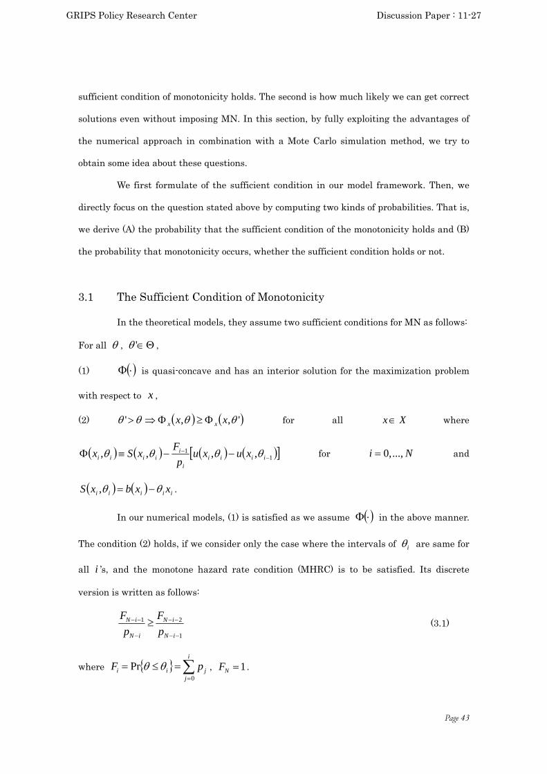
3.1 The Sufficient Condition of Monotonicity
In the theoretical models, they assume two sufficient conditions for MN as follows:
For all , ' ,
(1) is quasi-concave and has an interior solution for the maximization problem
with respect to x ,
(2) ',,' xx xx for all Xx where
11 ,,,, iiiii
iiiii xuxu
p
FxSx for Ni ...,,0 and
iiiii xxbxS , .
In our numerical models, (1) is satisfied as we assume in the above manner.
The condition (2) holds, if we consider only the case where the intervals of i are same for
all i ’s, and the monotone hazard rate condition (MHRC) is to be satisfied. Its discrete
version is written as follows:
1
21
iN
iN
iN
iN
p
F
p
F (3.1)
where
i
jjii pF
0
Pr , 1NF .
GRIPS Policy Research Center Discussion Paper : 11-27
Page 44
3.2 The Probability that Monotonicity Holds (PS3_S_MN.gms)
To estimate the probability (A) that monotonicity holds, we prepare a model
distinguishing 10 types of suppliers assuming (1) i whose intervals are the same for all
i ’s and (2) the ex-ante probability ip over all i ’s generated with random draws from a
uniform distribution.
In the first stage to estimate the probability that the sufficient condition of
monotonicity, i.e., MHRC (3.1), holds, we simulate 1,000 Monte Carlo draws. This result
implies the degree of its restrictiveness.
In the second stage, we make two models (SB_lic and SB_lic2); the one without
the monotonicity constraint mn(i) and the one with its constraint. While the latter model
always yields correct solutions, the former one may do so because the omitted condition
MHRC (3.1) is just a sufficient condition–not the necessary one. If both models generate the
identical solutions, it means that monotonicity holds, whether the sufficient condition of
monotonicity hold. The probability (B) that such cases occur is the one that we pursue to
obtain in the second stage. The input file of the second stage looks complicated partly
because its randomly computes the ex-ante probability p(i) and partly because the
program includes two models with and without MN (SB_LIC and SB_LIC2).
The results are as follows. In the first stage, MHRC (3.1) holds in only one case
among the randomly generated 1,000 cases. (In other words, the probability (A) that the
sufficient condition of monotonicity holds is 0.1%.) In the second stage, with the same
random parameter sets of ip for 1,000 cases, the two models with and without MN yield
the identical solutions only in seven cases. (In other words, the probability (B) that
monotonicity holds–whether its sufficient condition holds or not–is 0.7%.
It should be noted that the probabilities mentioned above may differ depending on
many parameters. When we consider more supplier types, we find their likelihood decreases
GRIPS Policy Research Center Discussion Paper : 11-27

Page 45
because MHRC (3.2) is a joint condition for all the chains between adjacent supplier types.
For example, if we consider only five supplier types (PS5_S_MN.gms), the probability of (A)
is 24% and (B) is 36%. Although we need some reservations in generalizing the results of our
numerical experiments, the MHRC would be a more restrictive condition than usually
expected.
4. Concluding Remarks
In this paper, we build and solve the numerical 2-type and 3-type models of the
parts supply problems. Although their solutions depend on our assumed functional forms
and parameters, we obtain the reasonable solutions as their theories predict. For example,
in the second-best model, only the most efficient supplier maintains the first-best level parts
quality. Since that the suppliers except for the least efficient one can report his type falsely
under asymmetric information, they can obtain extra gains as information rents. In contrast,
the least efficient supplier can obtain no extra gain. In total, the maker’s utility level
decreases from her first-best level.
We formulate the parts supply problems as non-linear programming problems.
Then, by specifying their functional forms and feeding illustrative values into parameters,
we build and solve them numerically. Taking advantage of this numerical approach, this
paper demonstrates the usefulness of this approach for the contract theory analysis in
various ways. First, the information rent, which is the most crucial variable in the
asymmetric information problems, can be directly computed as the solutions of the Lagrange
multipliers for the incentive compatibility constraints as shown in the EQU block of the
GAMS output file. Second, when the number of supplier types increases, the theoretical
models need additional assumptions such as the SCP and monotonicity to simplify their
analyses. As a result their analyses are confined to the cases that those assumptions hold. In
contrast, numerical models can deal with the cases whether those simplifying assumptions
hold or not. Third, we apply the Monte-Carlo simulation method so that we can infer how
GRIPS Policy Research Center Discussion Paper : 11-27

Page 46
restrictive the assumption of monotonicity is.
At the same time, we must recognize the limitations of our numerical approach.
Just as the application of the theoretical models is narrowed by those simplifying
assumptions, our numerical approach depends on our assumed functional forms and
parameter sets. We should not hastily claim any general conclusion from numerical model
solutions. It would be useful to take both the theoretical approach and the numerical one
complementarily. We had better go back and forth between the theoretical models and the
numerical models.
At the end, all the models developed in this paper are listed in Table 2.9.
Table 2.9: Models for the Parts Supply Problem
Input File Name No. of Types
Asymmetric Information
Incentive Compatibility
Constraint
Monotonicity Constraint Note
PS2_F_eff.gms 2 No – – Only for efficient suppliers
PS2_F_inf.gms 2 No – – Only for inefficient suppliers
PS2_F.gms 2 No – – PS2_S.gms 2 Yes Local No PS2_F&S.gms 2 No/Yes Local No PS3_F.gms 3 No – – PS3_S.gms 3 Yes Local No PS3_S_GIC.gms 3 Yes Global – PS3_S_SCP.gms 3 Yes Global/Local – The solution of
the local constraint model is incorrect.
PS3_S_MN.gms 3 Yes Local Yes PS5_S_MN.gms 5 Yes Local/Global Yes/
No The solution of the model without MN is incorrect.
PS10_S.gms 10 Yes Local No PS10_S_MN.gms 10 Yes Local/Global Yes/
No The solution of the model without MN is incorrect.
GRIPS Policy Research Center Discussion Paper : 11-27

Page 47
Acknowledgement
This paper includes the research results by Hashimoto as visiting researcher at the
National Graduate Institute for Policy Studies. He expresses thanks to research supports
offered by the National Graduate Institute for Policy Studies.
References
Brooke, A., Kendrick, D., Meeraus, A., Raman, R., Rosenthal, R. E. (2010), GAMS A User’s
Guide, GAMS Development Corporation, Washington, D.C.
Hashimoto, H., Hamada K., Hosoe N. (2011), "Keiyakuriron: Puroguramingu Moderu
Apurochi [Contract Theory: A Programming-Model Approach]," GRIPS Discussion
Paper 10-34 (in Japanese).
Hosoe, N., Gasawa, K., Hashimoto, H. (2010), Textbook of Computable General Equlibrium
Modelling, Programming and Simulations, Palgrave Macmillan.
Itoh, H. (2003), Keiyaku no Keizai Riron (A Course in Contract Theory), Yuhikaku (in
Japanese).
McCarl, B. A. (2009), Expanded GAMS User Guide, version 23.3.
Varian, H. (1992), Macroeconomic Analysis, 3rd Ed., Norton.
GRIPS Policy Research Center Discussion Paper : 11-27